Diversi…cation and Performance:

Linking Relatedness, Market Structure and the Decision to Diversify

Ron Adner and Peter Zemsky¤

January 15, 2012

Abstract

An extensive empirical literature in strategy and …nance studies the performance im-

plications of corporate diversi…cation. Two core debates in the literature concern the

existence of a diversi…cation discount and the relative importance of industry relatedness

and market structure for the performance of diversi…ers. We address these debates by

building a formal model in which the extent of diversi…cation is endogenous and depends

on the degree of industry relatedness. Firms’ diversi…cation choices a¤ect both their own

competitiveness and market structure. We …nd a non-monotonic e¤ect of relatedness on

performance: while greater relatedness increases the competitiveness of diversi…ed …rms,

it can also spur additional diversi…cation, thereby eroding market structure and perfor-

mance. In addition, our model elucidates the emergence of heterogeneity in …rm scope

strategies. We use the model to generate data and show how the negative e¤ect of relat-

edness on market structure can give rise to spurious inference of a diversi…cation discount

in cross-sectional regressions.

Key words: diversi…cation discount, horizontal scope of the …rm, formal foundations of

strategy

¤We would like to thank Pierre Dussauge, Javier Gimeno, Bruce Kogut, Glenn McDonald, Anita McGa-han, Mary O’Sullivan, Dimo Ringov, Belen Villalonga and seminar participants at the Atlanta CompetitiveAdvantage Conference for their helpful comments.

1. Introduction

A fundamental question in corporate strategy is the choice of horizontal scope – the set of

industries and market segments in which a …rm competes. Governing this choice is a trade-o¤

between the threat of losing focus and the opportunity to grow and exploit synergies. This

trade-o¤ raises the question of whether and when diversi…cation is pro…table. Understanding

the drivers of successful diversi…cation has been a pillar of the strategy research agenda from

the founding of the …eld (e.g. Penrose, 1959; Anso¤, 1957).

In this paper, we seek to elucidate the relationship between diversi…cation and performance

by developing a formal model in which diversi…cation decisions are endogenous. In so doing,

we contribute to the growing literature on the formal foundations of strategy, which has so

far largely ignored issues of corporate strategy. Prior work on the formal foundations of

strategy has focused on the general issue of value creation and value capture (Brandenberger

and Stuart, 1996; Lippman and Rumelt, 2003; MacDonald and Ryall, 2004), the workings of

strategic factor markets in which …rms acquire valuable resources (Makadok, 2001; Makadok

and Barney, 2001) and on the sustainability of competitive advantage at the business unit level

(Adner and Zemsky, 2006). Given the extensive attention paid to corporate level issues in the

strategy …eld, we think that extending formal work into the realm of corporate strategy is a

natural and important next step.

Empirical work on the relationship between performance and diversi…cation has a long

history in both the strategy literature (e.g., see Ramanujam and Varadarajan, 1989; and

Montgomery, 1994 for reviews) and in the …nance literature (e.g., see Martin and Sayrak,

2003 for a review). Work in …nance, in particular, has centered on a debate between two

competing views of diversi…ed …rms. One view is that diversi…ed …rms are able to exploit

superior information to make better resource allocation choices through their internal capital

markets than could …nancial markets (Caves, 1971; Myers and Majluf, 1984). A competing

view is that diversi…ed …rms are plagued by ine¢ciencies due to agency problems and that

resources would be better allocated between businesses by …nancial markets (Amihud and Lev,

1981; Schliefer and Vishney 1989). The observation that diversi…ed …rms trade at a discount to

their more focused peers is taken as evidence of unresolved agency problems and poor corporate

1

governance. Numerous studies have supported the existence of such a diversi…cation discount

(e.g., Montgomery and Wernerfelt, 1988; Lang and Stulz, 1994; Berger and Ofek, 1995).

The strategy literature, with its fundamental concern with …rm heterogeneity, has had a

di¤erent focus. It has sought to explain di¤erences in performance among diversi…ed …rms.

Early contributions focused on the extent to which relatedness among corporate businesses was

associated with higher returns (Rumelt, 1974; Bettis, 1981). Later contributions sought to link

the nature of …rm resources with the type of diversi…cation in which …rms engaged (Mont-

gomery and Wernerfelt, 1988; Chatterjee and Wernerfelt, 1991). The basic notion, going back

to Penrose (1959), is that the greater the relatedness among the markets within which the

…rm competes, the greater the scope for sharing resources across business units and hence the

greater the performance of diversi…ed …rms. Competing with this internal, resource-based per-

spective on diversi…cation performance, is a research stream that emphasizes the importance

of external competitive pressures, speci…cally the importance of industry attractiveness and

market structure (Christensen and Montgomery, 1981; Montgomery, 1985) and the potential

to manage competition through multi-market contact (Karnani and Wernerfelt, 1985; Gimeno

and Woo, 1999).

In both strategy and …nance, early empirical work took the decision to diversify as exoge-

nous. More recent empirical contributions have explicitly incorporated the endogeneity of the

diversi…cation decision. Several papers use empirical methods (e.g. Heckman, 1979; Deheja

and Wahba, 2001) that control for endogeneity by explicitly allowing for the possibility that

underlying di¤erences among …rms a¤ect both …rm performance and the decision to diversify

(Campa and Kedia, 2002; Villelonga, 2004a, 2004b; Graham et al., 2002). These papers sug-

gest that diversi…ers are di¤erent from non diversi…ers. When researchers control for these

di¤erences, they fail to …nd a diversi…cation discount, and in some cases, they …nd a diversi-

…cation premium. In other words, they argue that weaker …rms are inherently more likely to

diversify, and that it is this underlying weakness that is responsible for their low performance,

rather than their diversi…cation strategy per se. The debate, however, is not yet settled (see

for example the round-table discussion in Villelonga, 2003).

In parallel to these empirical studies, several theoretical papers in …nance have modeled the

diversi…cation decisions of …rms. Borrowing from the strategy literature, these papers usually

2

start with a set of …rms that vary in their capabilities. They then examine the diversi…cation

decisions of individual …rms in isolation from their peers. In Maksimovic and Phillips (2002)

and in Gomes and Livdan (2004) …rms with high productivity specialize in a single industry

while those with lower productivity chose to diversify. In Matsusaka (2001) and in Bernardo

and Chowdhry (2002) …rms choose to engage in costly diversi…cation as a way to search for

new opportunities to leverage their capabilities. Consistent with the recent empirical …ndings,

all of these theories predict a spurious diversi…cation discount. That they obtain these results

with rational, pro…t maximizing …rms calls into question prior claims about the pervasiveness

of agency problems in corporate strategy (Jensen, 1986).

In contrast with the recent …nance literature, which has focused almost exclusively on the

impact of …rm heterogeneity, the strategy literature on diversi…cation has emphasized three

distinct drivers of diversi…cation performance: …rm heterogeneity, industry relatedness and

the extent of competitive pressures. Clearly, each of these drivers of pro…tability should im-

pact the decision to diversify. The received theory, with its exclusive focus on the decision of

isolated …rms, has overlooked the e¤ects of competitive interactions. Recent empirical stud-

ies in strategy (Stern and Henderson, 2004, examining the US personal computer industry;

Bowen and Wiersema, 2005, examining the entry of foreign-based rivals) have begun to explic-

itly link competition and endogenous diversi…cation decisions. We hope that further theory

development can help to guide future empirical work.1

We contribute to the received literature by developing a formal model of diversi…cation

decisions by multiple competing …rms that simultaneously considers industry relatedness and

market structure. The main elements of our model are as follows. There are two industries

and …rms have a choice between a specialist strategy, which involves competing in only one

industry, and a diversi…cation strategy, which involves competing in both industries and in-

curring additional …xed costs. We allow …rms to vary in their competitiveness, either due to

di¤erences in marginal costs or due to di¤erences in consumer willingness to pay for their of-

fer. The degree of industry relatedness determines whether diversi…cation has a positive e¤ect

1 In a recent working paper, Levinthal and Wu (2005) formalize ideas from Penrose (1959) by consideringthe e¤ect of capacity constrained capabilities on diversi…caiton decisions and performance. Their focus oncapabilities and relatedness in a single …rm model complements our focus on competitive interactions andrelatedness in a multi …rm model.

3

on …rm competitiveness (“synergies”) or a negative e¤ect (“loss of focus”). Market structure

depends on the number of rivals in each industry and on their competitiveness.

We decompose the decision to diversify into three elements: the …xed cost associated with

diversi…cation ( ), the revenue growth from entry into the second industry (), and the

e¤ect on revenues in the home industry due to shifts in competitiveness (). A …rm chooses

to diversify when the additional …xed cost burden is less than the net increase in revenue

( +).

A key building block in the analysis is the e¤ect of relatedness on the decision to diver-

sify. Increased relatedness between the industries has two e¤ects. First, increased relatedness

creates more opportunities to share …xed costs across businesses, which lowers the …xed cost

burden associated with diversi…cation. Second, increased relatedness enhances the competi-

tiveness of diversi…ed …rms relative to specialized …rms by creating more opportunities at the

corporate level to reduce marginal costs or increase consumer willingness to pay. Increased

competitiveness increases revenues in both the home market and the target market. Hence,

increased relatedness makes it more likely that diversi…cation is pro…table.

Now consider the impact of increases in relatedness on performance. Holding …xed the

number of diversi…ed and specialized …rms, the pro…ts of diversi…ed …rms increase with re-

latedness. At the same time, the pro…ts of specialized …rms decrease due to the increased

competitiveness of their diversi…ed rivals. However, this does not account for the endogeniety

of diversi…cation decisions. With su¢cient increases in relatedness, …rms that would have

previously chosen to specialize now choose to diversify and enter a second industry. This

deterioration in market structure lowers the pro…ts of both diversi…ers and specialists. Thus,

while the e¤ect of increased relatedness on the pro…ts of specialized …rms is unambiguously

negative, the e¤ect on diversi…ed …rms is non-monotonic. Overall, however, as relatedness

increases from a low level up to a high level we …nd that the pro…ts of all …rms fall.

In many industries one observes di¤erences in …rm scope strategies. For example, au-

tomakers vary in the range of vehicles they produce and the geographies that they serve;

some information technology …rms like IBM and HP pursue broad strategies while other like

SAP and Sun Microsystems pursue more focused strategies. The resource-based view of strat-

egy explains such di¤erences in product market positions with di¤erences in the underlying

4

resource-base of the …rms (Wernerfelt, 1984).

Our theory explains …rm heterogeneity in scope strategy even though all …rms are initially

the same. While one might expect that, absent resource heteroegneity, either all …rms would

chose to diversify or none would, we show that this need not be the case. Rather, we show that

the number of diversi…ed …rms increases incrementally with increases in the degree of market

relatedness. The level of diversi…cation increases incrementally in our model because each new

diversi…er increases competition and this lowers the returns from additional diversi…cation.

Hence, not all …rms will …nd it pro…table to bear the …xed costs of diversifying. The more

related are the two industries, the greater the returns to diversi…cation and the greater the

number of …rms that choose to diversify. Because diversi…cation strategy a¤ects competitive-

ness, the di¤erences in …rm scope strategies give rise to heterogeneity in market shares and

pro…ts.

In our model, diversi…cation can either enhance or reduce the competitiveness of diver-

si…ers relative to specialists. We show that …rms may rationally diversify even in the case

where diversi…cation decreases their competitiveness, thus lowering their revenues in the home

market, because of o¤setting revenue growth in the new market. We consider how outcomes

depend on whether diversi…cation increases or decreases competitiveness. When competitive-

ness decreases, we …nd that either specialists or diversi…ers can have higher pro…ts, depending

on the level of relatedness. We also …nd that …rms face a coordination problem in that there

may be multiple possible levels of diversi…cations. This is because diversi…cation by a given

…rm weakens it in its home market, which can, in turn, induce another …rm to diversify to

exploit this weakness. In contrast, when competitiveness increases with diversi…cation, we …nd

that the pro…ts of diversi…ed …rms are always higher than those of specialists and that there

is a unique level of diversi…cation for a given level of relatedness.

To make explicit the implications of our theory for empirical work on the diversi…cation

discount we use our model to generate cross-sectional data. We analyze the data with di¤erent

OLS regression models. The data are composed of …fty industry pairs that vary in their degree

of relatedness. Within each pair, there are four …rms, which behave according to our theoretical

model. We focus on parameters such that diversi…ers have higher pro…ts than specialists

within any given industry pair. However, industry pairs with more diversi…ed …rms (due to

5

higher levels of relatedness) tend to have lower pro…ts due to increased competitive pressures.

We show that a spurious inference of a diversi…cation discount can arise. This occurs with

empirical speci…cations that do not include e¤ective controls for industry relatedness. We show

that controlling for relatedness will correctly identify the underlying diversi…cation premium,

but that, absent controls for market structure, the regression analysis will lead to incorrect

inference regarding the e¤ect of industry relatedness.

As in any formal modeling exercise, we have had to make important simplifying assump-

tions. These assumption contribute to the model’s tractability and make the mechanisms

underlying the results more transparent. First, we assume that the two industries are sym-

metric in terms of demand and cost conditions. Second, we assume that …rms are initially

homogeneous (but we do show how heterogeneity emerges from …rms’ diversi…cation choices).

Third, we take the number of …rms as exogenous, which means that we can not address issues

of entry and exit or of mergers and acquisitions. However, our model is highly tractable, and

as we discuss in the conclusion, all of these simpli…cations are potential avenues for further

developing a formal theory of corporate strategy.

The paper proceeds as follows. Section 2 describes the model. Section 3 considers the

benchmark where diversi…cation decisions are exogenous. Section 4 characterizes the drivers

of a …rm’s diversi…cation decision and then Section 5 characterizes how the equilibrium level

of diversi…cation varies with market relatedness. Section 6 considers the relative pro…tability

of specialized and diversi…ed …rms. Section 7 presents the analysis of the simulated data and

Section 8 contains a concluding discussion.

2. The Model

We develop a simple, formal model. There are two markets which we label and . These

could be entirely di¤erent industries or they could be two market segments within a single

industry. We assume that the two markets have the same underlying attractiveness including

the same number of potential buyers, . The actual attractiveness and realized size of each

market will, however, vary with the number of …rms that enter. There are 1 …rms that are

initially identical. Firm heterogeneity arises from di¤erences in their choice of scope strategy.

6

STAGE I STAGE II

Choice of Scope Strategy:A-SpecialistB-Specialist

Diversification

Competition among A-Specialists and Diversifiers in Market A

Competition among B-Specialists and Diversifiers in Market B

STAGE I STAGE II

Choice of Scope Strategy:A-SpecialistB-Specialist

Diversification

Competition among A-Specialists and Diversifiers in Market A

Competition among B-Specialists and Diversifiers in Market B

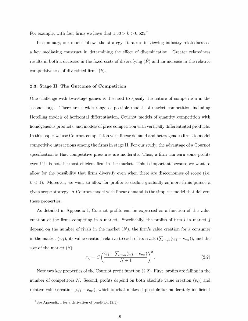
Figure 2.1: The timing of the model

2.1. Model Timing

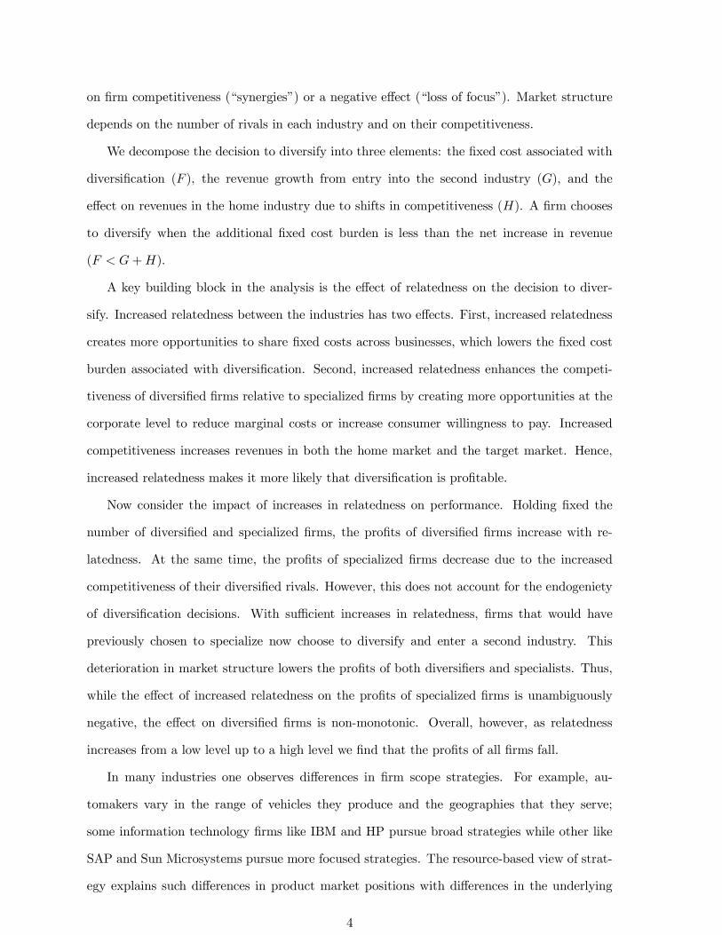
Our model is a two-stage game. In two-stage games, the …rst stage incorporates the decisions

of interest and the second stage incorporates competitive interactions. The timing of the model

is illustrated in Figure 2.1. In the …rst stage, the …rms simultaneously decide on one of three

scope strategies: specialize in market , specialize in market or diversify by entering both

and . Let denote the number of …rms specializing in market , let denote the number

of …rms specializing in market , and let = ¡ ¡ denote the number of …rms that

diversify. In the second stage pro…ts are determined by competition among those …rms active

in each market. Thus, the diversi…ed …rms and the specialized …rms compete in market

; the diversi…ed …rms and the specialized …rms compete in market .

For a two-stage model to be appropriate, it is important that the …rst stage decisions be

harder to change than second stage decisions because …rms are assumed to be committed to

their …rst stage decisions when they compete in the second stage. In our model, diversi…cation

decisions in the …rst stage are stickier and longer term decisions than are price and output

choices in the second stage. Hence, a two-stage model seems appropriate.

We follow the standard approach in studying two-stage games of focusing on subgame

perfect equilibria, which rules out equilibria that can only be supported by non-credible threats.

In addition, we focus on pure strategy equilibria so that …rms are not randomly choosing their

scope strategies.

7

2.2. Stage I: The E¤ects of Diversi…cation

A …rm’s choice of scope in stage I a¤ects both its …xed costs and its competitiveness. The degree

of relatedness between the two markets determines exactly how …xed costs and competitiveness

are impacted by the decision to diversify.

Firms incur a …xed cost of ̂ ¸ 0 when they diversify and enter both markets. ̂ represents

the additional …xed costs required for entry into the second industry, such as new product

design, advertising and qualifying new suppliers. The more related are the two industries –

the more they share technologies and customers – the lower is ̂ .

A …rm’s competitiveness in a market is the level of value that it creates with its product

and service o¤ering. Value creation is the gap between consumers’ willingness to pay for the

…rm’s o¤er and the …rm’s marginal cost of production (Brandenberger and Stuart, 1996). We

let be an index of …rm ’s value creation for a consumer in market . A …rm’s horizontal

scope strategy determines its value creation as follows. Firms specialized in market have

= 0 and = 0 while …rms specialized in market have = 0 and = ,

where is the value creation of specialized …rms in their home market. Diversi…ed …rms have

= = , where is the value creation of diversi…ed …rms.

We make no restriction on the whether or is larger. Let = be the com-

petitiveness of diversi…ed …rms relative to specialized …rms. The case of 1 corresponds

to diseconomies of scope where diversi…ed …rms are less competitive than specialized …rms,

which could result, for example, from a loss of focus. The case of 1 corresponds to syn-

ergies where diversi…ed …rms are more competitive than specialized …rms, which could result,

for example, from the ability to better utilize production capacity or to o¤er customers the

convenience of a “one-stop-shop”. The more related are the two markets in terms of shared

technologies and customers the greater is .

While we make no restriction on whether is greater or less than one, we simplify the

analysis by restricting the range of its possible values to assure that no …rm has such low

competitiveness that it is forced out of a market. Speci…cally we assume that

¡ 1

+ 1

+ 3. (2.1)

8

For example, with four …rms we have that 133 0625.2

In summary, our model follows the strategy literature in viewing industry relatedness as

a key mediating construct in determining the e¤ect of diversi…cation. Greater relatedness

results in both a decrease in the …xed costs of diversifying (̂ ) and an increase in the relative

competitiveness of diversi…ed …rms ().

2.3. Stage II: The Outcome of Competition

One challenge with two-stage games is the need to specify the nature of competition in the

second stage. There are a wide range of possible models of market competition including

Hotelling models of horizontal di¤erentiation, Cournot models of quantity competition with

homogeneous products, and models of price competition with vertically di¤erentiated products.

In this paper we use Cournot competition with linear demand and heterogenous …rms to model

competitive interactions among the …rms in stage II. For our study, the advantage of a Cournot

speci…cation is that competitive pressures are moderate. Thus, a …rm can earn some pro…ts

even if it is not the most e¢cient …rm in the market. This is important because we want to

allow for the possibility that …rms diversify even when there are diseconomies of scope (i.e.

1). Moreover, we want to allow for pro…ts to decline gradually as more …rms pursue a

given scope strategy. A Cournot model with linear demand is the simplest model that delivers

these properties.

As detailed in Appendix I, Cournot pro…ts can be expressed as a function of the value

creation of the …rms competing in a market. Speci…cally, the pro…ts of …rm in market

depend on the number of rivals in the market (), the …rm’s value creation for a consumer

in the market (), its value creation relative to each of its rivals (P

6=( ¡ )), and the

size of the market ():

=

µ +

P6=( ¡ )

+ 1

¶2

. (2.2)

Note two key properties of the Cournot pro…t function (2.2). First, pro…ts are falling in the

number of competitors . Second, pro…ts depend on both absolute value creation () and

relative value creation ( ¡ ), which is what makes it possible for moderately ine¢cient

2See Appendix I for a derivation of condition (2.1).

9

…rms to still produce and earn some pro…ts.

Substituting and into (2.2), the pro…t of a specialized …rm is given by

( ) =

µ + ( ¡ )

+ + 1

¶2

, (2.3)

where is the number of other …rms specializing in the same market and is the number

of diversi…ers. The pro…t of a diversi…ed …rm, which is active in two markets and must incur

the …xed cost ̂ , is

( ) =

µ + ( ¡ )

+

¶2

+

µ + ( ¡ )

+

¶2

¡ ̂ . (2.4)

3. Exogenous Diversi…cation

We start the analysis by considering a baseline case where …rm scope strategies are exogenous.

We take as given the number of …rms , and pursuing each strategy and characterize

the e¤ect of changes in relatedness on the pro…ts of diversi…ed and specialized …rms. The

analysis is straight forward.

Recall that industry relatedness a¤ects both the …xed costs ̂ and competitiveness =

. The pro…ts of specialized …rms are given by (2.3). This is independent of the …xed

costs associated with diversi…cation ̂ . To see the e¤ect of we can rewrite (2.3) as

( ) = 2

µ1 + (1¡ )

+ + 1

¶2

, (3.1)

which is falling in the competitiveness of diversi…ed …rms. As one would expect, the more

competitive are diversi…ed …rms, the lower the pro…ts of specialists.

Now consider the pro…ts of diversi…ed …rms as given by (2.4), which we can rewrite as

( ) = 2

µ + ( ¡ 1)

+ + 1

¶2

+ 2

µ + ( ¡ 1)

+ + 1

¶2

¡ ̂ , (3.2)

which is decreasing in ̂ and increasing in . The greater the additional …xed cost of diversi…-

cation, the lower the pro…ts of diversi…ed …rms; the greater the competitiveness of diversi…ers,

the higher their pro…ts. Thus we have the following:

10

Proposition 3.1. Holding …xed the number of …rms pursuing each strategy: (i) The pro…ts

of diversi…ed …rms are increasing in market relatedness. (ii) The pro…ts of specialized …rms

are decreasing in market relatedness.

As for the relative pro…ts of specialists and diversi…ers, there are too many degrees of

freedom to make any prediction. For ̂ su¢ciently high, , while for ¸ 1 and ̂

su¢ciently low .

A central objective of this paper is to understand how the e¤ect of relatedness on the

absolute and relative performance of specialists and diversi…ers changes when one accounts for

the endogeneity of …rm scope strategies.

4. The Decision to Diversify

A useful …rst step towards endogenizing …rm scope is to examine the incentives for a single

…rm to choose to diversify, holding …xed the scope strategies of the other …rms. Three key

elements that shape a …rm’s decision to diversify, which we label , and .

Consider a situation where there are ¸ 1 …rms specialized in market , one of which is

considering whether or not to diversify. This focal …rm increases its pro…ts by diversifying if

and only if

( ¡ 1 ) ( + 1 ¡ 1 ). (4.1)

We can use (3.1) and (3.2) to rewrite (4.1) as

+

where is the increase in …xed costs required to diversify into market relative to the market

size, is the increase in pro…ts coming from growth in market , and is the change in

pro…ts in the home market . Speci…cally, we have that

=̂

1

2¸ 0

and what matters is the extent of …xed costs ̂ relative to market size, where the relevant

11

measure of market size depends on the number of consumers () and the value created for

consumers ().3

The growth in pro…ts from entry into the target market is

=

µ( + 1)¡ + + 2

¶2

0

which is positive and increasing in the competitiveness of diversi…ers.4 Finally, the e¤ect of

diversi…cation on pro…ts in the home market is

=( ¡ ( ¡ 1))2 ¡ ( + 1¡ )

2

( + + 1)2.

is increasing in and for = 1 we have = 0. Thus for 1 we have that 0 and the

e¤ect on the home market serves to discourage diversi…cation. For 1 we have that 0

and the e¤ect in the home market encourages diversi…cation.

A widely cited managerial prescription for making diversi…cation decisions is to consider

Porter’s three tests (Porter, 1987): the cost-of-entry test, the better-o¤ test and the attractive-

ness test. A bene…t of our formal treatment is that it clari…es some of the ways in which the

factors highlighted in the three tests interact with each other in determining the desirability of

diversi…cation. Our + formula overlaps with Porter’s tests as follows. The quantity

captures the cost of entry, as well as including the impact of market size, which is a key

component of industry attractiveness. The better-o¤ test concerns the e¤ect of diversi…cation

on competitiveness in the target and the existing business, which we capture with . A key

component of the industry attractiveness test is market structure, which in our model is given

by the number of specialized (, ) and diversi…ed () rivals. Our terms and are

determined by the interaction of competitiveness () with market structure (, and ).

While and are exogenous to the model, and depend on , and and hence

on the choices of the other …rms. The next section disentangles this strategic interdependence

and characterizes the equilibrium level of diversi…cation.

3Note that falls with industry relatedness just as ̂ does. Henceforth, we refer to as the …xed costs ofdiversifying, leaving implicit that what matters is …xed costs relative to market size.

4The lower bound on in (2.1) assures that 0.

12

5. The Level of Diversi…cation

We now characterize the equilibrium level of diversi…cation and how it varies with the extent

of market relatedness. We also consider whether there is a unique equilibrium level of diversi…-

cation or whether strategic interdependencies create multiple possible levels of diversi…cation.

Why is multiplicity more than a technical matter? Consider how the sentiment towards diver-

si…cation has varied over time, from the 1960s, when diversi…cation was regarded with favor, to

the 1980s, when it was regarded with suspicion (Schliefer and Vishny, 1991). The existence of

multiple equilibria matters because it means that coordination among …rms matters. It means

external in‡uences, such as popular sentiment towards diversi…cation, can shift behavior, even

with pro…t maximizing …rms.

The decision of a single …rm to diversify as characterized in Section 4 can be expressed in

terms of just two exogenous parameters, namely and . We focus the analysis and exposition

on these two parameters, which both vary with industry relatedness.

We begin the analysis with some technical preliminaries, which established two key proper-

ties. First, specialized …rms spread out as evenly as possible between the two markets in order

to minimize competitive pressures. The implication is that identifying the equilibrium number

of diversi…ers is su¢cient for characterizing the equilibrium outcome. Second, an equilibrium

must satisfy a pair of conditions similar to (4.1), which jointly de…ne a range of values.

5.1. Technical Preliminaries

Denote by ¤, ¤ and ¤ the equilibrium number of …rms pursuing each diversi…cation

strategy. In principle, the number of possible equilibria increases exponentially in the total

number of …rms, . The number of diversi…ers ¤ can take values from 0 to and then for

each value of ¤ the remaining …rms can be divided among specialists and specialists in

¡ ¤ + 1 di¤erent ways. Fortunately, the following lemma greatly simpli…es the analysis.

Lemma 5.1. The specialist …rms spread themselves as evenly as possible across the two

markets so that the di¤erence is at most one (i.e., j¤ ¡ ¤j · 1).

Pro…ts in each market are falling in the number of competitors. There cannot be an

equilibrium where the di¤erence in the number of specialists …rm is greater than one, because

13

a …rm from the more crowded market would increase its pro…ts by specializing in the less

crowded market. Hence, given a value of ¤ there is essentially only one possibility for the

con…guration of the specialist …rms.5 The number of possible equilibria is then linear in .

Thus we have simpli…ed the analysis of the model so that we only need to characterize

how the equilibrium level of diversi…cation ¤ depends on the level of market relatedness

as re‡ected in and . We now identify the two conditions that an equilibrium level of

diversi…cation must satisfy.

Lemma 5.2. Necessary and su¢cient conditions for 0 ¤ to be an equilibrium level

of diversi…cation for ¤ ¸ ¤ are

(¤

¤

¤) ¸ (

¤ + 1 ¤ ¡ 1), (5.1)

(¤

¤) ¸ (

¤ + 1 ¤ ¡ 1 ¤). (5.2)

The necessary and su¢cient condition for ¤ = to be an equilibrium is

(¤ 0 0) ¸ (1

¤ ¡ 1). (5.3)

The necessary and su¢cient condition for ¤ = 0 is

(¤ 0) ¸ (1

¤ ¡ 1 ¤). (5.4)

Condition (5.1) assures that the …rms choosing to diversify would not increase their pro…ts

by switching to a specialist strategy. Condition (5.2) assures that …rms choosing to specialize

in market would not increase their pro…ts by diversifying. This condition assures that …rms

in market , who are in the more attractive market with less competition, do not want to

diversify either.6 Condition (5.3) assures when all …rms are diversi…ed it is not pro…table for

5 If ¡ ¤ is even, then by Lemma 5.1 ¤ = ¤ = (¡ ¤)2. If ¡ ¤ is odd, then either ¤ = ¤ + 1or ¤ = ¤ ¡ 1. For our purposes, it does not matter whether the extra …rm is in market or .

6Given the symmetry of demand in the two markets, Lemma 5.2 focuses without loss of generality on thecase where there are at least as many …rms specialized in market as in market .

14

1.1 1.2

0.1

0.2

d

c

ba

F

1

nD = 0* nD = 1*

nD = 2*

nD = 4*

nD = 3*

k1.1 1.2

0.1

0.2

d

c

ba

F

1

nD = 0*nD = 0* nD = 1*nD = 1*

nD = 2*nD = 2*

nD = 4*nD = 4*

nD = 3*nD = 3*

k

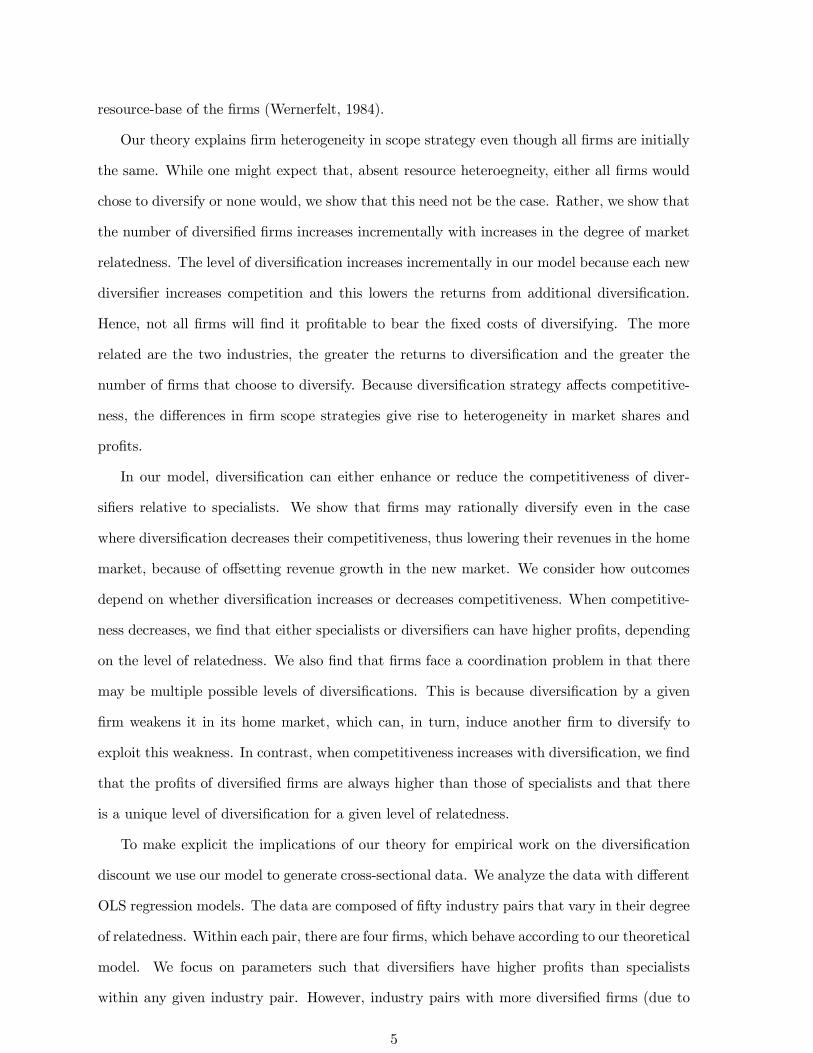
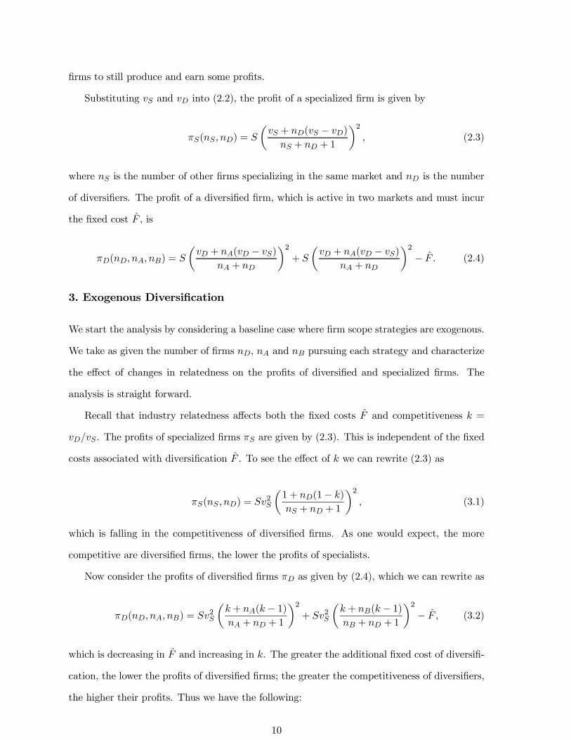
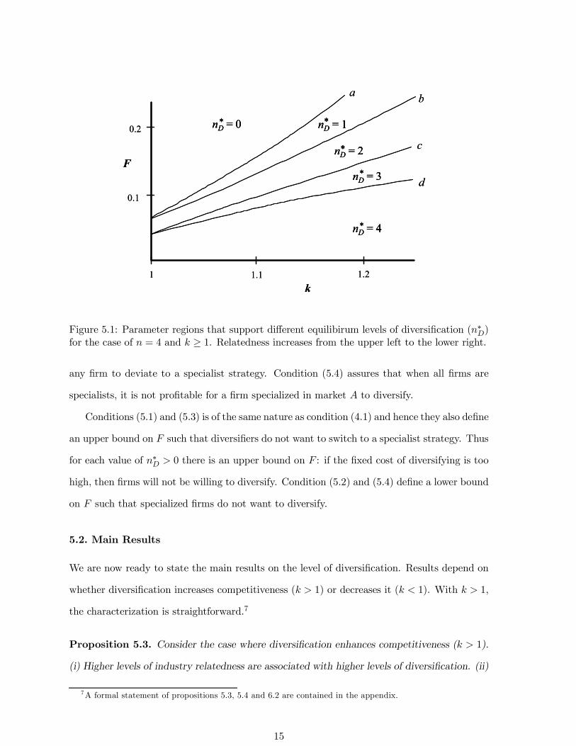
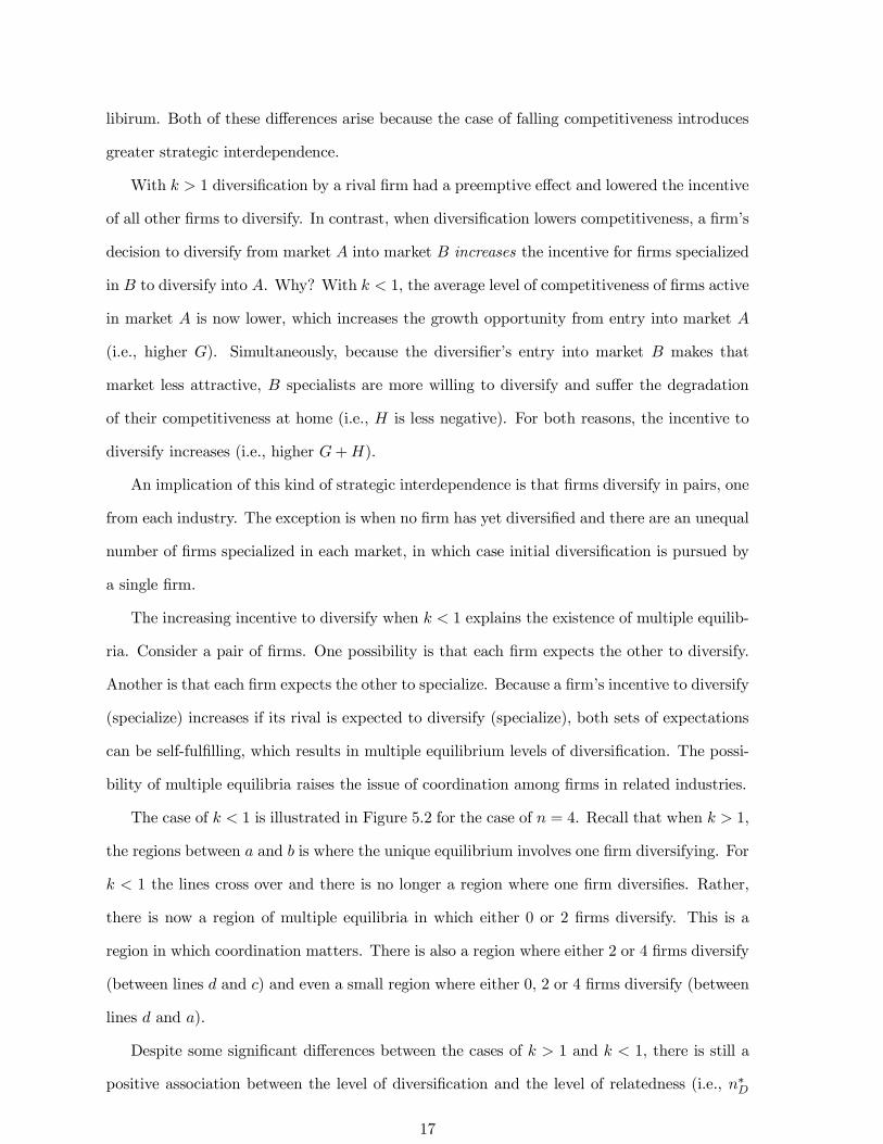
Figure 5.1: Parameter regions that support di¤erent equilibirum levels of diversi…cation (¤)for the case of = 4 and ¸ 1. Relatedness increases from the upper left to the lower right.

any …rm to deviate to a specialist strategy. Condition (5.4) assures that when all …rms are

specialists, it is not pro…table for a …rm specialized in market to diversify.

Conditions (5.1) and (5.3) is of the same nature as condition (4.1) and hence they also de…ne

an upper bound on such that diversi…ers do not want to switch to a specialist strategy. Thus

for each value of ¤ 0 there is an upper bound on : if the …xed cost of diversifying is too

high, then …rms will not be willing to diversify. Condition (5.2) and (5.4) de…ne a lower bound

on such that specialized …rms do not want to diversify.

5.2. Main Results

We are now ready to state the main results on the level of diversi…cation. Results depend on

whether diversi…cation increases competitiveness ( 1) or decreases it ( 1). With 1,

the characterization is straightforward.7

Proposition 5.3. Consider the case where diversi…cation enhances competitiveness ( 1).

(i) Higher levels of industry relatedness are associated with higher levels of diversi…cation. (ii)

7A formal statement of propositions 5.3, 5.4 and 6.2 are contained in the appendix.

15

For any set of parameter values, there is a unique equilibrium level of diversi…cation (except

at boundaries). (iii) Any level of diversi…cation, from no …rms diversifying (¤ = 0) up to and

including all …rms diversifying (¤ = ), can be an equilibrium.

At the core of the results is the fact that while relatedness varies continuously, diversi…ca-

tion is a discrete event. Thus, a given level of diversi…cation is supported by a range of and

values. Figure 5.1 shows the set of and values supporting each level of diversi…cation for

the case of = 4. For example, parameter values falling between lines and are associated

with diversi…cation by two …rms. With 1, there is a unique level of diversi…cation except

for parameter combinations that fall on one of these boundary lines. Increases in relatedness

result in higher and lower . Referring to Figure 5.1, an increase in relatedness involves a

shift from the upper left towards the lower right, which if su¢ciently large, leads to an increase

in the equilibrium level of diversi…cation.

Despite our assumption that all …rms are ex ante identical and have equal access to the

diversi…cation opportunity, we …nd that diversi…cation need not be an all or nothing phenom-

enon. Rather only a subset of …rms may choose to diversify. The reason is that there is a

…xed cost to diversifying and the returns to diversi…cation fall as more …rms diversify. Thus,

for intermediate levels of …xed costs it is economical for only a subset of …rms to diversify.

To what extent do these results hold when diversi…cation decreases competitiveness?

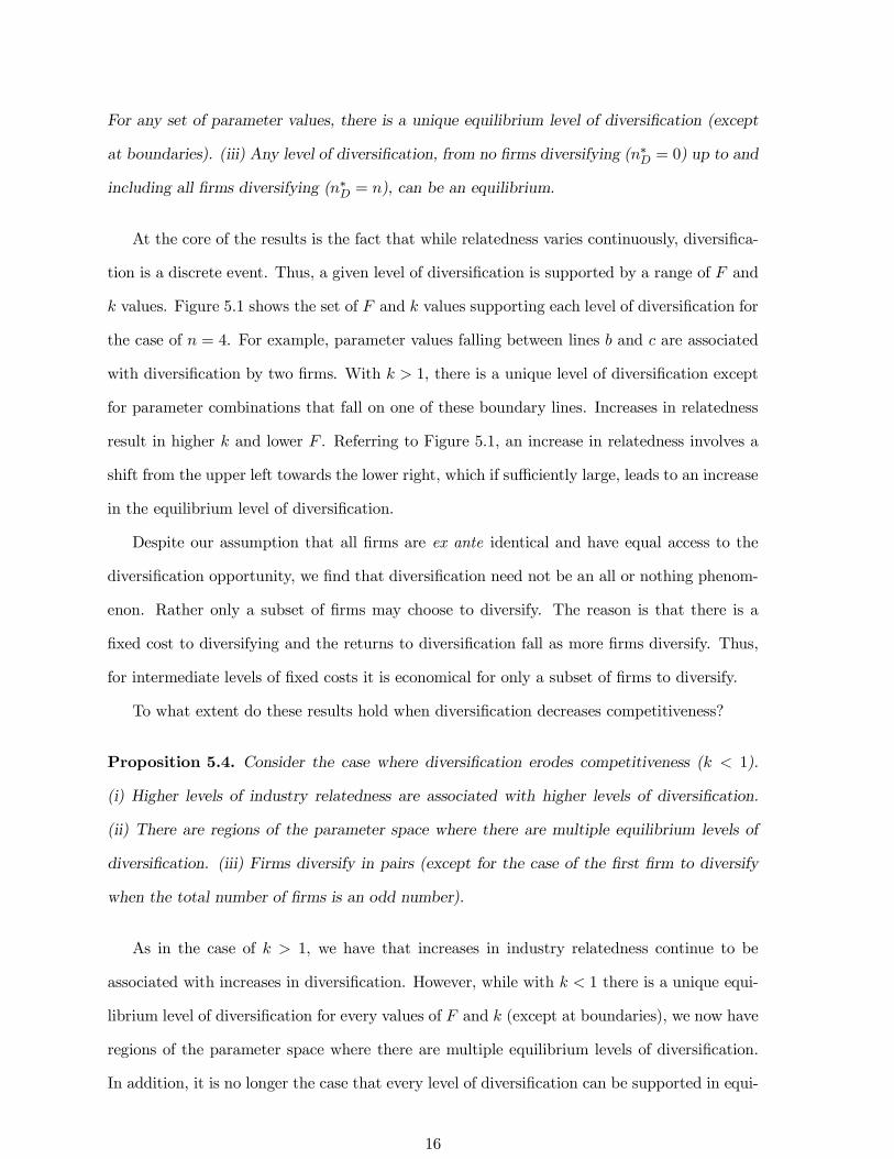
Proposition 5.4. Consider the case where diversi…cation erodes competitiveness ( 1).

(i) Higher levels of industry relatedness are associated with higher levels of diversi…cation.

(ii) There are regions of the parameter space where there are multiple equilibrium levels of

diversi…cation. (iii) Firms diversify in pairs (except for the case of the …rst …rm to diversify

when the total number of …rms is an odd number).

As in the case of 1, we have that increases in industry relatedness continue to be

associated with increases in diversi…cation. However, while with 1 there is a unique equi-

librium level of diversi…cation for every values of and (except at boundaries), we now have

regions of the parameter space where there are multiple equilibrium levels of diversi…cation.

In addition, it is no longer the case that every level of diversi…cation can be supported in equi-

16

libirum. Both of these di¤erences arise because the case of falling competitiveness introduces

greater strategic interdependence.

With 1 diversi…cation by a rival …rm had a preemptive e¤ect and lowered the incentive

of all other …rms to diversify. In contrast, when diversi…cation lowers competitiveness, a …rm’s

decision to diversify from market into market increases the incentive for …rms specialized

in to diversify into . Why? With 1, the average level of competitiveness of …rms active

in market is now lower, which increases the growth opportunity from entry into market

(i.e., higher ). Simultaneously, because the diversi…er’s entry into market makes that

market less attractive, specialists are more willing to diversify and su¤er the degradation

of their competitiveness at home (i.e., is less negative). For both reasons, the incentive to

diversify increases (i.e., higher +).

An implication of this kind of strategic interdependence is that …rms diversify in pairs, one

from each industry. The exception is when no …rm has yet diversi…ed and there are an unequal

number of …rms specialized in each market, in which case initial diversi…cation is pursued by

a single …rm.

The increasing incentive to diversify when 1 explains the existence of multiple equilib-

ria. Consider a pair of …rms. One possibility is that each …rm expects the other to diversify.

Another is that each …rm expects the other to specialize. Because a …rm’s incentive to diversify

(specialize) increases if its rival is expected to diversify (specialize), both sets of expectations

can be self-ful…lling, which results in multiple equilibrium levels of diversi…cation. The possi-

bility of multiple equilibria raises the issue of coordination among …rms in related industries.

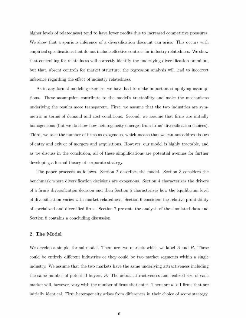
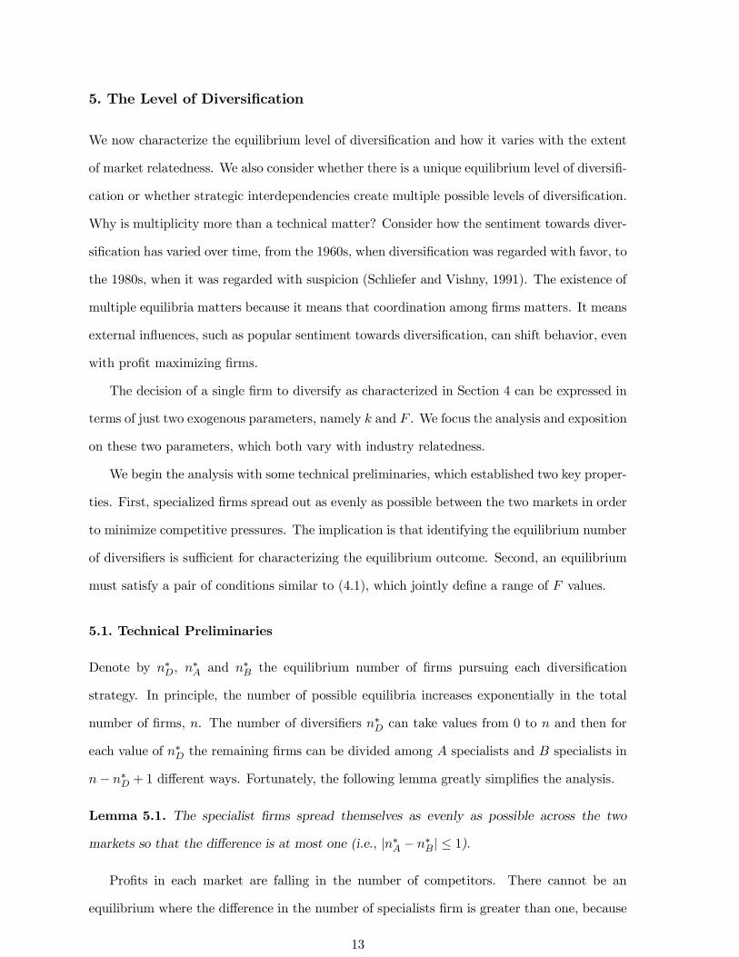
The case of 1 is illustrated in Figure 5.2 for the case of = 4. Recall that when 1,

the regions between and is where the unique equilibrium involves one …rm diversifying. For

1 the lines cross over and there is no longer a region where one …rm diversi…es. Rather,

there is now a region of multiple equilibria in which either 0 or 2 …rms diversify. This is a

region in which coordination matters. There is also a region where either 2 or 4 …rms diversify

(between lines and ) and even a small region where either 0, 2 or 4 …rms diversify (between

lines and ).

Despite some signi…cant di¤erences between the cases of 1 and 1, there is still a

positive association between the level of diversi…cation and the level of relatedness (i.e., ¤

17

10.9 k

F

nD = 4

nD = 0nD = 2

nD = 0 or 2

nD = 2 or 4

nD = 0, 2 or 40.05

*

*

*

*

*

*

dc

ba

10.9 k

F

nD = 4

nD = 0nD = 2

nD = 0 or 2

nD = 2 or 4

nD = 0, 2 or 40.05

*

*

*

*

*

*

dc

ba

Figure 5.2: Parameter regions that support di¤erent equilibirum levels of diversi…cation (¤)for the case of = 4. Relatedness increases from the upper left to the lower right.

increases with shifts from the upper left of Figure 5.2 towards the lower right).

6. Diversi…cation and Pro…ts

When the number of diversi…ed …rms is …xed, greater industry relatedness increases the pro…ts

of diversi…ed …rms while decreasing the pro…ts of specialized …rms, as shown in Proposition 3.1.

However, greater industry relatedness can also trigger an increase in the number of diversi…ed

…rms, as shown in Section 5. Therefore, to fully characterize the e¤ect of relatedness on pro…ts,

we need to characterize the e¤ect of increasing levels of diversi…cation on pro…ts.

Proposition 6.1. (i) For 1, diversi…cation by one …rm decreases the pro…ts of all other

…rms. (ii) For · 1, diversi…cation by one …rm decreases the pro…ts of …rms that are already

diversi…ed (except possibly in the case = = = 1), decreases the pro…ts of …rms that

are specialized in the target market, and weakly increases the pro…ts of …rms specialized in

the diversi…er’s home market.

18

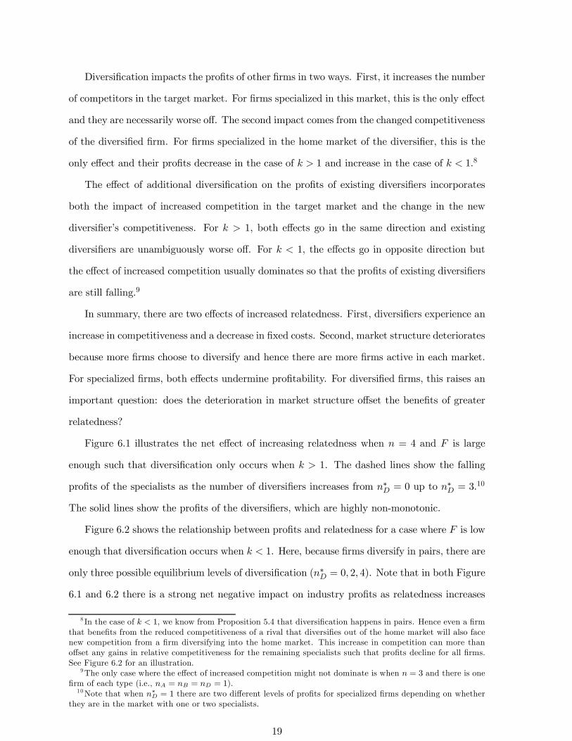
Diversi…cation impacts the pro…ts of other …rms in two ways. First, it increases the number

of competitors in the target market. For …rms specialized in this market, this is the only e¤ect

and they are necessarily worse o¤. The second impact comes from the changed competitiveness

of the diversi…ed …rm. For …rms specialized in the home market of the diversi…er, this is the

only e¤ect and their pro…ts decrease in the case of 1 and increase in the case of 1.8

The e¤ect of additional diversi…cation on the pro…ts of existing diversi…ers incorporates

both the impact of increased competition in the target market and the change in the new

diversi…er’s competitiveness. For 1, both e¤ects go in the same direction and existing

diversi…ers are unambiguously worse o¤. For 1, the e¤ects go in opposite direction but

the e¤ect of increased competition usually dominates so that the pro…ts of existing diversi…ers

are still falling.9

In summary, there are two e¤ects of increased relatedness. First, diversi…ers experience an

increase in competitiveness and a decrease in …xed costs. Second, market structure deteriorates

because more …rms choose to diversify and hence there are more …rms active in each market.

For specialized …rms, both e¤ects undermine pro…tability. For diversi…ed …rms, this raises an

important question: does the deterioration in market structure o¤set the bene…ts of greater

relatedness?

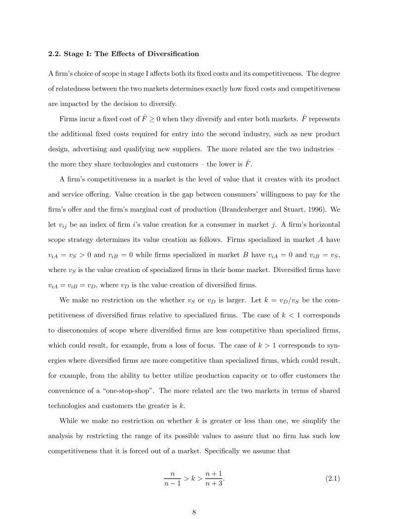
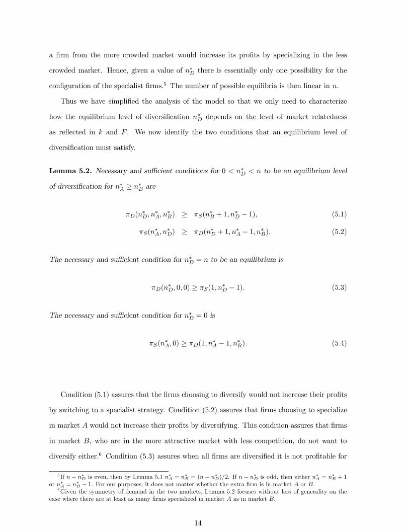
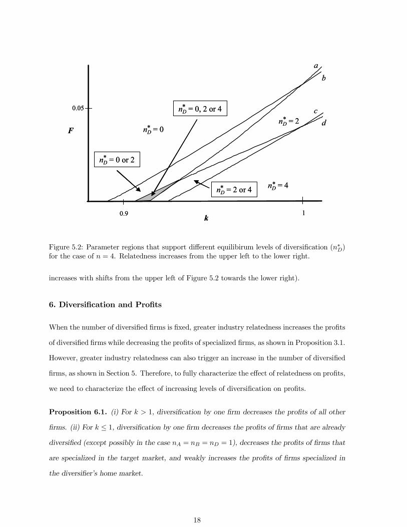
Figure 6.1 illustrates the net e¤ect of increasing relatedness when = 4 and is large

enough such that diversi…cation only occurs when 1. The dashed lines show the falling

pro…ts of the specialists as the number of diversi…ers increases from ¤ = 0 up to ¤ = 3.10

The solid lines show the pro…ts of the diversi…ers, which are highly non-monotonic.

Figure 6.2 shows the relationship between pro…ts and relatedness for a case where is low

enough that diversi…cation occurs when 1. Here, because …rms diversify in pairs, there are

only three possible equilibrium levels of diversi…cation (¤ = 0 2 4). Note that in both Figure

6.1 and 6.2 there is a strong net negative impact on industry pro…ts as relatedness increases

8 In the case of 1, we know from Proposition 5.4 that diversi…cation happens in pairs. Hence even a …rmthat bene…ts from the reduced competitiveness of a rival that diversi…es out of the home market will also facenew competition from a …rm diversifying into the home market. This increase in competition can more thano¤set any gains in relative competitiveness for the remaining specialists such that pro…ts decline for all …rms.See Figure 6.2 for an illustration.

9The only case where the e¤ect of increased competition might not dominate is when = 3 and there is one…rm of each type (i.e., = = = 1).10Note that when ¤ = 1 there are two di¤erent levels of pro…ts for specialized …rms depending on whether

they are in the market with one or two specialists.

19

0.05

0.1

1.0 1.2k

0.0

Profits

0* =Dn

4* =Dn

3* =Dn

2* =Dn

1* =Dn

Profits of diversified firms

Profits of specialized firms

0.05

0.1

1.0 1.2k

0.0

Profits

0* =Dn

4* =Dn

3* =Dn

2* =Dn

1* =Dn

Profits of diversified firms

Profits of specialized firms

Profits of diversified firms

Profits of specialized firms

Figure 6.1: The e¤ect of relatedness () on the equilibrium pro…ts of specialized …rms (dashedlines) and diversi…ed …rms (solid lines) when = 1 and = 4.

0.07

0.1

Profits

0.9 1.0 1.1k

0* =Dn

2* =Dn

4* =Dn

Profits of diversified firms

Profits of specialized firms

0.07

0.1

Profits

0.9 1.0 1.1k

0* =Dn

2* =Dn

4* =Dn

0.07

0.1

Profits

0.9 1.0 1.1k

0* =Dn

2* =Dn

4* =Dn

Profits of diversified firms

Profits of specialized firms

Profits of diversified firms

Profits of specialized firms

Figure 6.2: The e¤ect of relatedness () on the equilibrium pro…ts of specialized …rms (dashedlines) and diversi…ed …rms (solid lines) when = 01 and = 4.

20

and the level of diversi…cation increases. This is a general property of the model, regardless of

whether the increase in relatedness a¤ects competitiveness (as shown in Figures 6.1 and 6.2)

or …xed costs.

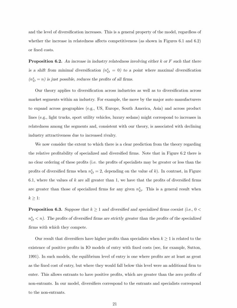
Proposition 6.2. An increase in industry relatedness involving either or such that there

is a shift from minimal diversi…cation (¤ = 0) to a point where maximal diversi…cation

(¤ = ) is just possible, reduces the pro…ts of all …rms.

Our theory applies to diversi…cation across industries as well as to diversi…cation across

market segments within an industry. For example, the move by the major auto manufacturers

to expand across geographies (e.g., US, Europe, South America, Asia) and across product

lines (e.g., light trucks, sport utility vehicles, luxury sedans) might correspond to increases in

relatedness among the segments and, consistent with our theory, is associated with declining

industry attractiveness due to increased rivalry.

We now consider the extent to which there is a clear prediction from the theory regarding

the relative pro…tability of specialized and diversi…ed …rms. Note that in Figure 6.2 there is

no clear ordering of these pro…ts (i.e. the pro…ts of specialists may be greater or less than the

pro…ts of diversi…ed …rms when ¤ = 2, depending on the value of ). In contrast, in Figure

6.1, where the values of are all greater than 1, we have that the pro…ts of diversi…ed …rms

are greater than those of specialized …rms for any given ¤. This is a general result when

¸ 1:

Proposition 6.3. Suppose that ¸ 1 and diversi…ed and specialized …rms coexist (i.e., 0

¤ ). The pro…ts of diversi…ed …rms are strictly greater than the pro…ts of the specialized

…rms with which they compete.

Our result that diversi…ers have higher pro…ts than specialists when ¸ 1 is related to the

existence of positive pro…ts in IO models of entry with …xed costs (see, for example, Sutton,

1991). In such models, the equilibrium level of entry is one where pro…ts are at least as great

as the …xed cost of entry, but where they would fall below this level were an additional …rm to

enter. This allows entrants to have positive pro…ts, which are greater than the zero pro…ts of

non-entrants. In our model, diversi…ers correspond to the entrants and specialists correspond

to the non-entrants.

21

A major di¤erence between our model and IO entry models is that we allow diversi…cation

to a¤ect a …rm’s competitiveness in its home market. When this e¤ect is negative, we show

in Proposition 5.4 that …rms diversify in pairs. The diversifying …rms impose a negative

externality on each other. This additional e¤ect, not present in traditional entry models, is

what causes the pro…ts of diversi…ers to sometimes fall below those of specialists when 1.

Our results linking diversi…cation and pro…ts have implications for the existence of a di-

versi…cation discount or premium. An implication of Proposition 6.3 is that among …rms

competing in a given industry pair, there is a diversi…cation premium as long as 1. On the

other hand, when 1, one can get either a diversi…cation discount or premium. Somewhat

counter intuitively, in our model a diversi…cation discount can only occur when the …xed costs

of diversi…cation ( ) are low such that …rms diversify when 1.

Thus far we have focused on comparisons of specialists and diversi…ers within a given

industry pair. What are the implications for cross sectional data that pool observations across

many di¤erent industry pairs?

7. Simulated Cross-Sectional Data

We now present a simple exercise designed to explore how the linkages that we have identi…ed

among industry relatedness, market structure, diversi…cation decisions, and pro…ts might im-

pact empirical inferences about the relationship between diversi…cation and performance. To

this end we generate cross-sectional data from the model and then consider the results gener-

ated by di¤erent regression speci…cations. The regressions have …rm pro…ts as the dependent

variable and vary in the controls and interactions that they consider.

7.1. Data Generation

We construct the data set as follows. We consider …fty industry pairs that vary in their degree

of relatedness. There are four …rms competing in each industry pair ( = 4). The restriction

to = 4 is to simplifying the coding of the data generation; the underlying theory holds for

any number of …rms. For each industry pair, we generate the equilibrium scope strategies of

the …rms and record the resulting pro…ts, output quantities, the degree of relatedness for the

22

industry pair, and the …rm scope strategies themselves.

The range of industry-pair relatedness is determined as follows. From the theory, for any

given level of …xed costs there is a lower bound on the level of competitiveness () required for

at least one …rm to diversify, and an upper bound beyond which all …rms diversify. We set the

value of …xed costs at = 01 as in Figure 6.1 and then identify the associated lower bound

( = 1044) and upper bound ( = 1173). We construct our sample to begin and end at

values so as to extend this range by 30% above and below these critical cuto¤s.11 We make

our observations at …fty levels of uniformly distributed along this range (i.e., = 1005,

1010. . . , 1215, 1220).12

In our setting, industries only vary along two dimensions: relatedness and market structure.

We do not include controls for the underlying attractiveness of a given industry since, by

construction, all industries are the same in this regard (e.g. the same size parameter and

the same demand function). One can interpret this as a situation where the empiricist has

e¤ectively controlled for di¤erences in the underlying industry attractiveness.

We construct a market structure variable using the weighted average of the Her…ndahl

indexes corresponding to the industries in which a …rm competes. Speci…cally, the market

structure variable associated with …rm is

=

+

X

=1

µ

¶2

+

+

X

µ

¶2

where and are the total output in each market and and are …rm ’s output in

each market.13

Our data thus consist of pro…t levels () for …rms pursuing strategies of diversi…cation

( = 1) and specialization ( = 0) in industries that vary in their level of relatedness (),

where relatedness varies in terms of its e¤ect on competitiveness rather than on …xed costs,

and where we have used a weighted Her…ndahl index () to capture the market structure of

11We also constructed data sets with ranges 10%, 20% and 40% above and below the critical cuto¤s. Thequalitative results were robust in all cases.12For the level of …xed costs that we focus on, diversi…cation only occurs for values of 1. Hence, the

construction of the data is simpli…ed by the fact that there is a unique equilibrium outcome (as long as oneavoids boundaries), as highlighted in Proposition 5.3.13Firm outputs are taken from the Cournot model detailed in Appendix I.

23

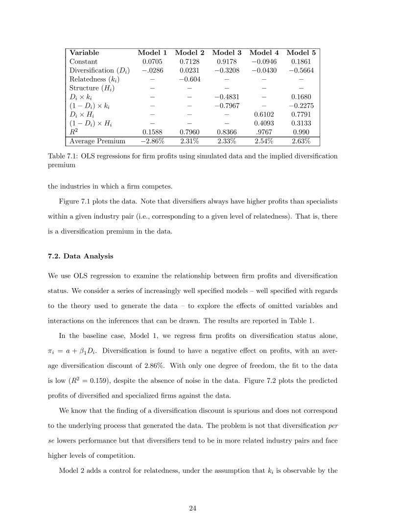
Variable Model 1 Model 2 Model 3 Model 4 Model 5Constant 00705 07128 09178 ¡00946 01861Diversi…cation () ¡0286 00231 ¡03208 ¡00430 ¡05664Relatedness () ¡ ¡0604 ¡ ¡ ¡Structure () ¡ ¡ ¡ ¡ ¡ £ ¡ ¡ ¡04831 ¡ 01680(1¡)£ ¡ ¡ ¡07967 ¡ ¡02275 £ ¡ ¡ ¡ 06102 07791(1¡)£ ¡ ¡ ¡ 04093 031332 01588 07960 08366 9767 0990

Average Premium ¡286% 231% 233% 254% 263%

Table 7.1: OLS regressions for …rm pro…ts using simulated data and the implied diversi…cationpremium

the industries in which a …rm competes.

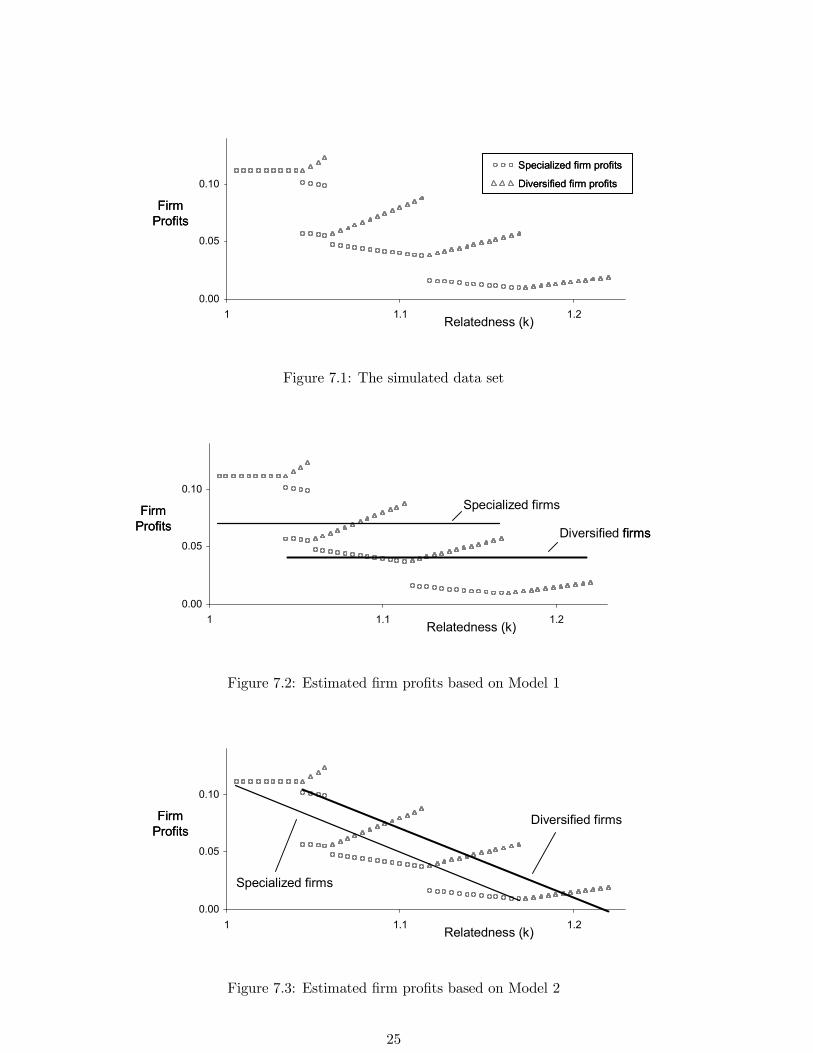
Figure 7.1 plots the data. Note that diversi…ers always have higher pro…ts than specialists

within a given industry pair (i.e., corresponding to a given level of relatedness). That is, there

is a diversi…cation premium in the data.

7.2. Data Analysis

We use OLS regression to examine the relationship between …rm pro…ts and diversi…cation

status. We consider a series of increasingly well speci…ed models – well speci…ed with regards

to the theory used to generate the data – to explore the e¤ects of omitted variables and

interactions on the inferences that can be drawn. The results are reported in Table 1.

In the baseline case, Model 1, we regress …rm pro…ts on diversi…cation status alone,

= + 1. Diversi…cation is found to have a negative e¤ect on pro…ts, with an aver-

age diversi…cation discount of 286%. With only one degree of freedom, the …t to the data

is low (2 = 0159), despite the absence of noise in the data. Figure 7.2 plots the predicted

pro…ts of diversi…ed and specialized …rms against the data.

We know that the …nding of a diversi…cation discount is spurious and does not correspond

to the underlying process that generated the data. The problem is not that diversi…cation per

se lowers performance but that diversi…ers tend to be in more related industry pairs and face

higher levels of competition.

Model 2 adds a control for relatedness, under the assumption that is observable by the

24

0.00

0.05

0.10

1 1.1 1.2Relatedness (k)

FirmProfits

Specialized firm profits

Diversified firm profits

0.00

0.05

0.10

1 1.1 1.2Relatedness (k)

FirmProfits

Specialized firm profits

Diversified firm profits

Specialized firm profits

Diversified firm profits

Figure 7.1: The simulated data set

0.00

0.05

0.10

1 1.1 1.2Relatedness (k)

FirmProfits Diversified firms

Specialized firms

0.00

0.05

0.10

1 1.1 1.2Relatedness (k)

FirmProfits Diversified firms

Specialized firms

Figure 7.2: Estimated …rm pro…ts based on Model 1

0.00

0.05

0.10

1 1.1 1.2Relatedness (k)

FirmProfits

Diversified firms

Specialized firms

0.00

0.05

0.10

1 1.1 1.2Relatedness (k)

FirmProfits

Diversified firms

Specialized firms

Figure 7.3: Estimated …rm pro…ts based on Model 2

25

empiricist:

= + 1 + 2.

Diversi…cation is now found to have a positive e¤ect on pro…ts, with a diversi…cation premium

of 231%. Relatedness is found to have a strongly negative e¤ect on pro…ts (2 = ¡0604). The

…t to the data is much higher (2 = 0796). Figure 7.3 plots the predicted pro…ts of diversi…ed

and specialized …rms against the data. With the control for relatedness, the regression uncovers

the underlying diversi…cation premium. This speci…cation, however, overlooks the fact that

relatedness should have a di¤erential impact on the performance of diversi…ers and specialists.

Model 3 adds an interaction between relatedness and diversi…cation status:

= + 1 + 2 + 3(1¡).

The diversi…cation premium increases to 281%.14 Relatedness is found to have a strongly

negative e¤ects on the pro…ts of all …rms, and the e¤ect is more negative for specialists

(3 = ¡0797) than for diversi…ers (2 = ¡0483). The …t to the data increases marginally

(2 = 0837). Figure 7.4 plots the predicted pro…ts. The reason for the negative e¤ect of

relatedness on the pro…ts of diversi…ed …rms is that relatedness captures both the increas-

ing competitiveness of diversi…ed …rms and the erosion of market structure that comes from

increased levels of diversi…cation.

Model 5 presents a complete speci…cation in which the concentration measure is interacted

with diversi…cation status:

= + 1 + 2 + 3(1¡) + 4 + 5(1¡).

There is a diversi…cation premium of 263%.15 The e¤ect of relatedness is now positive for

diversi…ers (2 = 0168) and negative for specialists (3 = ¡0228). The e¤ect of market

concentration is strongly positive for both diversi…ers (4 = 0780) and for specialists (5 =

14Given the interaction term we calculate the diversi…cation premium as 1 + (2 ¡ 3)¹ where ¹ = 1097 isthe average relatedness in the data set.15We calculate the diversi…cation premium as 1 + (2 ¡ 3)¹+ (4 ¡ 5) ¹ where ¹ = 1097 and ¹ = 0341

is the average weighted Her…ndahl in the data set.

26

0.00

0.05

0.10

1 1.1 1.2Relatedness (k)

FirmProfits

Diversified firms

Specialized firms

0.00

0.05

0.10

1 1.1 1.2Relatedness (k)

FirmProfits

Diversified firms

Specialized firms

Figure 7.4: Estimated pro…ts based on Model 3

0.00

0.05

0.10

1 1.1 1.2Relatedness (k)

FirmProfits

Diversified firms

Specialized firms0.00

0.05

0.10

1 1.1 1.2Relatedness (k)

FirmProfits

Diversified firms

Specialized firms

Figure 7.5: Estimated pro…ts based on Model 4

0.00

0.05

0.10

1 1.1 1.2Relatedness (k)

FirmProfits

Diversified firms

Specialized firms

0.00

0.05

0.10

1 1.1 1.2Relatedness (k)

FirmProfits

Diversified firms

Specialized firms

Figure 7.6: Estimated pro…ts based on Model 5

27

0313). The …t is now almost perfect (2 = 0990). Figure 7.5 plots the predicted pro…ts.

The …nal exercise is to consider the inferences when the empiricist can observe concentration

but not relatedness, which leads to Model 4:

= + 1 + 2 + 3(1¡).

There is a diversi…cation premium of 254%.16. The e¤ect of market concentration is strongly

positive for both diversi…ers (2 = 0610) and for specialists (3 = 0410). The …t is very

high (2 = 0980). Figure 7.6 plots the predicted pro…ts. Note that the …tted lines vary with

relatedness even though it is not controlled for, because concentration varies with related-

ness. Controls for either market relatedness or market structure are su¢cient to uncover the

underlying diversi…cation premium in this data.17

There are two ways to interpret the models with omitted variables. The …rst is that the

variable is literally omitted and the second, is that the operationalization of the variable does

not correspond to the underlying theoretical construct. The operationalization of relatedness

and market structure in empirical studies has proven to be challenging and has generated

considerable debate.

Rumelt’s (1974) original measures of relatedness relied on a partially subjective characteri-

zation of the potential for shared activities and resources across businesses given the industries

in which the …rm competes. Subsequent authors sought to develop less subjective and more

systematic measures by using Standard Industry Classi…cation (SIC) codes for a …rm’s indus-

tries to construct concentric-based (e.g., Montgomery andWernerfelt, 1988) and entropy-based

(e.g., Davis and Duhaime, 1992) measures of relatedness. SIC codes, however, have been crit-

icized as not corresponding to the possibilities for sharing activities and resources (Rumelt,

1982; Robins and Wiersema, 1995, 2003; Villalonga, 2004a). More recent approaches include

using technology ‡ows across markets (Robins and Wiersema, 1995; Bowen and Wiersema,

2005), patent citations (Kim and Kogut, 1996), and the actual patterns of diversi…cation

(Teece et. al., 1994; Bryce and Winter, 2004) to measure relatedness. However a consensus

16We calculate the diversi…cation premium as 1 + (2 ¡ 3) ¹ where ¹ = 0341.17We also ran variations on models 4 and 5 in which the variable is included in the speci…cation but not

interacted with . In both cases, there is a diversi…cation premium and a marginal decline in the 2.

28

does not yet seem to have emerged.

Market structure has been operationalized using the standard concentration measures such

as the Her…ndahl index. Since these measures are usually constructed using data based on

SIC codes, they are subject to similar critiques as SIC-based relatedness measures. Bryce

and Winter (2004:19), for example, note that although most analysts would agree that the

“Paving Mixtures and Blocks” industry and the “Concrete, Ready-Mixed” industry are highly

related, the SIC coding structure treats them as highly unrelated, assigning them to di¤erent

single-digit classi…cations.

The simple exercise in this section elucidates some of what is at stake in the e¤orts to

develop e¤ective control variables. For example, comparing Model 3 and Model 5 shows that

the lack of e¤ective controls for market structure can bias downward estimates on the e¤ects

of relatedness on performance.

8. Conclusion

We address two key debates in the extensive empirical literature on corporate diversi…cation:

the existence of a diversi…cation discount and the relative importance of relatedness and mar-

ket structure for the performance of diversi…ed …rms. We develop a formal theory in which

the decision to diversify is endogenous and a¤ects the both market structure and …rms’ com-

petitiveness. Our key exogenous variable is the extent of industry relatedness.

We decompose the decision to diversify into three key components – the …xed costs of entry,

the growth opportunity and the e¤ect on home-market competitiveness – that all depend on

the degree of industry relatedness. Although we start with homogeneous …rms, heterogeneity

naturally emerges as …rms make di¤erent diversi…cation decisions due to decreasing returns.

As more …rms diversify, the increased number of rivals in each industry reduce the growth

opportunities available to additional diversi…ers. This emergent heterogeneity in …rm scope

strategies leads to heterogeneity in market shares and pro…ts.

Market structure depends on the relative number of …rms that choose to specialize versus

the number that choose to diversify and compete in multiple industries. Because these di-

versi…cation decisions depend on the level of relatedness, we …nd that relatedness and market

29

structure are not distinct constructs in our theory. Within our formal model we make precise

the negative impacts of relatedness on market structure.

We …nd a non-monotonic e¤ect of relatedness on the performance of diversi…ed …rms.

Although greater relatedness increases the competitiveness of diversi…ed …rms, it can also

spur additional diversi…cation and thereby erode market structure and performance. As we

show in the data simulation, overlooking these e¤ects in empirical speci…cations can give rise

to spurious inferences of a diversi…cation discount. The emerging literature on the formal

foundations of strategy has tended to emphasize business-level rather than corporate-level

issues. In this paper, we have sought to expand the scope of inquiry.

Like any model, ours contains many simplifying assumptions such as there being only

two, symmetric markets and initially homogeneous …rms. Our objective, however, is not to

reproduce reality, but rather to elucidate some of the drivers of diversi…cation patterns that

one might see in real markets. Nonetheless, relaxing some of the simplifying assumptions could

form the basis of future research. The simplicity of our model, especially when specialized to

= 2, 3 or 4 …rms, suggests that it could serve as a tractable platform.

Given the importance of resource heterogeneity in the literature, a natural extension would

be to endow some …rms in our model with valuable resources. One could then explore whether

resourced or unresourced …rms have a greater incentive to diversify and how the speci…city

of the resources a¤ects these incentives. By considering more than two markets, one could

address the extent to which a …rm has diversi…ed and possibly elucidate the construction of

measures of relatedness in a …rm’s portfolio of businesses. Finally, one could endogenize the

number of …rms in order to address entry and exit dynamics, possibly involving merger and

acquisition activity.

References

[1] Adner, R. and Zemsky, P. 2005. “Disruptive technology and the emergence of competi-tion,” Rand Journal of Economics, 36(2): 229–254.

[2] Adner, R. and Zemsky, P. 2006. “A demand based perspective on sustainable competitiveadvantage.” Strategic Management Journal 27(3): 215–240.

[3] Amihud, Y., and Lev, B. 1981. “Risk reduction as a managerial motive for conglomeratemergers,” Bell Journal of Economics 12: 605–617.

30

[4] Anso¤, H. I. 1957. “Strategies for diversi…cation,” Harvard Business Review 35(2): 113–124.

[5] Berger, P., and Ofek, E.1995. “Diversi…cation’s e¤ect on …rm value,” Journal of FinancialEconomics 37: 39–65.

[6] Bettis, R. 1981. “Performance di¤erences in related and unrelated diversi…ed …rms,”Strategic Management Journal 2: 379–393.

[7] Bernardo, A., and Chowdhry, B. 2002. “Resources, real options and corporate strategy,”Journal of Financial Economics 63: 211–234.

[8] Bowen, H.P. and Wiersema, M.F. 2005. “Foreign-based competition and corporate diver-si…cation strategy,” Strategic Management Journal 26(12): 1153-1172.

[9] Brandenburger, A. and Stuart, H. W. 1996. “Value-based business strategy,” Journal ofEconomics and Management Strategy 5: 5–24.

[10] Bryce, D.J. and Winter, S.G. 2004. “The Bryce-Winter relatedness index: A new approachfor measuring inter-industry relatedness in strategy research,” mimeo, Wharton School.

[11] Campa, J. M., and Kedia, S. 2002. “Explaining the diversi…cation discount,” Journal ofFinance 57: 1731–1762.

[12] Caves, R. 1971, “International corporations: The industrial economics of foreign invest-ment,” Economica 38: 1–27.

[13] Chatterjee, S. andWernerfelt, B. 1991. “The link between resources and type of diversi…-cation: Theory and evidence,” Strategic Management Journal 12(1): 33–48.

[14] Christensen, H.K. and Montgomery, C. 1981. “Corporate economic performance: Diver-si…cation strategy vs. market structure,” Strategic Management Journal 2(4): 327–343.

[15] Davis, R. and Duhaime, I.M. 1992. “Diversi…cation, vertical integration, and industryanalysis: New perspectives and measurement,” Strategic Management Journal 13(7): 511-524.

[16] Dehejia, R.S. and Wahba, S. 2001. “Propensity score matching methods for non-experimental causal studies,” Review of Economics and Statistics 84: 151–161.

[17] Graham, J. R., Lemmon, M. L. and Wolf, J. G. 2002. “Does corporate diversi…cationdestroy value?” The Journal of Finance 57(2): 695–720.

[18] Gimeno, J. and Woo, C.Y. 1999. “Multimarket contact, economies of scope, and …rmperformance,” Academy of Management Journal 43(3): 239–259.

[19] Gomes, J. and Livdan, D. 2004. “Optimal diversi…cation: Reconciling theory and evi-dence,” The Journal of Finance 59 (2): 507–535.

[20] Heckman, J. 1979. “Sample selection bias as a speci…cation error.” Econometrica 47:153–161.

[21] Jensen, M. 1986. “Agency costs of free cash ‡ow, corporate …nance and takeovers,” Amer-ican Economic Review 76: 323–329.

31

[22] Katz, M. and Shapiro, C. 1985. “Network externalities, competition and compatibility.”American Economic Review 75: 424–440.

[23] Karnani, A. and Wernerfelt, B. 1985. “Multiple point competition,” Strategic ManagementJournal 6: 87–96.

[24] Kim, D. and Kogut, B. 1996. “Technological platforms and diversi…cation,” OrganizationScience 7(3): 283–301.

[25] Lang L, and Stulz R. 1994. “Tobin’s q, corporate diversi…cation, and …rm performance.”Journal of Political Economy 102: 1248–1280.

[26] Levinthal, D. and Wu, B. 2005. “The rational tradeo¤ between corporate scope andpro…tability: the role of capacity-constrained capabilities and market maturity.” mimeo,Wharton School.

[27] Lippman, S. A. and Rumelt, R. P. 2003. “A bargaining perspective on resource advantage”Strategic Management Journal 24(11): 1069–1086.

[28] MacDonald, G. and Ryall M. 2004. “How do value creation and competition determinewhether a …rm appropriates value?” Management Science 50: 1319–1333.

[29] Makadok, R. 2001. “Toward a synthesis of the resource-based and dynamic-capabilityviews of rent creation,” Strategic Management Journal 22(5): 387–401.

[30] Makadok, R., and Barney, J. 2001. “Strategic factor market intelligence: An application ofinformation economics to strategy formulation and competitor intelligence,” ManagementScience 47(12): 1621–1638.

[31] Maksimovic, V. and Phillips, G. 2002. “Do conglomerate …rms allocate resources ine¢-ciently across industries? Theory and evidence” The Journal of Finance 57(2): 721–767.

[32] Martin, J.D. and Sayrak, A. 2003. “Corporate diversi…cation and shareholder value: asurvey of recent literature.” Journal of Finance 9: 37–57.

[33] Matsusaka, J. 2001, “Corporate diversi…cation, value maximization, and organizationalcapabilities,” Journal of Business 74: 409–431.

[34] Montgomery, C. A. 1994. “Corporate diversi…cation,” Journal of Economic Perspectives8(3): 163–178.

[35] Montogmery, C. A. 1985. “Product-market diversi…cation and market power.” Academyof Management Journal 28(4): 789–798.

[36] Montgomery,C.A. and Wernerfelt, B. 1988. “Diversi…cation, Ricardian rents, and Tobin’sq,” RAND Journal of Economics 19(4): 623–632.

[37] Myers, S. and Majluf, N.S. 1984. “Corporate …nancing and investment decisions when…rms have information that investors do not have”, Journal of Financial Economics 13:187–221.

[38] Penrose, E. 1959. The Theory of Growth of the Firm, New York: John Wiley and Sons.

[39] Porter, M.E., 1987. “From competitive advantage to corporate strategy,” Harvard Busi-ness Review May-June: 43–59.

32

[40] Ramanujam, V. and Varadarajan, P. 1989. “Research on corporate diversi…cation: Asynthesis,” Strategic Management Journal 10: 523–551.

[41] Robins, J. and Wiersema, M.F. 1995. “A resource-based approach to the multibusiness…rm: empirical analysis of portfolio interrelationships and corporate …nancial perfor-mance.” Strategic Management Journal 16(4): 277–299.

[42] Robins, J. and Wiersema, M.F. 2003. “The measurement of corporate portfolio strategy:Analysis of the content validity of related diversi…cation indexes,” Strategic ManagementJournal 24(1): 39–59.

[43] Rumelt, R.P., 1974. Strategy, Structure, and Economic Performance, Division of Research,Harvard Business School, Boston, MA.

[44] Rumelt, R.P. 1982. “Diversi…cation strategy and pro…tability,” Strategic ManagementJournal 3: 359–369

[45] Shleifer, A. and Vishny, R.W. 1989, “Managerial entrenchment: The case of manager-speci…c investments,” Journal of Financial Economics 25: 123–139.

[46] Shleifer, A. and Vishny, R.W. 1991. “Takeovers in the ’60s and the ’80s: Evidence andimplications,” Strategic Management Journal 12: 51–59.

[47] Stern, I. and Henderson, A.D. 2004. “Within-business diversi…cation in technology-intensive industries,” Strategic Management Journal 25(5): 487–505.

[48] Sutton, J. 1991. Sunk Costs and Market Structure: Price Competition, Advertising, andthe Evolution of Concentration. MIT Press, Cambridge: MA.

[49] Teece, D.J., Rumelt, R.P., Dosi, G. and Winter, S.G. 1994. “Understanding corporatecoherence: Theory and evidence,” Journal of Economic Behavior and Organization 23:1–30.

[50] Villalonga, B. 2003. “Research roundtable discussion: The diversi…cation discount.” FEN-Educator Series, www.ssrn.com.

[51] Villalonga, B. 2004a. “Diversi…cation discount or premium? New evidence from the busi-ness information tracking series,” Journal of Finance 59(2): 475–502.

[52] Villalonga, B. 2004b. “Does diversi…cation cause the ‘diversi…cation discount’?” FinancialManagement 33(2): 5–27.

[53] Wernerfelt, B. 1984. "A resource-based view of the …rm," Strategic Management Journal5: 171–180.

[54] Vives, X. 1999. Oligopoly Pricing: Old ideas and New Tools. MIT Press, Cambridge: MA.

9. Appendix I: Cournot Competition

This Appendix fully speci…es the Cournot model that generates the pro…ts given by (2.2) andderives the bounds on given by (2.1) such that this pro…t expression is valid for any choiceof scope strategy by the …rms.

33

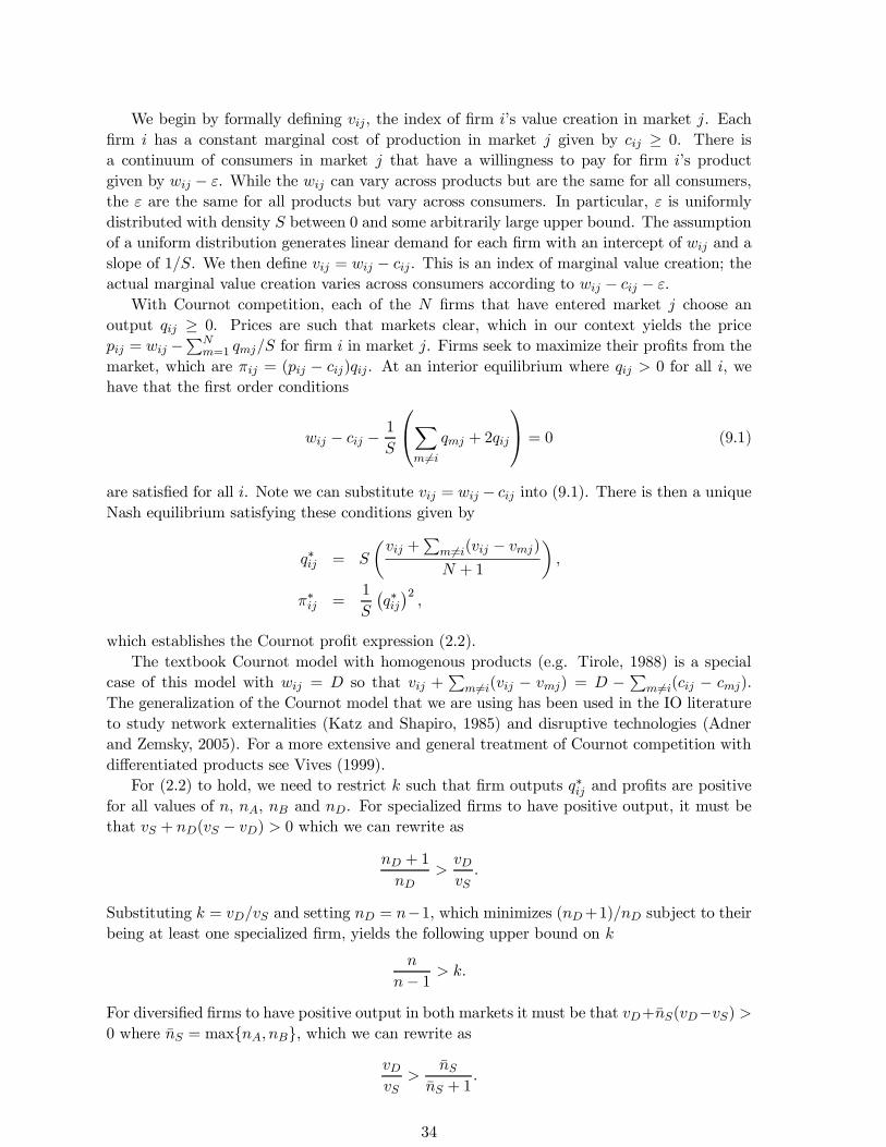
We begin by formally de…ning , the index of …rm ’s value creation in market . Each…rm has a constant marginal cost of production in market given by ¸ 0. There isa continuum of consumers in market that have a willingness to pay for …rm ’s productgiven by ¡ . While the can vary across products but are the same for all consumers,the are the same for all products but vary across consumers. In particular, is uniformlydistributed with density between 0 and some arbitrarily large upper bound. The assumptionof a uniform distribution generates linear demand for each …rm with an intercept of and aslope of 1. We then de…ne = ¡ . This is an index of marginal value creation; theactual marginal value creation varies across consumers according to ¡ ¡ .

With Cournot competition, each of the …rms that have entered market choose anoutput ¸ 0. Prices are such that markets clear, which in our context yields the price = ¡

P=1 for …rm in market . Firms seek to maximize their pro…ts from the

market, which are = ( ¡ ). At an interior equilibrium where 0 for all , wehave that the …rst order conditions

¡ ¡1

0

@X

6= + 2

1

A = 0 (9.1)

are satis…ed for all . Note we can substitute = ¡ into (9.1). There is then a uniqueNash equilibrium satisfying these conditions given by

¤ =

µ +

P 6=( ¡ )

+ 1

¶,

¤ =1

¡¤¢2 ,

which establishes the Cournot pro…t expression (2.2).The textbook Cournot model with homogenous products (e.g. Tirole, 1988) is a special

case of this model with = so that +P

6=( ¡ ) = ¡P

6=( ¡ ).The generalization of the Cournot model that we are using has been used in the IO literatureto study network externalities (Katz and Shapiro, 1985) and disruptive technologies (Adnerand Zemsky, 2005). For a more extensive and general treatment of Cournot competition withdi¤erentiated products see Vives (1999).

For (2.2) to hold, we need to restrict such that …rm outputs ¤ and pro…ts are positivefor all values of , , and . For specialized …rms to have positive output, it must bethat + ( ¡ ) 0 which we can rewrite as

+ 1

.

Substituting = and setting = ¡1, which minimizes (+1) subject to theirbeing at least one specialized …rm, yields the following upper bound on

¡ 1 .

For diversi…ed …rms to have positive output in both markets it must be that +¹(¡) 0 where ¹ = maxf g, which we can rewrite as

¹

¹ + 1.

34

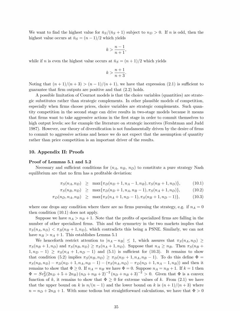
We want to …nd the highest value for ¹(¹ + 1) subject to 0. If is odd, then thehighest value occurs at ¹ = (¡ 1)2 which yields

¡ 1

+ 1,

while if is even the highest value occurs at ¹ = (+ 1)2 which yields

+ 1

+ 3.

Noting that ( + 1)( + 3) ( ¡ 1)( + 1), we have that expression (2.1) is su¢cient toguarantee that …rm outputs are positive and that (2.2) holds.

A possible limitation of Cournot models is that the choice variables (quantities) are strate-gic substitutes rather than strategic complements. In other plausible models of competition,especially when …rms choose prices, choice variables are strategic complements. Such quan-tity competition in the second stage can drive results in two-stage models because it meansthat …rms want to take aggressive actions in the …rst stage in order to commit themselves tohigh output levels; see for example the literature on strategic incentives (Fershtman and Judd1987). However, our theory of diversi…cation is not fundamentally driven by the desire of …rmsto commit to aggressive actions and hence we do not expect that the assumption of quantityrather than price competition is an important driver of the results.

10. Appendix II: Proofs

Proof of Lemmas 5.1 and 5.2Necessary and su¢cient conditions for (, , ) to constitute a pure strategy Nash

equilibrium are that no …rm has a pro…table deviation:

( ) ¸ maxf( + 1 ¡ 1 ) ( + 1 )g, (10.1)

( ) ¸ maxf( + 1 ¡ 1) ( + 1 )g, (10.2)

( ) ¸ maxf( + 1 ¡ 1) ( + 1 ¡ 1)g, (10.3)

where one drops any condition where there are no …rms pursuing the strategy, e.g. if = 0

then condition (10.1) does not apply.Suppose we have + 1. Note that the pro…ts of specialized …rms are falling in the

number of other specialized …rms. This and the symmetry in the two markets implies that( ) ( + 1 ), which contradicts this being a PSNE. Similarly, we can nothave + 1. This establishes Lemma 5.1

We henceforth restrict attention to j ¡ j · 1, which assures that ( ) ¸( + 1 ) and ( ) ¸ ( + 1 ). Suppose that ¸ . Then ( +

1 ¡ 1) ¸ ( + 1 ¡ 1) and (5.1) is su¢cient for (10.3). It remains to showthat condition (5.2) implies ( ) ¸ ( + 1 ¡ 1). To do this de…ne © =

( ) ¡ ( + 1 ¡ 1) ¡ (( ) ¡ ( + 1 ¡ 1 )) and then itremains to show that © ¸ 0. If = we have © = 0. Suppose = + 1. If = 1 then© = 2(2 + 5 + 2) ( + + 2)¡2 ( + + 3)¡2 0. Given that © is a convexfunction of , it remains to show that © ¸ 0 for extreme values of . From (2.1) we havethat the upper bound on is ( ¡ 1) and the lower bound on is ( + 1)( + 3) where = + 2 + 1. With some tedious but straightforward calculations, we have that © 0

35

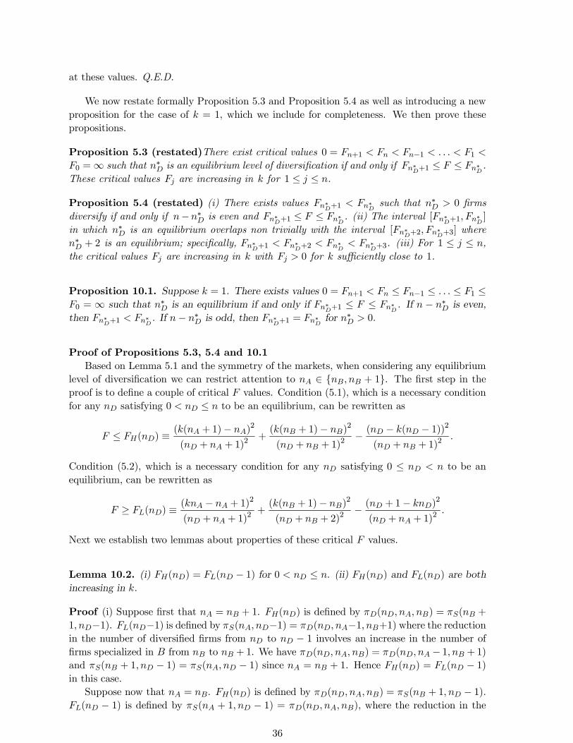
at these values. Q.E.D.

We now restate formally Proposition 5.3 and Proposition 5.4 as well as introducing a newproposition for the case of = 1, which we include for completeness. We then prove thesepropositions.

Proposition 5.3 (restated)There exist critical values 0 = +1 ¡1 1

0 =1 such that ¤ is an equilibrium level of diversi…cation if and only if ¤+1 · · ¤ .These critical values are increasing in for 1 · · .

Proposition 5.4 (restated) (i) There exists values ¤+1 ¤ such that ¤ 0 …rmsdiversify if and only if ¡¤ is even and ¤+1 · · ¤ . (ii) The interval [¤+1 ¤ ]in which ¤ is an equilibrium overlaps non trivially with the interval [¤+2 ¤+3] where¤ + 2 is an equilibrium; speci…cally, ¤+1 ¤+2 ¤ ¤+3. (iii) For 1 · · ,the critical values are increasing in with 0 for su¢ciently close to 1.

Proposition 10.1. Suppose = 1. There exists values 0 = +1 · ¡1 · · 1 ·0 = 1 such that ¤ is an equilibrium if and only if ¤+1 · · ¤ . If ¡ ¤ is even,then ¤+1 ¤ . If ¡ ¤ is odd, then ¤+1 = ¤ for

¤ 0.

Proof of Propositions 5.3, 5.4 and 10.1Based on Lemma 5.1 and the symmetry of the markets, when considering any equilibrium

level of diversi…cation we can restrict attention to 2 f + 1g. The …rst step in theproof is to de…ne a couple of critical values. Condition (5.1), which is a necessary conditionfor any satisfying 0 · to be an equilibrium, can be rewritten as

· () ´(( + 1)¡ )

2

( + + 1)2+

(( + 1)¡ )2

( + + 1)2¡ ( ¡ ( ¡ 1))2

( + + 1)2.

Condition (5.2), which is a necessary condition for any satisfying 0 · to be anequilibrium, can be rewritten as

¸ () ´( ¡ + 1)2

( + + 1)2+

(( + 1)¡ )2

( + + 2)2¡ ( + 1¡ )

2

( + + 1)2.

Next we establish two lemmas about properties of these critical values.

Lemma 10.2. (i) () = ( ¡ 1) for 0 · . (ii) () and () are bothincreasing in .

Proof (i) Suppose …rst that = + 1. () is de…ned by ( ) = ( +

1 ¡1). (¡1) is de…ned by ( ¡1) = ( ¡1 +1) where the reductionin the number of diversi…ed …rms from to ¡ 1 involves an increase in the number of…rms specialized in from to + 1. We have ( ) = ( ¡ 1 + 1)

and ( + 1 ¡ 1) = ( ¡ 1) since = + 1. Hence () = ( ¡ 1)

in this case.Suppose now that = . () is de…ned by ( ) = ( + 1 ¡ 1).

( ¡ 1) is de…ned by ( + 1 ¡ 1) = ( ), where the reduction in the

36

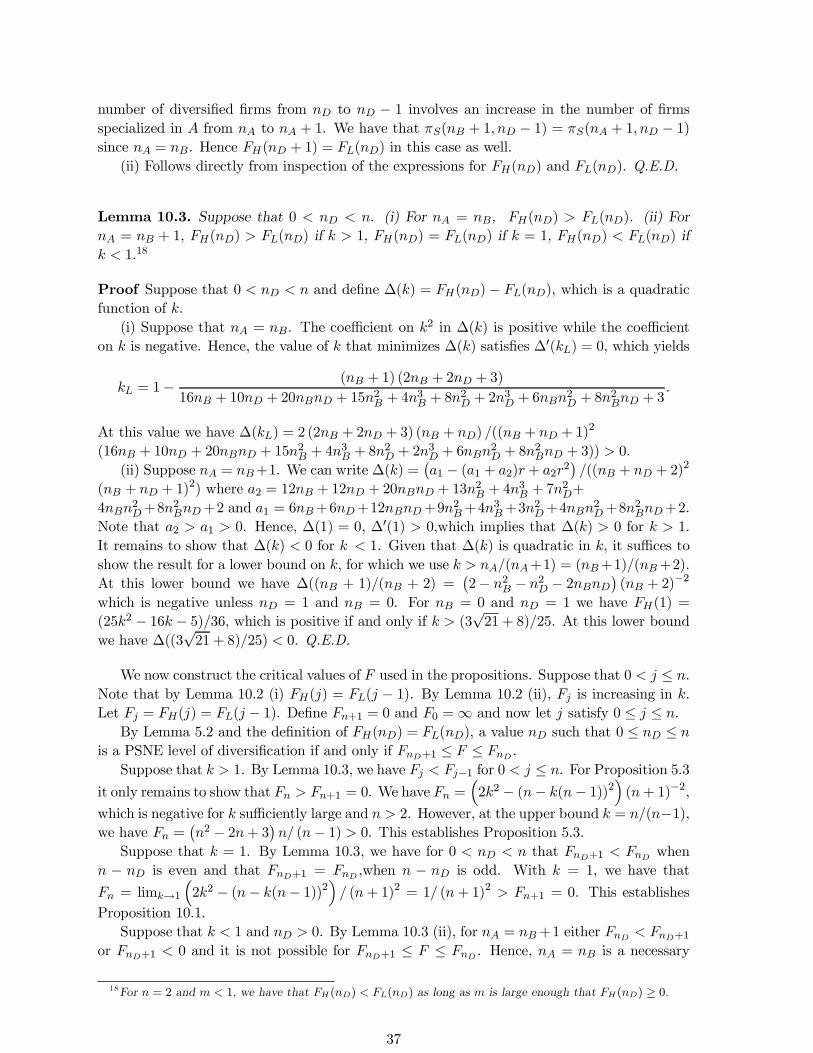
number of diversi…ed …rms from to ¡ 1 involves an increase in the number of …rmsspecialized in from to + 1. We have that ( + 1 ¡ 1) = ( + 1 ¡ 1)

since = . Hence ( + 1) = () in this case as well.(ii) Follows directly from inspection of the expressions for () and (). Q.E.D.

Lemma 10.3. Suppose that 0 . (i) For = , () (). (ii) For = + 1, () () if 1, () = () if = 1, () () if 1.18

Proof Suppose that 0 and de…ne ¢() = ()¡ (), which is a quadraticfunction of .

(i) Suppose that = . The coe¢cient on 2 in ¢() is positive while the coe¢cienton is negative. Hence, the value of that minimizes ¢() satis…es ¢0() = 0, which yields

= 1¡ ( + 1) (2 + 2 + 3)

16 + 10 + 20 + 152 + 43 + 82 + 23 + 62 + 82 + 3.

At this value we have ¢() = 2 (2 + 2 + 3) ( + ) (( + + 1)2

(16 + 10 + 20 + 152 + 43 + 82 + 23 + 62 + 82 + 3)) 0.

(ii) Suppose = +1. We can write ¢() =¡1 ¡ (1 + 2) + 2

2¢(( + + 2)2

( + + 1)2) where 2 = 12 + 12 + 20 + 132 + 43 + 72+

42+82+2 and 1 = 6+6+12+92+43+32+4

2+82+2.

Note that 2 1 0. Hence, ¢(1) = 0, ¢0(1) 0which implies that ¢() 0 for 1.It remains to show that ¢() 0 for 1. Given that ¢() is quadratic in , it su¢ces toshow the result for a lower bound on , for which we use (+1) = (+1)(+2).At this lower bound we have ¢(( + 1)( + 2) =

¡2¡ 2 ¡ 2 ¡ 2

¢( + 2)¡2

which is negative unless = 1 and = 0. For = 0 and = 1 we have (1) =

(252 ¡ 16 ¡ 5)36 which is positive if and only if (3p21 + 8)25. At this lower bound

we have ¢((3p21 + 8)25) 0. Q.E.D.

We now construct the critical values of used in the propositions. Suppose that 0 · .Note that by Lemma 10.2 (i) () = ( ¡ 1). By Lemma 10.2 (ii), is increasing in .Let = () = ( ¡ 1). De…ne +1 = 0 and 0 =1 and now let satisfy 0 · · .

By Lemma 5.2 and the de…nition of () = (), a value such that 0 · ·

is a PSNE level of diversi…cation if and only if +1 · · .Suppose that 1. By Lemma 10.3, we have ¡1 for 0 · . For Proposition 5.3

it only remains to show that +1 = 0. We have =³22 ¡ (¡ (¡ 1))2

´(+ 1)¡2,

which is negative for su¢ciently large and 2. However, at the upper bound = (¡1),we have =

¡2 ¡ 2+ 3

¢ (¡ 1) 0. This establishes Proposition 5.3.

Suppose that = 1. By Lemma 10.3, we have for 0 that +1 when ¡ is even and that +1 = ,when ¡ is odd. With = 1, we have that

= lim!1

³22 ¡ (¡ (¡ 1))2

´ (+ 1)2 = 1 (+ 1)2 +1 = 0. This establishes

Proposition 10.1.Suppose that 1 and 0. By Lemma 10.3 (ii), for = +1 either +1

or +1 0 and it is not possible for +1 · · . Hence, = is a necessary

18For = 2 and 1, we have that () () as long as is large enough that () ¸ 0.

37

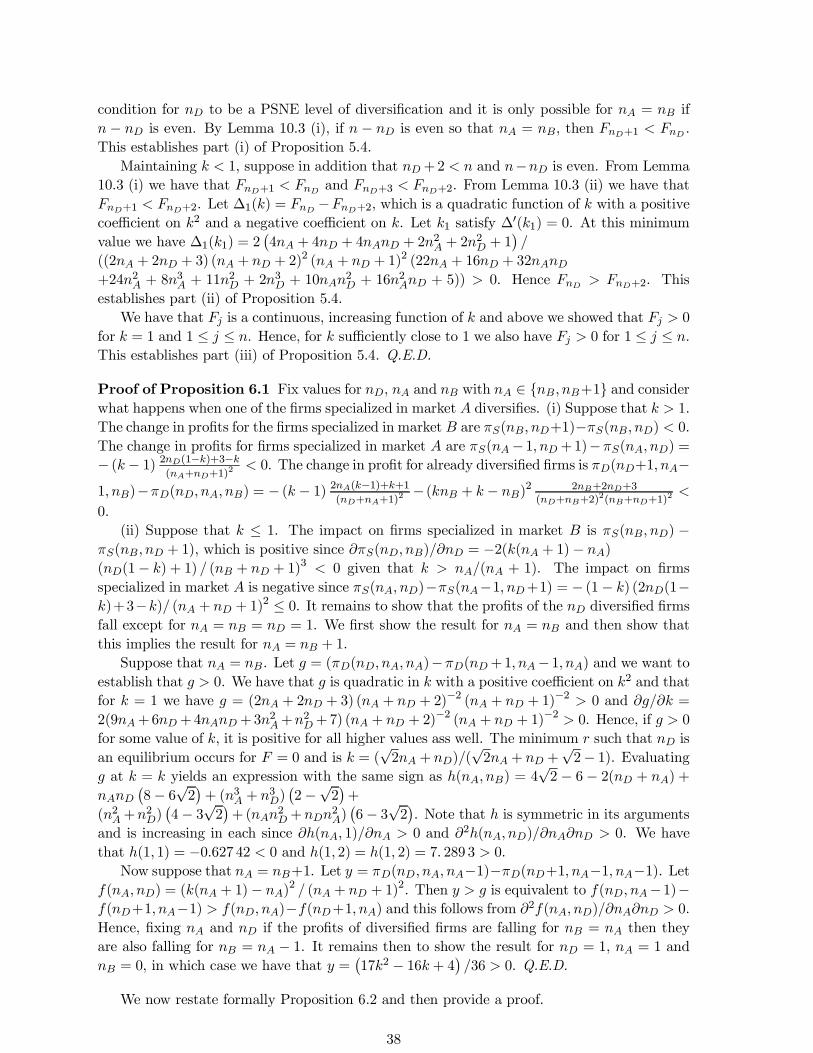
condition for to be a PSNE level of diversi…cation and it is only possible for = if ¡ is even. By Lemma 10.3 (i), if ¡ is even so that = , then +1 .This establishes part (i) of Proposition 5.4.

Maintaining 1, suppose in addition that +2 and ¡ is even. From Lemma10.3 (i) we have that +1 and +3 +2. From Lemma 10.3 (ii) we have that+1 +2. Let ¢1() = ¡+2, which is a quadratic function of with a positivecoe¢cient on 2 and a negative coe¢cient on . Let 1 satisfy ¢0(1) = 0. At this minimumvalue we have ¢1(1) = 2

¡4 + 4 + 4 + 22 + 22 + 1

¢

((2 + 2 + 3) ( + + 2)2 ( + + 1)2 (22 + 16 + 32+242 + 83 + 112 + 23 + 10

2 + 162 + 5)) 0. Hence +2. This

establishes part (ii) of Proposition 5.4.We have that is a continuous, increasing function of and above we showed that 0

for = 1 and 1 · · . Hence, for su¢ciently close to 1 we also have 0 for 1 · · .This establishes part (iii) of Proposition 5.4. Q.E.D.

Proof of Proposition 6.1 Fix values for , and with 2 f +1g and considerwhat happens when one of the …rms specialized in market diversi…es. (i) Suppose that 1.The change in pro…ts for the …rms specialized in market are ( +1)¡( ) 0.The change in pro…ts for …rms specialized in market are (¡1 +1)¡( ) =

¡ ( ¡ 1) 2(1¡)+3¡(++1)

2 0. The change in pro…t for already diversi…ed …rms is (+1 ¡

1 )¡( ) = ¡ ( ¡ 1) 2(¡1)++1(++1)

2 ¡ ( + ¡ )2 2+2+3(++2)

2(++1)2

0.(ii) Suppose that · 1. The impact on …rms specialized in market is ( ) ¡

( + 1), which is positive since ( ) = ¡2(( + 1)¡ )

((1¡ ) + 1) ( + + 1)3 0 given that ( + 1). The impact on …rmsspecialized in market is negative since ( )¡(¡1 +1) = ¡ (1¡ ) (2(1¡)+3¡) ( + + 1)2 · 0. It remains to show that the pro…ts of the diversi…ed …rmsfall except for = = = 1. We …rst show the result for = and then show thatthis implies the result for = + 1.

Suppose that = . Let = (( )¡(+1 ¡1 ) and we want toestablish that 0. We have that is quadratic in with a positive coe¢cient on 2 and thatfor = 1 we have = (2 + 2 + 3) ( + + 2)¡2 ( + + 1)¡2 0 and =

2(9+6+4+32+2+7) ( + + 2)¡2 ( + + 1)¡2 0. Hence, if 0

for some value of , it is positive for all higher values ass well. The minimum such that isan equilibrium occurs for = 0 and is = (

p2 + )(

p2 + +

p2¡ 1). Evaluating

at = yields an expression with the same sign as ( ) = 4p2 ¡ 6¡ 2( + ) +

¡8¡ 6

p2¢+ (3 + 3)

¡2¡

p2¢+

(2+2)¡4¡ 3

p2¢+(

2+

2)¡6¡ 3

p2¢. Note that is symmetric in its arguments

and is increasing in each since ( 1) 0 and 2( ) 0. We havethat (1 1) = ¡0627 42 0 and (1 2) = (1 2) = 7 289 3 0.

Now suppose that = +1. Let = ( ¡1)¡(+1 ¡1 ¡1). Let( ) = (( + 1)¡ )

2 ( + + 1)2. Then is equivalent to ( ¡1)¡(+1 ¡1) ( )¡(+1 ) and this follows from 2( ) 0.Hence, …xing and if the pro…ts of diversi…ed …rms are falling for = then theyare also falling for = ¡ 1. It remains then to show the result for = 1, = 1 and = 0, in which case we have that =

¡172 ¡ 16 + 4

¢36 0. Q.E.D.

We now restate formally Proposition 6.2 and then provide a proof.

38

Proposition 6.2 (restated) (i) Let 1 0 be such that ¤ = 0 is an equilibriumi¤ ¸ 1 and ¤ = is an equilibrium i¤ · . Decreasing from ¸ 1 downto = and thereby shifting from minimal to maximal diversi…cation causes a fall in thepro…ts of all …rms.(ii) Let 1 (¡ 1) be such that ¤ = 0 is an equilibrium i¤ · 1 and ¤ = isan equilibrium i¤ ¸ . Increasing from · 1 up to = and thereby shifting fromminimal to maximal diversi…cation causes a fall in the pro…ts of all …rms.

Proof of Proposition 6.2 (i) Suppose that = () ¸ 0. For large we have that thepro…ts of all …rms are (2 0) if is even and ((¡ 1)2 0) and ((+ 1)2 0) if isodd. We have ((¡ 1)2 0) (2 0) ((+ 1)2 0) = 4 (+ 3)2 and we focus onthe lower bound. The pro…ts when = are ( 0 0) = 22(+1)2 ¡ . The largest such that = is an equilibrium is () = 22 (+ 1)2 ¡ (¡ (¡ 1))2 (+ 1)2 andat this we have ( 0 0) = (¡ (¡ 1))2 (+ 1)2, which is falling in . The lowest such that () ¸ 0 is =

¡¡ 1¡

p2¢(2 ¡ 1 ¡ 2) and at this lower limit we have

(+12 0)¡ ( 0 0) = (4 (+ 3)2 ¡ (¡ (¡ 1))2

(+ 1)2) = 2¡¡

p2¢ ¡2 + 3

p2 + 5

¡p2¡ 1

¢¡ 4¢(¡ 1) (+ 1)¡2 (+ 3)¡2

¡+

p2¡ 1

¢¡2 0.

(ii) Suppose that is su¢ciently low that all …rms are specialized. Pro…ts are at least(( + 1)2 0) = 4 (+ 3)2. Pro…ts of the …rms when = are ( 0 0). Wehave = , which is de…ned by ( 0 0) = (1 ¡ 1) = (¡ (¡ 1))2 (+ 1)2 andhence the di¤erence in pro…ts are 4 (+ 3)2 ¡ (¡ (¡ 1))2 (+ 1)2 which is increasingin . How low can be? This occurs for = 0 in which case satis…es 22 (+ 1)2 =

(¡ (¡ 1))2 (+ 1)2, which yields ¸¡¡ 1¡

p2¢(2 ¡ 2 ¡ 1) and at this lower

bound we have that 4 (+ 3)2 ¡ (¡ (¡ 1))2 (+ 1)2 = 2¡+

p2¡ 1

¢¡2(+ 3)¡2

(+ 1)¡2¡¡

p2¢(2 ¡ 4 + 3

p2 + 5

¡p2¡ 1

¢) (¡ 1) 0. Q.E.D.

Proof of Proposition 6.3Suppose we have an equilibrium where 2 f + 1g and 0 . From (5.1)

we have that ( ) ¸ ( + 1 ¡ 1). For ¸ 1, we have that ( +

1 ¡ 1) ( ). Since ¸ we have that ( ) ¸ ( ). Hence thepro…t of diversi…ed …rms, ( ), is strictly greater than the pro…ts specialized …rms,( ) and ( ). Q.E.D.

39