Diverse Classifiers for NLP Disambiguation Tasks

Comparison, Optimization, Combination, and Evolution

Jakub Zavrel ♣ Sven Degroeve ♦ Anne Kool ♣Walter Daelemans ♣Kristiina Jokinen ♦

♣ CNTS - Language Technology Group, University of Antwerp{zavrel|kool|daelem}@uia.ua.ac.be

♦ Center for Evolutionary Language Engineering, Ieper, Belgium{sven.degroeve|kristiina.jokinen}@sail.com

Abstract

In this paper we report preliminary results from an ongoing study that investigates the perfor-mance of machine learning classifiers on a diverse set of Natural Language Processing (NLP)tasks. First, we compare a number of popular existing learning methods (Neural networks,Memory-based learning, Rule induction, Decision trees, Maximum Entropy, Winnow Per-ceptrons, Naive Bayes and Support Vector Machines), and discuss their properties vis a vistypical NLP data sets. Next, we turn to methods to optimize the parameters of single learningmethods through cross-validation and evolutionary algorithms. Then we investigate how wecan get the best of all single methods through combination of the tested systems in classifierensembles. Finally we discuss new and more thorough methods of automatically constructingensembles of classifiers based on the techniques used for parameter optimization.

Keywords: Models and algorithms for computational neural architectures

1 Introduction

In recent years the field of Natural Language Processing (NLP) has been radically transformed bya switch from a deductive methodology (i.e. explaining data from theories or models constructedmanually) to an inductive methodology (i.e. deriving models and theories from data) (see e.g. Ab-ney (1996) for a review). An important component of this transformation is the realization thatmany NLP tasks can be modeled as simple classification tasks or as ensembles of simple classi-fiers (Daelemans, 1996; Ratnaparkhi, 1997). Thus NLP has been able to capitalize on a largebody of research in the field of machine learning and statistical modeling. This, accompanied bythe continuing explosion of computer power, storage size, and availability of training corpora, haslead to increasingly accurate language models for a quickly growing number of language modelingtasks. However, which machine learning methods have the best performance on NLP data sets isstill an active area of research.

In this paper, we empirically study the performance of a range of supervised learning techniqueson a selection of benchmark tasks in NLP. In classification-based, supervised learning, a learn-ing algorithm constructs a classifier for a task by processing a set of examples. Each exampleassociates a feature vector (the problem description) with one of a finite number of classes (thesolution). Given a new feature vector, the classifier assigns a class to the problem description itrepresents by means of extrapolation from a “knowledge structure” extracted from the examples.Different learning algorithms construct different types of knowledge representations: probabilitydistributions, decision trees, rules, exemplars, weight vectors, etc.

Classification-based supervised learning methods seem to be especially well suited for NLPtasks because they fit the main task in all areas of NLP very well: implementing a complex,context-sensitive, mapping between different levels of linguistic representation. Sub-tasks in such

a transformation can be of two types (Daelemans, 1996): segmentation (e.g. decide whether aword or tag is the start or end of an NP), and disambiguation (e.g. decide whether a word is anoun or a verb). We can even carve up complex NLP tasks like syntactic analysis into a numberof such classification tasks with input vectors representing a focus item and a dynamically selectedsurrounding context. Output of one classifier (e.g. a tagger or a chunker) is then used as input byother classifiers (e.g. syntactic relation assignment).

Although the existence of machine learning data repositories (such as UCI (Blake et al., 1998))has made it easy to compare and benchmark machine learning algorithms, such studies (e.g. Michieet al., 1994) have not usually focused on natural language learning. However, language data setshave characteristics that make them quite different from typical machine learning data sets:

• Size: Millions of example cases, large numbers of features, many of which redundant orirrelevant, and very large numbers of feature values (e.g. all words of a lexicon). This placesa high computational burden on many existing learning algorithms.

• Disjunctiveness: Language is characterized by an interplay between rules, (sub)regularities,and exceptions. Even exceptions (that are difficult to distinguish from noise) can be membersof small but productive families. Daelemans et al. (1999) have observed that in languagedatasets low-frequent and exceptional events are important for accurate generalization tounseen events.

• Sparse data: Since language is a system of infinite expression by limited means, the availableexamples usually cover only a very small portion of the possible space.

With these issues in mind we have conducted a benchmarking study consisting of data sets forseveral NLP tasks: Grapheme to phoneme conversion, Part of speech tagging, and Word sensedisambiguation.

The algorithms which have been evaluated are: Neural networks, Memory-based learning, Rulelearning, Decision tree learning, Maximum Entropy learning, Winnow Perceptron, Naive Bayes,and Support Vector Machines. We have run these algorithms on the NLP data sets under identicalconditions, and present an overview of the experimental results. These experiments reveal thatalthough some algorithms stick out on average, with their default setting, their relative performaceon a new NLP task can vary widely.

It seems worthwhile to look at the application of so called ensemble systems. In ensemblesystems, different classifiers are performing the same task, and their differences are leveraged toyield a combined system that has a higher accuracy than the single best component. The reasonfor this is that, to some degree, the different weaknesses cancel each other out, and the differentstrengths improve the ensemble system. Thus combination might (always) be a better idea thancompetition (and selection of the best). As a direct by-product of the system comparison, wealready obtain a basic ensemble system, namely one that uses different base learners. The utilityof this approach has already been demonstrated to work well for Part-of-speech tagging (VanHalteren et al., 1998; Brill and Wu, 1998), and is a natural fall-out of any system competition (seee.g. Tjong Kim Sang et al., 2000; Kilgarriff and Rosenzweig, 2000). However, the potential ofcombination is much larger, as there are many ways in which differences between components canbe introduced. Preliminary results in building more elaborate ensembles have been obtained andevaluation looks promising.

In the remainder of this paper, we first describe the base machine learning algorithms usedin our experiments (Section 2). In Section 3, we then describe the NLP data sets, and next inSection 4.1 the experimental methodology. The algorithms times the data sets define the space ofour experiments, the results of which are presented in Section 4. After the benchmark results, weturn to parameter optimization, and present the evolutionary methods we use to optimize largeparameter spaces. Then, in Section 6, ensemble methods are introduced, and in Section 7 thedesign of effective ensembles is rephrased as a large parameter optimization problem. We reportthe first results with this approach, and finally conclude in Section 8.

202

2 Base Algorithms

In this section, we give a short description of each of the machine learning methods. These are allsupervised classification methods. The basis of this framework is that each algorithm is trainedon a set of labeled examples. These examples, which are basically feature-value vectors, are thenused to induce decision boundaries in the very high dimensional feature space. As Roth (1998,2000) shows, under several limiting assumptions, all of the following algorithms can be seen asparticular instantiations of a linear classifier in the feature space that consists of all combinationsof all features. However, the computational method to arrive at a trained classifier and therepresentational strategy used by an algorithm can differ greatly. E.g. many learning algorithmsare not suited to account for the influence of combinations of features unless this is explicitlyrepresented in their input, some algorithms only use binary features, others multi-valued, somealgorithms start from random initialization and others are deterministic, etc. Here we will onlygive a concise description of each system, in its most common formulation, and describe a fewimportant parameters for each system. Most importantly, we do not manipulate the originalfeature space to include all feature combinations. This means that Roth’s observations about theequivalence of these methods do not hold, and that algorithms which depend on this manipulationof the feature space (e.g. SNoW) are at a somewhat unreasonable disadvantage.

2.1 Memory-Based Learning

Memory-based learning is based on the hypothesis that performance in cognitive tasks is based onreasoning by similarity to stored representations of earlier experiences, rather than on the applica-tion of rules abstracted from earlier experiences. Historically, memory-based learning algorithmsare descendants of the k-nearest neighbor algorithm (Cover and Hart, 1967; Aha et al., 1991).

During learning, training instances are simply stored in memory. To classify a new instance,the similarity between the new instance z and all examples xi in memory is computed using adistance metric ∆(z,xi), a weighted sum of the distance per feature.

∆(z,xi) =n∑

j=1

wj δ(zj , xij) (1)

where n represents the number of features in an instance. The test instance is assigned the mostfrequent category within its k least distant (i.e. similar) neighbors. Depending on the systemused, a number of different choices are available for the metric. In our experiments, we have usedTiMBL, a system described in detail by Daelemans et al. (2000).

2.1.1 Basic MBL metrics

In TiMBL, we can use either an Overlap (Eq 2) or a Modified Value Difference Metric mvdm asthe basic metric for patterns with symbolic features. Overlap simply counts the number of mis-matching features. The k-nearest neighbor algorithm using Overlap and k = 1 is called IB1 (Ahaet al., 1991)

δ(zj , xj) ={

0 if zj = xj

1 if zj �= xj(2)

Mvdm (Eq 3; Stanfill and Waltz (1986); Cost and Salzberg (1993)) is a method to determine agraded similarity of the values of a feature by looking at co-occurrence of values with target classes.For two values V1, V2 of a feature, we compute the difference of the conditional distribution ofthe classes Ck for these values.

δ(V1, V2) =m∑

k=1

|P (Ck|V1)− P (Ck|V2)| (3)

where m represents the number of classes. A further parameter of the metric is the weightingmethod. TiMBL’s default weights are computed using Information Gain (IG) (Quinlan, 1993),

203

which looks at each feature in isolation, and measures how much it reduces, on average, ouruncertainty about the class label (Eq 4).

wj = H(C) −∑v∈Vj

P (v)×H(C|v) (4)

Where C is the set of class labels, Vj is the set of values for feature j, and H(C) =−∑m

k=1 P (Ck) log2 P (Ck) is the entropy of the class labels. The probabilities are estimated fromrelative frequencies in the training set. Information Gain tends to overestimate the relevance offeatures with large numbers of values. To normalize for features with different numbers of val-ues, Quinlan (Quinlan, 1993) has introduced a normalized version, called Gain Ratio, which isInformation Gain divided by the entropy of the feature-values (−∑

v∈VjP (v) log2 P (v)).

Unfortunately, as White and Liu (1994) have shown, the Gain Ratio measure still has a biastowards features with more values. TiMBL also supports weights based on a chi-squared statistic,which can be corrected explicitly for the number of degrees of freedom.

So, in sum TiMBL has three tunable parameters, the metric, the number of neighbors (k), andthe method to compute weights. Unless explicitly optimizing these settings, we have used TiMBL’sdefaults: Overlap metric, Gain Ratio weighting, and k = 1.

2.1.2 Family-based MBL

FAMBL, or Family-based learning, is an extension to MBL where instances in memory are mergedinto families. The FAMBL package has many options that allow for many types of abstraction. Wewill only discuss those options that are used for this research. A detailed description of FAMBLcan be found in Van den Bosch (1999).

Instead of just placing every training instance in memory, FAMBL tries to merge instances thathave the same annotated class and are close together, given a distance measure (see Section 2.1.1).Families are extracted iteratively by randomly selecting an instance from memory and merging thisinstance with its neighbors of the same class. Merging data points means replacing mismatchingsymbolic feature values with a wild-card. The distance between a symbolic feature value and awild-card is always zero.

Since family extraction is done randomly, FAMBL introduces a probing-phase which definesthreshold values for the size of a family and the maximum distances between instances in a family.These threshold values are then used in the actual family extraction phase to limit the size of theextracted families. This is referred to as careful abstraction.

So, the classifier induced by FAMBL is a memory of families. A classifier predicts a classificationcategory for a test instance by searching for the closest family in memory (k = 1) and assigningthe class of the family found.

2.2 Decision Tree Learning

As a representative of the class of decision tree learners, we used the well-known programC4.5 (Quinlan, 1993), which performs top-down induction of decision trees, followed by confidence-based pruning. On the basis of an instance base of examples, C4.5 constructs a decision tree whichcompresses the classification information in the instance base by exploiting differences in relativeimportance of different features. Instances are stored in the tree as paths of connected nodesending in leaves which contain classification information. Nodes are connected via arcs denotingfeature values. Feature Information Gain ratio (Eq 4) is used dynamically in C4.5 to determinethe order in which features are employed as tests at all levels of the tree (Quinlan, 1993).

C4.5 has three parameters, the pruning confidence level (the c parameter), the minimal numberof instances represented at any branch of any feature-value test (the m parameter), and the choicewhether to group feature values or not during tree construction (the sub-setting parameter). Thefirst two parameters directly affect the degree of ‘forgetting’ of individual instances by C4.5, andin previous work (Daelemans et al., 1999), we have shown that for NLP tasks the best results are

204

obtained at the minimal amount of forgetting. However, in the present experiments we use C4.5’sdefault settings, c = 25%; m = 2, and no sub-setting.

2.3 Maximum Entropy Modeling

Maximum Entropy Modeling (ME), tackles the classification task by building a probability modelthat combines information from all the features, without making any assumptions about theunderlying probability distribution.

This type of model represents examples of the task (given by multi-valued features: F1...Fn) assets of binary indicator features (f1...fm), for classification tasks the binary features are typicallyconjunctions of a particular feature value and a particular category. The model has the form ofan exponential model:

pΛ(C|F1...Fn) =1

ZΛ(F1...Fn)exp(

∑i

λifi(F1...Fn, C)) (5)

where i indexes all the binary features, fi is a binary indicator function for feature i, ZΛ is anormalizing constant, and λi is a weight for binary feature i.

Learning is the search for a model (i.e. a vector of weights), within the constraints posed bythe observed distribution of the features in the training data, that has the property of having themaximum entropy of all models that fit the constraints, i.e. all distributions that are not directlyconstrained by the data are left as uniform as possible (Berger et al., 1996; Ratnaparkhi, 1997).The model is trained by iteratively adding binary features with the largest gain in the probabilityof the training data, and estimating the weights using a numerical optimization method calledImproved Iterative Scaling.

In our experiments, the training was done using a hundred iterations of the Improved IterativeScaling algorithm. The implementation which we use is called maccent, and is available fromhttp://www.cs.kuleuven.ac.be/~ldh.

2.4 Rule Induction

Ripper (RIP) (Cohen, 1995) is a well-known effective rule induction algorithm. During training itgrows rules by covering heuristics. The training set is split in two parts. On the basis of one part,rules are induced. When the induced rules classify instances in the second part of the training setbelow some classification accuracy threshold, they are considered to overfit and are not stored.Rules are induced on a class by class basis, starting with the least frequent class, leaving the mostfrequent class as the default rule, which, in general, produces small rule sets (i.e. one class is takenas ’positive’ and the remainder of the instances as ’negative).

2.5 Winnow Perceptrons

The Winnow algorithm (WIN) (Littlestone, 1988), is a multiplicative update algorithm for singlelayer perceptrons, i.e. very simple linear neural networks. A single perceptron takes as input theset of active features F in an example1, and returns a binary decision as to whether it is a positiveor negative example. Let wi be the weight of the i’th feature. The Winnow algorithm then returnsa classification of 1 (positive) iff: ∑

f∈Fwf > θ,

where θ is a threshold parameter and f ∈ F runs through the active feature set. In the experimentsreported here, θ was set to 1.

A multi-class classifier is constructed out of as many units as there are classes. Each exampleis treated as a positive example for the classifier of its class, and as a negative example for all theother classifiers.

1Active features are a set of indexes of the feature values present in an example.

205

Training is done incrementally: an instance is presented to the system, the weights are updated,and the example is then discarded. Weights are only added as needed, initially all connectionsare empty. The updating of the weights is, as said before, done using the multiplicative Winnowupdate rule, updating the weights only when a mistake is made. If the classifier predicts 0 for apositive example (i.e., where 1 is the correct classification), then the weights are promoted:

∀f ∈ F , wf ← α · wf ,

where α > 1 is a promotion parameter. If the classifier predicts 1 for a negative example (i.e.,where 0 is the correct classification), then the weights are demoted:

∀f ∈ F , wf ← β · wf ,

where 0 < β < 1 is a demotion parameter.In this way, weights on non-active features remain unchanged, and the update time of the

algorithm depends on the number of active features in the current example, and not on the totalnumber of features in the domain.

The implementation we used is called SNoW (Carlson et al., 1999). We used all its defaultsettings.

2.6 Naive Bayes

Another popular algorithm, also implemented in the SNoW package, is Naive Bayes (NB). NaiveBayes follow the Bayes optimal decision rule, that tells us to assign the class C that maximizesP (C|F1...Fn), or the probability of the class C given the features F1...Fn). By using Bayes’ rulewe can rewrite this as:

C = argmaxci

P (F1...Fn|ci)× P (ci)P (F1...Fn)

(6)

The Naive Bayes method then simplifies the problem of estimating P (F1...Fn|ci) by makingthe arguable indpendence assumption that the probability of the features given the class is theproduct of the probabilities of the individual features given the class:

P (F1...Fn|ci) =∏

1<j<n

P (Fj |ci) (7)

Each probability on the right-hand side can now be estimated directly from the training datausing a maximum-likelihood estimate.

2.7 Support Vector Machines

Support Vector Machines (SVM) are an application of the principle of structural risk minimiza-tion, introduced by Vapnik (1982). They can be used to induce classifiers that solve binaryclassification tasks, i.e. that assign one of two classes to an instance. The classifier induced by anSVM is represented by one hyper-plane w ∗ x + b that separates the classes in the training set, sothat:

(a) The largest possible fraction of training instances of the same class are on the same side ofthe hyper-plane, and

(b) The distance of either class from the hyper-plane is maximal.

The classifier’s prediction, 1 or -1, for a test instance z is then defined as

sgn(w ∗ z + b) (8)

206

When both constrains (a) and (b) are satisfied, the upper bound on the generalization error (ortrue risk) of the induced classifier will be minimal and the hyper-plane is defined as optimal.

In Burges (1998), it is shown that finding an optimal hyper-plane, or training an SVM, is equalto maximizing:

W (a) =l∑

i=1

ai − 12

l∑i,j=1

aiajyiyjK(xi,xj) (9)

(constraint to: 0 ≤ ai ≤ C andl∑

i=1

aiyi = 0)

where a is a variable vector containing the so called Lagrange multipliers (one for each traininginstance xi), the yi are the true class-labels for each xi, l is the number of training instances inthe training set and C is a user defined parameter that reduces the effect of outliers and noise.Function K() is known as a kernel funtion. In the present experiments, we have only tried a linearkernel

K(xi,xj) = (xi ∗ xj) (10)

Once a is known, all training instances xi for which ai > 0 are the support vectors. From thesesupport vectors, w and b (Eq 8) can be derived and the optimal hyper-plane is induced.

A one-on-one representation is used in which, for each feature, each symbolic feature-value ismapped to a seperate binary feature. This binary feature has value 1 if the corresponding symbolicfeature-value is present in the symoblic representation. Otherwise it has value 0.

A multi-class classifier is constructed by combining single-class classifiers. Each single-classclassifier distinguishes one class from all other classes. The max-operator is used to combinethe single-class classifiers, i.e. the class corresponding to the single-classifier with the highestprediction (see Eq 8) is chosen as the multi-class classifiers prediction.

The implementation we used is SVM light (Joachims, 1999). In SVM light, the default valuefor the C parameter is 1000. Unless stated otherwise, this value is used in the experiments below.

2.8 Multi-layer Perceptrons

A multi-layer perceptron (denoted below by NN), is a type of neural network that is able to make anonlinear mapping from input to output, because it develops internal intermediate representationsin its so called ’hidden layer’. The classifier induced by training a typical feed forward back-propagation neural network is a weighted combination of q hyper-planes.

hj(x) = wj ∗ x + bj (j = 1...q) (11)

where q is a user defined parameter, also known as “the number of hidden nodes”, wj and bj definethe hyper-plane and x is an instance variable. For each class Ci, the confidence for a test instancez to belong to Ci is obtained by a weighted combination of the distances hj(z) of z to each of theq hyperplanes.

Conf(Ci) =q∑

j=1

(wi ∗ f(hj(z))) (12)

where wi is a weight vector associated with class Ci and f() is an activation function, used totranslate the distance value, allowing the combination of the hyper-planes to separate classes thatare not linearly separable. For the activation function, which is a user-defined parameter, we haveused a sigmoid function.

Usually, the class with the highest confidence is chosen to be the classifiers’ prediction. Traininga neural network means positioning the q hyper-planes such that the confidence values (Eq 12) for

207

the training instances are as close as possible to their true confidence values. In the case of back-propagation, the weights in (Eq 12) and (Eq 11) are gradually adjusted, given a starting point,by a backward propagation of the difference between the confidence values given by (Eq 12) andthe true confidence values. Usually, a validation set (a subset of the training instances, not usedduring training) or other techniques such as early stopping (Prechelt, 1998) are used to preventthe network from overfitting the training instances.

A one-on-one representation is used in which, for each feature, each symbolic feature-value ismapped to a seperate binary feature. This binary feature has value 1 if the corresponding symbolicfeature-value is present in the symoblic representation. Otherwise it has value 0.

We chose to train a separate neural network (single-class classifier) for each class in the trainingset. As in the SVM architecture, a multi-class classifier is constructed by combining single-classclassifiers. Each single-class classifier distinguishes one class from all other classes. The max-operator is used to combine the single-class classifiers, i.e. the class corresponding to the single-classifier with the highest prediction is chosen as the multi-class classifiers’ prediction.

The experiments were performed using the SNNS package (Zell et al., 1995). All weight-valuesw (Eq 11 and Eq 12) where initialized randomly within [−1, 1]. A default learning rate of 0.2 isused. The number of hidden nodes q is taken as the best from {10, 20, 30, 40, 50, 60, 70}.

3 Data

In this section we describe the data sets used in our benchmarking experiments (Grapheme toPhoneme, Part-of-speech Tagging, Conversion, Word Sense Disambiguation). The selected tasksreach from low-level phonetic processing, through shallow syntactic processing, to higher levelsemantic judgments, respectively. The choice of these data sets was made to include both smalland large values on number of dimensions (size, number of features, number of values, number ofcategories, regularity). Each of the selected tasks is in itself a challenging problem, but here wedo not focus on the solution of these problems, but rather take the selected tasks and data setsas given, and just use them for comparison of algorithms. As said in the introduction, we restrictourselves to single classification tasks, whereas many interesting NLP tasks would be composedof many such decisions in cascades.

The pre-processing we used for the datasets is mostly common practice and is described indetail in the descriptions of the datasets. To maximize comparability with other published resultswe tried to keep as closely as possible to publicly available datasets, or datasets extracted fromwell-known generally available datasets.

3.1 Grapheme-Phoneme With Stress

In this data set, further be referred to as GS, the mapping to be learned is from a letter incontext to a phonetic representation with stress markers. This dataset is based on the CELEXdictionary (Baayen et al., 1993) for English. For every word in that dictionary, the letter to betranscribed (the focus), and a context window of three letters to the left and to the right are givenas features.

An example of the word “above” converted to windowed training instances is:

_,_,_,a,b,o,v,0@._,_,a,b,o,v,e,1b._,a,b,o,v,e,_,0V.a,b,o,v,e,_,_,0v.b,o,v,e,_,_,_,0-.

The first character of the target category represents whether the syllable starting with that letterreceives stress in the pronunciation (1) or not (0). The second letter is the phoneme correspondingto the focus letter (the 4th feature).

The dataset consists of 77565 words divided into a training set GS-DATA (69808) and a test setGS-TEST (7757). The total number of instances in training and test set is respectively 608228

208

and 67517. For some experiments we have considered the DATA and TEST parts as separatetasks (large and small version). The number of features is modest and each feature has the sameamount of values (number of symbols in the alphabet). In previous research (Van den Bosch,1997), it has been shown that this task is one where exceptions, and sub-regularities play a largerole. Also, obviously, the interaction between the features (and in particular the focus and variablesized portions of the context) is crucial.

3.2 Part-Of-Speech Tagging

Part-of-speech (POS) tagging is the task of assigning the single most appropriate morpho-syntacticcategory to a word on the basis of its context. If the word has been observed in the training data,we have lexical information available (possible categories, also called “ambiguity classes”); if theword has not been seen before, we must guess on the basis of form and context features. Hencethere are two versions of the data, one involved with predicting the POS for known words, andone for unknown words2.

Our dataset is based on the TOSCA tagged LOB corpus Johansson (1986) of English3. Thefeatures represent information about the word to be tagged (focus) and its context, and are similarbut slightly different for the two sets.

3.2.1 Known Words

The known words set (1045541 cases, henceforth: POS-KNOWN, was made from every 1st through9th sentence of the corpus (90% of the total), using the following ten features:

W : The focus word itselfd : the POS tag of the word at position n-2d : the POS tag of the word at position n-1f : the ambiguity class of the focus word (position n)a : the ambiguity class of the word at position n+1a : the ambiguity class of the word at position n+2s : the 3rd last letter of the focus words : the 2nd last letter of the focus words : the last letter of the focus wordh : does the word contain a hyphen?c : does the word start with a capital letter?

3.2.2 Unknown Words

The unknown words set (65275 cases, henceforth: POS-UNKNOWN) was also made from every1st through 9th sentence of the corpus (90% of the total). However, as the distribution of unknownwords closely resembles that of the low-frequent words, the only words that are included in thisset are words that occurred 5 or less times in the whole dataset. The features for this set are thesame as for the known words, except that the focus word itself and its ambiguity class are omitted.

The POS-KNOWN set is very large, whereas the POS-UNKNOWN set is of intermediate size.The number of features is intermediate, and some features (e.g. the focus word) have very largenumbers of values, whereas others (e.g. hyphen) are only binary. The number of categories is 201for KNOWN, and for 118 for UNKNOWN. The KNOWN words data is quite regular (i.e. themost frequent category of a word, regardless of context, already scores more than 90% correct;most capitalized unknown words are proper nouns, etc.), but there seems to be a large number ofinfrequent exceptions.

2Note that this is a task that resembles POS tagging, but is not actually comparable to the tagging of unseentext. Here each word is processed in isolation, assuming a correctly disambiguated left context. Also the unknownwords are not really unknown, they are just infrequent.

3Kindly provided to us by Hans van Halteren of the TOSCA Research Group at the University of Nijmegen.

209

3.3 Word Sense Disambiguation

Word sense disambiguation (WSD) is the task to select the appropriate sense for a word froma predefined finite set on the basis of its context. Our dataset is based on the 1998 Sensevalcompetition (Kilgarriff and Rosenzweig, 2000), which compared machine learning methods on asmall sample of ambiguous words:

accident (1279), amaze (327), band (1418), behaviour (1009), bet-n (168), bet-v (102),bitter (193), bother (350), brilliant (481), bury (344), calculate (289), consume (111),derive (294), excess (290), float-a (57), float-n (94), float-v (261), generous (339), giant-a (316), giant-n (389), invade (82), knee (530), modest (415), onion (43), promise-n(622), promise-v (1472), sack-n (125), sack-v (195), sanction (117), scrap-n (81), scrap-v (47), seize (340), shake (1099), shirt (564), slight (427), wooden (378)

The total number of examples for a word is between brackets (all words together form a set of14648 instances). Training and testing is done for each word separately. The features in thesedata sets represent the following information: The first nine features represent two words to theleft, the word to be disambiguated (focus), and two words to the right, each word is followed byits part of speech (Penn Treebank tagset). After this immediate context come a number of binaryfeatures indicating the presence (1) or absence (0) of a number of focus-specific keywords in awider context around the word of interest. These keyword features are different (also in number)for each word, and they were selected using the default method suggested by Ng and Lee (1996).

An example instance for the word ”accident” is:

after, IN, an, DT, accident, NN, at, IN, the, DT, 0, 0, 0, 0, 0, 0, 0, 0, 0, 0, 0, 0, 0, 0, 1, 0, 0,

0, 0, 0, 0, 0, 0, 0, 0, 0, 0, 0, 0, 0, 0, 0, 0, 0, 0, 532675

The target category (here 532675) is a six-digit code that corresponds to a sense-entry in theHECTOR dictionary4.

In sum the WSD data has few training examples, many features, some of which have largenumbers of values, and others are just binary. The number of categories is relatively small, butdiffers considerably from word to word, as does the ratio between regularity and exceptional cases.For some words, the task is very difficult, because of the interaction between features, and thelack of sorely needed common-sense knowledge.

4 Comparison Of Algorithms

4.1 Methodology

In this benchmark study, we are especially interested in differences between algorithms with regardto their generalization ability. How well does a particular algorithm process new data, when trainedon a particular training set. We estimate this by the accuracy (or its inverse, error), operationalizedas the percentage of previously unseen data items classified correctly by the algorithm.

The underlying assumption in most work on machine learning is that new data is drawn ac-cording to the same distribution as the training data. We operationalize this by randomizing thedata set, and then splitting into train and test partitions. To ensure statistical reliability, wedo a 10-fold cross-validation (10CV) (Weiss and Kulikowski, 1991) (divide the data set into tenpartitions after randomization, use each partition in turn as test set and the other nine as trainingset, compute evaluation criteria by averaging over the results for the ten test sets).

For those algorithms that parameterize their settings, we used the default settings in mostexperiments, except where an optimal set of parameters settings was explicitly selected. This wasdone by cross-validating different parameter settings (within reasonable bounds) on the trainingset. This means that part of the training set was used as a validation test set, and the parametersettings providing the best result on this validation test set were used for the real test set.

In the case of 10CV experiments, the train/test split were identical for all algorithms, allowingdirect comparison. For some experiments 10CV was computationally not feasible. In such casesonly a single train/test run was done on the first partition of the 10CV.

4See http://www.itri.brighton.ac.uk/events/senseval/

210

AccuracyAlgorithm POS-KNOWN POS-UNKNOWN GS-DATA GS-TESTTiMBL 97.5 82.8 92.8 81.9FAMBL – 80.5 91.3 –C4.5 – 79.2 – 80.3ME 98.1 83.7 79.3 76.7RIP 96.4 80.1 76.2 73.7WIN 97.4 74.4 64.5 62.1NB 96.6 79.2 70.1 68.4

Table 1: Generalization accuracies (10CV) for the POS and GS tasks.

4.2 Experimental Results

As of October 2000, a large part of the experimental matrix has already been completed. However,only for the small task WSD, we have succeeded so far in getting results for all described algorithms(TiMBL, FAMBL, C4.5, RIP, ME, WIN, NB, NN, and SVM). The results for all 36 words of theWSD task are given in Table 6 at the end of the paper. We see that the difficulty of the task variesconsiderably across words, and that different algorithms give the best performance for differentwords. Nonetheless, some clear tendencies can be observed. The bottom of the table summarizesthese, by giving the number of words for which an algorithm is the winner, and the average rankof the algorithm. From the average rank we can obtain an overall order between the algorithmsin terms of their consistent performance (from best to worst):

SVM > TiMBL > ME > NB > FAMBL > RIP > NN > WIN > C4.5.

From the number of first places it is very clear that SVM performs very well on this data set, andthe other algorithms remain far behind. This clearly shows that SVM’s can both maintain a richrepresentation of the decision boundaries, while at the same avoid overfitting on the small datasets provided for each word. Several other studies (Mooney, 1996; Escudero et al., 2000) haveshown similar results, in particular the good performance of Naive Bayes on WSD is a recurringreason for wonder, given the simple model this algorithm makes.

For the remainder of the tasks not all algorithms could be applied. The data sets were eithertoo big to fit in memory with a particular implementation, or the algorithm did not scale up welland took too long to terminate5. This is disappointing, as one of the victims of this was SVMwhich produced excellent results for WSD. More sophisticated task decomposition strategies, suchas e.g. pairwise coupling (Moreira and Mayoraz, 1998), should however improve this situation infuture research.

The results of the experiments for POS and GS are shown in Table 1. The systems tested hereare: TiMBL, FAMBL (POS-KNOWN not done), C4.5 (POS-KNOWN terminated), ME, RIP, WIN,NB. For the POS-KNOWN task we get the order (from best to worst):

ME > TiMBL > WIN > NB > RIP.

The systems which allow a better modeling of inter-feature dependencies seem to be superior tothe systems which consider the features in isolation (NB) or produces small rule sets (RIP). On thePOS-UNKNOWN task we get the following order, from which a similar conclusion can be drawn,although the lower echelons are slightly different:

ME > TiMBL > FAMBL > RIP > NB‖C4.5 > WIN.

The resulting ordering for the large version of the GS task is:

TiMBL > FAMBL > ME > RIP > NB > WIN.

and for the small version (GS-TEST):5we have run the experiments on dual Pentium III machines, 512 MB, Redhat Linux. If an algorithm did not

produce results within a week it was terminated.

211

TiMBL > C4.5 > ME > RIP > NB > WIN.

Here, again, the algorithms that can model complex feature interactions win over those thatcannot, and moreover, TiMBL is at an advantage as this task is well-known for being ridden withexceptions, and semi-regularities. This is also strikingly demonstrated by the fact that when goingfrom 10% (GS-TEST) to 90% (GS-DATA) of the data, the other algorithms improve only slightly(< 2.6%), whereas TiMBL gains an extra 10.9%.

5 Parameter Optimization

So far we have only used default parameter settings for each algorithm. This results in a certainordering of the algorithms on each task. To make this result worthwile, it should help us in pickingan appropriate learning algorithm for a new task. However, we see that the ordering depends onthe task at hand. In this section we will first look into additional improvements of the singlealgorithms, and after that (in Section 6) we will look at system combination as a method toalways do as well or better than the best single algorithm. It turns out that the methods to tuneand improve a single algorithm, can be reused to get good combinations, i.e. tuned ensembles.

There are at least two ways in which the results for each of the algorithms could be improved.First, we could fine-tune the parameter settings for each system for each task. And second, wecould try to adapt the problem representation to make a task better fit the bias of a particularalgorithm. This will be left for future research. In this section we consider a case-study withTiMBL as a part of a limited excursion into the first territory (parameter tuning). A full studyof all parameter tunings of all algorithms is beyond the scope of this paper. The main point wewant to make here, is that a) parameter tuning can make a huge difference to the outcome of anybenchmarking study, and b) exhaustive parameter tuning is often impossible.

In memory-based learning, what we want to tune is the number of k nearest neighbors, themetric, and the weighting scheme. Given a few settings per parameter, it is not unfeasible toexhaustively explore this parameter space on a validation set. However, it can also be beneficial toselect a subset of features. Moreover, parameter optimization and feature selection or weightingare likely to interact. This situation, typical for an algorithm with a medium to large numberof parameters calls for non-exhaustive optimization capable of efficiently avoiding local minima.Therefore, evolutionary algorithms algorithms promise to be of use.

In the experiments, we linked TiMBL to pgapack6. During the feature subset selection experi-

ments the string is composed of binary values, indicating presence or absence of a feature. Duringthe simultaneous optimization experiments, the first gene in the string encodes the values for k(only odd values are used, to avoid ties), the second gene indicates which weight settings are usedand the remaining genes are reserved for the features. In these experiments we look at featureselection as an optimization process, where each feature has three possible values: a feature caneither be present, it can be absent or its mvdm can be calculated. Each feature-gene can take onany of these three values and subset selection is then optimization of these values for the specificfeatures. The fitness of the strings is determined by running the memory-based learner with eachstring on a validation set, and returning the resulting accuracy as a fitness value for that string.Hence, selection with the ga is an instance of a wrapper approach as opposed to a filter approachsuch as information gain (John et al., 1994).

For comparison with evolutionary feature selection, we include two popular classical wrappermethods: backward elimination (henceforth ba) and forward selection (henceforth fo).

In Table 2 we show the results of our experiments on POS-KNOWN, POS-UNKNOWN, andGS-TEST. We can see that a) exhaustive search (EX) for optimal parameter settings improves theclassification accuracy and that b) selection of a subset of features leads to similar or better resultswith a reduction in the number of features used. For c) simultaneous parameter optimizationand feature selection, show improvement for the POS-KNOWN task (significant; McNemar’s chi-square; p<0.001) , and the GS-TEST task (not significant; p=0.318). The exhaustive search

6A software environment for evolutionary computation developed by D. Levine, Argonne National Laboratory,available from ftp://ftp.mcs.anl.gov/pub/pgapack/

212

for optimal parameters is better than the simultaneously optimized case for POS-UNKNOWNunknown (but not significantly; p=0.684). For a more detailed discussion of these results, see Koolet al. (2000).

Task ResultsPOS-UNKNOWN Default Parameters Optimized Parameters

All Features de 82.6 ex 85.4Optimized Features ga 84.4 ga 84.9

ba 84.4 ba 85.2fo 84.5 fo 85.0

POS-KNOWN Default Parameters Optimized ParametersAll Features de 97.5 ex 98.3Optimized Features ga 98.3 ga 98.2

ba 98.3 ba 98.4fo 98.3 fo 98.4

GS-TEST Default Parameters Optimized ParametersAll Features de 81.6 ex 81.7Optimized Features ga 81.6 ga 82.0

ba 81.6 ba 81.5fo 81.6 fo 81.6

Table 2: Feature and parameter optimization results.

Although the improvements are by no means dramatic, they do already have consequences forthe ranking of algorithms in our benchmark. Compare the best results on POS (resp. 98.1% forKNOWN and 83.7% for UNKNOWN, Table 1) which were obtained by ME, with the best resultsobtained here with a parameter optimized version of TiMBL (resp. 98.4% and 85.4%, Table 2).These are indeed much larger differences than e.g. between TiMBL and ME with their defaultson. A less pronounced, but still interesting, difference is found for GS, where TiMBL is able toimprove its result from 81.6% to 82.0%.

So, the optimization of small numbers of parameters is always to be recommended, and can bedone by an exhaustive search on the validation set. Simultaneous application of feature selectionand parameter optimization has shown some performance gains, but further work on better searchalgorithms is needed to realize the full potential of the approach. The applicability of this approachgoes well beyond TiMBL. Other machine learning algorithms are confronted with similar featureweighting, feature selection, and parameter optimization problems, and these results are likely tobe relevant for these other algorithms as well. For example, an small optimization run of SVMparameters on the WSD task (C and the dimension of the kernel function) resulted in an averageimprovement of 3.7 % per word over the already very good accuracy results in Table 6.

6 System Combination

As argued throughout this paper, disambiguation tasks in NLP can be characterized as complexmappings from large amounts of features to large amounts of categories. From the benchmarkswe can see that learning these tasks from corpora tends to push existing learning algorithms totheir limits. A possible solution for this problem is to modularize a task as a series of more simpleproblems. However, for most tasks a good decomposition is difficult to design.

An alternative, and fully automated approach towards modularization is offered by recent workin Machine Learning. Starting from the observation that different learning systems make dif-ferent errors when trained to perform the same task, and among all the system’s outputs theright output is more likely to be present somewhere than in any single system, so called ”com-bination methods” attempt to train an ensemble of diverse classifiers and combine these to yielda composite classifier with higher accuracy. There are four dimensions on which diversification

213

can be attempted (Dietterich, 2000), and we can in fact consider these as possible paths towardsmodularization:

1. Data modularization. E.g. in AdaBoost (Freund and Schapire, 1997), each consecutivecomponent system receives a training set in which the items classified wrong by the previouscomponents are given a higher weight.

2. Target category modularization. Error Correcting Output Codes, ECOC (Dietterich andBakiri, 1991) train an ensemble in which each component learns one binary split betweencategories. A similar approach is followed by Pairwise Coupled Classifiers (Moreira andMayoraz, 1998).

3. Feature modularization: E.g in Bay (1998), a performance gain is obtained by combiningseveral nearest neighbor classifiers, each trained with a random subset of the available fea-tures.

4. Bias modularization: Different learning algorithms can be used as components (e.g. VanHalteren et al., 1998), or the same algorithm with different parameter settings.

Interestingly, each dimension of variation can results in accuracy gains, even though the onlycriterion used to make ensemble members is to ensure that they have some diversity (see e.g. ev-idence in Dietterich, 2000). Oftentimes, it is also stated that the components must be “accurateenough”. As we will see, however, this criterion depends on the combination method used.

6.1 Combination Methods

Once we have trained a set of diverse components, there is a number of ways to combine theiroutputs. The most straightforward way to do this is voting. Voting can be very simple, i.e.each component cast a single vote for its own output, or more sophisticated, by casting weightedvotes, and perhaps even countervotes. Although it is certainly by far the most popular combinationmethod, certain properties of voting make it a bad choice for constructing ensembles. First, votingcan only result in an ensemble output that is present between the component outputs7. Second,following from this, for voting to work, all the components should use the same class labels. Thiscan be a problem when we want to integrate diverse sources of knowledge in the ensemble. Third,and not least, bad components will drag the whole ensemble down.

A much more powerful and effective way to do combination, called stacking was proposedby Wolpert (1992). Stacking involves two levels of learning. On top of the components, we placea second level, or meta learner, which is trained to map the vector of component outputs to thecorrect ensemble output. This gives us a much greater freedom: we can use a completely differentcode at the intermediate level than at the output level, we can use components with diversecodes, and we can even use very misguided components, as long as their outputs are is some waysystematic. In fact we can even emulate voting, because (weighted) voting is a special case ofstacking, where each output class has one codebook vector 8. The downside of this freedom, isthat the second level must be trained, and for training we need enough data. If we train the secondlevel using training data that was also used to train the components, these will be too correct toreliably estimate error patterns from, and the second level will fail to learn any error-correction.Hence we must use a separate tuning set, or produce a cross-validated output of the components onthe training set (which we do in the experiments below). Another point that complicates stackingsomewhat is that the choice of the second level learner is as much an open issue as the choice ofcomponents. (In our experiments we have found that unweighted TiMBL-IB1 works well, as doesTiMBL-MVDM with k = 9).

Stacking is a very powerful framework, because, given the freedom of different intermediaterepresentations, we can also use diverse recodings of the original features as ’ensemble components’.

7Unless a special voting code book is used, as in ECOC’s.8This insight is due to Dietterich (2000).

214

A special case of this is what we will call arbiter learning, where in a stacked ensemble, the meta-learner is also given all the original input features. This allows the meta-learner to error-correctthe patterns produced by the component outputs based on their place in the input space. Anotherway to see this, is that the components are producing compressed representations of their inputs.But when their compression rate is too high, because of a coarse-grained class scheme, the secondlevel looses to much information about the context of the decision. The arbiter method allows usto partially remedy this.

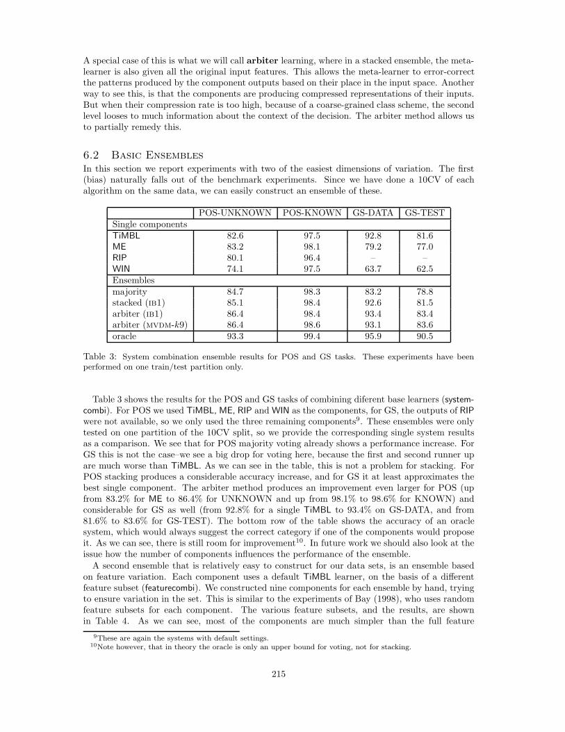
6.2 Basic Ensembles

In this section we report experiments with two of the easiest dimensions of variation. The first(bias) naturally falls out of the benchmark experiments. Since we have done a 10CV of eachalgorithm on the same data, we can easily construct an ensemble of these.

POS-UNKNOWN POS-KNOWN GS-DATA GS-TESTSingle componentsTiMBL 82.6 97.5 92.8 81.6ME 83.2 98.1 79.2 77.0RIP 80.1 96.4 – –WIN 74.1 97.5 63.7 62.5Ensemblesmajority 84.7 98.3 83.2 78.8stacked (ib1) 85.1 98.4 92.6 81.5arbiter (ib1) 86.4 98.4 93.4 83.4arbiter (mvdm-k9) 86.4 98.6 93.1 83.6oracle 93.3 99.4 95.9 90.5

Table 3: System combination ensemble results for POS and GS tasks. These experiments have beenperformed on one train/test partition only.

Table 3 shows the results for the POS and GS tasks of combining diferent base learners (system-combi). For POS we used TiMBL, ME, RIP and WIN as the components, for GS, the outputs of RIPwere not available, so we only used the three remaining components9. These ensembles were onlytested on one partition of the 10CV split, so we provide the corresponding single system resultsas a comparison. We see that for POS majority voting already shows a performance increase. ForGS this is not the case–we see a big drop for voting here, because the first and second runner upare much worse than TiMBL. As we can see in the table, this is not a problem for stacking. ForPOS stacking produces a considerable accuracy increase, and for GS it at least approximates thebest single component. The arbiter method produces an improvement even larger for POS (upfrom 83.2% for ME to 86.4% for UNKNOWN and up from 98.1% to 98.6% for KNOWN) andconsiderable for GS as well (from 92.8% for a single TiMBL to 93.4% on GS-DATA, and from81.6% to 83.6% for GS-TEST). The bottom row of the table shows the accuracy of an oraclesystem, which would always suggest the correct category if one of the components would proposeit. As we can see, there is still room for improvement10. In future work we should also look at theissue how the number of components influences the performance of the ensemble.

A second ensemble that is relatively easy to construct for our data sets, is an ensemble basedon feature variation. Each component uses a default TiMBL learner, on the basis of a differentfeature subset (featurecombi). We constructed nine components for each ensemble by hand, tryingto ensure variation in the set. This is similar to the experiments of Bay (1998), who uses randomfeature subsets for each component. The various feature subsets, and the results, are shownin Table 4. As we can see, most of the components are much simpler than the full feature

9These are again the systems with default settings.10Note however, that in theory the oracle is only an upper bound for voting, not for stacking.

215

POS-UNKNOWN GS-TESTSingle components

ddaasssch pppfsss111111111 82.6 1111111 81.6110000000 44.8 0001000 47.0001100000 41.6 0011000 61.1111100000 53.4 0001100 63.0000011100 62.9 1110000 28.6000000011 38.7 0000111 32.1000011111 72.4 0011100 76.3110011100 72.7 0111110 81.7001111100 68.5 0010100 35.0

Ensemblesmajority 81.6 80.6oracle 95.5 95.0stacked (ib1) 84.8 82.5stacked (mvdm-k9) 85.3 82.6arbiter (mvdm-k9) 86.9 82.7stacked+systems (mvdm-k9) 86.6 82.5

Table 4: Feature combination ensemble results for POS-UNKNOWN and GS-TEST. These experimentshave been performed on one train/test partition only. The stacked+systems entry (bottom row) includesall systems from Table 3 and all feature subsets components.

representation, and hence do not perform very well by themselves. Neither does the majority votingensemble perform well. As an illustration of the power of stacking, however, this experiment issufficient. Both stacked and arbiter version produce better results than the systemcombi ensemblefor POS. For GS, the stacked version is better than systemcombi, but, disappointingly, the arbiterversion is not. Finally, if we put the components of systemcombi and featurecombi together, theresults further improve upon both simple stacked ensembles for POS.

7 Evolution Of Modular Ensemble Systems

In Section 6 four dimensions of variation have been identified that can be used to cause variationamong classifiers, and hence possibly improve the performance of an ensemble. Two of thesedimensions (bias and feature set) were shown to be effective on two of our data sets. Ensemblemethods are a very active area of research and these and other variations are shown to work welltime after time (see Dietterich (2000) and the references therein). What is striking however, isthat so far:

• Few attempts have been made to optimize the divergence in an ensemble directly in order toget better performance11. In most research on combined methods, an ensemble is constructedby making a diverse set in some ad-hoc fashion–as we have done–, and then combining thesecomponents (usually by using voting).

• Moreover, the four dimensions of variation have mainly been studied in isolation. This inspite of the fact that a simultaneous variation in bias and output coding and data set andfeature set might have much more far-reaching effects.

In this section we sketch the outline of a method that can exploit all of the above mentioneddimensions of modularization, while at the same time explicitly optimizing the composition ofthe ensemble using Genetic Algorithms. It is a derivative of the method used for feature and

11We are only aware of work in this direction in the Neural Networks field (e.g. Moriarty and Miikkulainen, 1997;Yao, 1999), but have not yet encountered such work in symbolic Machine Learning.

216

parameter optimization in Section 5. We simply encode the whole ensemble as a large vector ofparameters.

A first population of ensembles is generated with random settings for each component, all com-ponents are trained on the same task, a ’stacked’ second level algorithm learns to combine theoutputs of the ensemble, and the combiner’s test score is used as a fitness value. Subsequentgenerations are formed by cross-over and mutation from the fittest ensembles. Using the scoreof the whole ensemble as a fitness measure ensures the selection of good ’team-players’ as con-stituents, even though we have no good understanding how quality (accuracy) and specialization(de-correlation of errors) contribute to the global solution. This should typically lead to auto-matic modularization of the task. As shown in Table 5, in our first experiments, this method hasa higher accuracy than both the best individual system, and the ’hand-designed’ systemcombi andfeaturecombi systems for the GS task. For POS results are better than systemcombi but the same(stacked version) or slightly worse (arbiter version) than featurecombi.

However, these experiments are only starting to scratch the surface of what is possible withthese methods. We hope that additional performance gains can be realized when more dimensionsof variation are included in the optimized ensembles. But, it remains to be seen whether GA’s arean appropriate optimization method for this application.

POS-UNKNOWN GS-TESTSingle components

ddaasssch pppfsss011011011 71.7 0110000 26.0110100110 65.5 1001110 70.0001011111 76.8 1101000 57.3111111001 70.8 0010111 44.9010111111 80.4 0110010 33.0010111100 72.4 0001111 70.2100111111 74.7 0111111 81.5011000010 52.3 1111100 77.9001100010 41.7 1000001 18.8

Ensembleshandmade-featurecombi stacked 85.3 82.6handmade-featurecombi arbiter 86.9 82.7GA-stacked 85.3 83.3GA-arbiter 86.5 84.4GA-feat+param-stacked 85.8 83.4GA-feat+param-arbiter 86.4 84.0

Table 5: GA optimized feature modular ensembles for POS-UNKNOWN and GS-TEST. These exper-iments have been performed on one train/test partition only. Each component uses a default TiMBLlearner, on the basis of a different feature subset. For the feat+param entries (bottom two rows) theGA optimized both the feature subset as well as the TiMBL parameters. The stacked and arbiter systemsall use TiMBL with mvdm-k9 as the second level learner.

8 Conclusions And Future Work

In this paper we have studied various supervised machine learning techniques and compared theirperformance on a set of well-known NLP tasks such as Grapheme to phoneme conversion, Part ofspeech tagging, and Word sense disambiguation. The methods included in the study are: Neuralnetworks, Memory-based learning, Rule induction, Decision trees, Maximum Entropy Modeling,Winnow Perceptrons, Naive Bayes Method, and Support Vector Machines.

We have run the algorithms on the NLP data sets under indentical conditions, and the resultsof these experiments are in line with previously obtained results (Daelemans et al., 1999). In

217

particular, Memory-based learning performs well across our NLP benchmark tasks. However,on particular tasks, there are strong competitors: On WSD, Support Vector Machines show anoutstanding performance. This algorithm, however, still has trouble scaling up to large NLPtasks, and requires future research on more sophisticated task decomposition strategies. On POS,Maximum Entropy modeling is slightly better than Memory-based learning, but this is mitigatedafter tuning TiMBL’s parameters.

Furthermore, we have also shown how important feature and parameter tuning is, and discussedhow it can be done using GA’s or more traditional search methods. Further work is needed,however, to evaluate the full potential of this approach.

The comparisons clearly demonstrate how the techniques perform very differently on the dif-ferent data sets, and how some of them have serious limitations regarding large input space. Wehave thus also investigated ensemble systems, combinations of different classifier systems, andtheir performance on the same NLP benchmark tasks. We have provided arguments and empiri-cal evidence that stacking is superior to voting in ensemble systems. In particular, using stacking,it seems a good idea (if there is enough training data) to always use ensembles rather than thebest single algorithm.

Using stacked and arbiter combination we have been able to build effective ensembles (beatingevery single component system) from natural collections of components, such as divergent featuresets, and different learners participating in a benchmark. In future work, the remaining twodimensions of variation (i.e. data set modularization, and output coding modularization will beinvestigated as well.

We have proposed a new framework for constructing optimized modular ensemble classifiersusing GA’s. The first evaluations are very promising. In future work, we will continue in thisdirection. In particular, we plan to investigate the development of intermediate representationsthat work well for stacking. The research will also include investigations on advanced hardwareand especially, on parallel computing, in order to tackle the notorious scaling problem caused bymemory and time limits when dealing with large NLP data sets.

A strong motivation behind our theoretical and empirical investigations of the integration ofmachine learning approaches to NLP tasks is the improvement that these new methods may offer tospeech and language applications. Some of the biggest problems in speech and language technologydeal with knowledge acquisition, flexible interaction management, and robust speech processing,all areas where the complexity of the task requires adaptive methods that can classify new itemsand new situations into approriate classes efficiently and with sufficient accuracy. The results onmodularity, combination, and evolutionary optimization will thus have important heuristic valuefor systems that learn (Jokinen, 2000).

The research on appropriate representations and combination of different learning methods intoensembles can also support building of hybrid systems that integrate symbolic and stochasticprocessing as well as supervisedly and unsupervisedly learned representations for improved per-formance. Our methodological studies can thus be related to real-world language and speechapplications which serve as reference points against which various solutions can be further evalu-ated and compared.

218

Word AccuracyTiMBL FAMBL C4.5 ME RIP WIN NB NN SVM

accident 87.1 85.2 69.0 87.8 88.8 88.3 – 87.7 90.8amaze 99.7 99.7 99.1 93.1 98.8 99.1 97.2 99.4 99.1band 87.0 86.7 81.7 82.8 85.8 81.4 85.3 83.5 89.9behaviour 95.5 96.3 95.4 96.1 96.7 95.3 93.3 95.7 94.5bet-n 76.9 66.3 70.0 71.3 62.5 70.0 70.0 59.4 75.0bet-v 79.0 78.0 69.0 84.0 77.0 72.0 71.0 84.0 86.0bitter 56.3 55.8 45.8 57.9 52.1 37.4 59.5 50.5 67.4bother 83.4 77.4 72.3 77.7 77.1 77.4 79.1 77.4 84.3brilliant 52.1 51.7 44.8 55.4 52.9 17.3 55.6 47.3 60.4bury 48.2 50.9 34.1 50.9 48.2 37.9 50.3 40.3 51.8calculate 80.0 74.6 75.4 76.8 81.8 74.3 81.4 80.0 79.3consume 62.7 65.5 51.8 67.3 70.9 63.6 64.6 62.7 71.8derive 65.5 59.0 55.5 70.3 65.2 65.9 61.0 63.8 67.2excess 83.8 84.8 83.5 85.5 82.4 85.9 84.5 81.4 85.5float-a 60.0 52.0 74.0 62.0 66.0 70.0 80.0 54.0 72.0float-n 66.7 64.4 47.8 60.0 50.0 46.7 66.7 54.4 72.2float-v 50.0 47.7 36.2 51.2 41.2 44.6 50.0 37.3 52.7generous 43.6 43.0 37.6 51.5 40.6 44.5 52.1 40.3 50.9giant-a 90.3 92.6 92.6 92.6 92.3 92.6 90.0 91.9 91.3giant-n 80.0 77.4 75.8 77.9 80.8 76.3 78.7 76.3 82.9invade 52.5 50.0 37.5 60.0 48.8 41.3 58.8 48.8 62.5knee 78.3 71.1 68.5 74.9 71.7 69.2 71.9 65.8 77.5modest 58.3 59.8 55.6 65.6 64.4 38.5 61.2 57.6 63.4onion 95.0 97.5 80.0 80.0 80.0 82.5 82.5 92.5 95.0promise-n 67.3 67.4 61.3 73.6 72.3 67.4 69.2 72.6 73.2promise-v 89.2 87.3 85.9 87.6 87.3 85.5 88.6 89.4 92.4sack-n 83.3 72.5 65.8 71.7 75.8 58.3 77.5 73.3 83.3sack-v 99.5 98.4 96.3 96.3 96.3 96.8 97.4 96.3 97.9sanction 80.0 72.3 71.8 74.6 76.4 61.8 80.9 72.7 82.7scrap-n 82.5 77.5 62.5 77.5 68.8 77.5 78.8 47.5 87.5scrap-v 87.5 92.5 92.5 85.0 95.0 95.0 92.5 85.0 87.5seize 60.0 61.5 59.7 62.9 55.0 55.3 58.5 58.5 63.2shake 69.6 68.7 62.6 69.1 67.3 62.2 68.2 67.4 76.2shirt 86.4 85.7 87.2 80.2 87.9 84.6 80.2 83.9 89.5slight 91.9 91.2 90.2 89.5 92.2 90.2 90.0 87.8 90.9wooden 97.6 97.3 97.6 95.4 97.8 95.7 97.0 93.5 97.0best one 5 3 1 4 5 3 2 0 19avg. rank 3.9 4.8 7.1 4.3 5.0 6.6 4.6 6.4 2.3

Table 6: Generalization accuracies (10CV) for the WSD task. The bottom two rows summarize the tableby listing how many times an algorithm was the best one, resp. what its average ranking per word is.

219

References

Abney, S. (1996). Statistical methods and linguistics. In Klavans, J. L. and Resnik, P., editors, TheBalancing Act: Combining Symbolic and Statistical Approaches to Language, pages 1–26. MIT Press,Cambridge, MA.

Aha, D. W., Kibler, D., and Albert, M. (1991). Instance-based learning algorithms. Machine Learning,6:37–66.

Baayen, R. H., Piepenbrock, R., and van Rijn, H. (1993). The CELEX lexical data base on CD-ROM.Linguistic Data Consortium, Philadelphia, PA.

Bay, S. (1998). Combining nearest neighbor classifiers through multiple feature subsets. In Proc. 17thIntl. Conf. on Machine Learning, pages 37–45.

Berger, A., Della Pietra, S., and Della Pietra, V. (1996). A maximum entropy approach to natural languageprocessing. Computational Linguistics, 22(1), March 1996.

Blake, C., Keogh, E., and Merz, C. (1998). UCI repository of machine learning databases.

Brill, E. and Wu, J. (1998). Classifier combination for improved lexical disambiguation. In Proceedings ofthe Seventeenth International Conference on Computational Linguistics (COLING-ACL’98), Montreal,Canada, pages 191–195.

Burges, C. (1998). A tutorial on support vector machines for pattern recognition. Data Mining andKnowledge Discovery, 2(2):955–974.

Campbell, C. (2000). Algorithmic approaches to training support vector machines: A survey. In Proceed-ings of ESANN2000, pages 27–36. D-Facto Publications, Belgium.

Carlson, A., Cumby, C., Rosen, J., and Roth, D. (1999). SNoW User’s Guide. Technical Report UIUC-DCS-R-99-210, University of Illinois at Urbana-Champaign.

Cohen, W. (1995). Fast effective rule induction. In Proceedings of the Twelfth International Conferenceon Machine Learning, pages 115–123, Lake Tahoe, California.

Cost, S. and Salzberg, S. (1993). A weighted nearest neighbour algorithm for learning with symbolicfeatures. Machine Learning, 10:57–78.

Cover, T. M. and Hart, P. E. (1967). Nearest neighbor pattern classification. Institute of Electrical andElectronics Engineers Transactions on Information Theory, 13:21–27.

Daelemans, W. (1996). Experience-driven language acquisition and processing. In Van der Avoird, M.and Corsius, C., editors, Proceedings of the CLS Opening Academic Year 1996-1997, pages 83–95. CLS,Tilburg.

Daelemans, W., Van den Bosch, A., and Zavrel, J. (1999). Forgetting exceptions is harmful in languagelearning. Machine Learning, Special issue on Natural Language Learning, 34:11–41.

Daelemans, W., Zavrel, J., van der Sloot, K., and van den Bosch, A. (2000). TiMBL: Tilburg memorybased learner, version 3.0, reference manual, technical report ILK-0001. Technical report, ILK, TilburgUniversity.

Dietterich, T. and Bakiri, G. (1991). Error-correcting output codes: A general method for improvingmulticlass inductive learning programs. In Proc. of the 9th National Conference on Artificial Intelligence(AAAI-91), pages 572–577.

Dietterich, T. G. (2000). Ensemble methods in machine learning. In Kittler, J. and Roli, F., editors,Proc. of the First International Workshop on Multiple Classifier Systems (MCS 2000), volume 1857 ofLecture Notes in Computer Science, pages 1–15. Springer Verlag, Berlin.

Escudero, G., Marquez, L., and Rigau, G. (2000). A comparison between supervised learning algorithmsfor word sense disambiguation. In Proc. of CoNLL-2000. ACL.

Freund, Y. and Schapire, R. (1997). A decision-theoretic generalization of on-line learning and an appli-cation to boosting. Journal of Computer and System Sciences, 55(1):119–139.

Joachims, T. (1999). Making large-scale SVM learning practical. In Scholkopf, B., Burges, C., and Smola,A., editors, Advances in Kernel Methods - Support Vector Learning. MIT-Press.

Johansson, S. (1986). The tagged LOB Corpus: User’s Manual. Norwegian Computing Centre for theHumanities, Bergen, Norway.

John, G., Kohavi, R., and Pfleger, K. (1994). Irrelevant features and the subset selection problem. InProceedings of the Eleventh International Conference on Machine Learning, pages 121–129, San Mateo,CA. Morgan Kaufmann.

Jokinen, K. (2000). Learning Dialogue Systems. In Proceedings of the LREC 2000 Workshop ”From

220

Spoken Dialogue to Full Natural Interactive Dialogue”, pages 13–17.

Kilgarriff, A. and Rosenzweig, J. (2000). Framework and results for english senseval. Computers and theHumanities, special issue on Senseval, 34(1–2).

Kool, A., Zavrel, J., and Daelemans, W. (2000). Simultaneous feature selection and parameter optimizationfor memory-based natural language processing. In submitted.

Littlestone, N. (1988). Learning quickly when irrelevant attributes abound: A new linear thresholdalgorithm. Machine Learning, 2:285–318.

Michie, D., Spiegelhalter, D. J., and Taylor, C. C. (1994). Machine learning, neural and statistical classi-fication. Ellis Horwood, New York.

Mooney, R. J. (1996). Comparative experiments on disambiguating word senses: An illustration of therole of bias in machine learning. In Proceedings of the Conference on Empirical Methods in NaturalLanguage Processing, EMNLP, pages 82–91.

Moreira, M. and Mayoraz, E. (1998). Improved pairwise coupling classification with correcting classifiers.In Proceedings of the 10th European Conference on Machine Learning, pages 160–171.

Moriarty, D. E. and Miikkulainen, R. (1997). Forming neural networks through efficient and adaptivecoevolution. Evolutionary Computation, 5:373–399.

Ng, H. T. and Lee, H. B. (1996). Integrating multiple knowledge sources to disambiguate word sense: Anexemplar-based approach. In Proc. of 34th meeting of the Assiociation for Computational Linguistics.

Prechelt, L. (1998). Early stopping – but when? In Neural Networks: Tricks of the trade, Lecture Notesin Computer Science 1524, Springer Verlag, Heidelberg, pages 55–69.

Quinlan, J. (1993). c4.5: Programs for Machine Learning. Morgan Kaufmann, San Mateo, CA.

Ratnaparkhi, A. (1997). A linear observed time statistical parser based on maximum entropy models.Technical Report cmp-lg/9706014, Computation and Language, http://xxx.lanl.gov/list/cmp-lg/.

Roth, D. (1998). Learning to resolve natural language ambiguities: A unified approach. In Proc. of AAAI.

Roth, D. (2000). Learning in natural language: Theory and algorithmic approaches. In Proc. of CoNLL’00.ACL.

Stanfill, C. and Waltz, D. (1986). Toward memory-based reasoning. Communications of the acm,29(12):1213–1228.

Tjong Kim Sang, E., Daelemans, W., Dejean, H., Koeling, R., Krumolowski, Y., Punyakanok, V., andRoth, D. (2000). Applying system combination to base noun phrase identification. In Proceedings ofCOLING 2000, Saarbrucken, Germany.

Van den Bosch, A. (1997). Learning to pronounce written words: A study in inductive language learning.PhD thesis, Universiteit Maastricht.

Van den Bosch, A. (1999). Instance-family abstraction in memory-based learning. In Proc. of the 16thInternational Conference on Machine Learning (ICML’99), Bled, Slovenia, pages 39–48.

Van Halteren, H., Zavrel, J., and Daelemans, W. (1998). Improving data driven wordclass tagging bysystem combination. In Proceedings of the Seventeenth International Conference on ComputationalLinguistics (COLING-ACL’98), Montreal, Canada, pages 491–497.

Vapnik, V. (1982). Estimation of Dependencies Based on Empirical Data. Nauca, Moskow, 1979, Enlishtranslation: Springer Verlag, New York.

Weiss, S. and Kulikowski, C. (1991). Computer systems that learn. San Mateo, CA: Morgan Kaufmann.

White, A. and Liu, W. (1994). Bias in information-based measures in decision tree induction. MachineLearning, 15(3):321–329.

Wolpert, D. H. (1992). Stacked generalization. Neural Networks.

Yao, X. (1999). Evolving artificial neural networks. Proceedings of the IEEE, 87(9):1423–1447.

Zell, A., Mamier, G., Vogt, M., et al. (1995). SNNS, Stuttgart Neural Network Simulator, User Manual.University of Stuttgart, version 4.1 edition. Technical report 6/95.

221