Embed Size (px)
Citation preview
DIVA-GIS Version 5.2
Manual
September 2005
Robert J. Hijmans, Luigi Guarino, Andy Jarvis,
Rachel O’Brien, Prem Mathur, Coen Bussink
Mariana Cruz, Israel Barrantes, and Edwin Rojas
ii
Conditions of use
The DIVA-GIS software can be used and distributed freely. The software is provided "as
is", without warranty of any kind, express or implied, including but not limited to the
warranties of merchantability, fitness for a particular purpose and noninfringement. In
no event shall the authors or copyright holders be liable for any claim, damages or
other liability, whether in an action of contract, tort or otherwise, arising from, out of
or in connection with the software or the use or other dealings in the software.
Portions of this computer program are owned by LizardTech, Inc., and are copyright ©
1995-1998, LizardTech, Inc., and/or the University of California. U.S. Patent No.
5,710,835. All rights reserved.
Contributors
DIVA-GIS is currently being developed by Robert J. Hijmans, Luigi Guarino, Andrew
Jarvis, Rachel O’Brien, and Prem Mathur. Edwin Rojas, Mariana Cruz, Coen Bussink,
and Israel Barrantes were involved in the development of earlier versions. Support for
the development has come from the International Plant Genetic Resources Institute
(IPGRI), the UC Berkeley Museum of Vertebrate Zoology, the International Potato
Center (CIP), SINGER/SGRP, FAO, and USDA.
We have benefited from the work of the following persons: M. Sawada (Rook's case),
Gerald Everden and Frank Warmerdam (PROJ4); Andrew Williamson (Shapechk); the
contributors to Delphi Zip Version 1.70
(http://www.geocities.com/SiliconValley/Network/2114/)
DIVA-GIS was improved thanks to bug-reports and/or suggestions made by many
individuals, including Østein Berg, Arthur Chapman, Stefano Diulgheroff, Dirk
Enneking, Tito Franco, Catherine Graham, Stephanie Greene, Lee Hannah, Dave
Hodson, Roel Hoekstra, Andrew Jarvis, Ravish Kumar, Prem Mathur, Andy Nelson,
Andreas Ohr, Xavier Scheldeman, Victor Soto, Jeff White, Louise Willemen, Karen
Williams, and Brian Zutta.
iii
Warning
DIVA-GIS is a relatively new program that is under continuous development and not all
parts have been tested completely. This means that you should never blindly believe
the results of your analysis. Instead, you should always test if DIVA-GIS works well, for
example by manually calculating the expected results for a small number of grid cells.
Or by first doing the calculations with a simple sample data set for which you know the
results.
If you find a possible error, please be so kind to report it!
Please send your comments to [email protected]
Abstract
DIVA-GIS is a free computer program for mapping and for analyzing spatial data. It is
particularly useful for analyzing the distribution of organisms to elucidate geographic
and ecological patterns. It is aimed at persons who cannot afford generic commercial
geographic information system (GIS) software, or do not have the time to learn how to
use these, and for anyone else who wants a GIS tailor-made to analyze biological
distributions. DIVA-GIS supports vector (point, line, polygon) and image and grid data
types. DIVA-GIS can help improve data quality by finding the coordinates of localities
using gazetteers, and by checking existing coordinates using overlays (spatial queries)
of the collection sites and administrative boundary databases. Distribution maps can
then be made. Analytical functions in DIVA-GIS include mapping of richness and
diversity (including based on molecular marker (DNA) data; mapping the distribution of
specific traits; identification of areas with complementary diversity; and analysis of
spatial autocorrelation. DIVA-GIS can also extract climate data for all locations on
land. Ecological niche modeling can be carried out using the BIOCLIM and DOMAIN
algorithms.
iv
Table of Contents
1. INTRODUCTION......................................................... 1
1.1 Conventions used ............................................................... 1 1.2 Installing DIVA-GIS .............................................................. 1 1.3 The DIVA-GIS desktop .......................................................... 2
1.3.1 The Data view ........................................................................2 1.3.2 The Design view ......................................................................5
1.4 File Types and Formats ........................................................ 7 1.4.1 Shapefiles .............................................................................7 1.4.2 Grids ...................................................................................8 1.4.3 Image files ............................................................................8 1.4.4 DBF files ...............................................................................9
1.5 Geographic coordinates ......................................................10
2. THE PROJECT MENU...................................................11
2.1 Projects .........................................................................11 2.2 Import project and Export project..........................................12
3. THE DATA MENU ......................................................13
3.1 Import Points to Shapefile ...................................................14 3.2 Import Text to Line/Polygon.................................................15 3.3 Draw Shape .....................................................................16 3.4 Polygon to Grid.................................................................16 3.5 Points to Convex Polygon.....................................................17 3.6 Selection to new shapefile ...................................................17 3.7 Extract Values by Points......................................................17 3.8 Climate ..........................................................................17 3.9 Assign coordinates .............................................................18 3.10 Check coordinates .............................................................21 3.11 Export gridfile..................................................................23 3.12 Import to gridfile ..............................................................24 3.13 File manager....................................................................24 3.14 Download........................................................................24
4. THE LAYER MENU .....................................................25
4.1 Add layer and Remove layer .................................................26 4.2 Properties .......................................................................26 4.3 Identify ..........................................................................27 4.4 Table.............................................................................27 4.5 Select records ..................................................................27 4.6 Copy and Paste.................................................................28
v
5. THE MAP MENU .......................................................29
5.1 Map to image ...................................................................29
6. THE ANALYSIS MENU ..................................................30
6.1 Point to grid ....................................................................30 6.1.1 Defining Grids ...................................................................... 31 6.1.2 Using the parameters of an existing grid....................................... 33
6.2 Output variables ...............................................................33 6.2.1 Richness ............................................................................. 33 6.2.2 Estimators of Richness ............................................................ 35 6.2.3 Turnover............................................................................. 38 6.2.4 Diversity indices.................................................................... 39 6.2.5 Molecular marker data ............................................................ 39 6.2.6 Reserve selection .................................................................. 41
6.3 Methods of converting point data to grid data ...........................44 6.3.1 Circular neighborhood............................................................. 44
6.4 Point to polygon ...............................................................45 6.5 Point to point...................................................................46 6.6 Summarize Points..............................................................47 6.7 Distance .........................................................................47 6.8 Spatial autocorrelation .......................................................47
6.8.1 Points ................................................................................ 48 6.8.2 Grid .................................................................................. 49
6.9 Histogram .......................................................................49 6.10 Regression ......................................................................49 6.11 Multiple Regression............................................................49
7. THE MODELING MENU .................................................50
7.1 Bioclim / Domain ..............................................................50 7.1.1 Input ................................................................................. 50 7.1.2 Frequency ........................................................................... 51 7.1.3 Outliers .............................................................................. 51 7.1.4 Histogram ........................................................................... 51 7.1.5 Envelope............................................................................. 51 7.1.6 Predict ............................................................................... 52
7.2 External Models ................................................................54 7.3 Evaluation.......................................................................54
7.3.1 Prepare points...................................................................... 54 7.3.2 Create evaluation file ............................................................. 55 7.3.3 Show ROC / Kappa ................................................................. 55
7.4 EcoCrop .........................................................................55 7.5 Terrain Modeling...............................................................58
8. THE GRID MENU.......................................................59
8.1 Describe .........................................................................59 8.2 Overlay ..........................................................................60 8.3 Scalar ............................................................................60
vi
8.4 Reclass...........................................................................60 8.5 Neighbourhood .................................................................61 8.6 Calculate ........................................................................61 8.7 Aggregate .......................................................................62 8.8 Disaggregate....................................................................63 8.9 Cut ...............................................................................63 8.10 Concatenate ....................................................................63 8.11 New ..............................................................................64 8.12 Transect.........................................................................64 8.13 Area..............................................................................64
9. THE STACK MENU .....................................................65
9.1 Make stack ......................................................................65 9.2 Plot...............................................................................66 9.3 Calculate ........................................................................66 9.4 Regression ......................................................................66 9.5 Cluster...........................................................................66 9.6 Export to textfile ..............................................................67
10. THE TOOLS MENU .....................................................68
10.1 Projection.......................................................................68 10.2 Graticule ........................................................................69 10.3 Shift shape......................................................................69 10.4 Georeference image ..........................................................69 10.5 Geo-calculator .................................................................70 10.6 General options ................................................................71
REFERENCES ....................................................................72
DIVA-GIS 5
1
1. INTRODUCTION
This manual explains how to use DIVA-GIS. Additional information, including an
introductory tutorial, exercises, and examples of the use of DIVA-GIS can be found on
the DIVA-GIS website (http://www.diva-gis.org).
1.1 Conventions used
The following conventions are used in this manual:
Italics are used to refer to menus and sub-menus and buttons. A slash (/) is used to
relate a submenu to a menu.
“Quotes” are used to refer to buttons.
Courier font is used for file and directory names and for special keys such as Shift;
File types are referred to by their extension. For example, a dBase file, like data.dbf,
is referred to as a DBF file
1.2 Installing DIVA-GIS
If you downloaded DIVA from the Internet, you need to unzip the downloaded files
first (use e.g. pkzip; www.pkware.com). Then you should click on setup.exe to install
DIVA; also click on this file if you are installing from a CD-ROM. You will be asked in
what directory (folder) you want to install the program. As you can install the
program in any directory you like, in this manual we will refer to this directory as the
<DIVA dir>. By default, DIVA will be installed in the C:\program files\DIVA-GIS\
directory.
DIVA-GIS 5
2
1.3 The DIVA-GIS desktop
The DIVA-GIS window consists of two overlapping parts, which we call views. The Data
view is where you will do most of your work. The Design view is used to produce a
graphical representation of the results of your work that can be saved as a graphics
file, and printed or used in another application.
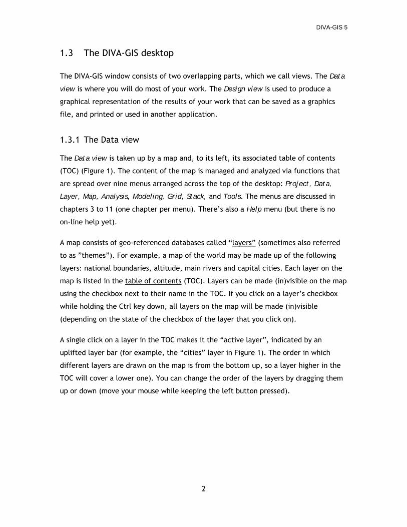
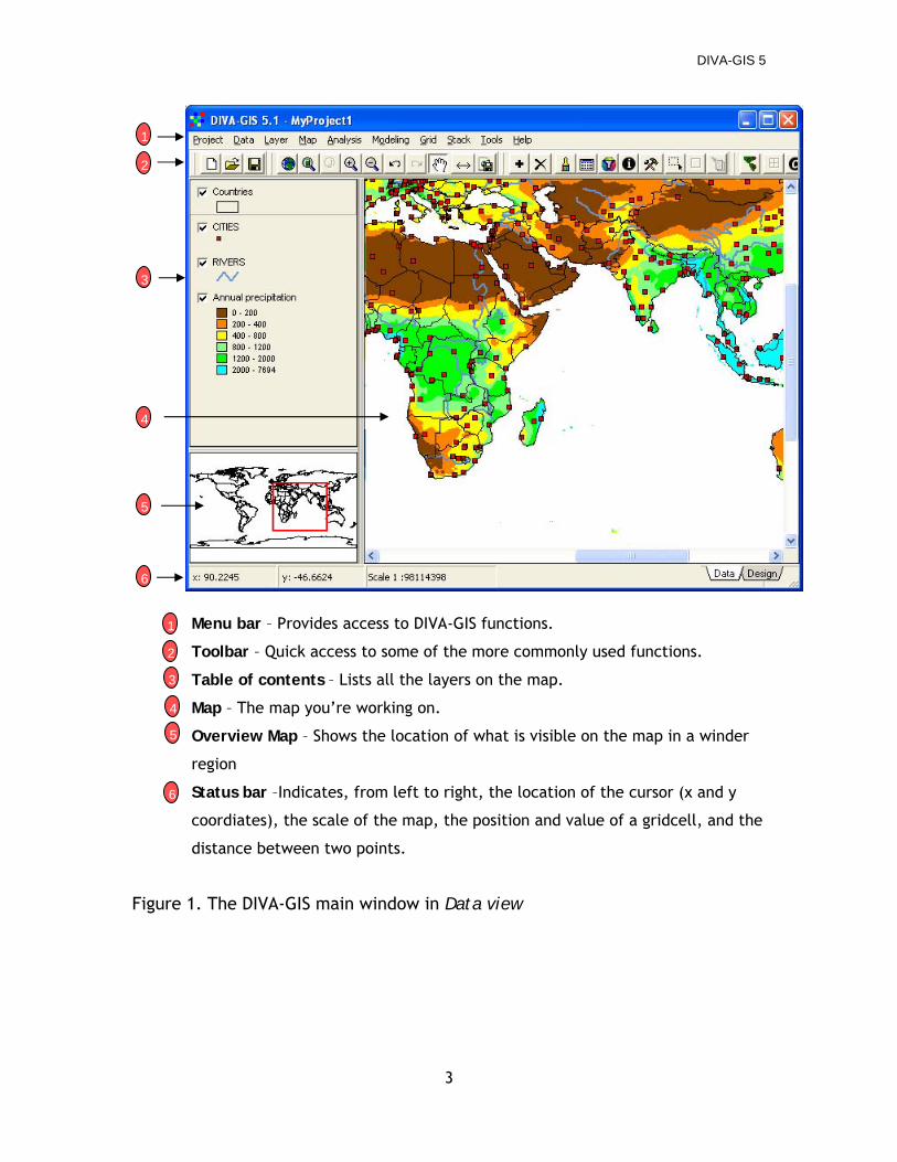
1.3.1 The Data view
The Data view is taken up by a map and, to its left, its associated table of contents
(TOC) (Figure 1). The content of the map is managed and analyzed via functions that
are spread over nine menus arranged across the top of the desktop: Project, Data,
Layer, Map, Analysis, Modeling, Grid, Stack, and Tools. The menus are discussed in
chapters 3 to 11 (one chapter per menu). There’s also a Help menu (but there is no
on-line help yet).
A map consists of geo-referenced databases called “layers” (sometimes also referred
to as ”themes”). For example, a map of the world may be made up of the following
layers: national boundaries, altitude, main rivers and capital cities. Each layer on the
map is listed in the table of contents (TOC). Layers can be made (in)visible on the map
using the checkbox next to their name in the TOC. If you click on a layer’s checkbox
while holding the Ctrl key down, all layers on the map will be made (in)visible
(depending on the state of the checkbox of the layer that you click on).
A single click on a layer in the TOC makes it the “active layer”, indicated by an
uplifted layer bar (for example, the “cities” layer in Figure 1). The order in which
different layers are drawn on the map is from the bottom up, so a layer higher in the
TOC will cover a lower one). You can change the order of the layers by dragging them
up or down (move your mouse while keeping the left button pressed).
DIVA-GIS 5
3
Menu bar – Provides access to DIVA-GIS functions.
Toolbar – Quick access to some of the more commonly used functions.
Table of contents – Lists all the layers on the map.
Map – The map you’re working on.
Overview Map – Shows the location of what is visible on the map in a winder
region
Status bar –Indicates, from left to right, the location of the cursor (x and y
coordiates), the scale of the map, the position and value of a gridcell, and the
distance between two points.
Figure 1. The DIVA-GIS main window in Data view
1
2
3
5
1
2
3
4
6
4
5
6
DIVA-GIS 5
4
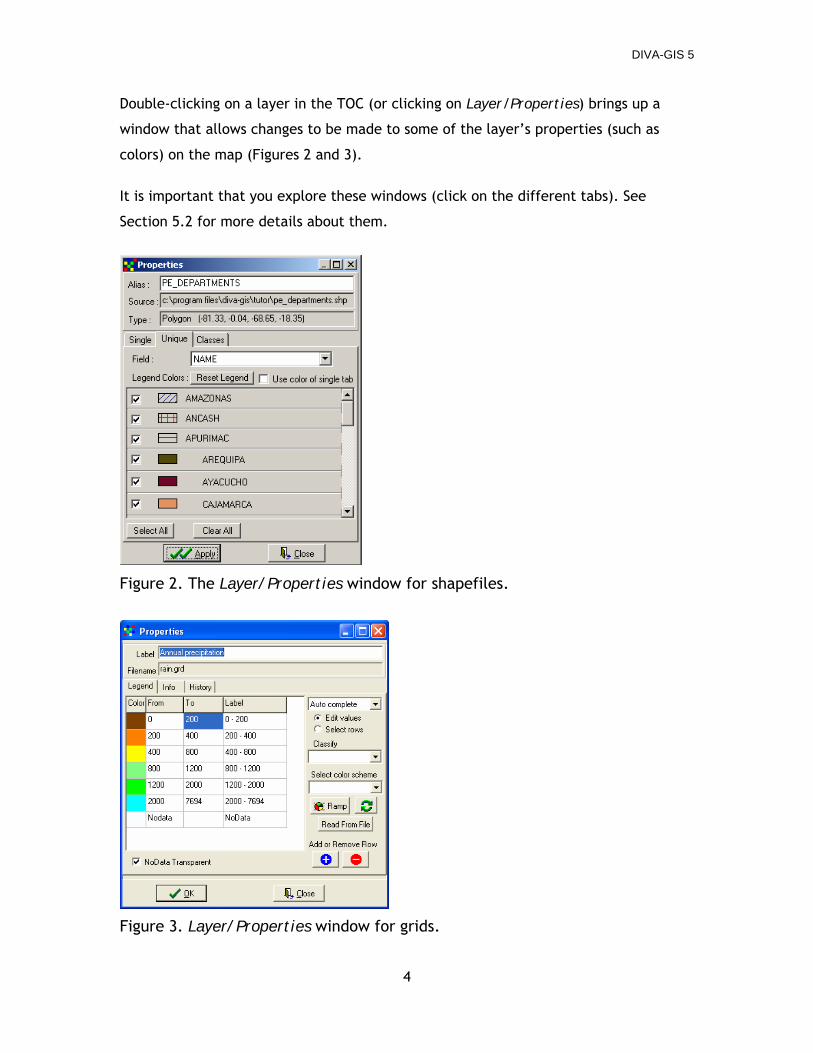
Double-clicking on a layer in the TOC (or clicking on Layer/Properties) brings up a
window that allows changes to be made to some of the layer’s properties (such as
colors) on the map (Figures 2 and 3).
It is important that you explore these windows (click on the different tabs). See
Section 5.2 for more details about them.
Figure 2. The Layer/Properties window for shapefiles.
Figure 3. Layer/Properties window for grids.
DIVA-GIS 5
5
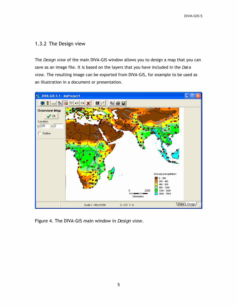
1.3.2 The Design view
The Design view of the main DIVA-GIS window allows you to design a map that you can
save as an image file. It is based on the layers that you have included in the Data
view. The resulting image can be exported from DIVA-GIS, for example to be used as
an illustration in a document or presentation.
Figure 4. The DIVA-GIS main window in Design view.
DIVA-GIS 5
6
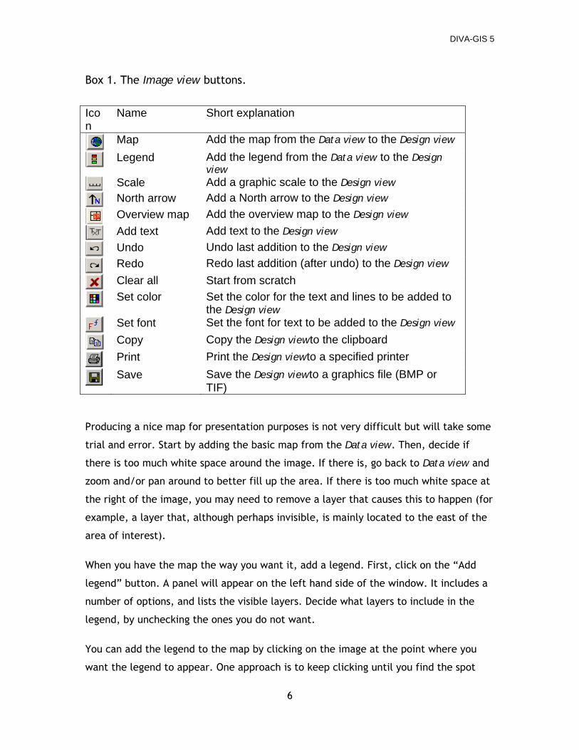
Box 1. The Image view buttons.
Icon
Name Short explanation
Map Add the map from the Data view to the Design view
Legend Add the legend from the Data view to the Design view
Scale Add a graphic scale to the Design view
North arrow Add a North arrow to the Design view
Overview map Add the overview map to the Design view
Add text Add text to the Design view
Undo Undo last addition to the Design view
Redo Redo last addition (after undo) to the Design view
Clear all Start from scratch
Set color Set the color for the text and lines to be added to the Design view
Set font Set the font for text to be added to the Design view
Copy Copy the Design viewto the clipboard
Print Print the Design viewto a specified printer
Save Save the Design viewto a graphics file (BMP or
TIF) Producing a nice map for presentation purposes is not very difficult but will take some
trial and error. Start by adding the basic map from the Data view. Then, decide if
there is too much white space around the image. If there is, go back to Data view and
zoom and/or pan around to better fill up the area. If there is too much white space at
the right of the image, you may need to remove a layer that causes this to happen (for
example, a layer that, although perhaps invisible, is mainly located to the east of the
area of interest).
When you have the map the way you want it, add a legend. First, click on the “Add
legend” button. A panel will appear on the left hand side of the window. It includes a
number of options, and lists the visible layers. Decide what layers to include in the
legend, by unchecking the ones you do not want.
You can add the legend to the map by clicking on the image at the point where you
want the legend to appear. One approach is to keep clicking until you find the spot
DIVA-GIS 5
7
you like; then press “Remove All”, followed by “Add Map”, then the “Add legend”
button and finally OK. The legend will be put where you last had it, because the
coordinates were saved in the text boxes. You can also change these values before you
press OK. Another approach is to add a legend and use the Undo button if you do not
like the place it gets, and try again.
The width of the Table of Contents in the Data view determines its width in the Image
view. Thus, if it is too wide or narrow, go back to the Data view, change it, and try
again in the Image view.
Adding a scale, North arrow, and text to the image follows the same principles.
You can set the color and font for any text that you add to the image. To set the font
for the Table of Contents, however, you must go to the Tools/ Options/Layer menu in
the Data view, change the default font, Close the project and then Open it again.
To export your map from DIVA-GIS, you can print it, copy it to the clipboard (and
paste it into another application), or save it to a graphics file, in bitmap (BMP) or TIF
format.
1.4 File Types and Formats
DIVA uses files of various types and formats. The most important are the shapefile,
gridfile and image file formats for spatial databases and the dBaseIV (DBF) format for
reading and writing external (non spatial) databases.
1.4.1 Shapefiles
Shapefiles are so-called vector databases, describing the location of points (e.g.,
collecting locations), polylines (e.g., roads) or areas (or polygons, e.g., soil types,
countries). A shapefile actually consists of three separate files with the same name
but with different extensions (SHP, SHX and DBF), but they are treated as one file.
There are some shapefiles with additional files (extensions SBN and SBX), but these
are not essential and are not used in DIVA-GIS. The shapefile format was developed by
ESRI, a leading GIS software company. They were initially developed for use in
DIVA-GIS 5
8
ArcView, but now nearly all GIS programs can either directly use them, or import
them.
1.4.2 Grids
Grids are central to the analytical capabilities of DIVA-GIS. A grid divides (a part of)
the world into equal-sized cells. The advantage of using grids as opposed to areas such
as countries or other administrative units is that grid cells of the same size and shape
allow a more objective comparison.
For grid databases, in which an area is divided into equally sized rectangles, DIVA-GIS
gridfiles are used. A gridfile consists of two separate files *.GRI and *.GRD, but DIVA-
GIS treats them as if they were one file. The *.GRI file has the actual data, and the
*.GRD file has metadata and a number of parameters that are needed to read the
*.GRI file properly.
From these two files, DIVA-GIS creates two more files, *.BMP and *.BPW. These files
are derived from the *.GRI and *.GRD files and used to visualize the data on the map,
but are otherwise not essential. If the BMP and BPW are absent, DIVA-GIS creates
these files automatically when opening a gridfile.
The BMP and BPW files can also be used to visualize gridfiles in ArcView and in
ArcExplorer (as images). Unlike in DIVA-GIS, however, the underlying grid data are not
accessible in these programs, and their legend categories cannot be changed. If you
want to use the grid data in another program, you should export them to a suitable
format (Chapter 3).
1.4.3 Image files
Image files are special kinds of grids that can be displayed but not used for analysis, as
the data associated with the different colours in the file are not accessible. A typical
example of such a file would be an air photo or satellite image. DIVA-GIS supports
three image formats: TIFF, JPEG, and mrSID.
DIVA-GIS 5
9
1.4.4 DBF files
DBF (version IV) is a commonly used database format. DIVA-GIS uses it to import and
export tabular data. You can create a DBF file by exporting it from a database
program such as Access, or from a spreadsheet program such as Excel.
If you use Excel, you must take care not to lose data, particularly not to lose precision
(decimals) of the coordinate data, or to create a DBF file with unsupported
characteristics.
The field names (variable names) should be in the first row, and only there. Each
column with data should have a field name. The names of fields may not be repeated,
may not start with a number, and should only consist of letters and numbers. Field
names should not contain characters such as * ^ % ? / - >. Field names have a
maximum length of 11 characters.
In Excel, do not add columns to the right or rows at the bottom of an existing DBF
table. These will not be saved. Instead, use Insert to add columns or rows. You should
NEVER insert or delete rows to a DBF which is part of a shapefile. However, it is fine
to add or delete columns, or to change their content.
To avoid losing decimal places, select the column and set the number of decimals to 5
(or any desired number) using Format/Cells. For numeric fields, there must be a
number in the first cell (i.e. in the second row). Otherwise, the field will be saved as
text. Make these changes before you save the file as DBF (version 4). Always save the
file in the native Excel format (XLS) first, so that you do not lose your data should they
not be saved correctly as DBF.
A common problem is that fields with numbers are saved as text fields. It does not
help to use Format/Cells/Numeric in Excel. That will not change the format to
numeric. Instead, you should do something like insert a new column and multiply the
values in the text column by the numeral 1.0. That transforms the text values to
numeric values (when possible).
DIVA-GIS 5
10
1.5 Geographic coordinates
There are several ways to describe a location on earth. The most commonly used are
degrees of longitude and latitude. A location on earth can be between 180°West and
180°East, and between 90° North and 90° South. Degrees are often subdivided using a
sexagesimal system (a calculus system with 60 as the basic number) of ‘minutes’ and
‘seconds’ (exactly as done with subdivision of hours). For example, a latitude can be
described as e.g., 12°34’15” S (12 degrees, 34 minutes, 15 seconds, Southern
hemisphere).
This system worked fine in the days of paper maps, but it is not very suitable for the
digital age. A decimal system is universally used in geographic computing. In the
decimal system, latitude and longitude are described by a single number each, and no
letters, with the sign indicating the hemisphere (+ = N or E, – = S or W) (e.g., –
12.57083). To convert longitude and latitude in degrees, minutes and seconds to
decimal degrees, the following formula is used:
⎟⎠⎞
⎜⎝⎛ ++⋅=
360060smdhDC
Where DC is the decimal coordinate; d is the degrees (º), m the minutes (’), and s the
seconds (’’) of the sexagesimal system. h = 1 for the northern and eastern hemispheres
and -1 for the southern and western hemispheres. For example, 30º30’0’’ S = -30.500
and 30º15’55’’ N = 30.265. You can do these calculations in a spreadsheet program or
in DIVA-GIS using Tools/Geo-calculator (Chapter 10).
Decimal degrees should normally be recorded with 4 or 5 decimals. At the equator,
one unit of the fourth decimal (0.0001 degrees) equals about 10 meters (less at other
latitudes; not affected by longitude). That should be precise enough for most
applications. If you are using high-precision GPS (with differential correction), 5
decimal places would be warranted. See Wieczoreck et al. (2004) for a thorough
discussion of coordinate precision and uncertainty.
DIVA-GIS 5
11
2. THE PROJECT MENU
The Project menu contains functions for the management of DIVA-GIS project files,
and some related tasks (Box 1).
Box 2. The Project menu.
Icon Sect. Name Short explanation 2.1 New
Starts a new project (map and associated image)
2.1 Open Opens an existing project (file with .DIV extension)
2.1 Close
Closes the current project
2.1 Save
Saves the current project
2.1 Save As
Saves the current project with a new name
2.2 Export Project Exports a project (including all data) to a DIVA-GIS
export file (file with extension “DIX”)
2.2 Import Project
Imports a DIVA-GIS export file (DIX)
2.1 -
A list of the 10 last used DIVA-GIS projects may be found here
Exit
Closes the project and leaves DIVA-GIS
2.1 Projects
A DIVA-GIS project is a description of a DIVA-GIS map: it includes a collection of layers
and their display properties, as well as some general parameters describing the map’s
scale and center. A project file can be closed, saved with a new name, and opened
again using commands from the Project menu. To create a new project, select New.
This creates an empty map that can be filled by adding features using Layer/Add. You
can save a project by clicking on Save. Project files have the extension DIV. The names
of the last 10 projects you saved are listed at the bottom of the Project menu to allow
quick access to these files. You can open a recently used project by selecting it from
this list.
DIVA-GIS 5
12
It is important that you clearly understand the difference between a DIVA-GIS project
file (DIV) and the layers (files) that make up the map. The project file does not
contain the actual data, it only points to the files containing the data pertaining to the
different layers included in the project, and stores map properties (such as scale).
Relative paths (e.g., \diva\myshp.shp) are stored for data files that, in the folder
structure, are below the project file. This allows for sharing projects over a network,
or saving them on a CD-ROM (different drive letters can be used). For all other files,
the absolute path is stored (e.g. c:\mydata\diva\myshp.shp). It is also possible to use
network paths (e.g., \\network\share\shape.shp).
This means that if you delete a project file, all your data will be still be available.
However, if you delete, or rename, a data file, a project file will not be able to find it
anymore, and DIVA-GIS will show a message indicating this.
2.2 Import project and Export project
Another way to share a DIVA-GIS project is to place all its contents into a DIVA-GIS
export file (extension DIX). In contrast to a DIV file, the DIVA-GIS export file contains
the project file and all the layers (data files). You can send such an export file to
another DIVA-GIS user, who can then import it into DIVA, or you can use it to simply
store all files pertaining to a project in one location. These files are compressed, and
they do not take up much disk space; they can often be sent to another user via email.
To import a project file, you must indicate where the data should be expanded, and
under which project name. Typically, you would make a new directory for this, so that
it is clear which files belong to a specific project that you imported.
DIVA-GIS 5
13
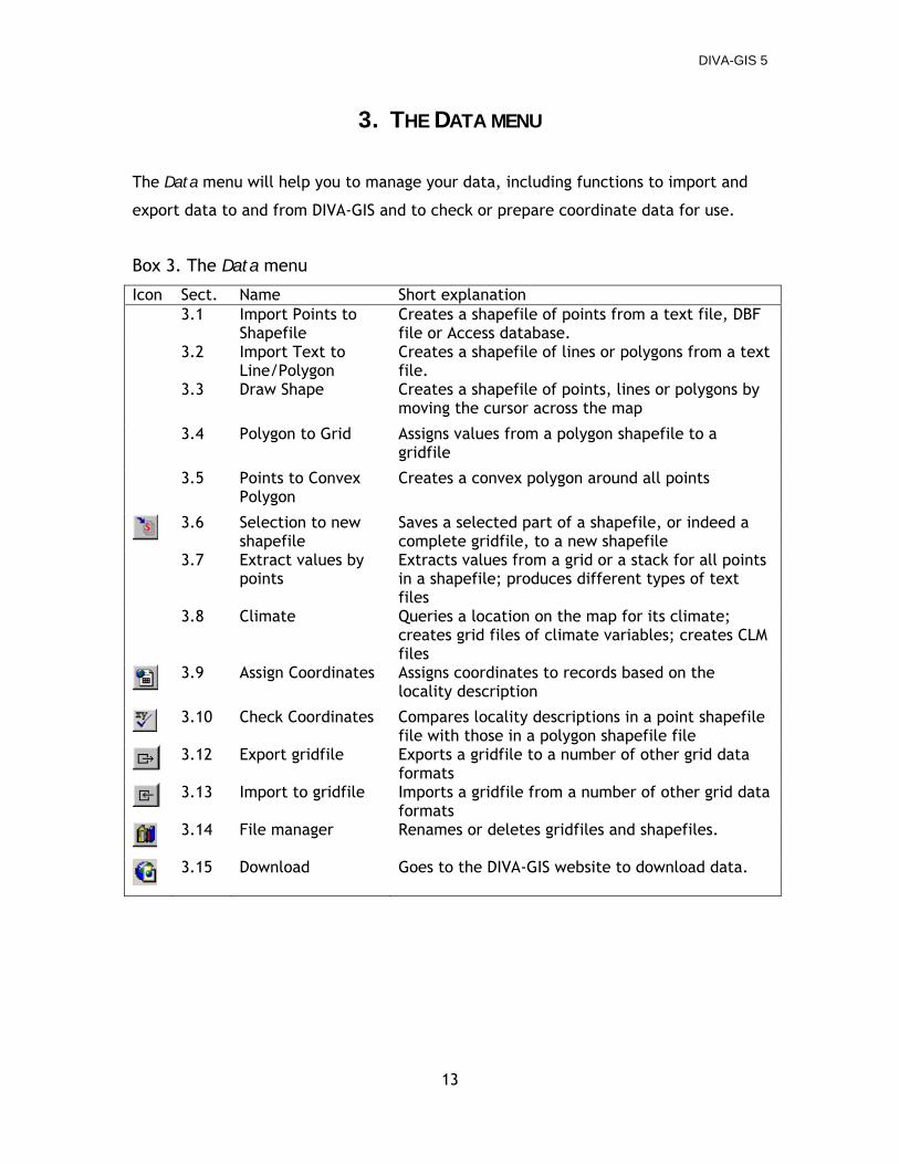
3. THE DATA MENU
The Data menu will help you to manage your data, including functions to import and
export data to and from DIVA-GIS and to check or prepare coordinate data for use.
Box 3. The Data menu
Icon Sect. Name Short explanation 3.1 Import Points to
Shapefile Creates a shapefile of points from a text file, DBF file or Access database.
3.2 Import Text to Line/Polygon
Creates a shapefile of lines or polygons from a text file.
3.3 Draw Shape Creates a shapefile of points, lines or polygons by moving the cursor across the map
3.4 Polygon to Grid Assigns values from a polygon shapefile to a gridfile
3.5 Points to Convex Polygon
Creates a convex polygon around all points
3.6 Selection to new
shapefile Saves a selected part of a shapefile, or indeed a complete gridfile, to a new shapefile
3.7 Extract values by points
Extracts values from a grid or a stack for all points in a shapefile; produces different types of text files
3.8 Climate Queries a location on the map for its climate; creates grid files of climate variables; creates CLM files
3.9 Assign Coordinates Assigns coordinates to records based on the
locality description
3.10 Check Coordinates Compares locality descriptions in a point shapefile file with those in a polygon shapefile file
3.12 Export gridfile Exports a gridfile to a number of other grid data
formats
3.13 Import to gridfile Imports a gridfile from a number of other grid data
formats
3.14 File manager
Renames or deletes gridfiles and shapefiles.
3.15 Download
Goes to the DIVA-GIS website to download data.
DIVA-GIS 5
14
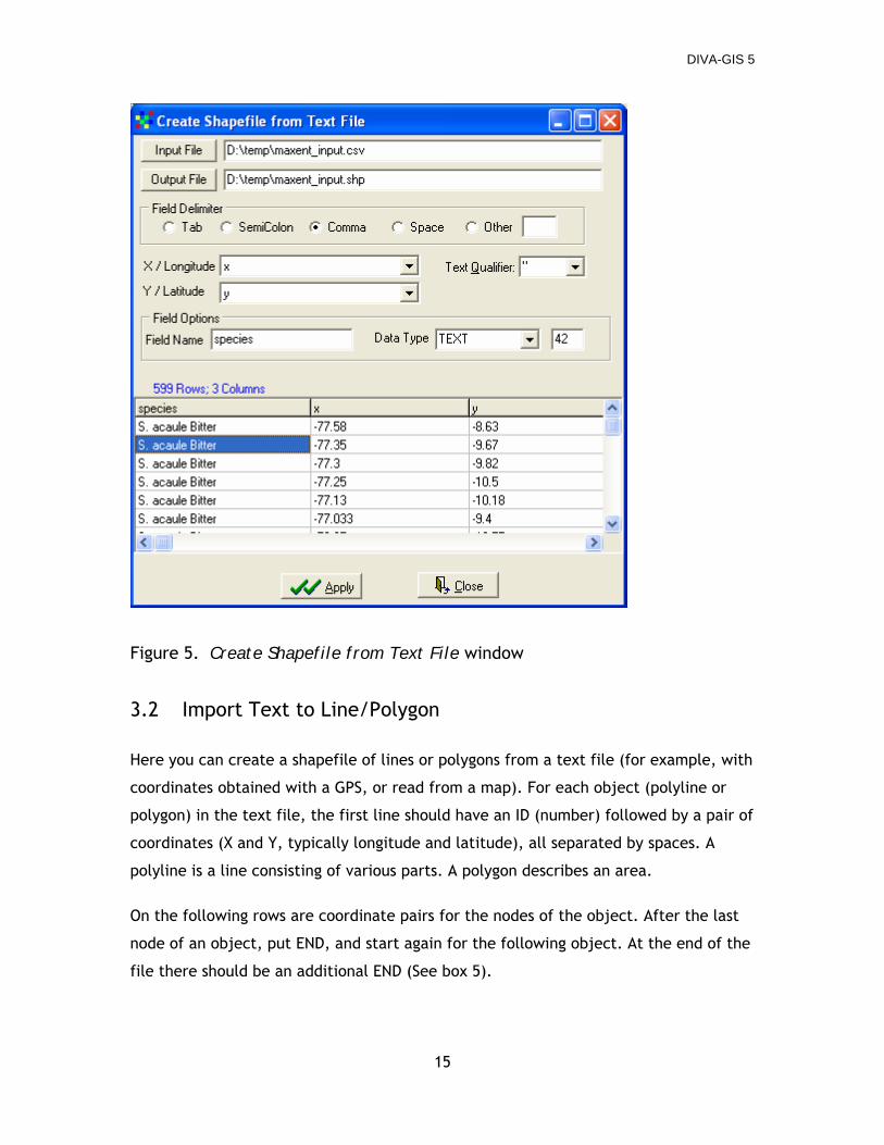
3.1 Import Points to Shapefile
Here you can create a shapefile of points from either a text file, a DBF file, or an
Access database.
The TXT file must have a header row containing the variable names. It does not matter
whether the columns are separated by spaces or a symbol (such as a comma or tab):
the importation wizard will read your data anyway when you tick the appropriate box
specifying the separator (Figure 5). However, ‘tab-separated’ is probably best. Using
commas as separators causes problems when you have a field with locality
descriptions, which may well include commas.
DIVA will figure out for itself what type of data is present in each column of the
database: text, or integer (whole) or real (decimal) numbers; but you may change this
automatically generated setting. The same goes for the maximum number of spaces
that a value of the variable will need. If you indicate fewer spaces than are actually
used, the data will be truncated (cut off at the position that you indicated).
With Import Points to Shapefile/From dBase IV file (DBF) you can make a shapefile of
points from a DBF file if that DBF contains fields with latitude and longitude (both in
decimal degrees). First, you must indicate the filename of your DBF file. And you must
provide an output filename that is different from your input filename.
The program then reads the input file and allows you to select the fields that have the
X (longitude) and Y (latitude) coordinate data. By default, only numerical fields are
listed for you to choose from. However, you can check the “Include Text Fields” box
to see text fields as well. If you use a text field for the X and Y coordinates, DIVA-GIS
will attempt to transform the text values to numbers. Where this is not possible, or
where there is no entry at all, an “empty” record is created. That is, the record is
copied to the DBF table of the shapefile, but no associated point is created.
DIVA-GIS 5
15
Figure 5. Create Shapefile from Text File window
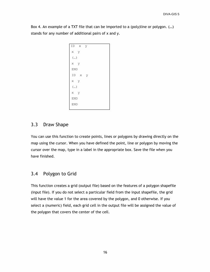
3.2 Import Text to Line/Polygon
Here you can create a shapefile of lines or polygons from a text file (for example, with
coordinates obtained with a GPS, or read from a map). For each object (polyline or
polygon) in the text file, the first line should have an ID (number) followed by a pair of
coordinates (X and Y, typically longitude and latitude), all separated by spaces. A
polyline is a line consisting of various parts. A polygon describes an area.
On the following rows are coordinate pairs for the nodes of the object. After the last
node of an object, put END, and start again for the following object. At the end of the
file there should be an additional END (See box 5).
DIVA-GIS 5
16
Box 4. An example of a TXT file that can be imported to a (poly)line or polygon. (…)
stands for any number of additional pairs of x and y.
3.3 Draw Shape
You can use this function to create points, lines or polygons by drawing directly on the
map using the cursor. When you have defined the point, line or polygon by moving the
cursor over the map, type in a label in the appropriate box. Save the file when you
have finished.
3.4 Polygon to Grid
This function creates a grid (output file) based on the features of a polygon shapefile
(input file). If you do not select a particular field from the input shapefile, the grid
will have the value 1 for the area covered by the polygon, and 0 otherwise. If you
select a (numeric) field, each grid cell in the output file will be assigned the value of
the polygon that covers the center of the cell.
ID x y
x y
(…)
x y
END
ID x y
x y
(…)
x y
END
END
DIVA-GIS 5
17
3.5 Points to Convex Polygon
This creates a "bounding" convex polygon around a set of points. For example, you can
use this to make a “range map” from a set of points representing point localities for a
species. If you want to use all the points in the shapefile, use the “single” tab. If you
want to create more than one range map, use the “Multiple” tab and specify which
field and which values in that field you want to use to distinguish the points that will
be bounded.
3.6 Selection to new shapefile
This saves a selected part of the active (elevated in legend) shapefile to a new
shapefile. Parts of shapefiles can be selected graphically, right on the map, or by
querying the database. The selection procedure is explained in Chapter 5.
3.7 Extract Values by Points
The Extract tool assigns values to the locations specified in a points shapefile. You can
extract values from a polygon shapefile, a gridfile, a stack or a CLM file (see below). In
all cases, the result is a TXT file.
If you extract values from a stack, you can select a field in the point layer that will be
used to "match the grids by class". That means that it will only extract values from a
grid when the attribute of a point (for the selected field) matches the name of the
grid.
3.8 Climate
DIVA-GIS comes with a climate data set for the whole world, excluding major water
bodies (oceans) and Antarctica. These data are available at different spatial
resolutions, and can be downloaded from the DIVA-GIS website. The climate data are
stored in a special format (CLM files) to allow quick access and reduce storage space
requirements. You can also use your own climate data in DIVA-GIS.
DIVA-GIS 5
18
With Climate/Point you can click on the map (on land!) and DIVA-GIS will show climate
data for that location. The window shows the altitude (in meters above sea level) and
monthly average minimum and maximum temperature (°C) and monthly precipitation
(mm), both as tables and graphs. It also shows 19 bioclimatic variables derived from
these monthly data.
Climate/Map provides a tool to map a specified climate variable over a specified area.
When you press the “Read from layer” button in the Climate/Map window, the
dimensions of the active layer will be copied to the minimum and maximum
coordinates. By clicking “Adjust”, the dimensions of the output gridfile are adjusted to
the grid cells of the climate database. You can also draw a rectangle on the map to
define the area (“Draw rectangle” button). Choose the variable that you need and
whether you want a gridfile for the current or for the projected future climate. The
result will be displayed automatically if you check “Add to map”.
In the Climate/Make CLM files window you can construct CLM files from your own
climate grids. CLM files are used to store grids of monthly climate data in DIVA-GIS.
All input files (gridfiles) must have the same number of rows and columns and the
same origin. You must always provide a gridfile with altitude data. If you do not have
such a file, you can replace it with any other file (as long as it has data and nodata on
the right places, and of course, the output altitude file should be discared). It is
important to note that cells with ‘nodata’ in the altitude file will not be stored in the
CLM files.
The output of Make CLM files should always include the files index.clm and a *.cli file,
without which the climate data files cannot be read properly. Store all files in a single
folder. Set the default path for the climate data to that folder (in Tools/General
Options).
3.9 Assign coordinates
The Assign coordinates function can help you to find coordinates for records that only
have a locality description.
DIVA-GIS 5
19
Coordinate data are often absent in biological specimen databases, particularly for
older collections (Greene and Hart, 1996; Wieczorek et al., 2004). However, most
records, even the oldest, are accompanied by a locality description of some kind.
Coordinates can be assigned to such records by searching for the locality names on
maps or in gazetteers. A gazetteer is a list of names of geographic features, with the
coordinates of their locations and other information. Fortunately, there are digital
gazetteers available to make searching easier. DIVA-GIS uses the database of foreign
geographic feature names from the U.S. National Imagery and Mapping Agency's (NIMA)
(http://gnswww.nima.mil/geonames/GNS/index.jsp). You can download these country
gazetteers from the DIVA-GIS website.
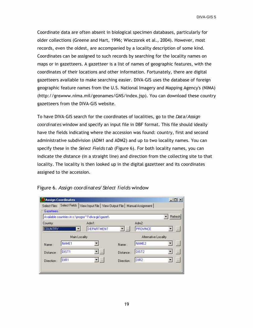
To have DIVA-GIS search for the coordinates of localities, go to the Data/Assign
coordinates window and specify an input file in DBF format. This file should ideally
have the fields indicating where the accession was found: country, first and second
administrative subdivision (ADM1 and ADM2) and up to two locality names. You can
specify these in the Select Fields tab (Figure 6). For both locality names, you can
indicate the distance (in a straight line) and direction from the collecting site to that
locality. The locality is then looked up in the digital gazetteer and its coordinates
assigned to the accession.
Figure 6. Assign coordinates/Select fields window
DIVA-GIS 5
20
Not all fields are obligatory. As a minimum, you must have a field with the name of
the country. This name should be the 3-letter ISO code for the country (e.g. BOL for
Bolivia). If you do not want to use that, you can use another name, but must then
assure that the fieldname and the gazetteer filename are the same, by renaming the
gazetteer file you downloaded (by default, these have been given the ISO county
codes). Your database must also have an ADM1 (first administrative division of the
country), or ADM2 or locality field. Obviously, if you only have ADM1, the coordinate
assignment will be very imprecise.
There are two locality fields because the narrative description of a collecting location
often looks something like “collected in A, 20 km east of B”. In this case, A should be
the first locality and B the second. For the second location (B), the data on distance
(20 km) and direction (east) should be indicated. If, and only if, A is not found, B will
be searched for and, if it is found, the collecting site will be estimated as 20 km east
of B. In other words, the narrative locality description should be summarized in a
number of well defined fields. Distance should be expressed in kilometers. Direction
must be expressed in text, using the codes in Table 1. As distances by road (and not
as the crow flies) are typically reported, you may want to adjust reported distances.
Table 1. Direction codes
Direction Code North N North-northeast NNE Northeast NE East-northeast ENE East E East-southeast ESE Southeast SE South-southeast SSE South S South-southwest SSW Southwest SW West W West-southwest WSW West-northwest WNW Northwest NW North-northwest NNW
DIVA-GIS 5
21
The gazetteer is divided into country files. These files are not all automatically
installed with DIVA-GIS. You can check which files are present by clicking on the
gazetteers list-box on the Data/Assign coordinates window. If the countries you need
are not included, you must locate the files you need on the DIVA-GIS website. The
default location for these files is the <divadir>\gazet folder. You can change this
folder under Tools/General Options.
DIVA-GIS will generate a new output file that contains the input data (such as
COUNTRY and ADM1) and four additional columns: LATITUDE, LONGITUDE, CODE and
COMMENT (Table 2). You can also include any of the other fields in the input database.
You have to go over the comments in the output window carefully to decide which
coordinates you want to accept, which you want to verify, and which you do not want
to use.
Table 2. Possible codes and comments
Code Comment 1 Assigned 2 Assigned to a similar name (San Franzisco ~ San Francisco) 3 n duplicate locality names found (x,y), (x,y), (x,y) 4 Place name (abc) not found (used ADMn = ) 5 Warning: distance from locality name was xxx km (> 50 km) 11 Country (= xxx) not found (no coordinates assigned) 12 ADM1 (= xxx) not found (no coordinates assigned) 13 ADM2 (= xxx) not found (no coordinates assigned) 14 Impossible angle
3.10 Check coordinates
The Check coordinates facility helps you to verify whether coordinates are correct.
The first time you make a shapefile of your database you are most likely to
immediately spot some gross errors. For example, if you have a file of terrestrial bird
specimen from the Solomon Islands, it is likely that some dots will fall in the ocean,
and there might even be one in Siberia. These impossible or unlikely locations are easy
to spot, and often also easy to correct. They may well be just typing errors. However,
it is likely that there will also be other errors that cannot be spotted so easily.
DIVA-GIS 5
22
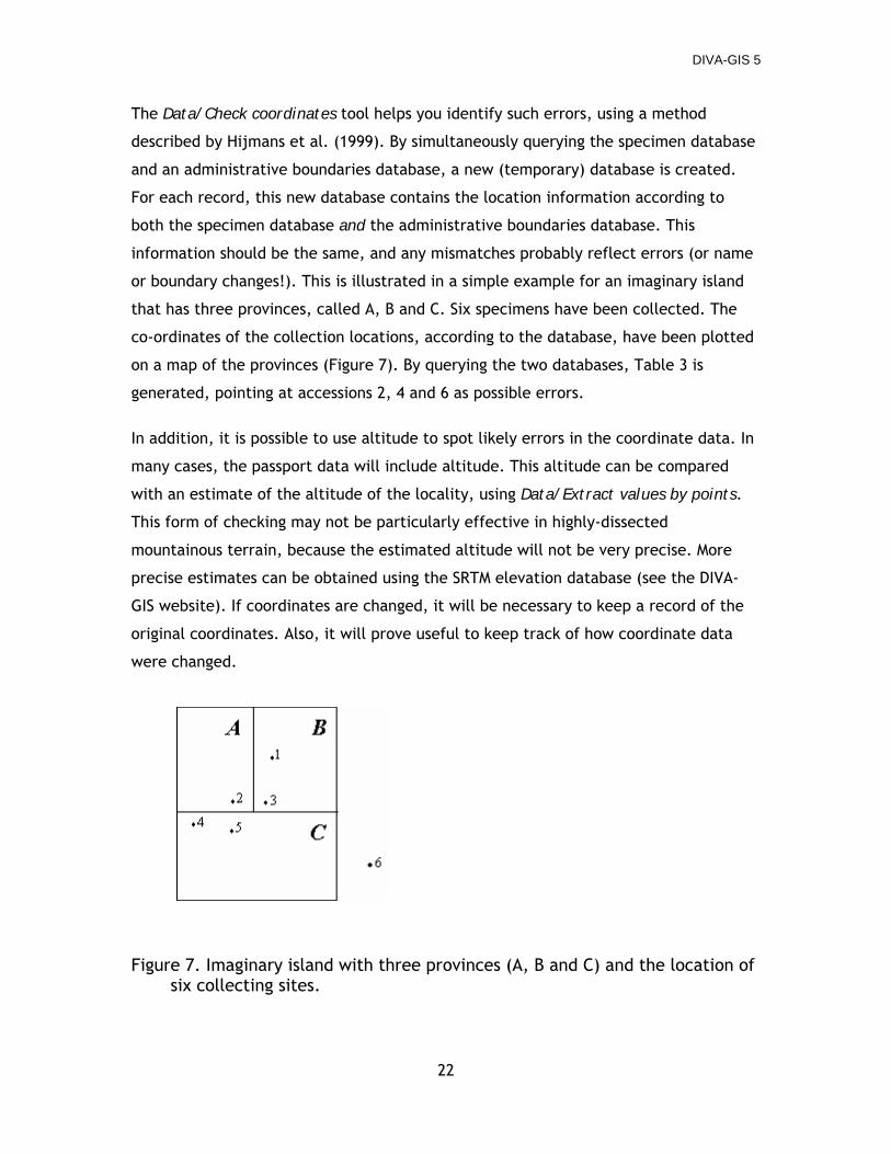
The Data/Check coordinates tool helps you identify such errors, using a method
described by Hijmans et al. (1999). By simultaneously querying the specimen database
and an administrative boundaries database, a new (temporary) database is created.
For each record, this new database contains the location information according to
both the specimen database and the administrative boundaries database. This
information should be the same, and any mismatches probably reflect errors (or name
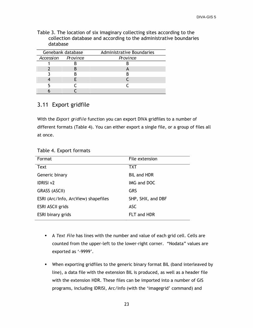
or boundary changes!). This is illustrated in a simple example for an imaginary island
that has three provinces, called A, B and C. Six specimens have been collected. The
co-ordinates of the collection locations, according to the database, have been plotted
on a map of the provinces (Figure 7). By querying the two databases, Table 3 is
generated, pointing at accessions 2, 4 and 6 as possible errors.
In addition, it is possible to use altitude to spot likely errors in the coordinate data. In
many cases, the passport data will include altitude. This altitude can be compared
with an estimate of the altitude of the locality, using Data/Extract values by points.
This form of checking may not be particularly effective in highly-dissected
mountainous terrain, because the estimated altitude will not be very precise. More
precise estimates can be obtained using the SRTM elevation database (see the DIVA-
GIS website). If coordinates are changed, it will be necessary to keep a record of the
original coordinates. Also, it will prove useful to keep track of how coordinate data
were changed.
Figure 7. Imaginary island with three provinces (A, B and C) and the location of six collecting sites.
DIVA-GIS 5
23
Table 3. The location of six imaginary collecting sites according to the collection database and according to the administrative boundaries database
Genebank database Administrative Boundaries Accession Province Province
1 B B 2 B A 3 B B 4 E C 5 C C 6 C
3.11 Export gridfile
With the Export gridfile function you can export DIVA gridfiles to a number of
different formats (Table 4). You can either export a single file, or a group of files all
at once.
Table 4. Export formats
Format File extension
Text TXT
Generic binary BIL and HDR
IDRISI v2 IMG and DOC
GRASS (ASCII) GRS
ESRI (Arc/Info, ArcView) shapefiles SHP, SHX, and DBF
ESRI ASCII grids ASC
ESRI binary grids FLT and HDR
A Text File has lines with the number and value of each grid cell. Cells are
counted from the upper-left to the lower-right corner. “Nodata” values are
exported as ‘-9999’.
When exporting gridfiles to the generic binary format BIL (band interleaved by
line), a data file with the extension BIL is produced, as well as a header file
with the extension HDR. These files can be imported into a number of GIS
programs, including IDRISI, Arc/Info (with the ‘imagegrid’ command) and
DIVA-GIS 5
24
ArcView (where they can be opened as an “image”). If you need a file in the
similar formats BIP or BSQ, you can rename the extension of the output file,
because these are the same when only one grid (or “band”) is stored in a file.
When exporting grids to IDRISI (version 2 and earlier), the result is a data file
with extension IMG and documentation file with extension DOC.
Files in the GRASS (ASCII) format can be imported to GRASS using the command
r.in.ascii.
Grids can also be exported to shapefiles (with rectangular polygons). This can be
particularly useful when you want to use the data in ArcView but do not have the
Spatial Analyst extension that allows visualizing and manipulating grids (or the grid
module in ArcInfo). In other cases, it would be more appropriate to export the gridfile
to an “ASCII grid” or a “floating point” grid (extension FLT and HDR).
3.12 Import to gridfile
With the Import to gridfile module, you can import one or many grid data files into
DIVA-GIS from the IDRISI (IMG or RST), generic binary (BIL/BIP/BSQ), and ESRI binary
export formats.
3.13 File manager
With the File Manager you can delete, copy and rename shapefiles and gridfiles. As
both shapefiles and gridfiles in fact consist of more than one file, this can be a very
helpful utility.
3.14 Download
This launches your Internet browser and the webpage http://www.diva-gis.org/data,
from which you can download geo-referenced databases.
DIVA-GIS 5
25
4. THE LAYER MENU
The Layer menu (Box 5) allows you to add and delete a layer to a project, and change
a layer’s properties. A layer can be either a shapefile, a DIVA-GIS gridfile, or a
georeferenced image (TIF, JPG or SID), but most functions in the Layer menu refer to
shapefiles. Gridfiles and shapefiles for all countries of the world are available from the
DIVA-GIS website.
Box 5. The Layer menu one symbol missing
Icon Sect. Name Short explanation
4.1 Add Layer Adds a layer (theme) to the map
4.1 Remove Layer Removes the active layer from the map
4.2 Properties Changes the style, color, and size of lines of the
active layer
Add labels Adds labels to a layer on the map, using one the
fields in the shapefile database
4.3 Identify Feature Shows the attribute data of a geographic feature of
the active layer after clicking on it
4.4 Table Shows the attribute data of the active layer
(shapefiles only)
Filter Displays a sub-set (e.g. species, country) of the
records from the active layer (shapefiles only)
4.5 Select Records Selects records from the active layer (shapefiles only)
that comply with a specific condition (query).
4.5 Select Features Selects point features by clicking or drawing a
rectangle on the map
4.5 Clear Selection Unselects the currently selected point features of the
active layer.
4.6 Copy Copies the active layer to the clipboard
4.6 Paste Pastes a layer from the clipboard to the map
Hide/Show
Legend Hides or shows information on the active layer in the legend
DIVA-GIS 5
26
4.1 Add layer and Remove layer
Use Layer/Add from the menu bar to add a layer to the map window,. The new layer
is added on top of the list of layers already in the legend. To remove a layer from the
project, click on it once in the legend, to make it the active layer, and then click on
Layer/Remove. This will not delete the data; it will only remove the link to it from the
current project. Multiple layers can be selected, and then removed together, by
clicking on them (in the legend) while holding the down the Shift key.
4.2 Properties
Properties of the spatial objects of a shapefile, such as the size and shape of points
and the colour of polygons, can be modified using Layer/Symbol. You should first
make it the active layer by clicking on it in the legend. Double-clicking on a layer in
the legend also activates the Properties window. There are three ways to change the
symbols:
1. you can change them all at once (use the Single tab)
2. you can give every unique element a different symbol according to one of
its attributes (Unique) or
3. you can classify the numeric attributes and give a different symbol to
each class.
Use the reset button every time you choose a different attribute or number of classes.
Tip: if you want all polygons transparent except for one , you should first make the
polygons transparent in the Single tab and then go to Unique to change the only
polygon you want with a solid fill.
DIVA-GIS 5
27
4.3 Identify
On selecting Identify, a window will appear when you click on the map. When you
click on an item (geographic feature) on the map’s active layer, the Identify window
shows the records of the database and their values for that item. If you click on more
than one item, e.g., a number of points with (nearly) the same location, the data for
all these items are made available. The number of the visible record and the total
number of records are indicated on top of the list of variables (e.g., “Rec 1 of 5”). The
“up” and “down” buttons (arrows) on the right of the list can be used to toggle
between the selected records. If the active layer is a gridfile, the column, row and
value of the grid cell that was clicked on are shown.
4.4 Table
Table allows you to view the database of the active layer (shapefile). If you click on a
record in the table, the location of the corresponding geographic objectwill be
highlighted. You can also move the center of the map to that object.
4.5 Select records
Records can be selected for various purposes. For example, to save a subset of a layer
to a new file, or to find geographic features that meet particular conditions. The
selected items will be displayed in a different color (yellow is the default). You can
make a selection by either making a query in the Select Records window, or by
drawing on the map after clicking on the Select Features button. Only layers that are
made from shapefiles can be selected from.
In the Select Records window you can either select by values, or by query. The first
option is useful for variables with a limited number of values, which are typically non-
numerical. Select the variable and all values will be listed. Then select the values to
include in the selection. When using a query, you must select a variable, a criterion
and the value. Use the ‘Add’ button puts the query in the dialog box, and continue
DIVA-GIS 5
28
adding additional conditions using “AND”, “OR” or condition parentheses. When you
are ready, click ‘Apply’.
Selections can also be made using Select features, by clicking on a map item or
drawing an area (click, keep your finger down, and move the mouse). The shape of
the selection window (rectangle, circle, etc.) can be set in Tools/General options.
Selections can be cleared using Clear selection. The selection can also be converted to
(saved as) a new shapefile with Data/Selection to new shapefile.
4.6 Copy and Paste
The Copy and Paste functions can be used to copy and paste a layer in the legend. This
is useful if you want to use one layer more than once on the same map. For example,
a layer of a country can be used as the lowest layer, to give a background color, and –
this time with transparent polygons – as the highest layer to place departmental
boundaries on top of all other layers.
DIVA-GIS 5
29
5. THE MAP MENU
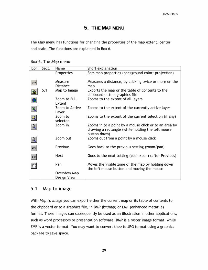
The Map menu has functions for changing the properties of the map extent, center
and scale. The functions are explained in Box 6.
Box 6. The Map menu
Icon Sect. Name Short explanation Properties Sets map properties (background color; projection)
Measure
Distance Measures a distance, by clicking twice or more on the map.
5.1 Map to Image
Exports the map or the table of contents to the clipboard or to a graphics file
Zoom to Full
Extent Zooms to the extent of all layers
Zoom to Active
Layer Zooms to the extent of the currently active layer
Zoom to
selected Zooms to the extent of the current selection (if any)
Zoom in Zooms in to a point by a mouse click or to an area by
drawing a rectangle (while holding the left mouse button down)
Zoom out Zooms out from a point by a mouse click
Previous Goes back to the previous setting (zoom/pan)
Next Goes to the next setting (zoom/pan) (after Previous)
Pan Moves the visible zone of the map by holding down
the left mouse button and moving the mouse Overview Map Design View
5.1 Map to image
With Map to Image you can export either the current map or its table of contents to
the clipboard or to a graphics file, in BMP (bitmap) or EMF (enhanced metafile)
format. These images can subsequently be used as an illustration in other applications,
such as word processors or presentation software. BMP is a raster image format, while
EMF is a vector format. You may want to convert thee to JPG format using a graphics
package to save space.
DIVA-GIS 5
30
6. THE ANALYSIS MENU
This chapter describes the methods for analyzing biological distribution data available
in DIVA-GIS. These analyses are all based on the location (latitude and longitude) and
additional attributes of point data. The points represent locations where a specimen
was collected, or where any observation of the presence of a specific biological unit
(e.g., species, landrace, genotype, allele) was made. These points should be in the
active (shapefile) layer in the DIVA-GIS project (a shapefile is made active by adding it
to the map and clicking on its legend entry once, which highlights it). The output of
the analysis routines can be a gridfile, a shapefile, or a database file (DBF).
Box 7. The Analysis menu
Icon Sect. Name Short explanation
6.1-3 Point to Grid Creates a grid with different indices (diversity, distance)
or statistics from a points shapefile
6.4 Point to
Polygon Creates a new shapefile (either from an existing one, or a rectangular or pentagonal grid) with diversity indices from a points shapefile
6.5 Point to Point Calculates diversity indices for a neighborhood around
each observation in a points shapefile
6.6 Summarize
Points Calculates diversity indices for all points in the database of a points shapefile
6.7 Distance Calculates distribution statistics from point data
6.8 Autocorrelation Assesses the presence of spatial autocorrelation from
point or grid data Centroid Calculates the centroid for each polygon in a shapefile.
6.9 Histogram Makes a histogram of the frequency distribution of the
data in a grid
6.10 Regression Calculates a regression of the values in a grid against
those in another grid
6.11 Multiple
regression Calculates a regression of the data in a grid against those in two or more other grids
6.1 Point to grid
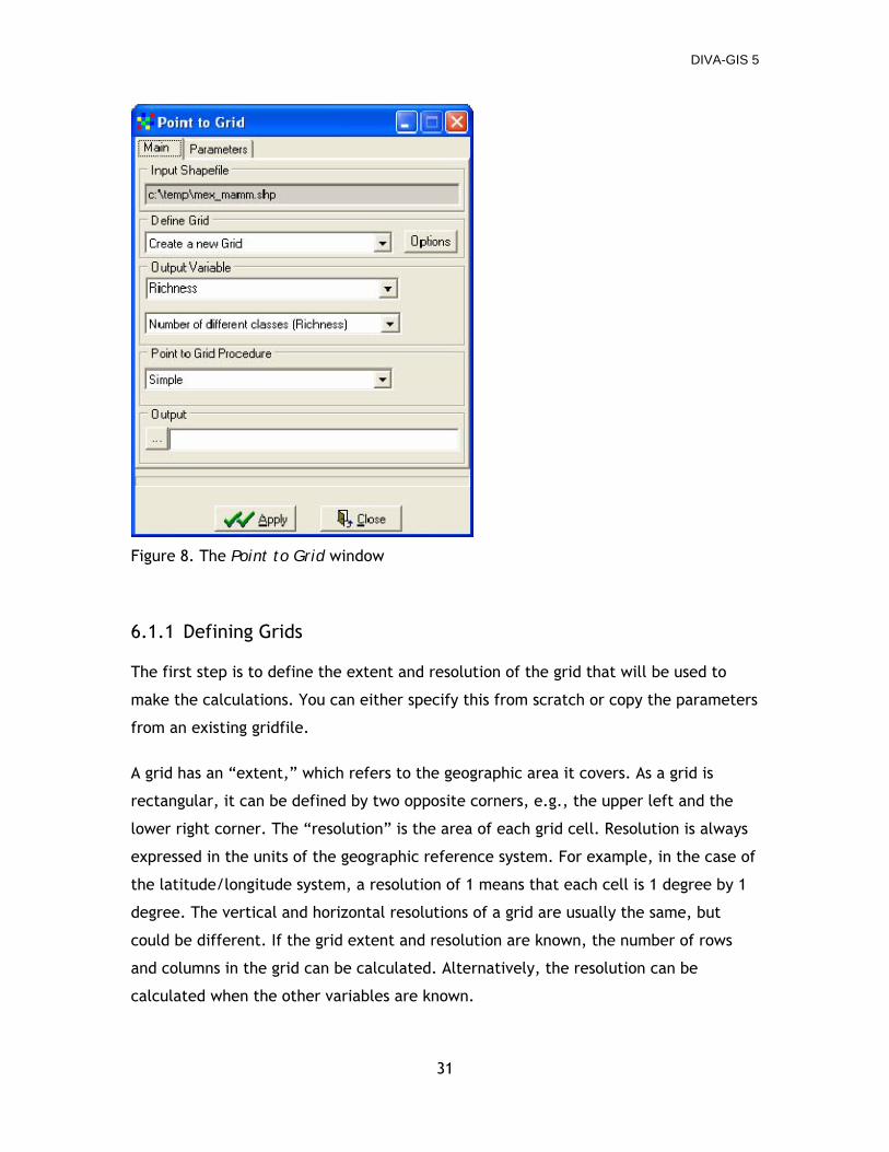
Some of the principal analytical functionality in DIVA-GIS is found in the Analysis/Point
to grid menu. The output of the functions in this window is a grid. When you select
one of the output options (see 7.3), the Point to grid window shown in Figure 8 will
open.
DIVA-GIS 5
31
Figure 8. The Point to Grid window
6.1.1 Defining Grids
The first step is to define the extent and resolution of the grid that will be used to
make the calculations. You can either specify this from scratch or copy the parameters
from an existing gridfile.
A grid has an “extent,” which refers to the geographic area it covers. As a grid is
rectangular, it can be defined by two opposite corners, e.g., the upper left and the
lower right corner. The “resolution” is the area of each grid cell. Resolution is always
expressed in the units of the geographic reference system. For example, in the case of
the latitude/longitude system, a resolution of 1 means that each cell is 1 degree by 1
degree. The vertical and horizontal resolutions of a grid are usually the same, but
could be different. If the grid extent and resolution are known, the number of rows
and columns in the grid can be calculated. Alternatively, the resolution can be
calculated when the other variables are known.
DIVA-GIS 5
32
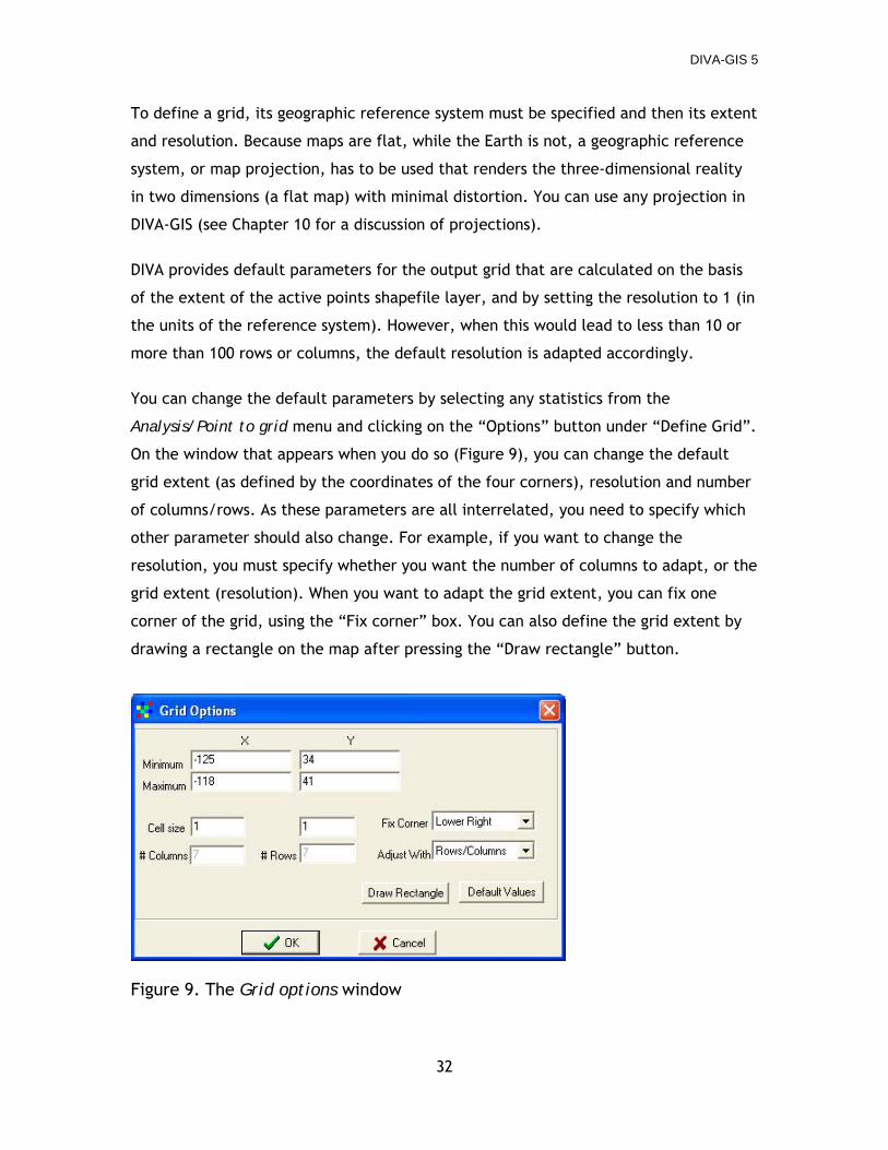
To define a grid, its geographic reference system must be specified and then its extent
and resolution. Because maps are flat, while the Earth is not, a geographic reference
system, or map projection, has to be used that renders the three-dimensional reality
in two dimensions (a flat map) with minimal distortion. You can use any projection in
DIVA-GIS (see Chapter 10 for a discussion of projections).
DIVA provides default parameters for the output grid that are calculated on the basis
of the extent of the active points shapefile layer, and by setting the resolution to 1 (in
the units of the reference system). However, when this would lead to less than 10 or
more than 100 rows or columns, the default resolution is adapted accordingly.
You can change the default parameters by selecting any statistics from the
Analysis/Point to grid menu and clicking on the “Options” button under “Define Grid”.
On the window that appears when you do so (Figure 9), you can change the default
grid extent (as defined by the coordinates of the four corners), resolution and number
of columns/rows. As these parameters are all interrelated, you need to specify which
other parameter should also change. For example, if you want to change the
resolution, you must specify whether you want the number of columns to adapt, or the
grid extent (resolution). When you want to adapt the grid extent, you can fix one
corner of the grid, using the “Fix corner” box. You can also define the grid extent by
drawing a rectangle on the map after pressing the “Draw rectangle” button.
Figure 9. The Grid options window
DIVA-GIS 5
33
6.1.2 Using the parameters of an existing grid
The alternative to defining manually the parameters of a grid is to use the parameters
of an existing grid. You can use the parameters from a gridfile produced in a previous
analysis by scrolling down in the bar in the Define grid option of the Point to grid
window and then pressing “Options” to choose an existing grid. An existing gridfile can
also be used as a “mask” to indicate what part of the grid should be ignored, or should
get special treatment in the case of the Inverse Distance Weighted method (see
section 4.3). The part of the grid that should be ignored can be indicated using
numerical values or ranges.
6.2 Output variables
There are a number of different output variables that can be calculated for a grid. The
output variable you want can be selected under the Point to grid/Main/Output
variable menu. Output variables are grouped, and associated with a number of options
that can be set on the Parameters tab to the right of the Main Tab. The different
output variables are discussed in the following sections.
6.2.1 Richness
In the Richness group there are four distinct output variables: Number of different
classes, Number of observations, Presence/absence and Rarefaction.
Number of different classes counts the different classes of a variable (e.g., the
different species names in a dataset covering a genepool) present in each grid cell.
The Parameters tab must be used to indicate which variable in the shapefile should be
considered, and possibly to exclude irrelevant values.
The Number of observations option calculates the number of points present in each
grid cell. As there may be points in the shapefile that are not relevant, you may want
to exclude these. In that case, you must select a variable from the database on the
Parameters tab (Figure 10), and then you can exclude one or more of the values of
that variable.
DIVA-GIS 5
34
Presence/absence simply gives cells in which a class is found the value 1 and cells in
which it is not found the value 0.
The Rarefaction technique estimates the number of classes (species, for example) that
would have been observed given a number of observations that is specified by the user
(Sanders, 1968; Hurlbert, 1971; Magurran, 1988). Equation 1 gives the formula which is
used to make this calculation.
A disadvantage of this method is that the estimate can only be calculated for those
cells in which the actual number of observations is higher than that for which the
estimate is calculated.
∑⎥⎥⎦
⎤
⎢⎢⎣
⎡
⎭⎬⎫
⎩⎨⎧
⎟⎟⎠
⎞⎜⎜⎝
⎛⎟⎟⎠
⎞⎜⎜⎝
⎛ −−=
nN
nNN
E i /1 (S) (Equation 1)
E(S) – Expected number of classes in the rarefied sample;
N – Total number of observations per cell, in the sample to be rarefied;
Ni – Number of individuals in the i-th class, in the sample to be rarefied;
n – User specified standardized sample size.
DIVA-GIS 5
35
Figure 10. The Parameters tab.
6.2.2 Estimators of Richness
The number of species (or whatever other units) observed in an area depends to some
extent on the effort invested in recording there. Because a complete census is rarely
feasible, in most cases only a sample of an area is surveyed. An important problem
that then arises is to estimate the total species (or other unit) number, Smax, for the
area. This estimate can give both a measure of the completeness of the inventory and
also allow for better (i.e., less biased by the number of observations) comparison with
the species richness of other localities. An estimate of the maximum species number is
also useful when assessing if the further information to be gained from continued
sampling justifies the cost. Various different approaches have been proposed to
estimate Smax. Some of these have been implemented in DIVA-GIS based on the review
by Colwell and Coddington (1994), and later authors.
DIVA-GIS 5
36
Chao 1 Chao (1984) derived a simple estimator (S1 or “Chao-1”) of the true number of species
in an assemblage based on the number of rare species in the sample:
( )baSS OBS 2/21 +=
Sobs is the observed number of species in a sample; a is the number of observed species that are represented by only a single individual in that sample (i.e., the number of singletons); b is the number of observed species represented by exactly two individuals in that sample (the number of ‘doubletons’).
Chao 1 Corrected This corrected version replaces the original Chao estimator (which is still included to
allow for comparison with studies that have used this estimator). The corrected
version is less biased.
Where Sobs is the total number of species observed and Fi is the number of species that have exactly i individuals (F1 is the frequency of singletons, F2 the frequency of doubletons)
Chao 2 Chao 2 is an incidence-based estimator of species richness (Chao 1987). Chao 2 and
the Jacknife estimators are based on the number of samples for an area. To create
samples, DIVA-GIS divides each grid-cell into 4 or 9 sub-areas.
Where Sobs is the total number of species observed in all samples pooled and Qj Number of species that occur in exactly j samples (Q1 is the frequency of uniques, Q2 the frequency of duplicates).
Jacknife “Jacknife 1” is the first-order jacknife estimator of species richness (incidence-based) (Burnham and Overton 1978,1979; Heltshe and Forrester 1983)
.
DIVA-GIS 5
37
“Jacknife 2” is the second-order jacknife estimator of species richness (incidence-based) (Smith and van Belle 1984)
.
Where: Sobs is the total number of species observed in all samples pooled; Qj
the number of species that occur in exactly j samples (Q1 is the frequency of uniques, Q2 the frequency of duplicates). m is the total number of samples
Michaelis-Menten
This estimator is calculated by repetitive random sampling and fitting an asymptotic
model, following the method of Raaijmakers (1987). For each sample size (from 2 to
the number of observations –1), the average number of species in the sample is
calculated over the random samples (the default is 100 samples for each sample size,
but a higher number may be better for some data). The number of species is
estimated from this generated species accumulation curve.
This asymptotic model assumes that the probability that the next individual captured
will be a new species declines linearly with species number, and thus the species
accumulation curve is the negative exponential function:
(Equation 2)
Where k is a fitted constant and n the number of samples.
The asymptotic behavior of the accumulation curve can also be modeled as the
hyperbola:
(Equation 3)
Where Smax and B are fitted constants.
DIVA-GIS 5
38
This is the Michaelis-Menten equation used in enzyme kinetics and thus there is an
extensive literature discussing the estimation of its parameters, which unfortunately
presents considerable statistical difficulties (Colwell and Coddington, 1994). The
method implemented in DIVA-GIS, favored by Raaijmakers (1987), is to calculate Smax
and B using their maximum likelihood estimators as follows:
(Equation 4)
Where Syy, Sxx and Sxy are the sums of squares and cross products of the deviations Y Y i and X X i. S-obs
This is simply the actual number of species observed per grid cell.
6.2.3 Turnover
Turnover (or beta-diversity) is a measure of the rate at which species assemblages
change in space. It indicates how different a number of nearby areas are. Imagine two
large areas with similar numbers of species overall, but one with different species in
all its grid cells and another with the same species in all its grid cells. The first area
would have a high turnover, the second area a low turnover.
At this point, only Whittaker’s (1960) measure of beta-diversity is implemented in
DIVA-GIS (Equation 9). It can be calculated for each grid cell considering its 8
neighbors (2 horizontal, 2 vertical, and 4 diagonal; “Queen’s case”) or considering its 4
closest neighbors (2 vertical and 2 horizontal; “Rook’s case”).
( ) 1/ −= αβ Sw (Equation 5)
S = total number of species over the grid cells considered α = average number of species in the grid cells considered.
DIVA-GIS 5
39
6.2.4 Diversity indices
DIVA-GIS can calculated a number of different diversity indeces for each grid cell. You
must select a variable (field) from the input database for which you want to calculate
an index. The formulas for all indices were taken from Magurran (1988), who provides
a detailed description of their properties. See Table 5 for the mathematical
description of the different diversity indices.
Table 5. Diversity indices
Index Formula
Margalef DMg = (S – 1) / ln(N)
Menhinick DMn = S / √ N
Shannon H’ = –∑ pi ln pi
Simpson D = ∑(ni (ni –1) / N/(N–1))
Brillouin HB = (ln N! – ∑ ln ni!) / N
S – number of unique classes (species) per cell
N – number of observations per cell
ni – number of individuals in the i-th class
pi – proportional abundance of the i th class = ni / N
The Simpson index, D, decreases with increasing diversity, and hence it is usually
expressed as 1–D or 1/D. In DIVA-GIS it is expressed as 1-D. You can use Grid/Scalar to
calculate D or 1/D from this (see Chapter 9).
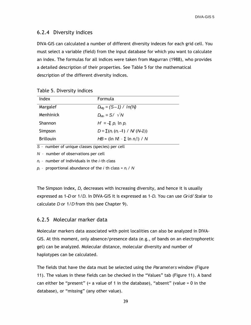
6.2.5 Molecular marker data
Molecular markers data associated with point localities can also be analyzed in DIVA-
GIS. At this moment, only absence/presence data (e.g., of bands on an electrophoretic
gel) can be analyzed. Molecular distance, molecular diversity and number of
haplotypes can be calculated.
The fields that have the data must be selected using the Parameters window (Figure
11). The values in these fields can be checked in the “Values” tab (Figure 11). A band
can either be “present” (= a value of 1 in the database), “absent” (value = 0 in the
database), or “missing” (any other value).
DIVA-GIS 5
40
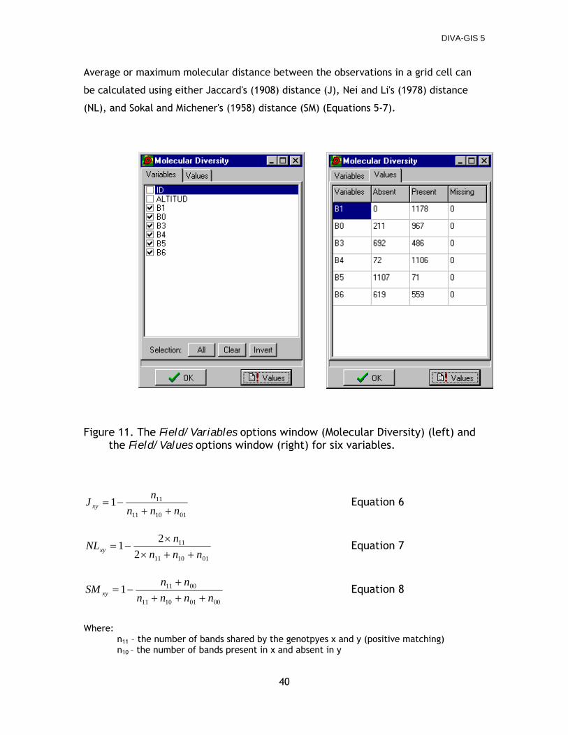
Average or maximum molecular distance between the observations in a grid cell can
be calculated using either Jaccard's (1908) distance (J), Nei and Li's (1978) distance
(NL), and Sokal and Michener's (1958) distance (SM) (Equations 5-7).
Figure 11. The Field/Variables options window (Molecular Diversity) (left) and the Field/Values options window (right) for six variables.
011011
111nnn
nJ xy ++
−= Equation 6
011011
11
221
nnnnNLxy ++×
×−= Equation 7
00011011
00111nnnn
nnSM xy +++
+−= Equation 8
Where:
n11 – the number of bands shared by the genotpyes x and y (positive matching) n10 – the number of bands present in x and absent in y
DIVA-GIS 5
41
n01 – the number of bands present in y and absent in x n00 – the number of bands absent both in x and y (negative matching)
Alternatively, molecular diversity can be calculated using Nei’s diversity index
(Equation 8).
ijij
ji NDIxxNDI ⋅⋅= ∑ Equation 9
Where: xi - the frequency of the i-th allele in the population and NDIij - the number of allele differences per locus between the the i-th and j-th loci
6.2.6 Reserve selection
The Reserve Selection procedure aims to identify sets of grid cells that are
complementary to each other, i.e. that capture a maximum amount of diversity in as
few cells as possible. Instead of using simple richness, an adjustment can be made in
which rare observations get a higher weight.
The procedure is based on the algorithm described by Rebelo (1994) (see also Rebelo
and Sigfried (1992)). It has, for example, been used to determine priority areas for in
situ conservation of species in a family of flowering plants in South Africa. The
following discussion refers to species, but any multi-state variable could be used. The
procedure is less straightforward than it might seem. Whereas the selection of the
first cell is easy – it is the cell with highest species richness (or a random choice
between ties if there are any) – the choice of the next cell(s) depends on the
previously selected cells. This is because the species in the cell with the second
highest number of species may also be present in the first cell. In other words, the cell
with the second highest number of species may not contribute very much to the
overall number of species selected. To maximize the total number of species selected
in as few cells as possible is a non-linear optimization problem. Rebelo (1992)
developed a procedure that calculates an approximate optimal solution, and this is
what has been implemented in DIVA-GIS.
An iterative procedure is used. In each iteration, the “value” of each grid cell is
calculated, based on the observations in that cell, and in relation to the observations
DIVA-GIS 5
42
in the cells already selected. If there are two or more cells with the same “value”,
one is selected at random. Hence, this procedure can lead to slightly different results
every time it is run.
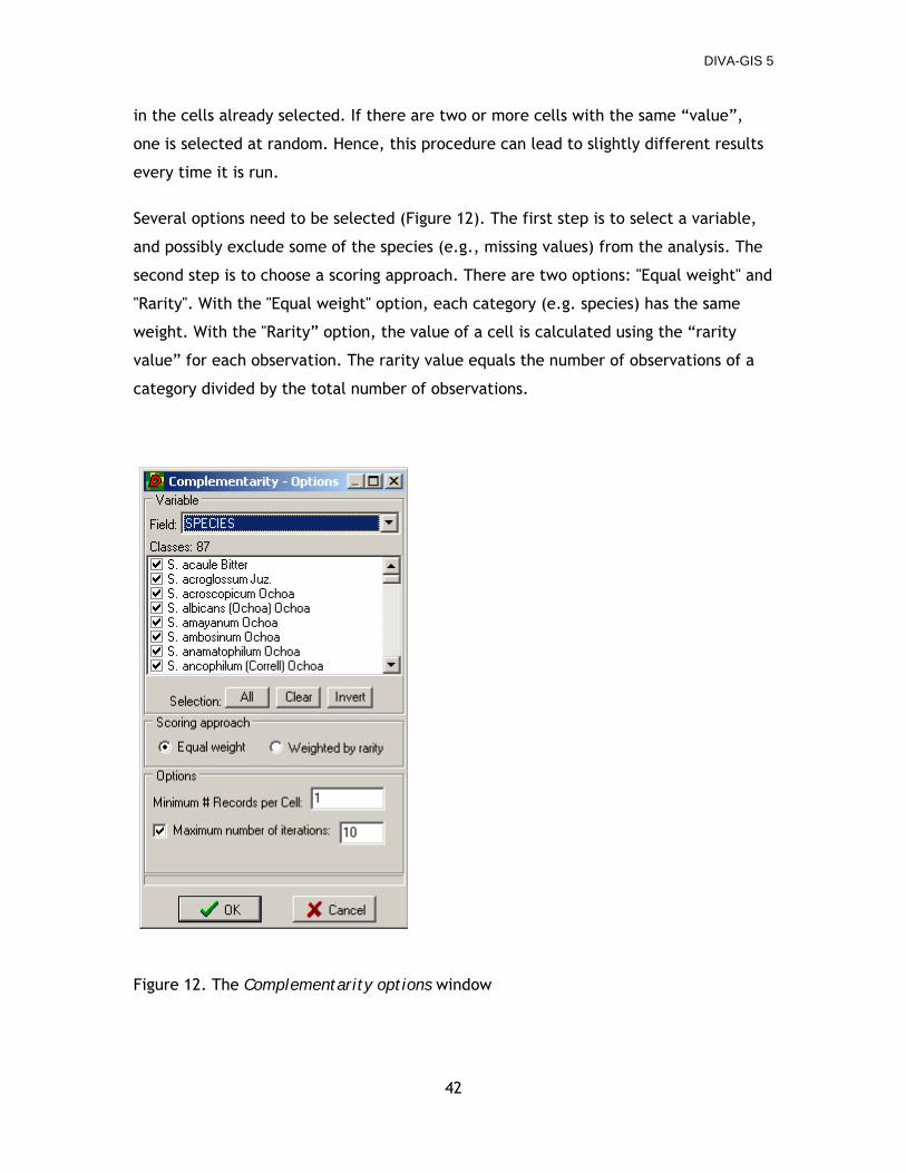
Several options need to be selected (Figure 12). The first step is to select a variable,
and possibly exclude some of the species (e.g., missing values) from the analysis. The
second step is to choose a scoring approach. There are two options: "Equal weight" and
"Rarity". With the "Equal weight" option, each category (e.g. species) has the same
weight. With the "Rarity” option, the value of a cell is calculated using the “rarity
value” for each observation. The rarity value equals the number of observations of a
category divided by the total number of observations.
Figure 12. The Complementarity options window
DIVA-GIS 5
43
There are two ways in which you can limit the number of iterations. This is important
because the procedure can take a long time with large databases (or a grid with a
many cells). You can indicate the "Minimum number of records per cell". This value
should be 1 or higher. It allows you to exclude cells with what is, for your purposes,
too low a number of observations. You can also indicate the maximum number of
iterations that you want the procedure to cycle through.
When the process finishes, a "Process Report" appears, that tells you how many
iterations were used (and hence the number of cells selected) and how many distinct
observations are present in those cells.
Three new grid are created and added to the project, labeled Sequence, Classes and
Additional Classes.
The Sequence grid indicates in which order cells were selected. The cell with most
species is selected first, and has a value of 1. The next cell has a value of 2, etc. The
Classes grid indicates how many different classes (typically species) are in each
selected cells. The Additional Classes grid indicates how many new classes (species)
are in that cell. These species were not present in any of the previously selected cells.
6.2.7 Statistics If a numerical variable is selected, some basic statistics can be calculated for that
variable, for each grid cell. The statistics included are listed in Table 6.
Table 6. Statistics
Coefficient of variation Coefficient of variation of values Maximum Maximum value Mean Mean value Median Median value Minimum Minimum value Mode Mode (most frequent) value Range Difference between Max and Min Range/Mean Range divided by the mean Standard deviation Standard deviation of values Sum Sum of all values Variance Vriance of values
DIVA-GIS 5
44
6.3 Methods of converting point data to grid data
At the core of DIVA-GIS is the conversion of the point data represented by the
accession localities to the raster data represented by the diversity and other values of
the different grid cells. Several GIS programs allow the conversion of point data to
raster data. However, the way that this is generally done (as in the “simple” method
in DIVA-GIS) has the following important shortcomings:
• A point that is on a border between grid cells is assigned to one of those cells
arbitrarily;
• The value of a point that falls within a grid cell is assigned to that cell only,
irrespective of the proximity of the point to other cells;
• The origin of the grid (i.e. its bottom left-hand corner) is arbitrary. Given a
coordinate system and resolution of the grid, slightly different origins could
lead to quite different results of the point-to-grid conversion;
• Uncertainty about the location of points is not taken into account.
These shortcomings can largely be overcome with the “circular neighborhood” and
“inverse distance-weighted” (IDW) techniques, as implemented in DIVA-GIS for the
Point to grid procedure and described below.
6.3.1 Circular neighborhood
When the Circular neighborhood option is chosen in Analysis/ Point to grid/Main,
calculations are made based not on the observations within each grid cells but rather
on the observation found within a circle with its center in the middle of each grid cell
and of a specified radius. The advantage of this method is that it produces a smoother
surface. To avoid some observations not being used at all, the radius should not be
smaller than the distance between the center of a square grid cell and its corners. A
disadvantage may be that a number of observations (or even all, if the radius is
sufficiently large compared to the size of the grid cells) will used more than once in
the calculations. See Bonham-Carter (1994) and Cressie (1991) for more information on
circular neighborhoods.
DIVA-GIS 5
45
When this method is used, you must specify in the Options tab the size of the
neighborhood (i.e., the diameter of the circle), and indicate if you want to scale the
result. Scaling means you correct the results for the difference between the size of
the grid cell and that of the neighborhood.
6.4 Point to polygon
Polygons, or closed lines that enclose an area, can also be used to summarize point
distribution data. For example, you may want to make calculations for different
countries.
Make a shapefile of points the active theme and click on Analysis/Point to
polygon/Diversity. Then specify which polygons are going to be used to make the
calculations. You can either select an existent shapefile (e.g. with administrative
boundaries or ecoregions) or define a new shapefile of squares (i.e., a grid) or
hexagons. Note that if you define a grid of squares you will get the same output as
with Point to grid, except for minor differences due to the way points that fall on the
borders between two cells are treated.
The output consists of a shapefile with the following fields:
DIVAID and ORDER – these can be ignored.
OBS - the number of observations;
SPP - the number of different classes, typically species:
Four diversity indices: Margalef, Menhinick, Shannon, Simpson (see section 7.3.3;
Table 5).
The value “-1” in the Simpson column means “missing value” (i.e., the index could not
be calculated).
As the size of polygons may vary, unlike grid cells, the results may need careful
interpretation. Nevertheless, this can be an interesting option that allows
summarizing the data by pre-defined, and often well-known, areas.
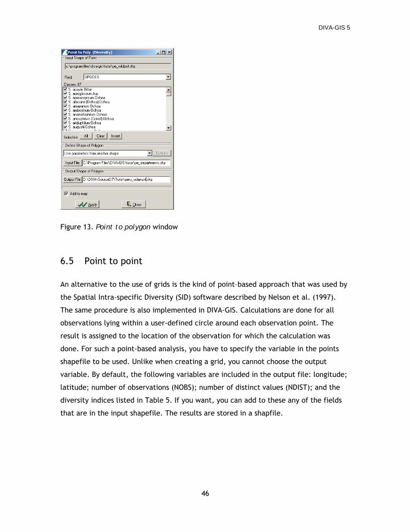
DIVA-GIS 5
46
Figure 13. Point to polygon window
6.5 Point to point
An alternative to the use of grids is the kind of point–based approach that was used by
the Spatial Intra-specific Diversity (SID) software described by Nelson et al. (1997).
The same procedure is also implemented in DIVA-GIS. Calculations are done for all
observations lying within a user-defined circle around each observation point. The
result is assigned to the location of the observation for which the calculation was
done. For such a point-based analysis, you have to specify the variable in the points
shapefile to be used. Unlike when creating a grid, you cannot choose the output
variable. By default, the following variables are included in the output file: longitude;
latitude; number of observations (NOBS); number of distinct values (NDIST); and the
diversity indices listed in Table 5. If you want, you can add to these any of the fields
that are in the input shapefile. The results are stored in a shapfile.
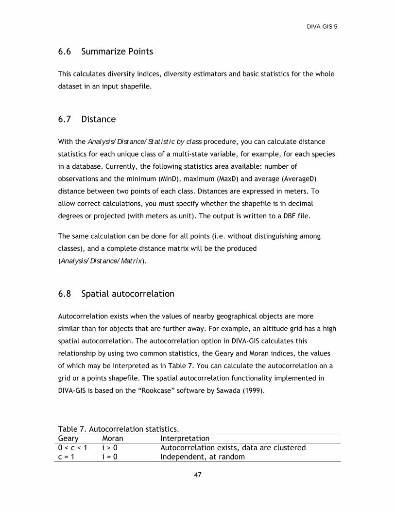
DIVA-GIS 5
47
6.6 Summarize Points
This calculates diversity indices, diversity estimators and basic statistics for the whole
dataset in an input shapefile.
6.7 Distance
With the Analysis/Distance/Statistic by class procedure, you can calculate distance
statistics for each unique class of a multi-state variable, for example, for each species
in a database. Currently, the following statistics area available: number of
observations and the minimum (MinD), maximum (MaxD) and average (AverageD)
distance between two points of each class. Distances are expressed in meters. To
allow correct calculations, you must specify whether the shapefile is in decimal
degrees or projected (with meters as unit). The output is written to a DBF file.
The same calculation can be done for all points (i.e. without distinguishing among
classes), and a complete distance matrix will be the produced
(Analysis/Distance/Matrix).
6.8 Spatial autocorrelation
Autocorrelation exists when the values of nearby geographical objects are more
similar than for objects that are further away. For example, an altitude grid has a high
spatial autocorrelation. The autocorrelation option in DIVA-GIS calculates this
relationship by using two common statistics, the Geary and Moran indices, the values
of which may be interpreted as in Table 7. You can calculate the autocorrelation on a
grid or a points shapefile. The spatial autocorrelation functionality implemented in
DIVA-GIS is based on the “Rookcase” software by Sawada (1999).
Table 7. Autocorrelation statistics. Geary Moran Interpretation 0 < c < 1 c = 1
i > 0 i = 0
Autocorrelation exists, data are clustered Independent, at random
DIVA-GIS 5
48
c > 1 i < 0 Negative autocorrelation
6.8.1 Points
Autocorrelation for points is calculated point by point, and you need to define which
neighboring points to consider. This is done by specifying the lag (or neighborhood)
distance. Only points within the lag distance are considered for calculation.
To determine a reasonable lag distance, a number of statistics are shown in the
Options tab of the Analysis/Autocorrelation/Points window. These statistics include
the number of observations (points) and statistics describing the distances among all
pairs of points (min, max, mean, median and first and third quartile).
You must select a quantitative field from the shapefile’s database to calculate
autocorrelation. After selecting a field you can deselect individual values that you
want to exclude. If you do that you need to recalculate the statistics, which will have
changed, because you do no longer consider all points. The results will appear on
clicking Apply.
Figure 14. Point autocorrelation screen (Options, left and Results, right)
DIVA-GIS 5
49
6.8.2 Grid
No lag distance needs to be specified to calculate autocorrelation of grids. Only
adjacent cells are considered, either 4 horizontally and vertically adjacent cells
(”Rook’s case”), or also including the 4 diagonally adjacent cells (”King’s case”).
6.9 Histogram
With the Histogram option your grid data are arranged in classes. The program offers
you some common tools to improve the histogram (titles, show grid, etc.) and the
result can be copied to the clipboard.
6.10 Regression
With the Regression tool, you can regress one grid against another (cell by cell) and
plot the results. Choose one gridfile for X and another for Y, make sure that the grid
extents and resolutions coincide. You can use linear, logarithmic, or exponential
regression.
6.11 Multiple Regression
You can regress one grid against several others using the Multiple regression tool. If
you find a satisfactory (statistically significant) model, you can use it to predict values
for the same area, or for another area (by changing the independent variables).
DIVA-GIS 5
50
7. THE MODELING MENU
The Modeling menu provides various options for niche modeling, or the prediction of
species distribution patterns.
Box 8. Functions in the Modeling menu
Icon Sect. Name Short explanation
7.1 Bioclim / Domain Runs the BIOCLIM and DOMAIN models for predicting
the presence of species
7.2 External Models Use other models to predict the presence of species
7.3 Evaluation
7.5 EcoCrop Predicts the adaptation of a crop for a selected area
7.6 Terrain Modeling
7.1 Bioclim / Domain
With the Bioclim / Domain tool you can extract data from the climate database for
point locations (in the active points shapefile), make graphs of these data and use the
extracted data for predictive niche modeling using the BIOCLIM (Busby, 1991; Nix,
1986) and the DOMAIN (Carpenter et al., 1993) approach.
You can only open this window when a points shapefile is the active layer on your
Table of contents. There are six tabs in this window:
7.1.1 Input
Here you can choose to run a model with the standard climate data (DIVA climate
data) or with a stack of layers of your choosing.
and choose to consider all points as one class (e.g., species) or distinguish different
classes by selecting an appropriate field. Duplicate points (with exactly the same
coordinates and species) are removed from the analysis. You can choose whether you
want to also remove points that fall within the same grid cell (this is recommended).
DIVA-GIS 5
51
7.1.2 Frequency
You can make cumulative frequency distribution plots for various climatic variables,
for up to two classes, which are shown in different colors on the graph. This can be
very useful in spotting outliers, which may be due to errors in the data. Click on a
point on the graph (for the second class only) to see where the corresponding locality
is on the map, and display attribute and/or climate data for that point. You can show
percentiles and the 1.5 * inter-quartile range (IQR; points within this range are not
considered outliers) on the graphs, and change the size of the dots. You can save the
graph to the clipboard with the “Copy” button (and then paste it into a document or
presentation) and counts of the number of observations per class to a TXT file (“Save
Stats” button).
7.1.3 Outliers
Here you find outliers in environmental space. You can include 1 to n variables in the
evaluation (n being the number of variables in your stack; if you use diva climate files
n =19). Suspect records are colored red. You can click on a line on the graph to see
where the corresponding locality is on the map, and display attribute and/or climate
data for that point.
7.1.4 Histogram
Another way to explore the climate data for a points shapefile is to make histograms.
Select a class, a variable and either an appropriate bar width or number of bars. You
can restrict the minimum and maximum values to be shown. As usual, you can save the
histogram to the clipboard.
7.1.5 Envelope
In this menu, you must choose a class (i.e. species) and two climatic variables. On
pressing the “Apply” button, a graph will be drawn in which each point on the graph
represents the climate of a point on the map, each axis representing one of the
climate variable that you chose (Figure 17).
DIVA-GIS 5
52
You can set a percentile value to find out which are the extreme observations in terms
of climate. The percentile is used to exclude the extreme values of all climate
variables. A box is drawn on the graph to indicate, for the two climate variables
selected, which points are within, and which points are outside the climatic
“envelope” defined by the specified percentiles. These points will be different for
each pair of variables.
The points that fall within the envelopes for all the climate variables are colored
green on the graph. The points that fall outside one or more envelopes are shown in
red. All the points inside the two-dimensional envelope shown on the graph are
‘selected’ (highlighted in yellow) on the map. You can of course save the graph to the
clipboard in the usual way. The “Extract” button saves a TXT file with the average
values of each bioclimatic variable for each class.
7.1.6 Predict
This is the business end of this menu. The extracted climate data can be used to
predict where a species is likely to occur, or would survive if it was brought there (this
could be on a different continent, for example).
To select an area for mapping, you can enter the coordinates manually, or you can
press the “Read dimensions” button, and the dimensions of the active layer will be
copied. These may need to be adjusted a little to coincide with those of the climate
database. This is done automatically, but you can also do it by pressing the “Adjust”
button.
You can select the climate variables you want to use in the analysis. The fewer
variables you select, the larger the predicted areas of suitability will be. You can also
choose either the current climate or the future climate.
If you selected “Many classes” on the Options tab, you can use the “Batch” option
under Predict to run the model for all different classes (typically species). Or you can
select a single class and run the model for that only.
You must select an name an output grid. You have a choice of six different output
variables for this grid:
DIVA-GIS 5
53
Bioclim - Four types of areas are mapped. Areas completely outside the 0-100
percentile envelope for one or more climate variables get a code “0”. The cells within
the 5-95 percentile get a code “3”, those outside this range but within the 2.5-97.5
percentile get a code “2”, and the ones outside this but within the 0 -100 percentile
for all climate variables get a code “1”.
Bioclim True/False – All areas that are within the envelope described by the data
points, cut off beyond a certain user defined percentile, are mapped as “true” (1); all
other areas are mapped as “false” (0).
Bioclim most limiting factor – For the cells that fall within the 0-100 percentile, the
variable for which the percentile score was lowest (or highest) is mapped. The value in
each grid square is a number that corresponds with the variables on the Predict tab
(Figure 18).
Domain - The Domain procedure calculates the Gower distance statistic between each
cell on the map and each point, using the values of the 19 climate variables. The
distance between point A and grid cell B for a single climate variable is calculated as
the absolute difference in the values of that variable divided by the range of the
variable across all points. The Gower distance is then the mean over all climate
variables.
∑=
−=
p
k
kkAB krange
BAp
d1 )(
||1
The Domain similarity statistic is calculated as
ABdD −= 1
The maximum similarity between a grid cell and all points is mapped. In DIVA, this
value is then multiplied by 100. A good match is thus a high number (e.g., above 95).
Domain (mean distance)
Same as above but the mean distance to all points is used instead of the minimum
distance.
DIVA-GIS 5
54
Domain true/false All areas that are within the specified threshold are mapped as
“true” (1); all other areas are mapped as “false” (0).
Domain most limiting factor The variable with the lowest score (largest distance) is
mapped. The value in each grid square is a number that corresponds with the order of
the variables on the Predict tab.
7.2 External Models
With this module you can export points from a shapefile to prepare input files for
‘external’ distribution models. In some cases, such as for MAXENT and GARP, this is in
fact not very difficult, because they just use a list of species with coordinates.
However, for programs that need a site x species matrix (such as GRASP), the
preparation of input files is far from trivial. For GRASP, 3 files are made (YYY, XXX,
and XXXpred).
Some models will produce grids in a format that DIVA can import via the Data / Import
to gridfile menu. GRASP, however, produces LookUp Tables, or LUT files that can be
imported in this module. You must select the LUTs you want, together with the stack
that was used to make the input files (or another, but compatible, stack, if you study
climate change).
7.3 Evaluation
7.3.1 Prepare points
This tool allows you to split point distribution data into a number of subsets that you
can use to train or test a distribution model. You can specify what percentage of the
points you want to use to 'train' (=run) the model (as a percentage of the total number
of points: “Sample size training data”), and how many separate times you want to do
the sampling (“# repetitions”) (i.e., the number of times you want to run a single
model. You can also sample the background environment to create ‘pseudo-absence’
points. The output is two shapefiles of points, one ending on "_train" (the model
training data, and another on "_test" (the model testing data). Use the training data to
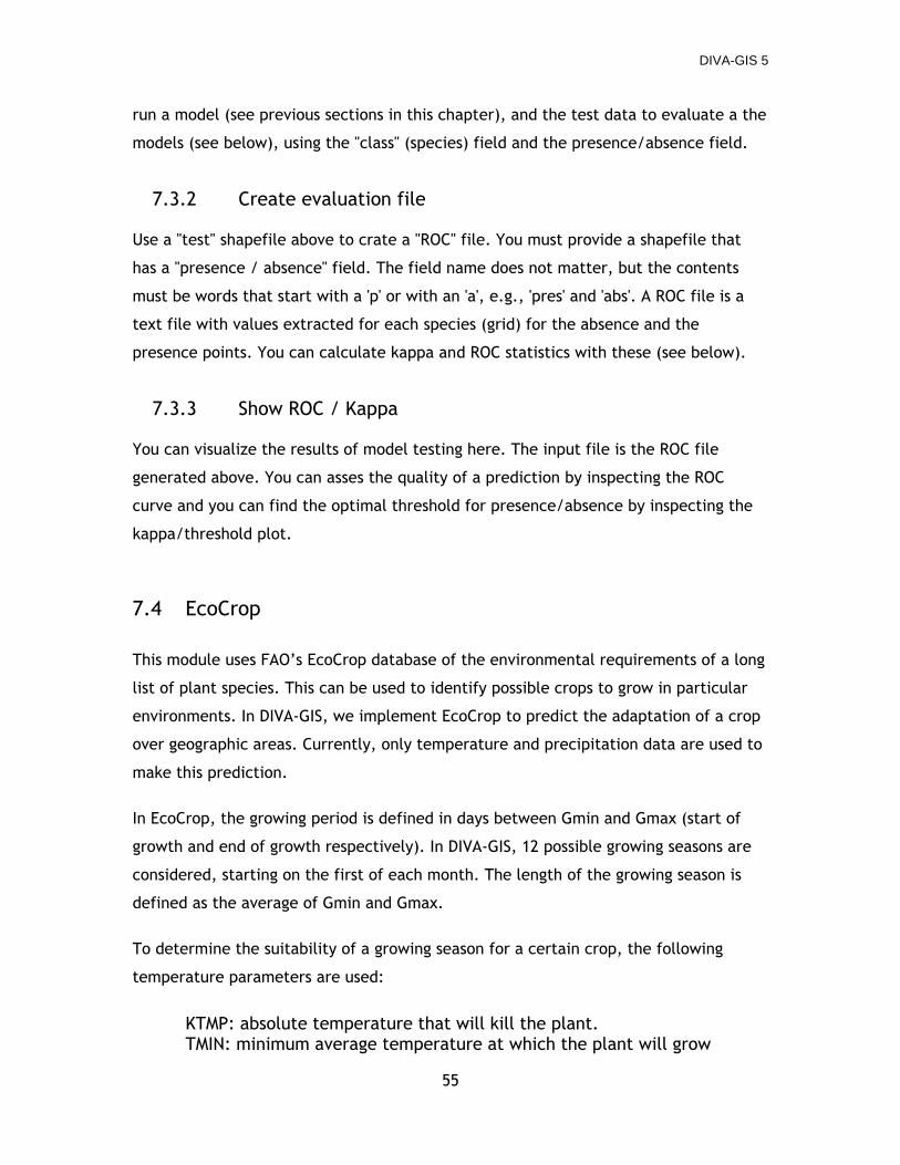
DIVA-GIS 5
55
run a model (see previous sections in this chapter), and the test data to evaluate a the
models (see below), using the "class" (species) field and the presence/absence field.
7.3.2 Create evaluation file
Use a "test" shapefile above to crate a "ROC" file. You must provide a shapefile that
has a "presence / absence" field. The field name does not matter, but the contents
must be words that start with a 'p' or with an 'a', e.g., 'pres' and 'abs'. A ROC file is a
text file with values extracted for each species (grid) for the absence and the
presence points. You can calculate kappa and ROC statistics with these (see below).
7.3.3 Show ROC / Kappa
You can visualize the results of model testing here. The input file is the ROC file
generated above. You can asses the quality of a prediction by inspecting the ROC
curve and you can find the optimal threshold for presence/absence by inspecting the
kappa/threshold plot.
7.4 EcoCrop
This module uses FAO’s EcoCrop database of the environmental requirements of a long
list of plant species. This can be used to identify possible crops to grow in particular
environments. In DIVA-GIS, we implement EcoCrop to predict the adaptation of a crop
over geographic areas. Currently, only temperature and precipitation data are used to
make this prediction.
In EcoCrop, the growing period is defined in days between Gmin and Gmax (start of
growth and end of growth respectively). In DIVA-GIS, 12 possible growing seasons are
considered, starting on the first of each month. The length of the growing season is
defined as the average of Gmin and Gmax.
To determine the suitability of a growing season for a certain crop, the following
temperature parameters are used:
KTMP: absolute temperature that will kill the plant. TMIN: minimum average temperature at which the plant will grow
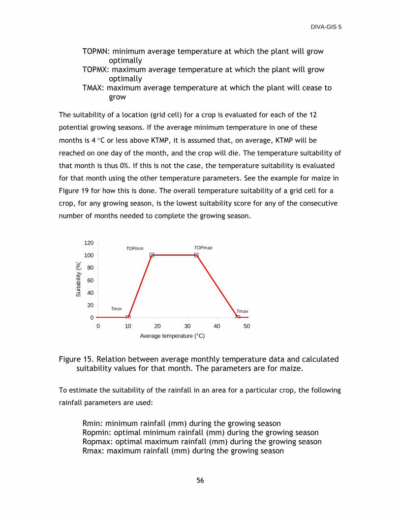
DIVA-GIS 5
56
TOPMN: minimum average temperature at which the plant will grow optimally
TOPMX: maximum average temperature at which the plant will grow optimally
TMAX: maximum average temperature at which the plant will cease to grow
The suitability of a location (grid cell) for a crop is evaluated for each of the 12
potential growing seasons. If the average minimum temperature in one of these
months is 4 °C or less above KTMP, it is assumed that, on average, KTMP will be
reached on one day of the month, and the crop will die. The temperature suitability of
that month is thus 0%. If this is not the case, the temperature suitability is evaluated
for that month using the other temperature parameters. See the example for maize in
Figure 19 for how this is done. The overall temperature suitability of a grid cell for a
crop, for any growing season, is the lowest suitability score for any of the consecutive
number of months needed to complete the growing season.
Figure 15. Relation between average monthly temperature data and calculated suitability values for that month. The parameters are for maize.
To estimate the suitability of the rainfall in an area for a particular crop, the following
rainfall parameters are used:
Rmin: minimum rainfall (mm) during the growing season Ropmin: optimal minimum rainfall (mm) during the growing season Ropmax: optimal maximum rainfall (mm) during the growing season Rmax: maximum rainfall (mm) during the growing season
0
20
40
60
80
100
120
0 10 20 30 40 50
Average temperature (°C)
Suita
bilit
y (%
)
Tmin Tmax
TOPmaxTOPmin
DIVA-GIS 5
57
The evaluation for rainfall is similar as for temperature, except that there is no
“killing” rainfall and there is one evaluation for the total growing period (the number
of months defined by Gmin and Gmax) and not for each month. See Figure 20 for an
example. The output is the highest suitability score (percentage) for a growing season
starting in any month of the year.
You can run the Ecocrop module for rainfall, or for temperature, or for both (the
boxes to tick are in the Predict tab). In the last case, the minimum value of the two
for each growing season is used to compute the suitability.
To run the module you must first select a species in the Select tab. You can search for
species using the options in Filter by. Then select the crop you want by clicking on it
(the selected record is highlighted in blue). On the next tab, Parameters, you can
inspect the temperature and rainfall parameters from the EcoCrop database, and
change them if you want. The changed parameters will be used, but not saved. If you
want to make permanent changes you must edit the file “faoecocrop.dbf” in the
<divadir>\bin directory.
You can select the area for which you want output by filling the upper text boxes on
the Predict tab. You can also use the extent of a shapefile or gridfile by making it
active in the legend and then pressing the “Read from layer” button. The coordinates
need to be adjusted to those of the climate grid cells. You can do this by pressing the
“Adjust coordinates” button. If you do not do this, the program will do it when you
press “Apply”. You can run the EcoCrop module for current and for future climate (see
section 8.1). You must name an output gridfile.
0
25
50
75
100
0 500 1000 1500 2000
Rainfall (mm)
Sui
tabi
lity
(%)
Rmin Rmax
ROPmaxROPmin
DIVA-GIS 5
58
Figure 16. Relation between rainfall during the growing season and calculated rainfall
suitability values for that month. The parameters are for maize.
7.5 Terrain Modeling
Create grids of aspect or slope from an elevation grid (DEM).
DIVA-GIS 5
59
8. THE GRID MENU
Various functions are available in the Grid menu which allow you to create new grids
from one or more existing ones. They are listed in Box 10.
Box 9. The Grid menu
Icon
Sect. Name Short explanation
8.1 Describe Describes the contents and structure of a grid 8.2 Overlay Arithmetic on the values of corresponding grid cells
in two grids 8.3 Scalar Arithmetic on a single grid
8.4 Reclass Classifies the values of a grid in a new way
8.5
Neighborhood Carries out neighborhood operations such as filter
and pattern analysis 8.6 Calculate Arithmetic with multiple grids
8.7 Aggregate Aggregates (combines) cells of a grid
8.8 Disaggregate Disaggregates (divides) cells of a grid
8.9 Cut Cuts a specified section out of a grid
8.10 Concatenate Combines two grids into one
8.11 New
Makes a new grid with the same parameters as an existing one but different cell values
8.12 Transect Makes a graph of the values in a given column or row of a grid
8.13 Area Calculates the area of classes in a g rid
8.1 Describe
You can use this function to get the following information on the contents and
structure of a grid:
Structure: type of data (integer, real), number of rows, number of columns.
DIVA-GIS 5
60
Contents (across all cells): number of cells with data, number of grid cells without
data, minimum value, maximum value, sum, mean, mode, median, variance, and
standard deviation of grid cell values.
Describe operates on the active layer when the window is open, or else on any layer
selected using the “Input file” button. Some of the information (e.g., the number of
rows and columns) can also be obtained by double-clicking on a grid layer in the
legend (and choosing the “Info” tab).
8.2 Overlay
Given two grids that have the same dimensions (number of columns and rows,
resolution), and location (min and max x and y coordinates), Overlay allows you to
place them on top of each other (as it were), carry out some arithmetic on
corresponding grid cells (i.e., cells directly above each other), and place the results in
a new, third grid. The arithmetical operations included are addition, subtraction,
multiplication, division and calculation of minimum and maximum. In the operation
“Cover”, the values of the cells in the first grid are used, unless the value of a cell in
the first grid is “Nodata”, in which case the value of the cell in the second grid is
used.
8.3 Scalar
Scalar lets you create a new grid by applying an arithmetical operation to the values in
each cell of an existing grid. For the following operations you need to also specify a
number: add, substract, multiply, divide, raise to a power, or take the the logarithm
with a specified base. Other functions included are taking the absolute value,
rounding, truncating and trigonometric operations.
8.4 Reclass
The Reclass option re-classifies data in a grid according to class limits which you
specify. For example, you may want to give all grid cells with values between 0 and
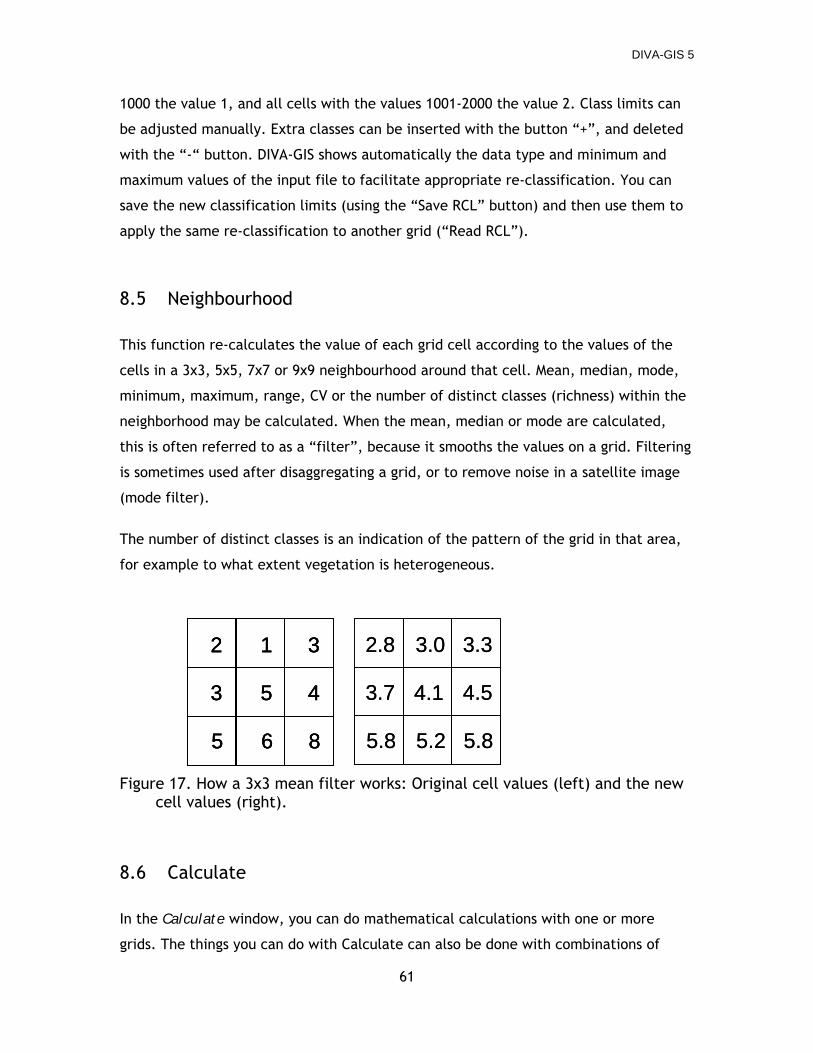
DIVA-GIS 5
61
1000 the value 1, and all cells with the values 1001-2000 the value 2. Class limits can
be adjusted manually. Extra classes can be inserted with the button “+”, and deleted
with the “-“ button. DIVA-GIS shows automatically the data type and minimum and
maximum values of the input file to facilitate appropriate re-classification. You can
save the new classification limits (using the “Save RCL” button) and then use them to
apply the same re-classification to another grid (“Read RCL”).
8.5 Neighbourhood
This function re-calculates the value of each grid cell according to the values of the
cells in a 3x3, 5x5, 7x7 or 9x9 neighbourhood around that cell. Mean, median, mode,
minimum, maximum, range, CV or the number of distinct classes (richness) within the
neighborhood may be calculated. When the mean, median or mode are calculated,
this is often referred to as a “filter”, because it smooths the values on a grid. Filtering
is sometimes used after disaggregating a grid, or to remove noise in a satellite image
(mode filter).
The number of distinct classes is an indication of the pattern of the grid in that area,
for example to what extent vegetation is heterogeneous.
Figure 17. How a 3x3 mean filter works: Original cell values (left) and the new cell values (right).
8.6 Calculate
In the Calculate window, you can do mathematical calculations with one or more
grids. The things you can do with Calculate can also be done with combinations of
12 3
53 4
65 8
3.02.8 3.3
4.13.7 4.5
5.25.8 5.8
12 3
53 4
65 8
12 3
53 4
65 8
3.02.8 3.3
4.13.7 4.5
5.25.8 5.8
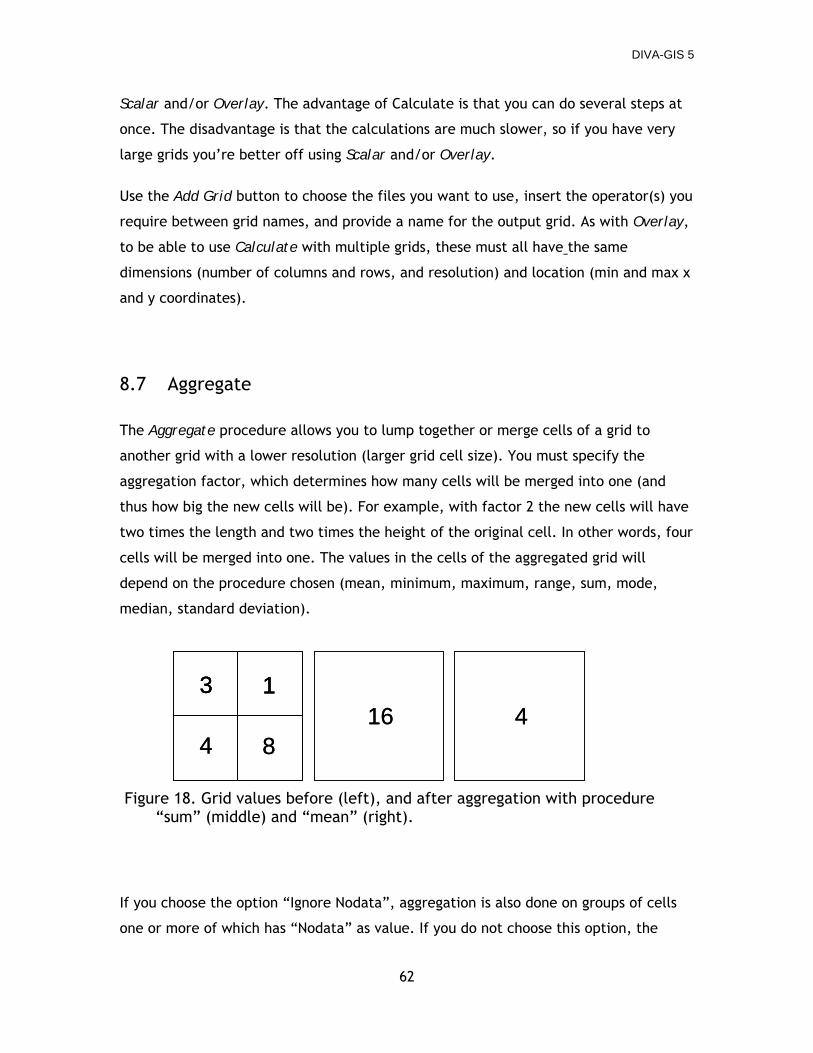
DIVA-GIS 5
62
Scalar and/or Overlay. The advantage of Calculate is that you can do several steps at
once. The disadvantage is that the calculations are much slower, so if you have very
large grids you’re better off using Scalar and/or Overlay.
Use the Add Grid button to choose the files you want to use, insert the operator(s) you
require between grid names, and provide a name for the output grid. As with Overlay,
to be able to use Calculate with multiple grids, these must all have the same
dimensions (number of columns and rows, and resolution) and location (min and max x
and y coordinates).
8.7 Aggregate
The Aggregate procedure allows you to lump together or merge cells of a grid to
another grid with a lower resolution (larger grid cell size). You must specify the
aggregation factor, which determines how many cells will be merged into one (and
thus how big the new cells will be). For example, with factor 2 the new cells will have
two times the length and two times the height of the original cell. In other words, four
cells will be merged into one. The values in the cells of the aggregated grid will
depend on the procedure chosen (mean, minimum, maximum, range, sum, mode,
median, standard deviation).
Figure 18. Grid values before (left), and after aggregation with procedure “sum” (middle) and “mean” (right).
If you choose the option “Ignore Nodata”, aggregation is also done on groups of cells
one or more of which has “Nodata” as value. If you do not choose this option, the
3 1
4 816 4
3 13 1
4 816 4
DIVA-GIS 5
63
value of the aggregated cells will become “Nodata” even if only one of its component
cells has that value.
In some cases, the aggregation factor is not a multiple of the number of rows or
columns. Say you have a grid of 3 by 3 cells that you want to aggregate with a factor
two. In this case, the cells in the last column and row cannot be aggregated properly.
DIVA-GIS gives you two options to deal with this: either ignore these cells and truncate
the original grid (in the example, the aggregated grid would have one cell), or expand
the grid by adding another row and column with Nodata values (in the example, the
aggregated grid would have four cells).
8.8 Disaggregate
Disaggregate divides the cells of a grid into smaller cells. The value of the original cell
is assigned to all of the smaller cells. You need to specify the disaggregation factor,
which should be an integer greater than one.
8.9 Cut
Cut allows you to make a new grid that has only a part of the area of an existing grid.
You can define the area to be cut and placed in the new grid by the column and row
numbers, or by coordinates. These parameters can also be selected by drawing a
rectangle on the map. They can also be copied from an existing grid.
8.10 Concatenate
Concatenate combines the data of two grids with the same resolution and origin, but
with different extents. For areas where both grids have values, the value of the first
grids is maintained (as with Cover).
DIVA-GIS 5
64
8.11 New
You can generate a new grid with this option, using the parameters from an existing
grid. The grid cell values can be a single number, consecutive numbers starting at 0,
or random numbers from a uniform or a Normal distribution.
8.12 Transect
Choose a row or column in a specified grid (either by specifying its number or by
clicking on the grid on the map), and you get a graph showing on the vertical axis the
changes in grid cell values with latitude or longitude. You can choose to fix the
vertical axis so that different transects will be comparable. A moving average will be
displayed if you tick the appropriate box.
The results may be saved in a number of ways. You can save both the graph and the
data on which it is based in the clipboard. You can also save the data to a file by going
to the “Data” tab and specifying an output file.
8.13 Area
Area lets you create a new grid in which the value in each cell represents the total
area of the class in that cell in an existing grid.
DIVA-GIS 5
65
9. THE STACK MENU
A stack is a set of grids with the same dimensions (number of columns and rows, and
resolution) and location (minimum and maximum x and y coordinates) which are
handled together as a group. Grouping grids in a stack makes it easier to process many
files in the same way, and allows a number of additional analytical procedures. You
can carry out the following grid operations (i.e. from the Grid menu, see section 8) on
stacks as well individual grids: Scalar, Reclass, Neighbourhood, Aggregate,
Disaggregate, Cut, Distance and Area.
A stack is stored in a file with the extension GRS. A GRS file is nothing but a list of the
grids that the stack contains. Hence, it does not contain any of the actual data in the
grids, rather it points at the existing files with the data. Therefore, if you delete,
rename, or move one its constituent grids to a different directory, the stack will
become invalid.
Box 10. The Stack menu
Sect. Name Short explanation 9.1 Make Stack Defines a stack by listing the grids it contains 9.2 Plot Makes a histogram of cell values 9.3 Calculate Carries out arithmetic on grids in a stack 9.4 Regression Calculates regression on a cell by cell basis 9.5 Cluster Classifies grid cells 9.6 Export to textfile Places all grid cells values in a single text file
9.1 Make stack
You make a stack by adding grids to a list and then naming the output GRS file. You
can remove grids from the list individually or all at once if you make a mistake or
change your mind. DIVA tells you about the dimensions and location of each grid you
add to the stack. These must be identical for all grids in the stack. If you forget which
grids are in a stack, or wonder whether it is still valid, or why it isn’t, use the “Check
Stack” tab to obtain a list of the grids included in a specified stack. You can edit stack
files with text editors such as Notepad.
DIVA-GIS 5
66
9.2 Plot
With this, you can make a histogram of the values in corresponding cells in all grids in
a stack.
9.3 Calculate
Using Calculate, you can produce a single grid from the multiple grids in a specified
stack, the value in each cell of the output grid being the sum, mean, minimum,
maximum, harmonic mean or sum of the reciprocals of the values in the grids in the
stack.
If you select the “Calculate Area” option, a text file is produced with the area of each
grid (expressed as number of cells) with values above a certain specified threshold
value. If you select a grid to serve as a ‘mask’, only the cells for which the mask has
data (i.e., not “Nodata”) will be considered.
9.4 Regression
You can use this function to perform regression on a cell basis, across a stack of n
grids. That is, for each cell position, linear regression is done using 1…n as X values
and the values in the corresponding grids as Y values. Make sure that the grids are in
the right order. You can open the stack file with a text editor and check.
9.5 Cluster
You may want to classify grid cells based on the values they have in different grids, for
example if the different grids represent the presence and absence of different
species. You can do this in the Cluster menu in three steps:
1. In the “Distance Matrix” tab, calculate a matrix of distances (file extension DMT)
between grid cells by specifying a distance measure.
DIVA-GIS 5
67
2. In the “Cluster” tab, use the DMT file produced above to calculate a cluster file
(file extension DTR) using either the weighted or unweighted UPGMA algorithm.
3. In the “Draw” tab, use the DTR file you just produced to draw a dendrogram of the
distance relationships among grid cells, decide at what level of distance to prune the
dendrogram, and finally produce a new grid in which the values of the grid cells will
correspond to which cluster in the dendrogram the cells belongs to.
9.6 Export to textfile
With the option Export to textfile, all the gridfiles in the stack can be exported
together to a single TXT file. Such a file can be used to make comparisons on a cell-
by-cell basis, e.g. in a spreadsheet program. As an option, any row that has a null
value for one or more of the grids may be omitted in the output file.
DIVA-GIS 5
68
10. THE TOOLS MENU
The Tools menu (Box 11) has some additional miscellaneous functions.
Box 11. The Tools menu
Icon Sect. Name Short explanation
10.1 Projection Projects a shapefile from geographic coordinates to
a projection of choice Graticule 10.2 Shift shape Shifts the position of a shapefile
10.3 Georeference
image Tools to help you georeference an image
10.4 Geo-Calculator Transforms geographic coordinates in
degrees/minutes/seconds to decimal degrees. Calculates the distance between two points
10.5 General options Sets general options (file locations, etc.)
Toolbars Shows or hide toolbars
10.1 Projection
With the Projection option you can transforming the data in a shapefile from
geographic (i.e. lat/long) coordinates into a given projection. There is no single best
map projection. Some projections can be used for a map of the whole world; other
projections are appropriate for small areas only. One of the most important
characteristics of a map projection is whether it is "equal area" (a grid cell anywhere
on the map will always cover the same amount of area) or "conformal" (the shapes of
the geographic features are as they are seen on a globe). No map projection is both
conformal and equal-area, and some are neither. For our kind of analysis it is
important to use equal area projections, particularly when large areas are analyzed
(see Table 9). This will assure that the grid cells are all of the same size, and
therefore comparable to each other.
Projection doesn’t work on gridfiles. If you want to project a gridfile, you have to
convert it to a shapefile first, using Data/Export gridfile.
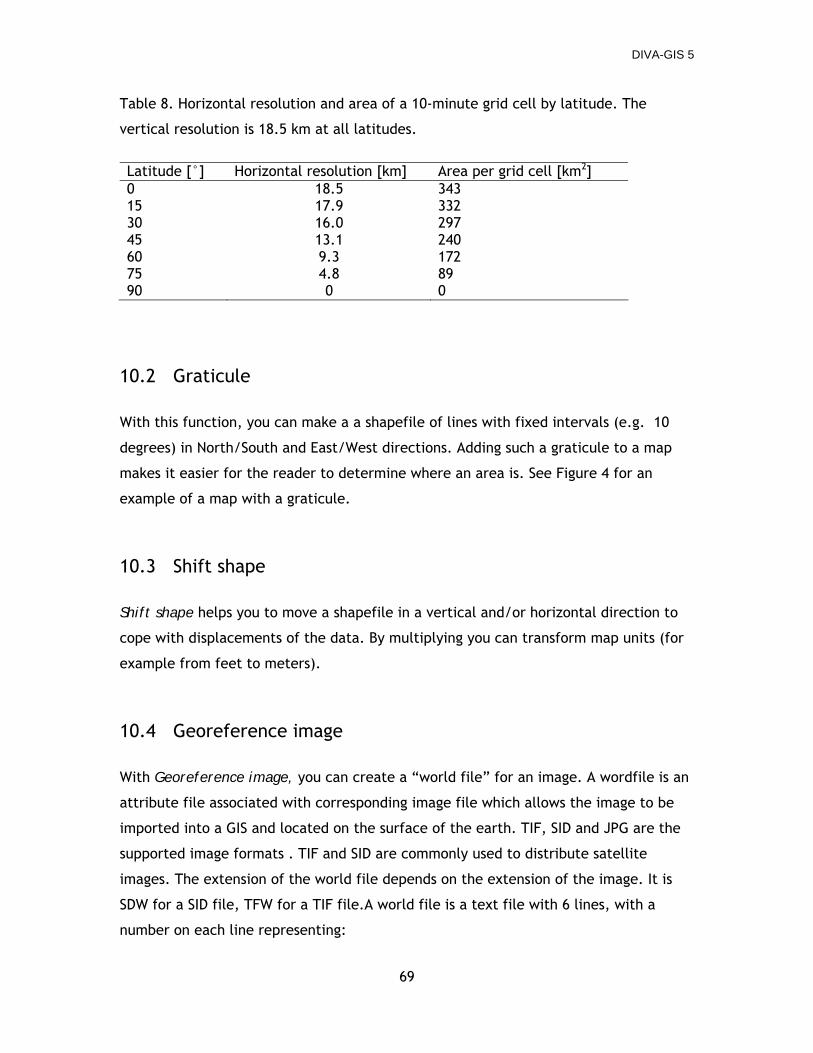
DIVA-GIS 5
69
Table 8. Horizontal resolution and area of a 10-minute grid cell by latitude. The
vertical resolution is 18.5 km at all latitudes.
Latitude [°] Horizontal resolution [km] Area per grid cell [km2] 0 18.5 343 15 17.9 332 30 16.0 297 45 13.1 240 60 9.3 172 75 4.8 89 90 0 0
10.2 Graticule
With this function, you can make a a shapefile of lines with fixed intervals (e.g. 10
degrees) in North/South and East/West directions. Adding such a graticule to a map
makes it easier for the reader to determine where an area is. See Figure 4 for an
example of a map with a graticule.
10.3 Shift shape
Shift shape helps you to move a shapefile in a vertical and/or horizontal direction to
cope with displacements of the data. By multiplying you can transform map units (for
example from feet to meters).
10.4 Georeference image
With Georeference image, you can create a “world file” for an image. A wordfile is an
attribute file associated with corresponding image file which allows the image to be
imported into a GIS and located on the surface of the earth. TIF, SID and JPG are the
supported image formats . TIF and SID are commonly used to distribute satellite
images. The extension of the world file depends on the extension of the image. It is
SDW for a SID file, TFW for a TIF file.A world file is a text file with 6 lines, with a
number on each line representing:
DIVA-GIS 5
70
1. size of pixel in x direction 2. rotation term for row 3. rotation term for column 4. size of pixel in y direction 5. x coordinate of centre of upper left pixel in map units 6. y coordinate of centre of upper left pixel in map units
For example:
28.50 0 0 -28.50 174505.50 2769288.00
Some SID images do not need a world file. In many cases, these images already have
world files (e.g. the SID images that can be downloaded from
https://zulu.ssc.nasa.gov/mrsid/). If your image does not have a world file, you will
need to create one, and you can use the Georeference image tool for that. You will
need to know how many rows and columns your image has. You can find this out with
most graphics programs. You then fill this in, as well as the estimated coordinates of
the extremes of the image. By overlaying a shapefile of the same area, you can see if
the coordinates are correct. You will probably need to change them little by little a
number of times before the image is correctly located.
10.5 Geo-calculator
With the Geo-calculator you can convert coordinates in the sexagesimal (degrees,
minutes, seconds) system to a decimal system. This can be done for one location or for
a file with many locations (use the Batch option). You can also calculate the distance
between two points.
DIVA-GIS 5
71
10.6 General options
The General options window lets you define a number of default settings, including
the font used and the default directories. You can set the default directories where
DIVA-GIS looks for project files and shapefiles, and stores output files.
On the second tab you can specify where DIVA should look for climate (.CLM) files, and
you can inspect and edit the metadata associated with these files.
DIVA-GIS 5
72
REFERENCES
Bonham-Carter, G., 1994. Geographic information systems for geoscientists. Modelling with
GIS. Computer Methods in the Geosciences 13. Pergamon/Elsevier, London, U.K.
Burnham, K.P., and Overton, W.S. 1978. Estimation of the size of a closed population when
capture probabilities vary among animals. Biometrika 65, 623-633.
Busby, J.R. (1991). BIOCLIM - a bioclimatic analysis and prediction system. Pp. 64-68 in
Margules, C.R. and Austin, M.P. (eds) Nature Conservation: Cost Effective Biological
Surveys and data Analysis. Melbourne: CSIRO
Carpenter, G., Gillison, A.N. and Winter, J. 1993. DOMAIN: a flexible modelling procedure for
mapping potential distributions of plants and animals. Biodiversity and Conservation 2:
667-680.
Chao, A., 1984. Non-parametric estimation of the number of classes in a population.
Scandinavian Journal of Statistics 11, 265-270.
Chao, A., 1987. Estimating the population size for capture-recapture data with unequal
catchability. Biometrics 43, 783-791.
Colwell, R. K., and J. A. Coddington. 1994. Estimating terrestrial biodiversity through
extrapolation. Philosophical Transactions of the Royal Society (Series B) 345:101-118.
Cressie, N. A. C., 1991. Statistics for spatial data. John Wiley & Sons, New York.
Greene, S.L. and T. Hart, 1996. Plant Genetic Resource Collections: an Opportunity for the
Evolution of Global Data Sets. Third International Conference/Workshop on Integrating
GIS and Environmental Modeling Santa Fe, New Mexico, USA. (CD-ROM and web
publication; http://www.ncgia.ucsb.edu/conf/SANTA_FE_CD-
ROM/sf_papers/greene_stephanie/sgreene.html).
Heltshe, J. and N.E. Forrester, 1983 . Estimating species richness using the jackknife
procedure. Biometrics 39, 1-11.
Hijmans, R.J., M. Schreuder, J. De la Cruz, and L. Guarino. 1999. Using GIS to check
coordinates of genebank accessions. Genetic Resources and Crop Evolution 46: 291-296.
Hurlbert, S.H., 1978. The non-concept of species diversity: a critique and alternative
parameters. Ecology 52: 577-586.
Intergovernmental Panel on Climate Change Data Distribution Center (1999). Providing climate
change and related scenarios for impact assessment. CD-ROM. Version 1.0. Climate
Research Unit, University of East Anglia, Norwich, UK.
Magurran, A.E. 1988. Ecological diversity and its measurement. Princeton University Press.
Nabhan, G.P. 1990. Wild Phaseolus ecogeography in the Sierra Madre Occidental, Mexico:
aeorographic techniques for targeting and conserving species diversity. Systematic and
DIVA-GIS 5
73
ecogeographic studies on crop genepools 5. International Board for Plant Genetic
Resources, Rome, Italy.
Nelson, A., G. LeClerc and M. Grum, 1997. The development of an integrated Tcl/Tk and C
interface to determine, visualise and interogate infraspecifc bio-diversity. Internal CIAT
document. GIS Laboratory, CIAT, Cali, Colombia.
Nix, H. A. 1986. A biogeographic analysis of Australian elapid snakes. Pp. 415 in R. Longmore
(ed.). Atlas of Elapid Snakes of Australia. Australian Flora and Fauna Series No. 7.
Australian Government Publishing Service, Canberra;
Raaijmakers, J. G. W. 1987. Statistical analysis of the Michaelis-Menten equation. Biometrics
43:793-803.
Rebelo, A.G. 1994. Iterative selection procedures: centres of endemism and optimal placement
of reserves. Strelitzia 1: 231-257
Rebelo, A.G. and W.R. Sigfried. 1992. Where should nature reserves be located in the Cape
Floristic Region, South Africa? Models for the spatial configuration of a reserve network
aimed at maximizing the protection of diversity. Conservation Biology 6:243-252.
Sawada, M., 1999. Rookcase: an Excel 97/2000 Visual Basic (VB) add-in for exploring global and
local spatial autocorrelation. Bulletin of the Ecological Society of America, October 1999:
231-243.
Sanders, H.L., 1968. Marine benthic diversity: a comparative study. American Naturalist
102:243-282.
Smith, E.P. and G. van Belle, 1984. Nonparametric estimation of species richness. Biometrics
40, 119-129.
Wieczorek, J., Q. Guo, and R.J. Hijmans, 2004. The point-radius method for georeferencing
point localities and calculating associated uncertainty. International Journal of
Geographic Information Science 18: 745-767.