Diurnal variation of midlatitudinal ... - atmos-chem-phys.net · Atmos. Chem. Phys., 11, 963–978, 2011 ... tion near full moon with a grating spectrometer. The NO3 column retrieval

Atmos. Chem. Phys., 11, 963–978, 2011www.atmos-chem-phys.net/11/963/2011/doi:10.5194/acp-11-963-2011© Author(s) 2011. CC Attribution 3.0 License.

AtmosphericChemistry

and Physics

Diurnal variation of midlatitudinal NO 3 column abundance overtable mountain facility, California

C. M. Chen1,*, R. P. Cageao1,** , L. Lawrence2,*** , J. Stutz2, R. J. Salawitch1,**** , L. Jourdain1,***** , Q. Li1,2, andS. P. Sander1

1Jet Propulsion Laboratory, California Institute of Technology, Pasadena, California, USA2University of California, Los Angeles, California, USA* now at: Potsdam Institute for Climate Impact Research, Potsdam, Germany** now at: NASA Langley Research Center, Hampton, Virginia, USA*** now at: California Air Resources Board, Sacramento, California, USA**** now at: University of Maryland, College Park, Maryland, USA***** now at: Laboratoire de Physique et Chimie de l’Environnement et de l’Espace, Universite d’Orleans/CNRS, France

Received: 22 June 2010 – Published in Atmos. Chem. Phys. Discuss.: 26 August 2010Revised: 19 January 2011 – Accepted: 27 January 2011 – Published: 2 February 2011

Abstract. The column abundance of NO3 was measuredover Table Mountain Facility, CA (34.4◦N, 117.7◦W) fromMay 2003 through September 2004, using lunar occulta-tion near full moon with a grating spectrometer. The NO3column retrieval was performed with the differential opti-cal absorption spectroscopy (DOAS) technique using boththe 623 and 662 nm NO3 absorption bands. Other spec-tral features such as Fraunhofer lines and absorption fromwater vapor and oxygen were removed using solar spec-tra obtained at different airmass factors. We observed aseasonal variation, with nocturnally averaged NO3 columnsbetween 5− 7× 1013 molec cm−2 during October throughMarch, and 5−22×1013 molec cm−2 during April throughSeptember. A subset of the data, with diurnal variabilityvastly different from the temporal profile obtained from one-dimensional stratospheric model calculations, clearly hasboundary layer contributions; this was confirmed by simul-taneous long-path DOAS measurements. However, eventhe NO3 columns that did follow the modeled time evolu-tion were often much larger than modeled stratospheric par-tial columns constrained by realistic temperatures and ozoneconcentrations. This discrepancy is attributed to substantialtropospheric NO3 in the free troposphere, which may havethe same time dependence as stratospheric NO3.

Correspondence to:C. M. Chen([email protected])

1 Introduction

NO3 plays a significant role in the nocturnal chemistry ofthe stratosphere and troposphere. In the stratosphere, it influ-ences the partitioning of active nitrogen species NO and NO2(NOx), where NOx is an important component in catalyticozone loss cycles. The primary source of NO3 is a reactionbetween NO2 and O3 (ReactionR1), and it is consumed byan additional reaction with NO2 to form the reservoir speciesN2O5 (ReactionR2).

NO2+O3→NO3+O2. (R1)

NO3+NO2+M N2O5+M. (R2)

So as shown in Reaction (R2), NO2, NO3, and N2O5 are inequilibrium. The subsequent removal of N2O5 via a hetero-geneous reaction with water on the surfaces of ice particlesto form nitric acid, also a reservoir species for NOx but withlonger lifetime, contributes to NOx removal. The thermaldecomposition of N2O5 is an additional significant source ofNO3 in the upper stratosphere. Since NO3 photodissociatesextremely rapidly at wavelengths less than about 640 nm, weobserve significant concentrations only at night.

In the troposphere the same formation and destruction re-actions occur with heterogeneous loss of N2O5 occurring onany moist aerosol surface. There is also negligible NO3 dur-ing sunlit hours except for extremely polluted urban settings(Geyer et al., 2003). In the boundary layer, NO3 additionallyis an important nighttime oxidant because it reacts rapidlywith many biogenic hydrocarbons such as alkenes, aldehy-des and terpenes (Atkinson, 1991; Wayne et al., 1991).

Published by Copernicus Publications on behalf of the European Geosciences Union.

http://creativecommons.org/licenses/by/3.0/

964 C. M. Chen et al.: Diurnal variation of midlatitudinal NO3 column abundance

Interest in the role played by NO3 in atmospheric chem-istry increased significantly following the first reports of itsdetection in the stratosphere and troposphere byNoxon etal. (1978, 1980) and Platt et al.(1980). Since then, othermeasurements of atmospheric NO3 column at low and mid-latitudes at urban-influenced and remote ground-based siteshave been made by using the Moon as a light source and em-ploying differential optical absorption spectroscopy (DOAS)(Aliwell and Jones, 1996a,b, 1998; Lal et al., 1993; Renardet al., 2001; Solomon et al., 1989). Also, vertical concentra-tion profiles of NO3 have been inferred from ground-basedmeasurements by observing NO3 in the slant column duringsunrise with direct lunar, zenith sky, and off-axis methods(Allan et al., 2002; Coe et al., 2002; Smith and Solomon,1990; Smith et al., 1993; von Friedeburg et al., 2002; Weaveret al., 1996). As the solar terminator sweeps from the up-per atmosphere down to the surface, photolysis progres-sively decreases the column of NO3, leaving only the col-umn that lies below the terminator altitude. Additionally,stratospheric profiles of NO3 have been obtained from theSAGE III (Stratospheric Aerosol and Gas Experiment) andSCIAMACHY (SCanning Imaging Absorption spectroMe-ter for Atmospheric CartograpHY)Amekudzi et al., 2005)satellite instruments using lunar occultation, and the GO-MOS (Global Ozone Monitoring by Occultation of Stars)(Hauchecorne et al., 2005; Marchand et al., 2004) satelliteinstrument using stellar occultation.

A number of measurements have confirmed the roleof NO3–N2O5 chemistry in the nocturnal boundary layer(Aldener et al., 2006; Allan et al., 2000; Ambrose et al.,2007; Ayers and Simpson, 2006; Brown et al., 2003, 2004;Carslaw et al., 1997a; Geyer et al., 2001; Geyer and Platt,2002; Li et al., 2008; Matsumoto et al., 2006; Mihelcic et al.,1993; Nakayama et al., 2008; Penkett et al., 2007; Platt etal., 1981; Smith et al., 1995; Stutz et al., 2004; Vrekoussis etal., 2007; Wang et al., 2006). Fewer have probed above theboundary layer, essentially those using LP-DOAS (Carslawet al., 1997b), aircraft measurements (Brown et al., 2007a,b)and zenith sky measurements at sunrise (Allan et al., 2002;Coe et al., 2002; von Friedeburg et al., 2002). Due to thisrelative lack of measurements above the boundary layer, therole of NO3–N2O5 chemistry in the free and upper tropo-sphere has not been quantitatively tested.

Our focus is on the quantification of NO3 in the free tro-posphere. We deduce time-resolved estimates of free tro-pospheric NO3 using measurements of total column NO3,observations of the boundary layer concentration of NO3,with stratospheric columns provided by a model. Specifi-cally, we present results of simultaneous measurements ofNO3 column by lunar occultation with the DOAS technique,and surface concentration of NO3 using LP-DOAS, taken onevenings near full moon in August and September 2004 overTable Mountain Facility (TMF), California. Using a clima-tology for ozone concentration and temperature constructedfrom over 10 years of lidar measurements at our measure-

ment site, we get stratospheric partial columns from a strato-spheric model shown to be consistent with SAGE III satellitelunar occultation measurements of NO3. We also used globalchemistry and transport model GEOS-Chem to characterizethe time evolution and vertical distribution of NO3 in thetroposphere for various locations. The full dataset of NO3column measurements was taken from May 2003 throughSeptember 2004, and we characterized the magnitude andvariability of column NO3 at TMF.

2 Experiment description

2.1 Location and measurement frequency

We have acquired direct lunar occultation measurements ofthe NO3 column at Table Mountain Facility (TMF), Califor-nia (34.4◦ N, 117.7◦W) at an altitude of 2280 m. TMF is inthe San Gabriel Mountains north of the Los Angeles Basinand south of the Mojave Desert; therefore it is influenced byclean and polluted air masses. Optimal measurements wereacquired within the 5 day period centered on full moon. Fullmoon conditions offer the longest period of moonlit eveninghours and the highest signal to noise due to the intensity ofreflected sunlight with lunar phase angle opposition effect(Hapke et al., 1993). Observations from May 2003 throughSeptember 2004 consisted of three evenings for each fullmoon event, weather permitting. Measurements during 16out of 18 full moon events were made, resulting in 40 daysof data, out of a possible 90 days.

2.2 Lunar occultation measurement

2.2.1 Instrument configuration

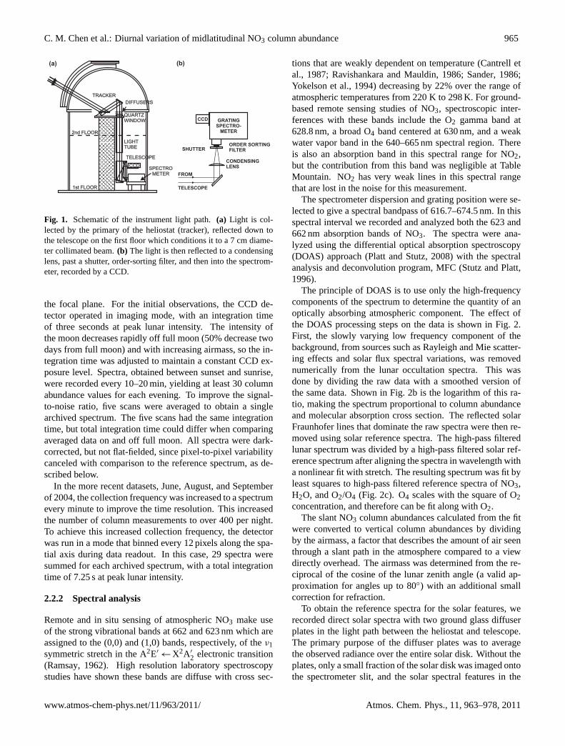
The experimental apparatus (Cageao et al., 2001) is shownin Fig. 1. Light was collected by a heliostat and directed intoan off-axis telescope with 3× magnification. The 7-cm di-ameter collimated beam from the telescope was transmittedthrough a condensing lens, a shutter and order sorting filter(Schott GG-400 glass) to a 0.3 m focal length, f/4 imagingspectrometer (Acton 300i) with a 1200 g mm−1 blazed grat-ing. A slit width of 150 µm was used, resulting in 0.4 nm(FWHM) spectral resolution. The measured spectral rangewas 616.7–674.5 nm. Wavelength calibration for the spec-trometer was obtained by observing a neon Penray lampmounted on the inside of the observatory dome. The shapeand line width of these emission lines also provided the in-strument lineshape function, which was applied to the NO3reference spectra.

The spectrometer was equipped with a 1024×255, back-illuminated CCD detector temperature stabilized with circu-lating coolant. The pixel spacing of the CCD was 26 µm,which resulted in seven times oversampling of the instru-ment line width defined by the entrance slit projected on

Atmos. Chem. Phys., 11, 963–978, 2011 www.atmos-chem-phys.net/11/963/2011/

C. M. Chen et al.: Diurnal variation of midlatitudinal NO3 column abundance 965

TRACKER

QUARTZ

WINDOW

QUARTZ

WINDOW

LIGHT

TUBE

LIGHT

TUBE

2nd FLOOR2nd FLOOR

TELESCOPE

CCDSPECTRO

METER

SPECTRO

METER

1st FLOOR1st FLOOR

DIFFUSERS

ORDER SORTINGFILTERSHUTTER

CONDENSINGLENS

TELESCOPE

GRATINGSPECTRO-

METER

CCD

FROM

(a) (b)

Fig. 1. Schematic of the instrument light path.(a) Light is col-lected by the primary of the heliostat (tracker), reflected down tothe telescope on the first floor which conditions it to a 7 cm diame-ter collimated beam.(b) The light is then reflected to a condensinglens, past a shutter, order-sorting filter, and then into the spectrom-eter, recorded by a CCD.

the focal plane. For the initial observations, the CCD de-tector operated in imaging mode, with an integration timeof three seconds at peak lunar intensity. The intensity ofthe moon decreases rapidly off full moon (50% decrease twodays from full moon) and with increasing airmass, so the in-tegration time was adjusted to maintain a constant CCD ex-posure level. Spectra, obtained between sunset and sunrise,were recorded every 10–20 min, yielding at least 30 columnabundance values for each evening. To improve the signal-to-noise ratio, five scans were averaged to obtain a singlearchived spectrum. The five scans had the same integrationtime, but total integration time could differ when comparingaveraged data on and off full moon. All spectra were dark-corrected, but not flat-fielded, since pixel-to-pixel variabilitycanceled with comparison to the reference spectrum, as de-scribed below.

In the more recent datasets, June, August, and Septemberof 2004, the collection frequency was increased to a spectrumevery minute to improve the time resolution. This increasedthe number of column measurements to over 400 per night.To achieve this increased collection frequency, the detectorwas run in a mode that binned every 12 pixels along the spa-tial axis during data readout. In this case, 29 spectra weresummed for each archived spectrum, with a total integrationtime of 7.25 s at peak lunar intensity.

2.2.2 Spectral analysis

Remote and in situ sensing of atmospheric NO3 make useof the strong vibrational bands at 662 and 623 nm which areassigned to the (0,0) and (1,0) bands, respectively, of theν1symmetric stretch in the A2E′←X2A′2 electronic transition(Ramsay, 1962). High resolution laboratory spectroscopystudies have shown these bands are diffuse with cross sec-

tions that are weakly dependent on temperature (Cantrell etal., 1987; Ravishankara and Mauldin, 1986; Sander, 1986;Yokelson et al., 1994) decreasing by 22% over the range ofatmospheric temperatures from 220 K to 298 K. For ground-based remote sensing studies of NO3, spectroscopic inter-ferences with these bands include the O2 gamma band at628.8 nm, a broad O4 band centered at 630 nm, and a weakwater vapor band in the 640–665 nm spectral region. Thereis also an absorption band in this spectral range for NO2,but the contribution from this band was negligible at TableMountain. NO2 has very weak lines in this spectral rangethat are lost in the noise for this measurement.

The spectrometer dispersion and grating position were se-lected to give a spectral bandpass of 616.7–674.5 nm. In thisspectral interval we recorded and analyzed both the 623 and662 nm absorption bands of NO3. The spectra were ana-lyzed using the differential optical absorption spectroscopy(DOAS) approach (Platt and Stutz, 2008) with the spectralanalysis and deconvolution program, MFC (Stutz and Platt,1996).

The principle of DOAS is to use only the high-frequencycomponents of the spectrum to determine the quantity of anoptically absorbing atmospheric component. The effect ofthe DOAS processing steps on the data is shown in Fig.2.First, the slowly varying low frequency component of thebackground, from sources such as Rayleigh and Mie scatter-ing effects and solar flux spectral variations, was removednumerically from the lunar occultation spectra. This wasdone by dividing the raw data with a smoothed version ofthe same data. Shown in Fig.2b is the logarithm of this ra-tio, making the spectrum proportional to column abundanceand molecular absorption cross section. The reflected solarFraunhofer lines that dominate the raw spectra were then re-moved using solar reference spectra. The high-pass filteredlunar spectrum was divided by a high-pass filtered solar ref-erence spectrum after aligning the spectra in wavelength witha nonlinear fit with stretch. The resulting spectrum was fit byleast squares to high-pass filtered reference spectra of NO3,H2O, and O2/O4 (Fig. 2c). O4 scales with the square of O2concentration, and therefore can be fit along with O2.

The slant NO3 column abundances calculated from the fitwere converted to vertical column abundances by dividingby the airmass, a factor that describes the amount of air seenthrough a slant path in the atmosphere compared to a viewdirectly overhead. The airmass was determined from the re-ciprocal of the cosine of the lunar zenith angle (a valid ap-proximation for angles up to 80◦) with an additional smallcorrection for refraction.

To obtain the reference spectra for the solar features, werecorded direct solar spectra with two ground glass diffuserplates in the light path between the heliostat and telescope.The primary purpose of the diffuser plates was to averagethe observed radiance over the entire solar disk. Without theplates, only a small fraction of the solar disk was imaged ontothe spectrometer slit, and the solar spectral features in the

www.atmos-chem-phys.net/11/963/2011/ Atmos. Chem. Phys., 11, 963–978, 2011


87654ra

w c

ount

s (1

06 )

670660650640630620Wavelength (nm)

-0.3-0.2-0.10.00.1

abso

rban

ce

-50

abs

orba

nce

(10-3

)

-50

-50

-50

-50

NO3

H2O

O2/O4

residual

fits

(a)

(b)

(c)

raw spectrum

high-pass filtered

differential spectrum

Fig. 2. Spectra at different stages of processing:(a) raw spectrum,with visibly sloping baseline,(b) high-pass filtered raw spectrum,created by dividing the raw spectrum with a smoothed version, and(c) the differential spectrum, after subtracting the solar referencespectrum (similar to(b) ), with the individual fits for NO3, water,O2/O4, and the resultant residual. The residual features result fromerrors in fitting the solar line.

non-diffuse spectra differed from those in the lunar spectra.With the diffuser plates, we regularly obtained RMS residualabsorbances of less than 4×10−4. The diffuser plates alsohelped to attenuate the solar beam, although additional neu-tral density filtering was used to avoid detector saturation.

Solar reference spectra were acquired over a day for theairmass range 1–7 (SZA 34–81◦). New solar reference spec-tra were taken once a month during the time of the full moondatasets to account for small changes in instrument align-ment. In addition to solar lines, these spectra contained ter-restrial water vapor, O2, and O4 features with optical depthsthat were proportional to the airmass. The solar reference

spectrum used in the processing for a particular lunar spec-trum had an airmass within±0.5 of the airmass of the lunardata, thereby removing much of the water, O2, and O4 col-umn prior to additional processing. This intrinsically dealswith saturation effects in the water vapor and oxygen spec-tra and provides an accurate representation of the spectrabroaden by instrument line shape. In our experience, usingwater spectra from line-by-line radiative transfer models didnot give the best residuals. Therefore to account for the re-maining and variable water vapor and oxygen signals, weemployed empirical reference spectra obtained from ratiosof solar spectra at different airmasses. Since there is littleoverlap of the O2/O4 and water features, these two featureswere individually isolated and used as empirical spectral ref-erences. The low spectral resolution of measurement doesnot resolve individual lines for water and O2, and thereforehas little sensitivity to pressure broadening. The NO3 refer-ence spectra used were obtained from laboratory absorptioncross section studies of NO3 and have been measured overthe temperature range relevant to the troposphere and strato-sphere (Cantrell et al., 1987; Ravishankara and Mauldin,1986; Ravishankara and Wine, 1983; Sander, 1986; Yokel-son et al., 1994). The cross sections ofSanderandYokel-son et al.are in excellent agreement over the range of over-lap of temperature. Both studies observed a significant de-crease in NO3 cross sections at the peaks of the 662 and623 nm bands with decreasing temperature. In contrast, theresults ofCantrell et al.showed no dependence of cross sec-tion with temperature and are assumed to be incorrect. Theresults ofRavishankara and Mauldindisagree significantlywith those ofYokelson et al.from the same group, and areassumed to be superseded by the latter. Although the tem-perature at the peak of the stratospheric NO3 concentrationprofile at 40 km is roughly 260 K, the average temperatureweighted by the model-predicted NO3 concentration profilein the stratosphere is closer to 240 K. We have used the spec-trum of Yokelson et al. at 240 K for the column retrievalspresented here.Solomon et al.also used a reference temper-ature of 240 K, whileAliwell and Jonesused 260 K.

2.2.3 Measurement uncertainty

The overall uncertainty for our measurement of total columnNO3 is approximately 17% RMS. The most important con-tributions to this uncertainty are systematic errors in crosssection, and photon noise. The stated uncertainty in the NO3cross section is±10% (Yokelson et al., 1994), excludingthe errors associated with the temperature dependence of thecross sections. Our estimate of total column NO3 assumesthat the absorption is dominated by stratospheric contribu-tions. There is a±6% error associated with the use of a sin-gle cross section at a temperature of 240 K, if the temperatureof the column actually varies between 220 K and 260 K. Ifthere are contributions from tropospheric NO3, the retrievedcolumns are a lower limit since the cross section of the band



peak at 662 nm for 298 K is 17% less than for 240 K. Photonnoise in the system contributes an estimated 13% to the un-certainty. The detection limit for the NO3 slant column abun-dance is 2×1012 molec cm−2. The signal to noise ratio was>5 for most of the evening (during the steady state growthperiod); this ratio was larger for measurements through largerairmasses or larger NO3 column amounts.

2.3 Long-path DOAS instrument

Horizontal column average measurements were made atTMF for August and September 2004 using a long-path dif-ferential optical absorption spectrometer (LP-DOAS). LP-DOAS is an active remote sensing technique that givesexceptionally low detection limits by averaging over along (several kilometers) pathlength. Light from a broad-spectrum 500 W Xe arc lamp was collimated through a New-tonian telescope and broadcast to an array of corner-cuberetroreflectors mounted on a radio tower located on the BlueRidge in the Angeles National Forest. The distance betweenthe instrument and the retroreflector array was approximately3.4 km. Light incident on the retroreflector array traveledback through the atmosphere, was collected by the same tele-scope and transmitted through a fiber-optic cable to the spec-trometer and detector. The difference in altitude between theLP-DOAS instrument and the tower-mounted retroreflectorarray was 298 m. A detailed description of the LP-DOASinstrument and the NO3 analysis employed here is given in(Geyer et al., 1999). The measurement uncertainty of theLP-DOAS is dominated by the error in the absorption cross-section of NO3, which is±10% (Yokelson et al., 1994) aspreviously noted.

3 Model descriptions

3.1 1-D stratospheric model

A one-dimensional, photochemical steady state model of thestratosphere (Osterman et al., 1997) was run using TMF cli-matological profiles of temperature and O3 as inputs, andthe modeled NO3 column abundances were compared to theTMF column measurements. The model calculates diur-nally varying species concentrations, assuming each speciesreaches a balance between production and loss over 24 h fora given temperature and pressure profile and latitude. JPL2006 cross sections and quantum yields were used to de-termine photolysis J-values, and JPL 2006 kinetic rate con-stants were used for reaction rates (Sander et al., 2006, 2003).Chemical inputs are profiles of O3, H2O, CH4, NOy, Cly,CO, H2, C2H6, Bry, and aerosol parameters based on a cli-matology derived from NASA satellite and balloon observa-tions (e.g.,Yang et al., 2006), as detailed in Table1.

Additionally, SAGE III satellite measurements of O3 inthe stratosphere were used to verify the consistency betweenthe 1-D stratospheric model and SAGE III measurements of

NO3, testing the current understanding of stratospheric NO3chemistry (described in AppendixA). Analysis of the sen-sitivity of modeled NO3 column to input parameters and touncertainties of reaction rates were also conducted and aredescribed in AppendixB.

3.1.1 Table mountain facility lidar climatology

Temperature and ozone concentration profiles have beenmeasured at TMF by lidar since 1988 and offer a unique op-portunity to compare our measurements with a model withrealistic constraints. Temperature profiles were measuredbetween 30–80 km and ozone profiles between 15–50 km,both with 300 m vertical resolution since September 1994and with 600 m vertical resolution beforehand. Three caseswere run using these data: climatological monthly meanvalues and variability of ozone concentration and tempera-ture over the 10 year period 1988–1997 (data extracted fromthe published contour plots) (Leblanc and McDermid, 2000;Leblanc et al., 1998), and monthly mean profiles for 2003and for 2004 provided byLeblanc(2005). Temperature andozone profiles are sufficient for estimating the NO3 columnsince NO3 is primarily determined by these two quantities, asverified from a sensitivity study described in AppendixB1.

The change in NO3 column at the extremes of variabilitywas probed by running the model with both temperature andozone variability added or subtracted from the climatologicaltemperature and ozone profiles. The uncertainty in the clima-tological temperature measurements are 0.6 K at the middleof the altitude range, 8 K at 30 km, and<4 K at 80 km. Theuncertainty of the climatological ozone measurements are afew percent at the peak of the ozone, 10–15% at 15 km, andmore than 40% above 45 km. The uncertainty in ozone forthe 2003 and 2004 monthly mean profiles was a minimumat 6% at the ozone peak, increasing in error above and be-low this altitude to 10% at 18 km and 42 km. The uncertaintyin temperature for the 2003 and 2004 monthly mean profilesvaried between 0.5 K and 1.3 K over 13–60 km.

The gaps in the ozone and temperature profiles werefilled with the climatology from (1) the Upper AtmosphereResearch Satellite (UARS) Reference Atmosphere Project(URAP) (Remedios et al., 2007; Wang et al., 1999; Ran-del et al., 1999), and then (2) a climatology dataset basedon ozone data fromDutsch(1974) and ozone and tempera-ture from the Middle Atmosphere Program (Barnett and Cor-ney, 1985; Keating and Young, 1985), with adjustments tothe ozone climatology based on in situ ozone measurementsin the upper troposphere and lower stratosphere from manyfield programs. URAP is a compilation of global data fromthe CLAES, HALOE, HRDI, MLS and ISAMS instrumentson the UARS satellite taken from April 1992 through sevenyears, processed into zonal monthly means with standard de-viation. Two types of data were provided: “baseline” dataobtained from April 1992 to March 1993, and “extended”datasets averaged over 7 years. We used extended data where



Table 1. Sources for the input parameters for each of the cases run on the 1-D stratospheric model.

Input parameter Model run

TMF SAGE III sensitivity

temperature TMF lidar data From Sage IIINO3 retrieval

URAP baselinedataset

O3 TMF lidar data From Sage IIINO3 retrieval

URAP extendeddataset

H2O URAP, extended dataset

CH4 URAP, extended dataset

NOy Calculated from tracer relationRinsland et al.(1999);Popp et al.(2001) using URAP N2O baseline dataset

Cly Calculated from tracer relation from SOLVE data, usingURAP N2O baseline dataset

CO Static profile from MkIV flightToon (1991); Sen et al.(1998)

H2 Static profile based on measurementsDessler et al.(1994); Abbas et al.(1996); Rockmann et al.(2003)

C2H6 Static profile from MkIV flight Toon (1991); Sen et al.(1998)

Bry Calculated from tracer relation (Wamsley et al.(1998) us-ing URAP N2O baseline dataset

aerosol parameters Monthly profiles from SAGE II aerosol measurements av-eraged over all years except those affected by the PinatuboeruptionThomason et al.(1997)

a Gaps filled first with URAP dataRemedios et al.(2007); Wang et al.(1999); Randel et al.(1999). For ozone, further gaps were filled by a climatology based onDutsch(1974),on the Middle Atmosphere ProjectKeating and Young(1985), and from many in situ ozone measurements in the lower stratosphere and upper troposphere. For temperature, furthergaps were filled from the Middle Atmosphere ProjectBarnett and Corney(1985).b URAP data is available averaged over 7 years (extended) or over 1992–1993 (baseline).

available. The ozone data used were from the extended timerange, and the temperature data from the baseline time frame.We also used profiles of H2O (extended), CH4 (extended),and N2O (baseline) from URAP. N2O was used as a tracerto estimate model inputs for NOy, Cly, and Bry using wellestablished tracer relations (e.g.Yang et al.(2006) and refer-ences therein).

Static profiles for CO and C2H6 from MkIV measurements(Toon, 1991; Sen et al., 1998), and a H2 profile based onmeasurements in the stratosphere (Abbas et al., 1996; Dessleret al., 1994; Rockmann et al., 2003) were used for all months.Vertical profiles of sulfate aerosol surface area were based onzonal monthly mean measurements by SAGE II (Thomasonet al., 1997) updated to include data acquired during the timeof our NO3 measurements.

3.2 GEOS-Chem tropospheric model

We use the GEOS-Chem global 3-D tropospheric chemistryand transport model (Bey et al., 2001; Park et al., 2004; Wuet al., 2007) to explore the spatial and temporal variability ofNO3 in the troposphere for a few days in August and Septem-ber 2004, coinciding with our acquisition dates. The GEOS-Chem model (version 7.02.04,http://www-as.harvard.edu/chemistry/trop/geos) is driven by the assimilated meteoro-logical GEOS-4 data from NASA Global Modeling and As-similation Office (GMAO) with 6-hour temporal resolution(3-hour for surface variables and mixing depths) and a hor-izontal resolution of 1◦×1.25◦ with 55 layers in the verti-cal. The horizontal resolution of the GEOS-4 wind fields hasbeen degraded to 2◦×2.5◦ for input into GEOS-Chem.


http://www-as.harvard.edu/chemistry/trop/geos

http://www-as.harvard.edu/chemistry/trop/geos


1210

86420(x

1013

mol

ec/c

m2 )

20:00 00:00 04:00 08:00Local Time

34323028262422201816141210

86420

NO3 c

olum

n (x

1013

mol

ec/c

m2 )

(a) August 2004

(b) September 2004

Fig. 3. Diurnal variation of NO3 vertical column measured at Ta-ble Mountain, California for August and September 2004, alongwith calculated vertical columns from the 1-D stratospheric model(line). For August 2004(a), three consecutive evenings of mea-surements are shown, the evenings of 28 August 2004 (open circle),29 August 2004 (+), and 30 August 2004 (filled diamond). Alsofor September 2004(b), three consecutive evenings of measure-ments are shown the evenings of 27 September 2004 (open circle),28 September 2004 (+), and 29 September 2004 (filled diamond).The stratospheric model used monthly mean profiles from TMF li-dar measurements from 2004 as input. Data from September, dur-ing the steady state nocturnal period, shows only every tenth pointto avoid crowding the graph.

4 Results and discussion

4.1 Experimental results

As seen in model calculations in Fig.3, the diurnal variationof stratospheric NO3 can be characterized by four phases:daytime photolysis (negligible NO3), sunset build-up (a rapidrise in NO3 column), nocturnal steady state (a nearly lin-ear, slow rise in NO3 column), and sunrise destruction (rapiddecrease in NO3 column). These four stages were also ob-served in our measurements, except for some variations dur-ing the nocturnal steady state stage. Time series that mono-tonically increase, which occurs almost linearly during thesteady state phase, are labeled as “model-like behavior” asseen in our measurements from September 2004 (Fig.3b);

28262422201816141210

86420

NO3 c

olum

n (x

1013

mol

ec/c

m2 )

360300240180120600day of the year

J F M A M J J A S O N D

Fig. 4. Table Mountain Facility (TMF) NO3 vertical column mea-surements compared to results from the 1-D photochemical modelusing TMF lidar profiles of ozone and temperature as inputs, plot-ted vs. day of year. Both the measured and modeled columns wereaveraged over the steady state portion of the night. The measuredmean NO3 columns shown are from 2003 (triangles)–2004 (cir-cles); model-like and non-modeled behavior are denoted by openand filled symbols, respectively. The bars show the diurnal vari-ability. The three cases run by the model are: the climatology from1988–1997 along with the limits of the temperature and ozone vari-ability taken fromLeblanc et al.(Leblanc et al., 1998; Leblanc andMcDermid, 2000), and mean profiles fromLeblanc(Leblanc, 2005)for 2003 and 2004.

this label does not necessarily mean that these data are purelystratospheric in origin. The remaining data are described as“non-modeled behavior”, and displayed a wide variety of dif-ferent temporal behavior with variability ranging from oneto several hours, as seen in our measurements from August2004 (Fig.3a).

For purposes of comparison, each night of data was re-duced to a time-averaged mean column and a standard devi-ation over the steady state phase, which was taken to be twohours after sunset up to roughly 30 min before sunrise. Anannual plot of all the mean columns, with 2-σ standard devia-tions as error bars, is shown in Fig.4. For 26 of the 40 days ofanalyzed data, the NO3 columns followed model-like behav-ior (open symbols in Fig.4). Within this subset of data a sea-sonal variation was observed, more clearly shown in Fig.5.The NO3 mean column averaged over summer months (Aprilthrough September) was 7.5×1013 molec cm−2. The col-umn averaged over winter months (October through March)was 5.5×1013 molec cm−2, as summarized in Table2;



14

12

10

8

6

4

2

0

NO3 c

olum

n (x

1013

mol

ec/c

m2 )

360300240180120600day of the year

J F M A M J J A S O N D

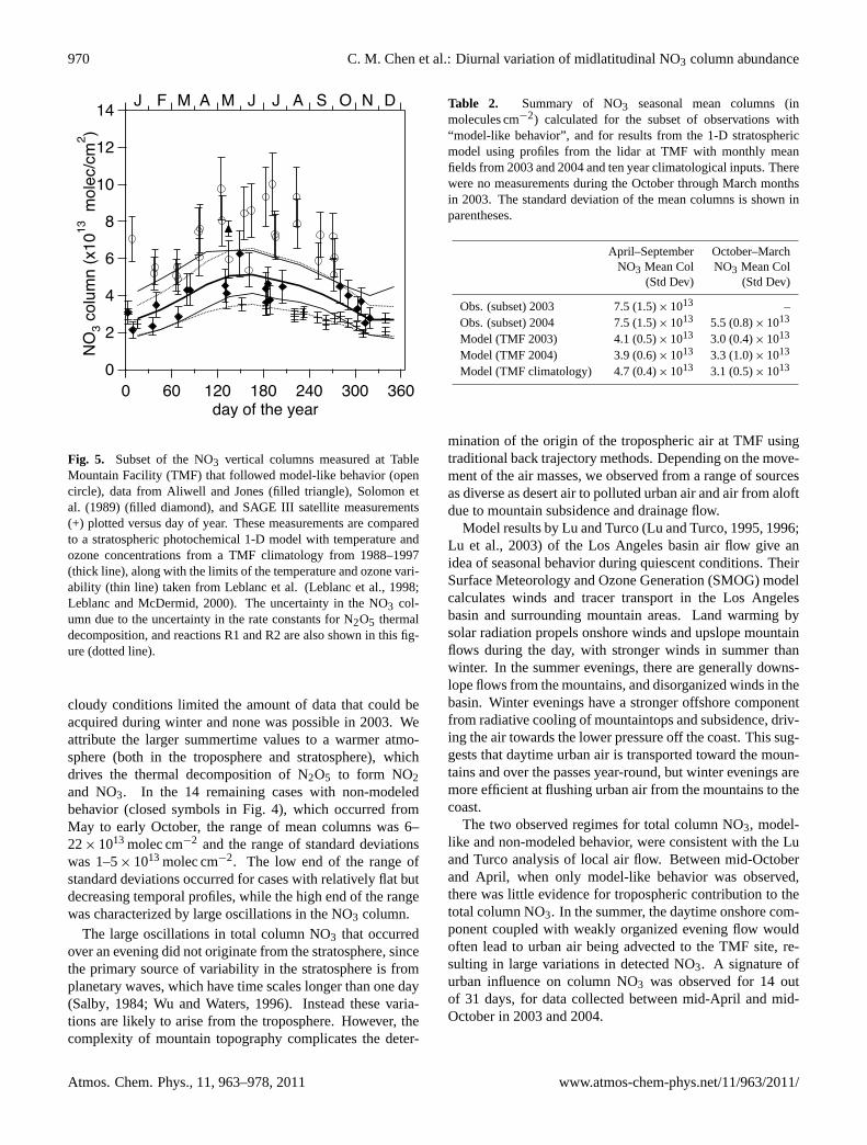
Fig. 5. Subset of the NO3 vertical columns measured at TableMountain Facility (TMF) that followed model-like behavior (opencircle), data from Aliwell and Jones (filled triangle),Solomon etal. (1989) (filled diamond), and SAGE III satellite measurements(+) plotted versus day of year. These measurements are comparedto a stratospheric photochemical 1-D model with temperature andozone concentrations from a TMF climatology from 1988–1997(thick line), along with the limits of the temperature and ozone vari-ability (thin line) taken fromLeblanc et al.(Leblanc et al., 1998;Leblanc and McDermid, 2000). The uncertainty in the NO3 col-umn due to the uncertainty in the rate constants for N2O5 thermaldecomposition, and reactionsR1 andR2 are also shown in this fig-ure (dotted line).

cloudy conditions limited the amount of data that could beacquired during winter and none was possible in 2003. Weattribute the larger summertime values to a warmer atmo-sphere (both in the troposphere and stratosphere), whichdrives the thermal decomposition of N2O5 to form NO2and NO3. In the 14 remaining cases with non-modeledbehavior (closed symbols in Fig.4), which occurred fromMay to early October, the range of mean columns was 6–22×1013 molec cm−2 and the range of standard deviationswas 1–5×1013 molec cm−2. The low end of the range ofstandard deviations occurred for cases with relatively flat butdecreasing temporal profiles, while the high end of the rangewas characterized by large oscillations in the NO3 column.

The large oscillations in total column NO3 that occurredover an evening did not originate from the stratosphere, sincethe primary source of variability in the stratosphere is fromplanetary waves, which have time scales longer than one day(Salby, 1984; Wu and Waters, 1996). Instead these varia-tions are likely to arise from the troposphere. However, thecomplexity of mountain topography complicates the deter-

Table 2. Summary of NO3 seasonal mean columns (inmolecules cm−2) calculated for the subset of observations with“model-like behavior”, and for results from the 1-D stratosphericmodel using profiles from the lidar at TMF with monthly meanfields from 2003 and 2004 and ten year climatological inputs. Therewere no measurements during the October through March monthsin 2003. The standard deviation of the mean columns is shown inparentheses.

April–September October–MarchNO3 Mean Col NO3 Mean Col

(Std Dev) (Std Dev)

Obs. (subset) 2003 7.5 (1.5)×1013 –Obs. (subset) 2004 7.5 (1.5)×1013 5.5 (0.8)×1013

Model (TMF 2003) 4.1 (0.5)×1013 3.0 (0.4)×1013

Model (TMF 2004) 3.9 (0.6)×1013 3.3 (1.0)×1013

Model (TMF climatology) 4.7 (0.4)×1013 3.1 (0.5)×1013

mination of the origin of the tropospheric air at TMF usingtraditional back trajectory methods. Depending on the move-ment of the air masses, we observed from a range of sourcesas diverse as desert air to polluted urban air and air from aloftdue to mountain subsidence and drainage flow.

Model results by Lu and Turco (Lu and Turco, 1995, 1996;Lu et al., 2003) of the Los Angeles basin air flow give anidea of seasonal behavior during quiescent conditions. TheirSurface Meteorology and Ozone Generation (SMOG) modelcalculates winds and tracer transport in the Los Angelesbasin and surrounding mountain areas. Land warming bysolar radiation propels onshore winds and upslope mountainflows during the day, with stronger winds in summer thanwinter. In the summer evenings, there are generally downs-lope flows from the mountains, and disorganized winds in thebasin. Winter evenings have a stronger offshore componentfrom radiative cooling of mountaintops and subsidence, driv-ing the air towards the lower pressure off the coast. This sug-gests that daytime urban air is transported toward the moun-tains and over the passes year-round, but winter evenings aremore efficient at flushing urban air from the mountains to thecoast.

The two observed regimes for total column NO3, model-like and non-modeled behavior, were consistent with the Luand Turco analysis of local air flow. Between mid-Octoberand April, when only model-like behavior was observed,there was little evidence for tropospheric contribution to thetotal column NO3. In the summer, the daytime onshore com-ponent coupled with weakly organized evening flow wouldoften lead to urban air being advected to the TMF site, re-sulting in large variations in detected NO3. A signature ofurban influence on column NO3 was observed for 14 outof 31 days, for data collected between mid-April and mid-October in 2003 and 2004.



In Fig. 5, our model-like behavior data are shown com-pared to other measured column measurements using lunaroccultation with grating spectrometers, fromSolomon et al.(1989) andAliwell and Jones(1996b). Data fromSolomonet al. were taken from Fig. 10 of their paper and reduced by18% to account for the updated NO3 cross section ofYokel-son et al.at 240 K, which was not available when the paperwas published. The result ofAliwell and Jonesand our dataare in good agreement. While some of our data and that ofSolomon et al.have overlapping error bars, the majority oftheir data is roughly 1–2×1013 molec cm−2 below the TMFcolumns. Solomon et al.confirmed most of their data wasprimarily stratospheric NO3 by analyzing the dependence ofthe NO3 slant column on the lunar zenith angle (LZA) nearthe horizon (LZA> 80◦) (Solomon et al., 1989). A tropo-spheric NO3 signal would grow much faster than the strato-spheric NO3 at high lunar zenith angles from slant path in-creases. We were not able to use this method to determine thetropospheric contribution because of pointing system viewangles limited to less than 80◦.

Surface concentration measurements of NO3 were madewith the UCLA LP-DOAS instrument during the Augustand September 2004 measurement periods. The results areshown along with the NO3 column amounts measured by lu-nar occultation in Fig.6. As shown in the figure, the shorttime-scale features in the 29–31 August LP-DOAS data arereproduced in the column data, implying a large boundarylayer contribution to the column on those days. Some fea-tures seen in the column measurements were not present inthe surface concentrations, which could be due to changingthickness of the polluted layer.

In contrast, data from 27–29 September 2004 had a muchsmaller contribution from the boundary layer. The LP-DOASinstrument confirmed that there were low NO3 concentra-tions at the surface, as show in Fig.6. This period coincidedwith a Santa Ana wind event, characterized by a northerlydownslope flow that advected dry desert air mixed with airfrom aloft over the measurement site. This circulation isdriven by a high pressure system centered north of SouthernCalifornia. This flow of air from the north over the moun-tains and through the passes to the LA basin drives windspeeds of 46 km h−1 and gusts in excess of 90 km h−1, carry-ing urban pollution offshore and away from Table MountainFacility. Air quality measurements of surface NO2, CO, andO3 from Air Quality Management District (AQMD) stations(California Air Resources Board, 2007) in Victorville (14306Park Avenue), Azusa, downtown Los Angeles (North MainStreet), and west Los Angeles (Westchester Parkway), posi-tioned progressively from the desert in Victorville towardsthe ocean, verifies that low concentrations of surface urbanpollutants were found in the Mojave Desert and into Los An-geles County, and that the diurnal cycle for these chemicalswas disrupted for this time period (see Fig.7).

300

200

100

0NO3 m

ixing

ratio

(ppt

)

12:00 AM8/29/2004

12:00 PM 12:00 AM8/30/2004

12:00 PM 12:00 AM8/31/2004

local time

3.0

2.0

1.0

0.0

NO3 colum

n (x1014 m

olec/cm2)

300

200

100

0NO3 m

ixing

ratio

(ppt

)

12:00 AM9/28/2004

12:00 PM 12:00 AM9/29/2004

12:00 PM 12:00 AM9/30/2004

local time

3.0

2.0

1.0

0.0

NO3 colum

n (x1014 m

olec/cm2)

Fig. 6. Coincident measurements of NO3 vertical column (in red)using lunar occultation and surface measurements of NO3 concen-tration (in black) using long-path DOAS. Many of the large featuresin the data taken in August 2004 occur in both datasets. Measure-ments in September 2004 verify that there were very low levels ofNO3 concentration at the surface the whole evening.

4.2 Model results

4.2.1 Stratospheric model

Model results using averaged TMF temperatures over threedifferent time periods are shown in Fig.4: monthly averagesfrom 2003, from 2004, and over a ten year period, 1988–1997. All three TMF model results exhibited a seasonal vari-ability with higher values during the summer. Results from2003 followed those of the ten-year average, with Novemberthrough January having the lowest values of the year, and thehighest values in April and May. Results from 2004 deviatedfrom the other runs with larger modeled columns for Januarythat decreased to climatological values from March onwards.The TMF seasonal averages for total column NO3 are listedin Table2.

4.2.2 Tropospheric model

From the results of the GEOS-Chem 3-D chemical transportmodel, we investigated the expected range of troposphericNO3 column abundances for specific geographic regions.GEOS-Chem could not be used for quantitative comparisonswith TMF observations since the grid size is too large to re-solve the local meteorology and the detailed transport of pol-lution from the LA Basin. In order to understand the rangeof the expected NO3 variability from the model, columnabundances are compared for three different locations: TMF(mountainous region with nearby urban pollution sources,33–35◦ N, 241.25–243.75◦ E), western Colorado (northernmidlatitude mountain area, 37–41◦ N, 251.25–253.75◦ E),and the northern midlatitude Pacific Ocean (no urban sources



Fig. 7. Time series data for NO2, CO, and O3 mixing ratio (offsetprogressively by 0.05 ppm) at three AQMD monitoring sites locatedin the Mojave Desert and progressively towards Los Angeles: Vic-torville (black dot), Azusa (red dash), and downtown Los Angeles(blue solid). The Santa Ana winds occurred 28–30 September 2004,evidenced by the disturbance of the diurnal cycle and lower diurnalconcentrations. The date labels correspond to 00:00 for each day.

or orographic influences, 29–45◦ N, 178.75–228.75◦ E). Inaddition, we calculate the NO3 column for the northernmidlatitude zonal mean (29–45◦N). The regions were com-pared for six evenings that coincide with data collection (theevenings of 28–30 August 2004 and 27–29 September 2004).Total columns as well as the partial columns from the bound-ary layer and free troposphere were calculated.

The boundary layer defined by the model for each timestep was not used since the boundary layer is shallower dur-ing night time and does not reflect the pollution that was dis-tributed throughout the boundary layer in the daytime. In-stead, a column was constructed by setting the boundary tothe maximum thickness of the boundary layer for that day.This column is labeled as the “thickest boundary layer”, withthe difference of the total with this quantity labeled as the“thinnest free troposphere”.

The time evolution of tropospheric NO3, shown in Fig.8and Fig.A1, varied over the different regions but in mostcases there was a sawtooth pattern not unlike that for thestratosphere: daytime photolysis with negligible NO3, anearly linear rise in NO3 column over the evening followedby a rapid decrease in NO3 column at sunrise. The thick-est boundary layer column tended to mimic the total columnshape, but for all cases the thinnest free tropospheric columnconsistently had the sawtooth pattern.

The diurnal averages, calculated with the same method aswith the measurements, are summarized in Table3. The

Table 3. Mean, median, and standard deviation of column NO3from the GEOS-Chem 3-D global transport and chemistry modelfor the evenings of 28–30 August 2004 and 27–29 September 2004,which coincide with data collection days. Four regions were inves-tigated, Los Angeles (contains TMF), northern midlatitude Pacific,western Colorado, and the northern midlatitude band (30–45◦ N).the columns are calculated as total, the column below the maximumextent of the boundary layer for the previous day, and the columnabove.

NO3 Mean Column (×1013 cm−2)

Los Angeles N midlat Pacific

Total BL∗ FT∗ Total BL∗ FT∗

28 August 2004 71 73 13 5.6 0.018 5.629 August 2004 69 59 10 5.3 0.015 5.330 August 2004 73 64 9.3 5.2 0.015 5.2

27 September 2004 54 48 5.5 4.7 0.033 4.728 September 2004 34 28 5.4 5.0 0.051 5.029 September 2004 16 10 5.7 5.0 0.097 4.9

Western Colorado Northern midlatitude band

Total BL∗ FT∗ Total BL∗ FT∗

28 August 2004 4.3 3.3 1.1 9.6 3.3 6.429 August 2004 5.7 4.7 1.0 9.0 2.9 6.130 August 2004 7.0 6.0 0.95 8.9 2.9 6.0

27 September 2004 4.5 3.5 1.1 9.7 3.8 5.828 September 2004 4.5 2.4 2.1 9.4 3.4 6.029 September 2004 2.9 1.9 0.98 11 3.8 6.8

model grid cell over Los Angeles has large troposphericNO3 columns from anthropogenic NOx with roughly 20–70×1013 molec cm−2, while the data at a midlatitude moun-tainous region (western Colorado) and without nearby ur-ban sources (northern midlatitude Pacific) had significantlysmaller tropospheric columns (4–5×1013 molec cm−2). Thethinnest free tropospheric column was at its lowest over themountain region, (1×1013 molec cm−2). The midlatitudezonal mean value is 6×1013 molec cm−2. These values areconsistent with the difference between our TMF measure-ments of total column NO3 and model amounts of strato-spheric partial column NO3. As discussed below, this sug-gests that NO3 in the free troposphere can regenerate eachevening to substantial concentrations over a series of days,indistinguishable from stratospheric NO3 based solely on thetime evolution (diurnal variation) of the measured signal.This indicates a lack of chemical loss of NOx and a highoxidation capacity in the upper troposphere.

4.3 Model and measurement comparison

The measured NO3 columns along with results from 1-Dstratospheric model constrained by measured temperaturesand ozone concentrations from TMF showed a seasonal trendwith higher NO3 in the summer months. Measurements



Fig. 8. Time evolution of total tropospheric vertical column (black),“thickest boundary layer” vertical column (red), and “thinnest freetropospheric” vertical column (blue) as calculated from 3-D globalchemical transport model GEOS-Chem, for four different regionsduring three days in August. The “thickest boundary layer” col-umn for an evening is the column calculated from the surface tothe height of the maximum thickness boundary layer from the pre-ceding day. The thinnest free troposphere is the difference betweenthe total tropospheric column and the thickest boundary layer. Thefour regions are Los Angeles (33–35◦ N, 241.25–243.75◦ E), west-ern Colorado (37–41◦ N, 251.25–253.75◦ E), the northern midlati-tude Pacific Ocean (29–45◦ N, 178.75–228.75◦ E), and in the north-ern midlatitude band (29–45◦ N).

and model results from January–March 2004 were consistentwithin error bars as seen in Fig.4, even duplicating the de-crease in mean NO3 column over these months not seenin the other model results. However, as seen in Table2,the measured data are consistently larger than the modeleddata by over 2×1013 molec cm−2 for both summer and win-ter averages. This suggests that there is significant NO3in the troposphere; the stratospheric model correlated wellwith measured stratospheric NO3 columns from SAGE III,as discussed in AppendixA, therefore we believe the modelis reliable.

While it is clear that our NO3 columns exhibiting non-modeled behavior have contributions from the boundarylayer, even days with established low surface NO3 concen-trations, such as 27–30 September 2004 (Fig.3b), had meancolumns of NO3 that were on average 2×1013 molec cm−2

more than the model amount. Low levels of NO3 were de-tected by LP-DOAS in September, but the measured columnswere still on average 2×1013 molec cm−2 greater than themodeled column, which is more NO3 than a uniform tro-posphere with 3 ppt of NO3, the detection limit of the in-strument. Other measurements have determined there canbe significantly larger concentrations of NO3 above the sur-face in the upper boundary layer and lower free troposphere,using zenith sky measurements at sunrise compared to sur-

face DOAS measurements (Allan et al., 2002). GEOS-Chemresults for the northern midlatitude band (29–45◦N) for thesix days in August and September 2004 highlighted in thisstudy found that the average thinnest free tropospheric col-umn was 6×1013 molec cm−2 while the average thickestboundary layer column was 3×1013 molec cm−2. For thiscase, significant NO3 existed in the free troposphere withsmoothly varying diurnal variation that is indistinguishablefrom modeled stratospheric NO3 diurnal variation. This re-sult indicates there is a sizable contribution to the column ofNO3 from the troposphere above the boundary layer.Brownet al. (2007a) reached similar conclusions based on aircraftmeasurements over the east coast of the United States.

5 Conclusions

We have measured the diurnal variation of the NO3 col-umn over Table Mountain Facility, California (34.4◦ N,117.7◦W), using ground-based visible absorption spec-troscopy of moonlight. We observed two sets of behaviorduring the steady state phase of the evening: one describedas “model-like behavior” followed the expected slow lin-ear increase (mean columns of 5–9×1013 molec cm−2 for26 out of 40 days), and the other, called “non-modeledbehavior”, showed large departures from model behav-ior, often correlated with large mean NO3 columns (6–22×1013 molec cm−2 over 14 out of 40 days) and large stan-dard deviations (up to 5×1013 molec cm−2), mostly duringMay through early October. The changes in NO3 columnseen in the non-modeled data are not likely due to variabil-ity in the stratosphere and are attributed to boundary layersources.

Comparison to results from a 1-D photochemical modelwith temperature and ozone profiles taken from onsite lidarinstruments showed that for the most part we measured moreNO3 than found using the model. The model compares wellwith stratospheric column NO3 reported by SAGE III. Thesecomparisons suggest significant contributions to total columnNO3 from the free troposphere at all times, with the tropo-spheric contribution exhibiting a diurnal pattern similar to thestratospheric column. This is supported by simultaneous sur-face measurements with LP-DOAS in September 2004, andresults from the global tropospheric chemical and transportmodel, GEOS-Chem. This indicates that the upper tropo-sphere has similar chemical processes and characteristics asthe stratosphere.

Appendix A

The SAGE III (Meteor-3M) instrument (SAGE III ATBD,2002) retrieved NO3 concentration profiles from 20–60 kmand O3 concentration profiles from 15–50 km by satellite lu-nar occultation at moonset or moonrise. The retrieval processused temperature and pressure profiles from meteorological



Fig. A1. Same as Fig.8 except for September.

data from the National Centers for Environmental Prediction(NCEP) (Kalnay et al., 1996). These NCEP temperature andpressure profiles along with the SAGE III retrieved O3 pro-files were used as inputs for the stratospheric model and theresulting modeled NO3 columns were compared with SAGEIII NO3 measurements. Available data spans from May 2002to October 2005 (the mission was terminated March 2006),and 1184 data points from the latitude band between−70and 70◦ were used; local times of the measurements werebetween 22:00–02:00.

The 1-D stratospheric model described in the paper wasrun with inputs from SAGE III lunar O3 measurements aswell as the temperature and pressure data from NCEP reanal-ysis used in the SAGE III retrievals. The O3 profile below15 km and above 50 km was filled with a climatology basedon Dutsch and the Middle Atmosphere Project, described inthe model description in the body of the paper; this has lit-tle impact on the scientific interpretation of our results, sincethe altitude range of interest for NO3 is covered by the SAGEIII measurements. The rest of the chemical inputs were thesame as described for the TMF model runs.

The NO3 profiles were integrated over the 18–60 km alti-tude range to determine a stratospheric partial NO3 columncomparable to the one calculated from SAGE III data. Thesecolumns were further reduced to a mean column and standarddeviation calculated over the nocturnal steady state period, asdone with our measurements.

The modeled stratospheric NO3 columns are plottedagainst the values derived from integration of the SAGEIII NO3 vertical profiles in Fig.A2. The bulk of the datapoints cluster along the one-to-one line. Since both sets ofdata have significant uncertainties, we used a linear fit thatconsidered bothx and y errors (the details are describedin Wang et al., 2008), rather than a standard linear fit thatconsiders only errors iny. The uncertainty in the mod-eled NO3 column due to uncertainties in input temperature

6

5

4

3

2

1

Mod

el c

olum

n (x

1013

mol

ec/c

m2 )

654321SAGE III column (x1013 molec/cm2)

Fig. A2. Modeled NO3 vertical columns using SAGE III lunar pro-files as model input, compared to the SAGE III measured NO3columns within a band from 70◦ S to 70◦ N. The one-to-one l ineis shown as a solid line, and a linear fit to the data (with a slope of0.92) is shown as a dashed line. The uncertainty in the SAGE IIINO3 column (2×1012molec cm2) and the uncertainty in the mod-eled column (7×1012molec cm2) are shown on one data point.

and O3 profiles was estimated to be 0.7×1013 molec cm−2,and uncertainty in the measured NO3 column derived fromthe quoted uncertainties in the SAGE III NO3 retrieved pro-files was 0.2×1013 molec cm−2. This resulted in a lin-ear fit with a slope of 0.92±0.02 and an intercept of0.42×1013 molec cm−2, with a reduced Chi squared,χ2

red,of 4.3. The reduced Chi squared is theχ2 statistic normal-ized by the degrees of freedom, with a value of one indicativeof a good fit (residual of fit and data is same order as errors),much less than one an indication of overestimated errors,and much greater than one of underestimated errors. Fromthese fit results we assert that the modeled stratospheric NO3columns are consistent with the SAGE III measured columns.

Appendix B

B1 Sensitivity study of modeled NO3 on inputparameters in 1-D stratospheric model

We conducted a sensitivity study of the 1-D stratosphericmodel to determine to which input parameters the NO3 col-umn was most sensitive. Changes of±5% concentration or±5 K were applied to the entire vertical profile of an in-dividual input parameter. These changes were applied to



Table B1. Summary of sensitivity coefficients due to variationsin temperature, ozone, and relevant reaction rate constants. Tem-perature was varied by±5 K, ozone by±5%, NOy by ±5%,and the rate constants were varied by their quoted error limits(Sander et al., 2003).

Sensitivity coefficients

Negativevariation

Positivevariation

Temperature (5 K) −0.25 0.36O3 (5%) −0.05 0.05NOy (5%) −0.01 0.01

NO2+O3→NO3+O2 −0.24 0.29N2O5→NO3+NO2 −0.04 0.06NO3+NO2+M↔N2O5+M 0.12 −0.12

atmospheric profiles using the URAP climatology for alltwelve months. Other chemical profiles not provided byURAP used the same sources as described for the TMFmodel runs.

We found that out of the various input parameters to the1-D model, the NO3 column is most sensitive to temperatureand O3. An increase or decrease of temperature by 5 K in themodel resulted in change in the mean NO3 column by 36%or −25%, respectively. A linear response was observed be-low 30 km; from 30–45 km a strongly nonlinear response wasobserved. A change of±5% in the ozone concentration re-sulted in a change in the mean NO3 column by±5%, with noaltitude dependence in the sensitivity from 18–50 km. Thisdirectly proportional, linear relationship between NO3 andozone concentration occurs when NO3 concentration is insteady state. NOy also had a small effect, with the±5%change in NOy concentration resulting in a±1% change inthe NO3 column. The effect on NO3 from changes in the in-put concentration of other chemicals was negligible. Thesesensitivity coefficients are summarized in TableB1.

B2 Error propagation of reaction rates to NO3 columns

Sensitivity of the NO3 column to the errors in the rates ofreactions relevant to NO3 concentration was probed. The re-action rates of NO3 creation from NO2 + O3 (R1), thermaldecomposition of N2O5, and N2O5 formation (R2), were in-dividually changed by their quoted error (Sander et al., 2003)for the SAGE III runs described in the model description,section3.1. The sensitivity coefficients are summarized inTableB1. The greatest sensitivity of the NO3 column to re-action rate errors was found for the NO3 formation reactionfrom NO2 + O3. The root-mean-square variation for all ratechanges that increase NO3 was 27%, and 32% for changesthat decrease NO3 column. These percent changes were ap-

plied to the TMF climatology and are plotted as the pair ofdotted lines in Fig.5. The plotted range of NO3 columns dueto reaction rate errors was of similar magnitude as the rangeof NO3 values calculated from the variability observed by theTMF lidar.

Acknowledgements.The research described in this paper wascarried out at Jet Propulsion Laboratory, California Instituteof Technology. It was supported by grants from the NationalAeronautics and Space Administration. The SAGE III data used inthis comparison are from L2 Lunar Event Species Profiles, v3.00,available from the NASA Langley Research Center AtmosphericSciences Data Center (http://eosweb.larc.nasa.gov). We thankR. Moore for assistance with the SAGE III data, T. Leblanc forthe TMF lidar data, Atmospheric and Environmental Research foruse of LBLRTM, and S. Wang and A. Lambert for the orthogonallinear fit program. We also thank D. Natzic for technical assistance,L. Kovalenko for assistance with the photochemical model, andH. Bosch for discussions and calculations on atmospheric scatter-ing. Others who have made significant technical and discussioncontributions include R. Lu, D. Wu, G. Mount, V. Nemtchinov, andD. Peterson.

Edited by: J. B. Burkholder

References

Abbas, M. M., Gunson, M. R., Newchurch, M. J., Michelsen, H.A., Salawitch, R. J., Allen, M., Abrams, M. C., Chang, A. Y.,Goldman, A., Irion, F. W., Moyer, E. J., Nagaraju, R., Rinsland,C. P., Stiller, G. P., and Zander, R.: The hydrogen budget of thestratosphere inferred from ATMOS measurements of H2O andCH4, Geophys. Res. Lett., 23, 2405–2408, 1996.

Aldener, M., Brown, S. S., Stark, H., Williams, E. J., Lerner, B.M., Kuster, W. C., Goldan, P. D., Quinn, P. K., Bates, T. S.,Fehsenfeld, F. C., and Ravishankara, A. R.: Reactivity and lossmechanisms of NO3 and N2O5 in a polluted marine environ-ment: Results from in situ measurements during New EnglandAir Quality Study 2002, J. Geophys. Res.-Atmos., 111, D23S73,doi:10.1029/2006JD007252, 2006.

Aliwell, S. R. and Jones, R. L.: Measurement of atmospheric NO31. Improved removal of water vapour absorption features in theanalysis for NO3, Geophys. Res. Lett., 23, 2585–2588, 1996a.

Aliwell, S. R. and Jones, R. L.: Measurement of atmospheric NO32, Diurnal variation of stratospheric NO3 at midlatitude, Geo-phys. Res. Lett., 23, 2589–2592, 1996b.

Aliwell, S. R. and Jones, R. L.: Measurements of tropospheric NO3at midlatitude, J. Geophys. Res.-Atmos., 103, 5719–5727, 1998.

Allan, B. J., McFiggans, G., Plane, J. M. C., Coe, H., and Mc-Fadyen, G. G.: The nitrate radical in the remote marine boundarylayer, J. Geophys. Res.-Atmos., 105, 24191–24204, 2000.

Allan, B. J., Plane, J. M. C., Coe, H., and Shillito, J.: Observationsof NO3 concentration profiles in the troposphere, J. Geophys.Res.-Atmos., 107, 4588, doi:10.1029/2002JD002112, 2002.

Ambrose, J. L., Mao, H., Mayne, H. R., Stutz, J., Talbot, R., andSive, B. C.: Nighttime nitrate radical chemistry at Appledoreisland, Maine during the 2004 international consortium for at-mospheric research on transport and transformation, J. Geophys.Res.-Atmos., 112, D21302, doi:10.1029/2007JD008756, 2007.


http://eosweb.larc.nasa.gov


Amekudzi, L. K., Sinnhuber, B. M., Sheode, N. V., Meyer,J., Rozanov, A., Lamsal, L. N., Bovensmann, H., andBurrows, J. P.: Retrieval of stratospheric NO3 verticalprofiles from SCIAMACHY lunar occultation measurementover the Antarctic, J. Geophys. Res.-Atmos., 110, D20304,doi:10.1029/2004JD005748, 2005.

Atkinson, R.: Kinetics and Mechanisms of the Gas-Phase Reactionsof the NO3 Radical with Organic-Compounds, J. Phys. Chem.Ref. Data, 20, 459–507, 1991.

Ayers, J. D. and Simpson, W. R.: Measurements of N2O5 nearFairbanks, Alaska, J. Geophys. Res.-Atmos., 111, D14309,doi:10.1029/2006JD007070, 2006.

Barnett, J. J. and Corney, M.: Middle atmosphere reference modelderived from satellite data, Middle Atmosphere Program: Hand-book for MAP Volume 16, SCOSTEP Secretariat, Univ of Illi-nois, Urbana, 1985.

Bey, I., Jacob, D. J., Yantosca, R. M., Logan, J. A., Field, B. D.,Fiore, A. M., Li, Q. B., Liu, H. G. Y., Mickley, L. J., and Schultz,M. G.: Global modeling of tropospheric chemistry with assim-ilated meteorology: Model description and evaluation, J. Geo-phys. Res.-Atmos., 106, 23073–23095, 2001.

Brown, S. S., Stark, H., Ryerson, T. B., Williams, E. J., Nicks,D. K., Trainer, M., Fehsenfeld, F. C., and Ravishankara, A. R.:Nitrogen oxides in the nocturnal boundary layer: Simultane-ous in situ measurements of NO3, N2O5, NO2, NO, and O3, J.Geophys. Res.-Atmos., 108, 4299, doi:10.1029/2002JD002917,2003.

Brown, S. S., Dibb, J. E., Stark, H., Aldener, M., Vozella, M., Whit-low, S., Williams, E. J., Lerner, B. M., Jakoubek, R., Middle-brook, A. M., DeGouw, J. A., Warneke, C., Goldan, P. D., Kuster,W. C., Angevine, W. M., Sueper, D. T., Quinn, P. K., Bates, T.S., Meagher, J. F., Fehsenfeld, F. C., and Ravishankara, A. R.:Nighttime removal of NOx in the summer marine boundary layer,Geophys. Res. Lett., 31, L07108, doi:10.1029/2004GL019412,2004.

Brown, S. S., Dube, W. P., Osthoff, H. D., Stutz, J., Ryerson, T. B.,Wollny, A. G., Brock, C. A., Warneke, C., De Gouw, J. A., At-las, E., Neuman, J. A., Holloway, J. S., Lerner, B. M., Williams,E. J., Kuster, W. C., Goldan, P. D., Angevine, W. M., Trainer,M., Fehsenfeld, F. C., and Ravishankara, A. R.: Vertical pro-files in NO3 and N2O5 measured from an aircraft: Results fromthe NOAA P-3 and surface platforms during the New EnglandAir Quality Study 2004, J. Geophys. Res.-Atmos., 112, D22304,doi:10.1029/2007JD008883, 2007a.

Brown, S. S., Dube, W. P., Osthoff, H. D., Wolfe, D. E., Angevine,W. M., and Ravishankara, A. R.: High resolution vertical distri-butions of NO3 and N2O5 through the nocturnal boundary layer,Atmos. Chem. Phys., 7, 139–149, doi:10.5194/acp-7-139-2007,2007b.

Cageao, R. P., Blavier, J.-F., McGuire, J. P., Jiang, Y., Nemtchi-nov, V., Mills, F. P., and Sander, S. P.: High-resolution Fourier-transform ultraviolet-visible spectrometer for the measurementof atmospheric trace species: application to OH, Appl. Optics,40, 2024–2030, 2001.

California Air Resources Board: 2007 Air Quality Data DVD, 2007.Cantrell, C. A., Davidson, J. A., Shetter, R. E., Anderson, B. A., and

Calvert, J. G.: The temperature invariance of the NO3 absorptioncross-section in the 662-nm region, J. Phys. Chem., 91, 5858–5863, 1987.

Carslaw, N., Carpenter, L. J., Plane, J. M. C., Allan, B. J., Burgess,R. A., Clemitshaw, K. C., Coe, H., and Penkett, S. A.: Simulta-neous observations of nitrate and peroxy radicals in the marineboundary layer, J. Geophys. Res.-Atmos., 102, 18917–18933,1997a.

Carslaw, N., Plane, J. M. C., Coe, H., and Cuevas, E.: Observationsof the nitrate radical in the free troposphere at Izana de Tenerife,J. Geophys. Res.-Atmos., 102, 10613–10622, 1997b.

Coe, H., Allan, B. J., and Plane, J. M. C.: Retrieval of verticalprofiles of NO3 from zenith sky measurements using an optimalestimation method, J. Geophys. Res.-Atmos., 107, 4587–4600,2002.

Dessler, A. E., Weinstock, E. M., Hintsa, E. J., Anderson, J. G.,Webster, C. R., May, R. D., Elkins, J. W., and Dutton, G. S.:An Examination Of The Total Hydrogen Budget Of The LowerStratosphere, Geophys. Res. Lett., 21, 2563–2566, 1994.

Dutsch, H. U.: Ozone Distribution In Atmosphere, Can. J. Chem.,52, 1491–1504, 1974.

Geyer, A. and Platt, U.: Temperature dependence of the NO3 lossfrequency: A new indicator for the contribution of NO3 to the ox-idation of monoterpenes and NOx removal in the atmosphere, J.Geophys. Res.-Atmos., 107, 4431, doi:10.1029/2001JD001215,2002.

Geyer, A., Alicke, B., Mihelcic, D., Stutz, J., and Platt, U.: Com-parison of tropospheric NO3 radical measurements by differen-tial optical absorption spectroscopy and matrix isolation electronspin resonance, J. Geophys. Res.-Atmos., 104, 26097–26105,1999.

Geyer, A., Alicke, B., Konrad, S., Schmitz, T., Stutz, J., and Platt,U.: Chemistry and oxidation capacity of the nitrate radical in thecontinental boundary layer near Berlin, J. Geophys. Res.-Atmos.,106, 8013–8025, 2001.

Geyer, A., Alicke, B., Ackermann, R., Martinez, M., Harder, H.,Brune, W., di Carlo, P., Williams, E., Jobson, T., Hall, S., Shet-ter, R., and Stutz, J.: Direct observations of daytime NO3: Im-plications for urban boundary layer chemistry, J. Geophys. Res.-Atmos., 108, 4368, doi:10.1029/2002JD002967, 2003.

Hapke, B. W., Nelson, R. M., and Smythe, W. D.: The OppositionEffect of the Moon–the Contribution of Coherent Backscatter,Science, 260, 509–511, 1993.

Hauchecorne, A., Bertaux, J. L., Dalaudier, F., Cot, C., Lebrun, J.C., Bekki, S., Marchand, M., Kyrola, E., Tamminen, J., Sofieva,V., Fussen, D., Vanhellemont, F., d’Andon, O. F., Barrot, G.,Mangin, A., Theodore, B., Guirlet, M., Snoeij, P., Koopman, R.,de Miguel, L. S., Fraisse, R., and Renard, J. B.: First simulta-neous global measurements of nighttime stratospheric NO2 andNO3 observed by Global Ozone Monitoring by Occultation ofStars (GOMOS)/Envisat in 2003, J. Geophys. Res.-Atmos., 110,D18301, doi:10.1029/2004JD005711, 2005.

Kalnay, E., Kanamitsu, M., Kistler, R., Collins, W., Deaven, D.,Gandin, L., Iredell, M., Saha, S., White, G., Woollen, J., Zhu, Y.,Chelliah, M., Ebisuzaki, W., Higgins, W., Janowiak, J., Mo, K.C., Ropelewski, C., Wang, J., Leetmaa, A., Reynolds, R., Jenne,R., and Joseph, D.: The NCEP/NCAR 40-year reanalysis project,B. Am. Meteorol. Soc., 77, 437–471, 1996.

Keating, G. M. and Young, D. F.: Interim reference ozone modelsfor the middle atmosphere, Middle Atmosphere Program: Hand-book for MAP Volume 16, SCOSTEP Secretariat, University ofIllinois, Urbana, 1985.



Lal, M., Sidhu, J. S., Das, S. R., and Chakrabarty, D. K.: Atmo-spheric NO3 observations over low-latitude northern-hemisphereduring night, J. Geophys. Res.-Atmos., 98, 23029–23037, 1993.

Leblanc, T.: unpublished data, 2005.Leblanc, T. and McDermid, I. S.: Stratospheric ozone climatology

from lidar measurements at Table Mountain (34.4◦ N, 117.7◦W)and Mauna Loa (19.5◦ N, 155.6◦W), J. Geophys. Res.-Atmos.,105, 14613–14623, 2000.

Leblanc, T., McDermid, I. S., Keckhut, P., Hauchecorne, A., She, C.Y. and Krueger, D. A.: Temperature climatology of the middle at-mosphere from long-term lidar measurements at middle and lowlatitudes, J. Geophys. Res.-Atmos., 103, 17191–17204, 1998.

Li, S. W., Liu, W. Q., Xie, P. N., Li, A., Qin, M., Peng, F. M., andZhu, Y. W.: Observation of the nighttime nitrate radical in Hefei,China, J. Environ. Sci.-China, 20, 45–49, 2008.

Lu, R. and Turco, R. P.: Air Pollutant Transport in a Coastal Envi-ronment.2. 3-Dimensional Simulations over Los-Angeles Basin,Atmos. Environ., 29, 1499–1518, 1995.

Lu, R. and Turco, R. P.: Ozone distributions over the Los Angelesbasin: Three-dimensional simulations with the SMOG model,Atmos. Environ., 30, 4155-4176, 1996.

Lu, R., Turco, R. P., Stolzenbach, K., Friedlander, S. K., Xiong,C., Schiff, K., Tiefenthaler, L., and Wang, G. Y.: Dry depo-sition of airborne trace metals on the Los Angeles Basin andadjacent coastal waters, J. Geophys. Res.-Atmos., 108, 4074,doi:10.1029/2001JD001446, 2003.

Marchand, M., Bekki, S., Hauchecorne, A., and Bertaux, J. L.: Val-idation of the self-consistency of GOMOS NO3, NO2 and O3data using chemical data assimilation, Geophys. Res. Lett., 31,L10107, doi:10.1029/2004GL019631, 2004.

Matsumoto, J., Imagawa, K., Imai, H., Kosugi, N., Ideguchi, M.,Kato, S., and Kajii, Y.: Nocturnal sink of NOx via NO3 andN2O5 in the outflow from a source area in Japan, Atmos. Envi-ron., 40, 6294–6302, 2006.

Mihelcic, D., Klemp, D., Musgen, P., Patz, H. W., and Volzthomas,A.: Simultaneous Measurements of Peroxy and Nitrate Radicalsat Schauinsland, J. Atmos. Chem., 16, 313–335, 1993.

Nakayama, T., Ide, T., Taketani, F., Kawai, M., Takahashi, K., andMatsumi, Y.: Nighttime measurements of ambient N2O5, NO2,NO and O3 in a sub-urban area, Toyokawa, Japan, Atmos. Envi-ron., 42, 1995–2006, 2008.

Noxon, J. F., Norton, R. B., and Henderson, W. R.: Observation ofatmospheric NO3, Geophys. Res. Lett., 5, 675–678, 1978.

Noxon, J. F., Norton, R. B., and Henderson, W. R.: Comment onthe problem of nighttime stratospheric NO3 by Herman, J. R., J.Geophys. Res.-Ocean. Atmos., 85, 4556–4557, 1980.

Osterman, G. B., Salawitch, R. J., Sen, B., Toon, G. C., Stachnik,R. A., Pickett, H. M., Margitan, J. J., Blavier, J. F., and Peter-son, D. B.: Balloon-borne measurements of stratospheric rad-icals and their precursors: Implications for the production andLoss of ozone, Geophys. Res. Lett., 24, 1107–1110, 1997.

Park, R. J., Jacob, D. J., Field, B. D., Yantosca, R. M., andChin, M.: Natural and transboundary pollution influences onsulfate-nitrate-ammonium aerosols in the United States: Im-plications for policy, J. Geophys. Res.-Atmos., 109, D15204,doi:10.1029/2003JD004473, 2004.

Penkett, S. A., Burgess, R. A., Coe, H., Coll, I., Hov, ., Lind-skog, A., Schmidbauer, N., Solberg, S., Roemer, M., Thijsse, T.,Beck, J., and Reeves, C. E.: Evidence for large average concen-

trations of the nitrate radical (NO3) in Western Europe from theHANSA hydrocarbon database, Atmos. Environ. 41, 3465–3478,2007.

Platt, U. and Stutz, J.: Differential Optical Absorption Spec-troscopy: Principles and Applications, Springer, Berlin, Heidel-berg, 2008.

Platt, U., Perner, D., Winer, A. M., Harris, G. W., and Pitts, J. N.:Detection of NO3 in the Polluted Troposphere by DifferentialOptical-Absorption, Geophys. Res. Lett., 7, 89–92, 1980.

Platt, U., Perner, D., Schroder, J., Kessler, C., and Toennissen, A.:The Diurnal Variation of NO3, J. Geophys. Res., 86, 11965–11970, 1981.

Popp, P. J., Northway, M. J., Holecek, J. C., Gao, R. S., Fahey,D. W., Elkins, J. W., Hurst, D. F., Romashkin, P. A., Toon, G.C., Sen, B., Schauffler, S. M., Salawitch, R. J., Webster, C. R.,Herman, R. L., Jost, H., Bui, T. P., Newman, P. A., and Lait, L.R.: Severe and extensive denitrification in the 1999–2000 Arcticwinter stratosphere, Geophys. Res. Lett., 28, 2875–2878, 2001.

Ramsay, D. A.: Optical spectra of gaseous free radicals, in: XthColloquium Spectroscopium Internationale, Proceedings, Lip-pincott E. R. and Margoshes M., Spartan Books, Washington,D.C., 1963.

Randel, W. J., Wu, F., Russell, J. M., and Waters, J.: Space-time pat-terns of trends in stratospheric constituents derived from UARSmeasurements, J. Geophys. Res.-Atmos., 104, 3711–3727, 1999.

Ravishankara, A. R. and Mauldin, R. L.: Temperature-Dependenceof the NO3 Cross-Section in the 662-nm Region, J. Geophys.Res.-Atmos., 91, 8709–8712, 1986.

Ravishankara, A. R. and Wine, P. H.: Absorption Cross-Sections forNO3 between 565 and 673 nm, Chem. Phys. Lett., 101, 73–78,1983.

Remedios, J. J., Leigh, R. J., Waterfall, A. M., Moore, D. P.,Sembhi, H., Parkes, I., Greenhough, J., Chipperfield, M.P., andHauglustaine, D.: MIPAS reference atmospheres and compar-isons to V4.61/V4.62 MIPAS level 2 geophysical data sets, At-mos. Chem. Phys. Discuss., 7, 9973–10017, doi:10.5194/acpd-7-9973-2007, 2007.

Renard, J. B., Taupin, F. G., Riviere, E. D., Pirre, M., Huret, N.,Berthet, G., Robert, C., Chartier, M., Pepe, F., and George, M.:Measurements and simulation of stratospheric NO3 at mid andhigh latitudes in the Northern Hemisphere, J. Geophys. Res.-Atmos., 106, 32387–32399, 2001.

Rinsland, C. P., Salawitch, R. J., Gunson, M. R., Solomon, S., Zan-der, R., Mahieu, E., Goldman, A., Newchurch, M. J., Irion, F.W., and Chang, A. Y.: Polar stratospheric descent of NOy andCO and Arctic denitrification during winter 1992-1993, J. Geo-phys. Res.-Atmos., 104, 1847–1861, 1999.

Rockmann, T., Rhee, T. S., and Engel, A.: Heavy hydro-gen in the stratosphere, Atmos. Chem. Phys., 3, 2015–2023,doi:10.5194/acp-3-2015-2003, 2003.

SAGE III Algorithm Theoretical Basis Document: TransmissionLevel 1B Products, LaRC 475-00-108 v2.1, 26 March 2002.

Salby, M. L.: Survey of Planetary-Scale Traveling Waves–the Stateof Theory and Observations, Rev. Geophys., 22, 209–236, 1984.

Sander, S. P.: Temperature-dependence of the NO3 absorption-spectrum, J. Phys. Chem., 90, 4135–4142, 1986.

Sander, S. P., Friedl, R. R., Golden, D. M., Kurylo, M. J., Huie,R. E., Orkin, V. L., Moortgat, G. K., Ravishankara, A. R., Kolb,C. E., Molina, M. J., and Finlayson-Pitts, B. J.: Chemical Ki-



netics and Photochemical Data for Use in Atmospheric Studies,Evaluation Number 14, JPL Publication 02-25, Jet PropulsionLaboratory, Pasadena, 2003.

Sander, S. P., Finlayson-Pitts, B. J., Friedl, R. R., Golden, D. M.,Huie, R. E., Keller-Rudek, H., Kolb, C. E., Kurylo, M. J., Molina,M. J., Moortgat, G. K., Orkin, V. L., Ravishankara, A. R., andWine, P. H.: Chemical Kinetics and Photochemical Data for Usein Atmospheric Studies, Evaluation Number 15, JPL Publication06-2, Jet Propulsion Laboratory, Pasadena, 2006.

Sen, B., Toon, G. C., Osterman, G. B., Blavier, J. F., Margitan,J. J., Salawitch, R. J., and Yue, G. K.: Measurements of reac-tive nitrogen in the stratosphere, J. Geophys. Res.-Atmos., 103,3571–3585, 1998.

Smith, J. P. and Solomon, S.: Atmospheric NO3 3. Sunrise disap-pearance and the stratospheric profile, J. Geophys. Res.-Atmos.,95, 13819–13827, 1990.

Smith, J. P., Solomon, S., Sanders, R. W., Miller, H. L., Perliski, L.M., Keys, J. G., and Schmeltekopf, A. L.: Atmospheric NO3 4.Vertical profiles at middle and polar latitudes at sunrise, J. Geo-phys. Res.-Atmos., 98, 8983–8989, 1993.

Smith, N., Plane, J. M. C., Nien, C. F., and Solomon, P. A.: Night-time Radical Chemistry in the San-Joaquin Valley, Atmos. Envi-ron., 29, 2887–2897, 1995.

Solomon, S., Miller, H. L., Smith, J. P., Sanders, R. W., Mount, G.H., Schmeltekopf, A. L., and Noxon, J. F.: Atmospheric NO3 1.Measurement technique and the annual cycle at 40-degrees-N, J.Geophys. Res.-Atmos., 94, 11041–11048, 1989.

Stutz, J. and Platt, U.: Numerical analysis and estimation of the sta-tistical error of differential optical absorption spectroscopy mea-surements with least-squares methods, Appl. Optics, 35, 6041–6053, 1996.

Stutz, J., Alicke, B., Ackermann, R., Geyer, A., White, A., andWilliams, E.: Vertical profiles of NO3, N2O5, O3, and NOx inthe nocturnal boundary layer: 1. Observations during the TexasAir Quality Study 2000, J. Geophys. Res.-Atmos., 109, D12306,doi:10.1029/2003JD004209, 2004.

Toon, G. C.: The JPL MkIV Interferometer, Optics Photonics News,2, 19–21, 1991.

Thomason, L. W., Poole, L. R., and Deshler, T.: A global cli-matology of stratospheric aerosol surface area density deducedfrom stratospheric aerosol and gas experiment II measurements:1984–1994, J. Geophys. Res.-Atmos., 102, 8967–8976, 1997.

von Friedeburg, C., Wagner, T., Geyer, A., Kaiser, N., Vogel, B.,Vogel, H., and Platt, U.: Derivation of tropospheric NO3 profilesusing off-axis differential optical absorption spectroscopy mea-surements during sunrise and comparison with simulations, J.Geophys. Res.-Atmos., 107, 4168, doi:10.1029/2001JD000481,2002.

Vrekoussis, M., Mihalopoulos, N., Gerasopoulos, E., Kanakidou,M., Crutzen, P. J., and Lelieveld, J.: Two-years of NO3 radi-cal observations in the boundary layer over the Eastern Mediter-ranean, Atmos. Chem. Phys., 7, 315–327, doi:10.5194/acp-7-315-2007, 2007.

Wamsley, P. R., Elkins, J. W., Fahey, D. W., Dutton, G. S., Volk, C.M., Myers, R. C., Montzka, S. A., Butler, J. H., Clarke, A. D.,Fraser, P. J., Steele, L. P., Lucarelli, M. P., Atlas, E. L., Schauffler,S. M., Blake, D. R., Rowland, F. S., Sturges, W. T., Lee, J. M.,Penkett, S. A., Engel, A., Stimpfle, R. M., Chan, K. R., Weisen-stein, D. K., Ko, M. K. W., and Salawitch, R. J.: Distribution ofhalon-1211 in the upper troposphere and lower stratosphere andthe 1994 total bromine budget, J. Geophys. Res.-Atmos., 103,1513–1526, 1998.

Wang, H. J., Cunnold, D. M., Froidevaux, L. and Russell, J. M.: Areference model for middle atmosphere ozone in 1992–1993, J.Geophys. Res.-Atmos., 104, 21629–21643, 1999.

Wang, S., Ackermann, R., and Stutz, J.: Vertical profiles of O3and NOx chemistry in the polluted nocturnal boundary layerin Phoenix, AZ: I. Field observations by long-path DOAS, At-mos. Chem. Phys., 6, 2671–2693, doi:10.5194/acp-6-2671-2006,2006.

Wang, S. H., Pickett, H. M., Pongetti, T. J., Cheung, R., Yung, Y.L., Shim, C., Li, Q. B., Canty, T., Salawitch, R. J., Jucks, K.W., Drouin, B., and Sander, S. P.: Validation of Aura MicrowaveLimb Sounder OH measurements with Fourier Transform Ultra-Violet Spectrometer total OH column measurements at TableMountain, California, J. Geophys. Res.-Atmos., 113, D22301,doi:10.1029/2008JD009883, 2008.

Wayne, R. P., Barnes, I., Biggs, P., Burrows, J. P., Canosamas, C.E., Hjorth, J., Lebras, G., Moortgat, G. K., Perner, D., Poulet, G.,Restelli, G., and Sidebottom, H.: The Nitrate Radical–Physics,Chemistry, and the Atmosphere, Atmos. Environ. A-Gen., 25,1–203, 1991.

Weaver, A., Solomon, S., Sanders, R. W., Arpag, K. and Miller, H.L.: Atmospheric NO3 5. Off-axis measurements at sunrise: Es-timates of tropospheric NO3 at 40◦ N, J. Geophys. Res.-Atmos.,101, 18605–18612, 1996.

Wu, D. L. and Waters, J. W.: Satellite observations of atmosphericvariances: A possible indication of gravity waves, Geophys. Res.Lett., 23, 3631–3634, 1996.

Wu, S. L., Mickley, L. J., Jacob, D. J., Logan, J. A., Yantosca, R. M.,and Rind, D.: Why are there large differences between models inglobal budgets of tropospheric ozone?, J. Geophys. Res.-Atmos.,112, D05302, doi:10.1029/2006JD007801, 2007.

Yang, E.-S., Cunnold, D. M. ,Salawitch, R. J., McCormick, M. P.,Russell III, J., Zawodny, J. M., Oltmans, S., and Newchurch,M. J.: Attribution of recovery in lower-stratospheric ozone, J.Geophys. Res., 111, D17309, doi:10.1029/2005JD006371, 2006.

Yokelson, R. J., Burkholder, J. B., Fox, R. W., Talukdar, R. K.,and Ravishankara, A. R.: Temperature-dependence of the NO3absorption-spectrum, J. Phys. Chem., 98, 13144–13150, 1994.


Documents

Diurnal variation of midlatitudinal ... - atmos-chem-phys.net · Atmos. Chem. Phys., 11, 963–978, 2011 ... tion near full moon with a grating spectrometer. The NO3 column retrieval