Diurnal and Seasonal Cycles of Trends of Surface Air ...climate.envsci.rutgers.edu/pdf/hourly16jgrRevision.pdf · Diurnal and Seasonal Cycles of Trends of ... seasonal cycles of trends

Vinnikov et al., page 1

Diurnal and Seasonal Cycles of Trends of Surface Air Temperature

Konstantin Y. VinnikovDepartment of Meteorology

University of MarylandCollege Park, Maryland 20742E-mail: [email protected]

Alan RobockDepartment of Environmental Sciences

Rutgers University14 College Farm Road

New Brunswick, NJ 08901-8551E-mail: [email protected]

Alan BasistNCDC/NOAA

FEDERAL BUILDING151 Patton Ave, Room 120

ASHEVILLE, NC [email protected]

Journal of Geophysical Research, in press

December 2001

Revised March 2002

Final Version April 2002

Corresponding author:Alan RobockDepartment of Environmental SciencesRutgers University14 College Farm RoadNew Brunswick, NJ 08901-8551Phone: 732-932-9478Fax: 732-932-8644E-mail: [email protected]


Abstract

A new technique was recently developed to study seasonal cycles of climatic trends of

expected values, variance, skewness, and other statistical moments of climatic variables. Here

we apply that technique to analyze the diurnal and seasonal cycles of trends of surface air

temperature and its variability using hourly observations from nine geographically distributed

meteorological stations in the United States for the period 1951-1999. The analysis reveals a

complex pattern of trends in temperature and its variance at different times of the seasonal and

diurnal cycle, showing warming trends for all stations during most times of the year and times of

day, but with diurnal asymmetry of warming only in the warm half of the year. We found no

correspondence between the trends in temperature and the trends in temperature variability. This

analysis may be used as a prototype for developing the next generation of climate services that

will be able to supply customers with detailed information about the first few moments of the

statistical distribution of any meteorological variable for every day and hour of the period of

observation.


1. Introduction

Determining useful ways to describe seasonal and diurnal cycles in meteorological

parameters has always been a fundamental challenge to climatology and climate services.

Hundreds of years ago, meteorologists began to employ simple statistics like monthly means,

and, in the case of temperature, basic measurements such as the daily maximum and minimum.

Nevertheless, long-term hourly (sometimes 3, 4 or, 8 times per day) observations of many

meteorological parameters for thousands of stations around the world have been archived in

many climatic centers and the majority of these are now available in digital formats. This allows

us a unique opportunity to gain a better understanding of observed climate change over diurnal

and seasonal cycles. Here we present our initial results of studying the seasonal and diurnal

patterns of climatic trends in expected value and variance of surface air temperature at nine

selected meteorological stations in the United States for 49 years, 1951-1999. A technique,

recently developed to analyze seasonal cycles in climatic trends [Vinnikov et al., 2002], is used

here to analyze temperature for every specific time (hour) of observation.

We are not aware of any past work on this important problem, probably because the

specific statistical tools needed for the analysis were previously unavailable. There have been a

number of papers on the topic of the diurnal range of surface air temperature [e.g., Karl et al.,

1993; Stenchikov and Robock, 1995; Easterling et al., 1997; Dai et al., 1999], but they simply

used the difference between the daily maximum and minimum temperatures as the definition of

the diurnal range, and do not examine any of the details of the diurnal cycle. In fact, the most

recent comprehensive analysis of observed climate change [Folland and Karl, 2001] restricts its

analysis of the diurnal cycle to the relationship between maximum and minimum temperatures.

Even though Hansen et al. [1995] point out that in their model, the diurnal temperature range


calculated from maximum and minimum temperatures is very close to the true diurnal range,

analysis of the full diurnal cycle is far more complex and interesting than the simple difference in

the two numbers. For example, Jin and Dickinson [1999] examine techniques to combine twice-

daily polar orbiting satellite observations of surface skin temperature with a model to produce the

diurnal cycle of temperature. Comprehensive climatic data on the seasonal cycle of observed

surface air temperature measured at first-order meteorological stations can be used for

interpretation of polar orbiting satellite microwave observations of surface skin temperature (e.g.,

Williams et al. [2000]).

2. Data

Many first-order meteorological stations in the United States were relocated from within

city limits to suburban airport locations in the 1950’s. Climatic records of most of these stations

are relatively homogeneous from that time. Here we use hourly observations of surface air

temperature at nine such stations for 1951-1999: Seattle-Tacoma International Airport, Bismarck

Municipal Airport, Boston Logan International Airport, Milwaukee Mitchell International

Airport, Chicago O’Hare International Airport, Washington National Airport, Salt Lake City

International Airport, San Antonio International Airport, and New Orleans International Airport

(Table 1). We chose these stations because they had the most complete records of hourly surface

air temperature observations for the past half century and for their relatively broad geographic

distribution across the lower 48 United States. They also represent a range of altitudes and

distances from major water bodies.

Because of budgetary constraints, only three-hourly (instead of hourly) observations were

archived at some of the stations for some of the years 1965-1972. But the total number of

temperature observations, N in Table 1, is still large enough so that the influence of missing data


on our analysis is small. The history files for these stations do not show significant changes of

instrument locations.

3. Technique

Let us consider the observed value of a meteorological variable y(t,h) at day number t =

t1, t2, t3, ..., tn and at specific observation times h, (h = 0, h1, h2 , h3, ..., H, H = 24 hours), as a

sum of the expected value Y(t,h) and anomaly y'(t,h):

y(t,h) = Y(t,h) + y'(t,h). (1)

Let us suppose that the climatic trends in the time interval (t1,tn) are linear, but they are different

for different t and h.

Y(t,h) = A(t,h) + B(t,h)·t, (2)

where A(t,h) and B(t,h) are periodic functions:

A(t,h) = A(t+T,h), A(t,H) = A(t+1,0),

B(t,h)= B(t+T,h), B(t,H) = B(t+1,0), and

T=365.25 days.

For each specific observation time (h = constant) the model proposed earlier by Vinnikov et al.

[2002] to analyze processes with a seasonal cycle in a linear trend, can be used:

.2cos)(2sin)()(),(

,2cos)(2sin)()(),(

10

10

∑

∑

=

=

+

+=

+

+=

M

mmm

K

kkk

Tmth

TmthhhtB

Tkthb

TkthahahtA

πβ

παα

ππ

(3)

The unknown coefficients in equations (2-3) for each h can be estimated from the least squares

condition:

[ ]

.min])(),...,(),(),...,(

),(),...,(),(),...,([),(),(

10

102

1

=

=−∑=

hhhh

hbhbhahaFhtYhty

MM

KK

t

tt

n

ββαα(4)


Vinnikov et al. [2002] discuss the choice of K and M; they should be chosen from independent

considerations or should be estimated from analyses of the same data.. The linear trend for each

day of a year is B(t,h). The estimates of B(t,h) have a leap-year cycle. The trends in (2) do not

have to be linear.

4. Trend Analysis

The general approach to studying trends in climate variability was discussed by Vinnikov

and Robock [2002]. The goal of this trend analysis is to reveal changes in the seasonal and

diurnal cycles of surface air temperature and its variance during the second half of the 20th

Century. We conducted the trend analysis using statistically controlled data, carried out as

follows:

1. The parameters a0(h), ...aK(h), b1(h), ..., bK(h),α0(h) ..., αM(h), β1(h), ..., βM(h) in the model (2-

4) for K = M = 6 were estimated from data for each time of observation h = 0, 1, 2, 3, ..., 24

hours.

2. The residuals y'(t,h) and their squares y'(t,h)2 were calculated for each observed y(t,h).

3. The same model was applied to the time series of y'(t,h)2 to estimate variances σ(t,h)2, but

assuming that for variances B(t,h) = 0 and K = 4.

4. Parameters of the statistical distribution of the standardized residuals s(t,h) = y'(t,h)/σ(t,h)

were estimated. The estimates of the skewness (Sk) and kurtosis (Ku) coefficients for each

station are given in Table 1.

5. Observed values y(t,h) were considered valid if they satisfy the condition s1 < s(t,h) < s2. The

threshold (s1:s2) was estimated to reject very unrealistic tales of the empirical statistical

distribution of s(t,h) but to not damage its shape. The intervals (s1:s2) for each station are

given in Table1. They cut approximately equal numbers of observations from the left and


right sides of the distribution. The quality of the observed data was so high that only about

0.1% of the observed data were rejected.

For the trend analysis of quality-controlled data, first we estimate parameters of the

model (2-4) for the data y(t,h) and for squares of residuals y'(t,h)2. We then calculate trends of

expected values of temperature and its variance, and calculate confidence intervals of the

estimates of the trends. Finally we plot the results in way that clearly illustrates these trends.

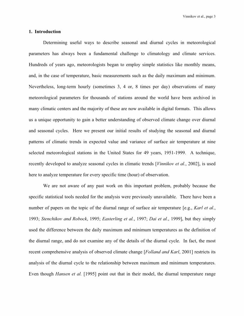
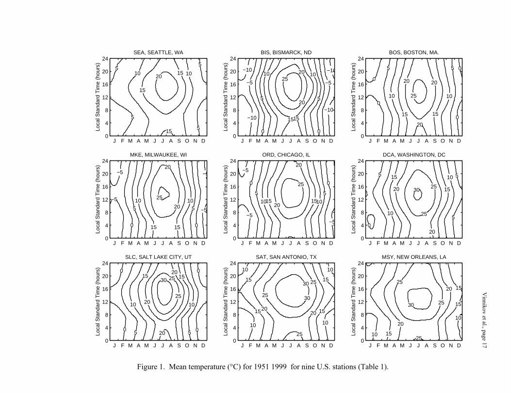
The results of the calculations for each of the nine stations are presented in Figures 1-4.

Figure 1 displays the average of the seasonal and diurnal patterns of expected values average for

1951, the first year of record, and 1999, the last year of record. Both these years occupy the

same position in the leap year cycle. If we ignore this four-year cycle, we can consider the

estimates presented in Figure 1 as an approximation of the multi-year 1951-1999 average of

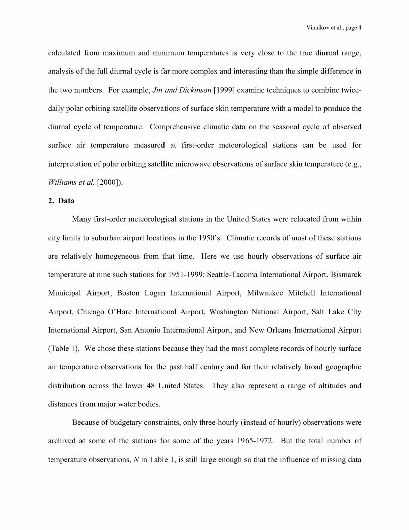
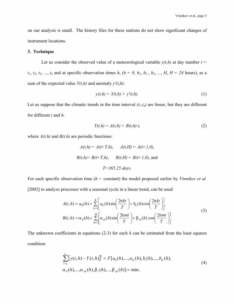
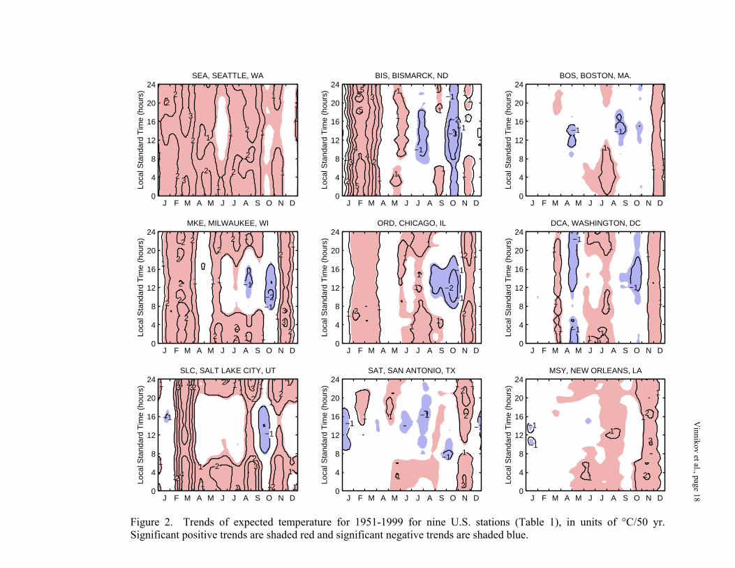
expected values. Figure 2 gives the pattern of linear trends of expected values. Standard

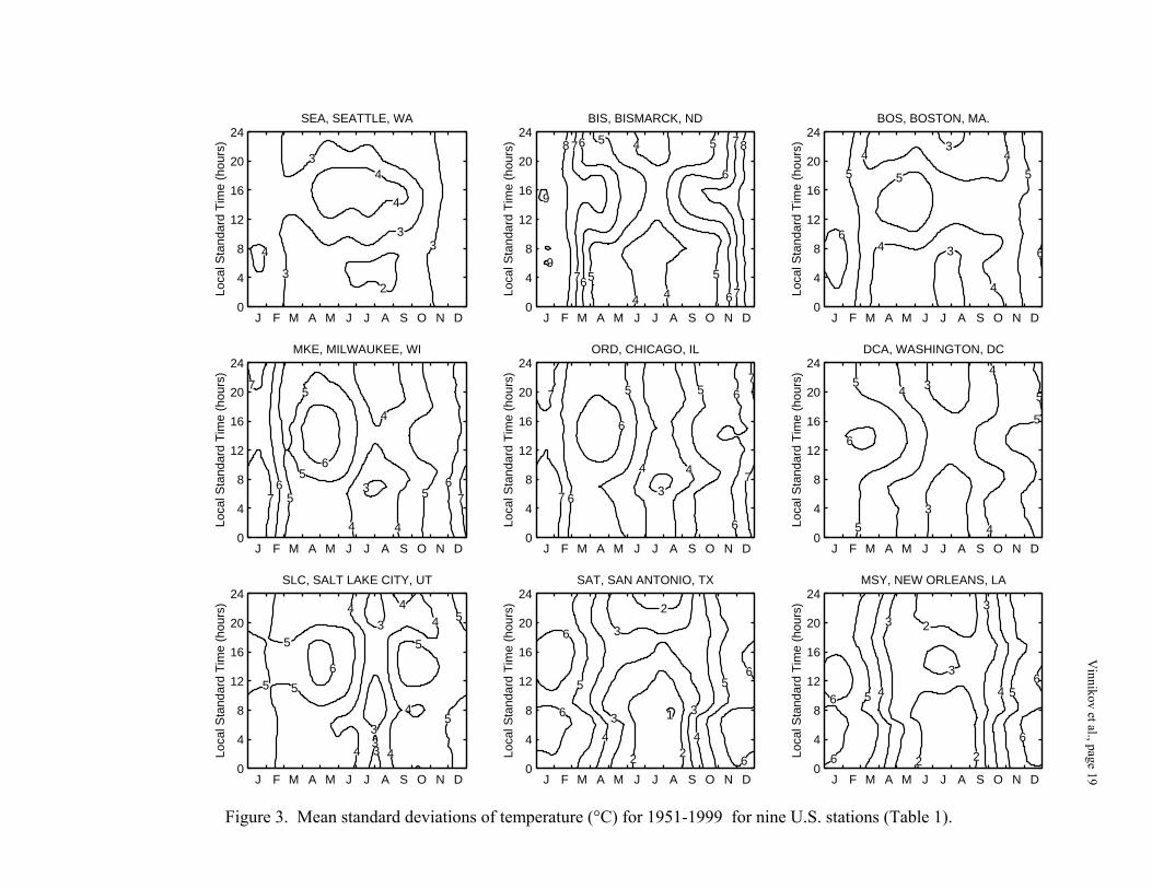
deviations shown in Figure 3 are calculated from the average of variances estimated for years

1951 and 1999. They approximately represent the multi-year average of variances for the 1951-

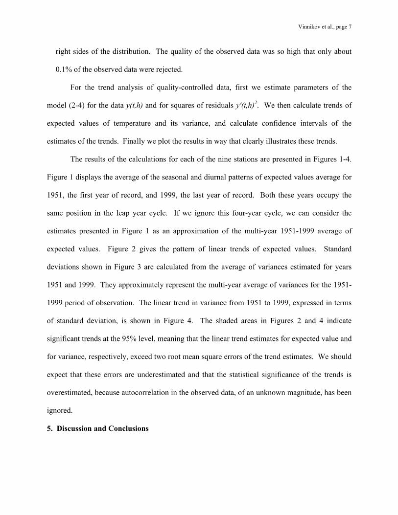
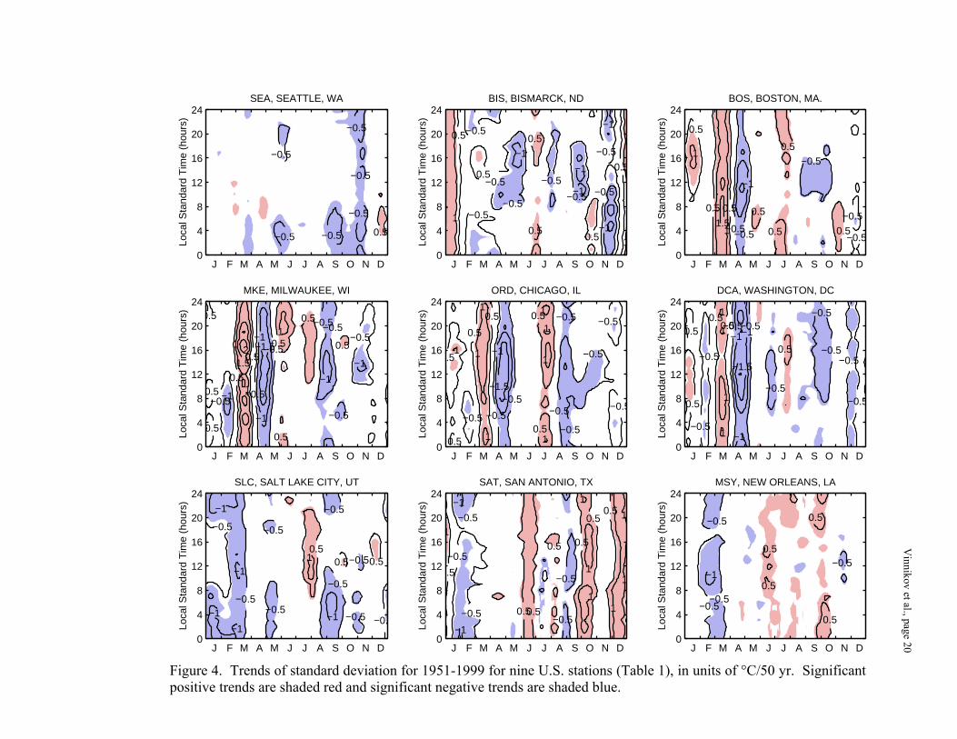
1999 period of observation. The linear trend in variance from 1951 to 1999, expressed in terms

of standard deviation, is shown in Figure 4. The shaded areas in Figures 2 and 4 indicate

significant trends at the 95% level, meaning that the linear trend estimates for expected value and

for variance, respectively, exceed two root mean square errors of the trend estimates. We should

expect that these errors are underestimated and that the statistical significance of the trends is

overestimated, because autocorrelation in the observed data, of an unknown magnitude, has been

ignored.

5. Discussion and Conclusions


Figures 1-4 reveal many significant changes in the seasonal and diurnal variation of

temperature during the past half-century. Significant warming dominates the pattern for all

stations, but the patterns are very complex. Diurnal asymmetry of the warming is evident for

some stations, but only in the summer and fall, in agreement with an analysis using seasonal

averages of daily maximum and minimum temperatures [Karl et al., 1993]. However our new

technique shows these patterns in much more detail. There is no correspondence between the

trends in temperature and the trends in temperature variability.

The standard deviation was largest in the winter at all times of day, but in the summer

only in the daytime. There was no general trend in standard deviation, with as many positive

trends as negative, and no evidence of diurnal asymmetry of the trends. However, Boston,

Milwaukee, Chicago, and Washington all had upward trends in March and downward trends in

April. Three of the stations, with the exception of Boston, have a significant warming at all

times of the day in March. One interpretation of these patterns is to associate the trends of

variance and mean temperature with an earlier arrival of spring, with its variable transitional

weather and more fluctuation of warm and cold advection. In contrast, this transitional, variable

weather is reduced in April, but there is a small cooling trend in April, but it is only significant in

Washington and at some times in Boston. Our technique could also be applied to wind or other

measure of storminess, such as precipitation, to investigate these patterns further. Here we

present them only as an illustration of their potential for studying climate change in detail. For

each region of the country, we now point out more specific findings:

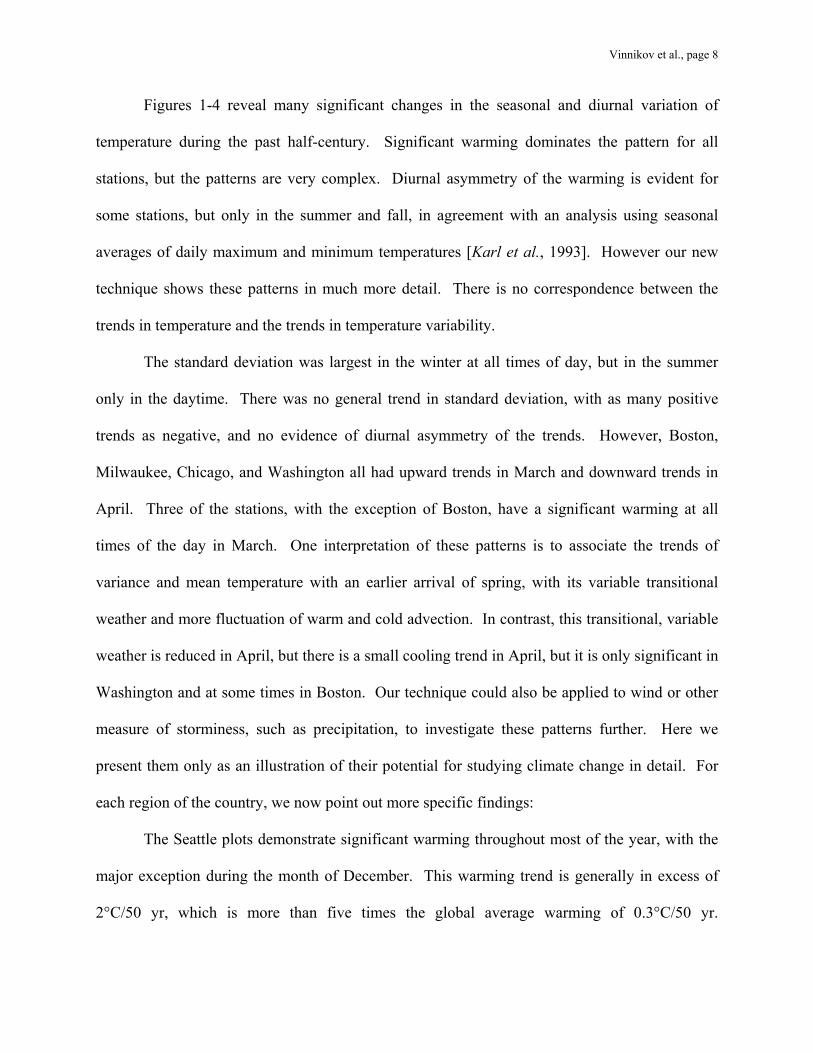
The Seattle plots demonstrate significant warming throughout most of the year, with the

major exception during the month of December. This warming trend is generally in excess of

2°C/50 yr, which is more than five times the global average warming of 0.3°C/50 yr.


Temperature increases are consistently higher in the nighttime and morning hours, which agrees

with findings of other authors (e.g., Karl et al. [1993]). Moreover, the warming is generally

greatest during the nighttime in late winter and early spring. In contrast, the warming trend is

smallest during the daylight hours in the warm half of the year (excepting the month of

December). There are no major changes in standard deviation, except that it decreased during

the month of November.

It is very interesting that a maritime location would experience such significant warmth.

We wonder whether changes in sea breezes during the evening and early morning hours could

have a direct impact on these warming trends. A similar plot of wind speed and direction could

illuminate the link between temperature trends and wind patterns. Therefore, we encourage the

expansion the technique used in this article to parameters other than temperature.

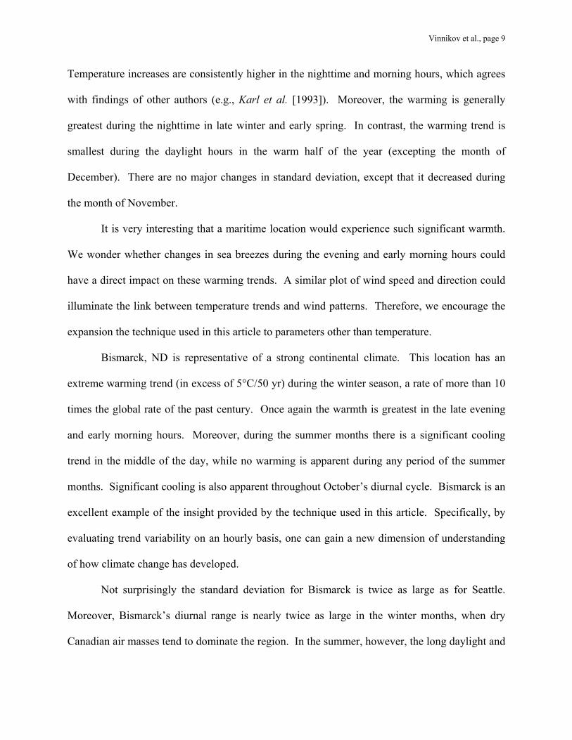
Bismarck, ND is representative of a strong continental climate. This location has an

extreme warming trend (in excess of 5°C/50 yr) during the winter season, a rate of more than 10

times the global rate of the past century. Once again the warmth is greatest in the late evening

and early morning hours. Moreover, during the summer months there is a significant cooling

trend in the middle of the day, while no warming is apparent during any period of the summer

months. Significant cooling is also apparent throughout October’s diurnal cycle. Bismarck is an

excellent example of the insight provided by the technique used in this article. Specifically, by

evaluating trend variability on an hourly basis, one can gain a new dimension of understanding

of how climate change has developed.

Not surprisingly the standard deviation for Bismarck is twice as large as for Seattle.

Moreover, Bismarck’s diurnal range is nearly twice as large in the winter months, when dry

Canadian air masses tend to dominate the region. In the summer, however, the long daylight and


increased humidity diminished the diurnal temperature range. In terms of changes in standard

deviation, there is a short period of increased variability in January, and decreased variability in

spring and autumn daylight hours.

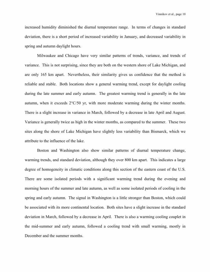
Milwaukee and Chicago have very similar patterns of trends, variance, and trends of

variance. This is not surprising, since they are both on the western shore of Lake Michigan, and

are only 165 km apart. Nevertheless, their similarity gives us confidence that the method is

reliable and stable. Both locations show a general warming trend, except for daylight cooling

during the late summer and early autumn. The greatest warming trend is generally in the late

autumn, when it exceeds 2°C/50 yr, with more moderate warming during the winter months.

There is a slight increase in variance in March, followed by a decrease in late April and August.

Variance is generally twice as high in the winter months, as compared to the summer. These two

sites along the shore of Lake Michigan have slightly less variability than Bismarck, which we

attribute to the influence of the lake.

Boston and Washington also show similar patterns of diurnal temperature change,

warming trends, and standard deviation, although they over 800 km apart. This indicates a large

degree of homogeneity in climatic conditions along this section of the eastern coast of the U.S.

There are some isolated periods with a significant warming trend during the evening and

morning hours of the summer and late autumn, as well as some isolated periods of cooling in the

spring and early autumn. The signal in Washington is a little stronger than Boston, which could

be associated with its more continental location. Both sites have a slight increase in the standard

deviation in March, followed by a decrease in April. There is also a warming cooling couplet in

the mid-summer and early autumn, followed a cooling trend with small warming, mostly in

December and the summer months.


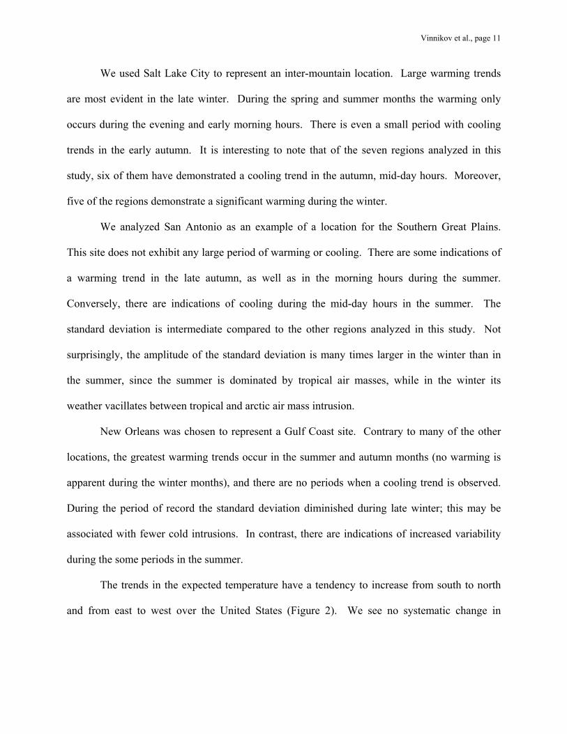
We used Salt Lake City to represent an inter-mountain location. Large warming trends

are most evident in the late winter. During the spring and summer months the warming only

occurs during the evening and early morning hours. There is even a small period with cooling

trends in the early autumn. It is interesting to note that of the seven regions analyzed in this

study, six of them have demonstrated a cooling trend in the autumn, mid-day hours. Moreover,

five of the regions demonstrate a significant warming during the winter.

We analyzed San Antonio as an example of a location for the Southern Great Plains.

This site does not exhibit any large period of warming or cooling. There are some indications of

a warming trend in the late autumn, as well as in the morning hours during the summer.

Conversely, there are indications of cooling during the mid-day hours in the summer. The

standard deviation is intermediate compared to the other regions analyzed in this study. Not

surprisingly, the amplitude of the standard deviation is many times larger in the winter than in

the summer, since the summer is dominated by tropical air masses, while in the winter its

weather vacillates between tropical and arctic air mass intrusion.

New Orleans was chosen to represent a Gulf Coast site. Contrary to many of the other

locations, the greatest warming trends occur in the summer and autumn months (no warming is

apparent during the winter months), and there are no periods when a cooling trend is observed.

During the period of record the standard deviation diminished during late winter; this may be

associated with fewer cold intrusions. In contrast, there are indications of increased variability

during the some periods in the summer.

The trends in the expected temperature have a tendency to increase from south to north

and from east to west over the United States (Figure 2). We see no systematic change in


temperature variability (Figure 4), except for the late winter/early spring dipole in the northeast

United States discussed earlier.

Figures 1-4 give a comprehensive picture of the observed changes in hourly temperature

and its variability during the last 50 years at many U.S. stations. They also show which parts of

these changes were statistically significant. The observed changes are very complicated. They

cannot be interpreted as simply as the results of earlier research of trends in monthly averages of

maximum and minimum temperature. The results we present do not contradict conclusions of

the earlier research, yet they demonstrate how our technique can provide valuable new insight

and more detailed interpretation of the climatic changes.

Representativeness of the first-order stations at major airports is always questionable.

For example, Foster and Leffler [1981] found that the Washington National Airport station

(DCA) is inside of Washington, DC’s heat island. But as compared to the temperature records of

other meteorological stations in the region (the first-order station BWI, Baltimore, MD airport;

an urban station, Baltimore Customs House; and a rural station, Woodstock, MD) we found that

its heat island is stable and the station can be used in trend analyses.

Our technique allows the estimation of the expected values of the main moments of the

statistical distribution of meteorological variables for every hour h of every day t from the period

of observations. The technique is not sensitive to gaps in the data. Polynomial or other

functions can be used instead of linear trends. The technique can be extended for the case when

times of observations are different for different parts of the record. This analysis may be used as

a prototype for developing the next generation of climate services, which will be able to supply

customers with detailed information about moments of the statistical distribution of many

meteorological variables for each day and each hour of the period of observation.


Acknowledgments. We thank Abram Kagan, Benjamin Kedem, Anandu Vernekar, Eugene

Rasmusson, Semyon Grodsky, and Robert J. Leffler for valuable discussions, and reviewer Dale

Kaiser for extremely useful suggestions for improving the text of the paper. We thank

NCDC/NOAA and especially Thomas C. Peterson, Neal J. Lott, Milton S. McCown, Sharon

Capps-Hill, Harry W. Hahlberg, and Devoyd Ezell for support, data, and consultations. The

work is sponsored by NOAA grants NAO6GPO403 and NA17EC1483, NASA grant

NAG510746, and the New Jersey Agricultural Experiment Station.


References

Dai, A., K. E. Trenberth, and T. R. Karl, Effects of clouds, soil moisture, precipitation and water

vapor on diurnal temperature range, J. Climate, 12, 2451-2473, 1999.

Easterling, D. R., B. Horton, P. D. Jones, T. C. Peterson, T. R. Karl, D. E. Parker, M. J. Salinger,

V. Razuvaev, N. Plummer, P. Jamason, and C. K. Folland, Maximum and minimum

temperature trends for the globe, Science, 277, 345-347, 1997.

Folland, C. K., and T. R. Karl, Observed Climate Variability and Change, Chapter 2 of Climate

Change 2001: The Scientific Basis, edited by Houghton et al., Cambridge Univ. Press,

Cambridge, UK, 99-181, 2001.

Foster, J. L., and R. J. Leffler, Unrepresentative temperatures at a first-order meteorological

station: Washington National Airport, Bull. Am. Meteor. Soc., 62, 1002-1006, 1981.

Hansen, J., M. Sato, and R. Ruedy, Long-term changes of the diurnal temperature cycle:

Implications about mechanisms of global climate change, Atmos. Res., 37, 175-209, 1995.

Jin, M., and R. E. Dickinson, Interpolation of surface radiation temperature measured from polar

orbiting satellites to a diurnal cycle. Part 1: Without clouds, J. Geophys. Res., 104, 2105-2116,

1999.

Karl, T. R., P. D. Jones, R. W. Knight, G. Kukla, N. Plummer, V. Razuvayev, K. P. Gallo, J.

Lindseay, R. J. Charlson, and T. C. Peterson, Asymmetric trends of daily maximum and

minimum temperature, Bull. Am. Meteor. Soc., 74, 1007-1023, 1993.

Stenchikov, G. L., and A. Robock, Diurnal asymmetry of climatic response to increased CO2 and

aerosols: Forcings and feedbacks. J. Geophys. Res., 100, 26,211-26,227, 1995.

Vinnikov, K. Y., and A. Robock, Trends in moments of climatic indices. Geophys. Res. Lett., 29

(2), 10.1029/2001GL014025, 2002.


Vinnikov, K. Y., A. Robock, D. J. Cavalieri, and C. L. Parkinson, Analysis of seasonal cycles in

climatic trends with application to satellite observations of sea ice extent, Geophys. Res. Lett.,

2002, in press.

Williams, C. N., A. Basist, T. C. Peterson, and N, Grody, Calibration and verification of land

surface temperature anomalies derived from the SSM/I, Bull. Am. Meteor. Soc., 81, 2141-

2156, 2000.


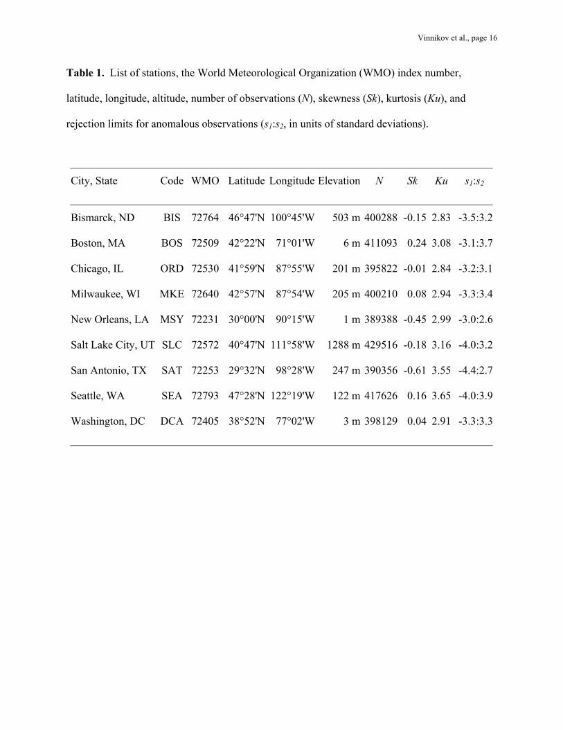
Table 1. List of stations, the World Meteorological Organization (WMO) index number,

latitude, longitude, altitude, number of observations (N), skewness (Sk), kurtosis (Ku), and

rejection limits for anomalous observations (s1:s2, in units of standard deviations).

City, State Code WMO Latitude Longitude Elevation N Sk Ku s1:s2

Bismarck, ND BIS 72764 46°47'N 100°45'W 503 m 400288 -0.15 2.83 -3.5:3.2

Boston, MA BOS 72509 42°22'N 71°01'W 6 m 411093 0.24 3.08 -3.1:3.7

Chicago, IL ORD 72530 41°59'N 87°55'W 201 m 395822 -0.01 2.84 -3.2:3.1

Milwaukee, WI MKE 72640 42°57'N 87°54'W 205 m 400210 0.08 2.94 -3.3:3.4

New Orleans, LA MSY 72231 30°00'N 90°15'W 1 m 389388 -0.45 2.99 -3.0:2.6

Salt Lake City, UT SLC 72572 40°47'N 111°58'W 1288 m 429516 -0.18 3.16 -4.0:3.2

San Antonio, TX SAT 72253 29°32'N 98°28'W 247 m 390356 -0.61 3.55 -4.4:2.7

Seattle, WA SEA 72793 47°28'N 122°19'W 122 m 417626 0.16 3.65 -4.0:3.9

Washington, DC DCA 72405 38°52'N 77°02'W 3 m 398129 0.04 2.91 -3.3:3.3


Loca

l Sta

ndar

d T

ime

(hou

rs)

SEA, SEATTLE, WA

5

5

5

5

10 10

15

15

15

20

J F M A M J J A S O N D0

4

8

12

16

20

24

Loca

l Sta

ndar

d T

ime

(hou

rs)

BIS, BISMARCK, ND

−10

−10

−10

−10

−5 −5

0 0

5 5

10 10

1515

20

2025


4

8

12

16

20

24

Loca

l Sta

ndar

d T

ime

(hou

rs)

BOS, BOSTON, MA.

0

0

0

0

5 5

10 10

15 15

20 20

20

25


4

8

12

16

20

24

Loca

l Sta

ndar

d T

ime

(hou

rs)

MKE, MILWAUKEE, WI

−5

−5

−5

−5

0 0

5 510 10

15 15

20

20

25


4

8

12

16

20

24

Loca

l Sta

ndar

d T

ime

(hou

rs)

ORD, CHICAGO, IL

−5

−5−5

0 0

5 5

10 1015 1520

20

25


4

8

12

16

20

24

Loca

l Sta

ndar

d T

ime

(hou

rs)

DCA, WASHINGTON, DC

0

5 5

5

5

10

1015

1520

20

25

2530


4

8

12

16

20

24

Loca

l Sta

ndar

d T

ime

(hou

rs)

SLC, SALT LAKE CITY, UT

0

0

0

05 5

10 10

15 15

20

20

20

25

2530


4

8

12

16

20

24

Loca

l Sta

ndar

d T

ime

(hou

rs)

SAT, SAN ANTONIO, TX

10

10

10

10

15

15

15

152020

25

25

25

30

30


4

8

12

16

20

24

Loca

l Sta

ndar

d T

ime

(hou

rs)

MSY, NEW ORLEANS, LA

10

10

15

15

15

20

2025

25

25

30


4

8

12

16

20

24

Figure 1. Mean temperature (°C) for 1951 1999 for nine U.S. stations (Table 1).


Loca

l Sta

ndar

d T

ime

(hou

rs)

SEA, SEATTLE, WA

1

1

1

1 1

1

1

12

2

2

2

2

2

2

2

3

3


4

8

12

16

20

24

Loca

l Sta

ndar

d T

ime

(hou

rs)

BIS, BISMARCK, ND

−3

−2

−1

−1

−11

1

1

1

1

1

1

11

1

1

1

2

23

3

44

5

5

5

5


4

8

12

16

20

24

Loca

l Sta

ndar

d T

ime

(hou

rs)

BOS, BOSTON, MA.

−1−1

1 1

1


4

8

12

16

20

24

Loca

l Sta

ndar

d T

ime

(hou

rs)

MKE, MILWAUKEE, WI

−2−1

−1

1

1 1 1

1

1

11

1

2

2

2

22

2

2

2

2

2

2

2

2

23

3


4

8

12

16

20

24

Loca

l Sta

ndar

d T

ime

(hou

rs)

ORD, CHICAGO, IL

−2

−1

−1

11

1

1

1 1

1

1

1

1

2

22


4

8

12

16

20

24

Loca

l Sta

ndar

d T

ime

(hou

rs)

DCA, WASHINGTON, DC

−1

−1

−1

1

1

1 1

1

1

1

11

1


4

8

12

16

20

24

Loca

l Sta

ndar

d T

ime

(hou

rs)


−1

−1

1

11

1

1

1

1

1

1

1

1

1

1

1

2

22

2

2

2

2

2

3 3 3

3

4 4

4


4

8

12

16

20

24

Loca

l Sta

ndar

d T

ime

(hou

rs)


−1 −1

−1

−1

1 1

1

1 1

1

2

2

2


4

8

12

16

20

24

Loca

l Sta

ndar

d T

ime

(hou

rs)


−1

−1

1

1

1

1

2

2

2


4

8

12

16

20

24

Figure 2. Trends of expected temperature for 1951-1999 for nine U.S. stations (Table 1), in units of °C/50 yr.Significant positive trends are shaded red and significant negative trends are shaded blue.


Loca

l Sta

ndar

d T

ime

(hou

rs)

SEA, SEATTLE, WA

2

3

3

3

34

4

4


4

8

12

16

20

24

Loca

l Sta

ndar

d T

ime

(hou

rs)

BIS, BISMARCK, ND

4

4 4

5

5

5

5

6

6

6

6

7

7

7

7

8 8

9

9


4

8

12

16

20

24

Loca

l Sta

ndar

d T

ime

(hou

rs)

BOS, BOSTON, MA.

3

3

4 4

4

4

5 55

6

6


4

8

12

16

20

24

Loca

l Sta

ndar

d T

ime

(hou

rs)

MKE, MILWAUKEE, WI

3

4

4 4

5 5

5

56 6

6

7

7 7


4

8

12

16

20

24

Loca

l Sta

ndar

d T

ime

(hou

rs)

ORD, CHICAGO, IL

3

4 4

5 5

6

6

6

6

7

7

7

7


4

8

12

16

20

24

Loca

l Sta

ndar

d T

ime

(hou

rs)

DCA, WASHINGTON, DC

3

3

4

4

4

5

5

5

5

6


4

8

12

16

20

24

Loca

l Sta

ndar

d T

ime

(hou

rs)


3

3

33

4

4

4

4

4

4

5

5

5

5

5

5

6


4

8

12

16

20

24

Loca

l Sta

ndar

d T

ime

(hou

rs)


1

2

2 2

3

33

4 4

5 5

6

6

6

6


4

8

12

16

20

24

Loca

l Sta

ndar

d T

ime

(hou

rs)


2

2 2

33

3

4 45 56

6

6

6


4

8

12

16

20

24

Figure 3. Mean standard deviations of temperature (°C) for 1951-1999 for nine U.S. stations (Table 1).


Loca

l Sta

ndar

d T

ime

(hou

rs)

SEA, SEATTLE, WA

−0.5

−0.5

−0.5

−0.5−0.5

−0.5

0.5


4

8

12

16

20

24

Loca

l Sta

ndar

d T

ime

(hou

rs)

BIS, BISMARCK, ND

−1

−1

−1

−1

−1

−0.5

−0.5

−0.5

−0.5−0.5−0.5

−0.5 −0.5

0.5

0.50.5

0.5

0.5

0.51

1

1

1


4

8

12

16

20

24

Loca

l Sta

ndar

d T

ime

(hou

rs)

BOS, BOSTON, MA.

−1

−0.5−0.5 −0.5

−0.5

−0.5

0.5 0.5

0.5

0.5

0.5

0.5

0.51

1

1

1.5


4

8

12

16

20

24

Loca

l Sta

ndar

d T

ime

(hou

rs)

MKE, MILWAUKEE, WI

−1.5

−1

−1

−1

−1

−1

−0.5−0.5

−0.5

−0.5−0.5−0.5

−0.5

0.5

0.5

0.5

0.50.5

0.5

0.5

0.5

0.5

1

1

1

1.52


4

8

12

16

20

24

Loca

l Sta

ndar

d T

ime

(hou

rs)

ORD, CHICAGO, IL

−1.5

−1

−0.5

−0.5−0.5

−0.5

−0.5

−0.5

−0.5−0.5

−0.5

0.5

0.5 0.5

0.5

0.5

0.5

1

1

1

1

1

1

1

1


4

8

12

16

20

24

Loca

l Sta

ndar

d T

ime

(hou

rs)

DCA, WASHINGTON, DC

−1.5

−1−1

−1−0.5

−0.5

−0.5−0.5

−0.5

−0.5

−0.5

−0.5

−0.5

0.50.5

0.5

0.5

0.5

1

1

1

1


4

8

12

16

20

24

Loca

l Sta

ndar

d T

ime

(hou

rs)


−1

−1

−1

−1

−1

−0.5−0.5

−0.5

−0.5

−0.5

−0.5

−0.5

−0.5

−0.5

0.50.50.51


4

8

12

16

20

24

Loca

l Sta

ndar

d T

ime

(hou

rs)


−1

−1

−0.5

−0.5

−0.5−0.5

−0.50.5

0.50.5

0.5

0.50.5

0.5

1

1

1

1

1

1

1


4

8

12

16

20

24

Loca

l Sta

ndar

d T

ime

(hou

rs)


−1

−0.5

−0.5−0.5

−0.5

0.5

0.5

0.5

0.5


4

8

12

16

20

24

Figure 4. Trends of standard deviation for 1951-1999 for nine U.S. stations (Table 1), in units of °C/50 yr. Significantpositive trends are shaded red and significant negative trends are shaded blue.

Documents

Diurnal and Seasonal Cycles of Trends of Surface Air ...climate.envsci.rutgers.edu/pdf/hourly16jgrRevision.pdf · Diurnal and Seasonal Cycles of Trends of ... seasonal cycles of trends