DISCUSSION PAPER SERIES

IZA DP No. 10968

Achmad TohariChristopher ParsonsAnu Rammohan

Targeting Poverty under Complementarities:Evidence from Indonesia’s Unified Targeting System

AUGUST 2017

Any opinions expressed in this paper are those of the author(s) and not those of IZA. Research published in this series may include views on policy, but IZA takes no institutional policy positions. The IZA research network is committed to the IZA Guiding Principles of Research Integrity.The IZA Institute of Labor Economics is an independent economic research institute that conducts research in labor economics and offers evidence-based policy advice on labor market issues. Supported by the Deutsche Post Foundation, IZA runs the world’s largest network of economists, whose research aims to provide answers to the global labor market challenges of our time. Our key objective is to build bridges between academic research, policymakers and society.IZA Discussion Papers often represent preliminary work and are circulated to encourage discussion. Citation of such a paper should account for its provisional character. A revised version may be available directly from the author.

Schaumburg-Lippe-Straße 5–953113 Bonn, Germany

Phone: +49-228-3894-0Email: publications@iza.org www.iza.org

IZA – Institute of Labor Economics

DISCUSSION PAPER SERIES

IZA DP No. 10968

Targeting Poverty under Complementarities:Evidence from Indonesia’s Unified Targeting System

AUGUST 2017

Achmad TohariUniversity of Western Australia and Airlangga University

Christopher ParsonsUniversity of Western Australia, University of Oxford and IZA

Anu RammohanUniversity of Western Australia

ABSTRACT

IZA DP No. 10968 AUGUST 2017

Targeting Poverty under Complementarities:Evidence from Indonesia’s Unified Targeting System*

Combining nationally representative administrative and survey data with official proxy means

testing models and coefficients, we evaluate Indonesia’s three largest social programs.

The setting for our evaluation is the launch of Indonesia’s Unified Targeting system, an

innovation developed to reduce targeting errors and increase program complementarities.

Introducing a new method of evaluation under the condition of multiple programs, we

show that households receiving all three programs are at least 30 percentage points better

off than those receiving none. Importantly, the bias from failing to account for program

complementarities is greater in magnitude than the benefits of receiving a single program.

JEL Classification: D04, I32, I38, O12

Keywords: poverty, targeting, Indonesia, complementarities

Corresponding author:Christopher ParsonsEconomics (UWA Business School)University of Western Australia35 Stirling HighwayCrawley WA 6009Australia

E-mail: christopher.parsons@uwa.edu.au

* We gratefully acknowledge generous funding from the Australian government through Department of Foreign

Af-fairs and Trade (DFAT) and data support from the TNP2K. We are also grateful to Bambang Widianto, Sudarno

Sumarto, Elan Satriawan, Aufa Doarest, Priadi Asmanto, Gracia Hadiwidjaja (TNP2K), Vivi Alatas, Hendratmo Tuhiman,

Taufik Hidayat (World Bank), Ken Clements (UWA) and Benjamin Olken (MIT) as well as seminar participants both in

TNP2K and the University of Western Australia for their valuable comments.

2

Introduction

“I can live for two months on a good compliment”

Mark Twain

Targeted poverty programs represent important interventions to reduce poverty in developing

countries. Delivering and evaluating these programs are challenging however, specifically

with regards to accurately differentiating between poor and non-poor households. Indonesia

has a long history of targeted social programs, and since 2005, the Indonesian government

has experimented with several methods to identify and access vulnerable groups. These

include geographical targeting, community-based targeting and proxy-means testing (World

Bank 2012a). Studies by Alatas, et al. (2012) and Cameron and Shah (2014) however, show

that a significant proportion of poor households do not benefit from targeted poverty

programs in Indonesia.

To address these concerns, the Government of Indonesia (GoI) developed a Unified

Targeting System (UDB), called the Basis Data Terpadu or Unified Database, through the

establishment of TNP2K1 under the auspices of the Office of the Vice-President of

Indonesia and the Indonesian Central Bureau of Statistics (BPS). The unified targeting

system approach is typically used to deliver social assistance programs in OECD countries

(Grosh et al. 2008), but is rarely implemented in developing countries due to a lack of

(complete) information on household welfare.2 The primary objectives of the UDB are to

reduce targeting errors and to increase the complementarities between various poverty

programs, by ensuring that poor households receive complementary benefits from multiple

programs (TNP2K 2015). The GoI allocates a significant portion of its fiscal expenditure

(about 11.5% of total expenditure in 2016), towards social programs. The three flagship

social programs are: Health Insurance for the Poor (Asuransi Kesehatan untuk Keluarga

Miskin, or Askeskin, later renamed Jamkesmas), Rice for the Poor (Beras Miskin, or Raskin)

and Unconditional Cash Transfers (Bantuan Langsung Tunai, or BLT, later renamed

BLSM).3

1 Tim Nasional Percepatan Penanggulangan Kemiskinan or the National Team for Accelerating Poverty

Reduction. 2 Examples of the use of the unified database for targeting social protection programs in developing countries

include the Cadastro Unico program in Brazil (De la Brière and Lindert 2005) and the SISBEN System in

Columbia (Castaneda and Fernandez 2005). 3 We are unable to evaluate Indonesia’s smaller social programs such as scholarship for the poor (Bantuan Siswa

Miskin, or BSM), the Conditional Cash Transfer program (Program Keluarga Harapan, or PKH) and

3

Although previous studies have evaluated Indonesia’s targeting system they have some

drawbacks. For example, studies using field experiments (Alatas et al. 2012; Alatas, et al.

2016) are restricted to small samples across a few villages. This limits their ability to

produce externally valid results. Second, previous research has only been able to evaluate

single programs. For example, Sparrow (2008) and Sparrow et al. (2013) study the Askeskin

and Jamkesmas programs; Sumarto et al. (2003) and Olken (2005) study the Raskin

program; and Alatas et al. (2016) evaluate the Conditional Cash Transfer Program.

Evaluating programs in isolation may lead to upward biases since individuals’ outcomes

might otherwise be driven by omitted programs. We address both these concerns.

More specifically, in this paper, we evaluate the impact of the introduction of Indonesia’s

Unified Targeting System on the targeting and delivery of Indonesia’s three largest social

programs. We contribute to the literature on poverty targeting through introducing a new

method of evaluating poverty targeting under the condition of multiple concurrent programs

that a priori are expected to complement one another. We subsequently test our method

using nationally representative data in conjunction with the official Proxy Means Test

(PMT) coefficients and models, thereby exploiting the design of the poverty program. This

approach has been argued to be first best when analysing social programs that target poverty

(Ravallion 2007). Understanding these complementarities is important since interventions

nearly always occur alongside with one another (Grosh et al. 2008); and multifaceted

programs for ‘ultra-poor’ households may have a significantly positive and persistent impact

on their chances of exiting poverty (Banerjee, et al. 2015b).

We show that the introduction of the UDB significantly increased the successful targeting of

social programs in Indonesia. The probability of targeted households receiving all three

programs increased by 117% compared to previous targeting efforts. Households receiving

all three programs, experienced an increase in household expenditure of 30 percentage

points compared to those that received no programs, and increases of between 16 and 19

percentage points compared to households that received only one or two programs. In other

words, our results show that conventional poverty targeting performance evaluations are

biased upwards, since they omit the impacts of complimentary programs. Taken together our

results justify the implementation of the UDB to improve program targeting and program

complementarities between social programs.

community block grants for education and development (Widianto 2013), since their coverage is not nationwide

and in the case of the BSM, beneficaries are nominiated by their teachers.

4

The rest of the paper is organised as follows. We discuss the evolution of Indonesia’s social

protection programs and the introduction of the Unified Targeting System in Section 2. In

Section 3, we outline our approach to evaluate Targeting Under Complementarities. We then

describe the datasets used in the analysis. In Section 4, we evaluate the introduction of the

Unified Targeting System on the targeting performance of Indonesia’s three most important

social programs. Section 5 presents an evaluation of the impact of different program

combinations on household per capita expenditure and poverty, thereby highlighting the

important role of program complementarities. Finally, the conclusions are presented in

Section 6.

Background

History of Indonesian Poverty Programs

The definition of the poverty line in Indonesia has evolved several times, since its

introduction in 1975 (see Priebe 2014). Nevertheless, the majority of the Indonesian

population hovers around the national poverty threshold (World Bank 2012a) with

approximately half the population living below IDR15,000 per day (around PPP USD 2.25 a

day). Marginal shocks therefore have profound effects on household welfare in Indonesia

(Pritchett et al. 2000, and Suryahadi et al. 2003). This has made poverty and vulnerability

central policy issues for successive Governments.

The GoI introduced social security programs for the first time in 1997 to mitigate the adverse

economic and social impact of the Asian Financial Crisis (Daly and Fane 2002; Bacon and

Kojima 2006; Grosh et al. 2008; Sumarto and Bazzi 2011).4 These, the first generation of

Indonesia’s social protection programs, called Jaring Pengaman Sosial (JPS), were

implemented under President Habibie’s Administration in 1999/2000 (Widjaja 2012). The

JPS sought to protect chronically poor households from falling further into poverty while

eliminating vulnerable households’ exposure to risk (Sumarto et al. 2002). The JPS was

tasked with: (i) ensuring the availability of affordable food through the OPK (for Operasi

Pasar Khusus or Special Market Operation program); (ii) improving household purchasing

power through employment creation; (iii) preserving access to critical social services,

particularly health through the Askeskin (for Asuransi Kesehatan Penduduk Miskin or health

4 Please refer to Figure A1 in the Appendix, which summarizes the evolution of social safety net in Indonesia

from 1997 to 2008.

5

insurance for the poor program), education through the BOS (for Bantuan Operasional

Sekolah or school block grant program); and (iv) sustaining the local economy through

regional block grants and the extension of small-scale credit.5 In 2002, the GoI changed the

OPK to become one of the largest social protection programs named Raskin (Beras untuk

Keluarga Miskin or Rice for the Poor), which aimed to reduce household spending on food,

especially on rice.

The second generation of social protection programs were implemented between 2005 and

2008 to alleviate the financial burden on households from rising oil prices (Bacon and

Kojima 2006). To mitigate the negative effects, especially on poor and near-poor households,

the GoI launched the Fuel Subsidy Reduction Compensation Program, namely Program

Kompensasi Pengurangan Subsidi Bahan Bakar Minyak (PKPS-BBM) (World Bank 2006,

Yusuf and Resosudarmo 2008 and Rosfadhila et al. 2011). Under this scheme, an

Unconditional Cash Transfer program was introduced to complement the BLT (for Bantuan

Likuiditas Tunai or Direct Cash Assistance). This program was subsequently renamed BLSM

(for Bantuan Langsung Sementara Masyarakat or Temporary Unconditional Cash Transfer

program) in 2013.6 From July to September 2005, the GoI through Statistics Indonesia

(Badan Pusat Statistik or BPS) conducted a census of poor households for the first time, with

the aim of implementing the BLT program. The database was also known as PSE05

(Pendataan Sosial Ekonomi Penduduk 2005, or Socio-economic Data Collection of the

Population).7

In 2008, the GoI once again restructured the nationwide programs. At this time the

government’s three main flagship program were the BLT, Raskin and Jamkesmas (see figure

1). These three programs target the same beneficiaries, the poor and the near-poor

households, or those households that are 20% above the poverty line, covering 22% of total

households in 2009. From the perspective of budget disbursement, BLT spending constitutes

40% of total social assistance expenditure, Raskin accounts for 34% and Jamkesmas for 13%

(Jellema and Noura 2012).

5 The GoI disbursed IDR3.9 trillion directly to JPS programs out of a total development budget of IDR14.2

trillion, with financial support from international donors including the World Bank and the Asian Development

Bank (Sumarto and Bazzi, 2011). 6 Under this program, the targeted household received cash transfers delivered via post office (Bazzi et al.

2015). The BLT cash benefit was IDR100,000 (roughly US$10) per month to each targeted recipient household

and it was increased to IDR150,000 under the BLSM scheme. 7 The data collection involved community-based nominations combined with other data to identify prospective

beneficiary households based on fourteen selected indicators that represented the well-being of poor households,

see Hastuti et al. (2006) for further details.

6

Introduction of the UDB

Due to concerns about the poor performance of the PSE05,8 in 2008-2009 the GoI updated

the list of beneficiaries by including community verification. This updated version, was

known as the PPLS08 (Pendataan Program Lindungan Sosial 2008, or Data Collection for

Targeting Social Protection Programs). As with PSE05, this database was primarily used to

identify eligible households for unconditional cash transfers. Due to time constraints

however, the problems associated with PPLS08 were similar or worse than those of the

PSE05 and errors in targeting continued (Rosfadhila et al. 2011). Some argue that targeting

errors catalysed social unrest (Widjaja 2009; Cameron and Shah 2014).

Explanations for the poor performance of targeting mechanisms and the absence of

complementarities in the social protection programs over the period 2005 and 2008 include:

(1) alternative methods of targeting implemented by each of the poverty programs;9 (2)

biased results from the targeting design;10 and (3) different notions of poverty between the

views of the community or local leader and the central government. This may have led to

some of the programs being diverted away from intended beneficiaries (Olken 2005; Alatas

et al., 2012). In 2010 the TNP2K was mandated with the task of reducing the prevalence of

poverty to 8% by 2014 and was given the responsibility of overseeing the coordination of

three clusters of poverty programs: household-based social assistance programs (e.g. Raskin,

Jamkesmas, BLT), community empowerment programs and programs to expand economic

opportunities for low-income households in areas such as micro-credit (Sumarto and Bazzi

2011; Widianto 2013). This team was also responsible for reducing targeting errors through

the development of a Unified Targeting System, as well as monitoring and evaluating the

implementation of household level targeted poverty programs (World Bank 2012a).

8 Previous studies by Hastuti et al. (2006), Widjaja (2009) and World Bank (2012a), assert that the PSE05 and

PPLS08 programs suffered from serious problems. They argue that since households who were nominated by

sub-village heads were surveyed with the PMT questionnaire, many poor households were excluded. 9 For example, prior to 2006, the targeting of the Raskin and Jamkesmas used the list produced by BKKBN, (for

Badan Koordinasi Keluarga Berencana Nasional or the National Family Planning Coordination Agency) while

the targeting for the BLT program was implemented based on PSE05. From 1994 to 2005, the BKKBN

produced an indicator and classification of family welfare and the GoI used this measure to deliver the Raskin

and Askeskin programs in 2005. Based on BKKBN classification, family welfare was divided into five

categories: pre-welfare families (pre-KS), welfare family 1 (KS1), welfare family 2 (KS2), welfare family 3

(KS3), and welfare family 3 plus (KS3 Plus). It proved unsuitable for allocating Social Protection since its

components were inflexible and inappropriate for measuring economic shocks (Sumarto et al. 2003; Sparrow

2008). 10 For example, in preparing the list of eligible households, many of the households in the pre-list were not

visited, and not all questions asked (World Bank 2012a).

7

To address some of the identified shortcomings, the GoI between, 2011 and 2014, made

significant changes to both the targeting mechanism and the service delivery of poverty

programs. The UDB was developed to identify the poorest 40% of the population for

inclusion in social assistance programs through proxy means testing. The overarching goal

of this development was to improve targeting outcomes both through lowering targeting

errors and by increasing complementarities between social assistance programs, which failed

to occur under the previous targeting regime (TNP2K 2015).

In comparison to the previous targeting system, a number of improvements were introduced,

including: (1) an increase in the number of indicators used to measure household welfare (26

as opposed to 14) from the 2011 poverty census, namely PPLS11;11 (2) greater coverage of

households in PPLS11, reaching 40% of the population surveyed or approximately 24

million households; (3) the implementation of a two-stage targeting process in the data

collection of PPLS11;12 and (4) a PMT model to measure targeting thresholds based on 482

district-specific models, as opposed to using a single national threshold (TNP2K 2015).

Figure 2 details the development of UDB and the use of the database for selecting poor

beneficiaries of the poverty programs.

Following improvements in targeting, in the third quarter of 2013, the GoI also introduced the

Social Security Card (Kartu Perlindungan Social - KPS). This card, covering almost 25% of

the poorest households or 15.5 million poor and vulnerable households from the UDB was

aimed to entitle households to Raskin, temporary unconditional cash transfer (BLSM) and

financial assistance for students of those family members (TNP2K 2015). According to an

ad-hoc committee established to diseminate information with regards to oil price subsidy

reduction (Tim Sosialisasi Penyesuaian Subsidi Bahan Bakar Minyak 2013), this card could

also be used to access the Jamkesmas program. This is reasonable since, as shown in Figure

1, the coverage of Jamkesmas is far higher than the coverage of the KPS. To ensure that

every eligible household received the card without disruption, the GoI employed the postal

mail service and cards were delivered directly to households where possible.

11 Pendataan Program Lindungan Sosial 2011. 12 The two-stage data collection involves (i) the earlier lists of households using data from PPLS08 and

Population Census in 2010 are compiled through poverty mapping; the (ii) it was complemented with the results

of consultations with low-income groups and through impromptu discussions and general observations (Bah et

al. 2014)

8

Targeting Under Complementarities

The most popular indicators to measure targeting performance are leakage and

undercoverage. Under conditions of perfect targeting, transfer programs are only directed to

those individuals/households that are genuinely poor (as defined by a set criteria). There is

potential however, for two types of targeting errors, namely Type I errors (undercoverage)

and Type II errors (leakage) (see Coady, Grosh, and Hoddinott 2004 for more details).

These standard measures have been criticized and several extended targeting performance

measures have been developed. For example, Galaso and Ravallion (2005) introduce a

single index called the Targeting Differential (TD), which measures the difference between

the proportion of the poor and the non-poor who become program beneficiaries. Coady,

Grosh, and Hoddinott (2004) construct the CGH index, which measures the proportion of

the transfer budget received by a population quantile divided by the portion of the

population in that quantile. The World Bank (2012b) proposes the normalized CGH also

known as the targeting gain, which evaluates the extent to which the current program

deviates from a perfect setting. An important feature of all these performance measures is

that they can only evaluate the targeting performance of a single poverty program. If we

wish to evaluate the targeting performance of multiple programs simultaneously, we need to

adopt an alternative approach, particularly since programs are likely to compliment one

another. As shown in Table 1, errors of inclusion and exclusion can be redefined under

conditions of complementarity.

To simplify, with no loss of generality, we assume that the beneficiaries of all three programs

are poor households. The three programs, BLT, Raskin, and Jamkesmas are abbreviated using

(B), (R), and (J) respectively. Therefore, 𝐵𝐵 or 𝐵𝑅 or 𝐵𝐽 (the total number of beneficiaries in

each program) is equal to P (the total number of individuals deemed poor). Similarly, the

total number of non-beneficiaries under each program is denoted by NP. The term 𝑒𝑒𝑇 refers

to the share of the poor households that do not receive any program relative to the total

number of poor households (or errors of exclusion), and can formally be written as:

𝑒𝑒𝑇 = 𝐸2𝐵

𝑃 +

𝐸2𝑅

𝑃 +

𝐸2𝐽

𝑃 =

𝐸2𝐵 + 𝐸2𝑅 + 𝐸2𝐽

𝑃 (1)

The error of inclusion 𝑒𝑖𝑇 comprising of the ratio of the non-poor beneficiaries to the total

number in each of the programs, and can be written as:

9

𝑒𝑖𝑇 = 𝐸1𝐵

𝐵𝑅 +

𝐸1𝑅

𝐵𝐵 +

𝐸1𝐽

𝐵𝐽=

𝐸1𝐵 + 𝐸1𝑅 + 𝐸1𝐽

𝑃 (2)

To evaluate poverty targeting under program complementarities, we propose evaluation

methods using probabilities that measure the likelihood of a poor household receiving either

one, two, or all three programs simultaneously, else no program at all. Table 2 (column 2)

shows the joint probabilities of poor households participating in one, two, all three programs,

or no program at any given time. The marginal probabilities of poor households receiving

each program ares presented in Columns 3-5 of Table 2. Under perfect complementarities,

the joint probability of poor households receiving all three programs will be equal to the total

marginal probability for all programs. Under this condition, the joint probability for poor

households receiving either one or two programs will therefore be zero.

Using the information in Table 2, we further measure the degree of complementarity of each

program with respect to the others. For example, the complementarity between BLT and

Raskin is measured by:

𝑃(𝐵𝐿𝑇 = 1|𝑅𝑎𝑠𝑘𝑖𝑛 = 1) = (𝐶𝐵=1,𝑅=1,𝐽=0/𝑃)+ (𝐶𝐵=1,𝑅=1,𝐽=1/𝑃)

𝐶1𝐵/𝑃 (3)

Where 𝑃(𝐵𝐿𝑇 = 1|𝑅𝑎𝑠𝑘𝑖𝑛 = 1) denotes the conditional probability of the poor households

receiving the BLT, given that they also receive benefits from the Raskin program. The term

(𝐶𝐵=1,𝑅=1,𝐽=0/𝑃) represents the joint probability of receiving both BLT and Raskin programs

and the expression (𝐶𝐵=1,𝑅=1,𝐽=1/𝑃) is the joint probability of receiving all three programs.

The denominator 𝐶1𝐵/𝑃 refers to total marginal probability of receiving the BLT program.

The complementarity of the BLT program with respect to the two other programs can be

assessed using:

𝑃(𝐵𝐿𝑇 = 1|𝑅𝑎𝑠𝑘𝑖𝑛 = 1, 𝐽𝑎𝑚𝑘𝑒𝑠𝑚𝑎𝑠 = 1) = (𝐶𝐵=1,𝑅=1,𝐽=1/𝑃)

((𝐶𝐵=1,𝑅=1,𝐽=1/𝑃) + (𝐶𝑅=1,𝐽=1,𝐵=0/𝑃)) 𝑋 100 (4)

Where 𝑃(𝐵𝐿𝑇 = 1|𝑅𝑎𝑠𝑘𝑖𝑛 = 1, 𝐽𝑎𝑚𝑘𝑒𝑠𝑚𝑎𝑠 = 1) measures the likelihood of a poor

household receiving BLT given that they also participate in the other two programs. The term

(𝐶𝐵=1,𝑅=1,𝐽=1/𝑃) represents the joint probability of poor households participating in those

three programs, while (𝐶𝑅=1,𝐽=1,𝐵=0/𝑃) is the joint probability of the poor households

receiving both Raskin and Jamkesmas programs.

10

Data

To evaluate the performance of poverty targeting under the UDB, the analysis draws from

the National Socioeconomic Survey (SUSENAS), the Social Protection Survey (SPS) and

the Village Potential Census (PODES) described in detail below. Figure 3 provides a time-

line of the various data collections. Crucially we use the official PMT coefficients that are

unique to all 482 districts of Indonesia in order to estimate each household’s PMT score,

thereby ensuring as close a comparison as possible with the official PMT used in developing

the UDB. The TNP2K team using data from the SUSENAS and PODES surveys, developed

PMT models that are unique to each regency and city because a variable affecting household

welfare status in one municipality or district may have little significance in others areas (see

Bah et al. 2014). Using each district’s unique PMT model, we predict household PMT

scores and estimate household expenditures as pre-treatment indicators.

SUSENAS Surveys

The National Socioeconomic Survey (SUSENAS) is an annual cross-sectional, nationally

representative dataset, initiated in 1963-1964 and fielded once every year or two since then.

In 2011, however, the BPS changed the survey frequency to quarterly. This covers some

300,000 individuals and 75,000 households quarterly. In this paper, we utilize data from the

2005, 2009 and 2014 waves of the SUSENAS survey to: (1) measure the benefit incidence

from poverty programs and their targeting performance relative to previous efforts; (2)

predict the poverty level of each household; and (3) estimate the relationship between

poverty, social protection eligibility and household characteristics, particularly using the

2014 SUSENAS survey.

Social Protection Survey (SPS)

The second dataset used in the analysis is the 2014 Social Protection Survey (SPS), which

was conducted jointly by the Central Bureau of Statistics of Indonesia (BPS) and the Vice

President’s National Team for the Acceleration of the Poverty Reduction (TNP2K) as a

supplement to the SUSENAS. This survey was implemented from the first quarter of 2013

to the first quarter of 2014, and was specifically aimed at examining the performance of

poverty targeting under the implementation of the UDB. A question pertaining to the KPS

(for Kartu Perlindungan Sosial or the Social Security Card) was only asked in the last two

rounds. Therefore, we use data from the first quarter of 2014 since it was the period just

11

after the implementation of the KPS. We use this survey to obtain information about the

implementation of KPS related to the benefits received by poor households from the poverty

targeting.

Village Census (PODES)

The last source of data is the 2014 PODES, which provides information on all villages/desa

in Indonesia. This village census covers a sample of around 80,000 villages and is fielded

around periodic censuses (Agriculture, Economy, Population). It includes useful information

on village characteristics, including the main sources of income, population and labor force

characteristics, socio-culture, type of village administration and the other relevant village-

level information.

Merging the datasets

Since 2011 the BPS has not published the village and subdistrict code for the SUSENAS

dataset, meaning that the process for merging these datasets is challenging. In meeting this

challenge, we merge the data as follows:

i) We merge the Quarter 1 2014 SPS with Quarter 1 2014 SUSENAS using the

normal household ID that is available in these two datasets. In all we merge

70,336 households of the SPS sample to the total 71,051 sample of the

SUSENAS.

ii) We merge those two datasets with the 2014 pooled SUSENAS data to obtain

village and sub-district IDs using a ‘bridging code’ shared privately with us by

the BPS.13

iii) Finally, we merge the resulting dataset with the PODES data using village ID to

obtain village level variables. After merging with the PODES data, we are able to

identify 67,118 households as well as details of their expenditure, social

protection and village information that can be combined with the official PMT

coefficients in order to obtain individual household PMT scores (see below).

All the variables used in this study are presented in Tables A1 and A2 in the Appendix.

13 We are grateful to a BPS staff member who provided us with this bridging code.

12

The implementation of the UDB, targeting errors and complementarities

The poor performance of poverty targeting based on the PSE05 is confirmed in the 2005

panel (Table 3), which presents joint and marginal probabilities of receiving different

program combinations in that year. The probability of a poor household receiving Raskin

was 67.8%, significantly higher than the 56.2% for BLT and 21.3% for Jamkesmas,

respectively. Another striking feature is with regards to program complementarities. For

example, as shown in the first column of Table 3, only 15.7% of eligible poor households

receive all three programs, while 21.6% received none.

The conditional probabilities of participating households in the 2005 panel are provided in

Table 4, which can also be used to measure the complementarity between social assistance

programs. For example, the probability of a poor household receiving Raskin, given that

they are a recipient of both BLT and Jamkesmas is higher than 90%, while the probability of

a poor household participating in both BLT and Raskin to also receive the Jamksemas

programs is 33.6%.

The results of targeting based on the PPLS08 for the 2009 panels are presented in Tables 3

and 4 respectively. The joint probability of poor households receiving three programs based

on the PPLS08 targeting method is slightly lower than targeting based on PSE05 (12.7% as

opposed to 15.7%). Table 4 shows that in 2009 the complementarities of the three programs

were almost identical, albeit a little worse, to the previous targeting regime. For example,

among poor households that were Raskin recipients, only 57.9% received BLT transfers and

25% received benefits from the Jamkesmas program, respectively.

The performance of poverty targeting after the introduction of the UDB is significantly better

than the targeting based on the PSE05 and PPLS08, as illustrated in the 2014 panels of Tables

3 and 4. This may be due to some improvements in data collection, superior coverage and the

development of the PMT. With regards to marginal probabilities, there was no significant

improvement in Raskin and BLT beneficiaries from poor households compared to previous

targeting efforts. Jamkesmas participation however more than doubled. Importantly, the joint

probability of participation in all three programs more than doubled between 2009 and 2014,

from 12.7% to 27.5%; while the proportion of poor households that did not receive any

program decreased from 27.6% to 17.6% over the same period.

13

As shown in Table 4, program complementarities dramatically improved following the

introduction of the UDB. Among poor households who benefited from the BLT for example,

75.2% were also Raskin recipients, while 72.8% also received Jamkesmas benefits. These

figures are significantly higher than the unconditional probability of receiving Raskin

(65.8%) and Jamkesmas (49.4%). In 2014, 72.3% of Jamkesmas beneficiaries from poor

households also received BLT and 74.3% also received Raskin.

This evidence provides the first indication that there was an improvement in the program

complementarities between the three poverty programs, even though only 49.1%, 65.8%, and

49.4% of poor households received benefits from the BLT, Raskin, and Jamkesmas program,

respectively. These findings mean that for the BLT and Jamkesmas programs, more than 50%

of the targeted households were still erroneously excluded from receiving the benefits from

those programs.

Did the KPS improve poverty targeting and Poverty Programs complementarities?

While our previous analysis highlights the improvements made in poverty targeting and

program complementarities following the introduction of the UDB, in this section we further

examine the impact of the introduction of the KPS on these outcomes. The KPS (which

covered the bottom quartile of the population) was introduced as a means of confirming the

eligibility status of beneficiaries while also providing information about social programs.

Table 5 compares the joint and marginal probabilities of participating in the poverty

programs comparing poor households that received the KPS (KPS holders) to those that did

not (Non-KPS holders). From columns (5) and (9) we observe that the joint probability of

participating in all three programs for KPS holders is significantly higher than for non-KPS

holders (56.8% as opposed to 3.8%). Conversely, the joint probability of not receiving any of

the three programs for a KPS holder is significantly lower than for a non-KPS holder (0.4%

compared to 31.4%). The marginal probabilities are also much higher for KPS holders. For

example, the probability of receiving BLT is 96.3% for KPS holders, while it is only 11% for

non-KPS holders.

Table 6 demonstrates that the introduction of the KPS also improves the complementarities

between poverty programs. Among KPS holders, for example, the likelihood of receiving

BLT for those who also received Raskin and Jamkesmas is much higher than for Non-KPS

holders, (97.5% as compared with 19.8%). Similarly, the probability of KPS holders to

14

receive Jamkesmas, while also being BLT and Raskin beneficiaries is 77.4%, while it is only

1.6% for non-KPS holders.

This evidence complements the findings of Banerjee et. al (2015) in the context of the

Raskin program since those authors find that eligibility status and information provision

significantly increased subsidies received by beneficiaries. While the present study focuses

on the extensive margin, we further show that receiving the KPS increases the probability of

poor households receiving additional programs.

Empirical Estimation

While the introduction of the UDB and the KPS significantly improved poverty targeting

and program complimentarities, it is imperative that we assess the impact of targeting

complementarities on household welfare.

We are primarily interested in the average treatment effect on the treated (ATT), 𝜃, of

participating in one or more of several poverty programs 𝑅, relative to the counterfactual of

not receiving one or more of the programs, such that:

𝜃𝑟0̃ ≡ 𝜃𝑟 − 𝜃0 ≡ 𝐸[𝑌ℎ1(𝜃𝑟) − 𝑌ℎ

0(𝜃0) |𝑅 = 𝑟] (5)

for potential outcomes of household ℎ. Our goal is to identify the parameter vector 𝛿 ≡

(𝜃30̃ ; 𝜃20̃ ; 𝜃10̃). We therefore denote the difference in per capita expenditure (PCE) as:

(𝑃𝐶𝐸ℎ,+1|𝑅=𝑟)−(𝑃𝐶𝐸ℎ,𝑡+1 |𝑅=0)= 𝜃𝑟0̃+휀ℎ,𝑡+1 (6)

Where 𝜃𝑟0̃ = 𝜃𝑟 − 𝜃0 is the average-on-the-treated effect and 휀ℎ,𝑡+1 is the error term. Since

our study relies on observational data, we must ensure that 휀ℎ,𝑡+1 is as close to zero as

posssible such that our results equate as closely as possible to quasi-experimental.

Taking into consideration the advantages of efficiency and practicality, following Hirano et

al. (2003) and Abadie (2005) and Bazzi et al. (2015), we implement a semiparametric

reweighting estimator.14

14 Reweighting estimators often have better finite sample properties than common matching procedures (Busso

et al. 2014), and given that, multiple treatments are considered, it is computationally less complicated.

15

Estimation of the Propensity Score

Propensity score estimation, which can be used to adjust for differences in pre-treatment

variables, is a crucial step when matching is implemented as an evaluation strategy

(Rosenbaum and Rubin 1983, 1984). The underlying principle is that the preintervention

variables that are not influenced by participation in the program should be included in the

regression (Jalan and Ravallion 2003).

Non-experimental estimators can benefit from exploiting the design of program design for

identification.15 The first-best solution is to estimate the propensity scores using both the

PMT score generated from official coefficients used by the GoI as well as the underlying

variables selected for the construction of the PMT score.16,17 The PMT score for the poorest

40% in the UDB was measured using the district-specific models for the 471 Indonesian

districts.18 We apply these official district-specific coefficients, using data from the first

quarter of 2014 to generate �̂�ℎ, the probability that a household received the poverty program.

The second scenario uses the same covariates as used in the PMT model, as detailed in Table

A3 of the Appendix.

The results are shown in Figure 4. The estimation of the propensity score based on the PMT

scores alone are shown in the left panel (A), while the estimation using the underlying

covariates is shown in the right panel (B). The estimation based on the PMT score is

demonstrably better in terms of the considerable overlap in the propensity score of treated

(T=1) and control (T=0) units. We therefore select the PMT score-based estimates as inverse

probability weights to rebalance recipient and non-recipient households along observable

dimensions.

15 We also attempted to merge the SPS data with the UDB database so as to estimate the PMT score for each

household. Using KPS codes to facilitate the merge, however, we only managed to match 5,669 households

from the SPS sample of 70,336 and the UDB sample of 25.5 million households. Ultimately, the matched

households all belonged to the same consumption decile and did not vary sufficiently in terms of their PMT

score, number of poverty programs received and household characteristics. These matched data fail to generate a

sufficiently large region of common support, or so-called “failure of common support” (Ravallion 2007). 16 We are grateful to TNP2K for providing us with access both to the PPLS 2011 database and the 471 district-

specific coefficients for generating the UDB database. 17 Most covariates attributed to the non-poor condition of households have a negative relationship with the

probability of receiving poverty programs. Those conditions, for example, include (1) the likelihood of male

headed households receiving the government programs is lower than compared to the female-headed

households; (2) The household head’s higher education level has a negative relationship with their probability of

receiving the programs; (3) Households who have household’s assets (e.g. gas ≥ 12 kg17; refrigerator;

motorcycle) is less likely to receive the poverty programs. 18 There are 482 districts in Indonesia, of which we use 471 in our analysis since 11 districts are dropped when

we merge our data.

16

Balancing Groups

Next we reweight the sample to ensure that the non-treated group is as comparable as

possible to the treated group (in terms of the propensity score). As described by Abadie

(2005), Smith and Todd (2005) and Busso et al. (2014), all estimators adjusting for covariates

can be understood as different methods to weight the observed outcomes using weight, �̂�.

We can therefore rewrite the average treatment effect on the treated as:

𝜃 = 1

𝑁1 ∑ �̂�ℎ�̂�ℎ𝑌ℎ

𝑁ℎ=1 −

1

𝑁0 ∑ (1 − �̂�ℎ)�̂�ℎ𝑌ℎ

𝑁𝑖=1 (7)

𝑁1 = ∑ �̂�ℎ𝑁ℎ=1 , 𝑁0 = 𝑁 − 𝑁1 (8)

Where 𝑁 represents the sample size of an i.i.d sample, 𝑁1 denotes the size of the treated

subsample and �̂�ℎ the sample’s predicted probability of receiving any poverty programs.

Following Busso et al. (2014), we normalize the weights such that: 1

𝑁0 ∑ (1 − �̂�ℎ)�̂�ℎ𝑦ℎ

𝑁ℎ=1 =

1. The contribution of the non-recipient to the counterfactual, �̂�, can then be directly

computed as proportional to their estimated odds of treatment, 𝜔ℎ̂ =𝑝ℎ

1−𝑝ℎ.

Figure 5 shows the distribution of the baseline PMT across treatment levels. Reassuringly,

households receiving all three programs are on average relatively poor, compared to other

households. Conversely, households that do not receive any program benefits (i.e. our control

group) are relatively rich when compared to other groups. After reweighting however, the

distribution of the control group moves significantly to the left, therefore significantly

improving the overlap with the treatment groups.

Alternative Estimators of the Average Treatment Effect

Studies by Imbens and Wooldridge (2009) and Busso et al. (2014) discuss different

estimators (beyond OLS) that are suitable under the reweighting approach. Following these,

we consider (1) reweighting estimators using the estimated odds of treatment, �̂�; (2) double

robust estimation controlling the IPW estimators using either their propensity scores, (�̂�ℎ) or

the PMT score (𝑃𝑀𝑇ℎ), as suggested by Scharfstein et al. (1999) and Lunceford and

17

Davidian (2004);19 (3) Control function estimation, following Rosenbaum and Rubin (1984),

which stratifies the propensity score into five subclasses. The average treatment effect on the

treated is measured within a specific stratum and is then weighted across strata.

Results

Household Per Capita Expenditure

Table 7 presents the estimation of the ATT using as the dependent variable the difference in

per capita expenditure (PCE) before and after treatment. This outcome variable is measured

using the ratio of real per capita consumption in 2014 and an estimate of real per capita

consumption, which is generated using 471 district-specific coefficients of the UDB.20 Over

the period of study, households that did not receive any poverty program experienced a

decrease in their PCE of between 19 and 35 percentage points.

Households that received all three programs enjoyed PCE growth of around 33 percentage

points on average (Table 7). Similarly, poor households that received two poverty programs

also experienced an increase in their PCE, though at a lower rate as when compared to

households that received all three. Compared to households that did not receive any

programs, households that received two programs enjoyed a rise in per capita expenditure of

about 26 percentage points on average. Households that received only one program

experienced negative growth in PCE of 13 percentage points on average. Comparing these

households to the non-receiving group however, we observe that these households are still

better off (by around 15 percentage points) relative to those households that did not receive

any program.

Summing up, the implementation of multifaceted poverty programs are shown to

significantly impact on per capita expenditures of poor households. A household that

received one program experienced a negative growth in PCE. This may be because during the

19 Under this treatment, the estimation produces consistent estimators, while also potentially reducing bias due

to any misspecification of the propensity score. 20 Steps to measure the variable of pre-treatment real per capita expenditure include: applying the UDB district-

specific coefficients to the 2014 database to generate an estimate of per capita household expenditure, adjusting

the estimate of per capita household expenditure for CPI inflation during the first quarter of 2011 as to make per

capita household expenditure as close as possible to the condition before the treatment implemented in the

second and the third quarter of 2011. To investigate whether this estimated real per capita expenditure for each

district is comparable with the 2011 real per capita expenditure, we compare them with the real per capita

expenditure using data from SUSENAS 2011. The results confirm that there is no significant difference between

estimated and real per capita expenditure. This is unsurprising because the PMT coefficient used in the UDB

was also developed using data from SUSENAS 2011.

18

study period, the GoI reduced the fuel price subsidy, which resulted in inflation in the basket

of goods used by the poor (World Bank 2006, and Yusuf and Resosudarmo 2008).

Next we estimate the impact of multifaceted poverty programs on the Poverty Gap Index.

This index (popularly known as P1) measures the extent to which individuals fall below the

poverty line (the poverty gap) as a proportion of the poverty line. The sum of all poverty gaps

provides the minimum cost of eliminating poverty if transfers were perfectly targeted. We

measure each household’s poverty gap as a proportion of their district’s poverty line before

and after the treatment. The poverty gap prior to the treatment is measured using estimated

real per capita expenditure for district- specific models compared to the poverty line of the

SUSENAS 2011. The post-treatment gap is measured by comparing real per capita

expenditure and the poverty line from the SUSENAS data for the first quarter of 2014.

These findings presented in Table 8 confirm that recipients of the multifaceted program

experience a decline in the gap as a proportion of the poverty line. Households that receive

three programs (upper panel of Table 8) experience a decrease of around 9 percentage points

on average. Concurrently, the poverty gap of the control group increases by almost 2.6

percentage points. Taken together, we observe that on average the poverty gap of those

households that receive all three programs shrunk by around 3.5 percentage points.

Similarly, we observe a decrease in the poverty gap for those households that receive two

programs, compared to non-receiving households of around 3.2 percentage points. Overall,

our evidence confirms that by receiving multifaceted programs, households enjoy both

significant increases in their per capita expenditure and reductions in their poverty gap

relative to the poverty line.

Bias in Existing Studies

Importantly from Table 9 we observe the inherent bias that exists when evaluating the impact

of a single program relative to all three, which is estimated to be between 16 percentage

points and 19 percentage points. These estimates are even greater than our estimates of

receiving a single program relative to receiving no program at all, casting serious doubt on

the findings of many existing studies including: studies using Indonesian data that evaluate

the targeting performance of single programs (e.g. Alatas et al. 2012, Sparrow, et al. 2013),

papers that evaluate social programs in isolation (such as: Bah, et al. 2014 and World Bank

19

2012a) as well as comparable programs that have been evaluated elsewhere (see: Coady,

Grosh, and Hoddinott 2004).

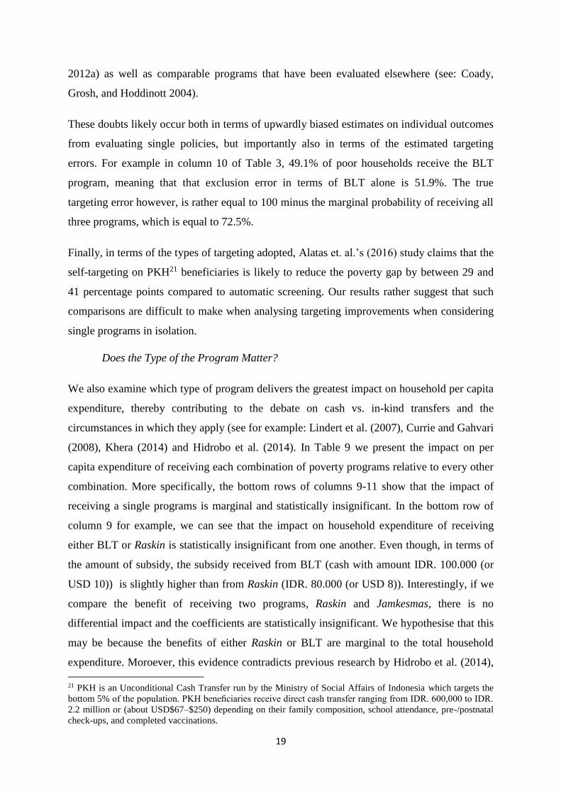
These doubts likely occur both in terms of upwardly biased estimates on individual outcomes

from evaluating single policies, but importantly also in terms of the estimated targeting

errors. For example in column 10 of Table 3, 49.1% of poor households receive the BLT

program, meaning that that exclusion error in terms of BLT alone is 51.9%. The true

targeting error however, is rather equal to 100 minus the marginal probability of receiving all

three programs, which is equal to 72.5%.

Finally, in terms of the types of targeting adopted, Alatas et. al.’s (2016) study claims that the

self-targeting on PKH21 beneficiaries is likely to reduce the poverty gap by between 29 and

41 percentage points compared to automatic screening. Our results rather suggest that such

comparisons are difficult to make when analysing targeting improvements when considering

single programs in isolation.

Does the Type of the Program Matter?

We also examine which type of program delivers the greatest impact on household per capita

expenditure, thereby contributing to the debate on cash vs. in-kind transfers and the

circumstances in which they apply (see for example: Lindert et al. (2007), Currie and Gahvari

(2008), Khera (2014) and Hidrobo et al. (2014). In Table 9 we present the impact on per

capita expenditure of receiving each combination of poverty programs relative to every other

combination. More specifically, the bottom rows of columns 9-11 show that the impact of

receiving a single programs is marginal and statistically insignificant. In the bottom row of

column 9 for example, we can see that the impact on household expenditure of receiving

either BLT or Raskin is statistically insignificant from one another. Even though, in terms of

the amount of subsidy, the subsidy received from BLT (cash with amount IDR. 100.000 (or

USD 10)) is slightly higher than from Raskin (IDR. 80.000 (or USD 8)). Interestingly, if we

compare the benefit of receiving two programs, Raskin and Jamkesmas, there is no

differential impact and the coefficients are statistically insignificant. We hypothesise that this

may be because the benefits of either Raskin or BLT are marginal to the total household

expenditure. Moroever, this evidence contradicts previous research by Hidrobo et al. (2014),

21 PKH is an Unconditional Cash Transfer run by the Ministry of Social Affairs of Indonesia which targets the

bottom 5% of the population. PKH beneficiaries receive direct cash transfer ranging from IDR. 600,000 to IDR.

2.2 million or (about USD$67–$250) depending on their family composition, school attendance, pre-/postnatal

check-ups, and completed vaccinations.

20

who claim that cash is preferable if the objective of the transfers are to improve household

welfare.

Conclusion

Social programs aimed at targeting poverty constitute crucial welfare interventions designed

to improve the welfare of poor households. The evaluation of these programs however, have

been stymied by the fact that they are evaluated in isolation, which may result in serious

upward biases due to individuals’ outcomes being primarily driven by omitted programs. In

this paper, we combine unique proxy means testing administrative data and survey data from

various sources pertaining to the three largest social programs in Indonesia, accounting for

more than 80% of total social expenditure, to evaluate the nationwide impact of program

complementarities on household expenditure and poverty reduction. Our evaluation takes

place before and after the introduction of Indonesia’s Unified Targeting system, which was

introduced to reduce targeting errors while increasing complementarities between programs.

Our results show that the introduction of the Unified Targeting system more than doubled the

proportion of households that benefited from all three social programs.

To evaluate the role of complementarities on household expenditure and poverty, we

introduce a new method of evaluation. Exploiting the design of all three poverty programs,

we then estimate the impact of targeting under the condition of multiple programs and show

that households that receive all three programs are at least 30 percentage points better off

than those that receive none. We further provide evidence that the level of bias from failing to

account for program complementarities, of between 16 and 19 percentage points, is greater in

magnitude than the benefits of receiving a single program, thereby demonstrating the clear

need to account for program complementarities. Further speaking to the cash vs. in-kind

transfer debate, we show in the context of Indonesia that the type of program has no

discernible effect on household welfare or poverty.

21

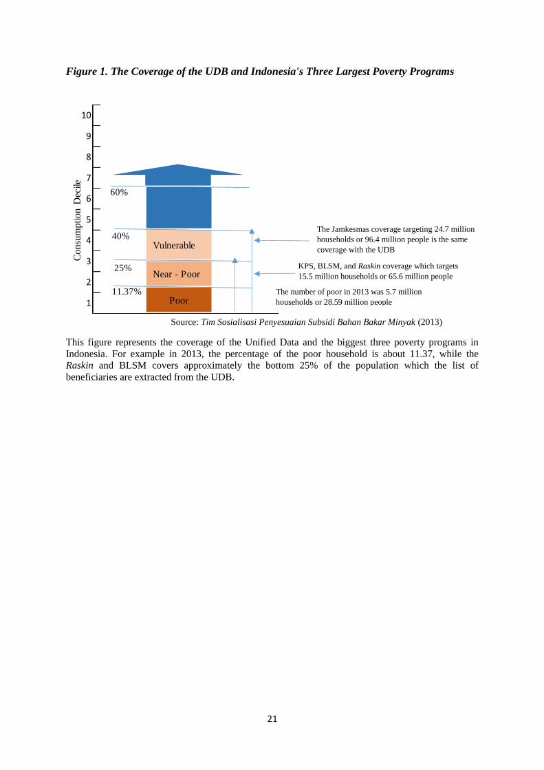
Figure 1. The Coverage of the UDB and Indonesia's Three Largest Poverty Programs

This figure represents the coverage of the Unified Data and the biggest three poverty programs in

Indonesia. For example in 2013, the percentage of the poor household is about 11.37, while the

Raskin and BLSM covers approximately the bottom 25% of the population which the list of

beneficiaries are extracted from the UDB.

4

3

2

1

10

9

8

7

6

5

Poor

Near - Poor

Vulnerable

11.37%

25%

40%

60%

Consu

mption D

ecile

The number of poor in 2013 was 5.7 million

households or 28.59 million people

KPS, BLSM, and Raskin coverage which targets

15.5 million households or 65.6 million people

The Jamkesmas coverage targeting 24.7 million

households or 96.4 million people is the same

coverage with the UDB

Source: Tim Sosialisasi Penyesuaian Subsidi Bahan Bakar Minyak (2013)

22

Figure 2. Third Generation of Social Protection Programs and Development of the UDB

This figure presents the time line of the introduction of the third generation of social protection in Indonesia

which was started by the development of the UDB in 2012. The list of households in the UDB was constructed

using the PPLS 2011 dataset and rank using PMT with 482 unique cut-offs for each district.

Source: Authors’ tabulation from multiple sources of the GoI official documents such as the guideline of

SUSENAS Survey, Population Census, Podes, and others. Note: the blue dots denote the periods of SUSENAS

survey

23

Figure 3. Time Horizon of Data Collection in the Periods between 2013 and 2014

This figure shows the time line of data collections which are utilized in this study. This study use unique

dataset that was collected specifically for the evaluation of poverty targeting and the delivery of poverty

programs in Indonesia, namely the SPS (for Survei Perlindungan Sosial or Social Protection Survey) which is

combined with Official PMT coefficient used by the GoI in selecting the beneficiaries of each poverty

programs and other dataset (e.g. PODES and SUSENAS).

Source: Author tabulation from multiple sources of the GoI official documents such as the guideline of

SUSENAS Survey, Social Protection Survey, Podes, and others. Note: The blue dotes denote the periods of

SUSENAS survey.

24

Figure 4. Estimation of Propensity Score based on PMT Score and Underlying

Covariates

A B

This figure presents the overlap of Propensity Score (�̂�). The panel A is estimated using PMT score

as a single covariate. While the panel B is estimated using underlying covariates as presented in Table

A3 in the appendix.

Figure 5. Baseline of PMT score across treatment level

‘None’ is the distribution of households that did not receive any poverty programs, while ‘one’,

‘two’, or ‘three’ rather denote how many poverty programs were received by households. ‘None,

reweighted’, is the distribution of households that received nothing adjusted by the inverse

probability weights, �̂�.

25

Table 1 Targeting Matrix of the Complementary Multiple Programs

Poverty Status Total

Poor Non-poor

Beneficiaries status of

program BLT

Beneficiary Correct of inclusion (𝐶1𝐵) Error of Inclusion (𝐸1𝐵) 𝐵𝐵

Non- beneficiary Error of Exclusion (𝐸2𝐵) Correct Exclusion (𝐶2𝐵) 𝑁𝐵𝐵

Beneficiaries status of

program Raskin

Beneficiary Correct of inclusion (𝐶1𝑅) Error of Inclusion (𝐸1𝑅) 𝐵𝑅

Non- beneficiary Error of Exclusion (𝐸2𝑅) Correct Exclusion (𝐶2𝑅) 𝑁𝐵𝑅

Beneficiaries status of

program Jamkesmas

Beneficiary Correct of inclusion (𝐶1𝐽) Error of Inclusion (𝐸1𝐽) 𝐵𝐽

Non- beneficiary Error of Exclusion (𝐸2𝐽) Correct Exclusion (𝐶2𝐽) 𝑁𝐵𝐽

P NP T

This table represent an extension of the standard matrix used in evaluation the performance of poverty

targeting. The information about the standard matrix can be found in studies by Coady, Grosh, and

Hoddinott, (2004).

Table 2. Joint and marginal probabilities of poor households receiving poverty

programs

Joint

probability

Marginal

(BLT)

Marginal

(Raskin)

Marginal

(Jamkesmas) Total

(1) (2) (3) (4) (5)

BLT only (𝐶𝐵=1,𝑅=0,𝐽=0/𝑃) (𝐶𝐵=1,𝑅=0,𝐽=0/𝑃) - -

Raskin only (𝐶𝐵=0,𝑅=1,𝐽=0/𝑃) - (𝐶𝐵=0,𝑅=1,𝐽=0/𝑃) -

Jamkesmas only (𝐶𝐵=0,𝑅=0,𝐽=1/𝑃) - - (𝐶𝐵=0,𝑅=0,𝐽=1/𝑃)

BLT and Raskin only (𝐶𝐵=1,𝑅=1,𝐽=0/𝑃) (𝐶𝐵=1,𝑅=1,𝐽=0/𝑃) (𝐶𝐵=1,𝑅=1,𝐽=0/𝑃)

BLT and Jamkesmas only (𝐶𝐵=1,𝐽=1,𝑅=0/𝑃) (𝐶𝐵=1,𝐽=1,𝑅=0/𝑃) - (𝐶𝐵=1,𝐽=1,𝑅=0/𝑃)

Raskin and Jamkesmas only (𝐶𝑅=1,𝐽=1,𝐵=0/𝑃) - (𝐶𝑅=1,𝐽=1,𝐵=0/𝑃) (𝐶𝑅=1,𝐽=1,𝐵=0/𝑃)

BLT, Raskin and Jamkesmas (𝐶𝐵=1,𝑅=1,𝐽=1/𝑃) (𝐶𝐵=1,𝑅=1,𝐽=1/𝑃) (𝐶𝐵=1,𝑅=1,𝐽=1/𝑃) (𝐶𝐵=1,𝑅=1,𝐽=1/𝑃)

None (𝐶𝐵=0,𝑅=0,𝐽=0/𝑃) - - - 𝑒𝑒𝑇

Total 100 𝐶1𝐵/𝑃 𝐶1𝑅/𝑃 𝐶1𝐽/𝑃

This table is constructed using information from Table 1 to measure the degree of complementarity of

each program with respect to the others. For example, under perfect complementarities, the joint

probability of poor households receiving three programs will be equal to the total marginal probability

for all programs. This implies that under this condition, the joint probability for poor households

receiving either one or two programs will be zero.

26

Table 3 Observed joint and marginal probabilities of the poor household receiving the poverty programs

Targeting Methods → 2005a 2009a 2014b

Probabilities → Joint

Marginal Joint

Marginal Joint

Marginal

Programs ↓ BLT Raskin Jamkesmas BLT Raskin Jamkesmas BLT Raskin Jamkesmas

(1) (2) (3) (4) (5) (6) (7) (8) (9) (10) (11) (12)

BLT only 7.89 7.89

4.76 4.76

3.96 3.96

Raskin only 18.28

18.28

23.74

23.74

19.66

19.66

Jamkesmas only 0.93

0.93 1.55

1.55 4.49

4.49

BLT and Raskin only 30.96 30.96 30.96

24.78 24.78 24.78

9.42 9.42 9.42

BLT and Jamkesmas only 1.73 1.73

1.73 1.61 1.61

1.61 8.21 8.21

8.21

Raskin and Jamkesmas only 2.93

2.93 2.93 3.53

3.53 3.53 9.20

9.20 9.20

BLT, Raskin and Jamkesmas 15.66 15.66 15.66 15.66 12.67 12.67 12.67 12.67 27.51 27.51 27.51 27.51

None 21.62

27.36

17.55

Total 100.00 56.24 67.83 21.25 100.00 43.82 64.72 19.36 100.00 49.10 65.79 49.41

This table present the joint and marginal probability of poor households receiving either one, two or the program which is measured using the formula

presented in Table 2. Source: Authors’ calculation. Note: a) are measured using SUSENAS 2006 and 2009; b) is measured using SUSENAS and Social

Protection Survey (SPS) 2014.

27

Table 4 Observed conditional and unconditional probabilities of poor households receiving poverty programs based on different

targeting methods

Targeting Methods → 2005a 2009a 2014b

Probabilities → BLT Raskin Jamkesmas BLT Raskin Jamkesmas BLT Raskin Jamkesmas

Programs ↓ (1) (2) (3) (4) (5) (6) (7) (8) (9)

P(.) 56.24 67.83 21.25 43.82 64.72 19.36 49.10 65.79 49.41

P(. |BLT = 1) 100.00 82.89 30.92 100.00 85.46 32.59 100.00 75.21 72.75

P(. |Raskin = 1) 68.73 100.00 27.41 57.86 100.00 25.03 56.13 100.00 55.80

P(. |Jamkesmas = 1) 81.84 87.48 100.00 73.76 83.68 100.00 72.29 74.30 100.00

P(. |Raskin = 1, Jamkesmas = 1) 84.24 100.00 100.00 78.21 100.00 100.00 74.94 100.00 100.00

P(. |BLT = 1, Jamkesmas = 1) 100.00 90.05 100.00 100.00 88.73 100.00 100.00 77.02 100.00

P(. |BLT = 1, Raskin = 1) 100.00 100.00 33.59 100.00 100.00 33.83 100.00 100.00 74.49

This table presents conditional and unconditional probabilities measured based on information in Table 3. The number on each cell of the table is derived

using formula presented in either Equation (1), 2, 3, or 4 depending its condition. Note: a) are measured using SUSENAS 2006 and 2009; b) is measured

using SUSENAS and Social Protection Survey (SPS) 2014.

28

Table 5. Observed joint and marginal probabilities of the poor household receiving the poverty programs in 2014 (with or without KPS)

Years → Poor Households - All Sample Poor Households - with KPS Poor Households - without KPS

Probabilities → Joint

Marginal Probabilities Joint

Marginal Probabilities Joint

Marginal Probabilities

Programs ↓ BLT Raskin Jamkesmas BLT Raskin Jamkesmas BLT Raskin Jamkesmas

(1) (2) (3) (4) (5) (6) (7) (8) (9) (10) (11) (12)

BLT only 3.96 3.96

6.52 6.52

1.89 1.89

Raskin only 19.66

19.66

0.67

0.67

35.02

35.02

Jamkesmas only 4.49

4.49 1.20

1.20 7.14

7.14

BLT and Raskin only 9.42 9.42 9.42

16.62 16.62 16.62

3.60 3.60 3.60

BLT and Jamkesmas only 8.21 8.21

8.21 16.32 16.32

16.32 1.65 1.65

1.65

Raskin and Jamkesmas only 9.20

9.20 9.20 1.44

1.44 1.44 15.48

15.48 15.48

BLT, Raskin and Jamkesmas 27.51 27.51 27.51 27.51 56.79 56.79 56.79 56.79 3.83 3.83 3.83 3.83

None 17.55

0.44

31.39

Total 100.00 49.10 65.79 49.41 100.00 96.25 75.52 75.75 100.00 10.97 57.93 28.10

This Table present probabilities measured as in Table 4 with dividing the sample becomes either the households received KPS or did not. Note: This

probabilities are measured using SUSENAS and Social Protection Survey (SPS) 2014.

29

Table 6. Observed conditional and unconditional probabilities of the poor household receiving the poverty programs in 2014 (with or

without KPS)

Years → Poor Households - All Sample Poor Households - with KPS Poor Households - without KPS

Probabilities → BLT Raskin Jamkesmas BLT Raskin Jamkesmas BLT Raskin Jamkesmas

Programs ↓ (1) (2) (3) (4) (5) (6) (7) (8) (9)

P(.) 49.10 65.79 49.41 96.25 75.52 75.75 10.97 57.93 28.10

P(. |BLT = 1) 100.00 75.21 72.75 100.00 76.27 75.96 100.00 67.73 49.95

P(. |Raskin = 1) 56.13 100.00 55.80 97.21 100.00 77.11 12.83 100.00 33.33

P(. |Jamkesmas = 1) 72.29 74.30 100.00 96.51 76.87 100.00 19.50 68.72 100.00

P(. |Raskin = 1, Jamkesmas = 1) 74.94 100.00 100.00 97.53 100.00 100.00 19.83 100.00 100.00

P(. |BLT = 1, Jamkesmas = 1) 100.00 77.02 100.00 100.00 77.68 100.00 100.00 69.89 100.00

P(. |BLT = 1, Raskin = 1) 100.00 100.00 74.49 100.00 100.00 77.36 100.00 100.00 51.55

This table present probabilities measured as in Table 5 with dividing the sample becomes either the households received KPS or did not. This probabilities are

measured using SUSENAS and Social Protection Survey (SPS) 2014.

30

Table 7 Difference on Per Capita Expenditure

OLS IPW Double Robustness Control

Function Estimator

(1) (2) (3) (4) (5)

3 Programs vs. None

0.085 0.085 0.126 0.126 0.143

(0.012)*** (0.012)*** (0.012)*** (0.012)*** (0.012)***

-0.248 -0.284 -0.274 -0.274 -0.190

(0.009)*** (0.010)*** (0.009)*** (0.009)*** (0.011)***

0.333 0.369 0.400 0.400 0.332

(0.013)*** (0.014)*** (0.013)*** (0.014)*** (0.013)***

Reweighted No Yes Yes Yes

Yes

Propensity Score Control No No Yes No Yes

PMT score control No No No Yes No

Number of Households 63,681 67,118 67,118 67,118 67,118

0.154 0.159 0.178 0.178 0.184

2 Programs vs. None

0.036 0.034 0.053 0.052 0.058

(0.010)*** (0.010)*** (0.011)*** (0.011)*** (0.011)***

-0.256 -0.293 -0.287 -0.287 -0.204

(0.009)*** (0.009)*** (0.010)*** (0.009)*** (0.012)***

0.292 0.327 0.340 0.339 0.262

(0.011)*** (0.012)*** (0.013)*** (0.013)*** (0.013)***

Reweighted No Yes Yes Yes

Yes

Propensity Score Control No No Yes No Yes

PMT score control No No No Yes No

Number of Households 63,681 67,118 67,118 67,118 67,118

0.153 0.158 0.177 0.176 0.182

1 Program vs. None

-0.068 -0.064 -0.104 -0.105 -0.130

(0.010)*** (0.010)*** (0.011)*** (0.010)*** (0.010)***

-0.300 -0.334 -0.353 -0.352 -0.276

(0.010)*** (0.011)*** (0.012)*** (0.012)*** (0.012)***

0.232 0.270 0.248 0.248 0.146

(0.009)*** (0.010)*** (0.010)*** (0.010)*** (0.012)***

Reweighted No Yes Yes Yes

Yes

Propensity Score Control No No Yes No Yes

PMT score control No No No Yes No

Number of Households 63,681 67,118 67,118 67,118 67,118

0.154 0.159 0.179 0.178 0.185

Notes: the dependent variable is the difference log total per capita expenditure between before and

after treatment. The first column denotes the pure OLS estimation, while the next column is the

results of IPW estimator. Column 3 and 4 are the double robustness estimation which is proposed by

Scharfstein et al. (1999), and column 5 is the five-subclass estimation following Rosenbaum and

Rubin (1984). The standard errors (presented in parentheses) in column 2-5 are clustered by the

village and computed over the entire two-step using a block bootstrap with 500 repetitions following

Cameron et. al, 2008. *** p<0.01, ** p<0.05, * p<0.1.

(�̂�ℎ) (𝑃𝑀𝑇ℎ)

𝜽𝟑

𝜽𝟎

𝜽𝟑𝟎

= 𝜽𝟑 − 𝜽𝟎

𝑹𝟐

𝜽𝟐

𝜽𝟎

𝜽𝟐𝟎

= 𝜽𝟐 − 𝜽𝟎

𝑹𝟐

𝑹𝟐

𝜽𝟏

𝜽𝟎

𝜽𝟏𝟎

= 𝜽𝟏 − 𝜽𝟎

31

Table 8 Difference on Poverty Gap Index (FGT)

OLS IPW Double Robustness

Control

Function Estimator

(1) (2) (3) (4) (5)

3 Programs vs. None

-0.017 -0.017 -0.010 -0.009 -0.009

(0.002)*** (0.002)*** (0.002)*** (0.002)*** (0.002)***

0.019 0.007 0.008 0.008 0.026

(0.001)*** (0.001)*** (0.001)*** (0.001)*** (0.002)***

-0.0358 -0.023 -0.018 -0.018 -0.035

(0.001)*** (0.002)*** (0.002)*** (0.002)*** (0.002)***

Reweighted No Yes Yes Yes

Yes

Propensity Score Control No No Yes No Yes

PMT score control No No No Yes No

Number of Households 63,681 67,118 67,118 67,118 67,118

0.057 0.0561 0.103 0.107 0.112

2 Programs vs. None

-0.010 -0.008 -0.005 -0.005 -0.006

(0.001)*** (0.002)*** (0.002)*** (0.002)*** (0.001)***

0.020 0.008 0.009 0.009 0.027

(0.001)*** (0.001)*** (0.001)*** (0.001)*** (0.002)***

-0.0298 -0.016 -0.014 -0.014 -0.032

(0.001)*** (0.002)*** (0.002)*** (0.002)*** (0.002)***

Reweighted No Yes Yes Yes

Yes

Propensity Score Control No No Yes No Yes

PMT score control No No No Yes No

Number of Households 63,681 67,118 67,118 67,118 67,118

0.054 0.0538 0.103 0.106 0.112

1 Programs vs. None

0.018 0.018 0.011 0.010 0.009

(0.001)*** (0.001)*** (0.001)*** (0.001)*** (0.001)***

0.031 0.019 0.016 0.015 0.032

(0.001)*** (0.002)*** (0.002)*** (0.002)*** (0.002)***

-0.0137 -0.001 -0.005 -0.005 -0.023

(0.001)*** (0.001) (0.001)*** (0.001)*** (0.002)***

Reweighted No Yes Yes Yes

Yes

Propensity Score Control No No Yes No Yes

PMT score control No No No Yes No

Number of Households 63,681 67,118 67,118 67,118 67,118

0.060 0.0589 0.104 0.108 0.113

Notes: the dependent variable is the difference of Poverty Gap Index (FGT1) between 2011 and

March 2014. All conditions used in the estimation can be seen in Table 11. *** p<0.01, ** p<0.05, *

p<0.1.

𝜽𝟑𝟑

𝜽𝟎𝟎

𝜽𝟑𝟎

= 𝜽𝟑𝟑 − 𝜽𝟎𝟎

𝑹𝟐

(�̂�ℎ) (𝑃𝑀𝑇ℎ)

𝜽𝟐𝟑

𝜽𝟎𝟎

𝜽𝟐𝟎

= 𝜽𝟐𝟑 − 𝜽𝟎𝟎

𝑹𝟐

𝜽𝟏𝟑

𝜽𝟎𝟎

𝜽𝟏𝟎

= 𝜽𝟏𝟑 − 𝜽𝟎𝟎

𝑹𝟐

32

Table 9 Matrix Comparison – Combination between Treatments and Controls using Control Function Estimation

None 3 Programs 2 Program 1 Program BLT and

Raskin only

BLT and

Jamkesmas

only

Raskin and

Jamkesmas

only

BLT

only

Raskin

only

Jamkesmas

only

(1) (2) (3) (4) (5) (6) (7) (8) (9) (10) (11)

None 0.316 0.247 0.128 0.245 0.274 0.232 0.162 0.129 0.136

(0.014)*** (0.012)*** (0.011)*** (0.019)*** (0.020)*** (0.016)*** (0.038)*** (0.012)*** (0.019)***

3 Programs 0.316 0.0731 0.184 0.0709 0.0395 0.0896 0.160 0.185 0.189

(0.014)*** (0.013)*** (0.013)*** (0.020)*** (0.022)*** (0.016)*** (0.040)*** (0.013)*** (0.021)***

2 Programs 0.247 0.0731 0.110 0.0820 0.112 0.111

(0.012)*** (0.013)*** (0.011)*** (0.039)** (0.012)*** (0.020)***

1 Programs 0.128 0.184 0.110 0.112 0.145 0.0920

(0.011)*** (0.013)*** (0.011)*** (0.019)*** (0.020)*** (0.014)***

BLT and Raskin only 0.245 0.0709 0.112 0.0514 0.0185 0.0837 0.114 0.114

(0.019)*** (0.020)*** (0.019)*** (0.023)** (0.022) (0.041)** (0.019)*** (0.025)***

BLT and Jamkesmas only 0.274 0.0395 0.145 0.0514 0.0329 0.117 0.148 0.143

(0.020)*** (0.022)*** (0.020)*** (0.023)** (0.026) (0.042)*** (0.021)*** (0.024)***

Raskin and Jamkesmas only 0.232 0.0896 0.0920 0.0185 0.0329 0.068 0.093 0.095

(0.016)*** (0.016)*** (0.014)*** (0.022) (0.026) (0.041)* (0.015)*** (0.023)***

BLT only 0.162 0.160 0.0820 0.0837 0.117 0.068 0.029 0.028

(0.038)*** (0.040)*** (0.039)** (0.041)** (0.042)*** (0.041)* (0.039) (0.042)

Raskin only 0.129 0.185 0.112 0.114 0.148 0.093 0.029 0.000

(0.012)*** (0.013)*** (0.012)*** (0.019)*** (0.021)*** (0.015)*** (0.039) (0.020)

Jamkesmas only 0.136 0.189 0.111 0.114 0.143 0.095 0.028 0.000

(0.019)*** (0.021)*** (0.020)*** (0.025)*** (0.024)*** (0.023)*** (0.042) (0.020)

Notes: the dependent variable is the difference log total per capita expenditure between before and after treatment. All estimations are conducted under five-subclass estimation following

Rosenbaum and Rubin (1984). *** p<0.01, ** p<0.05, * p<0.1.

33

References

Abadie, A. (2005). Semiparametric difference-in-differences estimators. The Review of Economic

Studies, 72(1), 1-19.

Alatas, V., et al. (2016). "Self-Targeting: Evidence from a Field Experiment in Indonesia." Journal of

Political Economy 124(2): 371-427.

Alatas, V., et al. (2012). "Targeting the Poor: Evidence from a Field Experiment in Indonesia." The

American Economic Review 102(4): 1206-1240.

Bah, A., Bazzi, S., Sumarto, S., and Tobias, J. (2014). Finding the Poor vs. Measuring Their Poverty:

Exploring the Drivers of Targeting Effectiveness in Indonesia. TNP2K Working Paper No. 20.

Banerjee, A., Hanna, R., Kyle, J., Olken, B. A., and Sumarto, S. (2015a). Tangible Information and

Citizen Empowerment: Identification Cards and Food Subsidy Programs in Indonesia.

Massachusetts Institute of Technology, 39.

Banerjee, A., et al. (2015b). A multifaceted program causes lasting progress for the very poor:

Evidence from six countries. Science, 348(6236), 1260799.

Bazzi, S., et al. (2015). "It's all in the timing: Cash transfers and consumption smoothing in a

developing country." Journal of Economic Behavior and Organization 119: 267-288.

Busso, M., DiNardo, J., and McCrary, J. (2014). New evidence on the finite sample properties of

propensity score reweighting and matching estimators. Review of Economics and Statistics,

96(5), 885-897.

Cameron, L. and M. Shah (2014). "Can Mistargeting Destroy Social Capital and Stimulate Crime?

Evidence from a Cash Transfer Program in Indonesia." Economic Development and Cultural

Change 62(2): 381-415.

Castaneda, T. and L. Fernandez (2005). "Targeting social spending to the poor with proxy-means

testing: Colombia’s SISBEN system." World Bank Human Development Network Social

Protection Unit Discussion Paper 529.

Coady, D., Grosh, M. E., and Hoddinott, J. (2004). Targeting of transfers in developing countries:

Review of lessons and experience (Vol. 1). World Bank Publications.

Currie, J., and Gahvari, F. (2008). Transfers in cash and in-kind: theory meets the data. Journal of

Economic Literature, 46(2), 333-383.

De la Brière, B. and K. Lindert (2005). "Reforming Brazil’s Cadastro Único to improve the targeting

of the Bolsa Família Program." World Bank, Social Protection Unit and DFID.

Grosh, M., et al. (2008). For protection and promotion: The design and implementation of effective

safety nets, World Bank Publications.

Hastuti, et al. (2006). A Rapid Appraisal of the Implementation of the 2005 Direct Cash Transfer

Program in Indonesia: A Case Study of Five Kabupaten/Kota. Jakarta, SMERU Research

Report.

34

Hidrobo, M., Hoddinott, J., Peterman, A., Margolies, A., and Moreira, V. (2014). Cash, food, or

vouchers? Evidence from a randomized experiment in northern Ecuador. Journal of

Development Economics, 107, 144-156.

Hirano, K., Imbens, G. W., and Ridder, G. (2003). Efficient estimation of average treatment effects

using the estimated propensity score. Econometrica, 71(4), 1161-1189.

Imbens, G. W., and Wooldridge, J. M. (2009). Recent developments in the econometrics of program

evaluation. Journal of economic literature, 47(1), 5-86.

Jalan, J., and Ravallion, M. (2003). Estimating the benefit incidence of an antipoverty program by

propensity-score matching. Journal of Business and Economic Statistics, 21(1), 19-30.

Jellema, J. R. and H. Noura (2012). Main report. Public expenditure review (PER) Washington, DC:

World Bank.

Khera, R. (2014). Cash vs. in-kind transfers: Indian data meets theory. Food Policy, 46, 116-128.

Lindert, K., Linder, A., Hobbs, J., and De la Brière, B. (2007). The nuts and bolts of Brazil’s Bolsa

Família Program: implementing conditional cash transfers in a decentralized context (Vol.

709). Social Protection Discussion Paper.

Lunceford, J. K., and Davidian, M. (2004). Stratification and weighting via the propensity score in

estimation of causal treatment effects: a comparative study. Statistics in medicine, 23(19),

2937-2960.

Olken, B. A. (2005). "Revealed community equivalence scales." Journal of Public Economics 89(2–

3): 545-566.

Priebe, J. (2014). "Official Poverty Measurement in Indonesia since 1984: A Methodological

Review." Bulletin of Indonesian Economic Studies 50(2): 185-205.

Pritchett, L., Suryahadi, A., and Sumarto, S. (2000). Quantifying vulnerability to poverty: A proposed

measure, applied to Indonesia (No. 2437). World Bank Publications.

Ravallion, M. (2007). Evaluating anti-poverty programs. Handbook of development economics, 4,

3787-3846.

Rosenbaum, P. R., and Rubin, D. B. (1983). The central role of the propensity score in observational

studies for causal effects. Biometrika, 41-55.

Rosenbaum, P. R., and Rubin, D. B. (1984). Reducing bias in observational studies using

subclassification on the propensity score. Journal of the American statistical Association,

79(387), 516-524.

Rosfadhila, M., Toyamah, N., Sulaksono, B., Devina, S., Sodo, R. J., and Syukri, M. (2011). A Rapid

Appraisal of the Implementation of the 2008 Direct Cash Transfer Program and Beneficiary

Assessment of the 2005 Direct Cash Transfer Program in Indonesia. SMERU Research

Institute.

35

Scharfstein, D. O., Rotnitzky, A., and Robins, J. M. (1999). Adjusting for nonignorable drop-out

using semiparametric nonresponse models. Journal of the American Statistical Association,

94(448), 1096-1120.

Smith, J. A., and Todd, P. E. (2005). Does matching overcome LaLonde's critique of nonexperimental

estimators?. Journal of econometrics, 125(1), 305-353.

Sparrow, R. (2008). "Targeting the poor in times of crisis: the Indonesian health card." Health policy

and planning 23(3): 188-199.

Sparrow, R., et al. (2013). "Social health insurance for the poor: Targeting and impact of Indonesia's

Askeskin programme." Social Science and Medicine 96: 264-271.

Sumarto, S. and Bazzi, S. (2011). "Social Protection in Indonesia: Past Experiences and Lessons for

the Future." Paper presented at the 2011 Annual Bank Conference on Development

Opportunities (ABCDE) jointly organized by the World Bank and OECD.

Sumarto, S., Suryahadi, A., and Pritchett, L. (2003). Safety nets or safety ropes? Dynamic benefit

incidence of two crisis programs in Indonesia. World Development, 31(7), 1257-1277.

Sumarto, S., Suryahadi, A., and Widyanti, W. (2002), ‘Designs and Implementation of the Indonesian

Social Safety Net Programs’, Developing Economis, 40(1), pp. 3-31.

Suryahadi, A., Widyanti, W., and Sumarto, S. (2003). Short‐term poverty dynamics in rural Indonesia

during the economic crisis. Journal of International Development, 15(2), 133-144.

Tim Sosialisasi Penyesuaian Subsidi Bahan Bakar Minyak (2013). Buku Pegangan Sosialisasi dan

Implementasi Program-Program Kompensasi Kebijakan Penyesuaian Subsidi Bahan Bakar

Minyak 2013 (The guidelines for the implementation of the 2013 compensation program for

Fuel Subsidy Reduction Compensation Program). K. W. P. RI. Jakarta: Sekretariat Wakil

Presiden.

TNP2K (2015). Indonesia's Unified Database for Social Protection Programmes - Management

Standard. Jakarta, Secretariat of the Vice President of the Republic of Indonesia.

Widianto, B. (2013). "The political economy of social protection reforms in Indonesia." Social

Protection in Developing Countries: Reforming Systems 2: 161.

Widjaja, M. (2009). An Economic and Social Review on Indonesian Direct Cash Transfer Program to

Poor Families Year 2005. the Association for Public Policy Analysis and Management

International Conference on Asian Social Protection in Comparative Perspective. Singapore.

World Bank. (2006). Making the New Indonesia Work for the Poor. Jakarta

World Bank (2012a). Targeting Poor and Vulnerable Households in Indonesia. Jakarta.

World Bank. (2012b). Protecting Poor and Vulnerable Households in Indonesia.

Yusuf, A. A., and Resosudarmo, B. P. (2008). Mitigating distributional impact of fuel pricing reform:

the Indonesian experience. ASEAN Economic Bulletin, 25(1), 32-47.

36

Appendixes

Table A1 Household Characteristics by Receiving Poverty Program

Non-Receiving

Program Receiving Program Difference

PMT Score 13.616 (0.43)

13.492 (0.352) -0.100*** [0.013]

Percapita Expenditure ('000) 913.84 (1034)

632.980 (529.81) -239707*** [24571]

Head of Household Characteristics

Male 0.858 (0.349)

0.842 (0.364) -0.012* [0.007]

Married 0.818 (0.386)

0.813 (0.390) -0.005 [0.007]

Age 47.676 (13.568)

48.811 (13.737) 0.789*** [0.179]

Education

Elementary 0.202 (0.401)

0.248 (0.432) 0.042*** [0.008]

Junior High 0.206 (0.405)

0.247 (0.431) 0.037*** [0.005]

Senior High & University 0.415 (0.493)

0.299 (0.458) -0.106*** [0.012]

Working Status: Employed 0.879 (0.326)

0.893 (0.310) 0.015*** [0.005]

Employment Sector:

Agriculture 0.362 (0.481)

0.457 (0.498) 0.098*** [0.010]

Mining & Quarrying 0.020 (0.139)

0.015 (0.122) -0.000 [0.002]

Processing Industry 0.063 (0.242)

0.068 (0.251) -0.001 [0.003]

Trading 0.128 (0.334)

0.112 (0.315) -0.016*** [0.004]

Construction/building 0.067 (0.249)

0.078 (0.268) 0.010** [0.004]

Hotel & Restaurant 0.013 (0.115)

0.009 (0.097) -0.004*** [0.001]

Transportation & ICT 0.050 (0.218)

0.047 (0.212) -0.002 [0.003]

Household Characteristics

Size (Person) 3.878 (1.725)

3.787 (1.687) -0.056** [0.021]

Dependency ratio 0.654 (0.649)

0.650 (0.651) -0.004 [0.010]

Number of Household Member: 0-4 yrs 0.336 (0.568)

0.334 (0.554) 0.003 [0.005]

Number of Household Member at School

Age

Elementary 0.527 (0.737)

0.471 (0.696) -0.043*** [0.010]

Junior High 0.218 (0.457)

0.201 (0.440) -0.013*** [0.004]

Senior High 0.160 (0.405)

0.138 (0.371) -0.019*** [0.003]

University 0.076 (0.308)

0.039 (0.217) -0.035*** [0.004]

Assets

Bicycle 0.327 (0.469)

0.321 (0.467) -0.030*** [0.008]

Gas ≥ 3 kg 0.148 (0.355)

0.043 (0.203) -0.091*** [0.010]

Refrigerator 0.445 (0.497)

0.298 (0.458) -0.128*** [0.014]

Motorcycle 0.671 (0.470)

0.627 (0.484) -0.041** [0.015]

Water Access

Branded/Recycled Bottle Water 0.290 (0.454)

0.163 (0.369) -0.106*** [0.011]

Pipe with Meter 0.121 (0.326)

0.094 (0.292) -0.025*** [0.008]

Terrestrial well/pump 0.119 (0.323)

0.143 (0.350) 0.012* [0.006]

Protected/Covered well 0.197 (0.398)

0.254 (0.435) 0.038*** [0.008]

Unprotected/Uncovered well 0.274 (0.446)

0.346 (0.476) 0.082*** [0.011]

From buying from other parties 0.444 (0.497)

0.312 (0.463) -0.115*** [0.009]

Housing

Own 0.799 (0.401)

0.864 (0.342) 0.049*** [0.006]

rent 0.036 (0.186)

0.015 (0.123) -0.017*** [0.002]

Lease 0.046 (0.210)

0.018 (0.131) -0.021*** [0.003]

Company House 0.024 (0.152)

0.006 (0.078) -0.015*** [0.003]

Others 0.096 (0.294)

0.096 (0.295) 0.004 [0.005]

Continued to the next page

37

Non-Receiving

Program Receiving Program Difference

Lighting Sources

PLN Electricity 450 W 0.784 (0.412) 0.759 (0.427) -0.030** [0.013]

PLN Electricity without Meter 0.104 (0.306) 0.120 (0.325) 0.008 [0.007]

Non-PLN Electricity 0.050 (0.218) 0.047 (0.212) 0.004 [0.005]

Non-Electricity 0.062 (0.241) 0.073 (0.261) 0.019*** [0.006]

Final disposal

Septic Tank 0.624 (0.484)

0.554 (0.497) -0.067*** [0.014]

Pit hole 0.118 (0.322)

0.147 (0.354) 0.026*** [0.008]

River/Lake/Sea 0.176 (0.380)

0.195 (0.396) 0.018** [0.007]

Beach/open field/farm 0.064 (0.245)

0.078 (0.269) 0.019*** [0.006]

Defecation facility use

Personal 0.715 (0.451)

0.657 (0.475) -0.053*** [0.016]

Mutual 0.285 (0.451)

0.343 (0.475) 0.053*** [0.016]

House Characteristics

Wall material: Concrete 0.624 (0.484)

0.597 (0.491) -0.057*** [0.017]

Wall material: Wood 0.376 (0.484)

0.403 (0.491) 0.057*** [0.017]

Roof Materials: Concrete 0.025 (0.156)

0.017 (0.127) -0.008*** [0.002]

Roof Materials: Roof Tile 0.370 (0.483)

0.477 (0.500) 0.007 [0.007]

Roof Materials: Iron Sheet/Asbeston 0.546 (0.498)

0.445 (0.497) -0.009 [0.008]

Roof Materials: Shingle/Fiber/Palm 0.059 (0.235)

0.061 (0.240) 0.011 [0.006]

Number of Households 50,043

17,075 67,118

This table present the mean tests of the characteristics of households who received the poverty program

and did not. Number inside the parentheses is the standard deviation, while inside the square brackets

denote the standard error. ***p<0.01, **p<0.05, * p<0.1.

Table A2 Village Characteristics by Receiving Poverty Program

Non-Receiving

Program Receiving Program Difference

Village Characteristics

Rural area 0.650 0.477 0.819 0.385 0.142*** [0.011]

Distance to the nearest

Market (Km) 6.968 16.655 7.587 17.647 1.259** [0.583]

Health Facility (Km) 5.098 11.853 6.168 13.250 1.318*** [0.311]

Sub-district office (Km) 6.261 25.432 6.803 20.573 0.699 [0.438]

District office (Km) 29.843 53.452 34.582 47.342 6.132*** [1.708]

Village has:

Shophouse 0.340 0.474 0.223 0.416 -0.117*** [0.011]

Hotel 0.152 0.359 0.074 0.262 -0.065*** [0.007]

Cooperation 0.525 0.499 0.472 0.499 -0.062*** [0.009]

Credit Finance 0.502 0.500 0.496 0.500 -0.025*** [0.008]

Access to the Bank 0.297 0.457 0.180 0.384 -0.105*** [0.010]

School building

Elementary 0.947 0.224 0.947 0.223 -0.002 [0.003]

Junior High School 0.609 0.488 0.552 0.497 -0.054*** [0.008]

Senior High School 0.435 0.496 0.332 0.471 -0.095*** [0.008]

Village Health Facility (Polindes) 0.460 0.498 0.519 0.500 0.034*** [0.009]

Sub-Vil. Health Facility (Posyandu) 0.978 0.147 0.977 0.151 -0.003 [0.003]

Continued to the next page

38

Non-Receiving

Program Receiving Program Difference

Asphalt Road 0.782 0.413 0.730 0.444 -0.060*** [0.010]

Road can be accessed 4-wheel car 0.929 0.257 0.913 0.282 -0.026*** [0.008]

Head of Village Characteristics

Gender: Male 0.910 0.286 0.933 0.250 0.019*** [0.004]

Age (years old) 44.067 10.150 44.321 9.507 0.019 [0.176]

Education background

No Education 0.014 0.116 0.019 0.135 0.005** [0.002]

Elementary 0.017 0.128 0.018 0.133 0.002 [0.002]

Junior High School 0.101 0.302 0.137 0.344 0.032*** [0.007]

Senior High School 0.456 0.498 0.512 0.500 0.051*** [0.010]

University 0.040 0.196 0.044 0.204 0.001 [0.003]

Number of Households 50043 17075 67,118

This table present the mean tests of the village characteristics where the households who received the

poverty program and did not. Number inside the parentheses is the standard deviation, while inside the

square brackets denote the standard error. ***p<0.01, **p<0.05, * p<0.1.

Table A3 Underlying Variables of PMT Score

dy/dx (S.E)

dy/dx (S.E)

Head of HHD: Male -0.099 (0.014)***

Primary income source (reference = other)

Married Status Head of HHD 0.042 (0.012)***

Head of HHD working -0.017 (0.014)

h_hhsize 0.058 (0.004)***

Agriculture 0.111 (0.016)***

Age of Head of HHD 0.000 (0.001)

Mining and Quarrying 0.092 (0.034)***

# HHD member 0-4 years -0.021 (0.009)**

Processing Industry 0.110 (0.023)***

Dependency Ratio 0.008 (0.007)

Trading 0.060 (0.015)***

Construction/building 0.189 (0.016)***

Household head education level (reference = No

education)

Hotel and Restaurant 0.011 (0.028)

Elementary -0.073 (0.010)***

Transportation and warehousing 0.115 (0.016)***

Junior High -0.126 (0.017)***

Public service 0.054 (0.012)***

High School - S3 -0.291 (0.022)***

Self-Owned business 0.014 (0.009)

Highest Education Background in the Household

(reference: No education)

Self-Owned business with non-

permanent worker -0.013 (0.011)

Elementary 0.056 (0.011)***

Self-Owned business with

permanent worker -0.124 (0.020)***

Junior High 0.056 (0.009)***

Senior High - S3 -0.059 (0.010)***

Home ownership Status (reference = Other)

Own -0.019 (0.014)

Number of Household members who are studying at: rent -0.207 (0.038)***

Elementary 0.000 (0.005) Lease -0.279 (0.033)***

Junior High 0.002 (0.007) Company House -0.332 (0.073)***

Senior High -0.024 (0.009)**

University -0.063 (0.014)*** Source of Ligthing (Reference = No Electricity)

Source of Lighting: 0.059 (0.040)

PLN Electricity without Meter 0.124 (0.042)***

Non-PLN Electricity 0.002 (0.030)

Continued to the next page

39

dy/dx (S.E)

dy/dx (S.E)

Household Assets:

Final Disposal Location (Reference = Other)

Bicycle 0.004 (0.008)

Septic Tank -0.060 (0.026)**

gas >= 12 kg -0.262 (0.019)***

River/Lake/Sea -0.015 (0.028)

Refrigerator -0.164 (0.014)***

Pit hole -0.032 (0.024)

Motorcycle -0.092 (0.011)***

Beach/open field/farm -0.038 (0.026)

River/Lake/Sea -0.015 (0.028)

Source of Drinking Water (reference = Unprotected well)

Pit hole -0.032 (0.024)

Branded/Recycled Bottle Water -0.124 (0.016)***

Beach/open field/farm -0.038 (0.026)

Pipe with Meter -0.065 (0.024)***

Terrestrial well/pump -0.027 (0.018)

Defecation facility use (Reference = mutual)

Protected/Covered well 0.005 (0.014)

Personal -0.083 (0.013)***

Buying 0.007 (0.011)

Type of wall material (reference = wood)

Roof Materials (Reference = Shingle/Fiber/Palm)

Type of wall material: Concrete -0.099 (0.010)***

Concrete -0.073 (0.037)**

Roof Tile -0.013 (0.043)

Type of flooring material: Not Soil -0.076 (0.056)

Iron Sheet/Asbeston -0.027 (0.032)

Pseudo R2 0.2953

Households 67,118

This table presents the marginal effect of Probit estimation. The dependent variable is 1 if the household

receive any poverty programs, 0 otherwise. Standard errors in parentheses. *** p<0.01, ** p<0.05,

*p<0.1.

Figure A1 The Evolution of the Social Protection Programs in Indonesia: The First and Second Generations