Distributive laws for the

Coinductive Solution of Recursive Equations

Bart Jacobs

Institute for Computing and Information Sciences,

Radboud University Nijmegen

P.O. Box 9010, 6500 GL Nijmegen, The Netherlands

Email: B.Jacobs@cs.ru.nl URL: http://www.cs.ru.nl/B.Jacobs

Abstract

This paper illustrates the relevance of distributive laws for the solution of recursiveequations, and shows that one approach for obtaining coinductive solutions of equa-tions via infinite terms is in fact a special case of a more general approach using anextended form of coinduction via distributive laws.

1 Introduction

Distribution x(y + z) = xy + xz is common in many equational theories, suchas vector spaces. It may also occur in so-called distributive categories, of theform X × (Y + Z) ∼= (X × Y ) + (X × Z), see e.g. [8], where one directionof the isomorphism is canonical and always exists. More generally, one canhave distributions GF ⇒ FG between two endofunctors F,G on the samecategory, as first studied in [7]. This phenomenon is especially interestingwhen the functors F,G form signatures (or interfaces) for certain operations,either in algebraic or in coalgebraic form.

Turi and Plotkin [25] first investigated such a situation where one functorG describes the syntax of a programming language and the other functor Fthe behaviour of programs (terms) in that language. Having a distributivelaw GF ⇒ FG means that the behaviour on terms is well-defined, and leadsto results like: (coalgebraic) bisimilarity is an (algebraic) congruence. Hencedistributive laws capture where “algebra meets coalgebra”.

The theme of this paper is the same, in a slightly different context, namelyrecursive equations xi = ti(x1, . . . , xn). The ti are terms from some algebra,and may contain the recursive variables xj. The solutions of such equations

Preprint submitted to Elsevier Preprint 18th March 2005

are typically infinite, and are thus best described via (final) coalgebras. Hencealso in this situation algebra and coalgebra meet, and appropriate distributivelaws are to be expected.

The finality principle in the theory of coalgebras is usually called coinduc-tion [15]. It involves the existence and uniqueness of suitable coalgebra homo-morphisms to final coalgebras. It was realised early on (see [1,6]) that suchcoinductively obtained homomorphisms can be understood as solutions to re-cursive (or corecursive, if you like) equations. The equation itself is incorpo-rated in the commuting square expressing that there is a homomorphism froma certain “source” coalgebra to the final coalgebra. Since this diagram arisesfrom the source coalgebra, this source can also be identified with the recursiveequation (see Section 3 for examples).

A systematic investigation of the solution of such equations first appeared in[20], followed by [2]. Their coalgebraic approach simplifies results for recursiveequations with infinite terms from [10,11]. More recently, a general and ab-stract approach is proposed in [5], using distributive laws. It builds on earlierwork [17] and may also be described dually, for algebras, as developed inde-pendently in [26]. One of the main contributions of this paper is that it showshow the approach of [2] for infinite terms fits in the general approach of [5]with distributive laws. This involves the identification of suitable distributivelaws of the monads of terms over the underlying interface functor.

This paper is organised as follows. Section 2 briefly reviews the approachof [5] based on distributive laws. It is illustrated in the context of languagesand automata in Section 3. Section 4 continues with two distributive laws forcanonical monads F ∗ and F∞ associated with a functor F . The approach of [2]for solutions of equations with infinite terms is then explained in Section 5.Finally, Section 6 shows that this approach is an instance of the distribution-based approach.

An earlier version of this paper appeared as [12]. The present version ex-tends [12] especially with Section 3 on distributive laws for languages andautomata. This topic is further elaborated in [14].

2 Distributive laws and solutions of equations

Distributive laws found their first serious application in the area of coalgebrasin the work of Turi and Plotkin [25] (see also [24]), providing a joint treatmentof operational and denotational semantics. In that setting a distributive lawprovides a suitable form of compatibility between syntax and dynamics. Theclaim of [25] that distributive laws correspond to suitable rule formats for

2

operators is further substantiated in [5]. The idea of using a distributive lawin extended forms of coinduction (and hence equation solving) comes from [17],and is further developed in [5]. In this section we present its essentials.

Distributive laws are natural transformations GF ⇒ FG between two endo-functors F,G: C → C on a category C. These F and G may have additionalstructure (of a point or copoint, or a monad or comonad, see [18]), that mustthen be preserved by the distributive law. We shall concentrate on the case ofdistribution of a monad over a functor, because it seems to be most commonand natural—see the examples in the next section. We shall recall what thismeans.

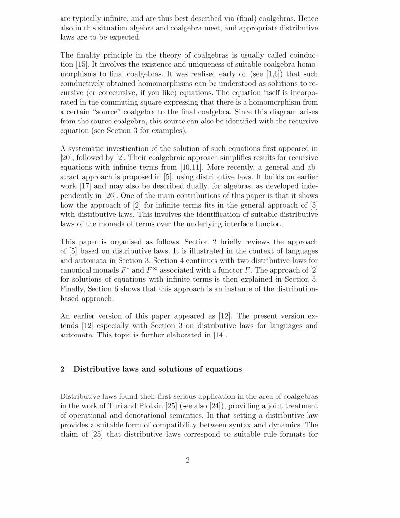
Definition 1 Let (T, η, µ) be a monad on a category C, and F : C → C be anarbitrary functor. A distributive law of T over F is a natural transformation

TF +3λFT

making for each X ∈ C the following two diagrams commute.

FX

ηFX��

F (ηX)

))SSSSSSSSSSSSSSSS T 2FX

µFX��

T (λX)// TFTXλTX // FT 2X

F (µX)��

TFXλX

// FTX TFXλX

// FTX

Sometimes we shall consider the situation when F is a monad too. Whenλ then also preserves the unit and multiplication associated with F—in theobvious way, like above—we shall say that λ is a distributive law of monads.

The underlying idea is that the monad T describes the terms in some syn-tax, and that the functor F is the interface for transitions on a state space.Intuitively, the presence of the distributive law tells us that the terms and be-haviours interact appropriately. The associated notion of model is a so-calledλ-bialgebra.

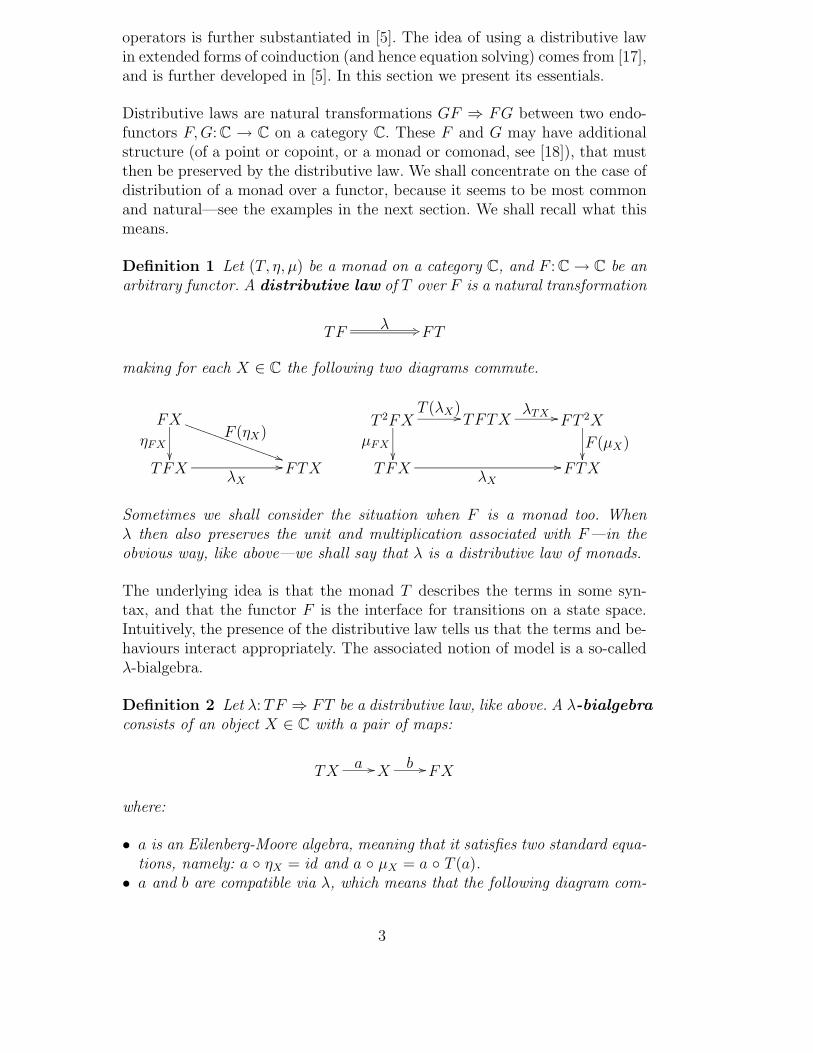
Definition 2 Let λ: TF ⇒ FT be a distributive law, like above. A λ-bialgebraconsists of an object X ∈ C with a pair of maps:

TXa // X

b // FX

where:

• a is an Eilenberg-Moore algebra, meaning that it satisfies two standard equa-tions, namely: a ◦ ηX = id and a ◦ µX = a ◦ T (a).

• a and b are compatible via λ, which means that the following diagram com-

3

mutes.

TX

T (b)��

a // Xb // FX

TFXλX

// FTX

F (a)OO

A map of λ-bialgebras, from (TXa

−→ Xb

−→ FX) to (TYc

−→ Yd

−→ FY )is a map f : X → Y in C that is both a map of algebras and of coalgebras:f ◦ a = c ◦ T (f) and d ◦ f = F (f) ◦ b.

The following result is standard.

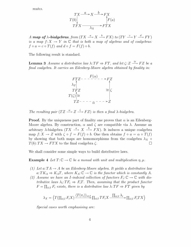
Lemma 3 Assume a distributive law λ: TF ⇒ FT , and let ζ: Z∼=−→ FZ be a

final coalgebra. It carries an Eilenberg-Moore algebra obtained by finality in:

FTZ //________F (α)

FZ

TFZ

λZ

OO

TZ

T (ζ) ∼=

OO

//_________α Z

∼= ζ

OO

The resulting pair (TZα

−→ Zζ

−→ FZ) is then a final λ-bialgebra.

Proof. By the uniqueness part of finality one proves that α is an Eilenberg-Moore algebra. By construction, α and ζ are compatible via λ. Assume an

arbitrary λ-bialgebra (TXa

−→ Xb

−→ FX). It induces a unique coalgebramap f : X → Z with ζ ◦ f = F (f) ◦ b. One then obtains f ◦ a = α ◦ T (f)by showing that both maps are homomorphisms from the coalgebra λX ◦T (b): TX → FTX to the final coalgebra ζ. �

We shall consider some simple ways to build distributive laws.

Example 4 Let T : C → C be a monad with unit and multiplication η, µ.

(1) Let a: TA → A be an Eilenberg-Moore algebra. It yields a distributive lawa: TKA ⇒ KAT , where KA: C → C is the functor which is constantly A.

(2) Assume we have an I-indexed collection of functors Fi: C → C with dis-tributive laws λi: TFi ⇒ FiT . Then, assuming that the product functorF =

∏

i∈I Fi exists, there is a distributive law λ: TF ⇒ FT given by

λX =(

T (∏

i∈I FiX)〈T (πi)〉i∈I //

∏

i∈I TFiX

∏

i∈I λi // ∏i∈I FiTX

)

Special cases worth emphasising are:

4

• I = {1, 2}, describing the distributive law T (F1 ×F2) ⇒ F1T ×F2T fora binary product from [5, Lemma 4.4.5];

• each Fi is equal to G, so that F is the exponent functor GI , with“strength” distributive law T (GI) ⇒ (GT )I .

(3) Dually, if T preserves coproducts, one can construct a distributive lawT (

∐

i∈I Fi) ⇒ (∐

i∈I Fi)T from laws TFi ⇒ FiT .(4) If our category C is Sets, and the functor T preserves weak pullbacks,

then there is a distributive law of monads TP ⇒ PT , where P is thepowerset monad. This construction comes from [13], and is called the“power law”. Here we sketch the essentials.

We associate the so-called “relation lifting” Rel(T ) with T . It is a func-tor that maps a relation 〈r1, r2〉: R � X × Y to a relation Rel(T )(R) �

T (X) × T (Y ) by taking the image of the map 〈T (r1), T (r2)〉: T (R) →T (X) × T (Y ). Applying this relation lifting to the inhabitation relation∈X� X×P(X) yields Rel(T )(∈X) � TX×TP(X). Then we can defineλX : TP(X) → P(TX) as:

λX(u) = {a ∈ TX | 〈a, u〉 ∈ Rel(T )(∈X)}.

In [13] it is shown that λ preserves the powerset monad structure. Butit also preserves the unit η and multiplication µ of the monad T in casethe natural transformations η, µ are Cartesian. This means that theirnaturality squares are pullbacks.

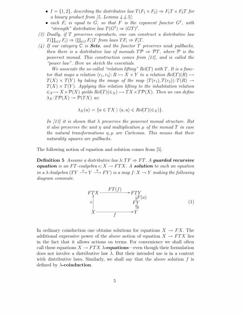
The following notion of equation and solution comes from [5].

Definition 5 Assume a distributive law λ: TF ⇒ FT . A guarded recursive

equation is an FT -coalgebra e: X → FTX. A solution to such an equation

in a λ-bialgebra (TYa

−→ Yb

−→ FY ) is a map f : X → Y making the followingdiagram commute.

FTXFT (f) // FTY

F (a)��FY

X

e

OO

f// Y

bOO (1)

In ordinary coinduction one obtains solutions for equations X → FX. Theadditional expressive power of the above notion of equation X → FTX liesin the fact that it allows actions on terms. For convenience we shall oftencall these equations X → FTX λ-equations—even though their formulationdoes not involve a distributive law λ. But their intended use is in a contextwith distributive laws. Similarly, we shall say that the above solution f isdefined by λ-coinduction.

5

This notion of solution may seem a bit strange at first, but becomes morenatural in light of the following result (see also [5, Lemma 4.3.4]).

Proposition 6 There exists a bijective correspondence between λ-equations

e: X → FTX and λ-bialgebras (T 2XµX−→ TX

d−→ FTX) with free algebra

µX .

Moreover, let (TYa

−→ Yb

−→ FY ) be a λ-bialgebra. Then there is a bijectivecorrespondence between solutions f : X → Y as in (1) and bialgebra mapsg: TX → Y —for the associated λ-equations and λ-bialgebras. �

Now we can formulate the main result of this distribution-based approach tosolving equations. It is the dual of [26, Theorem 1].

Theorem 7 Let F : C → C be a functor with a final coalgebra Z∼=−→ FZ. For

each monad T with distributive law λ: TF ⇒ FT there are unique solutionsto λ-equations in the final λ-bialgebra (TZ → Z → FZ) from Lemma 3.

Proof. For a λ-equation e: X → FTX, a solution in (TZ → Z → FZ) isby the previous proposition the same thing as a map of λ-bialgebras from theassociated (T 2X → TX → FTX) to (TZ → Z → FZ). Since the latter isfinal, there is precisely one such solution. �

In the next section, and also in Example 13, we present illustrations.

3 Kleene algebras and differential equations for languages

This section contains two applications of distributive laws in the context oflanguages: first, in order to obtain a “language” monad whose algebras areKleene algebras, and second, to describe differential equations for languageswith solutions as in the previous section.

3.1 Kleene algebras

A basic observation and starting point in this subsection is that there is a“power” distributive law π in:

P(X)? πX //P(X?)

〈u1, . . . , un〉� // {〈x1, . . . , xn〉 | ∀i ≤ n. xi ∈ ui}

(2)

6

It is obtained from the construction in Example 4 (4), using that the list monad(−)? is Cartesian. In order to investigate the consequence we use the followinggeneral result about distributive laws between monads. It is standard, andmay be traced back to [7,16,4] or [25].

Proposition 8 Let π: ST ⇒ TS be a distributive law between monads S andT on a category C. Then:

(1) TS is a monad, with unit and multiplication given as:

η =

S!)KKKKK

KKKKK ηT S

Id

6>uuuuuuuuuu

ηS

(II

III

IIII

I

ηT

TS

T

5=ssssssssss TηS

µ =

T 2S"*MMMMM

MMMMM µT S

TSTS +3TπST 2S2

3;pppppppppp

T 2µS

#+NNNNN

NNNNN

µT S

TS

TS2

4<qqqqqqqqqqTµS

Moreover, there are obvious maps of monads S ⇒ TS and T ⇒ TS givenby units.

(2) There is an induced lifting of T to Eilenberg-Moore algebras of S as in:

Alg(S)

��

T // Alg(S)

��C

T// C

given by

SX��

X

7−→

STXπ��

TSX��

TX

This yields a new monad T . It can be shown that there is a bijectivecorrespondence between such liftings and distributive laws.

(3) There is an isomorphism of categories of algebras:

Alg(TS)∼= //

��;;

;;

;;;

;;;

;Alg(T )

xxrrrrr

Alg(S)

||xxxxx

C�

When we apply this result to our power law π: (−)?P ⇒ P(−)? from (2) weobtain a new monad L = P(−)? which we shall call the language monad.This name is chosen because the sets L(X) = P(X?) contain languages L ⊆X∗ with words over the alphabet X.

According to Proposition 8 (1), the unit ηX : X → L(X) is given by

ηX(x) = {〈x〉}.

7

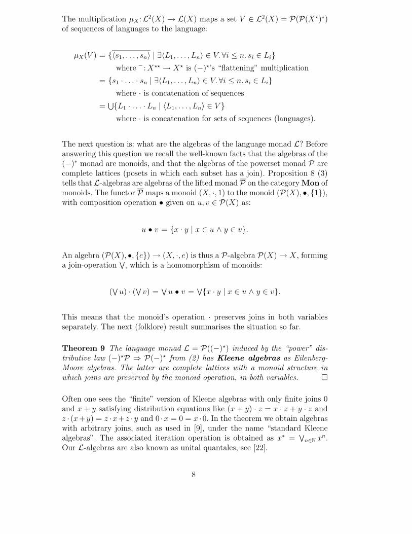
The multiplication µX :L2(X) → L(X) maps a set V ∈ L2(X) = P(P(X?)?)of sequences of languages to the language:

µX(V ) = {〈s1, . . . , sn〉 | ∃〈L1, . . . , Ln〉 ∈ V.∀i ≤ n. si ∈ Li}

where : X?? → X? is (−)?’s “flattening” multiplication

= {s1 · . . . · sn | ∃〈L1, . . . , Ln〉 ∈ V.∀i ≤ n. si ∈ Li}

where · is concatenation of sequences

=⋃{L1 · . . . · Ln | 〈L1, . . . , Ln〉 ∈ V }

where · is concatenation for sets of sequences (languages).

The next question is: what are the algebras of the language monad L? Beforeanswering this question we recall the well-known facts that the algebras of the(−)∗ monad are monoids, and that the algebras of the powerset monad P arecomplete lattices (posets in which each subset has a join). Proposition 8 (3)tells that L-algebras are algebras of the lifted monad P on the category Mon ofmonoids. The functor P maps a monoid (X, ·, 1) to the monoid (P(X), •, {1}),with composition operation • given on u, v ∈ P(X) as:

u • v = {x · y | x ∈ u ∧ y ∈ v}.

An algebra (P(X), •, {e}) → (X, ·, e) is thus a P-algebra P(X) → X, forminga join-operation

∨, which is a homomorphism of monoids:

(∨

u) · (∨

v) =∨

u • v =∨{x · y | x ∈ u ∧ y ∈ v}.

This means that the monoid’s operation · preserves joins in both variablesseparately. The next (folklore) result summarises the situation so far.

Theorem 9 The language monad L = P((−)?) induced by the “power” dis-tributive law (−)?P ⇒ P(−)? from (2) has Kleene algebras as Eilenberg-Moore algebras. The latter are complete lattices with a monoid structure inwhich joins are preserved by the monoid operation, in both variables. �

Often one sees the “finite” version of Kleene algebras with only finite joins 0and x + y satisfying distribution equations like (x + y) · z = x · z + y · z andz · (x+y) = z ·x+ z ·y and 0 ·x = 0 = x ·0. In the theorem we obtain algebraswith arbitrary joins, such as used in [9], under the name “standard Kleenealgebras”. The associated iteration operation is obtained as x∗ =

∨

n∈N xn.Our L-algebras are also known as unital quantales, see [22].

8

The set of languages L(X) carries a free Kleene algebra structure µX :L2(X) →L(X), with the familiar structure induced by the multiplication µ:

0 = µX(∅) = ∅

1 = µX({〈〉}) = {〈〉}

L1 · L2 = µX({〈L1, L2〉}) = {s1 · s2 | s1 ∈ L1 ∧ s2 ∈ L2}∨

i∈I Li = µX({〈Li〉 | i ∈ I}) =⋃

i∈I Li

L∗ = µX({〈L, . . . , L〉︸ ︷︷ ︸

n times

| n ∈ N}) =∨

n∈N Ln.

3.2 Differential equations for languages

In the previous subsection we have seen how sets of languages L(A) = P(A∗)form free Kleene algebras. Here we shall investigate them as (carriers of) finalcoalgebras. We shall do so in three stages, where the first one is well-known(and extensively studied in [23, Section 10]), and the second one comes from [5,Corollary 4.4.6]. The third one builds on the above language monad L.

3.2.1 Languages and deterministic automata

A deterministic automaton, with alphabet A, is a coalgebra 〈δ, ε〉: X → XA×2.The transition function δ maps a state together with an input to a new (next)state, and the output function ε tells of a state x ∈ X whether x is terminal(ε(x) = 1) or not (ε(x) = 0). We shall write D = (−)A × K2 for the functorinvolved. Typical for these deterministic automata is that for each state x andinput letter a ∈ A there is precisely one successor state x′ with x

a−→ x′,

i.e. with x′ = δ(x)(a).

As is well-known, the final D-coalgebra is given by the set of languages L(A) =P(A∗) over the alphabet A, with coalgebra structure 〈δ, ε〉:L(A) → L(A)A×2given by the “derivative” function and “is nullable” predicate (see [9,23]): forL ∈ L(A) and a ∈ A,

δ(L)(a) = La

= {σ ∈ A? | a · σ ∈ L}

ε(L) = (1 ⊆ L)

= (〈〉 ∈ L).

For an arbitrary D-coalgebra X → XA × 2, the induced homomorphism to

9

this final coalgebra,

XA × 2 //_________ L(A)A × 2

X

OO

//___________ L(A)

∼= 〈δ, ε〉OO

sends a state x ∈ X to the language accepted in this state, i.e. to the set ofthose strings 〈a1, . . . , an〉 ∈ A? leading from x to a terminal state.

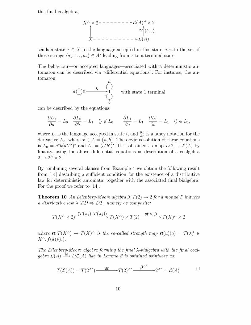
The behaviour—or accepted languages—associated with a deterministic au-tomaton can be described via “differential equations”. For instance, the au-tomaton:

0 b //a ;; 1

b

EE

a

��with state 1 terminal

can be described by the equations:

∂L0

∂a= L0

∂L0

∂b= L1 〈〉 6∈ L0

∂L1

∂a= L1

∂L1

∂b= L1 〈〉 ∈ L1,

where Li is the language accepted in state i, and ∂L∂x

is a fancy notation for thederivative Lx, where x ∈ A = {a, b}. The obvious solution of these equationsis L0 = a?b(a?b?)? and L1 = (a?b?)?. It is obtained as map L: 2 → L(A) byfinality, using the above differential equations as description of a coalgebra2 → 2A × 2.

By combining several clauses from Example 4 we obtain the following resultfrom [14] describing a sufficient condition for the existence of a distributivelaw for deterministic automata, together with the associated final bialgebra.For the proof we refer to [14].

Theorem 10 An Eilenberg-Moore algebra β: T (2) → 2 for a monad T inducesa distributive law λ: TD ⇒ DT , namely as composite:

T (XA × 2)〈T (π1), T (π2)〉 // T (XA) × T (2)

st × β // T (X)A × 2

where st: T (XA) → T (X)A is the so-called strength map st(u)(a) = T (λf ∈XA. f(a))(u).

The Eilenberg-Moore algebra forming the final λ-bialgebra with the final coal-gebra L(A)

∼=−→ DL(A) like in Lemma 3 is obtained pointwise as:

T (L(A)) = T (2A?

) st // T (2)A? βA?

// 2A?

= L(A). �

10

3.2.2 Languages and non-deterministic automata

A non-deterministic automaton, with alphabet A, is a coalgebra of the form〈δ, ε〉: X → P(X)A × 2. The transition function δ now maps a state x and aninput a to a set δ(x)(a) ⊆ X of successor states.

As observed in [5], there is a distributive law PD ⇒ DP , where D = (−)A×K2

as defined in Subsection 3.2.1. It is an instance of Theorem 10, because theset 2 = {0, 1} = P(1) carries a (free) P-monad structure, which is of coursegiven by union

∨wrt. the standard order 0 ≤ 1. The resulting distributive

law, say λP , is given explicitly by:

P(XA × 2)λP

X //P(X)A × 2

U� // 〈λa ∈ A. {f(a) | ∃b. (f, b) ∈ U}, ∃f. (f, 1) ∈ U〉

It is not hard to see that the (final) λP-bialgebra induced as in Lemma 3 (andgiven in Theorem 10) involves the union operation

⋃:P(L(A)) → L(A) in:

DPL(A) //________D(

⋃)

DL(A) = L(A)A × 2

PDL(A)

λPL(A)

OO

PL(A)

〈δ∪, ε∪〉

44

P(〈δ, ε〉) ∼=

OO

//__________ ⋃ L(A)

∼= 〈δ, ε〉

OO

In fact, this says that the union⋃

of languages can be defined by coinductionvia the D-coalgebra 〈δ∪, ε∪〉 given by:

ε∪(U) = (〈〉 ∈⋃

U) and δ∪(U)(a) = {La | L ∈ U}.

One of the nice observations in [5], see its Corollary 4.4.6, is that thelanguages associated with a non-deterministic automaton can be defined byλP-coinduction, i.e. as solution of a λP-equation, namely of the automatonX → DP(X) = P(X)A × 2 itself, like in:

P(X)A × 2 = DP(X) //________ DPL(A)

D(⋃

)��

DL(A) = L(A)A × 2

X

OO

//__________ L(A)

∼=OO

11

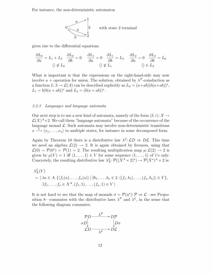
For instance, the non-deterministic automaton

1

b��

0

a55kkkkkkkkkkkk

a))SSSSSSSSSSSS

2b

^^ with state 2 terminal

gives rise to the differential equations

∂L0

∂a= L1 + L2

∂L0

∂b= 0

〈〉 6∈ L0

∂L1

∂a= 0

∂L1

∂b= L2

〈〉 6∈ L1

∂L2

∂a= 0

∂L2

∂b= L0

〈〉 ∈ L2

What is important is that the expressions on the right-hand-side may nowinvolve a + operation for union. The solution, obtained by λP-coinduction asa function L: 3 → L(A) can be described explicitly as L0 = (a+ab)(b(a+ab))?,L1 = b(b(a + ab))? and L2 = (b(a + ab))?.

3.2.3 Languages and language automata

Our next step is to use a new kind of automata, namely of the form 〈δ, ε〉: X →L(X)A×2. We call them “language automata” because of the occurrence of thelanguage monad L. Such automata may involve non-deterministic transitionsx

a−→ 〈x1, . . . , xn〉 to multiple states, for instance in some decomposed form.

Again by Theorem 10 there is a distributive law λL:LD ⇒ DL. This timewe need an algebra L(2) → 2. It is again obtained by freeness, using thatL(0) = P(0?) = P(1) = 2. The resulting multiplication map µ:L(2) → 2 isgiven by µ(V ) = 1 iff 〈1, . . . , 1〉 ∈ V for some sequence 〈1, . . . , 1〉 of 1’s only.Concretely, the resulting distributive law λL

X :P((XA × 2)?) → P(X?)A × 2 is:

λLX(V )

= 〈λa ∈ A. {〈f1(a), . . . , fn(a)〉 | ∃b1, . . . , bn ∈ 2. 〈(f1, b1), . . . , (fn, bn)〉 ∈ V },

∃f1, . . . , fn ∈ XA. (f1, 1), . . . , (fn, 1) ∈ V 〉

It is not hard to see that the map of monads σ = P(η?):P ⇒ L—see Propo-sition 8—commutes with the distributive laws λP and λL, in the sense thatthe following diagram commutes.

PD

σD��

λP// DP

Dσ��

LDλL

// DL

12

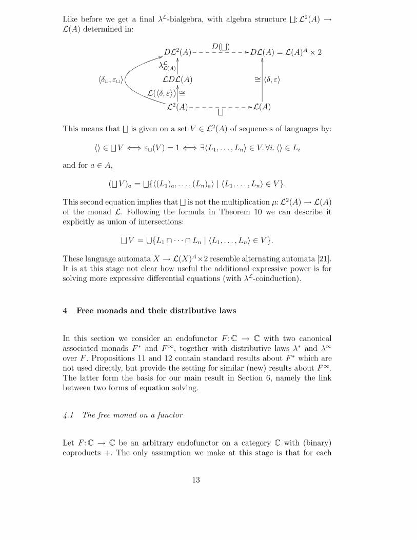
Like before we get a final λL-bialgebra, with algebra structure⊔

:L2(A) →L(A) determined in:

DL2(A) //_________D(

⊔)

DL(A) = L(A)A × 2

LDL(A)

λLL(A)

OO

L2(A)

〈δt, εt〉

44

L(〈δ, ε〉) ∼=

OO

//__________ ⊔ L(A)

∼= 〈δ, ε〉

OO

This means that⊔

is given on a set V ∈ L2(A) of sequences of languages by:

〈〉 ∈⊔

V ⇐⇒ εt(V ) = 1 ⇐⇒ ∃〈L1, . . . , Ln〉 ∈ V.∀i. 〈〉 ∈ Li

and for a ∈ A,

(⊔

V )a =⊔{〈(L1)a, . . . , (Ln)a〉 | 〈L1, . . . , Ln〉 ∈ V }.

This second equation implies that⊔

is not the multiplication µ:L2(A) → L(A)of the monad L. Following the formula in Theorem 10 we can describe itexplicitly as union of intersections:

⊔V =

⋃{L1 ∩ · · · ∩ Ln | 〈L1, . . . , Ln〉 ∈ V }.

These language automata X → L(X)A×2 resemble alternating automata [21].It is at this stage not clear how useful the additional expressive power is forsolving more expressive differential equations (with λL-coinduction).

4 Free monads and their distributive laws

In this section we consider an endofunctor F : C → C with two canonicalassociated monads F ∗ and F∞, together with distributive laws λ∗ and λ∞

over F . Propositions 11 and 12 contain standard results about F ∗ which arenot used directly, but provide the setting for similar (new) results about F ∞.The latter form the basis for our main result in Section 6, namely the linkbetween two forms of equation solving.

4.1 The free monad on a functor

Let F : C → C be an arbitrary endofunctor on a category C with (binary)coproducts +. The only assumption we make at this stage is that for each

13

object X ∈ C the functor X + F (−): C → C has an initial algebra. We shalluse the following notation. The carrier of this initial algebra will be writtenas F ∗(X) with structure map given as:

X + F (F ∗(X))αX∼=

// F ∗(X)

Further, we shall write

ηX = αX ◦ κ1 τX = αX ◦ κ2,

so that αX = [ηX , τX ].

The mapping X 7→ F ∗(X) is functorial: for f : X → Y we get:

X + F (F ∗(X))

αX ∼=��

//_________id + F (F ∗(f))

X + F (F ∗(Y ))

[ηY ◦ f, τY ]��

F ∗(X) //_____________

F ∗(f)F ∗(Y )

This means that

F ∗(f) ◦ ηX = ηY ◦ f F ∗(f) ◦ τX = τY ◦ F (F ∗(f)),

i.e. that η: id ⇒ F ∗ and τ : FF ∗ ⇒ F ∗ are natural transformations.

Next we establish that F ∗ is a monad. The multiplication µ is obtained in:

F ∗(X) + F (F ∗(F ∗(X)))

αF ∗(X) ∼=��

//_________id + F (µX)

F ∗(X) + F (F ∗(X))

[id, τX ]��

F ∗(F ∗(X)) //_______________µX

F ∗(X)

This yields one of the monad equations, namely µX ◦ ηF ∗(X) = id. The relatedequation µX ◦ F ∗(ηX) = id follows from uniqueness of algebra maps αX →αX :

µX ◦ F ∗(ηX) ◦ αX = µX ◦ [ηF ∗(X) ◦ ηX , τF ∗(X)] ◦ (id + F (F ∗(ηX)))

= [ηX , τX ◦ F (µX)] ◦ (id + F (F ∗(ηX)))

= αX ◦ (id + F (µX ◦ F ∗(ηX))).

Similarly, the other requirements making F ∗ a monad are obtained.

The following standard result sums up the situation.

Proposition 11 Let F : C → C with induced monad (F ∗, η, µ) be as describedabove.

14

(1) The mapping X 7→ [F (F ∗(X))τX−→ F ∗(X)] forms a left adjoint to the

forgetful functor U :Alg(F ) → C. The monad induced by this adjunctionis (F ∗, η, µ).

(2) The mapping σX = τX ◦ F (ηX): F (X) → F ∗(X) yields a natural trans-formation F ⇒ F ∗ that makes F ∗ the free monad on F . �

The next observation shows that the monad F ∗ of (finite) F -terms fits withthe behaviour of F . It follows from a general observation (made for instancein [5]) that distributive laws F ∗G ⇒ GF ∗ correspond to ordinary naturaltransformations FG ⇒ GF ∗. Hence by taking G = F and unit FF ⇒ FF ∗

one gets F ∗F ⇒ FF ∗. But here we shall present the construction explicitly.

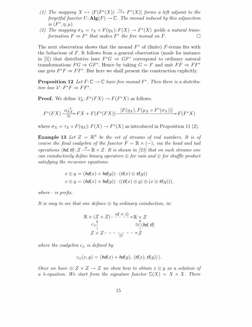
Proposition 12 Let F : C → C have free monad F ∗. Then there is a distribu-tive law λ∗: F ∗F ⇒ FF ∗.

Proof. We define λ∗X : F ∗(FX) → F (F ∗X) as follows.

F ∗(FX)α−1

FX∼=

// FX + F (F ∗(FX))[F (ηX), F (µX ◦ F ∗(σX))] // F (F ∗X)

where σX = τX ◦ F (ηX): F (X) → F ∗(X) as introduced in Proposition 11 (2).

Example 13 Let Z = RN be the set of streams of real numbers. It is of

course the final coalgebra of the functor F = R × (−), via the head and tail

operations 〈hd, tl〉: Z∼=−→ R × Z. It is shown in [23] that on such streams one

can coinductively define binary operators ⊕ for sum and ⊗ for shuffle productsatisfying the recursive equations:

x ⊕ y = (hd(x) + hd(y)) · (tl(x) ⊕ tl(y))

x ⊗ y = (hd(x) × hd(y)) · ((tl(x) ⊗ y) ⊕ (x ⊗ tl(y))),

where · is prefix.

It is easy to see that one defines ⊕ by ordinary coinduction, in:

R × (Z × Z) //______id ×⊕

R × Z

Z × Z

c⊕OO

//________⊕ Z

∼= 〈hd, tl〉

OO

where the coalgebra c⊕ is defined by:

c⊕(x, y) = 〈hd(x) + hd(y), 〈tl(x), tl(y)〉 〉.

Once we have ⊕: Z × Z → Z we show how to obtain x ⊗ y as a solution ofa λ-equation. We start from the signature functor Σ(X) = X × X. There

15

is an obvious natural transformation ΣF ⇒ FΣ∗ given by (〈r, x〉, 〈s, y〉) 7−→〈r+s, (x, y)〉. By [5, Lemma 3.4.24] it lifts to a distributive law λ: Σ∗F ⇒ FΣ∗

involving the associated free monad Σ∗. The algebra ⊕: Σ(Z) → Z yields anEilenberg-Moore algebra [[− ]]: Σ∗(Z) → Z, which is by the same result of [5]a λ-bialgebra. Now we obtain ⊗ as solution in:

R × Σ∗(Z × Z) //_________id × Σ∗(⊗)

R × Σ∗(Z)

id × [[− ]]��

R × Z

Z × Z

d⊗

OO

//_____________⊗ Z

∼= 〈hd, tl〉OO

in which the λ-equation d⊗ is defined by:

d⊗(x, y) = 〈hd(x) × hd(y), (tl(x), y)⊕(x, tl(y))〉,

where ⊕ is a symbol for sum in the language of terms on pairs from Z × Z.Here we exploit the expressive power of the λ-approach, because we can nowwrite terms as second component.

Clearly, the above diagram says:

hd(x ⊗ y) = hd(x) × hd(y).

And also, as required:

tl(x ⊗ y) = ([[− ]] ◦ Σ∗(⊗) ◦ π2 ◦ d⊗)(x, y)

= ([[− ]] ◦ Σ∗(⊗))( (tl(x), y)⊕(x, tl(y)) )

= [[ (tl(x) ⊗ y)⊕(x ⊗ tl(y)) ]]

= (tl(x) ⊗ y) ⊕ (x ⊗ tl(y)).

4.2 The free iterative monad on a functor

Let, like in the previous section, F : C → C be an arbitrary endofunctor on acategory C with (binary) coproducts +. The assumption we now make is thatfor each object X ∈ C the functor X + F (−): C → C has a final coalgebra—instead of an initial algebra. We shall use the following notation. The carrierof this final calgebra will be written as F∞(X) with structure map given as:

F∞(X)ζX∼=

// X + F (F∞(X))

16

The sets F ∗(X) in the previous section are understood as the set of finiteterms of type F with free variables from X. Here we understand F∞(X) asthe set of both finite and infinite terms (or trees) with free variables in X.

Like before, we shall write:

ηX = ζ−1X ◦ κ1 τX = ζ−1

X ◦ κ2.

Functoriality of F∞ is obtained as follows. For f : X → Y in C we get:

Y + F (F∞(X)) //________id + F (F∞(f))

Y + F (F∞(Y ))

F∞(X)

(f + id) ◦ ζX

OO

//_____________

F∞(f)F∞(Y )

ζY∼=

OO

This means that

F∞(f) ◦ ηX = ηY ◦ f F∞(f) ◦ τX = τY ◦ F (F∞(f)),

i.e. that η: id ⇒ F∞ and τ : FF∞ ⇒ F∞ are natural transformations.

It is shown in [3,19] that F∞ is a monad 1 . The multiplication operationµ is rather complicated, and can best be introduced via substitution t[s/x].What we mean is replacing all occurrences (if any) of the variable x in theterm t by the term s, but now for possibly infinite terms. In most gen-eral form, this substitution t[−→s /−→x ] replaces all occurrences of all variablesx ∈ X simultaneously. In this way, substitution may be described as an oper-ation which tells how an X-indexed collection (sx)x∈X of terms sx ∈ F∞(Y )acts on a term t ∈ F∞(X). More precisely, substitution becomes an oper-ation subst(s): F∞(X) → F∞(Y ), for a function s: X → F∞(Y ). As usual,such a substitution operation should respect the term structure—i.e. be ahomomorphism—and be trivial on variables. Standardly, substitution is de-fined by induction on the structure of (finite) terms. But since we are dealinghere with possibly infinite terms, we have to use coinduction. This makes thesubstitution more challenging. In general, it is done as follows.

Lemma 14 Let X,Y be arbitrary sets. Each function s: X → F∞(Y ) givesrise to a coalgebraic substitution operator subst(s): F∞(X) → F∞(Y ),

1 Similar results appeared earlier in [20], but for the functor Y 7→ F (X + Y ).

17

namely the unique homomorphism of F -algebras:

F (F∞(X))

τX

��

F (subst(s))// F (F∞(Y ))

τY

��

X

ηX

��

s

&&MMMMMMMMMMMMMMMMM

with

F∞(X)subst(s)

// F∞(Y ) F∞(X)subst(s)

// F∞(Y )

Proof. We begin by defining a coalgebra structure on the coproduct F∞(Y )+F∞(X) of terms, namely as the vertical composite on the left below. This coal-gebra on F∞(Y ) + F∞(X) simply unravels on F∞(Y ) on the left componentof +, and it applies s to the variables in the right component.

Y + F (F∞(Y ) + F∞(X)) //_________idY + F (f)

Y + F (F∞(Y ))

F∞(Y ) + F (F∞(X))

[(idY + F (κ1)) ◦ ζY , κ2 ◦ F (κ2)]

OO

F∞(Y ) + (X + F (F∞(X)))

[κ1, s + id]

OO

F∞(Y ) + F∞(X)

idY + ζX

OO

//_____________

fF∞(Y )

∼= ζY

OO

One first proves that f ◦ κ1 is the identity, using uniqueness of coalgebra mapsζY → ζY . Then, f ◦ κ2 is the required map subst(s). �

In the remainder of this paper we shall make frequent use of this substitutionoperator subst(−). Computations with substitution are made much easier withthe following elementary results. Proofs are obtained via the uniqueness prop-erty of substitution.

Lemma 15 For s: X → F∞(Y ) we have:

(1) subst(ηX) = idF (X).(2) subst(s) ◦ F∞(f) = subst(s ◦ f), for f : Z → X.(3) subst(r) ◦ subst(s) = subst(subst(r) ◦ s), for r: Y → F∞(Z).(4) F∞(f) = subst(ηZ ◦ f), for f : Y → Z, and hence subst(F∞(f) ◦ s) =

F∞(f) ◦ subst(s).(5) subst(s) = [s, τY ◦ F (subst(s))] ◦ ζX . �

Proposition 16 The map µX = subst(idF∞(X)): F∞(F∞(X)) → F∞(X) makes

the triple (F∞, η, µ) a monad.

18

This monad F∞ is called the iterative monad on F , via the natural transfor-mation σ = τ ◦ Fη: F ⇒ F∞.

In [2] it is shown that F∞ is in fact a free iterative monad, in a suitable sense.This freeness is not relevant here.

Proof. We check the monad equations, using Lemma 15.

µX ◦ ηF∞X = subst(idF∞(X)) ◦ ηF∞X

= idF∞(X).

µX ◦ F∞(ηX) = subst(idF∞(X)) ◦ F∞(ηX)

= subst(idF∞(X) ◦ ηX)

= idF∞(X).

µX ◦ F∞(µX) = subst(idF∞(X)) ◦ F∞(µX)

= subst(µX)

= subst(subst(idF∞(X)) ◦ idF∞(F∞(X)))

= subst(idF∞(X)) ◦ subst(idF∞(F∞(X)))

= µX ◦ µF∞(X). �

The following is less standard.

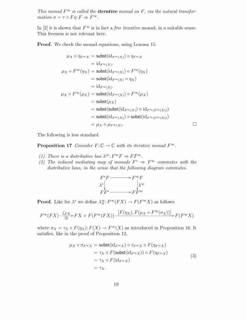
Proposition 17 Consider F : C → C with its iterative monad F∞.

(1) There is a distributive law λ∞: F∞F ⇒ FF∞.(2) The induced mediating map of monads F ∗ ⇒ F∞ commutes with the

distributive laws, in the sense that the following diagram commutes.

F ∗F

λ∗

��

// F∞F

λ∞

��FF ∗ // FF∞

Proof. Like for λ∗ we define λ∞X : F∞(FX) → F (F∞X) as follows:

F∞(FX)ζFX∼=

// FX + F (F∞(FX))[F (ηX), F (µX ◦ F∞(σX))] // F (F∞X)

where σX = τX ◦ F (ηX): F (X) → F∞(X) as introduced in Proposition 16. Itsatisfies, like in the proof of Proposition 12,

µX ◦ σF∞X = subst(idF∞X) ◦ τF∞X ◦ F (ηF∞X)

= τX ◦ F (subst(idF∞X)) ◦ F (ηF∞X)

= τX ◦ F (idF∞X)

= τX .

(3)

19

Then:

λ∞X ◦ ηFX = [F (ηX), F (µX ◦ F∞(σX))] ◦ ζFX ◦ ηFX

= [F (ηX), F (µX ◦ F∞(σX))] ◦ κ1

= F (ηX).

We shall use the following two auxiliary results:

µX ◦ σF∞X ◦ λ∞X = µX ◦ F∞(σX)

F (τX) ◦ F (λ∞X ) = λ∞

X ◦ τFX .(4)

We first prove the first equation, and use it immediately to prove the secondone.

µX ◦ σF∞X ◦ λ∞X

= [µX ◦ σF∞X ◦ F (ηX), µX ◦ σF∞X ◦ F (µX ◦ F∞(σX))] ◦ ζFX

by definition of λ

= [µX ◦ F∞(ηX) ◦ σX , µX ◦ F∞(µX ◦ F∞(σX)) ◦ σF∞FX ] ◦ ζFX

by naturality

= [µX ◦ ηF∞X ◦ σX , µX ◦ µF∞X ◦ F∞F∞(σX) ◦ σF∞FX ] ◦ ζFX

by the monad laws

= [µX ◦ F∞(σX) ◦ ηFX , µX ◦ F∞(σX) ◦ µFX ◦ σF∞FX ] ◦ ζFX

by naturality

= µX ◦ F∞(σX) ◦ [ηFX , τFX ] ◦ ζFX

by (3)

= µX ◦ F∞(σX)

by definition of η, τ .

F (τX) ◦ F (λ∞X )

= F (µX ◦ σF∞X ◦ λ∞X )

by (3)

= F (µX ◦ F∞(σX))

as we have just shown

= [F (ηX), F (µX ◦ F∞(σX))] ◦ κ2

obviously

= λ∞X ◦ τFX

by definition of τ.

20

Now we are ready to prove that λ∞ commutes with multiplications.

λ∞X ◦ µFX

= λ∞X ◦ [id, τFX ◦ F (µFX)] ◦ ζF∞FX by Lemma 15 (5)

= [λ∞X , λ∞

X ◦ τFX ◦ F (µFX)] ◦ ζF∞FX

(4)= [λ∞

X , F (τX ◦ λ∞X ◦ µFX)] ◦ ζF∞FX

(3)= [λ∞

X , F (µX ◦ σF∞X ◦ λ∞X ◦ µFX)] ◦ ζF∞FX

(4)= [λ∞

X , F (µX ◦ F∞(σX) ◦ µFX)] ◦ ζF∞FX

= [λ∞X , F (µX ◦ µF∞X ◦ F∞F∞(σX))] ◦ ζF∞FX

= [λ∞X , F (µX ◦ F∞(µX ◦ F∞(σX)))] ◦ ζF∞FX

(4)= [λ∞

X , F (µX ◦ F∞(µX ◦ σF∞X ◦ λ∞X ))] ◦ ζF∞FX

= [id, F (µX ◦ µF∞X ◦ F∞(σF∞X))] ◦ (λ∞X + F (F∞λ∞

X )) ◦ ζF∞FX

= F (µX) ◦ [F (ηF∞X), F (µF∞X ◦ F∞(σF∞X))] ◦ ζFF∞X ◦ F∞(λ∞X )

by definition of F∞ on morphisms

= F (µX) ◦ λ∞F∞X ◦ F∞(λ∞

X ).

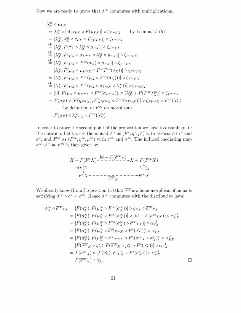
In order to prove the second point of the proposition we have to disambiguatethe notation. Let’s write the monad F ∗ as (F ∗, η∗, µ∗) with associated τ ∗ andσ∗, and F∞ as (F∞, η∞, µ∞) with τ∞ and σ∞. The induced mediating mapσ∞: F ∗ ⇒ F∞ is then given by:

X + F (F ∗X)

αX ∼=��

//_________id + F (σ∞

X)X + F (F∞X)

F ∗X //_____________

σ∞X

F∞X

ζX∼=

OO

We already know (from Proposition 11) that σ∞ is a homomorphism of monadssatisfying σ∞ ◦ σ∗ = σ∞. Hence σ∞ commutes with the distributive laws:

λ∞X ◦ σ∞

FX = [F (η∞X ), F (µ∞

X ◦ F∞(σ∞X ))] ◦ ζFX ◦ σ∞

FX

= [F (η∞X ), F (µ∞

X ◦ F∞(σ∞X ))] ◦ (id + F (σ∞

FX)) ◦ α−1FX

= [F (η∞X ), F (µ∞

X ◦ F∞(σ∞X ) ◦ σ∞

FX)] ◦ α−1FX

= [F (η∞X ), F (µ∞

X ◦ σ∞F∞X ◦ F ∗(σ∞

X ))] ◦ α−1FX

= [F (η∞X ), F (µ∞

X ◦ σ∞F∞X ◦ F ∗(σ∞

X ◦ σ∗X))] ◦ α−1

FX

= [F (σ∞X ◦ η∗

X), F (σ∞X ◦ µ∗

X ◦ F ∗(σ∗X))] ◦ α−1

FX

= F (σ∞X) ◦ [F (η∗

X), F (µ∗X ◦ F ∗(σ∗

X))] ◦ α−1FX

= F (σ∞X) ◦ λ∗

X . �

21

5 Iteration and solutions of equations

The material in this section comes (again) from [2]. In Definition 5 we haveseen an abstract notion of λ-equation and solution. A bit more concretely,for a functor F , a set of recursive equations—often simply called a recursiveequation—consists first of all of a set X of recursive variables. For each variablex ∈ X we have a corresponding term t in an equation x = t. We shall allowthis term to be infinite. The term t may involve both variables from an alreadygiven set Y , and from our new set of recursive variables X. Hence t ∈ F∞(Y +X). Summarising, a recursive equation is a map e: X → F∞(Y + X).We shall often call such an e a ∞-equation, in contrast to a λ-equationX → FTX—as in Definition 5.

Definition 18 Let F : C → C be a functor, with for X ∈ C a final coalgebraF∞(X)

∼=−→ X + F (F∞(X)).

A solution for an ∞-equation e: X → F∞(Y + X) is a map sol(e): X →F∞(Y ) that produces an appropriate term sol(e)(x) for each recursive variablex ∈ X. This means that substituting the cotuple [ηY , sol(e)]: Y + X → F∞(Y )in e yields the solution sol(e), i.e.

sol(e)

= subst([ηY , sol(e)]) ◦ ein

Xe //

sol(e) ((QQQQQQQQQQQQQQQ F∞(Y + X)

subst([ηY , sol(e)])��

F∞(Y )

This shows that the solution is a fixed point of subst([ηY ,−]) ◦ e.

Like for λ-equations, we are interested in unique solutions for ∞-equations.Do they always exist? Not in trivial equations, like x = x, where any term is asolution. Such equations are standardly excluded by requiring that the termsof the recursive equation are ‘guarded’, i.e. that its terms are not variablesfrom X. This notion can also be formulated in a general categorical setting: an∞-equation e: X → F∞(Y +X) is called guarded if it factors (in a necessarilyunique way, assuming that coprojections κi are monos) as:

Y + F (F∞(Y + X))

κ1 + id��

(Y + X) + F (F∞(Y + X))

∼= ζ−1Y +X

��X e

//

g33

~{

yw

us

qo

ml

j i

F∞(Y + X)

(5)

22

This says that if we decompose the terms of e using the final coalgebra map,then we do not get variables from X.

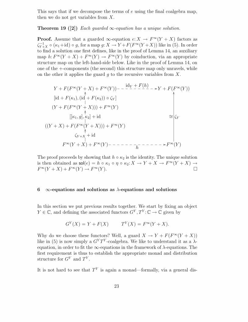
Theorem 19 ([2]) Each guarded ∞-equation has a unique solution.

Proof. Assume that a guarded ∞-equation e: X → F∞(Y + X) factors asζ−1Y +X ◦ (κ1+id) ◦ g, for a map g: X → Y +F (F∞(Y +X)) like in (5). In order

to find a solution one first defines, like in the proof of Lemma 14, an auxiliarymap h: F∞(Y + X) + F∞(Y ) → F∞(Y ) by coinduction, via an appropriatestructure map on the left-hand-side below. Like in the proof of Lemma 14, onone of the +-components (the second) this structure map only unravels, whileon the other it applies the guard g to the recursive variables from X.

Y + F (F∞(Y + X) + F∞(Y )) //__________idY + F (h)

Y + F (F∞(Y ))

(Y + F (F∞(Y + X))) + F∞(Y )

[id + F (κ1), (id + F (κ2)) ◦ ζY ]

OO

((Y + X) + F (F∞(Y + X))) + F∞(Y )

[[κ1, g], κ2] + id

OO

F∞(Y + X) + F∞(Y )

ζY +X + id

OO

//______________

hF∞(Y )

∼= ζY

OO

The proof proceeds by showing that h ◦ κ2 is the identity. The unique solutionis then obtained as sol(e) = h ◦ κ1 ◦ η ◦ κ2: X → Y + X → F∞(Y + X) →F∞(Y + X) + F∞(Y ) → F∞(Y ). �

6 ∞-equations and solutions as λ-equations and solutions

In this section we put previous results together. We start by fixing an objectY ∈ C, and defining the associated functors GY , T Y : C → C given by

GY (X) = Y + F (X) T Y (X) = F∞(Y + X).

Why do we choose these functors? Well, a guard X → Y + F (F∞(Y + X))like in (5) is now simply a GY T Y -coalgebra. We like to understand it as a λ-equation, in order to fit the ∞-equations in the framework of λ-equations. Thefirst requirement is thus to establish the appropriate monad and distributionstructure for GY and T Y .

It is not hard to see that T Y is again a monad—formally, via a general dis-

23

tributive law monads—with unit and multiplication:

ηYX = η∞

Y +X ◦ κ2 : X −→ Y + X −→ F∞(Y + X)

µYX = subst([η∞

Y +X ◦ κ1, id]) : F∞(Y + F∞(Y + X)) −→ F∞(Y + X).

For convenience we shall drop the superscript Y whenever confusion is unlikely.

Next we note that T Y is isomorphic to (GY )∞, since each (GY )∞(X) formsby construction the final coalgebra for the mapping:

X + GY (−) = X + (Y + F (−)) ∼= (Y + X) + F (−).

Hence (GY )∞(X) ∼= F∞(Y + X) = T Y (X). Proposition 17 then yields therequired distributive law. The next lemma describes it concretely.

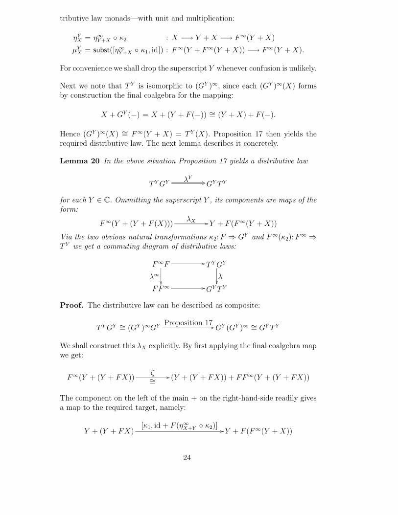
Lemma 20 In the above situation Proposition 17 yields a distributive law

T Y GY +3λY

GY T Y

for each Y ∈ C. Ommitting the superscript Y , its components are maps of theform:

F∞(Y + (Y + F (X)))λX // Y + F (F∞(Y + X))

Via the two obvious natural transformations κ2: F ⇒ GY and F∞(κ2): F∞ ⇒

T Y we get a commuting diagram of distributive laws:

F∞F

λ∞

��

// T Y GY

�

FF∞ // GY T Y

Proof. The distributive law can be described as composite:

T Y GY ∼= (GY )∞GY Proposition 17 // GY (GY )∞ ∼= GY T Y

We shall construct this λX explicitly. By first applying the final coalgebra mapwe get:

F∞(Y + (Y + FX))ζ∼=

// (Y + (Y + FX)) + FF∞(Y + (Y + FX))

The component on the left of the main + on the right-hand-side readily givesa map to the required target, namely:

Y + (Y + FX)[κ1, id + F (η∞

X+Y ◦ κ2)] // Y + F (F∞(Y + X))

24

For the component on the right we have to do more work. We are done ifwe can find a map F∞(Y + (Y + FX)) → F∞(Y + X). Such a map can beobtained via substitution from:

Y + (Y + FX)[η∞

Y +X ◦ κ1, [η∞Y +X ◦ κ1, σ

∞Y +X ◦ F (κ2)]] // F∞(Y + X)

Putting the decomposition via ζ and the two parts of a cotuple together, weobtain the following complicated expression for the resulting distributive lawF∞(Y + (Y + F (X))) → Y + F (F∞(Y + X)).

λX = [ [κ1, id + F (η∞X+Y ◦ κ2)],

κ2 ◦ F (subst([η∞Y +X ◦ κ1, [η

∞Y +X ◦ κ1, σ

∞Y +X ◦ F (κ2)]])) ] ◦ ζY +(Y +FX).

It is not hard to check that the distributive laws are preserved, as claimed atthe end of the lemma. �

Lemma 21 For each Y ∈ C, the object F∞(Y ) carries a final λY -bialgebrastructure:

T Y (F∞(Y ))ξY // F∞(Y )

ζY∼=

// GY (F∞(Y ))

F∞(Y + F∞(Y )) Y + F (F∞(Y ))

where ξY = subst([η∞Y , id]).

Proof. By Lemma 3 there is on F∞(Y ) a unique Eilenberg-Moore algebrastructure T Y (F∞(Y )) → F∞(Y ) forming a final λY -bialgebra. We establishthat it is of the form ξY = subst([η∞

Y , id]) by checking that this ξY satisfies the

25

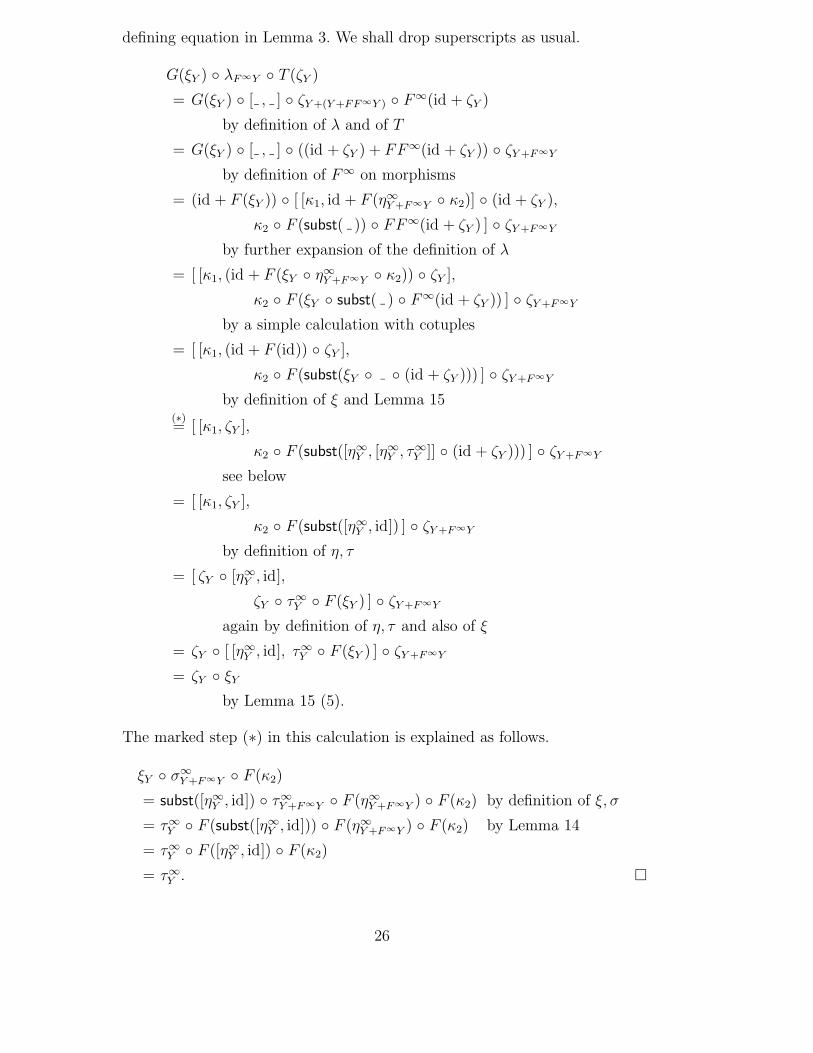
defining equation in Lemma 3. We shall drop superscripts as usual.

G(ξY ) ◦ λF∞Y ◦ T (ζY )

= G(ξY ) ◦ [ , ] ◦ ζY +(Y +FF∞Y ) ◦ F∞(id + ζY )

by definition of λ and of T

= G(ξY ) ◦ [ , ] ◦ ((id + ζY ) + FF∞(id + ζY )) ◦ ζY +F∞Y

by definition of F∞ on morphisms

= (id + F (ξY )) ◦ [ [κ1, id + F (η∞Y +F∞Y ◦ κ2)] ◦ (id + ζY ),

κ2 ◦ F (subst( )) ◦ FF∞(id + ζY ) ] ◦ ζY +F∞Y

by further expansion of the definition of λ

= [ [κ1, (id + F (ξY ◦ η∞Y +F∞Y ◦ κ2)) ◦ ζY ],

κ2 ◦ F (ξY ◦ subst( ) ◦ F∞(id + ζY )) ] ◦ ζY +F∞Y

by a simple calculation with cotuples

= [ [κ1, (id + F (id)) ◦ ζY ],

κ2 ◦ F (subst(ξY ◦ ◦ (id + ζY ))) ] ◦ ζY +F∞Y

by definition of ξ and Lemma 15(∗)= [ [κ1, ζY ],

κ2 ◦ F (subst([η∞Y , [η∞

Y , τ∞Y ]] ◦ (id + ζY ))) ] ◦ ζY +F∞Y

see below

= [ [κ1, ζY ],

κ2 ◦ F (subst([η∞Y , id]) ] ◦ ζY +F∞Y

by definition of η, τ

= [ ζY ◦ [η∞Y , id],

ζY ◦ τ∞Y ◦ F (ξY ) ] ◦ ζY +F∞Y

again by definition of η, τ and also of ξ

= ζY ◦ [ [η∞Y , id], τ∞

Y ◦ F (ξY ) ] ◦ ζY +F∞Y

= ζY ◦ ξY

by Lemma 15 (5).

The marked step (∗) in this calculation is explained as follows.

ξY ◦ σ∞Y +F∞Y ◦ F (κ2)

= subst([η∞Y , id]) ◦ τ∞

Y +F∞Y ◦ F (η∞Y +F∞Y ) ◦ F (κ2) by definition of ξ, σ

= τ∞Y ◦ F (subst([η∞

Y , id])) ◦ F (η∞Y +F∞Y ) ◦ F (κ2) by Lemma 14

= τ∞Y ◦ F ([η∞

Y , id]) ◦ F (κ2)

= τ∞Y . �

26

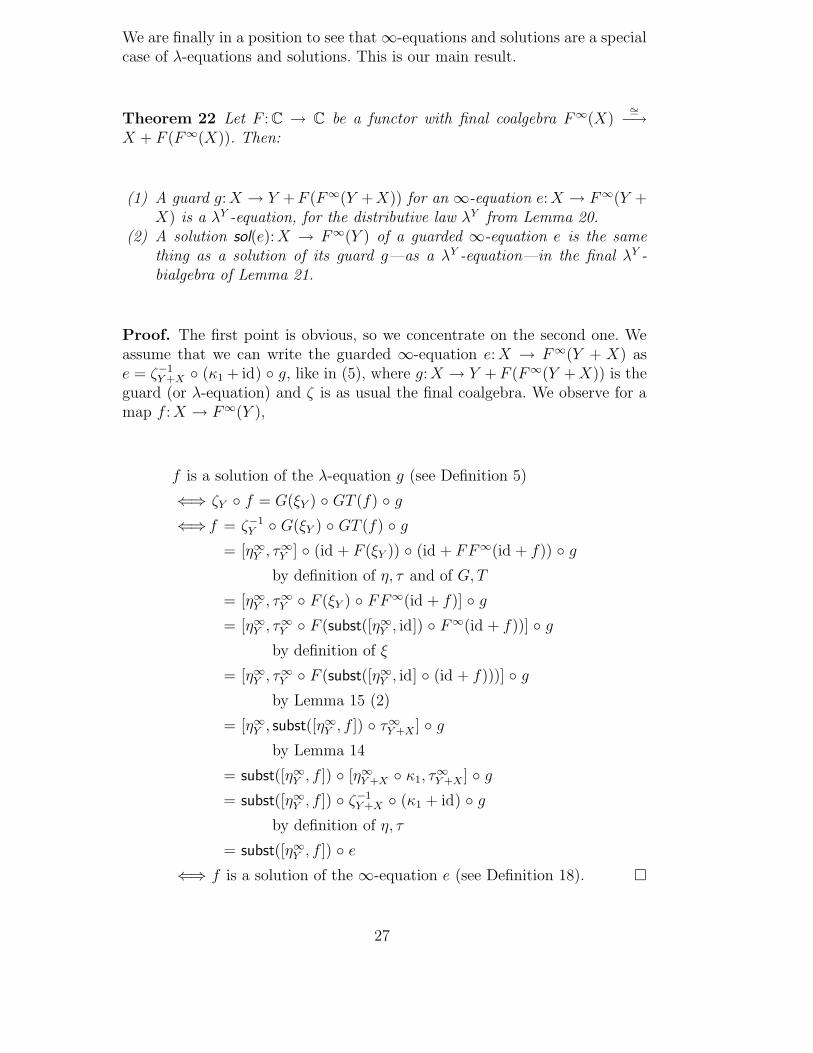
We are finally in a position to see that ∞-equations and solutions are a specialcase of λ-equations and solutions. This is our main result.

Theorem 22 Let F : C → C be a functor with final coalgebra F∞(X)∼=−→

X + F (F∞(X)). Then:

(1) A guard g: X → Y +F (F∞(Y +X)) for an ∞-equation e: X → F∞(Y +X) is a λY -equation, for the distributive law λY from Lemma 20.

(2) A solution sol(e): X → F∞(Y ) of a guarded ∞-equation e is the samething as a solution of its guard g—as a λY -equation—in the final λY -bialgebra of Lemma 21.

Proof. The first point is obvious, so we concentrate on the second one. Weassume that we can write the guarded ∞-equation e: X → F∞(Y + X) ase = ζ−1

Y +X ◦ (κ1 + id) ◦ g, like in (5), where g: X → Y + F (F∞(Y + X)) is theguard (or λ-equation) and ζ is as usual the final coalgebra. We observe for amap f : X → F∞(Y ),

f is a solution of the λ-equation g (see Definition 5)

⇐⇒ ζY ◦ f = G(ξY ) ◦ GT (f) ◦ g

⇐⇒ f = ζ−1Y ◦ G(ξY ) ◦ GT (f) ◦ g

= [η∞Y , τ∞

Y ] ◦ (id + F (ξY )) ◦ (id + FF∞(id + f)) ◦ g

by definition of η, τ and of G, T

= [η∞Y , τ∞

Y ◦ F (ξY ) ◦ FF∞(id + f)] ◦ g

= [η∞Y , τ∞

Y ◦ F (subst([η∞Y , id]) ◦ F∞(id + f))] ◦ g

by definition of ξ

= [η∞Y , τ∞

Y ◦ F (subst([η∞Y , id] ◦ (id + f)))] ◦ g

by Lemma 15 (2)

= [η∞Y , subst([η∞

Y , f ]) ◦ τ∞Y +X ] ◦ g

by Lemma 14

= subst([η∞Y , f ]) ◦ [η∞

Y +X ◦ κ1, τ∞Y +X ] ◦ g

= subst([η∞Y , f ]) ◦ ζ−1

Y +X ◦ (κ1 + id) ◦ g

by definition of η, τ

= subst([η∞Y , f ]) ◦ e

⇐⇒ f is a solution of the ∞-equation e (see Definition 18). �

27

7 Conclusion

We have illustrated the use of distributive laws in recursive equations (es-pecially for languages) and have unified the area by showing that one no-tion developed in [2] (following [20]) is an instance of a more general notionfrom [5,17,26] based on distributive laws.

Acknowledgments

Thanks to the anonymous referees, both of the current and of the earlierversion [12] of this paper, for suggesting many improvements, and also toIchiro Hasuo for his comments.

References

[1] P. Aczel. Non-well-founded sets. CSLI Lecture Notes 14, Stanford, 1988.

[2] P. Aczel, J. Adamek, S. Milius, and J. Velebil. Infinite trees and completelyiterative theories: a coalgebraic view. Theor. Comp. Sci., 300 (1-3):1–45, 2003.

[3] P. Aczel, J. Adamek, and J. Velebil. A coalgebraic view of infinite trees anditeration. In A. Corradini, M. Lenisa, and U. Montanari, editors, Coalgebraic

Methods in Computer Science, number 44 in Elect. Notes in Theor. Comp. Sci.Elsevier, Amsterdam, 2001.

[4] M. Barr and Ch. Wells. Toposes, Triples and Theories. Springer, Berlin, 1985.Revised and corrected version available from URL:www.cwru.edu/artsci/math/wells/pub/ttt.html.

[5] F. Bartels. On generalised coinduction and probabilistic specification formats.

Distributive laws in coalgebraic modelling. PhD thesis, Free Univ. Amsterdam,2004.

[6] J. Barwise and L.S. Moss. Vicious Circles: On the Mathematics of Non-

wellfounded Phenomena. CSLI Lecture Notes 60, Stanford, 1996.

[7] J. Beck. Distributive laws. In B. Eckman, editor, Seminar on Triples and

Categorical Homolgy Theory, number 80 in Lect. Notes Math., pages 119–140.Springer, Berlin, 1969.

[8] J.R.B. Cockett. Introduction to distributive categories. Math. Struct. in Comp.

Sci., 3:277–307, 1993.

[9] J.H. Conway. Regular Algebra and Finite Machines. Chapman and Hall, 1971.

28

[10] C.C. Elgot. Monadic computation and iterative algebraic theories. In H.E. Roseand J.C. Shepherson, editors, Logic Colloquium ’73, pages 175–230, Amsterdam,1975. North-Holland.

[11] C.C. Elgot, S.L. Bloom, and R. Tindell. The algebraic structure of rooted trees.Journ. Comp. Syst. Sci, 16:361–399, 1978.

[12] B. Jacobs. Relating two approaches to coinductive solution of recursiveequations. In J. Adamek and S. Milius, editors, Coalgebraic Methods in

Computer Science, number 106 in Elect. Notes in Theor. Comp. Sci. Elsevier,Amsterdam, 2004.

[13] B. Jacobs. Trace semantics for coalgebras. In J. Adamek and S. Milius, editors,Coalgebraic Methods in Computer Science, number 106 in Elect. Notes in Theor.Comp. Sci. Elsevier, Amsterdam, 2004.

[14] B. Jacobs. A bialgebraic review of regular expressions, deterministic automataand languages. Techn. Rep. ICIS-R05003, Inst. for Computing and InformationSciences, Radboud Univ. Nijmegen, 2005.

[15] B. Jacobs and J. Rutten. A tutorial on (co)algebras and (co)induction. EATCS

Bulletin, 62:222–259, 1997.

[16] P.T. Johnstone. Adjoint lifting theorems for categories of algebras. Bull. London

Math. Soc., 7:294–297, 1975.

[17] M. Lenisa. From set-theoretic coinduction to coalgebraic coinduction: someresults, some problems. In B. Jacobs and J. Rutten, editors, Coalgebraic

Methods in Computer Science, number 19 in Elect. Notes in Theor. Comp.Sci. Elsevier, Amsterdam, 1999.

[18] M. Lenisa, J. Power, and H. Watanabe. Distributivity for endofunctors, pointedand co-pointed endofunctors, monads and comonads. In H. Reichel, editor,Coalgebraic Methods in Computer Science, number 33 in Elect. Notes in Theor.Comp. Sci. Elsevier, Amsterdam, 2000.

[19] S. Milius. On iterable endofunctors. In R. Blute and P. Selinger, editors,Category Theory and Computer Science 2002, number 69 in Elect. Notes inTheor. Comp. Sci. Elsevier, Amsterdam, 2003.

[20] L.S. Moss. Parametric corecursion. Theor. Comp. Sci., 260(1-2):139–163, 2001.

[21] D.E. Muller and P.E. Schupp. Alternating automata on infinite trees. Theor.

Comp. Sci., 54(2/3):267–276, 1987.

[22] K.I. Rosenthal. Quantales and their applications. Number 234 in PitmanResearch Notes in Math. Longman Scientific & Technical, 1990.

[23] J. Rutten. Behavioural differential equations: a coinductive calculus of streams,automata, and power series. Theor. Comp. Sci., 308:1–53, 2003.

[24] D. Turi. Functorial operational semantics and its denotational dual. PhD thesis,Free Univ. Amsterdam, 1996.

29

[25] D. Turi and G. Plotkin. Towards a mathematical operational semantics. InLogic in Computer Science, pages 280–291. IEEE, Computer Science Press,1997.

[26] T. Uustalu, V. Vene, and A. Pardo. Recursion schemes from comonads. Nordic

Journ. Comput., 8(3):366–390, 2001.

30