Embed Size (px)
Citation preview
Portland State University Portland State University
PDXScholar PDXScholar
Civil and Environmental Engineering Undergraduate Honors Theses Civil and Environmental Engineering
Spring 2021
Distributionally Robust Optimization Utilizing Facility Distributionally Robust Optimization Utilizing Facility
Location Problems Location Problems
Elijah J. Kling Portland State University
Follow this and additional works at: https://pdxscholar.library.pdx.edu/cengin_honorstheses
Part of the Civil Engineering Commons, and the Transportation Engineering Commons
Let us know how access to this document benefits you.
Recommended Citation Recommended Citation Kling, Elijah J., "Distributionally Robust Optimization Utilizing Facility Location Problems" (2021). Civil and Environmental Engineering Undergraduate Honors Theses. 12. https://doi.org/10.15760/honors.1147
This Thesis is brought to you for free and open access. It has been accepted for inclusion in Civil and Environmental Engineering Undergraduate Honors Theses by an authorized administrator of PDXScholar. Please contact us if we can make this document more accessible: [email protected].
DISTRIBUTIONALLY ROBUST OPTIMIZATION UTILIZING
FACILITY LOCATION PROBLEMS
BY
Elijah Kling
A thesis submitted in partial fulfillment
of the requirement for the degree of
BACHELOR OF SCIENCE
IN
CIVIL AND ENVIRONMENTAL ENGINEERING
Thesis Advisor:
Dr. Avinash Unnikrishnan
Portland State University
©2021

ii
ACKNOWLEDGMENTS
I extend a huge thank you to Dr. Avinash Unnikrishnan, whose guidance and brilliance made this
work possible.
I would like to thank Darshan Chauhan, who provided the tools and examples which allowed for
this thesis to be completed.
I would also like to thank the National Science Foundation Grant number 1826337 “Collaborative
Research: Real-Time Stochastic Matching Models for Freight Electronic Marketplace” for
supporting this research.
Lastly, I would like to thank my instructors, professors, and peers for creating a unique and
motivating learning environment.
iii
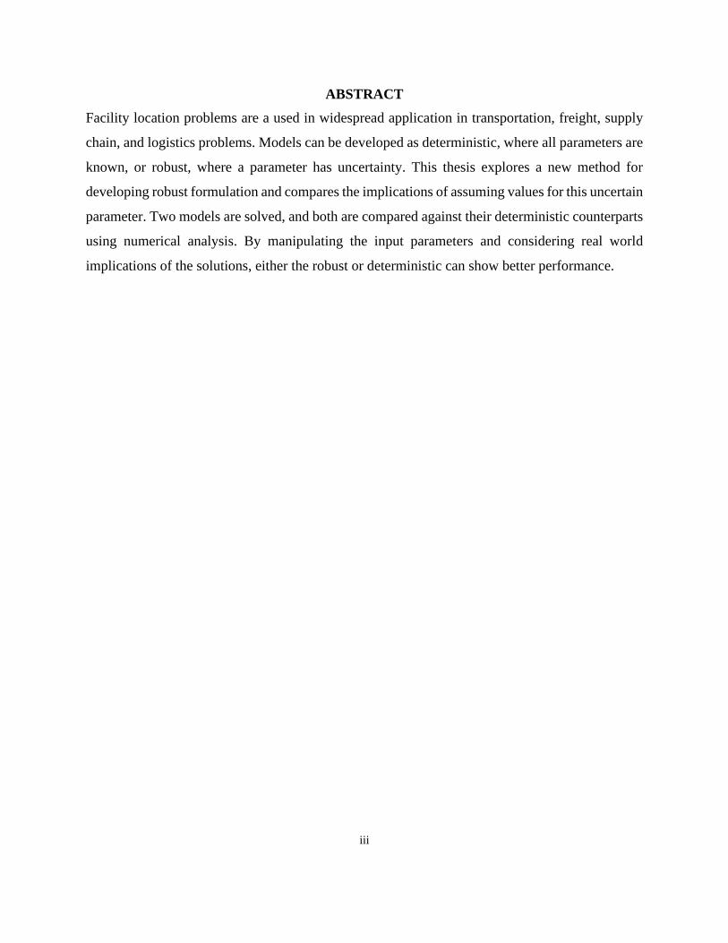
ABSTRACT
Facility location problems are a used in widespread application in transportation, freight, supply
chain, and logistics problems. Models can be developed as deterministic, where all parameters are
known, or robust, where a parameter has uncertainty. This thesis explores a new method for
developing robust formulation and compares the implications of assuming values for this uncertain
parameter. Two models are solved, and both are compared against their deterministic counterparts
using numerical analysis. By manipulating the input parameters and considering real world
implications of the solutions, either the robust or deterministic can show better performance.
iv
TABLE OF CONTENTS
1 INTRODUCTION ......................................................................................................................................... 1
2 PURPOSE ...................................................................................................................................................... 2
3 LITERATURE REVIEW ............................................................................................................................. 3
4 MODELS ....................................................................................................................................................... 4
4.1 MAXIMUM COVERAGE FLP ............................................................................................................................ 4 4.1.1 Nomenclature ......................................................................................................................................... 4 4.1.2 Deterministic Formulation .................................................................................................................... 5 4.1.3 Robust Formulation ............................................................................................................................... 5
4.2 MINIMUM COST FLP ...................................................................................................................................... 7 4.2.1 Nomenclature ......................................................................................................................................... 7 4.2.2 Deterministic Formulation .................................................................................................................... 8 4.2.3 Robust Formulation ............................................................................................................................... 8
5 NUMERICAL ANALYSIS AND RESULTS ............................................................................................ 11
5.1 MAXIMUM COVERAGE FLP .......................................................................................................................... 11 5.1.1 Effect of Varying Capacity ................................................................................................................... 12 5.1.2 Effect of Varying Coverage Radius ...................................................................................................... 13 5.1.3 Effect of Varying Facilities Located .................................................................................................... 14 5.1.4 Comparing Symmetric and Various Asymmetric Distributions ........................................................... 16 5.1.5 Maximum Coverage FLP Discussion .................................................................................................. 17
5.2 MINIMUM COST FLP .................................................................................................................................... 17 5.2.1 Model Solution Networks ..................................................................................................................... 20 5.2.2 MCS Results Considering Symmetric and Asymmetric Distributions .................................................. 21 5.2.3 Considering Penalty ............................................................................................................................ 21 5.2.4 Minimum Cost FLP Discussion ........................................................................................................... 22
5.3 EVALUATION OF 𝒅𝒊∗ ...................................................................................................................................... 23
6 CONCLUSION ............................................................................................................................................ 24
7 REFERENCES ............................................................................................................................................ 25
8 APPENDIX .................................................................................................................................................. 27
8.1 PYTHON CODE FOR MAXIMUM COVERAGE FLP ........................................................................................... 27 8.1.1 Deterministic........................................................................................................................................ 27 8.1.2 Robust .................................................................................................................................................. 29
8.2 PYTHON CODE FOR MINIMUM COST FLP ...................................................................................................... 31 8.2.1 Deterministic........................................................................................................................................ 31 8.2.2 Robust .................................................................................................................................................. 34
v
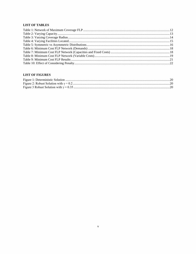
LIST OF TABLES
Table 1: Network of Maximum Coverage FLP ........................................................................................................... 12 Table 2: Varying Capacity ........................................................................................................................................... 13 Table 3: Varying Coverage Radius .............................................................................................................................. 14 Table 4: Varying Facilities Located............................................................................................................................. 15 Table 5: Symmetric vs Asymmetric Distributions ....................................................................................................... 16 Table 6: Minimum Cost FLP Network (Demands) ..................................................................................................... 18 Table 7: Minimum Cost FLP Network (Capacities and Fixed Costs) ......................................................................... 18 Table 8: Minimum Cost FLP Network (Variable Costs) ............................................................................................. 19 Table 9: Minimum Cost FLP Results .......................................................................................................................... 21 Table 10: Effect of Considering Penalty ...................................................................................................................... 22
LIST OF FIGURES
Figure 1: Deterministic Solution ................................................................................................................................. 20 Figure 2: Robust Solution with γ = 0.2 ........................................................................................................................ 20 Figure 3 Robust Solution with γ = 0.35 ....................................................................................................................... 20
1
1 INTRODUCTION
Transportation, supply chain, and freight systems are typically designed through maximizing
efficiency. This paper will primarily focus on facility location problems (FLP), which have
widespread application. Facility is used as a broad term including but not limited to factories,
seaports, schools, public transit stops, and more. A maximum coverage FLP is used in public sector
applications to locate facilities by maximizing the demand served. Examples of public sector
applications include locating post offices, health clinics, ambulances, fire departments, etc. FLPs
are also used in the private sector. Private sector applications will often use a cost minimization
perspective as maximizing coverage is not essential.
The FLPs which will be considered in this paper will include one public and one private sector
application. The problems are initially deterministic, meaning that no randomness is involved to
develop a solution. Each constraint which is accounted for in the problem is known, unchanging,
and not affected by chance. Using deterministic problems as a basis for development poses
concerns because many deterministic constraints are not a reality.
A robust problem will account for uncertainty. There are multiple ways to achieve this. For our
purposes, one parameter will be assumed to have a distribution with defined bounds. Using the
methods from (Ghosal and Wiesemann, 2020), an equivalent parameter will be generated to
encapsulate the uncertain parameter. The goal of this paper will be to create robust models which
are computationally quicker and easier to solve.

2
2 PURPOSE
An important theme in civil engineering problems is how much do we design for? That is, how
can we be certain that a design will meet the criteria without using too many resources, effort, and
labor? Designing to meet an average doesn’t work because failure occurs 50% of the time.
Designing something to never fail is incredibly costly and overengineered. Canon 1 of The
American Society of Civil Engineers (ASCE) Code of Ethics states that “Engineers shall hold
paramount the safety, health, and welfare of the public and shall strive to comply with the
principles of sustainable development in the performance of their professional duties.” (Code of
Ethics)
Above all else, a design should be safe and healthy to use. The most important criterion after that
is welfare of the public. The problem we are evaluating becomes clearer. When dealing with
uncertainty, we must be able to quantify what can be expected. From there we can ensure that
whatever we are designing for captures safety, health, and welfare of the public. When choosing
how to locate facilities, it is important to ensure that a decision maker can see how the uncertainty
is quantified. By creating a stochastic model, the certainty for which a constraint will be satisfied
can be controlled. For the purposes of this research, demand is considered as uncertain. Uncertain
demand will be implemented into two facility location models to show how well the stochastic
solution meets the objectives. To provide a reasonable design, the uncertain demand should be
permitted to exceed the capacity of the facility a very small fraction of the time. In both models
this is less than five percent of the time. A theme of this paper is to obtain a practical robust model
which provides better performance than its deterministic counterpart.
3
3 LITERATURE REVIEW
A plethora of work has been conducted on FLPs. (Church and ReVelle, 1974) outlines the
maximum coverage FLP which paved the road for the continuous development of problems in this
field. This literature review aims to illustrate the diversity of application though the following
relevant work. (Current et al., 2002) outlines the widespread application and usefulness of
maximum coverage FLPs. A model from (Esnaf and Küçükdeniz, 2009) shows a broader method
of locating facilities by eliminating the set of facilities to choose from. Instead, facilities are located
anywhere to maximize demand. (Arabani and Farahani, 2012) show the dynamics between
different minimum cost FLPs. (Chauhan et al., 2019) applies a maximum coverage FLP to drone-
delivery and demonstrates how FLPs will be adapted to changing infrastructure. (Karatas and
Dasci, 2020) shows how a FLP can incorporate more levels of facilities to maximize demand over
an entire supply chain system. (Arslan, 2021) develops a solution considering the choice to locate
a facility or route a vehicle. FLPs are incredibly diverse in their applications and continue to evolve
with development.
Many works also consider uncertainty. (Snyder, 2006) reviews FLP problems under uncertainty
and shows the diversity in objectives which have been developed. A study on linear optimization
problems by (Bertsimas and Sim, 2004) shows how robust solutions may be too conservative.
(Wang et al., 2002) shows algorithms considering M/M/1 queueing systems met with stochastic
demand. (Miranda and Garrido, 2004) utilize stochastic demand in their network design model
aimed at incorporating short- and medium-term decisions. (Baron et al., 2011) and (Gülpınar et
al., 2013) show various robust strategies for FLPs under uncertain demands. (Naoum-Sawaya and
Elhedhli, 2013) present a stochastic optimization model applied to ambulance deployment.
(Berglund and Kwon, 2014) present a robust FLP to minimize cost of hazardous waste
transportation. (Lutter et al., 2017) explore robust solutions to set covering problems through
studying mixed integer linear program problems. (Zhong et al., 2020) apply optimization to a
facility location and vehicle routing problem. (Chauhan et al., 2020) extends the work of (Chauhan
et al., 2019) and applies a robust optimization approach to an integer linear programming model.
(Basciftci et al., 2021) considers stochastic demands for a two-stage decision-dependent
optimization model. Considering uncertain parameters, particularly demand, is incredibly common
in FLPs and other network optimization models.
4
4 MODELS
The two models used to study the robust solution are a maximum coverage FLP and a minimum
cost FLP. The robust models will be developed using a method proposed by (Ghosal and
Wiesemann, 2020)
4.1 Maximum Coverage FLP
The objective of a maximum coverage FLP is in its name: to maximize the coverage. This type of
FLP is more applicable in the case of public sector development. The model presented is
capacitated and includes a coverage radius. For the purposes of maximizing infeasibility in
numerical analysis, the model will be assumed to have an infinite coverage radius.
4.1.1 Nomenclature
Sets
𝐼 Set of demand points
𝐽 Set of potential facility locations
Indices
𝑖 ∈ 𝐼
𝑗 ∈ 𝐽
Parameters
𝜀 Probability Parameter
𝛾 Deviation Parameter
𝑎𝑗 Importance of meeting demand point j
�̃�𝑖 Probabilistic demand of point 𝑖
𝑑𝑖 Nominal demand of point 𝑖
𝑈 Capacity
𝑠 Coverage radius
𝐿𝑖𝑗 Distance between demand point and facility location
𝑀𝑖𝑗 1 if 𝐿𝑖𝑗 ≤ 𝑠; ꝏ otherwise
𝑝 Maximum number of facilities to locate
Decision Variables
𝑥𝑗 Binary: Equal to 1 if facility 𝑖 is opened; 0 otherwise
5
𝑦𝑖𝑗 Binary: Equal to 1 if demand point 𝑖 is serving facility 𝑗; 0 otherwise
4.1.2 Deterministic Formulation
The objective is to maximize the coverage across all demand points (1).
𝑚𝑎𝑥𝑖𝑚𝑖𝑧𝑒 ∑ ∑ 𝑎𝑖𝑦𝑖𝑗𝑗∈𝐽𝑖∈𝐼 (1)
𝑆. 𝑇𝑜. ∑ 𝑀𝑖𝑗𝑑𝑖𝑦𝑖𝑗 ≤ 𝑈𝑥𝑗𝑖∈𝐼 , ∀ 𝑗 ∈ 𝐽 (2)
∑ 𝑀𝑖𝑗𝑦𝑖𝑗 ≤ 1,𝑗 ∈𝐽 ∀ 𝑖 ∈ 𝐼 (3)
𝑦𝑖𝑗 ≤ 𝑥𝑗 , ∀ 𝑖 ∈ 𝐼, 𝑗 ∈ 𝐽 (4)
∑ 𝑥𝑗 ≤ 𝑝𝑗∈𝐽 (5)
𝑥𝑗 ∈ {0, 1}, ∀ 𝑗 ∈ 𝐽 (6)
𝑦𝑖𝑗 ∈ {0, 1}, ∀ 𝑖 ∈ 𝐼, 𝑗 ∈ 𝐽 (7)
(2) ensures that demand does not exceed capacity. Constraint (3) prevents a single demand
point from mapping to more than one facility and (4) ensures that demand points are not
mapped to closed facilities. (5) controls how many facilities are opened and (6-7) are
variable definitions.
4.1.3 Robust Formulation
We begin with the deterministic problem. The nominal demand will now be considered as
uncertain. Letting �̃�𝑖 represent the uncertain demand, equation (8) is employed in place of (2) with
a confidence of at least 1 − 𝜀.
𝑚𝑎𝑥𝑖𝑚𝑖𝑧𝑒 ∑ ∑ 𝑎𝑖𝑦𝑖𝑗𝑀𝑖𝑗𝑗∈𝐽𝑖∈𝐼 (1)
𝑆. 𝑇𝑜. 𝑃(∑ 𝑀𝑖𝑗�̃�𝑖𝑦𝑖𝑗 ≤ 𝑈𝑥𝑗𝑖∈𝐼 ) ≥ 1 − 𝜀, ∀ 𝑗 ∈ 𝐽, 𝑃 ∈ ℙ (8)
∑ 𝑀𝑖𝑗𝑦𝑖𝑗 ≤ 1,𝑗 ∈𝐽 ∀ 𝑖 ∈ 𝐼 (3)
𝑦𝑖𝑗 ≤ 𝑥𝑗 , ∀ 𝑖 ∈ 𝐼, 𝑗 ∈ 𝐽 (4)
∑ 𝑥𝑗 ≤ 𝑝𝑗∈𝐽 (5)
6
𝑥𝑗 ∈ {0, 1}, ∀ 𝑗 ∈ 𝐽 (6)
𝑦𝑖𝑗 ∈ {0, 1}, ∀ 𝑖 ∈ 𝐼, 𝑗 ∈ 𝐽 (7)
Equation (8) can then be rewritten as
sup𝑃∈ℙ
𝑃 (∑ 𝑀𝑖𝑗�̃�𝑖𝑦𝑖𝑗 ≤ 𝑈𝑥𝑗𝑖∈𝐼 ) ≥ 1 − 𝜀, ∀ 𝑗 ∈ 𝐽 (9)
Let VAR1−𝜀,𝑃 be the 1 − 𝜀 quantile under probability distribution P.
VAR1−𝜀,𝑃(∑ 𝑀𝑖𝑗�̃�𝑖𝑦𝑖𝑗𝑖∈𝐼 ) = inf𝑥∈ℝ
{𝑃(∑ 𝑀𝑖𝑗�̃�𝑖𝑦𝑖𝑗 ≤ 𝑥𝑖∈𝐼 ) ≥ 1 − 𝜀}
We know
𝑃(∑ 𝑀𝑖𝑗�̃�𝑖𝑦𝑖𝑗 ≤ 𝑈𝑥𝑗𝑖∈𝐼 ) ≥ 1 − 𝜀 ⟹ VAR1−𝜀,𝑃(∑ 𝑀𝑖𝑗�̃�𝑖𝑦𝑖𝑗𝑖∈𝐼 ) ≤ 𝑈𝑥𝑗
Therefore equation (9) can be rewritten as
sup𝑃∈ℙ
VAR1−𝜀,𝑃 (∑ 𝑀𝑖𝑗�̃�𝑖𝑦𝑖𝑗𝑖∈𝐼 ) ≤ 𝑈𝑥𝑗
sup𝑃∈ℙ
VAR1−𝜀,𝑃 (∑ �̃�𝑖𝑖∈𝐼𝑗) ≤ 𝑈𝑥𝑗
Where 𝐼𝑗 = {𝑖 ∈ 𝐼, 𝑦𝑖𝑗 = 1}
If the following three conditions are satisfied
𝑃(�̃�𝑖 ∈ [ 𝑑𝑖, 𝑑𝑖]) = 1, ∀ 𝑖 ∈ 𝐼, 𝑗 ∈ 𝐽, 𝑃 ∈ ℙ (10)
𝔼𝑃[�̃�𝑖] = 𝑑𝑖 , ∀ 𝑖 ∈ 𝐼, 𝑗 ∈ 𝐽, 𝑃 ∈ ℙ (11)
𝔼𝑃 [ (�̃�𝑖 − 𝑑𝑖)2
] ≤ 𝜎𝑖2, ∀ 𝑖 ∈ 𝐼, 𝑗 ∈ 𝐽, 𝑃 ∈ ℙ (12)
Based on theorem 2 and proposition 3 of (Ghosal and Wiesemann, 2020), for all probability
distributions 𝑃 ∈ ℙ satisfying equations (10, 11, 12), we have
sup𝑃∈ℙ
VAR1−𝜀,𝑃 (∑ �̃�𝑖𝑖∈𝐼𝑗) = ∑ sup
𝑃∈ℙVAR1−𝜀,𝑃 (�̃�𝑖)𝑖∈𝐼𝑗
7
and
sup𝑃∈ℙ
VAR1−𝜀,𝑃 (�̃�𝑖) = 𝑑𝑖 + 𝑚𝑖𝑛 {�̅�𝑖 − 𝑑𝑖,1−𝜀
𝜀(𝑑𝑖 − 𝑑𝑖), √
1−𝜀
𝜀∗ 𝜎𝑖
2} ∀ 𝑖 ∈ 𝐼
Therefore, we can substitute equation (8) with equation (13) to obtain the distributionally robust
formulation.
∑ 𝑀𝑖𝑗𝑑𝑖∗𝑦𝑖𝑗 ≤ 𝑈𝑥𝑗𝑖∈𝐼 , ∀ 𝑗 ∈ 𝐽 (13)
where,
𝑑𝑖∗ = 𝑑𝑖 + 𝑚𝑖𝑛 {�̅�𝑖 − 𝑑𝑖,
1−𝜀
𝜀(𝑑𝑖 − 𝑑𝑖), √
1−𝜀
𝜀∗ 𝜎𝑖
2} ∀ 𝑖 ∈ 𝐼 (14)
𝑑𝑖 and 𝑑𝑖 are the upper and lower bounds for �̃�𝑖 determined by the deviation parameter, 𝛾 (14-15).
Further, to simplify considering a large variety of distributions, we utilize the Bhatia-Davis
inequality (Bhatia and Davis, 2000) shown in (16). (16) provides upper bounds for variance for
any bounded probability distribution. For numerical analysis, the solution will be tested assuming
a uniform distribution such that the variance will be in accordance with a uniform distribution (17),
which is easily verified to be within the bounds of (16).
𝑑𝑖 = (1 + 𝛾)𝑑𝑖 (14)
𝑑𝑖 = (1 − 𝛾)𝑑𝑖 (15)
Bhatia-Davis inequality: 𝜎𝑖2 ≤ (𝑑𝑖 − 𝑑𝑖)(𝑑𝑖 − 𝑑𝑖) (16)
𝜎𝑖2 =
1
3𝛾2𝑑𝑖
2 (17)
4.2 Minimum Cost FLP
The minimum cost facility location model utilizes a capacitated model presented by (Beasley,
1988). The objective of minimizing cost is more applicable to the private sector.
4.2.1 Nomenclature
Sets
𝐼 Set of demand points
8
𝐽 Set of potential facility locations
Indices
𝑖 ∈ 𝐼
𝑗 ∈ 𝐽
Parameters
𝑑𝑖 Demand of point 𝑖
𝑓𝑗 Fixed cost for establishing facility at point 𝑗
𝑢𝑗 Capacity of facility of location 𝑗
𝑑𝑖 Cost of meeting demand at point 𝑖 from facility 𝑗
Decision Variables
𝑦𝑗 Binary: Equal to 1 if a facility is located at 𝑗; 0 otherwise
𝑥𝑖𝑗 Fractional: Equal to fraction of demand point 𝑖 met by facility is located at 𝑗
4.2.2 Deterministic Formulation
The objective (18) is to minimize the sum of the fixed and variable costs. (19) restricts the
fractional demand variable, 𝑥𝑖𝑗, to be equal to one across a set of facility locations. This implies
that all demand must be met. (20) ensures demand does not exceed capacity. (21) restricts the
fraction of demand to be allocated only if a facility is located. (22, 23) are variable definitions.
𝑚𝑖𝑛𝑖𝑚𝑖𝑧𝑒 ∑ 𝑓𝑗𝑦𝑗𝑗∈𝐽 + ∑ ∑ 𝑐𝑖𝑗𝑥𝑖𝑗𝑗∈𝐽𝑖∈𝐼 (18)
𝑆. 𝑇𝑜. ∑ 𝑥𝑖𝑗 = 1𝑗∈𝐽 , ∀ 𝑖 ∈ 𝐼 (19)
∑ 𝑑𝑖𝑥𝑖𝑗 ≤ 𝑢𝑗𝑦𝑗 ,𝑖 ∈𝐼 ∀ 𝑗 ∈ 𝐽 (20)
𝑥𝑖𝑗 ≤ 𝑦𝑗 , ∀ 𝑖 ∈ 𝐼, 𝑗 ∈ 𝐽 (21)
𝑥𝑖𝑗 ∈ [0,1], ∀ 𝑖 ∈ 𝐼, 𝑗 ∈ 𝐽 (22)
𝑦𝑗 ∈ {0, 1}, ∀ 𝑗 ∈ 𝐽 (23)
4.2.3 Robust Formulation
Using the deterministic formulation, (24) is used in place of (20) to create a robust model.
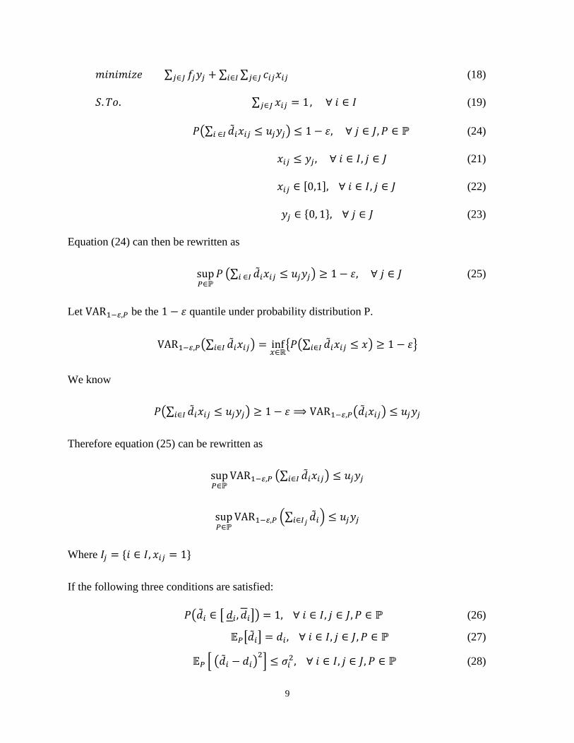
9
𝑚𝑖𝑛𝑖𝑚𝑖𝑧𝑒 ∑ 𝑓𝑗𝑦𝑗𝑗∈𝐽 + ∑ ∑ 𝑐𝑖𝑗𝑥𝑖𝑗𝑗∈𝐽𝑖∈𝐼 (18)
𝑆. 𝑇𝑜. ∑ 𝑥𝑖𝑗 = 1𝑗∈𝐽 , ∀ 𝑖 ∈ 𝐼 (19)
𝑃(∑ �̃�𝑖𝑥𝑖𝑗𝑖 ∈𝐼 ≤ 𝑢𝑗𝑦𝑗) ≤ 1 − 𝜀, ∀ 𝑗 ∈ 𝐽, 𝑃 ∈ ℙ (24)
𝑥𝑖𝑗 ≤ 𝑦𝑗 , ∀ 𝑖 ∈ 𝐼, 𝑗 ∈ 𝐽 (21)
𝑥𝑖𝑗 ∈ [0,1], ∀ 𝑖 ∈ 𝐼, 𝑗 ∈ 𝐽 (22)
𝑦𝑗 ∈ {0, 1}, ∀ 𝑗 ∈ 𝐽 (23)
Equation (24) can then be rewritten as
sup𝑃∈ℙ
𝑃 (∑ �̃�𝑖𝑥𝑖𝑗𝑖 ∈𝐼 ≤ 𝑢𝑗𝑦𝑗) ≥ 1 − 𝜀, ∀ 𝑗 ∈ 𝐽 (25)
Let VAR1−𝜀,𝑃 be the 1 − 𝜀 quantile under probability distribution P.
VAR1−𝜀,𝑃(∑ �̃�𝑖𝑥𝑖𝑗𝑖∈𝐼 ) = inf𝑥∈ℝ
{𝑃(∑ �̃�𝑖𝑥𝑖𝑗 ≤ 𝑥𝑖∈𝐼 ) ≥ 1 − 𝜀}
We know
𝑃(∑ �̃�𝑖𝑥𝑖𝑗 ≤ 𝑢𝑗𝑦𝑗𝑖∈𝐼 ) ≥ 1 − 𝜀 ⟹ VAR1−𝜀,𝑃(�̃�𝑖𝑥𝑖𝑗) ≤ 𝑢𝑗𝑦𝑗
Therefore equation (25) can be rewritten as
sup𝑃∈ℙ
VAR1−𝜀,𝑃 (∑ �̃�𝑖𝑥𝑖𝑗𝑖∈𝐼 ) ≤ 𝑢𝑗𝑦𝑗
sup𝑃∈ℙ
VAR1−𝜀,𝑃 (∑ �̃�𝑖𝑖∈𝐼𝑗) ≤ 𝑢𝑗𝑦𝑗
Where 𝐼𝑗 = {𝑖 ∈ 𝐼, 𝑥𝑖𝑗 = 1}
If the following three conditions are satisfied:
𝑃(�̃�𝑖 ∈ [ 𝑑𝑖, 𝑑𝑖]) = 1, ∀ 𝑖 ∈ 𝐼, 𝑗 ∈ 𝐽, 𝑃 ∈ ℙ (26)
𝔼𝑃[�̃�𝑖] = 𝑑𝑖 , ∀ 𝑖 ∈ 𝐼, 𝑗 ∈ 𝐽, 𝑃 ∈ ℙ (27)
𝔼𝑃 [ (�̃�𝑖 − 𝑑𝑖)2
] ≤ 𝜎𝑖2, ∀ 𝑖 ∈ 𝐼, 𝑗 ∈ 𝐽, 𝑃 ∈ ℙ (28)
10
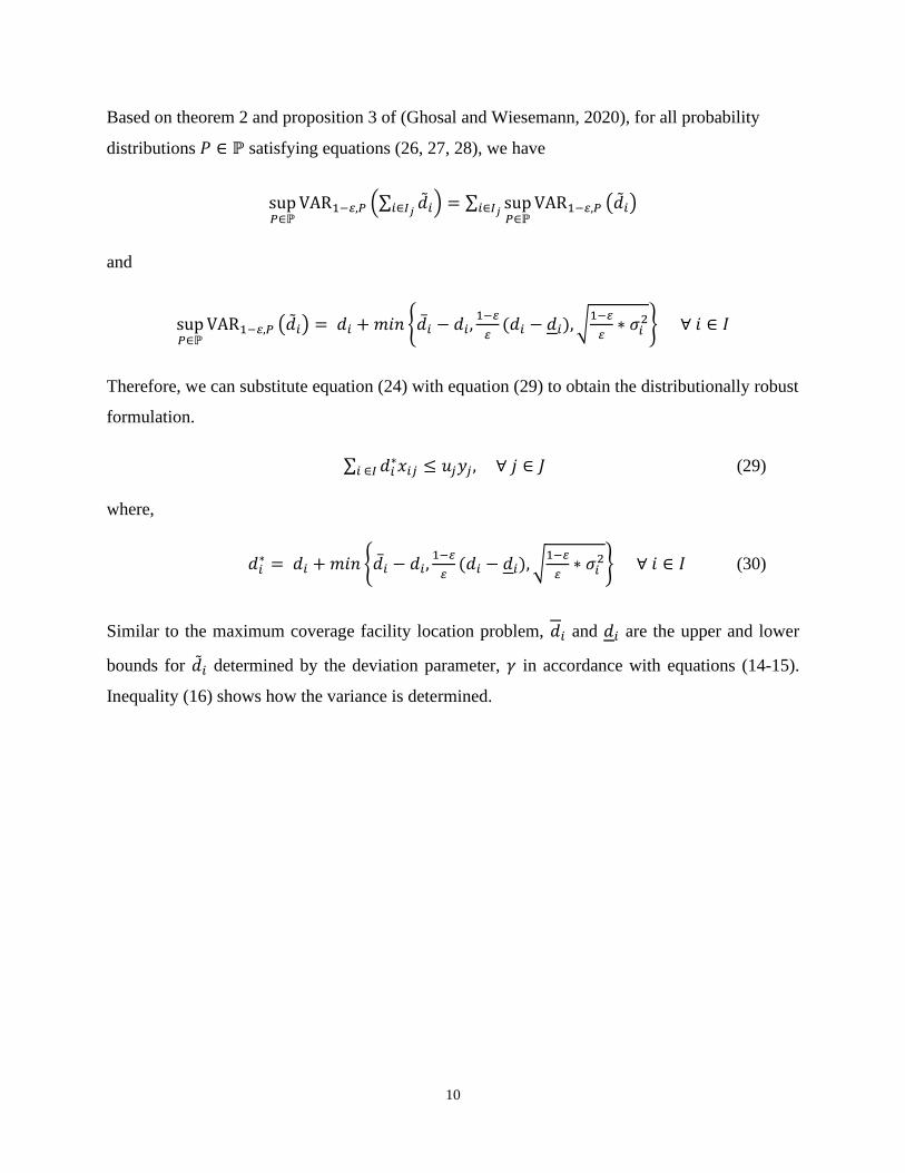
Based on theorem 2 and proposition 3 of (Ghosal and Wiesemann, 2020), for all probability
distributions 𝑃 ∈ ℙ satisfying equations (26, 27, 28), we have
sup𝑃∈ℙ
VAR1−𝜀,𝑃 (∑ �̃�𝑖𝑖∈𝐼𝑗) = ∑ sup
𝑃∈ℙVAR1−𝜀,𝑃 (�̃�𝑖)𝑖∈𝐼𝑗
and
sup𝑃∈ℙ
VAR1−𝜀,𝑃 (�̃�𝑖) = 𝑑𝑖 + 𝑚𝑖𝑛 {�̅�𝑖 − 𝑑𝑖,1−𝜀
𝜀(𝑑𝑖 − 𝑑𝑖), √
1−𝜀
𝜀∗ 𝜎𝑖
2} ∀ 𝑖 ∈ 𝐼
Therefore, we can substitute equation (24) with equation (29) to obtain the distributionally robust
formulation.
∑ 𝑑𝑖∗𝑥𝑖𝑗𝑖 ∈𝐼 ≤ 𝑢𝑗𝑦𝑗 , ∀ 𝑗 ∈ 𝐽 (29)
where,
𝑑𝑖∗ = 𝑑𝑖 + 𝑚𝑖𝑛 {�̅�𝑖 − 𝑑𝑖,
1−𝜀
𝜀(𝑑𝑖 − 𝑑𝑖), √
1−𝜀
𝜀∗ 𝜎𝑖
2} ∀ 𝑖 ∈ 𝐼 (30)
Similar to the maximum coverage facility location problem, 𝑑𝑖 and 𝑑𝑖 are the upper and lower
bounds for �̃�𝑖 determined by the deviation parameter, 𝛾 in accordance with equations (14-15).
Inequality (16) shows how the variance is determined.
11
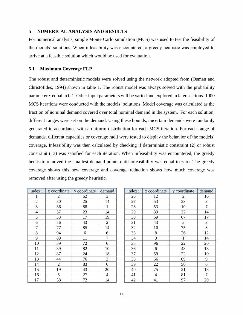
5 NUMERICAL ANALYSIS AND RESULTS
For numerical analysis, simple Monte Carlo simulation (MCS) was used to test the feasibility of
the models’ solutions. When infeasibility was encountered, a greedy heuristic was employed to
arrive at a feasible solution which would be used for evaluation.
5.1 Maximum Coverage FLP
The robust and deterministic models were solved using the network adopted from (Osman and
Christofides, 1994) shown in table 1. The robust model was always solved with the probability
parameter 𝜀 equal to 0.1. Other input parameters will be varied and explored in later sections. 1000
MCS iterations were conducted with the models’ solutions. Model coverage was calculated as the
fraction of nominal demand covered over total nominal demand in the system. For each solution,
different ranges were set on the demand. Using these bounds, uncertain demands were randomly
generated in accordance with a uniform distribution for each MCS iteration. For each range of
demands, different capacities or coverage radii were tested to display the behavior of the models’
coverage. Infeasibility was then calculated by checking if deterministic constraint (2) or robust
constraint (13) was satisfied for each iteration. When infeasibility was encountered, the greedy
heuristic removed the smallest demand points until infeasibility was equal to zero. The greedy
coverage shows this new coverage and coverage reduction shows how much coverage was
removed after using the greedy heuristic.
index i x coordinate y coordinate demand index i x coordinate y coordinate demand
1 2 62 3 26 12 2 16
2 80 25 14 27 53 33 3
3 36 88 1 28 53 10 7
4 57 23 14 29 33 32 14
5 33 17 19 30 69 67 17
6 76 43 2 31 43 5 3
7 77 85 14 32 10 75 3
8 94 6 6 33 8 26 12
9 89 11 7 34 3 1 14
10 59 72 6 35 96 22 20
11 39 82 10 36 6 48 13
12 87 24 18 37 59 22 10
13 44 76 3 38 66 69 9
14 2 83 6 39 22 50 6
15 19 43 20 40 75 21 18
16 5 27 4 41 4 81 7
17 58 72 14 42 41 97 20
12
18 14 50 11 43 92 34 9
19 43 18 19 44 12 64 1
20 87 7 15 45 60 84 8
21 11 56 15 46 35 100 5
22 31 16 4 47 38 2 1
23 51 94 13 48 9 9 7
24 55 13 13 49 54 59 9
25 84 57 5 50 1 58 2
Table 1: Network of Maximum Coverage FLP
5.1.1 Effect of Varying Capacity
For this analysis, an infinite coverage radius was assumed, and five facilities were located.
Capacity was tested between 70 and 140.
Model Capacity Demand
Range
Model
Coverage Infeasibility
Greedy
Coverage
Coverage
Reduction
Deterministic
70
[0.8d,1.2d]
0.714 0.965 0.68 0.035
80 0.816 0.982 0.784 0.032
90 0.918 0.964 0.888 0.031
100 1 0.924 0.981 0.019
110 1 0.91 0.978 0.022
120 1 0.917 0.977 0.023
130 1 0.885 0.983 0.017
140 1 0.886 0.981 0.019
70
[0,2d]
0.714 0.963 0.591 0.124
80 0.816 0.975 0.683 0.133
90 0.918 0.964 0.775 0.143
100 1 0.957 0.868 0.132
110 1 0.939 0.869 0.131
120 1 0.934 0.863 0.137
130 1 0.869 0.887 0.113
140 1 0.879 0.883 0.117
Robust
70
[0.8d,1.2d]
0.592 0 0.592 0
80 0.673 0 0.673 0
90 0.765 0 0.765 0
100 0.847 0 0.847 0
110 0.929 0 0.929 0
120 1 0 1 0
130 1 0 1 0
140 1 0 1 0
70 [0,2d] 0.357 0 0.357 0
13
80 0.408 0 0.408 0
90 0.459 0 0.459 0
100 0.51 0 0.51 0
110 0.561 0 0.561 0
120 0.612 0 0.612 0
130 0.663 0 0.663 0
140 0.714 0 0.714 0
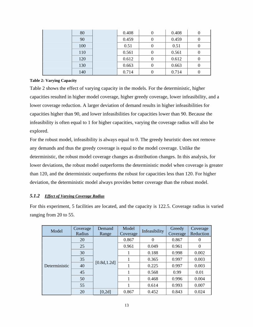
Table 2: Varying Capacity
Table 2 shows the effect of varying capacity in the models. For the deterministic, higher
capacities resulted in higher model coverage, higher greedy coverage, lower infeasibility, and a
lower coverage reduction. A larger deviation of demand results in higher infeasibilities for
capacities higher than 90, and lower infeasibilities for capacities lower than 90. Because the
infeasibility is often equal to 1 for higher capacities, varying the coverage radius will also be
explored.
For the robust model, infeasibility is always equal to 0. The greedy heuristic does not remove
any demands and thus the greedy coverage is equal to the model coverage. Unlike the
deterministic, the robust model coverage changes as distribution changes. In this analysis, for
lower deviations, the robust model outperforms the deterministic model when coverage is greater
than 120, and the deterministic outperforms the robust for capacities less than 120. For higher
deviation, the deterministic model always provides better coverage than the robust model.
5.1.2 Effect of Varying Coverage Radius
For this experiment, 5 facilities are located, and the capacity is 122.5. Coverage radius is varied
ranging from 20 to 55.
Model Coverage
Radius
Demand
Range
Model
Coverage Infeasibility
Greedy
Coverage
Coverage
Reduction
Deterministic
20
[0.8d,1.2d]
0.867 0 0.867 0
25 0.961 0.049 0.961 0
30 1 0.188 0.998 0.002
35 1 0.365 0.997 0.003
40 1 0.225 0.997 0.003
45 1 0.568 0.99 0.01
50 1 0.468 0.996 0.004
55 1 0.614 0.993 0.007
20 [0,2d] 0.867 0.452 0.843 0.024
14
25 0.961 0.679 0.911 0.05
30 1 0.728 0.941 0.059
35 1 0.788 0.928 0.072
40 1 0.829 0.919 0.081
45 1 0.72 0.932 0.068
50 1 0.707 0.952 0.048
55 1 0.751 0.935 0.065
Robust
20
[0.8d,1.2d]
0.845 0 0.845 0
25 0.918 0 0.918 0
30 0.973 0 0.973 0
35 1 0 1 0
20 [0,2d]
0.622 0 0.622 0
55 0.622 0 0.622 0
Table 3: Varying Coverage Radius
For the deterministic model there was more variation in the behavior of infeasibility, greedy
coverage, and coverage reduction as the coverage radius increased shown in table 3. This is
expected because the demand points which are available to a facility alter as the coverage radius
changes. In general, as the coverage radius increased, the infeasibility increased. The greedy
coverage also increased until coverage radius was equal to 30. For coverage radii greater than 30,
there was no significant change to greedy coverage or coverage reduction. A coverage radius of
30 produced the most optimal greedy coverage for both ranges of demand.
The robust model produced similar results as shown in section 5.1.1. The MCS shows no
infeasibility, and the greedy heuristic does not change the coverage. Using a larger variation
range of demands shows that coverage does not change as the coverage radius is increased from
20 to 55. For this analysis, the deterministic model always outperforms the robust model, expect
when the variation range of demand is less and the coverage radius is at least 35 units.
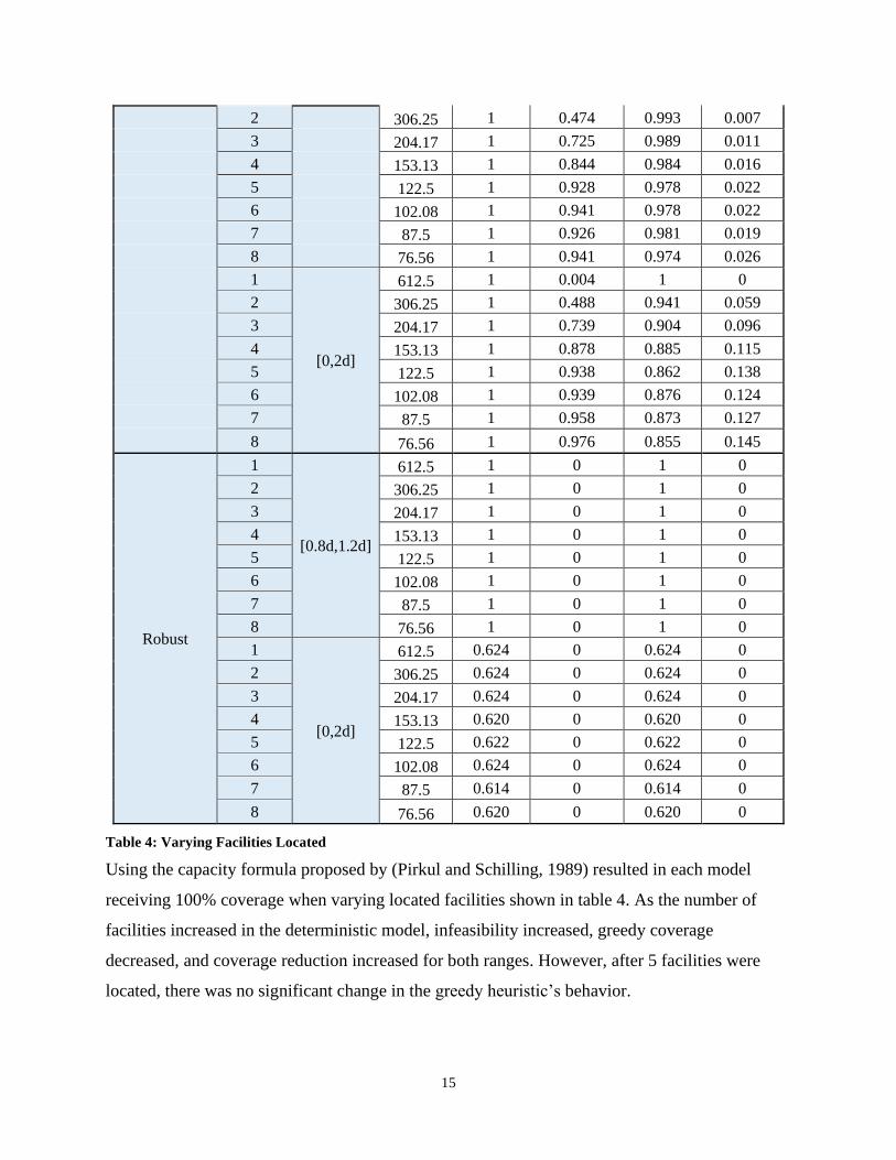
5.1.3 Effect of Varying Facilities Located
For this experiment, the number of facilities located ranges from 1 to 8, the capacity of each facility
is determined in accordance using the approximation proposed by (Pirkul and Schilling, 1989),
and an infinite coverage radius is considered.
Model Facilities Demand
Range Capacity
Model
Coverage Infeasibility
Greedy
Coverage
Coverage
Reduction
Deterministic 1 [0.8d,1.2d] 612.5 1 0 1 0
15
2 306.25 1 0.474 0.993 0.007
3 204.17 1 0.725 0.989 0.011
4 153.13 1 0.844 0.984 0.016
5 122.5 1 0.928 0.978 0.022
6 102.08 1 0.941 0.978 0.022
7 87.5 1 0.926 0.981 0.019
8 76.56 1 0.941 0.974 0.026
1
[0,2d]
612.5 1 0.004 1 0
2 306.25 1 0.488 0.941 0.059
3 204.17 1 0.739 0.904 0.096
4 153.13 1 0.878 0.885 0.115
5 122.5 1 0.938 0.862 0.138
6 102.08 1 0.939 0.876 0.124
7 87.5 1 0.958 0.873 0.127
8 76.56 1 0.976 0.855 0.145
Robust
1
[0.8d,1.2d]
612.5 1 0 1 0
2 306.25 1 0 1 0
3 204.17 1 0 1 0
4 153.13 1 0 1 0
5 122.5 1 0 1 0
6 102.08 1 0 1 0
7 87.5 1 0 1 0
8 76.56 1 0 1 0
1
[0,2d]
612.5 0.624 0 0.624 0
2 306.25 0.624 0 0.624 0
3 204.17 0.624 0 0.624 0
4 153.13 0.620 0 0.620 0
5 122.5 0.622 0 0.622 0
6 102.08 0.624 0 0.624 0
7 87.5 0.614 0 0.614 0
8 76.56 0.620 0 0.620 0
Table 4: Varying Facilities Located
Using the capacity formula proposed by (Pirkul and Schilling, 1989) resulted in each model
receiving 100% coverage when varying located facilities shown in table 4. As the number of
facilities increased in the deterministic model, infeasibility increased, greedy coverage
decreased, and coverage reduction increased for both ranges. However, after 5 facilities were
located, there was no significant change in the greedy heuristic’s behavior.
16
The robust model provides as much model coverage as the deterministic for small ranges of
demand, and significantly less model coverage for large ranges of demand. For this analysis, the
robust can outperform the deterministic by providing complete coverage with no infeasibility if
small range distributions of demand can be expected. For large ranges of demand, the
deterministic model is preferred.
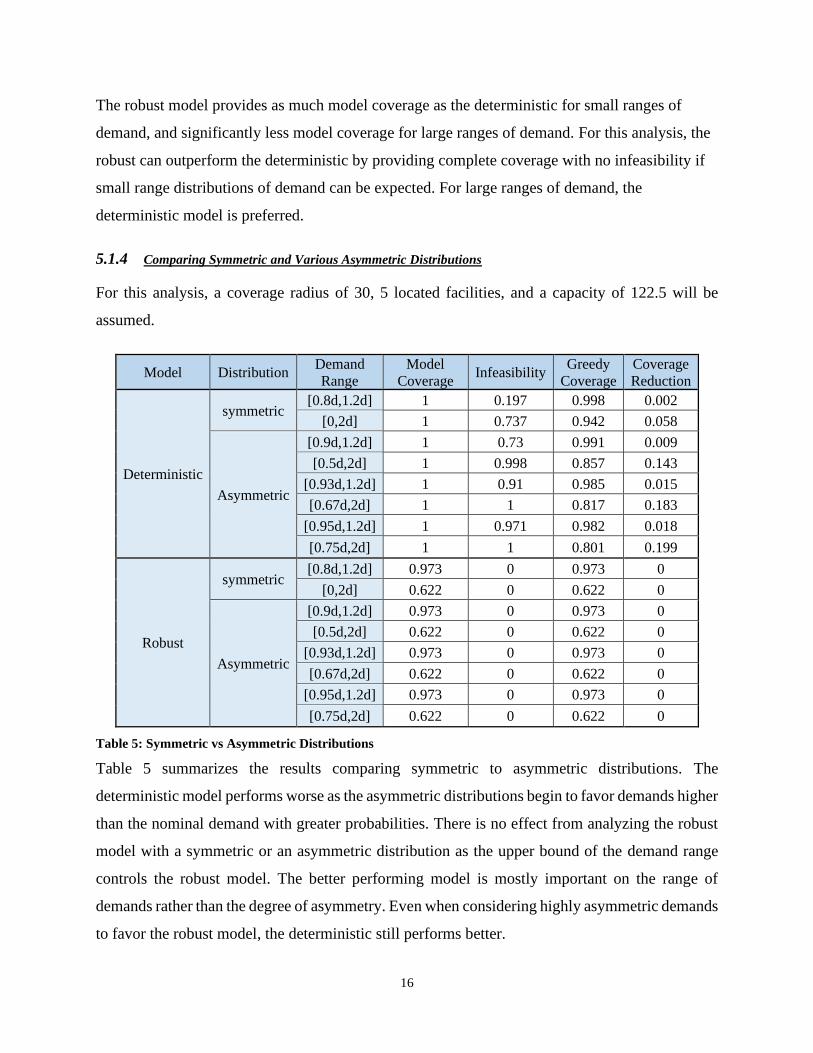
5.1.4 Comparing Symmetric and Various Asymmetric Distributions
For this analysis, a coverage radius of 30, 5 located facilities, and a capacity of 122.5 will be
assumed.
Model Distribution Demand
Range
Model
Coverage Infeasibility
Greedy
Coverage
Coverage
Reduction
Deterministic
symmetric [0.8d,1.2d] 1 0.197 0.998 0.002
[0,2d] 1 0.737 0.942 0.058
Asymmetric
[0.9d,1.2d] 1 0.73 0.991 0.009
[0.5d,2d] 1 0.998 0.857 0.143
[0.93d,1.2d] 1 0.91 0.985 0.015
[0.67d,2d] 1 1 0.817 0.183
[0.95d,1.2d] 1 0.971 0.982 0.018
[0.75d,2d] 1 1 0.801 0.199
Robust
symmetric [0.8d,1.2d] 0.973 0 0.973 0
[0,2d] 0.622 0 0.622 0
Asymmetric
[0.9d,1.2d] 0.973 0 0.973 0
[0.5d,2d] 0.622 0 0.622 0
[0.93d,1.2d] 0.973 0 0.973 0
[0.67d,2d] 0.622 0 0.622 0
[0.95d,1.2d] 0.973 0 0.973 0
[0.75d,2d] 0.622 0 0.622 0
Table 5: Symmetric vs Asymmetric Distributions
Table 5 summarizes the results comparing symmetric to asymmetric distributions. The
deterministic model performs worse as the asymmetric distributions begin to favor demands higher
than the nominal demand with greater probabilities. There is no effect from analyzing the robust
model with a symmetric or an asymmetric distribution as the upper bound of the demand range
controls the robust model. The better performing model is mostly important on the range of
demands rather than the degree of asymmetry. Even when considering highly asymmetric demands
to favor the robust model, the deterministic still performs better.
17
5.1.5 Maximum Coverage FLP Discussion
The results in tables 2, 3, and 4 identify that when complete coverage cannot be achieved, the
deterministic solution provides more coverage across a range of capacities, coverage radii, or
located facilities, and various deviations of �̃�𝑖. The capacity approximation to reach complete
coverage proposed by (Pirkul and Schilling, 1989) is 122.5 when 5 facilities are located. It is not
surprising that when capacity is above 120 for 5 located facilities, complete coverage is achieved,
and the robust model performs better. Because the robust model is generated using the bounds of
�̃�𝑖, it provides a better mapping of variables compared with the deterministic. However, exploring
different coverage radii and located facilities shows that even when a capacity of 122.5 is assumed,
the deterministic model performs better until coverage radius equals 35.
The comparison of symmetric to asymmetric distributions in table 5 showed how much better the
deterministic is as providing coverage under a practical coverage radius of 30. Even when
considering very unlikely worst case asymmetric distributions, it is still observed that the
deterministic performs better at providing maximum coverage. In practical application of FLPs,
an infinite coverage radius would likely not be considered. However, there are other networks
which could be explored with this formulation and there are scenarios in which coverage radius is
not such an important factor.
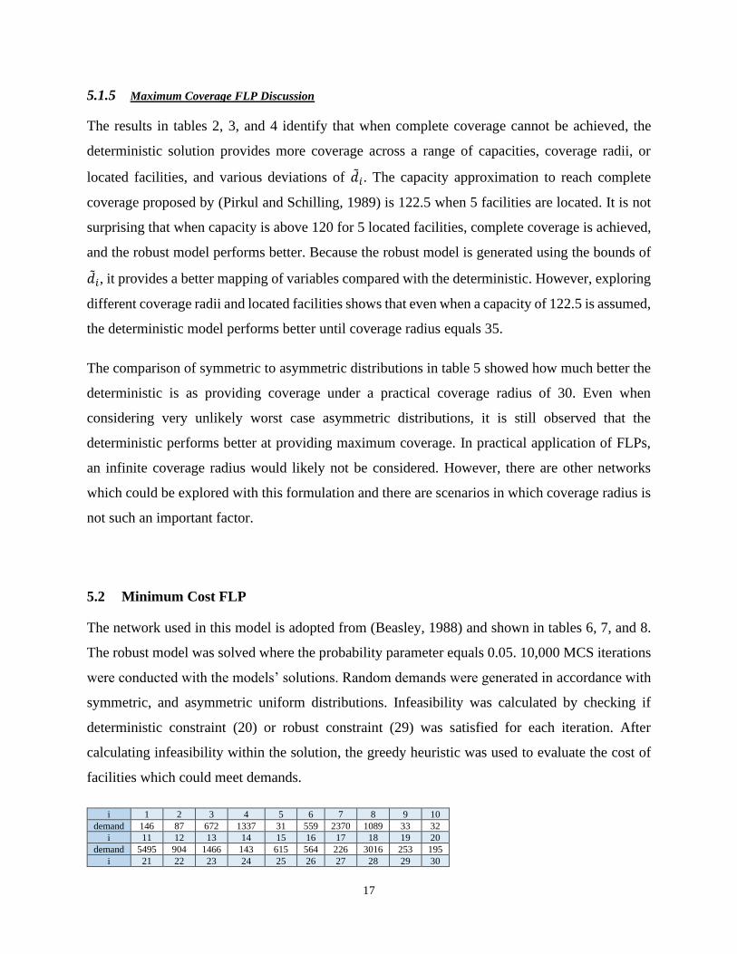
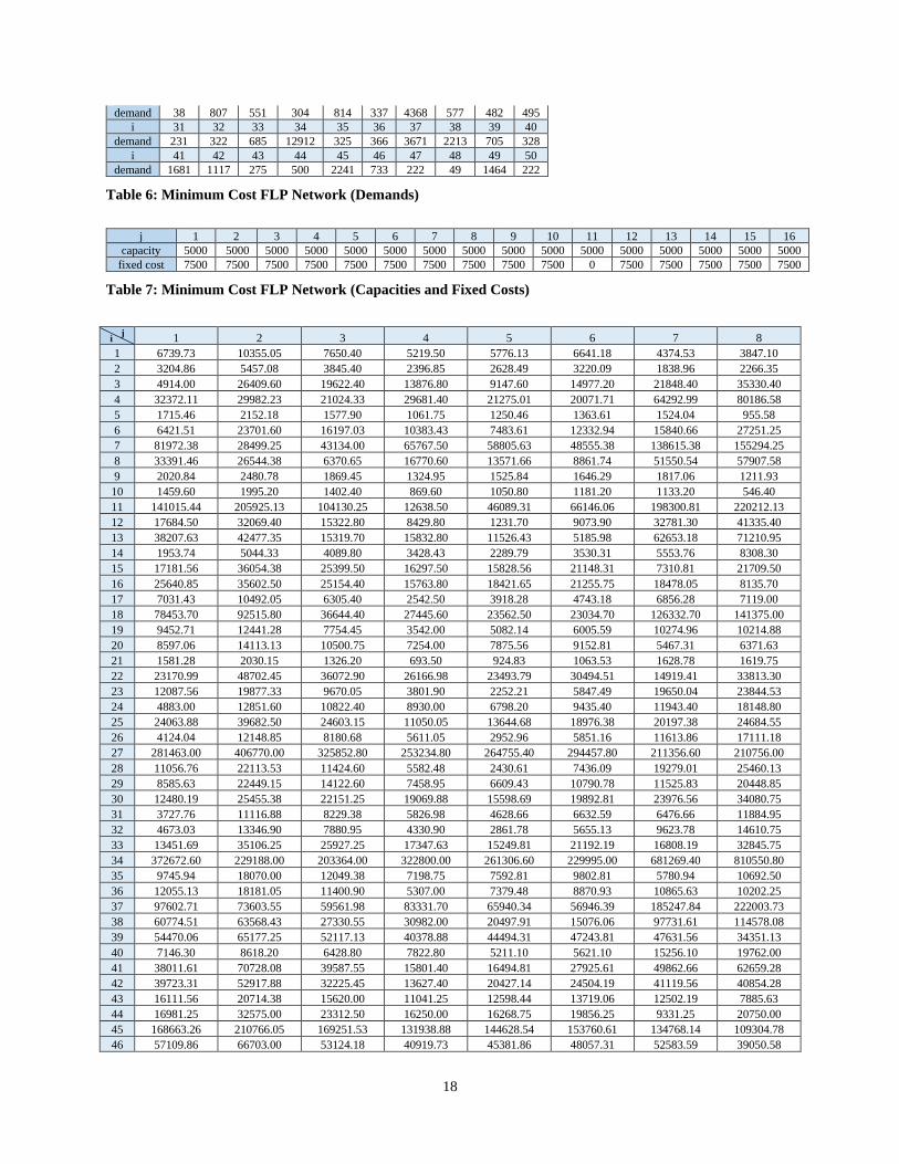
5.2 Minimum Cost FLP
The network used in this model is adopted from (Beasley, 1988) and shown in tables 6, 7, and 8.
The robust model was solved where the probability parameter equals 0.05. 10,000 MCS iterations
were conducted with the models’ solutions. Random demands were generated in accordance with
symmetric, and asymmetric uniform distributions. Infeasibility was calculated by checking if
deterministic constraint (20) or robust constraint (29) was satisfied for each iteration. After
calculating infeasibility within the solution, the greedy heuristic was used to evaluate the cost of
facilities which could meet demands.
i 1 2 3 4 5 6 7 8 9 10
demand 146 87 672 1337 31 559 2370 1089 33 32
i 11 12 13 14 15 16 17 18 19 20
demand 5495 904 1466 143 615 564 226 3016 253 195
i 21 22 23 24 25 26 27 28 29 30
18
demand 38 807 551 304 814 337 4368 577 482 495
i 31 32 33 34 35 36 37 38 39 40
demand 231 322 685 12912 325 366 3671 2213 705 328
i 41 42 43 44 45 46 47 48 49 50
demand 1681 1117 275 500 2241 733 222 49 1464 222
Table 6: Minimum Cost FLP Network (Demands)
j 1 2 3 4 5 6 7 8 9 10 11 12 13 14 15 16
capacity 5000 5000 5000 5000 5000 5000 5000 5000 5000 5000 5000 5000 5000 5000 5000 5000
fixed cost 7500 7500 7500 7500 7500 7500 7500 7500 7500 7500 0 7500 7500 7500 7500 7500
Table 7: Minimum Cost FLP Network (Capacities and Fixed Costs)
i j 1 2 3 4 5 6 7 8
1 6739.73 10355.05 7650.40 5219.50 5776.13 6641.18 4374.53 3847.10
2 3204.86 5457.08 3845.40 2396.85 2628.49 3220.09 1838.96 2266.35
3 4914.00 26409.60 19622.40 13876.80 9147.60 14977.20 21848.40 35330.40
4 32372.11 29982.23 21024.33 29681.40 21275.01 20071.71 64292.99 80186.58
5 1715.46 2152.18 1577.90 1061.75 1250.46 1363.61 1524.04 955.58
6 6421.51 23701.60 16197.03 10383.43 7483.61 12332.94 15840.66 27251.25
7 81972.38 28499.25 43134.00 65767.50 58805.63 48555.38 138615.38 155294.25
8 33391.46 26544.38 6370.65 16770.60 13571.66 8861.74 51550.54 57907.58
9 2020.84 2480.78 1869.45 1324.95 1525.84 1646.29 1817.06 1211.93
10 1459.60 1995.20 1402.40 869.60 1050.80 1181.20 1133.20 546.40
11 141015.44 205925.13 104130.25 12638.50 46089.31 66146.06 198300.81 220212.13
12 17684.50 32069.40 15322.80 8429.80 1231.70 9073.90 32781.30 41335.40
13 38207.63 42477.35 15319.70 15832.80 11526.43 5185.98 62653.18 71210.95
14 1953.74 5044.33 4089.80 3428.43 2289.79 3530.31 5553.76 8308.30
15 17181.56 36054.38 25399.50 16297.50 15828.56 21148.31 7310.81 21709.50
16 25640.85 35602.50 25154.40 15763.80 18421.65 21255.75 18478.05 8135.70
17 7031.43 10492.05 6305.40 2542.50 3918.28 4743.18 6856.28 7119.00
18 78453.70 92515.80 36644.40 27445.60 23562.50 23034.70 126332.70 141375.00
19 9452.71 12441.28 7754.45 3542.00 5082.14 6005.59 10274.96 10214.88
20 8597.06 14113.13 10500.75 7254.00 7875.56 9152.81 5467.31 6371.63
21 1581.28 2030.15 1326.20 693.50 924.83 1063.53 1628.78 1619.75
22 23170.99 48702.45 36072.90 26166.98 23493.79 30494.51 14919.41 33813.30
23 12087.56 19877.33 9670.05 3801.90 2252.21 5847.49 19650.04 23844.53
24 4883.00 12851.60 10822.40 8930.00 6798.20 9435.40 11943.40 18148.80
25 24063.88 39682.50 24603.15 11050.05 13644.68 18976.38 20197.38 24684.55
26 4124.04 12148.85 8180.68 5611.05 2952.96 5851.16 11613.86 17111.18
27 281463.00 406770.00 325852.80 253234.80 264755.40 294457.80 211356.60 210756.00
28 11056.76 22113.53 11424.60 5582.48 2430.61 7436.09 19279.01 25460.13
29 8585.63 22449.15 14122.60 7458.95 6609.43 10790.78 11525.83 20448.85
30 12480.19 25455.38 22151.25 19069.88 15598.69 19892.81 23976.56 34080.75
31 3727.76 11116.88 8229.38 5826.98 4628.66 6632.59 6476.66 11884.95
32 4673.03 13346.90 7880.95 4330.90 2861.78 5655.13 9623.78 14610.75
33 13451.69 35106.25 25927.25 17347.63 15249.81 21192.19 16808.19 32845.75
34 372672.60 229188.00 203364.00 322800.00 261306.60 229995.00 681269.40 810550.80
35 9745.94 18070.00 12049.38 7198.75 7592.81 9802.81 5780.94 10692.50
36 12055.13 18181.05 11400.90 5307.00 7379.48 8870.93 10865.63 10202.25
37 97602.71 73603.55 59561.98 83331.70 65940.34 56946.39 185247.84 222003.73
38 60774.51 63568.43 27330.55 30982.00 20497.91 15076.06 97731.61 114578.08
39 54470.06 65177.25 52117.13 40378.88 44494.31 47243.81 47631.56 34351.13
40 7146.30 8618.20 6428.80 7822.80 5211.10 5621.10 15256.10 19762.00
41 38011.61 70728.08 39587.55 15801.40 16494.81 27925.61 49862.66 62659.28
42 39723.31 52917.88 32225.45 13627.40 20427.14 24504.19 41119.56 40854.28
43 16111.56 20714.38 15620.00 11041.25 12598.44 13719.06 12502.19 7885.63
44 16981.25 32575.00 23312.50 16250.00 16268.75 19856.25 9331.25 20750.00
45 168663.26 210766.05 169251.53 131938.88 144628.54 153760.61 134768.14 109304.78
46 57109.86 66703.00 53124.18 40919.73 45381.86 48057.31 52583.59 39050.58
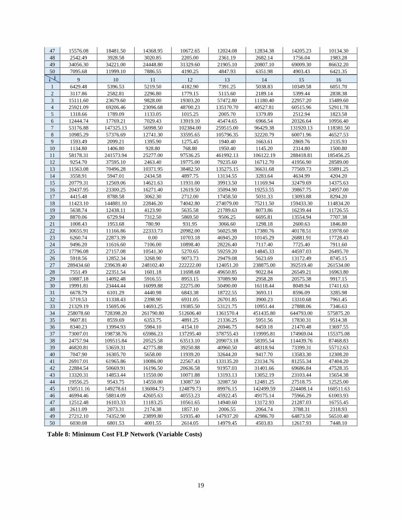
19
47 15576.08 18481.50 14368.95 10672.65 12024.08 12834.38 14205.23 10134.30
48 2542.49 3928.58 3020.85 2205.00 2361.19 2682.14 1756.04 1983.28
49 34056.30 34221.00 24448.80 31329.60 21905.10 20807.10 69009.30 86632.20
50 7095.68 11999.10 7886.55 4190.25 4847.93 6351.98 4903.43 6421.35
i j 9 10 11 12 13 14 15 16
1 6429.48 5396.53 5219.50 4182.90 7391.25 5038.83 10349.58 6051.70
2 3117.86 2582.81 2296.80 1779.15 5115.60 2189.14 5399.44 2838.38
3 15111.60 23679.60 9828.00 19303.20 57472.80 11180.40 22957.20 15489.60
4 25921.09 69206.46 23096.68 48700.23 135170.70 40527.81 60515.96 52911.78
5 1318.66 1789.09 1133.05 1015.25 2005.70 1379.89 2512.94 1823.58
6 12444.74 17769.21 7029.43 13919.10 45474.65 6966.54 20326.64 10956.40
7 53176.88 147325.13 56998.50 102384.00 259515.00 96429.38 131920.13 118381.50
8 10985.29 57376.69 12741.30 33595.65 105796.35 32220.79 60071.96 46527.53
9 1593.49 2099.21 1395.90 1275.45 1940.40 1663.61 2869.76 2135.93
10 1134.80 1406.80 928.80 768.80 1950.40 1145.20 2314.80 1500.80
11 58178.31 241573.94 25277.00 97536.25 461992.13 106122.19 288418.81 185456.25
12 9254.70 37595.10 2463.40 19775.00 79235.60 16712.70 41956.90 28589.00
13 11563.08 70496.28 10371.95 38482.50 135275.15 36631.68 77569.73 55891.25
14 3558.91 5947.01 2434.58 4897.75 13134.55 3283.64 4634.99 4204.20
15 20779.31 12569.06 14621.63 11931.00 39913.50 11169.94 32479.69 14375.63
16 20437.95 23300.25 16271.40 12619.50 35094.90 19253.55 39867.75 24957.00
17 4415.48 8788.58 3062.30 2712.00 17458.50 5031.33 13093.88 8294.20
18 11423.10 144881.10 22846.20 74042.80 274079.00 75211.50 159433.30 114834.20
19 5638.74 12438.11 4123.90 5635.58 21789.63 8073.86 16239.44 11726.55
20 8870.06 6729.94 7312.50 5869.50 9506.25 6695.81 13554.94 7707.38
21 1008.43 1953.68 780.90 931.95 3066.60 1298.18 2600.63 1846.80
22 30655.91 11166.86 22333.73 20982.00 56025.98 17380.76 40178.51 15978.60
23 6260.74 22873.39 0.00 10703.18 46945.20 10145.29 26881.91 17728.43
24 9496.20 11616.60 7106.00 10898.40 28226.40 7117.40 7725.40 7911.60
25 17796.08 27157.08 10541.30 5270.65 59259.20 14845.33 44597.03 26495.70
26 5918.56 12852.34 3268.90 9073.73 29479.08 5623.69 13172.49 8745.15
27 289434.60 239639.40 248102.40 222222.00 124051.20 238875.00 392519.40 261534.00
28 7551.49 22351.54 1601.18 11698.68 49650.85 9022.84 26549.21 16963.80
29 10887.18 14092.48 5916.55 8953.15 37089.90 2958.28 20575.38 9917.15
30 19991.81 23444.44 16099.88 22275.00 50490.00 16118.44 8049.94 17411.63
31 6678.79 6101.29 4440.98 6843.38 18722.55 3693.11 8596.09 3285.98
32 5719.53 11338.43 2398.90 6931.05 26701.85 3900.23 13310.68 7961.45
33 21329.19 15695.06 14693.25 19385.50 53121.75 10951.44 27888.06 7346.63
34 258078.60 728398.20 261790.80 512606.40 1361570.4 451435.80 644793.00 575875.20
35 9607.81 8559.69 6353.75 4891.25 21336.25 5951.56 17830.31 9514.38
36 8340.23 13994.93 5984.10 4154.10 26946.75 8459.18 21470.48 13697.55
37 73007.01 198738.76 65986.23 137295.40 378755.43 119995.81 174969.04 155375.08
38 24757.94 109515.84 20525.58 63513.10 209073.18 58395.54 114439.76 87468.83
39 46820.81 53659.31 42775.88 39250.88 40960.50 48318.94 73399.31 55712.63
40 7047.90 16305.70 5658.00 11939.20 32644.20 9417.70 13583.30 12308.20
41 26917.01 61965.86 10086.00 22567.43 133135.20 23134.76 81255.34 47404.20
42 22884.54 50669.91 16196.50 20636.58 91957.03 31401.66 69686.84 47528.35
43 13320.31 14853.44 11550.00 10071.88 13193.13 13052.19 23103.44 15654.38
44 19556.25 9543.75 14550.00 13087.50 32087.50 12481.25 27518.75 12525.00
45 150511.16 149278.61 136084.73 124879.73 89976.15 142499.59 224408.14 160511.63
46 46994.46 58814.09 42605.63 40553.23 45922.45 49175.14 75966.29 61003.93
47 12512.48 16103.33 11183.25 10561.65 14940.60 13172.93 21287.03 16755.45
48 2611.09 2073.31 2174.38 1857.10 2006.55 2064.74 3788.31 2318.93
49 27212.10 74352.90 23899.80 51935.40 147937.20 42986.70 64873.50 56510.40
50 6030.08 6801.53 4001.55 2614.05 14979.45 4503.83 12617.93 7448.10
Table 8: Minimum Cost FLP Network (Variable Costs)
20
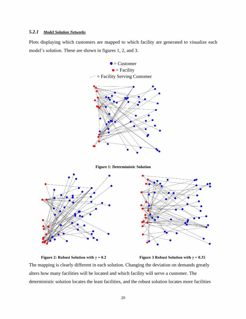
5.2.1 Model Solution Networks
Plots displaying which customers are mapped to which facility are generated to visualize each
model’s solution. These are shown in figures 1, 2, and 3.
= Customer
= Facility
= Facility Serving Customer
Figure 1: Deterministic Solution
Figure 2: Robust Solution with γ = 0.2 Figure 3 Robust Solution with γ = 0.35
The mapping is clearly different in each solution. Changing the deviation on demands greatly
alters how many facilities will be located and which facility will serve a customer. The
deterministic solution locates the least facilities, and the robust solution locates more facilities
21
when given greater deviations. For this network of 16 potential facilities, the deterministic model
located 13, the robust model with γ = 0.2 located 15, and the robust model with γ = 0.35 located
16.
5.2.2 MCS Results Considering Symmetric and Asymmetric Distributions
The robust and deterministic models were solved using the input network and parameters outlined
in section 5.2.
Model Distribution Demand
Range
Objective
Value Infeasibility Greedy Cost
Change in
Cost
Deterministic
Symmetric [0.8d,1.2d] $1,040,444.38 0.9943 $925,048.35 -$115,396.02
[0.65d,1.35d] $1,040,444.38 0.9940 $898,010.44 -$142,433.93
Asymmetric [0.9d,1.2d] $1,040,444.38 1 $877,468.04 -$162,976.33
[0.825d,1.35d] $1,040,444.38 1 $840,784.51 -$199,659.87
Robust
Symmetric [0.8d,1.2d] $1,183,964.33 0 $1,183,964.33 $0.00
[0.65d,1.35d] $1,336,767.35 0 $1,336,767.35 $0.00
Asymmetric [0.9d,1.2d] $1,183,964.33 0 $1,183,964.33 $0.00
[0.825d,1.35d] $1,336,767.35 0 $1,336,767.35 $0.00
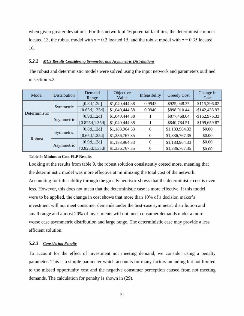
Table 9: Minimum Cost FLP Results
Looking at the results from table 9, the robust solution consistently costed more, meaning that
the deterministic model was more effective at minimizing the total cost of the network.
Accounting for infeasibility through the greedy heuristic shows that the deterministic cost is even
less. However, this does not mean that the deterministic case is more effective. If this model
were to be applied, the change in cost shows that more than 10% of a decision maker’s
investment will not meet consumer demands under the best-case symmetric distribution and
small range and almost 20% of investments will not meet consumer demands under a more
worse case asymmetric distribution and large range. The deterministic case may provide a less
efficient solution.
5.2.3 Considering Penalty
To account for the effect of investment not meeting demand, we consider using a penalty
parameter. This is a simple parameter which accounts for many factors including but not limited
to the missed opportunity cost and the negative consumer perception caused from not meeting
demands. The calculation for penalty is shown in (29).
22
∑ 𝑓𝑦𝑗𝑗∈𝐽 + ∑ ∑ 𝑐𝑖𝑗�̃�𝑖𝑗𝑗∈𝐽𝑖∈𝐼 + ∑ ∑ 𝜌�̃�𝑖(𝑥𝑖𝑗 − �̃�𝑖𝑗)𝑗∈𝐽𝑖∈𝐼 (29)
where,
𝜌 = penalty
�̃�𝑖𝑗 = 𝑥𝑖𝑗 after the greedy heuristic
Demand Range Penalty Cost after greedy
heuristic Change in Cost
[0.8d,1.2d] 0 $925,048.35 -$115,396.02
[0.65d,1.35d] 0 $898,010.44 -$142,433.93
[0.8d,1.2d] 25 $1,158,736.63 $118,292.25
[0.65d,1.35d] 25 $1,165,224.90 $124,780.53
[0.8d,1.2d] 50 $1,393,468.75 $353,024.37
[0.65d,1.35d] 50 $1,425,226.54 $384,728.16
Table 10: Effect of Considering Penalty
Table 10 shows the effects of various penalties on the deterministic model’s performance. The
true value of penalty is unknown and varies based on location, products, market, and consumers.
Because of this, a range of penalties are evaluated to capture these fluctuations. For penalties
greater than 25, the robust model outperforms the deterministic.
5.2.4 Minimum Cost FLP Discussion
The results in table 7 show that the deterministic solution provides a lower cost. However, it is not
realistic to consider this lower cost as better with 99.4% infeasibility in the model. We are almost
completely certain that some demands will not be covered. For a symmetric, uniform deviation of
0.2, uncovered demands make up 11.1% of the objective cost and for a symmetric, uniform
deviation of 0.35, uncovered demands make up 13.7% of the objective cost. To rebalance the
results, a penalty is added to account for shortages and lost opportunity cost. The penalty can vary
based on local demands and prices, so table 10 shows results considering a range of values for
penalty. It becomes clear that the penalty from not meeting demands can easily cause the robust
model to outperform the deterministic.
23
5.3 Evaluation of 𝒅𝒊∗
In the maximum coverage FLP, constraint (8) is satisfied with a probability of 1. The reason that
a lower confidence was not produced is because of how 𝑑𝑖∗ is evaluated from the second term in
equation (13). For the demands and probability parameter used, the first entry of the minimum
statement in (13) always controls. The result is that 𝑑𝑖∗ is equal to �̅�𝑖 for the demands used in this
problem. Similarly, in the minimum cost FLP, constraint (24) is satisfied with a probability of 1,
and thus 𝑑𝑖∗ is equal to �̅�𝑖.
This result may be too conservative. While having 𝑑𝑖∗ equal to �̅�𝑖 does satisfy the constraints of (8)
and (24), the initial goal was to have a parameter which could provide an upper limit for �̃�𝑖 without
using the upper bound. Doing so would cause a small amount infeasibility in the MCS and
ultimately a more optimal solution.
24
6 CONCLUSION
FLPs are network problems in which facilities are located to optimally meet objectives while
satisfying constraints. Objectives and constraints vary based on the model’s application to meet
certain goals. The objective of minimizing cost is used in the private sector because reducing cost
is directly correlated to maximizing asset utilization. Public sector applications include postal
services, waste management, fire departments, police, and others. Maximizing coverage is a better
objective to suit these applications because they provide essential services. For any FLP, the
constraints are modeled to provide more control of the objective.
The two models considered in this paper, the minimum cost FLP and maximum coverage FLP, are
archetypal examples of problems which have been popular in private or public sector applications.
The constraints for the minimum cost FLP suit the idea of maximizing asset utilization because
demands can be fractionally covered. The constraints for the maximum coverage FLP include a
coverage radius, number of facilities to locate, and a binary decision variable to cover demands.
These constraints also better fit the objective by giving more control over how coverage can be
maximized.
Even with this effort, these models are both deterministic, and their solutions can only be accurate
with accurate assumptions. However, parameters like demand, capacity, and cost are never exact.
Natural market fluctuations and extreme events will always cause these parameters to deviate. To
get a better picture of each problem, robust problems can be developed for both the maximum
coverage FLP and minimum cost FLP by considering each demand as uncertain.
The methods by which the robust FLPs were developed in this paper provided convenient and fast
computations. The deterministic maximum covering FLP provided better coverage when
considering more common input parameters. However, there exist scenarios where the robust
model performs better than the deterministic. The minimum cost FLP initially shows that the
deterministic performs better than the robust. However, the deterministic solution was highly
infeasible and penalty considerations show that the robust can easily outperform the deterministic.
For both problems and networks, the equivalent uncertain demand 𝑑𝑖∗ used in formulation was
equal to the upper bound set by deviation. Other networks and problems should be explored to find
scenarios where 𝑑𝑖∗ is not always equal to the upper bound.
25
7 REFERENCES
1. “Code of Ethics.” American Society of Civil Engineers (ASCE), www.asce.org/code-of-ethics/.
2. Church, R., and ReVell, C. (1974). “The maximal covering facility location problem.” Papers of
the Regional Science Association, 32(1), 101-118.
3. Current, J., Daskin, M., and Schilling, D. (2002). “Discrete network location models.” Facility
location: Applications and theory, 1, 81-118.
4. Esnaf, Ş., and Küçükdeniz, T. (2009). “A fuzzy clustering-based hybrid method for a multi-facility
location problem.” Journal of Intelligent Manufacturing, 20(2), 259-265.
5. Arabani, A. B., and Farahani, R. Z. (2012). “Facility location dynamics: An overview of
classifications and applications.” Computers & Industrial Engineering, 62(1), 408-420.
6. Chauhan, D., Unnikrishnan, A., and Figliozzi, M. (2019). “Maximum coverage capacitated facility
location problem with range constrained drones.” Transportation Research Part C: Emerging
Technologies, 99, 1-18.
7. Karatas, M., and Dasci, A. (2020). “A two-level facility location and sizing problem for maximal
coverage.” Computers & Industrial Engineering, 139, 106204.
8. Arslan, O. (2021). “The location-or-routing problem.” Transportation Research Part B:
Methodological, 147, 1-21.
9. Snyder, L. (2006). “Facility location under uncertainty: a review.” IIE transactions, 38(7), 547-
564.
10. Snyder, L. V., and Daskin, M. S. (2005). “Reliability models for facility location: the expected
failure cost case.” Transportation Science, 39(3), 400-416.
11. Bertsimas, D., and Sim, M. (2004). “The price of robustness.” Operations research, 52(1), 35-53.
12. Wang, Q., Batta, R., and Rump, C. M. (2002). “Algorithms for a facility location problem with
stochastic customer demand and immobile servers.” Annals of operations Research, 111(1), 17-
34.
13. Miranda, P. A., and Garrido, R. A. (2004). “Incorporating inventory control decisions into a
strategic distribution network design model with stochastic demand.” Transportation Research
Part E: Logistics and Transportation Review, 40(3), 183-207.
14. Baron, O., Milner, J., and Naseraldin, H. (2011). “Facility location: A robust optimization
approach.” Production and Operations Management, 20(5), 772-785.
15. Gülpınar, N., Pachamanova, D., and Çanakoğlu, E. (2013). “Robust strategies for facility location
under uncertainty.” European Journal of Operational Research, 225(1), 21-35.
16. Naoum-Sawaya, J., and S. Elhedhli, S. (2013). “A stochastic optimization model for real-time
ambulance redeployment.” Computers & Operations Research, 40(8), 1972-1978.
26
17. Berglund, P. G., and Kwon, C. (2014). “Robust facility location problem for hazardous waste
transportation.” Networks and spatial Economics, 14(1), 91-116.
18. Lutter, P., Degel, D., Büsing, C., Koster, A., and Werners B., (2017). “Improved handling of
uncertainty and robustness in set covering problems.” European Journal of Operational Research,
263(1), 35-49.
19. Zhong, S., Cheng, R., Jiang, Y., Wang, Z., Larsen, A., and Nielsen, O. A. (2020). “Risk-averse
optimization of disaster relief facility location and vehicle routing under stochastic
demand.” Transportation Research Part E: Logistics and Transportation Review, 141, 102015.
20. Chauhan, D. R., Unnikrishnan, A., Figliozzi, M., and Boyles, S. D. (2020). “Robust maximum
coverage facility location problem with drones considering uncertainties in battery availability and
consumption.” Transportation Research Record, 2675(2) 25–39.
21. Basciftci, B., Ahmed, S., and Shen, S. (2021). Distributionally robust facility location problem
under decision-dependent stochastic demand. European Journal of Operational Research, 292(2),
548-561.
22. Ghosal, S., and Wiesemann, W. (2020). “The distributionally robust chance constrained vehicle
routing problem.” Operations Research, 68(3), 716-732.
23. Bhatia, R., and Davis, C., (2000) “A better bound on the variance.” The American Mathematical
Monthly, 107(4):353–357.
24. Beasley, J., (1988). “An algorithm for solving large capacitated warehouse location problems.”
European Journal of Operational Research, 33, 314-325.
25. Osman, I.H., and Christofides, N. (1994). “Capacitated clustering problems by hybrid simulated
annealing and tabu search.” International Transactions in Operational Research, 1(3): 317-336.
26. Pirkul, H., and Schilling, D. (1989). “The capacitated maximal covering location problem with
backup service.” Annals of Operations Research, 18(1), 141-154.

27
8 APPENDIX
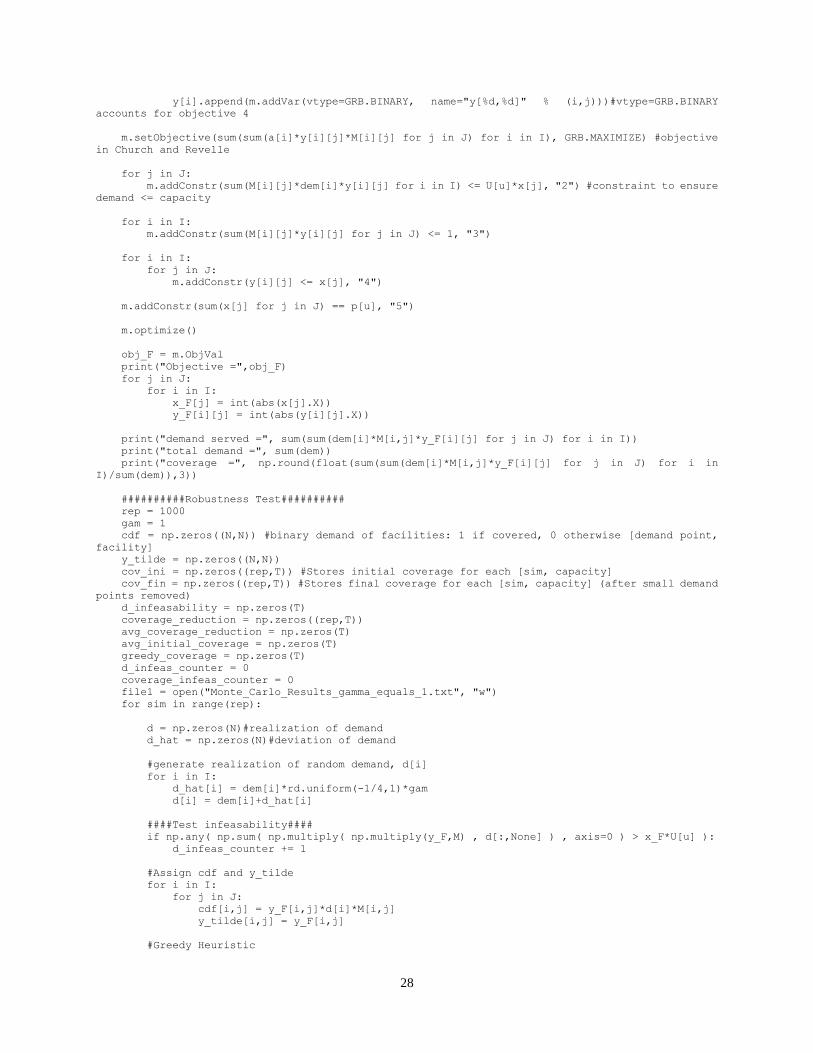
8.1 Python code for Maximum Coverage FLP
8.1.1 Deterministic
from gurobipy import *
import numpy as np
import random as rd
f = open("DataFileLarge.txt", "r")
for i in range(3):
line = f.readline()
data = line.split()
I = list(range(int(data[0])))
J = list(range(int(data[0])))
N = int(data[0])
P = int(data[1])
xy_coor = np.zeros((50,2))
dem = a = np.zeros(50)
for i in I:
line = f.readline()
data = line.split()
xy_coor[i,0] = int(data[1])
xy_coor[i,1] = int(data[2])
dem[i] = int(data[-1])
a[i] = int(data[-1])
T = 1 #number of capacities tested
U = np.ones(T)
L = np.zeros((N,N))
M = np.zeros((N,N))
s = np.zeros(T)#100000000 #coverage radius
p = np.zeros(T)
for u in range(T):
x_F = np.zeros(N)
y_F = np.zeros((N,N))
s[u] = 30#100000#(u+4)*5
#print("s =", s[u])
p[u] = P#(u+1)#P
print("p =", p[u])
for i in I:
for j in J:
L[i][j] = round((np.sqrt((xy_coor[i,0] - xy_coor[j,0])**2 + (xy_coor[i,1] -
xy_coor[j,1])**2)),2)
if L[i][j] <= s[u]:
M[i][j] = 1
else:
M[i][j] = 1000000
U[u] = sum(dem)/(0.8*p[u])#U[u]*70 + 10*u
print("Capacity =",U[u])
######DETERMINISTIC MODEL#######
m = Model("facility location")
m.setParam('OutputFlag',0)
x = [] #facility locations
for j in J:
x.append(m.addVar(vtype=GRB.BINARY, name="x[%d]" % j))#vtype=GRB.BINARY accounts for
objective 3
y = [] #Demand points
for i in I:
y.append([])
for j in J:
28
y[i].append(m.addVar(vtype=GRB.BINARY, name="y[%d,%d]" % (i,j)))#vtype=GRB.BINARY
accounts for objective 4
m.setObjective(sum(sum(a[i]*y[i][j]*M[i][j] for j in J) for i in I), GRB.MAXIMIZE) #objective
in Church and Revelle
for j in J:
m.addConstr(sum(M[i][j]*dem[i]*y[i][j] for i in I) <= U[u]*x[j], "2") #constraint to ensure
demand <= capacity
for i in I:
m.addConstr(sum(M[i][j]*y[i][j] for j in J) <= 1, "3")
for i in I:
for j in J:
m.addConstr(y[i][j] <= x[j], "4")
m.addConstr(sum(x[j] for j in J) == p[u], "5")
m.optimize()
obj_F = m.ObjVal
print("Objective =",obj_F)
for j in J:
for i in I:
x_F[j] = int(abs(x[j].X))
y_F[i][j] = int(abs(y[i][j].X))
print("demand served =", sum(sum(dem[i]*M[i,j]*y_F[i][j] for j in J) for i in I))
print("total demand =", sum(dem))
print("coverage =", np.round(float(sum(sum(dem[i]*M[i,j]*y_F[i][j] for j in J) for i in
I)/sum(dem)),3))
##########Robustness Test##########
rep = 1000
gam = 1
cdf = np.zeros((N,N)) #binary demand of facilities: 1 if covered, 0 otherwise [demand point,
facility]
y_tilde = np.zeros((N,N))
cov_ini = np.zeros((rep,T)) #Stores initial coverage for each [sim, capacity]
cov_fin = np.zeros((rep,T)) #Stores final coverage for each [sim, capacity] (after small demand
points removed)
d_infeasability = np.zeros(T)
coverage_reduction = np.zeros((rep,T))
avg_coverage_reduction = np.zeros(T)
avg_initial_coverage = np.zeros(T)
greedy_coverage = np.zeros(T)
d_infeas_counter = 0
coverage_infeas_counter = 0
file1 = open("Monte_Carlo_Results_gamma_equals_1.txt", "w")
for sim in range(rep):
d = np.zeros(N)#realization of demand
d_hat = np.zeros(N)#deviation of demand
#generate realization of random demand, d[i]
for i in I:
d_hat[i] = dem[i]*rd.uniform(-1/4,1)*gam
d[i] = dem[i]+d_hat[i]
####Test infeasability####
if np.any( np.sum( np.multiply( np.multiply(y_F,M) , d[:,None] ) , axis=0 ) > x_F*U[u] ):
d_infeas_counter += 1
#Assign cdf and y_tilde
for i in I:
for j in J:
cdf[i,j] = y_F[i,j]*d[i]*M[i,j]
y_tilde[i,j] = y_F[i,j]
#Greedy Heuristic
29
for j in J:
while sum(cdf[:,j]) > x_F[j]*U[u] and x_F[j] != 0:
minval = 10000000000
for i in cdf[:,j]:
if minval > i and i > 0:
minval = i
for i in I:
if minval == cdf[i,j]:
cdf[i,j] = 0
y_tilde[i,j] = 0
#To show greedy heuristic is effective
for j in J:
if sum(cdf[:,j] > x_F[j]*U[u]):
coverage_infeas_counter += 1
cov_fin[sim][u]= float(sum(sum(dem[i]*M[i,j]*y_tilde[i][j] for j in J) for i in
I)/sum(dem))
coverage_reduction[sim][u] = float(sum(sum(dem[i]*M[i,j]*y_F[i][j] for j in J) for i in
I)/sum(dem))-(float(sum(sum(dem[i]*M[i,j]*y_tilde[i][j] for j in J) for i in I)/sum(dem)))
d_infeasability[u] = d_infeas_counter/rep
coverage_infeasability = coverage_infeas_counter/rep
print("infeasability =", str(d_infeasability[u]))
print("greedy coverage =", np.round(float(sum(cov_fin[sim][u] for sim in range(rep))/rep),3))
print("coverage reduction =", np.round(float(sum(coverage_reduction[sim][u] for sim in
range(rep))/rep),3))
print("###########################")
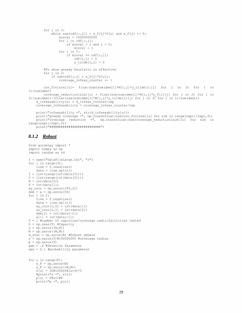
8.1.2 Robust
from gurobipy import *
import numpy as np
import random as rd
f = open("DataFileLarge.txt", "r")
for i in range(3):
line = f.readline()
data = line.split()
I = list(range(int(data[0])))
J = list(range(int(data[0])))
N = int(data[0])
P = int(data[1])
xy_coor = np.zeros((50,2))
dem = a = np.zeros(50)
for i in I:
line = f.readline()
data = line.split()
xy_coor[i,0] = int(data[1])
xy_coor[i,1] = int(data[2])
dem[i] = int(data[-1])
a[i] = int(data[-1])
T = 1 #number of capcities/coverage radii/facilities tested
U = np.ones(T) #Capacity
L = np.zeros((N,N))
M = np.zeros((N,N))
d_star = np.zeros(N) #Robust demand
s = np.zeros(T)#100000000 #coverage radius
p = np.zeros(T)
gam = .2 #Devation Parameter
eps = 0.1 #probability parameter
for u in range(T):
x_F = np.zeros(N)
y_F = np.zeros((N,N))
s[u] = 30#100000#(u+4)*5
#print("s =", s[u])
p[u] = P#u+1#P
print("p =", p[u])
30
for i in I:
for j in J:
L[i][j] = round((np.sqrt((xy_coor[i,0] - xy_coor[j,0])**2 + (xy_coor[i,1] -
xy_coor[j,1])**2)),2)
if L[i][j] <= s[u]:
M[i][j] = 1
else:
M[i][j] = 1000000
U[u] = sum(dem)/(0.8*p[u])#122.5#U[u]*70 + 10*u
print("Capacity =",U[u])
######ROBUST MODEL#######
for i in I:
d_star[i] = dem[i] + min(((1+gam)*dem[i])-dem[i],(((1-eps)/eps)*(dem[i]-((1-
gam)*dem[i]))),np.sqrt(((1-eps)/eps)*((((1+gam)*dem[i])-dem[i])*(dem[i]-(dem[i]*(1-gam))))))
m = Model("facility location")
m.setParam('OutputFlag',0)
x = [] #facility locations
for j in J:
x.append(m.addVar(vtype=GRB.BINARY, name="x[%d]" % j))#vtype=GRB.BINARY accounts for
objective 3
y = [] #Demand points
for i in I:
y.append([])
for j in J:
y[i].append(m.addVar(vtype=GRB.BINARY, name="y[%d,%d]" % (i,j)))#vtype=GRB.BINARY
accounts for objective 4
m.setObjective(sum(sum(a[i]*M[i,j]*y[i][j] for j in J) for i in I), GRB.MAXIMIZE) #objective
in Church and Revelle
for j in J:
m.addConstr(sum(M[i][j]*d_star[i]*y[i][j] for i in I) <= U[u]*x[j], "2") #constraint to
ensure demand <= capacity
for i in I:
m.addConstr(sum(M[i][j]*y[i][j] for j in J) <= 1, "3")
for i in I:
for j in J:
m.addConstr(y[i][j] <= x[j], "4")
m.addConstr(sum(x[j] for j in J) == p[u], "5")
m.optimize()
obj_F = m.ObjVal
print("Objective =", obj_F)
for j in J:
for i in I:
x_F[j] = int(abs(x[j].X))
y_F[i][j] = int(abs(y[i][j].X))
print("demand served = ", sum(sum(dem[i]*M[i,j]*y_F[i][j] for j in J) for i in I))
print("total demand = ", sum(dem))
print("coverage =", np.round(float(sum(sum(dem[i]*M[i,j]*y_F[i][j] for j in J) for i in
I)/sum(dem)),3))
##########Robustness Test##########
rep = 1000
cdf = np.zeros((N,N)) #binary demand of facilities: 1 if covered, 0 otherwise [demand point,
facility]
y_tilde = np.zeros((N,N))
cov_ini = np.zeros((rep,T)) #Stores initial coverage for each [sim, capacity]
31
cov_fin = np.zeros((rep,T)) #Stores final coverage for each [sim, capacity] (after small demand
points removed)
d_infeasability = np.zeros(T)
coverage_reduction = np.zeros((rep,T))
avg_coverage_reduction = np.zeros(T)
avg_initial_coverage = np.zeros(T)
greedy_coverage = np.zeros(T)
d_infeas_counter = 0
coverage_infeas_counter = 0
file1 = open("Robust_Monte_Carlo_Results_gamma_equals_1.txt", "w")
for sim in range(rep):
d = np.zeros(N)#realization of demand
d_hat = np.zeros(N)#deviation of demand
#generate realization of random demand, d[i]
for i in I:
d_hat[i] = dem[i]*rd.uniform(-1/4,1)*gam
d[i] = dem[i]+d_hat[i]
####Test infeasability####
if np.any( np.sum( np.multiply( np.multiply(y_F,M) , d[:,None] ) , axis=0 ) > x_F*U[u] ):
d_infeas_counter += 1
#Assign cdf and y_tilde
for i in I:
for j in J:
cdf[i,j] = y_F[i,j]*d[i]
y_tilde[i,j] = y_F[i,j]
#Greedy Heuristic
for j in J:
while sum(cdf[:,j]) > x_F[j]*U[u] and x_F[j] != 0:
minval = 10000000
for i in cdf[:,j]:
if minval > i and i > 0:
minval = i
for i in I:
if minval == cdf[i,j]:
cdf[i,j] = 0
y_tilde[i,j] = 0
#To show greedy Heuristic is effective
for j in J:
if sum(cdf[:,j] > x_F[j]*U[u]):
coverage_infeas_counter += 1
cov_fin[sim][u]= float(sum(sum(dem[i]*M[i,j]*y_tilde[i][j] for j in J) for i in
I)/sum(dem))
coverage_reduction[sim][u] = float(sum(sum(dem[i]*M[i,j]*y_F[i][j] for j in J) for i in
I)/sum(dem))-(float(sum(sum(dem[i]*M[i,j]*y_tilde[i][j] for j in J) for i in I)/sum(dem)))
d_infeasability[u] = d_infeas_counter/rep
coverage_infeasability = coverage_infeas_counter/rep
print("infeasability =", str(d_infeasability[u]))
print("greedy coverage =", np.round(float(sum(cov_fin[sim][u] for sim in range(rep))/rep),3))
print("coverage reduction =", np.round(float(sum(coverage_reduction[sim][u] for sim in
range(rep))/rep),3))
print("###########################")
8.2 Python code for Minimum Cost FLP
8.2.1 Deterministic
from gurobipy import *
import numpy as np
import random as rd
# 1040444.375
32
# J.E.Beasley "An algorithm for solving
# large capacitated warehouse location problems" European
# Journal of Operational Research 33 (1988) 314-325.
f = open("cap41.txt", "r")
line = f.readline()
data = line.split()
num_loc = int(data[0])
num_cust = int(data[1])
I = list(range(num_cust))
J = list(range(num_loc))
u = np.zeros(num_loc)
fc = np.zeros(num_loc)
d = np.zeros(num_cust)
c = np.zeros((num_cust,num_loc))
gam = 0.35
rep = 1000
penalty = 0
for j in J:
line = f.readline()
data = line.split()
u[j] = int(data[0])
fc[j] = float(data[1])
for i in I:
line = f.readline()
d[i] = (int(line))
line = f.readline()
data = line.split()
for j in J:
c[i,j] = (float(data[j]))
f.close()
m = Model("facility location")
y = []
for j in J:
y.append(m.addVar(vtype=GRB.BINARY, name="open[%d]" % i))
x = []
for i in I:
x.append([])
for j in J:
x[i].append(m.addVar(lb = 0, ub = 1, name="trans[%d,%d]" % (i, j)))
m.setObjective(quicksum(fc[j]*y[j] for j in J) + quicksum(c[i][j]*x[i][j] for j in J for i in I),
GRB.MINIMIZE)
for i in I:
m.addConstr(sum(x[i][j] for j in J) == 1, "Demand[%d]" % i)
for j in J:
m.addConstr(sum(d[i]*x[i][j] for i in I) <= u[j]*y[j], "Capacity[%d]" % j)
for i in I:
for j in J:
m.addConstr(x[i][j] <= y[j], "Feasibility[%d][%d]" %(i,j))
m.optimize()
'''
# Print solution
f = open("output.txt", "w")
f.write('\nTOTAL COSTS: %g' % m.objVal)
f.write('\nSOLUTION:')
for j in J:
if y[j].x > 0.99:
f.write('\nPlant %s open' % j)
for i in I:
if x[i][j].x > 0:
f.write('\n Transport %g units to customer %s' % (x[i][j].x, i))
else:
33
f.write('\nPlant %s closed!' % j)
f.close()
'''
import networkx as nx
import matplotlib.pyplot as plt
plt.figure(figsize=(10,10))
cust_x = [rd.uniform(1,10) for i in I]
cust_y = [rd.uniform(0,10) for i in I]
fac_x = [rd.uniform(0,1) for j in J]
fac_y = [rd.uniform(0,10) for j in J]
connection = [(i,50+j) for i in I for j in J if x[i][j].x > 0]
fac_nodes = [j for j in J if y[j].x > 0]
cust_nodes = [i for i in I]
G = nx.Graph()
G.add_edges_from(connection)
for i in I:
G.add_node(i, pos = (cust_x[i], cust_y[i]))
print("Number of nodes: ", G.number_of_nodes())
for i in J:
if y[i].x > 0:
G.add_node(50+i, pos = (fac_x[i],fac_y[i]))
print("Number of nodes: ", G.number_of_nodes())
#node_col = nx.get_node_attributes(G,'color')
node_col = ['blue' if node < len(I) else 'red' for node in G.nodes()]
node_pos=nx.get_node_attributes(G,'pos')
#nx.draw_networkx(G,node_pos, node_color = node_col)
nx.draw(G,node_pos, node_color = node_col)
#nx.draw_networkx_edges(G, node_pos)
#plt.axis('off')
# Show the plot
plt.show()
obj_F = m.ObjVal
y_F = np.zeros(num_loc)
x_F = np.zeros((num_cust,num_loc))
for j in J:
for i in I:
y_F[j] = int(abs(y[j].X))
x_F[i][j] = (abs(x[i][j].X))
cdf = np.zeros((num_cust,num_loc))
cov_ini = np.zeros(rep)
cov_fin = np.zeros(rep)
cost_ini = np.zeros(rep)
cost_fin = np.zeros(rep)
change_x = np.zeros(rep)
x_fin = np.zeros((num_cust,num_loc)) #x value after removing infeasible points
####Monte Carlo Simulation#####
infeas_counter = 0
coverage_infeas_counter = 0
file1 = open("Monte_Carlo_Results_gamma_equals_1.txt", "w")
for sim in range(rep):
d_hat = np.zeros(num_cust)
d_rd = np.zeros(num_cust)
#generate realization of random demand, d[i]
34
for i in I:
d_hat[i] = d[i]*rd.uniform(-1,1)*gam
d_rd[i] = d[i]+d_hat[i]
####Test infeasability####
if np.any( np.sum( np.multiply(d_rd[:,None],x_F) ) > y_F*u[u] , axis=0):
infeas_counter += 1
#Calculate cost initially
cost_ini[sim] = sum(fc[j]*y_F[j] for j in J) + sum(sum(c[i,j]*x_F[i,j] for j in J) for i in I)
####Test Coverage####
for i in I:
for j in range(int(sum(y_F))):
cdf[i,j] = x_F[i,j]*d_rd[i]
cov_ini[sim] = np.sum(cdf)
for i in I:
for j in J:
x_fin[i,j] = x_F[i,j]
#Greedy Heuristic
for j in J:
while sum(cdf[:,j]) > u[j]:
minval = 10000000000
for i in cdf[:,j]:
if minval > i and i > 0:
minval = i
for i in I:
if minval == cdf[i,j]:
cdf[i,j] = 0
x_fin[i,j] = 0
change_x[sim] = np.sum(x_F) - np.sum(x_fin)
cov_fin[sim] = np.sum(cdf)
cost_fin[sim] = sum(fc[j]*y_F[j] for j in J) + sum(sum(c[i,j]*x_fin[i,j] for j in J) for i in
I) + sum(sum(penalty*d[i]*(x_F[i,j]-x_fin[i,j]) for i in I) for j in J)
print("infeasibility = ", infeas_counter/rep)
print("initial coverage = ", sum(cov_ini)/rep)
print("final coverage =", sum(cov_fin)/rep)
print("initial cost = ", sum(cost_ini)/rep)
print("final cost = ", sum(cost_fin)/rep)
print("change in cost = ", (sum(cost_ini)/rep)-(sum(cost_fin)/rep))
8.2.2 Robust
from gurobipy import *
import numpy as np
import random as rd
# 1040444.375
# J.E.Beasley "An algorithm for solving
# large capacitated warehouse location problems" European
# Journal of Operational Research 33 (1988) 314-325.
f = open("cap41.txt", "r")
line = f.readline()
data = line.split()
num_loc = int(data[0])
num_cust = int(data[1])
I = list(range(num_cust))
J = list(range(num_loc))
u = np.zeros(num_loc) #capcity
fc = np.zeros(num_loc) #fixed cost
d = np.zeros(num_cust) #demand
d_star = np.zeros(num_cust) #robust demand
c = np.zeros((num_cust,num_loc)) #cost of serving customer
gamma = 0.2
epsilon = 0.05
35
rep = 1000
for j in J:
line = f.readline()
data = line.split()
u[j] = int(data[0])
fc[j] = float(data[1])
for i in I:
line = f.readline()
d[i] = (int(line))
line = f.readline()
data = line.split()
for j in J:
c[i,j] = (float(data[j]))
f.close()
for i in I:
d_star[i] = d[i] + min(((1+gamma)*d[i])-d[i],((1-epsilon)/epsilon)*(d[i]-(d[i]*(1-
gamma))),(np.sqrt(((1-epsilon)/epsilon)*((((1+gamma)*d[i])-d[i])*(d[i]-(d[i]*(1-gamma)))))))
m = Model("facility location")
y = []
for j in J:
y.append(m.addVar(vtype=GRB.BINARY, obj=fc[j], name="open[%d]" % i))
x = []
for i in I:
x.append([])
for j in J:
x[i].append(m.addVar(obj=c[i][j], lb = 0, ub = 1, name="trans[%d,%d]" % (i, j)))
# Other ways to add variables
#y = m.addVars(num_loc, vtype=GRB.BINARY, obj=fc, name="open")
#x = m.addVars(num_cust, num_loc, obj=c, lb = 0, ub = 1, name="trans")
#x = []
#for i in cust:
# for j in loc:
# x[i][j] = m.addVar(obj=c[i][j], lb = 0, ub = 1, name="trans[%d,%d]" % (i, j))
m.modelSense = GRB.MINIMIZE
for i in I:
m.addConstr(sum(x[i][j] for j in J) == 1, "Demand[%d]" % i)
for j in J:
m.addConstr(sum(d_star[i]*x[i][j] for i in I) <= u[j]*y[j], "Capacity[%d]" % j)
for i in I:
for j in J:
m.addConstr(x[i][j] <= y[j], "Feasibility[%d][%d]" %(i,j))
m.optimize()
'''
# Print solution
f = open("robust_output.txt", "w")
f.write('\nTOTAL COSTS: %g' % m.objVal)
f.write('\nSOLUTION:')
for j in J:
if y[j].x > 0.99:
f.write('\nPlant %s open' % j)
for i in I:
if x[i][j].x > 0:
f.write('\n Transport %g units to customer %s' % (x[i][j].x, i))
else:
f.write('\nPlant %s closed!' % j)
f.close()
'''
import networkx as nx
import matplotlib.pyplot as plt
36
plt.figure(figsize=(10,10))
cust_x = [rd.uniform(1,10) for i in I]
cust_y = [rd.uniform(0,10) for i in I]
fac_x = [rd.uniform(0,1) for j in J]
fac_y = [rd.uniform(0,10) for j in J]
connection = [(i,50+j) for i in I for j in J if x[i][j].x > 0]
fac_nodes = [j for j in J if y[j].x > 0]
cust_nodes = [i for i in I]
G = nx.Graph()
G.add_edges_from(connection)
for i in I:
G.add_node(i, pos = (cust_x[i], cust_y[i]))
print("Number of nodes: ", G.number_of_nodes())
for i in J:
if y[i].x > 0:
G.add_node(50+i, pos = (fac_x[i],fac_y[i]))
print("Number of nodes: ", G.number_of_nodes())
#node_col = nx.get_node_attributes(G,'color')
node_col = ['blue' if node < len(I) else 'red' for node in G.nodes()]
node_pos=nx.get_node_attributes(G,'pos')
#nx.draw_networkx(G,node_pos, node_color = node_col)
nx.draw(G,node_pos, node_color = node_col)
#nx.draw_networkx_edges(G, node_pos)
#plt.axis('off')
# Show the plot
plt.show()
obj_F = m.ObjVal
y_F = np.zeros(num_loc)
x_F = np.zeros((num_cust,num_loc))
for j in J:
for i in I:
y_F[j] = int(abs(y[j].X))
x_F[i][j] = (abs(x[i][j].X))
cdf = np.zeros((num_cust,num_loc))
cov_ini = np.zeros(rep)
cov_fin = np.zeros(rep)
cost_ini = np.zeros(rep)
cost_fin = np.zeros(rep)
change_x = np.zeros(rep)
x_fin = np.zeros((num_cust,num_loc)) #x value after removing infeasible points
####Monte Carlo Simulation#####
infeas_counter = 0
coverage_infeas_counter = 0
file1 = open("Monte_Carlo_Results_gamma_equals_1.txt", "w")
for sim in range(rep):
d_hat = np.zeros(num_cust)
d_rd = np.zeros(num_cust)
#generate realization of random demand, d[i]
for i in I:
d_hat[i] = d[i]*rd.uniform(-0.5,1)*gamma
d_rd[i] = d[i]+d_hat[i]
####Test infeasability####
37
if np.any( np.sum( np.multiply(d_rd[:,None],x_F) ) > y_F*u[u] , axis=0):
infeas_counter += 1
#Calculate cost initially
cost_ini[sim] = sum(fc[j]*y_F[j] for j in J) + sum(sum(c[i,j]*x_F[i,j] for j in J) for i in I)
####Test Coverage####
for i in I:
for j in J:
cdf[i,j] = x_F[i,j]*d_rd[i]
cov_ini[sim] = np.sum(cdf)
for i in I:
for j in J:
x_fin[i,j] = x_F[i,j]
#Greedy Heuristic
for j in J:
while sum(cdf[:,j]) > u[j]:
minval = 10000000000
for i in cdf[:,j]:
if minval > i and i > 0:
minval = i
for i in I:
if minval == cdf[i,j]:
cdf[i,j] = 0
x_fin[i,j] = 0
change_x[sim] = np.sum(x_F) - np.sum(x_fin)
cov_fin[sim] = np.sum(cdf)
cost_fin[sim] = sum(fc[j]*y_F[j] for j in J) + sum(sum(c[i,j]*x_fin[i,j] for j in J) for i in
I)
print("infeasibility = ", infeas_counter/rep)
print("initial coverage = ", sum(cov_ini)/rep)
print("final coverage =", sum(cov_fin)/rep)
print("initial cost = ", sum(cost_ini)/rep)
print("final cost = ", sum(cost_fin)/rep)
print("change in cost = ", (sum(cost_ini)/rep)-(sum(cost_fin)/rep))
print("change in x = ", sum(change_x)/rep)