DISTRIBUTIONAL NATIONAL ACCOUNTS:METHODS AND ESTIMATES FOR THE UNITED

STATES∗

Thomas PikettyEmmanuel SaezGabriel Zucman

September 25, 2017

Abstract

This paper combines tax, survey, and national accounts data to estimate the distributionof national income in the United States since 1913. Our distributional national accountscapture 100% of national income, allowing us to compute growth rates for each quantile ofthe income distribution consistent with macroeconomic growth. We estimate the distribu-tion of both pre-tax and post-tax income, making it possible to provide a comprehensiveview of how government redistribution affects inequality. Average pre-tax real nationalincome per adult has increased 60% since 1980, but we find that it has stagnated for thebottom 50% of the distribution at about $16,000 a year. The pre-tax income of the middleclass—adults between the median and the 90th percentile—has grown 40% since 1980,faster than what tax and survey data suggest, due in particular to the rise of tax-exemptfringe benefits. Income has boomed at the top. The upsurge of top incomes was first alabor income phenomenon but has mostly been a capital income phenomenon since 2000.The government has offset only a small fraction of the increase in inequality. The reduc-tion of the gender gap in earnings has mitigated the increase in inequality among adults,but the share of women falls steeply as one moves up the labor income distribution, andis only 11% in the top 0.1% in 2014. JEL Codes: E01, H2, H5, J3.

∗Thomas Piketty: piketty@psemail.eu; Emmanuel Saez: saez@econ.berkeley.edu; Gabriel Zucman: zuc-man@berkeley.edu. An online appendix and a set of appendix tables and figures supplementing this articleare available online at http://gabriel-zucman.eu/usdina. We thank Facundo Alvaredo, Tony Atkinson,Gerald Auten, Lucas Chancel, Patrick Driessen, Oded Galor, David Johnson, Arthur Kennickell, Nora Lustig,Jean-Laurent Rosenthal, John Sabelhaus, David Splinter, and numerous seminar and conference participantsfor helpful discussions and comments. Antoine Arnoud, Kaveh Danesh, Sam Karlin, Juliana Londono-Velez,Carl McPherson provided outstanding research assistance. We acknowledge financial support from the Centerfor Equitable Growth at UC Berkeley, the Institute for New Economic Thinking, the Laura and John Arnoldfoundation, NSF grants SES-1156240 and SES-1559014, the Russell Sage foundation, the Sandler foundation,and the European Research Council under the European Union’s Seventh Framework Programme, ERC GrantAgreement No. 340831.

I. Introduction

Income inequality has increased in many developed countries over the last several decades.

This trend has attracted considerable interest among academics, policy-makers, and the general

public. In recent years, following up on Kuznets’ (1953) pioneering attempt, a number of authors

have used administrative tax records to construct long-run series of top income shares (Alvaredo

et al., 2011-2017). Yet despite this endeavor, we still face three important limitations when

measuring income inequality. First and most important, there is a large gap between national

accounts—which focus on macro totals and growth—and inequality studies—which focus on

distributions using survey and tax data, usually without trying to be fully consistent with

macro totals. This gap makes it hard to address questions such as: What fraction of economic

growth accrues to the bottom 50%, the middle 40%, and the top 10% of the distribution? How

much of the rise in income inequality owes to changes in the share of labor and capital in national

income, and how much to changes in the dispersion of labor earnings, capital ownership, and

returns to capital? Second, about a third of U.S. national income is redistributed through taxes,

transfers, and public spending on goods and services such as education, police, and defense. Yet

we do not have a comprehensive measure of how the distribution of pre-tax income differs from

the distribution of post-tax income, making it hard to assess how government redistribution

affects inequality. Third, existing income inequality statistics use the tax unit or the household

as unit of observation, adding up the income of men and women. As a result, we do not have

a clear view of how long-run trends in income concentration are shaped by the major changes

in women labor force participation—and gender inequality generally—that have occurred over

the last century.

This paper attempts to compute inequality statistics for the United States that overcome the

limits of existing series by creating distributional national accounts. We combine tax, survey,

and national accounts data to build new series on the distribution of national income since

1913. In contrast to previous attempts that capture less than 60% of US national income—

such as Census bureau estimates (US Census Bureau 2016) and top income shares (Piketty

and Saez, 2003)—our estimates capture 100% of the national income recorded in the national

accounts. This enables us to provide decompositions of growth by income groups consistent

with macroeconomic growth. We compute the distribution of both pre-tax and post-tax income.

Post-tax series deduct all taxes and add back all transfers and public spending, so that both

pre-tax and post-tax incomes add up to national income. This allows us to provide the first

comprehensive view of how government redistribution affects inequality. Our benchmark series

1

uses the adult individual as the unit of observation and splits income equally among spouses.

We also report series in which each spouse is assigned her or his own labor income, enabling us

to study how long-run changes in gender inequality shape the distribution of income.

Distributional national accounts provide information on the dynamic of income across the

entire spectrum—from the bottom decile to the top 0.001%—that, we believe, is more accurate

than existing inequality data. Our estimates capture employee fringe benefits, a growing source

of income for the middle-class that is overlooked by both Census bureau estimates and tax

data. They capture all capital income, which is large—about 30% of total national income—

and concentrated, yet is very imperfectly covered by surveys—due to small sample and top

coding issues—and by tax data—as a large fraction of capital income goes to pension funds and

is retained in corporations. They make it possible to produce long-run inequality statistics that

control for socio-demographic changes—such as the rise in the fraction of retired individuals

and the decline in household size—contrary to the currently available tax-based series.

Methodologically, our contribution is to construct micro-files of pre-tax and post-tax income

consistent with macro aggregates. These micro-files contain all the variables of the national

accounts and synthetic adult individual observations that we obtain by statistically matching

tax and survey data and making explicit assumptions about the distribution of income categories

for which there is no directly available source of information. By construction, the totals in

these micro-files add up to the national accounts totals, while the distributions are consistent

with those seen in tax and survey data. These files can be used to compute a wide array of

distributional statistics—labor and capital income earned, taxes paid, transfers received, wealth

owned, etc.—by age groups, gender, and marital status. Our objective, in the years ahead, is

to construct similar micro-files in as many countries as possible to better compare inequality

across countries.1 Just like we use GDP or national income to compare the macroeconomic

performances of countries today, so could distributional national accounts be used to compare

inequality across countries tomorrow.

We stress at the outset that there are numerous data issues involved in distributing national

income, discussed in the text and the online appendix.2 First, we take the national accounts

as a given starting point, although we are well aware that the national accounts themselves are

imperfect (e.g., Zucman 2013). They are, however, the most reasonable starting point, because

they aggregate all the available information from surveys, tax data, corporate income state-

1All the results will be made available on the World Wealth and Income Database (WID.world) website:http://wid.world/.

2The online appendix and data files are available at http://gabriel-zucman.eu/usdina.

2

ments and balance sheets, etc., in an standardized, internationally-agreed-upon and regularly

improved upon accounting framework. Second, imputing all national income, taxes, transfers,

and public goods spending requires making assumptions on a number of complex issues, such as

the economic incidence of taxes and who benefits from government spending. Our goal is not to

provide definitive answers to these questions, but rather to be comprehensive, consistent, and

explicit about what assumptions we are making and why. We view our paper as attempting to

construct prototype distributional national accounts, a prototype that could be improved upon

as more data become available, new knowledge emerges on who pays taxes and benefits from

government spending, and refined estimation techniques are developed—just as today’s national

accounts are regularly improved. Third, our estimates of incomes at the top of the distribution

are based on tax data, hence disregard tax evasion. Because top marginal tax rates, tax evasion

technologies, and tax enforcement strategies have changed a lot over time, tax data may paint

a biased picture of income concentration at the very top.3

The analysis of our US distributional national accounts yields a number of striking findings.

First, our data show a sharp divergence in the growth experienced by the bottom 50% versus

the rest of the economy. The average pre-tax income of the bottom 50% of adults has stagnated

at about $16,000 per adult (in constant 2014 dollars, using the national income deflator) since

1980, while average national income per adult has grown by 60% to $64,500 in 2014. As a

result, the bottom 50% income share has collapsed from about 20% in 1980 to 12% in 2014. In

the meantime, the average pre-tax income of top 1% adults rose from $420,000 to about $1.3

million, and their income share increased from about 12% in the early 1980s to 20% in 2014.

The two groups have essentially switched their income shares, with 8 points of national income

transferred from the bottom 50% to the top 1%. The top 1% income share is now almost twice

as large as the bottom 50% share, a group that is by definition 50 times more numerous. In

1980, top 1% adults earned on average 27 times more than bottom 50% adults before tax, while

they earn 81 times more today.

Second, government redistribution has offset only a small fraction of the increase in pre-tax

inequality. Even after taxes and transfers, there has been close to zero growth for working-age

adults in the bottom 50% of the distribution since 1980. The aggregate flow of individualized

government transfers has increased, but these transfers are largely targeted to the elderly and

3Using random audits and random leaks from offshore financial institutions, Alstadsæter, Johannesen andZucman (2017) find that the top 0.01% richest Scandinavians evade about 25% of their taxes. Alstadsæter,Johannesen and Zucman (2017b) investigate the implications of top-end tax evasion for wealth distributions ina sample of 10 countries including the United States. In future work we plan to include estimates of tax evasioninto our distributional national accounts.

3

the middle-class (individuals above the median and below the 90th percentile). Transfers that

go to the bottom 50% of earners have not been large enough to lift their incomes significantly.

Third, we find that the upsurge of top incomes has mostly been a capital-driven phenomenon

since the late 1990s. There is a widespread view that rising income inequality mostly owes to

booming wages at the top end (Piketty and Saez, 2003). Our results confirm that this view is

correct from the 1970s to the 1990s. But in contrast to earlier decades, the increase in income

concentration over the last fifteen years owes to a boom in the income from equity and bonds

at the top. Top earners became younger in the 1980s and 1990s but have been growing older

since then.

Fourth, the reduction in the gender gap has mitigated the increase in inequality among

adults since the late 1960s, but the United States is still characterized by a spectacular glass

ceiling. When we allocate labor incomes to individual earners (instead of splitting it equally

within couples, as we do in our benchmark series), the rise in inequality is less dramatic, thanks

to the rise of female labor market participation. Men aged 20-64 earned on average 3.7 times

more labor income than women aged 20-64 in the early 1960s, while they earn 1.7 times more

today. Until the early 1980s, the top 10%, top 1%, and top 0.1% of the labor income distribution

were less than 10% women. Since then, this share has increased, but the increase is smaller the

higher one moves up in the distribution. As of 2014, women make only about 16% of the top

1% labor income earners, and 11% of the top 0.1%.

The paper is organized as follows. Section II. relates our work to the existing literature.

Section III. lays out our methodology. In Section IV., we present our results on the distribution

of pre-tax and post-tax national income, and we provide decompositions of growth by income

groups consistent with macroeconomic growth. Section V. analyzes the role of changes in gender

inequality, capital vs. labor factor shares, and taxes and transfers for the dynamic of US income

inequality. We conclude in Section VI.

II. Previous Attempts at Introducing Distributional

Measures in the National Accounts

There is a long tradition of research attempting to introduce distributional measures in the

national accounts. The first national accounts in history—the famous social tables of King

produced in the late 17th century—were in fact distributional national accounts, showing the

distribution of England’s income, consumption, and saving across 26 social classes—from tem-

poral lords and baronets down to vagrants—in the year 1688 (see Barnett, 1936). In the United

4

States, Kuznets was interested in both national income and its distribution and made path-

breaking advances on both fronts (Kuznets 1941, 1953).4 His innovation was estimating top

income shares by combining tabulations of federal income tax returns—from which he derived

the income of top earners using Pareto extrapolations—and newly constructed national accounts

series—that he used to compute the total income denominator. Kuznets, however, did not fully

integrate the two approaches: his inequality series capture taxable income only and miss all

tax-exempt capital and labor income. The top income shares later computed by Piketty (2001,

2003), Piketty and Saez (2003), Atkinson (2005) and Alvaredo et al. (2011-2017) extended

Kuznets’ methodology to more countries and years but did not address this shortcoming.

Introducing distributional measures in the national accounts has received renewed interest in

recent years. In 2009, a report from the Commission on the Measurement of Economic Perfor-

mance and Social Progress emphasized the importance of including distributional measures such

as household income quintiles in the System of National Accounts (Stiglitz, Sen and Fitoussi,

2009). In response to this report, on OECD Expert Group on the Distribution of National

Accounts was created. A number of countries, such as Australia, have introduced distributional

statistics in their national accounts (Australian Bureau of Statistic, 2013) while others are in

the process of doing so. Furlong (2014), Fixler and Johnson (2014), McCully (2014), and Fixler

et al. (2015) describe the ongoing U.S. effort, which focuses on scaling up income from the

Current Population Survey to match personal income.5

There are two main methodological differences between our paper and the work currently

conducted by statistical agencies. First, we start with tax data—rather than surveys—that we

supplement with surveys to capture forms of income that are not visible in tax returns, such

as tax-exempt transfers. The use of tax data is critical to capture the top of the distribution,

which cannot be studied properly with surveys because of top-coding, insufficient over-sampling

of the top, sampling errors, or non-sampling errors.6 Second, we are primarily interested in

4Earlier attempts include King (1915, 1927, 1930).5Using tax data, Auten and Splinter (2017) have recently produced US top income share series since 1960

by broadening the fiscal income definition. Instead of attempting to systematically match national income aswe do, they add components to fiscal income. Their estimates capture about 75% of national income in recentyears. They find much more modest increases in the top 1% income share for reasons we discuss in detail in theonline appendix section C. Their work is still in progress and we will update our online appendix accordingly.Armour et al. (2014) also construct distributions which go beyond the market income reported on tax returns.

6Some studies have attempted to measure the world distribution of income by also combining national ac-counts with survey data but without using individual tax data (e.g., Sala-i-Martin, 2006; Lakner and Milanovic,2013). Tax data are critical to capture the top and to reconcile survey income with macro income. Part ofgap between surveys and national accounts is also due to mis-measurement in national accounts, especially indeveloping countries where national accounts are not as well developed as in advanced economies (see Deaton,2005) for a thorough discussion).

5

the distribution of total national income rather than household or personal income. National

income is in our view a more meaningful starting point, because it is internationally comparable,

it is the aggregate used to compute macroeconomic growth, and it is comprehensive, including

all forms of income that eventually accrue to individuals.7 While we focus on national income,

our micro-files can be used to study a wide range of income concepts, including the household

or personal income concepts more traditionally analyzed.

Little work has contrasted the distribution of pre-tax income with that of post-tax income.

Top income share studies only deal with pre-tax income, as many forms of transfers are tax-

exempt. Official income statistics from the Census Bureau focus on pre-tax income and include

only some government transfers (US Census Bureau 2016).8 Congressional Budget Office (2016)

estimates compute both pre-tax and post-tax inequality measures, but they include only Federal

taxes—disregarding state and local taxes, which amount to around 10% of national income—and

do not try to incorporate government consumption, which is large too—about 18% of national

income. By contrast, we attempt to allocate all taxes (including state and local taxes) and all

forms of government spending in order to provide a comprehensive view of how government

redistribution affects inequality.

III. Methodology to Distribute US National Income

In this section, we outline the main concepts and methodology we use to distribute US

national income. All the data sources and computer code we use are described in Online

Appendix A; here we focus on the main conceptual issues.9

III.A. The Income Concept We Use: National Income

We are interested in the distribution of total national income. We follow the official defini-

tion of national income codified in the latest System of National Accounts,10 as we do for all

other national accounts concepts used in this paper. National income is GDP minus capital

7Personal income is a concept that is specific to the U.S. National Income and Product Accounts (NIPA).It is an ambiguous concept (neither pre-tax, nor post-tax), as it does not deduct taxes but adds back cashgovernment transfers. The System of National Accounts (United Nations, 2009) does not use personal income.

8In our view, not deducting taxes but counting (some) transfers is not conceptually meaningful, but it parallelsthe definition of personal income in the US national accounts.

9A discussion of the general issues involved in creating distributional national accounts and general guidelinesare presented in Alvaredo et al. (2016). These guidelines are not specific to the United States but they arebased on the lessons learned from constructing the US distributional national accounts presented here, and fromsimilar on-going projects in other countries.

10See United Nations (2009) for a thorough presentation of the System of National Accounts.

6

depreciation plus net income received from abroad. Although macroeconomists, the press, and

the general public often focus on GDP, national income is a more meaningful starting point

for two reasons. First, capital depreciation is not economic income: it does not allow one to

consume or accumulate wealth. Allocating depreciation to individuals would artificially inflate

the economic income of capital owners. Second, including foreign income is important, because

foreign dividends and interest are sizable for top earners.11 In moving away from GDP and

toward national income, we follow one of the recommendations made by the Stiglitz, Sen and

Fitoussi (2009) commission and also return to the pre-World War II focus on national income

(King 1930, Kuznets, 1941).

The national income of the United States is the sum of all the labor income—the flow return

to human capital—and capital income—the flow return to non-human capital—that accrues

to U.S. resident individuals. Some parts of national income never show up on any person’s

bank account, but it is not a reason to ignore them. Two prominent examples are the imputed

rents of homeowners and taxes. First, there is an economic return to owning a house, whether

the house is rented or not; national income therefore includes both monetary rents—for houses

rented out—and imputed rents—for owner-occupiers. Second, some income is immediately paid

to the government in the form of payroll or corporate taxes. But these taxes are part of the flow

return to capital and labor and as such accrue to the owners of the factors of production. The

same is true for sales and excise taxes. Out of their sales proceeds at market prices (including

sales taxes), producers pay workers labor income and owners capital income but must also pay

sales and excise taxes to the government. Hence, sales and excise taxes are part of national

income even if they are not explicitly part of employee compensation or profits. Who exactly

earns the fraction of national income paid in the form of corporate, payroll, and sales taxes is

a tax incidence question to which we return in Section III.C. below. Although national income

includes all the flow return to the factors of production, it does not include the change in the

price of these factors; i.e., it excludes the capital gains caused by pure asset price changes.12

11National income also includes the sizable flow of undistributed profits reinvested in foreign companies thatare more than 10% U.S.-owned (hence are classified as U.S. direct investments abroad). It does not, however,include undistributed profits reinvested in foreign companies in which the U.S. owns a share of less than 10%(classified as portfolio investments). Symmetrically, national income deducts all the primary income paid by theU.S. to non-residents, including the undistributed profits reinvested in U.S. companies that are more than 10%foreign-owned.

12In the long-run, a large fraction of capital gains arises from the fact that corporations retain part of theirearnings, which leads to share price appreciation. Since retained earnings are part of national income, thesecapital gains are in effect included in our series on an accrual basis. In the short run, however, most capital gainsare pure asset price effects. These short-term capital gains are excluded from national income and from ourseries. Our micro-data also provide estimates of individual wealth by broad asset class as in Saez and Zucman(2016) that can be used to study capital gains due to price effects.

7

National income is larger and has been growing faster than the other income concepts tradi-

tionally used to study inequality. Figure I provides a reconciliation between national income—as

recorded in the national accounts—and the fiscal income reported by individual taxpayers to the

IRS, for labor and capital income separately.13 About 70% of national income is labor income

and 30% is capital income. Although most of national labor income is reported on tax returns

today, the gap between taxable labor income and national labor income has been growing over

the last several decades. Untaxed labor income includes tax-exempt fringe benefits, employer

payroll taxes, the labor income of non filers (large before the early 1940s) and unreported labor

income due to tax evasion. The fraction of labor income which is taxable has declined from 80%-

85% in the post-World War II decades to just under 70% in 2014, due to the rise of employee

fringe benefits. As for capital, only a third of total capital income is reported on tax returns.

In addition to the imputed rents of homeowners and various taxes, untaxed capital income in-

cludes the dividends and interest paid to tax-exempt pension accounts and corporate retained

earnings. The low ratio of taxable to total capital income is not a new phenomenon—there is no

trend in this ratio over time. However, when taking into account both labor and capital income,

the fraction of national income that is reported in individual income tax data has declined from

70% in the late 1970s to about 60% today. This implies that tax data under-estimate both

the levels and growth rates of U.S. incomes.14 They particularly under-estimate growth for the

middle-class, as we shall see.

III.B. Pre-tax Income and Post-tax Income

At the individual level, income differs whether it is observed before or after the operation of

the pension system and government redistribution. We therefore define three income concepts

that all add up to national income: pre-tax factor income, pre-tax national income, and post-tax

national income. The key difference between pre-tax factor income and pre-tax national income

is the treatment of pensions, which are counted on a contribution basis for pre-tax factor income

and on a distribution basis for pre-tax national income. Post-tax national income deducts all

taxes and adds back all public spending, including public goods consumption. By construction,

13A number of studies have tried to reconcile totals from the national accounts and totals from householdsurveys or tax data; see, e.g., Fesseau, Wolff and Mattonetti (2012) and Fesseau and Mattonetti (2013). Suchcomparisons have long been conducted at national levels (for example, Atkinson and Micklewright, 1983, forthe UK) and there have been earlier cross country comparisons (for example in the OECD report by Atkinson,Rainwater, and Smeeding, 1995, Section 3.6).

14As shown by Appendix Figure S.18, average per-adult national income has grown significantly more thanaverage survey or tax income. This is true even when using the same price index (e.g., the national incomedeflator) and unit of observation (e.g., individual adults instead of tax units or households).

8

average pre-tax factor income, pre-tax national income, and post-tax national income are all the

same in our benchmark series (and equal to average national income), which makes comparing

growth rates straightforward.

Pre-Tax Factor Income. Pre-tax factor income (or more simply factor income) is equal to

the sum of all the income flows accruing to the individual owners of the factors of production,

labor and capital, before taking into account the operation of pensions and the tax and transfer

system. Pension benefits are not included in factor income, nor is any form of private or public

transfer. Factor income is also gross of all taxes and all contributions, including contributions

to private pensions and Social Security. One problem with this concept of income is that

retirees typically have little factor income, so that the inequality of factor income tends to

rise mechanically with the fraction of old-age individuals in the population, potentially biasing

comparisons over time and across countries. Looking at the distribution of factor incomes can

however yield certain insights, especially if we restrict the analysis to the working-age population.

For instance, it allows to measure the distribution of labor costs paid by employers.

Pre-tax national income Pre-tax national income (or more simply pre-tax income) is our

benchmark concept to study the distribution of income before government intervention. Pre-

tax income is equal to the sum of all income flows going to labor and capital, after taking into

account the operation of private and public pensions, as well as disability and unemployment

insurance, but before taking into account other taxes and transfers. That is, the difference with

factor income is that pre-tax income includes Social Security (old-age, survivor, and disability

insurance) benefits, unemployment insurance benefits, and private pension benefits, while it

excludes the contributions to Social Security, private pensions, and unemployment insurance.15

Pre-tax income is broader but conceptually similar to what the IRS attempts to tax, as pensions,

Social Security, and unemployment benefits are largely taxable, while contributions are largely

tax deductible.16

15Contributions to private pensions include the capital income earned and reinvested in tax-exempt pensionplans and accounts. On aggregate, contributions to private pensions largely exceed distributions in the UnitedStates, while contributions to Social Security have been smaller than Social Security disbursements in recentyears (see Appendix Table I-A10). To match national income, we add back the surplus or deficit to individuals,proportionally to wage income for private pensions, and proportionally to taxes paid and benefits received forSocial Security (as we do for the government deficit when computing post-tax income, see below).

16Social Security benefits were fully tax exempt before 1984 (as well as unemployment benefits before 1979).

9

Post-tax national income Post-tax national income (or more simply post-tax income)

is equal to pre-tax income after subtracting all taxes and adding all forms of government

spending—cash transfers, in-kind transfers, and collective consumption expenditures.17 It is

the income that is available for saving and for the consumption of private and public goods.

One advantage of allocating all forms of government spending to individuals—and not just cash

transfers—is that it ensures that post-tax income adds up to national income, just like factor

and pre-tax income.18

Our objective is to construct the distribution of factor income, pre-tax income, and post-tax

income. To do so, we match tax data to survey data and make explicit assumptions about the

distribution of income categories for which there is no available source of information. We start

by describing how we move from fiscal income to total pre-tax income, before describing how

we deal with taxes and transfers to obtain post-tax income.

III.C. From Fiscal Income to Pre-Tax National Income

The starting point of our distributional national accounts is the fiscal income reported by

taxpayers to the IRS on individual income tax returns. The main data source, for the post-1962

period, is the set of annual public-use micro-files created by the Statistics of Income division

of the IRS and available through the NBER that provide information for a large sample of

taxpayers with detailed income categories. We supplement this dataset using the internal use

Statistics of Income (SOI) Individual Tax Return Sample files from 1979 onward which in

particular include age information.19 For the pre-1962 period, no micro-files are available so

we rely instead on the Piketty and Saez (2003) series of top incomes which were constructed

from annual tabulations of income and its composition by size of income since 1913 (U.S.

Treasury Department, Internal Revenue Service, Statistics of Income, 1916-present). As a result,

our series cover the top 1% since 1913, the top 10% since 1917 (tax data cover only the top

1% pre-1917), and the full population since 1962. We can present breakdowns by age since

1979. Tax data contain information about most of the components of pre-tax income, including

17Social Security and unemployment insurance taxes were already subtracted in pre-tax income and thecorresponding benefits added in pre-tax income, so they do not need to be subtracted and added again whengoing from pre-tax to post-tax income.

18Government spending typically exceeds government revenue. To match national income, we add back toindividuals the government deficit proportionally to taxes paid and benefits received; see Section III.D..

19SOI maintains high quality individual tax sample data since 1979 and population-wide data since 1996. Allthe estimates using internal data presented in this paper are gathered in Saez (2016). Saez (2016) uses internaldata statistics to supplement the public use files with tabulated information on age, gender, earnings split forjoint filers, and non-filers characteristics which are used in this study.

10

private pension distributions—the vast majority of which are taxable—, Social Security benefits

(taxable since 1984), and unemployment compensation (taxable since 1979). However, they miss

a growing fraction of labor income and about two-thirds of economic capital income.

Non-filers To supplement tax data, we start by adding synthetic observations representing

non-filing tax units using the Current Population Survey (CPS). We identify non-filers in the

CPS based on their taxable income, and weight these observations such that the total number

of adults in our final dataset matches the total number of adults living in the United States, for

both the working-age population (aged 20-65) and the elderly.20

Tax-exempt labor income To capture total pre-tax labor income in the economy, we pro-

ceed as follows. First, we compute employer payroll taxes by applying the statutory tax rate

in each year. Second, we allocate non-taxable health and pension fringe benefits to individual

workers using information reported in the CPS.21 Fringe benefits have been reported to the IRS

on W2 forms in recent years (data on employee contributions to defined contribution plans are

available since 1999, and health insurance contributions since 2013). We have checked that our

imputed pension benefits are consistent with the high quality information reported on W2s.22

They are also consistent with the results of Pierce (2001) and Monaco and Pierce (2015), who

study non-wage compensation using a different dataset, the employment cost index micro-data.

Like these authors, we find that the changing distribution of non-wage benefits has slightly

reinforced the rise of wage inequality.23

20The IRS receives information returns that also allow to estimate the income of non-filers. Saez (2016)computes detailed statistics for non-filers using IRS data for the period 1999-2014. We have used these statisticsto adjust our CPS-based non-filers. Social security benefits, the major income category for non-filers, is verysimilar in both CPS and IRS data and does not need adjustment. However, there are more wage earners andmore wage income per wage earner in the IRS non-filers statistics (perhaps due to the fact that very smallwage earners may report zero wage income in CPS). We adjust our CPS non-filers to match the IRS non-filerscharacteristics; see Appendix Section B.1.

21More precisely, we use the CPS to estimate the probability to be covered by a retirement or health plan in40 wage bins (decile of the wage distribution × marital status × above or below 65 years old) separately for eachyear, and we impute coverage at the micro-level using these estimated probabilities. For health, we then imputefixed benefits by bin, as estimated each year from the CPS and adjusted to match the macroeconomic total ofemployer-provided health benefits. For pensions, we assume that the contributions of pension plans participantsare proportional to wages winsorized at the 99th percentile.

22The Statistics of Income division of the IRS produces valuable statistics on pension contributions reportedon W2 wage income forms. In the future, our imputations could be refined using individual level informationon pension contributions (and now health insurance as well) available on W2 wage income tax forms.

23In our estimates, the share of total non-wage compensation earned by bottom 50% income earners hasdeclined from about 25% in 1970 to about 16% today, while the share of taxable wages earned by bottom 50%income earners has fallen from 25% to 17%, see Appendix Table II-B15.

11

Tax-exempt capital income To capture total pre-tax capital income in the economy, we first

distribute the total amount of household wealth recorded in the Financial Accounts following

the methodology of Saez and Zucman (2016). That is, we capitalize the interest, dividends

and realized capital gains, rents, and business profits reported to the IRS to capture fixed-

income claims, equities, tenant-occupied housing, and business assets. For itemizers, we impute

main homes and mortgage debt by capitalizing property taxes and mortgage interest paid. We

impute all forms of wealth that do not generate reportable income or deductions—currency,

non-mortgage debt, pensions, municipal bonds before 1986, and homes and mortgages for non-

itemizers—using the Survey of Consumer Finances.24 Next, for each asset class we compute

a macroeconomic yield by dividing the total flow of capital income by the total value of the

corresponding asset. For instance, the yield on corporate equities is the flow of corporate

profits—distributed and retained—accruing to U.S. residents divided by the market value of

U.S.-owned equities. Last, we multiply individual wealth components by the corresponding

yield. By construction, this procedure ensures that individual capital income adds up to total

capital income in the economy. In effect, it blows up dividends and capital gains observed in tax

data to match the macro flow of corporate profits including retained earnings—and similarly

for other asset classes.

Is it reasonable to assume that retained earnings are distributed like dividends and realized

capital gains? The wealthy might invest in companies that do not distribute dividends to

avoid the dividend tax, and they might never sell their shares to avoid the capital gains tax,

in which case retained earnings would be more concentrated than dividends and capital gains.

Income tax avoidance might also have changed over time as top dividend tax rates rose and

fell, biasing the trends in our inequality series. We have investigated this issue carefully and

found no evidence that such avoidance behavior is quantitatively significant—even in periods

when top dividend tax rates were very high. Since 1995, there is comprehensive evidence from

matched estates-income tax returns that taxable rates of return on equity are similar across the

wealth distribution, suggesting that equities (hence retained earnings) are distributed similarly

to dividends and capital gains (Saez and Zucman 2016, Figure V). This also was true in the

1970s when top dividend tax rates were much higher. Exploiting a publicly available sample of

matched estates-income tax returns for people who died in 1976, Saez and Zucman (2016) find

that despite facing a 70% top marginal income tax rate, individuals in the top 0.1% and top

0.01% of the wealth distribution had a high dividend yield (4.7%), almost as large as the average

24For complete methodological details, see Saez and Zucman (2016).

12

dividend yield of 5.1%. Even then, wealthy people were unable or unwilling to disproportionally

invest in non-dividend paying equities. These results suggest that allocating retained earnings

proportionally to equity wealth is a reasonable benchmark.

Tax incidence assumptions Computing pre-tax income requires making tax incidence as-

sumptions. Should the corporate tax, for instance, be fully added to corporate profits, hence

allocated to shareholders? As is well known, the burden of a tax is not necessarily borne by

whoever nominally pays it. Behavioral responses to taxes can affect the relative price of factors

of production, thereby shifting the tax burden from one factor to the other; taxes also generate

deadweight losses (see Fullerton and Metcalf, 2002 for a survey). In this paper, we do not

attempt to measure the complete effects of taxes on economic behavior and the money-metric

welfare of each individual. Rather, and perhaps as a reasonable first approximation, we make

the following simple assumptions regarding tax incidence.25

First, we assume that taxes neither affect the overall level of national income nor its distri-

bution across labor and capital. Hence, pre-tax and post-tax income both add up to the same

national income total, and that taxes on capital are borne by capital only, while taxes on labor

are borne by labor only. In a standard tax incidence model, this is indeed the case whenever

the elasticity eL of labor supply with respect to the net-of-tax wage rate and the elasticity eK

of capital supply with respect to the net-of-tax rate of return are small relative to the elasticity

of substitution σ between capital and labor.26 This implies, for instance, that payroll taxes

are entirely paid by workers, irrespective of whether they are nominally paid by employers or

employees. These are strong assumptions, and they are unlikely to be true. An alternative

strategy would be to make explicit assumptions about the elasticities of supply and demand

for labor and capital, so as to estimate what would be the counterfactual level of output and

income if the tax system did not exist (one would also need to model how public infrastructures

are paid for, and how they contribute to the production function). This is beyond the scope of

the present paper and is left for future work.

Second, within the capital sector, and consistent with the seminal analysis of Harberger

(1962), we allow for the corporate tax to be shifted to forms of capital other than corporate

equities.27 We differ from Harberger’s analysis only in that we treat residential real estate

25For a detailed discussion of our tax incidence assumptions, see the Online Appendix Section B.4.26However whenever supply effects cannot be neglected, the aggregate level of domestic output and national

income will be affected by the tax system, and all taxes will be partly shifted to both labor and capital.27Harberger (1962) shows that under reasonable assumptions, capital bears 100 percent of the corporate tax

but that the tax is shifted to all forms of capital.

13

separately. Because the residential real estate market does not seem perfectly integrated with

financial markets, it seems more reasonable to assume that corporate taxes are borne by all

capital except residential real estate, while residential property taxes only fall on residential

real estate. Last, we assume that sales and excise taxes are paid proportionally to factor income

minus saving.28 We have tested a number of alternative tax incidence assumptions, and found

only second-order effects on the level and time pattern of our pre-tax income series.29 Our

incidence assumptions are broadly similar to the assumptions made by the US Congressional

Budget Office (2016) which produces distributional statistics for Federal taxes.30 Our micro-files

are constructed in such a way that users can make alternative tax incidence assumptions. These

assumptions might be improved as we learn more about the economic incidence of taxes. It is

also worth noting that our tax incidence assumptions only matter for the distribution of pre-tax

income—they do not matter for post-tax series, which by definition subtract all taxes.

III.D. From Pre-Tax Income to Post-Tax Income

To move from pre-tax to post-tax income, we deduct all taxes and add back all government

spending. We incorporate all levels of government (federal, state, and local) in our analysis of

taxes and government spending, which we decompose into monetary transfers, in-kind transfers,

and collective consumption expenditure. Using our micro-files, it is possible to separate out taxes

and spending at the federal vs. state and local level.

Monetary social transfers. We impute all monetary social transfers directly to recipients.

The main monetary transfers are the earned income tax credit, the aid for families with depen-

dent children (which became the temporary aid to needy families in 1996), food stamps,31 and

28In effect, this assumes that sales taxes are shifted to prices rather than to the factors of production so thatthey are borne by consumers. In practice, assumptions about the incidence of sales taxes make little differenceto the level and trend of our income shares, as sales taxes are not very important in the United States and havebeen constant to 5%-6% of national income since the 1930s; see Appendix Table I-S.A12b.

29For instance, we tried allocating the corporate tax to all capital assets including housing; allocating residentialproperty taxes to all capital assets; allocating consumption taxes proportionally to income (instead of incomeminus savings). None of this made any significant difference.

30CBO assumes that corporate taxes fall 75% on all forms of capital and 25% on labor income. BecauseU.S. multinational firms can fairly easily avoid U.S. taxes by shifting profits to offshore tax havens withouthaving to change their actual production decisions (e.g., through the manipulation of transfer prices), it doesnot seem plausible to us that a significant share of the U.S. corporate tax is borne by labor (see Zucman, 2014).By contrast, in small countries—where firms’ location decisions may be more elastic—or in countries that taxcapital at source but do not allow firms to easily avoid taxes by artificially shifting profits offshore, it is likelythat a more sizable fraction of corporate taxes fall on labor.

31Food stamps (renamed supplementary nutrition assistance programs as of 2008) is not a monetary transferstrictly speaking as it must be used to buy food but it is almost equivalent to cash in practice as food expendituresexceed benefits for most families (see Currie, 2003 for a survey).

14

supplementary security income. Together, they make up about 2.5% of national income, see

Appendix Table I-S.A11. (Remember that Social security pensions, unemployment insurance,

and disability benefits, which together make about 6% of national income, are already included

in pre–tax income). We impute monetary transfers to their beneficiaries based on rules and

CPS data.

In-kind social transfers. In-kind social transfers are all transfers that are not monetary (or

quasi-monetary) but are individualized, that is, go to specific beneficiaries. In-kind transfers

amount to about 8% of national income today. Almost all in-kind transfers in the United States

correspond to health benefits, primarily Medicare and Medicaid. Beneficiaries are again imputed

based on rules (such as all persons aged 65 and above or persons receiving disability insurance for

Medicare) or based on CPS data (for Medicaid). Because the number of Medicaid beneficiaries

is under-reported by about 20% in the CPS, we blow up multiplicatively the recorded number

of beneficiaries across 40 bins of income deciles × marital status × above or below 65 years old

to match the total number of beneficiaries from administrative records. Medicare and Medicaid

benefits are imputed as a fixed amount per beneficiary at cost value, separately for each program.

Collective expenditure (public goods consumption). We allocate collective consump-

tion expenditure proportionally to post-tax disposable income, defined as pre-tax income minus

all taxes plus all individualized monetary transfers. Given that we know relatively little about

who benefits from spending on defense, police, the justice system, infrastructure, and the like,

this seems like the most reasonable benchmark to start with. It has the advantage of being

neutral: our post-tax income shares are not affected by the allocation of public goods con-

sumption. There are of course other possible ways of allocating public goods. The two polar

cases would be distributing public goods equally (fixed amount per adult), and proportionally

to wealth (which might be justifiable for some types of public goods, such as police and defense

spending). An equal allocation would increase the level of income at the bottom, but would

have small effects on its growth, because public goods spending has been constant at around

18% of national income since the end of World War II. Our treatment of public goods could

easily be improved as we learn more about who benefits from them.

In our benchmark series, we also allocate public education consumption expenditure propor-

tionally to post-tax disposable income.32 This can be justified from a lifetime perspective where

32That is, we treat government spending on education as government spending on other public goods such asdefense and police. Note that in the System of National Accounts, public education consumption expenditure are

15

everybody benefits from education and where higher earners attended better schools and for

longer. In the Online Appendix Section B.5.2, we propose a polar alternative where we consider

the current parents’ perspective and attribute education spending as a lump sum per child.33

This slightly increases the level of bottom 50% post-tax incomes without affecting the trend.34

Government deficit Government revenue usually does not add up to total government ex-

penditure. To match national income, we impute the primary government deficit to individuals.

We allocate 50% of the deficit proportionally to taxes paid, and 50% proportionally to gov-

ernment spending received. This effectively assumes that any government deficit will translate

into increased taxes and reduced government spending 50/50. The imputation of the deficit

does not affect the distribution of income much, as taxes and government spending are both

progressive, so that increasing taxes and reducing government spending by the same amount

has little net distributional effect. However, imputing the deficit affects real growth, especially

when the deficit is large. In 2009-2011, the government deficit was around 10% of national

income, about 7 points higher than usual. The growth of post-tax incomes would have been

much stronger in the aftermath of the Great Recession had we not allocated the deficit back to

individuals.35

IV. The Distribution of National Income

We start the analysis with a description of the levels and trends in pre-tax income and post-

tax income across the distribution. The unit of observation is the adult, i.e., the U.S. resident

aged 20 and over.36 We use 20 years old as the age cut-off—instead of the official majority age,

included in individual consumption expenditure (together with public health spending) rather than in collectiveconsumption expenditure.

33For married couples, we attribute each child 50/50 to each parent. Note that children going to college andsupported by parents are typically claimed as dependents so that our lump-sum measure gives more income tofamilies supporting children through college.

34See Appendix Figure S.21.35Interest income paid on government debt is included in individual pre-tax income but is not part of national

income (as it is a transfer from government to debt holders). Hence we also deduct interest income paid by thegovernment to US residents in proportion to taxes paid and government spending received (50/50).

36We include the institutionalized population in our base population. This includes prison inmates (about1% of adult population), population living in old age institutions and mental institutions (about 0.6% of adultpopulation), and the homeless. The institutionalized population is generally not covered by surveys. Furlong(2014) and Fixler et al. (2015) remove the income of institutionalized households from the national accountaggregates to construct their distributional series. We prefer to take everybody into account and allocate zeroincomes to institutionalized adults when they have no income. Such adults file tax returns when they earnincome.

16

18—as many young adults still depend on their parents.37 Throughout this section, the income

of married couples is split equally between spouses. We will analyze how assigning each spouse

her or his own labor income affects the results in Section V.A..

IV.A. The Levels of Pre-Tax and Post-Tax Income in 2014

To get a sense of the distribution of pre-tax and post-tax national income in 2014, consider

first Table I. Average income per adult in the United States is equal to $64,600—by definition,

for the full adult population, pre-tax and post-tax average national incomes are the same. But

this average masks a great deal of heterogeneity. The bottom 50% adults (more than 117 million

individuals) earn on average $16,200 a year before taxes and transfers, i.e., about a fourth of

the average income in the economy. Accordingly, the bottom 50% receives 12.5% (a fourth of

50%) of total pre-tax income. Table I further breaks down the bottom 50% into two groups,

the bottom 20% and the next 30%. The bottom 20% earns very little pre-tax income, $5,400 in

2014. The next 30%—70 million adults with income between $12,800 (the 20th percentile) and

$36,000 (the median)—earns $23,400 on average pre-tax.

Moving up the distribution, the middle 40%—the group between the median and the 90th

percentile that can be described as the middle class—has roughly the same average pre-tax

income as the economy-wide average, so their income share is close to 40%. The top 10% earns

47% of total pre-tax income, i.e., 4.7 times the average income. There is a ratio of 1 to 20

between average pre-tax income in the top 10% and in the bottom 50%. For context, this is

much more than the ratio of 1 to 8 between average income in the United States and average

income in China—about $7,750 per adult in 2013 using market exchange rates to convert yuans

into dollars.38 Further up, the top 1% earns about a fifth of total pre-tax income (20 times the

average income) and the top 0.1% close to 10% (100 times the average income, or 400 times the

average bottom 50% income). The top 0.1% income share is close to the bottom 50% share.

Post-tax national income is more equally distributed than pre-tax income: the tax and

transfer system is progressive overall. Transfers play a key role for the bottom 50%, where

37The earned income of teenagers is very small (filers and non-filers under the age of 20 earn less than 1% oftotal wages). This wage income is effectively reattributed back to all adults aged 20 and above proportionallyto their wage income when we match national income totals.

38All our results in this paper use the same national income price index across the US income distributionto compute real income, disregarding any potential differences in prices across groups. Using our micro-files, itwould be straightforward to use different price indexes for different groups. This might be desirable to study theinequality of consumption or standards of living, which is not the focus of the current paper. Should one deflateincome differently across the distribution, then one should also use PPP-adjusted exchange rates to compareaverage US and Chinese income, reducing the gap between the two countries to a ratio of approximately 1 to 5(instead of 1 to 8 using market price exchange rates).

17

average post-tax income ($25,000) is 50% higher than pre-tax income. The 20th percentile is

80% higher post-tax ($22,700) than pre-tax ($12,800) while median income is 20% higher.39

There is, however, still a lot of inequality in post-tax incomes. While the bottom 50% earns

about 40% of the average post-tax income, the top 10% earns close to 4 times the average.

After taxes and transfers, there is thus a ratio of 1 to 10 between the average income of the top

10% and of the bottom 50%—still a larger difference than the ratio of 1 to 8 between average

national income in the United States and in China.

In Appendix Table S.7, we also report the distribution of factor income, that is, income

before any tax, transfer, and before the operation of the pension system. Unsurprisingly, since

most retirees have close to zero factor income, average bottom 50% income is lower for factor

income ($13,300 on average in 2014) than for pre-tax income ($16,200).40 For the top 10% and

above, factor and pre-tax income are almost identical as Social Security and pensions are small

at the top. For the working-age population, factor and pre-tax income are also always nearly

identical.

IV.B. The Distribution of Economic Growth in the United States

Our new series on the distribution of national income make it possible to compute growth by

income group in a way that is fully consistent with macro growth. Table II studies growth over

two 34-years periods: 1946–1980 and 1980–2014. From 1946 to 1980, real macro growth per

adult was strong (+95%) and equally distributed—in fact, it was slightly equalizing, as bottom

90% grew faster than top 10% incomes.41 The bottom deciles experienced strong gains: +179%

for the bottom quintile and +117% for the next 30%.

In the next 34 years period, aggregate growth slowed down (+61%) and became very skewed.

39Most of the difference between pre-tax and post-tax income in the bottom 50% owes to in-kind transfers andcollective expenditures. As shown by Appendix Figure S.23, post-tax disposable income—i.e., post-tax incomeincluding cash transfers but excluding in-kind transfers or public goods—is only slightly larger than pre-taxnational income for the bottom 50% today. That is, the bottom 50% pays roughly as much in taxes as whatit receives in cash transfers; it does not benefit on net from cash redistribution. It is solely through in-kindhealth transfers and collective expenditure that the bottom half of the distribution sees its income rise aboveits pre-tax level and becomes a net beneficiary of redistribution. In fact, until 2008 the bottom 50% paid morein taxes than it received in cash transfers. The post-tax disposable income (defined as pre-tax income minus alltaxes and adding only monetary transfers) of bottom 50% adults was lifted by the large government deficits runduring the Great Recession: Post-tax disposable income fell much less than post-tax income—which imputesthe deficit back to individuals as negative income—in 2007-2010.

40The average factor income of bottom 50% earners is also significantly less than their post-tax disposableincome. That is, when one uses factor income as the benchmark series for the distribution of income beforegovernment intervention, the bottom 50% appears as a net beneficiary of cash redistribution. For detailed serieson the distribution of factor income, see Appendix Tables II-A1 to II-A14.

41Very top incomes (top 0.1% and above), however, grew more in post-tax terms than in pre-tax terms between1946 and 1980, because the tax system was more progressive at the very top in 1946.

18

Looking first at income before taxes and transfers, income stagnated for bottom 50% earners:

for this group, average pre-tax income was $16,000 in 1980—expressed in 2014 dollars, using the

national income deflator—and still is $16,200 in 2014. Pre-tax income collapsed for the bottom

20% (–25%), and barely grew for the next 30%. Growth for the middle-class was weak, with a

pre-tax increase of 42% since 1980 for adults between the median and the 90th percentile. At

the top, by contrast, income more than doubled for the top 10%; it tripled for the top 1%. The

further one moves up the ladder, the higher the growth rates, culminating in an increase of 636%

for the top 0.001%—ten times the macro growth rate, or about the same growth rate as that

of China since 1980 (Piketty, Yang, Zucman 2017). Such sharply divergent growth experiences

over decades highlight the need for growth statistics disaggregated by income groups.42

Government redistribution made growth more equitable, but only slightly so. After taxes

and transfers, income in the bottom quintile stagnated (+4%) over the 1980–2014 period while it

grew a meager 21% for the bottom 50% as a whole. That is, transfers erased about a third of the

gap between macroeconomic growth (61%) and growth for the bottom half of the distribution

(+1% before government intervention). Taxes did not hamper the upsurge of income at the

top, which grew almost as much as pre-tax.

The top panel of Figure II provides a granular view of who benefitted (or not) from growth,

by showing the annualized real growth of pre-tax and post-tax income for each percentile of the

distribution over the 1980–2014 period, with a zoom within the top 1%.43 There are two striking

results. First, the vast majority of the population—from the bottom up to the 87th percentile—

experienced less growth than the (modest) macro rate of 1.4% a year. For instance, the 10th

percentile declined by 0.6% a year pre-tax (+0.3% post-tax); the 30th percentile stagnated pre-

tax and grew 0.6% post-tax; the 80th percentile grew 1.2% pre-tax (+1.3% post-tax). Only the

top 12 percentiles of the population achieved a growth rate as high or higher than the macro

rate of 1.4%. Second, even percentiles 88 to 98 experienced unimpressive income gains, between

1.4% and 2.2% a year—in most cases less than the macro growth rate of U.S. incomes for the

preceding generation, from 1946 to 1980. The only group that grew fast is the top 1%, whose

average income increased 3.3% pre-tax and 3.2% post-tax, with growth culminating at +6.0%

42The picture is identical when one looks at factor income rather than pre-tax income—as shown by AppendixTable S.8, the average bottom 50% factor income has not grown at all between 1980 and 2014.

43Such growth incidence curves are commonly used in the development literature and the literature on globalinequality (e.g., Lakner and Milanovic, 2013), usually to display the growth of household disposable income(rather than pre-tax or post-tax national income). In our context, the growth of the bottom 10 pre-tax incomequantiles is not very meaningful because bottom 10% pre-tax incomes are close to 0 (and sometimes negative).This is why our figure starts at the 10th percentile for pre-tax income and at the 5th percentile for post-tax income.We provide complete, annual series of pre- and post-tax national income quantiles in our Online Appendix, TableII-B4 and II-C4.

19

a year for the top 0.001%. The top 1% has pulled apart from the rest of the economy—not the

top 20%.

Our distributional national accounts show that there has been more growth for the bottom

90% since 1980 than what the fiscal data studied by Piketty and Saez (2003) suggest. We find

that bottom 90% pre-tax income has grown 0.8% a year from 1980 to 2014, an increase which,

although modest, is significantly greater than the –0.1% a year one finds using fiscal data only

(Saez, 2008).44 The main reason for this discrepancy is that the tax-exempt income of bottom

90% earners—that fiscal data miss—has grown since 1980. As shown by the bottom panel

of Figure II, tax-exempt labor income accounted for 13% of bottom 90% income in 1962; it

now accounts for 23%. Capital income has also been on the rise, from 11% to 15% of average

bottom 90% income—all of this increase owes to the rise of imputed capital income earned on

tax-exempt pension plans. In fact, since 1980, only tax-exempt labor income and capital income

have been growing for the bottom 90%. The taxable labor income of bottom 90% earners—

which is the only form of income that can be used for the consumption of goods and non-health

services—has hardly grown at all.45

IV.C. The Stagnation of Bottom 50% Incomes

Perhaps the most striking development in the U.S. economy over the last decades is the

stagnation of income in the bottom 50%. This evolution therefore deserves a careful analysis.46

The top panel of Figure III shows how the pre-tax and post-tax income shares of the bottom 50%

have evolved since the 1960s. The pre-tax share increased in the 1960s as the wage distribution

became more equal—the real federal minimum wage rose significantly in the 1960s and reached

44The bottom 90% has grown slightly faster post-tax, at 1.0% per year since 1980; see Appendix Figure S.16.Redistribution toward the bottom 90% has increased over time: in the post-World War II decades, bottom90% incomes were only about 3% higher post-tax than pre-tax, while they are 13% higher today. But thisredistribution has only offset about one third of the growth gap between the bottom 90% and the average since1980.

45Two other factors explain why bottom 90% growth has been stronger than implied by fiscal income series.First, the inequality literature—including Piketty and Saez (2003)—deflates incomes by the consumer price index(CPI), while we use the more comprehensive and accurate national income price index. It is well known thatthe CPI tends to over-state inflation, in particular because it is not chained—contrary to the national incomeprice index—hence does not properly account for the substitution bias (Boskin, 1996). Second, the number oftax units (the unit of observation used by Piketty and Saez, 2003) has been growing faster than the number ofadults (our benchmark unit of observation) due to a secular decrease in the fraction of married tax units.

46There is a large literature documenting the stagnation of low-skill wage earnings (see, e.g., Katz and Autor,1999) and the evolution of the U.S. distribution of wage income (following Katz and Murphy, 1992). The USCensus bureau (2016) official statistics show very little growth of median family income in recent decades. Meyerand Sullivan (2017) document the evolution of the P50/10 and P90/P50 ratios for income and consumption. Ourvalue added is to include all national income accruing to the bottom 50% adults, to contrast pre-tax and post-taxincomes, and to be able to compare the bottom to the top of the distribution in a single dataset representativeof the U.S. population.

20

its historical maximum in 1969. It then declined from about 21% in 1969 down to 12.5% in

2014. The post-tax share initially increased more then the pre-tax share following President

Johnson’s “war on poverty”—the Food Stamp Act was passed in 1965; aid to families with

dependent children increased in the second half of the 1960s, Medicaid was created in 1965. It

then fell along with the pre-tax share. The gap between the pre- and post-tax share increased

over time. This is not due to the growth of Social Security benefits—because pre-tax income

includes pension and Social Security benefits—but owes to the rise of transfers other than Social

Security, chiefly Medicaid and Medicare. In fact, as shown by the bottom panel of Figure III,

almost all of the meager growth in real bottom 50% post-tax income since the 1970s comes

from Medicare and Medicaid. Excluding those two transfers, average bottom 50% post-tax

income would have stagnated around $20,000 since the late 1970s. The bottom half of the adult

population has thus been shut off from economic growth for over 40 years, and the modest

increase in their post-tax income has been absorbed by increased health spending.

The growth in Medicare and Medicaid transfers reflects an increase in the generosity of the

benefits, but also the rise in the price of health services provided by these programs—possibly

above what people would be willing to pay on a private market (see, e.g., Finkelstein, Hendren,

and Luttmer 2016)—and perhaps an increase in the economic surplus of health providers in the

medical and pharmaceutical sectors.

From a purely logical standpoint, the stagnation of bottom 50% income might reflect demo-

graphic changes rather than deeper evolutions in the distribution of lifetime incomes. People’s

incomes tend to first rise with age—as workers build human capital and acquire experience—and

then fall during retirement, so population aging may have pushed the bottom 50% income share

down. It would be interesting to estimate how the bottom 50% lifetime income has changed

for different cohorts.47 Existing estimates suggest that mobility in earnings did not increase

in the long-run (see Kopczuk, Saez, and Song, 2010 for an analysis using Social Security wage

income data), so it seems unlikely that the increase in cross-sectional income inequality—and

the collapse in the bottom 50% income share—could be offset by rising lifetime mobility out of

the bottom 50%.

To shed more light on this issue, we split the population in different age groups, compute

the distribution of income within each group, and consider how the average income among the

47In our view, both the annual and lifetime perspective are valuable. This paper focuses on the annualperspective. It captures cross-sectional inequality, which is particularly relevant for lower income groups thathave limited ability to smooth fluctuations in income through saving. Constructing life-time inequality series isleft for future research.

21

lowest 50% earners of each age range has evolved. We can do this computation starting in 1979

when age becomes available in internal tax data. For the working-age population, as shown

by the top panel of Figure IV, the average bottom 50% income rises with age, from $13,000

for adults aged 20-44 to $23,000 for adults aged 45-65 in 2014—still a very low level. But the

most striking finding is that among working-age adults, average bottom 50% pre-tax income

has collapsed since 1980: -20% for adults aged 20-45 and -8% for those between 45 and 65

years old. It is only for the elderly that pre-tax income has been rising, because of the increase

in Social Security benefits and private pensions. Americans aged above 65 and in the bottom

50% of that age group now have the same average income as all bottom 50% adults—about

$16,000 in 2014—while they earned much less in 1980.48 After taxes and transfers, as shown

by the bottom panel of Figure IV, the average income of bottom 50% seniors now exceeds the

average bottom 50% income in the full population and has grown 70% since 1980. In fact, all

the growth in post-tax bottom 50% income owes to the increase in income for the elderly.49 For

the working-age population, post-tax bottom 50% income has hardly increased since 1980.

There are three main lessons. First, since income has fallen for the bottom 50% of all

working-age groups—including experienced workers above 45 years old—it is unlikely that the

bottom 50% of lifetime income has grown much since the 1980s. Second, the stagnation of

the bottom 50% is not due to population aging—quite the contrary: it is only the income of

the elderly which is rising at the bottom. Third, despite the rise in means-tested benefits—

including Medicaid and the Earned Income Tax Credit, created in 1975 and expanded in 1986

and the early 1990s—government redistribution has not enhanced income growth for low- and

moderate-income working-age Americans over the last three decades. There are clear limits to

what taxes and transfers can achieve in the face of massive changes in the pre-tax distribution

of income like those that have occurred since 1980.

Another factor contributing to the dynamic of bottom 50% incomes is the evolution of

marriage rates. While about 70% of U.S. adults were married in the 1960s, this share has

declined to 50% in recent years, and the decline has been stronger for low-income Americans

(e.g., Cohn et al., 2011). In our benchmark series that split income equally among spouses,

48The vast majority—about 80% today—of the pre-tax income for bottom 50% elderly Americans is pensionbenefits. However, the income from salaried work has been growing over time and now accounts for about 12%of the pre-tax income of poor elderly Americans (close to $2,000 on average out of $16,000); the rest is accountedfor by a small capital income residual. See Appendix Table II-B7c.

49In turn, most of the growth of the post-tax income of bottom 50% elderly Americans has been due tothe rise of health benefits. Without Medicare and Medicaid (which covers nursing home costs for poor elderlyAmericans), average post-tax income for the bottom 50% seniors would have stagnated at $20,000 since the early2000s, and would have increased only modestly since the early 1980s when it was around $15,000; see AppendixTable II-C7c and Appendix Figure S.5.

22

marriage has an equalizing effect; lower marriage rates for the bottom 50% contribute to rising

inequality. One way to assess the role played by changes in marriage rates is to consider

individualized income series where each spouse is given his or her own labor income. While pre-

tax bottom 50% has stagnated since 1980 when income is equally split, it rises a little bit when

income is individualized, from $11,200 pre-tax in 1980 (in constant 2014 dollars) to $13,900 in

2014 (Appendix Figure S.9). Individualizing income, however, is too extreme a way to neutralize

changes in marriage rates, because in individualized series marriage can increase inequality by

making the spouse work less—which is one of the reasons why bottom 50% individualized

incomes are so low in the 1960s and 1970s. The marriage-rate-controlled change in bottom 50%

incomes is between the two polar cases of equal spliting (full redistribution between spouses)

and individualization (no redistribution); measuring it would require to estimate the evolution

of empirical sharing rules within couples, which we leave for future research.

IV.D. The Rise of Top Incomes

The stagnation of income for the bottom 50% contrasts sharply with the upsurge of income

at the top. Figure V displays the share of pre-tax and post-tax income going to the top 10% and

top 1% adults since 1917 and 1913 respectively, the earliest years federal income tax statistics

can be used to analyze these groups (Piketty and Saez, 2003). Top pre-tax income shares have

been rising rapidly since the early 1980s and have now returned to their peak of the late 1920s.

The top 1% used to earn 11% of national income in the late 1960s and now earns slightly over

20%. We saw in Figure III, Panel A that the bottom 50% used to get slightly over 20% and now

gets 12%. Hence, the two groups have basically switched their income share. In other words,

the top 1% income has made gains large enough to more than offset the fall in the bottom 50%

share, a group 50 times larger.50 While average pre-tax income has stagnated since 1980 at

around $16,000 for the bottom 50%, it has been multiplied by three for the top 1% to about

$1,300,000 in 2014. As a result, while top 1% adults earned 27 times more income than bottom

50% adults in 1980, they earn 81 times more today. Income is booming at the top for all groups,

not only for the elderly. As shown by Appendix Figure S.11, the top 0.1% income share rises

as much for adults aged 45 to 64 as for the entire population. Population aging plays no role in

the upsurge in U.S. income concentration.

Top post-tax income shares have also surged, although they have not returned to their

level of a century ago. Early in the twentieth century, when the government was small and

50The next 40% “middle class” has also lost about 5.5 points of national income since 1980 while the uppermiddle class, the top 10% excluding the top 1% has gained about 3 points since 1980 (see Appendix Table II-B1).

23

taxes low, post-tax and pre-tax top incomes were similar. Pre-tax and post-tax shares started

diverging during the New Deal for the top 1% and World War II for the top 10%—when federal

income taxes increased significantly for that group as a whole. And although post-tax inequality

has increased significantly since 1980, it has risen less than pre-tax inequality. Between 1980

and 2014, the top 10% income share rose by about 10 points post-tax and 13 points pre-tax.

Because of the significant 2013 tax increases at the top, top income shares have increased less

post-tax than pre-tax in very recent years. Overall, redistributive policies have prevented post-

tax inequality from returning all the way to pre-New Deal levels.

The U-shaped evolution of top income shares over the last century is similar to the one

seen in fiscal income series (Piketty and Saez, 2003).51 Rising inequality is not an illusion of

tax data: when taking a comprehensive and consistent view of income over the long run, the

upsurge of income at the top appears to be a real economic phenomenon. The similarity between

our top shares and those in Piketty and Saez (2003), however, masks two discrepancies that

go in opposite direction. First, there is generally more inequality in pre-tax national income

than in fiscal income, because most pre-tax capital income is not taxable—and capital income

tends to be concentrated at the top. As Appendix Figure S.29 shows, the un-equalizing effect of

tax-exempt capital income was particularly strong in the 1950s and 1960s, when undistributed

corporate profits were high.52 Second, there tends to be less inequality among equal-split adults

(our benchmark unit of observation) than among tax units (as used by Piketty and Saez, 2003).53

These two effects offset each other in 1980. But the un-equalizing effect of accounting for tax-

exempt income dominated before, while the equalizing effect of using equal-split adults as the

unit of observation has dominated since then.

51Appendix Figures S.28 and S.29 compare and reconcile our top 10% pre-tax income share to the one estimatedby Piketty and Saez (2003, series updated to 2015) based on fiscal income.

52The gap between pre-tax and fiscal top income shares has fallen since the 1960s, for two reasons. First,the type of capital income that is tax-exempt has changed over time. Since the 1970s, a large and growingfraction of tax-exempt capital income has been the flow of interest and dividends paid to pension funds. Thisform of capital income is more equally distributed than corporate retained earnings, so accounting for it doesnot increase inequality as much. Second, a growing fraction of labor income—employee fringe benefits—goesuntaxed, and this income is more equally distributed than taxable income. As a result, the top 10% tax unitsearn about 50% of both fiscal and pre-tax income today.

53In the United States, the number of households has been growing faster than the number of adults overthe last decades, because of the decline of marriage and the rise of single-headed households. This divergencehas accelerated since 1980 (+0.3% a year). Computing inequality across equal-split adults neutralizes thisdemographic trend and, as Appendix Figure S.15b shows, leads to a smaller increase in inequality than computinginequality across tax units. To compare inequality over time, using the equal-split adult as unit of observationis therefore a meaningful benchmark, as it abstracts from confounding trends in household size and genderinequality.

24

V. Decomposing Inequality: The Role of Gender,

Capital, and Government Redistribution

In this section, we use our distributional national accounts to provide a number of new

decompositions that shed light on some of the key forces shaping the distribution of U.S. incomes.

We start by studying the effect of changes in gender inequality, before moving to changes in

capital vs. labor factor shares, and government taxes and transfers.

V.A. Gender Inequality and the Glass Ceiling

So far we have split income equally between spouses. In this section we present individ-

ualized series where each spouse is assigned his or her own labor income.54 By construction,

individualized series assign zero labor income to a non-working spouse; comparing individual-

ized and equal-split series thus makes it possible to assess the effect of changes in women labor

force participation—and gender inequality generally—on the evolution of income inequality. To

split earnings, we use information from W2 forms on the labor income earned by each spouse

from 1999 onward. Prior to 1999, we rely on IRS tabulations of how wage income is split among

couples in the top 5% that are available for some years, and on similar tabulations that we

computed annually in the CPS for the bottom 95%.55 We always split the capital income of

married couples equally, due to the lack of information on property regimes.56

The long-run U-shaped evolution of pre-tax inequality is still present when assigning each

spouse her or his own labor income, but it is less marked. Unsurprisingly, there is always more

inequality when labor income is assigned to each spouse individually rather than equally split.

But as shown by the top panel of Figure VI, the difference has varied a lot over time. When

women labor force participation was low in the 1950s and 1960s, the top 10% income share

with individualized labor income was substantially higher than the top 10% share with incomes

54Equal splitting implicitly assumes that all income earned by married couples is shared equally. Individualizedseries by contrast assume that labor income is not shared at all. There is obviously a lot of variations acrosscouples in the actual sharing of resources and division of monetary power. Empirical studies find that actualsharing practices are in between full and no sharing (see Chiappori and Meghir, 2015, for a recent survey).Because of the lack of comprehensive data (and especially historical data), we restrict ourselves to the two polarcases of full and no-sharing. Attempting to split incomes using empirical sharing rules is left for future research.

55See Online Appendix Section B.2 for details. Since 1979, internal IRS data also provide the exact breakdownfor self-employment income across spouses (see Saez, 2016).

56Wealth acquired during marriage is generally jointly owned. Joint ownership means wealth is equally split incase of divorce in community property states, like Texas and California. In other states, joint ownership meanswealth is “equitably distributed” in case of divorce, which might take into account relative contributions andalso give more to the spouse with less earning potential. Bequests received and pre-marriage assets are generallynot equally split.

25

equally split (+5 points). The gap has declined with the reduction in gender inequality, to about

2 points today. Individualized series therefore show a smaller rise in income concentration. The

reduction in the gender gap has played an important role in mitigating the rise of inequality.

The bottom panel of Figure VI quantifies the extent to which the gender gap in labor income

has shrunk since the 1960s. We take the total average pre-tax labor income of working-age (20-

64) men and divide it by the total average pre-tax labor income of working-age women. This

measure of the gender gap is larger than the one traditionally used—the ratio between men and

women’s wage conditional on full-time work; see, e.g., Blau and Kahn (2016)—as it includes not

only wage differences conditional on working, but also differences in labor force participation,

hours of work, fringe benefits, and self-employment income. This is a relevant metric to study

overall inequality among adults.57 Men earned 3.7 times more labor income than women in the

early 1960s and now earn about 1.75 times more. The gender gap in labor income has halved

but has not disappeared, far from it. Additional breakdowns by age—reported in Appendix

Figure S.7—show that the gender gaps increase with age. Among adults aged 20-34, men earn

1.3 times more than women today; the ratio reaches about 2 for adults aged 55 to 64.

In the working-age population (including non-workers), at the median, pre-tax labor income

differences between men and women have diminished. As shown by the top panel of Figure VII,

two forces are at play. For working-age women, the median pre-tax income has been multi-

plied by more than five from 1962 to 2014—largely the result of an increase in formal market

labor supply—to about $20,000 today. For working-age men, median pre-tax labor income has

stagnated: it is the same in 2014 as in 1964, about $35,000. There has been no growth for

the median male worker over half a century. The median labor income of men grew relatively

quickly from 1962 to 1973 and during the 1990s boom, but fell during recessions, effectively

erasing all the gains. It collapsed, in particular, during the Great Recession, from $40,000 in

2007 to $33,000 in 2010. The median labor income of women has stopped growing since the late

1990s. For all working-age individuals, as a result, median pre-tax labor income is only 10%

higher in 2014 ($27,500) than 25 years earlier in 1989.

Considerable gender inequalities persist at the top of the distribution. As the bottom panel

of Figure VII shows, women are almost as likely to work as men today. The share of women

among the population earning positive labor income—from salaried work or self-employment—

was 37% in the 1960s and converged to close to 50% during the 1970s and 1980s: women have

closed the participation gap. But women are much less represented in top labor income groups.

57There is a wide literature on the US gender gap. See e.g. Blau, Ferber, and Winkler (2014) for a classicaltextbook treatment.

26

In the 1960s, women accounted for less than 5% of the top 10%, top 1%, and top 0.1% labor

income earners. Nowadays they account for close to 27% of top 10% labor income earners

(+22 points), but the increase is smaller the higher one moves up the distribution, so that the

proportion of women in top groups falls steeply with income. Women make only about 16% of

the top 1% labor income earners (+13 points since the 1960s), and 11% of the top 0.1% (+9

points). The representativity of women at the very top has only modestly increased since 1999.

The glass ceiling is not yet close to being shattered.58

V.B. Decomposing Inequality at the Top: Labor vs. Capital

Pre-tax income Y can be decomposed into a labor income component YL and a capital

income component YK . By definition, Y = YL + YK . The share of national income accruing to

capital is α = YK/Y and the labor share is 1−α = YL/Y . Our distributional national accounts

make it possible to compute factor shares for each quantile of the distribution consistent with

macroeconomic factor shares.59 This comprehensive definition of capital income is much broader

than capital income reported on tax returns. In particular, it includes the imputed rents of

homeowners, property taxes, the returns on pension funds, corporate retained earnings, capital

income earned by trusts and estates, and corporate taxes.

For the United States as a whole, the capital share of national income fluctuates around 20%

to 30% and has been rising in recent decades, a phenomenon also observed in other countries

(Piketty and Zucman 2014; Karabarbounis and Neiman 2014). In 2000, 23% of national income

was derived from capital; this share increased to 30% in 2014. In fact, as shown by Appendix

Table S.2, almost all the 2000-2014 growth of average national income per adult (0.6% a year on

average over this period of time) owes to the rise of capital income: labor income per adult has

grown by 0.1% per year, while capital income has grown by 2.2%. Corporate retained earnings

58A number of studies have analyzed the share of women in top earnings groups. Kopczuk, Saez, and Song(2010), Figure X, use Social Security data from 1937 to 2004. Because of data limitations, they focus onlyon commerce and industry employees leaving out all government workers (where women are over-representedparticularly in the education sector) and the self-employed. Guvenen et al. (2014) also use Social Security wageearnings and obtain similar results. Atkinson et al. (2016) study the share of women in top income groups in asample of 8 countries with individual taxation, but do not consider labor income and capital income separately.

59To decompose the mixed income of non-corporate businesses into a labor and a capital component, we assumefixed factor shares for simplicity (namely 0.7 for labor income and 0.3 for capital income). This assumption isirrelevant for our results on trends in income levels, income shares, and growth decompositions. It has very littleimpact on the level and time patterns of capital shares. We experimented with other methods to decomposemixed income. For instance, one can assume the same factor shares in the non-corporate sector as in the corporatesector; or one can attribute to the human capital—education and experience—of self-employed workers the samereturn as the one observed for wage earners; or one can attribute to the non-human assets used by non-corporatebusinesses the same rate of return as the one observed on other assets. This makes very little difference on thetotal capital share, see Appendix Table I-S.A3.

27

have increased particularly fast.

The capital share varies widely across the income distribution. The vast majority of Amer-

icans earn little capital income. As shown by the top panel of Figure VIII, for the bottom

90%, the capital share is always less than 20%. It has increased over time, from around 10%

from the 1970s to close to 20% today—in large part because of the rise of pension funds, which

account for a growing share of household wealth (36% in 2014). The capital share then rises

steeply as one moves up the income distribution. The top 1% derives over half of their incomes

from capital, the top 0.1% more than two thirds today. At the very top, the fluctuations in the

capital share are spectacular. Early in the twentieth century, the top 0.1% derived 70%-80% of

its income from capital; this share collapsed during the Great Depression when corporate profits

slumped, before rebounding in the 1950s and 1960s to 90%. In other words, in the post-World

War II decades, most top earners derived their income from assets. From the 1970s and 1990s,

the fraction of top earners deriving their income from work grew. This process culminated in

2000 when the capital share in the top 0.1% reached a low water-mark of 53%. Since then, the

capital share has bounced back.60

One potential concern with the computation of factor shares is that the frontier between

labor and capital can be fuzzy. The capital/labor split can be affected by shifting across tax

bases. Is the rise of the capital share—especially at the top—a real phenomenon or an illusion

caused by changes in tax avoidance? Smith et al. (2017) find that part of S-corporation profits

correspond to disguised labor. However, other forms of tax-induced shifting go in the opposite

direction. In all businesses with passive owners—i.e., as long as there is at least one outside

investor—active owners have incentives to pay themselves high wages, as any residual profit is

split across all owners including passive investors. Moreover, in all closely-held C-corporations,

owners have incentives to pay themselves high wages too, because the top marginal labor income

tax rate (43.4% in 2015) is below the top rate on distributed profits (50.5%). Taking into account

all forms of shifting, it is unclear whether we over-state or under-state the capital share.61 In

60As shown by Appendix Figure S.33, changes in the age of top earners are consistent with this evolution.The average age of top earners declined from 1979 to 2000, consistent with the notion that the “working rich”were replacing capital income earners. Since 2000, this trend has reverted: top earners are growing older. Thetrend break in 2000 mirrors the reversal of the capital share.

61If anything, it is likely that we under-estimate the rise of the capital income share at the top over recentdecades. Before the Tax Reform Act of 1986, top marginal rates on labor income and distributed profits wereboth high, so that owners had incentives to pay themselves low wages, low dividends, retain earnings andconsume within firms. Part of the high retained earnings we observe from 1960 to 1985 (3.8% of national incomeon average) could thus correspond to disguised wages. In Appendix Figures S.37 and S.38, we investigate theeffect of treating part of pre-1986 retained earnings as disguised wages. In Appendix Figures S.34, S.35, andS.36, we investigate the effect of treating 54% of S-corporation profits as labor income, as advocated by Smithet al. (2016). Because S-corporations profits are only a small part of top 1% income (about 1.0% of national

28

this context, we believe it is more justified to follow the standard national accounts labor/capital

split in which all profits are treated as capital income.62

Capital income has been the key driver of the rise of the top 1% income share in the twenty-

first century. The bottom panel of Figure VIII decomposes the top 1% share into labor and

capital. The labor income of top 1% earners boomed in the 1980s and 1990s, but since the

late 1990s it has declined as a fraction of national income. Instead, all the increase in the top

1% income share in recent years owes to an upsurge in capital income. In turn, the key driver

of the rise in capital income has been the rise in corporate retained earnings—an important

macroeconomic phenomenon that could not be studied using individual income tax only. As

shown by Appendix Table B.2f, out of the 1.9 points increase in the top 1% pre-tax income

share since 2000, 1.4 points owe to the rise of retained earnings. These results confirm the

earlier finding from Piketty and Saez (2003) that the rise in income concentration up to the late

1990s was primarily a labor income phenomenon; they are also consistent with the more recent

finding by Saez and Zucman (2016) that wealth concentration has increased sharply since 2000.

The rise in wealth inequality leads to an increase in capital income concentration, which itself

reinforces wealth inequality as top capital incomes are saved at a high rate.

V.C. The Role of Taxes and Transfers

About a third of U.S. national income is redistributed through taxes, transfers, and public

good spending. How have changes in taxes and transfers affected the dynamic of post-tax

income?

Taxes. The progressivity of the U.S. tax system has declined significantly over the last decades.

The top panel of Figure IX shows how effective average tax rates vary across the income distri-

bution.63 The tax rates we compute take into account all taxes—on individual incomes, payroll,

estates, corporate profits, properties, and sales—whether levied by federal, state, or local gov-

ernments. Tax rates are computed as a percentage of pre-tax income. For the United States as

income in recent years) the impact on our capital/labor split at the top is negligible.62In Appendix Figure S.10, we present another piece of evidence suggesting that the rise in the capital share

of income is a real economic phenomenon. We compute capital income by assuming a fixed rate of return tocapital across the distribution. This procedure neutralizes potential changes in how labor income is reclassifiedinto capital income. The results also show a clear rising share of capital income at the top, although the increasestarts earlier—in the late 1980s rather than in the early 2000s.

63Comprehensive tax rates including all levels of government have been computed by Pechman and Okner(1974) for the year 1966 but long, annual time series of comprehensive tax rates had not been computed before.Estimates of Federal (but not state and local) taxes have been produced by the US Congressional Budget Office(2016) starting in 1979 and by Piketty and Saez (2007) starting in 1962; no estimates of Federal tax rates existedfor the pre-1962 period.

29

a whole, the macroeconomic tax rate increased from 8% in 1913 to 30% in the late 1960s. Since

then, it has remained at that level. However, effective tax rates have become more compressed

across the income distribution. In the 1950s, top 1% income earners paid 40%-45% of their pre-

tax income in taxes, while bottom 50% earners paid 15-20%. The gap is much smaller today:

top earners pay about 30%-35% of their income in taxes, while bottom 50% earners pay around

25%. The effective rate paid by the top 1% exhibits cyclical variations. During stock market

booms, top 1% income earners realize capital gains; the taxes paid on those gains are included

in the numerator of the effective tax rate but the capital gains themselves are excluded from

the denominator, because pre-tax income (just like national income) excludes capital gains due

to pure price effects. There is, however, a downward trend over time. The bulk of the decline

owes to the fall of corporate and estate taxes. In the 1960s, as shown by Appendix Table II-G2,

the top 1% paid close to 20% of its pre-tax income in corporate and estate taxes while it pays

only about 10% today.

The 2013 tax reform has partly reverted the long-run decline in top tax rates. It involved

a sizable increase in top marginal income tax rates—plus 9.5 points for capital income and 6.5

points for labor income, see Saez (2017)—as a result of surtaxes introduced by the Affordable

Care Act and the expiration of the 2001 Bush tax cuts for top earners. These are the largest

hikes in top tax rates since the 1950s, exceeding the 1993 increases of the Clinton administration.

The effective tax rate paid by top 1% earners has risen about 4 points between 2011 (32%) and

2013 (36%) and is now back to its level of the early 1980s.64 Although a significant development,

it is worth noting that inequality was much lower in the 1980s than today, and the long-run

decline in corporate and estate taxes continues to exert a downward pressure on effective tax

rates at the top.

While tax rates have tended to fall for top earners since the 1960s, they have risen for the

bottom 50%. As shown by the bottom panel of Figure IX, this increase essentially owes to

the rise of payroll taxes. In the 1960s, payroll taxes amounted to 5% of the pre-tax income

of bottom 50% earners; today they exceed 10%. In fact, payroll taxes are now much more

important than any other taxes—federal and state—borne by the bottom 50%. In 2014, payroll

taxes amount to 11.3% of pre-tax income, significantly above the next largest items—federal

and state income taxes, 6.6% of pre-tax income, and sales taxes, 4.7%.65 Although payroll

64The US Congressional Budget Office (2016) also finds an increase by about 4-5 points in the federal tax rateof the top 1% from 2011 to 2013.

65In keeping with the national accounts conventions, we treat the non-refundable portion of tax credits andtax deductions as negative taxes, but the refundable portion of tax credits as a transfer. As a result, nobodycan have negative income taxes.

30

taxes finance transfers—Social Security and Medicare—that go in part to the bottom 50%,

their increase contributes to the stagnation of the post-tax income of working-age bottom 50%

Americans.

Transfers. One major evolution in the U.S. economy over the last fifty years is the rise of

individualized transfers—monetary, and more importantly in-kind. While public good spending

has remained constant around 18% of national income, transfers—other than Social Security,

disability, and unemployment insurance, which are already included in pre-tax income—have

increased from about 2% of national income in 1960 to close to 11% today, see Appendix Figure

S.12 and Appendix Table I-S.A11. The two largest transfers are Medicare (4% of national

income in 2014) and Medicaid (3.4%); other important transfers include refundable tax credits

(0.8%), veterans’ benefits (0.6%) and food stamps (0.5%).

Overall, individualized transfers tend to be targeted to the middle class. The top panel

of Figure X shows the average transfer received by post-tax income groups, expressed as a

percent of the average national income in the full adult population.66 Despite Medicaid and

other means-tested programs which entirely go the bottom 50%, the middle 40% receives larger

transfers than the bottom 50% Americans, in particular because Medicare largely goes to the

middle-class. In 2014, the bottom 50% receives the equivalent of 10.5% of per-adult national

income, the middle-class receives more—14%—and the top 10% receives less—about 8%. As

shown by Appendix Figure S.13, there is a similar pattern when including Social Security

benefits: the average transfer then amounts to close to 17% of average income, and 23% for the

middle 40%.

The middle-class appears as the main winner of redistribution: while it receives growing

individualized transfers, its effective tax rate has remained stable at around 30% since the late

1960s. Transfers have played a key role in enabling its income to grow in recent years. As shown

by the bottom panel of Figure X, without transfers average income for the middle 40% would

not have grown at all from 1999 to 2014. In actual fact it grew 8%, thanks to an increase of

32% in transfers received excluding Social Security. Tax credits—the 2008 Economic Stimulus

Payments, the American Opportunity Tax Credit, the Making Work Pay Tax Credit, and Health

Insurance Premium Assistance Credits (in the context of the Affordable Care Act)—played a

particularly important role during the Great Recession. Without transfers the average income

of the middle-class would have fallen by 11% between 2007 and 2009; thanks to transfers the

66We choose this representation for transfers because individualized transfers are fairly close to a fixed amountper individual, in contrast to taxes which are fairly close to being proportional to pre-tax income.

31

decline was limited to 3%.

In contrast, given the dynamic in their pre-tax income, transfers have not been sufficient to

enable bottom 50% incomes to grow significantly. As shown by Appendix Figure S.4, between

1999 and 2014, the post-tax income of the bottom 50% excluding total transfers (individualized

and collective) collapsed from $9,900 to $6,600; transfers were just enough to maintain post-tax

income constant at around $25,000.

VI. Conclusion

In this paper, we have combined tax, survey, and national accounts data to build distribu-

tional national accounts for the United States since 1913. Our series capture 100% of national

income. They can be used to provide decompositions of growth by income groups consistent

with macroeconomic growth; to quantify how government intervention shapes inequality by

contrasting pre-tax and post-tax income; to assess the effect of gender inequality on the overall

distribution of income; to study how factor shares varies across the income spectrum; and to

simulate the growth and distributional impacts of tax and transfer reforms. As inequality has

become a key issue in the public debate in the United States, we feel that such distributional

national accounts are a needed tool to better monitor economic growth and its distribution. We

see three main avenues for future research.

First, our dataset should be seen as a prototype to be further developed and improved

upon—just like the national accounts themselves are regularly improved. Looking forward, our

assumptions and imputations could be refined by drawing on new knowledge on the incidence

of taxes and transfers and by leveraging new and better data. For example, tax data after 2013

provide direct information on the value of employee health insurance benefits. Like the national

accounts, we see our distributional national accounts as work in constant evolution. Our hope

is that our prototype will ultimately be taken over, refined, published, and regularly improved

upon by government statistical agencies.

Second, distributional national accounts can be used to consistently compare income across

countries. The same methodology as the one pioneered in this paper is currently being applied

to other countries. Our long-term goal is to create distributional national accounts for as many

countries as possible and to produce global distributions of income and wealth consistent with

global income and wealth accounts.67 As an illustration, Figure XI compares the average bottom

50 percent pre-tax national income in the United States to the average bottom 50 percent pre-

67All the results will be made available online on the World Wealth and Income Database (http://WID.world).

32

tax income in France estimated by Garbinti, Goupille, and Piketty (2017) using similar methods.

In sharp contrast with the United States, in France the average pre-tax income of the bottom 50

percent grew by 32 percent from 1980 to 2014 (after adjusting for inflation), at approximately

the same rate as national income per adult. While average income for the bottom half of the

distribution was 11 percent lower in France than in the United States in 1980, is is now 16

percent higher. The bottom half makes more in France than in the United States today, even

though average income per adult is 35 percent lower in France (partly due to differences in

standard working hours in the two countries).68 The diverging trends in the growth of bottom

50 percent incomes across France and the United States—two advanced economies subject to

the same forces of technological progress and globalization—suggests that domestic policies play

an important role for the dynamic of income inequality.

In the United States, the stagnation of bottom 50% incomes and the upsurge in the top

1% coincided with reduced progressive taxation, widespread deregulation—particularly in the

financial sector—, weakened unions, and an erosion of the federal minimum wage. In light of the

collapse of bottom 50% primary incomes, we feel that policy discussions should focus on how

to equalize the distribution of primary assets, including human capital, financial capital, and

bargaining power, rather than merely ex-post redistribution. Policies that could raise bottom

50% pre-tax incomes include improved education and access to skills, which may require major

changes in the system of education finance and admission; reforms of labor market institutions,

including minimum wage, corporate governance, and worker co-determination; and steeply pro-

gressive taxation, which can affect pay determination and pre-tax distribution, particularly at

the top end (see, e.g., Piketty, Saez and Stantcheva 2014, and Piketty 2014).

Third, it would be valuable to produce U.S. state and local distributional accounts. This

would be particularly valuable at a time where discrepancies across states in terms of economic

growth and opportunity have come to the forefront of the political debate. Since 1979, the

internal tax data have precise geographical indicators and are large enough to study state-level

outcomes. Our approach naturally lends itself to the definition of national income across geo-

graphical units by considering the individual national income of residents in each geographical

unit.69 Starting in 1996, the population-wide tax data could be leveraged to construct measures

of national income at an even finer geographical level, such as the county or the metropolitan

68Since the welfare state is more generous in France, the gap between the average bottom 50 percent incomein France and the United States would probably be even greater after taxes and transfers. Garbinti, Goupille,and Piketty (2017) have not estimated post-tax income series yet.

69National accounts provide measures of GDP, personal consumption expenditure, and personal income (butnot national income) at the state level (see US Department of Commerce, Bureau of Economic Analysis, 2016).

33

statistical area.

Paris School of Economics

UC Berkeley and NBER

UC Berkeley and NBER

ReferencesAlstadsæter, Annette, Niels Johannesen and Gabriel Zucman. 2017. “Tax Evasion

and Inequality”, NBER working paper #23772.

Alstadsæter, Annette, Niels Johannesen and Gabriel Zucman. 2017b. “Who Owns

the Wealth in Tax Havens? Macro Evidence and Implications for Global Inequality”, NBER

working paper #23805.

Alvaredo, Facundo, Anthony Atkinson, Thomas Piketty, Emmanuel Saez, and Gabriel

Zucman. 2011-present. The World Wealth and Income Database. online at http://www.wid.

world.

Alvaredo, Facundo, Anthony Atkinson, Lucas Chancel, Thomas Piketty, Emmanuel

Saez, and Gabriel Zucman. 2016. “Distributional National Accounts (DINA) Guidelines:

Concepts and Methods used in the World Wealth and Income Database.” WID Working Paper

2016/1.

Armour, Philip, Richard V. Burkhauser, and Jeffrey Larrimore. 2014. “Levels and

Trends in United States Income and Its Distribution: A Crosswalk from Market Income towards

a Comprehensive Haig-Simons Income Measure.” Southern Economic Journal, 81 (2): 271-293.

Atkinson, Anthony B. 2005. “Top Incomes in the UK over the 20th Century.” Journal of

the Royal Statistical Society: Series A (Statistics in Society), 168(2): 325–343.

Atkinson, Anthony B., Alessandra Cesarico and Sarah Voitchovsky. 2016. “Top

Incomes and the Gender Divide.” LSE International Inequality Institute Working Paper 5.

Atkinson, Anthony B. and John Micklewright. 1983. “On the Reliability of Income Data

in the Family Expenditure Survey,” Journal of the Royal Statistical Society, Series A. 146 (1)

33-61.

Atkinson, Anthony B., Lee Rainwater, and Timothy M. Smeeding. 1995. “Income

Distribution in OECD Countries,” OECD Social Policy Studies, No. 18, Paris.

Atkinson, Anthony, Thomas Piketty, and Emmanuel Saez. 2011. “Top Incomes in the

Long-Run of History”, Journal of Economic Literature, 49(1), 3-71.

Auten, Gerald and David Splinter. 2017. “Income Inequality in the United States: Using

Tax Data to Measure Long-term Trends,” U.S. Department of the Treasury, Office of Tax

Analysis, unpublished mimeo.

Barnett, G.E. 1936. Two Tracts by Gregory King. (Baltimore: The Johns Hopkins Press).

Blau, Francinne, Marianne A. Ferber, and Anne E. Winkler. 2014. The Economics of

Women, Men, and Work, Upper Saddle River, NJ: Prentice-Hall, 7th ed.

Blau, Francinne, Lawrence M. Kahn. 2016. The Gender Wage Gap: Extent, Trends, and

Explanations, NBER Working paper No. 21913.

Boskin, Michael. 1996. “Toward A More Accurate Measure Of The Cost Of Living”, Report

to the Senate Finance Committee from the Advisory Commission To Study The Consumer Price

Index.

Chiappori, Pierre-Andre and Costas Meghir. 2015. “Intrahousehold Inequality,” Chapter

16, In: Anthony B. Atkinson and Francois Bourguignon, (Eds.), Handbook of Income Distribu-

tion, Elsevier: Amsterdam, 1369-1418.

Cohn, D’Vera, Jeffrey S. Passel, Wendy Wang, and Gretchen Livingston. 2011.

35

“Barely Half of U.S. Adults Are Married – A Record Low,” Pew Research Center.

Currie, Janet. 2003. “US Food and Nutrition Programs.” In Means-Tested Transfer Programs

in the United States, ed. Robert Moffitt. (Chicago: University of Chicago Press).

Deaton, Angus. 2005. “Measuring Poverty in a Growing World (or Measuring Growth in a

Poor World)” Review of Economics and Statistics 87(1), 1–19.

Fesseau, Maryse and Maria Liviana Mattonetti. 2013. “Distributional Measures Across

Household Groups in a National Accounts Framework: Results from an Experimental Cross-

Country Exercise on Household Income, Consumption and Saving,” OECD Statistics Working

Papers.

Fesseau, Maryse, Florence Wolff, and Maria Liviana Mattonetti. 2013. “A cross

country comparison of household income, consumption and wealth between micro sources and

national accounts aggregates,” Working Paper No. 52, Paris: OECD.

Finkelstein, Amy, Nathaniel Hendren, and Erzo F.P. Luttmer. 2016. “The Value of

Medicaid: Interpreting Results from the Oregon Health Insurance Experiment”, NBER working

paper No. 21308.

Fixler, Dennis, and David S. Johnson. 2014. “Accounting for the Distribution of Income

in the US National Accounts,” in Measuring Economic Stability and Progress, D. Jorgenson, J.

S. Landefeld, and P. Schreyer, eds., (University of Chicago Press: Chicago).

Fixler, Dennis, David Johnson, Andrew Craig, Kevin Furlong. 2015. “A Consistent

Data Series to Evaluate Growth and Inequality in the National Accounts,” BEA Working Paper.

Fullerton, Don and Gilbert E. Metcalf. 2002. “Tax incidence,” in: A. J. Auerbach and

M. Feldstein (eds.), Handbook of Public Economics, Volume 4, chapter 26, 1787-1872 (North-

Holland: Amsterdam).

Furlong, Kevin. 2014. “Distributional Estimates in the US National Accounts: Integrating

Micro and Macro Data”, Bureau of Economic Analysis slides online at ftp://ftp.census.

gov/adrm/fesac/2014-06-13_furlong.pdf

Garbinti, Bertrand, Jonathan Goupille, and Thomas Piketty. 2017. “Inequality Dy-

namics in France, 1900-2014: Evidence from Distributional National Accounts (DINA)”, WID

Working Paper 4/2017.

Guvenen, Fatih, Greg Kaplan, and Jae Song. 2014. “The Glass Ceiling and The Paper

Floor: Gender Differences among Top Earners, 1981-2012,” NBER Working Paper No. 20560.

Harberger, Arnold C. 1962. “The Incidence of the Corporation Income Tax,” Journal of

Political Economy, 70(3), 215–240.

Karabarbounis, Loukas and Brent Neiman. 2014. “The Global Decline of the Labor

Share.” Quarterly Journal of Economics 129(1), 61-103.

Katz, Lawrence, and David Autor. 1999. “Changes in the Wage Structure and Earnings

Inequality,” in Handbook of Labor Economics, O. Ashenfelter and D. Card, eds. (Amsterdam:

North-Holland), Volume 3A.

Katz, Lawrence, and Kevin Murphy. 1992. “Changes in Relative Wages, 1963-1987:

Supply and Demand Factors,” Quarterly Journal of Economics 107(1), 35-78.

King, Willford I. 1915. The Wealth and Income of the People of the United States, (New

York: Macmillian).

36

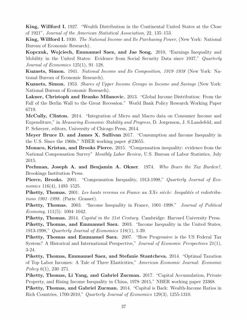
King, Willford I. 1927. “Wealth Distribution in the Continental United States at the Close

of 1921”, Journal of the American Statistical Association, 22, 135–153.

King, Willford I. 1930. The National Income and Its Purchasing Power, (New York: National

Bureau of Economic Research).

Kopczuk, Wojciech, Emmanuel Saez, and Jae Song. 2010, “Earnings Inequality and

Mobility in the United States: Evidence from Social Security Data since 1937,” Quarterly

Journal of Economics 125(1), 91–128.

Kuznets, Simon. 1941. National Income and Its Composition, 1919–1938 (New York: Na-

tional Bureau of Economic Research).

Kuznets, Simon. 1953. Shares of Upper Income Groups in Income and Savings (New York:

National Bureau of Economic Research).

Lakner, Christoph and Branko Milanovic. 2013. “Global Income Distribution: From the

Fall of the Berlin Wall to the Great Recession.” World Bank Policy Research Working Paper

6719.

McCully, Clinton. 2014. “Integration of Micro and Macro data on Consumer Income and

Expenditure,” in Measuring Economic Stability and Progress, D. Jorgenson, J. S.Landefeld, and

P. Schreyer, editors, University of Chicago Press, 2014.

Meyer Bruce D. and James X. Sullivan 2017. “Consumption and Income Inequality in

the U.S. Since the 1960s,” NBER working paper #23655.

Monaco, Kristan, and Brooks Pierce. 2015. “Compensation inequality: evidence from the

National Compensation Survey” Monthly Labor Review, U.S. Bureau of Labor Statistics, July

2015.

Pechman, Joseph A. and Benjamin A. Okner. 1974. Who Bears the Tax Burden?,

Brookings Institution Press.

Pierce, Brooks. 2001. “Compensation Inequality, 1913-1998,” Quarterly Journal of Eco-

nomics 116(4), 1493–1525.

Piketty, Thomas. 2001. Les hauts revenus en France au XXe siecle: Inegalites et redistribu-

tions 1901–1998. (Paris: Grasset).

Piketty, Thomas. 2003. “Income Inequality in France, 1901–1998.” Journal of Political

Economy, 111(5): 1004–1042.

Piketty, Thomas. 2014. Capital in the 21st Century. Cambridge: Harvard University Press.

Piketty, Thomas, and Emmanuel Saez. 2003. “Income Inequality in the United States,

1913-1998,” Quarterly Journal of Economics 118(1), 1-39.

Piketty, Thomas and Emmanuel Saez. 2007. “How Progressive is the US Federal Tax

System? A Historical and International Perspective,” Journal of Economic Perspectives 21(1),

3-24.

Piketty, Thomas, Emmanuel Saez, and Stefanie Stantcheva. 2014. “Optimal Taxation

of Top Labor Incomes: A Tale of Three Elasticities,” American Economic Journal: Economic

Policy 6(1), 230–271.

Piketty, Thomas, Li Yang, and Gabriel Zucman. 2017. “Capital Accumulation, Private

Property, and Rising Income Inequality in China, 1978–2015,” NBER working paper 23368.

Piketty, Thomas, and Gabriel Zucman. 2014. “Capital is Back: Wealth-Income Ratios in

Rich Countries, 1700-2010,” Quarterly Journal of Economics 129(3), 1255-1310.

37

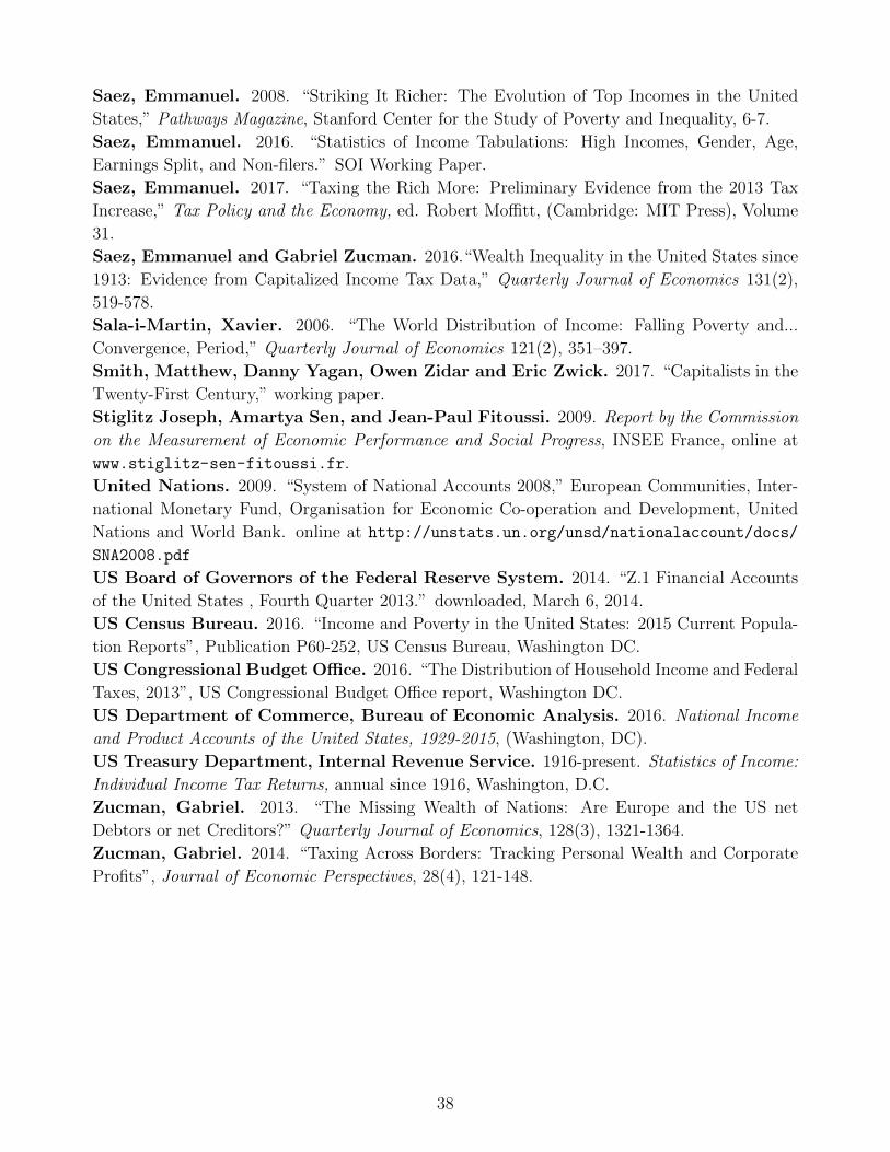
Saez, Emmanuel. 2008. “Striking It Richer: The Evolution of Top Incomes in the United

States,” Pathways Magazine, Stanford Center for the Study of Poverty and Inequality, 6-7.

Saez, Emmanuel. 2016. “Statistics of Income Tabulations: High Incomes, Gender, Age,

Earnings Split, and Non-filers.” SOI Working Paper.

Saez, Emmanuel. 2017. “Taxing the Rich More: Preliminary Evidence from the 2013 Tax

Increase,” Tax Policy and the Economy, ed. Robert Moffitt, (Cambridge: MIT Press), Volume

31.

Saez, Emmanuel and Gabriel Zucman. 2016.“Wealth Inequality in the United States since

1913: Evidence from Capitalized Income Tax Data,” Quarterly Journal of Economics 131(2),

519-578.

Sala-i-Martin, Xavier. 2006. “The World Distribution of Income: Falling Poverty and...

Convergence, Period,” Quarterly Journal of Economics 121(2), 351–397.

Smith, Matthew, Danny Yagan, Owen Zidar and Eric Zwick. 2017. “Capitalists in the

Twenty-First Century,” working paper.

Stiglitz Joseph, Amartya Sen, and Jean-Paul Fitoussi. 2009. Report by the Commission

on the Measurement of Economic Performance and Social Progress, INSEE France, online at

www.stiglitz-sen-fitoussi.fr.

United Nations. 2009. “System of National Accounts 2008,” European Communities, Inter-

national Monetary Fund, Organisation for Economic Co-operation and Development, United

Nations and World Bank. online at http://unstats.un.org/unsd/nationalaccount/docs/

SNA2008.pdf

US Board of Governors of the Federal Reserve System. 2014. “Z.1 Financial Accounts

of the United States , Fourth Quarter 2013.” downloaded, March 6, 2014.

US Census Bureau. 2016. “Income and Poverty in the United States: 2015 Current Popula-

tion Reports”, Publication P60-252, US Census Bureau, Washington DC.

US Congressional Budget Office. 2016. “The Distribution of Household Income and Federal

Taxes, 2013”, US Congressional Budget Office report, Washington DC.

US Department of Commerce, Bureau of Economic Analysis. 2016. National Income

and Product Accounts of the United States, 1929-2015, (Washington, DC).

US Treasury Department, Internal Revenue Service. 1916-present. Statistics of Income:

Individual Income Tax Returns, annual since 1916, Washington, D.C.

Zucman, Gabriel. 2013. “The Missing Wealth of Nations: Are Europe and the US net

Debtors or net Creditors?” Quarterly Journal of Economics, 128(3), 1321-1364.

Zucman, Gabriel. 2014. “Taxing Across Borders: Tracking Personal Wealth and Corporate

Profits”, Journal of Economic Perspectives, 28(4), 121-148.

38

TABLE I: The Distribution of National Income in the United States in 2014

Income group Number of adults

Income threshold

Average income Income share Income

thresholdAverage income Income share

Full Population 234,400,000 $64,600 100% $64,600 100%

Bottom 50% 117,200,000 $16,200 12.5% $24,900 19.3%

Bottom 20% (P0-P20) 46,880,000 $5,400 1.7% $13,100 4.1%

Next 30% (P20-P50) 70,320,000 $12,800 $23,400 10.9% $22,700 $32,800 15.2%

Middle 40% (P50-P90) 93,760,000 $36,000 $65,300 40.4% $43,900 $67,200 41.6%

Top 10% 23,440,000 $119,000 $304,000 47.0% $110,000 $253,000 39.1%

Top 1% 2,344,000 $458,000 $1,310,000 20.2% $383,000 $1,010,000 15.7%

Top 0.1% 234,400 $1,960,000 $6,000,000 9.3% $1,520,000 $4,400,000 6.8%

Top 0.01% 23,440 $9,560,000 $28,100,000 4.4% $6,870,000 $20,300,000 3.1%

Top 0.001% 2,344 $47,200,000 $121,900,000 1.9% $34,300,000 $88,700,000 1.4%

Pre-tax national income Post-tax national income

Notes: This table reports statistics on the income distribution in the United States in 2014 for pre-tax national income and post-tax national income.

Pre-tax and post-tax national income match national income. The unit is the adult individual (aged 20 or above). Income is split equally among spouses.

Fractiles are defined relative to the total number of adults in the population. Pre-tax national income fractiles are ranked by pre-tax national income, and

post-tax national income fractiles are ranked by post-tax national income. Hence, the two sets of fractiles do not represent the same groups of individuals

due to re-ranking when switching from one income definition to another.

39

TABLE II: The Growth of National Income in the United States since World War II

Income group 1946-1980 1980-2014 1946-1980 1980-2014

Full Population 95% 61% 95% 61%

Bottom 50% 102% 1% 129% 21%

Bottom 20% (P0-P20) 109% -25% 179% 4%

Next 30% (P20-P50) 101% 7% 117% 26%

Middle 40% (P50-P90) 105% 42% 98% 49%

Top 10% 79% 121% 69% 113%

Top 1% 47% 204% 58% 194%

Top 0.1% 54% 320% 104% 298%

Top 0.01% 76% 453% 201% 423%

Top 0.001% 57% 636% 163% 616%

Pre-tax income growth Post-tax income growth

Notes: The table displays the cumulative real growth rates of pre-tax and post-tax national income per adult over two 34 years period: 1980 to 2014 and

1946 to 1980. Pre-tax and post-tax national income match national income. The unit is the adult individual (aged 20 or above). Fractiles are defined

relative to the total number of adults in the population. Income is split equally among spouses. Pre-tax national income fractiles are ranked by pre-tax

national income while post-tax national income fractiles are ranked by post-tax national income. We assume that bottom 50% and middle 40% incomes

grew at the same rate as average bottom 90% income over 1946-1962. The deflator used is the national income price deflator.

40

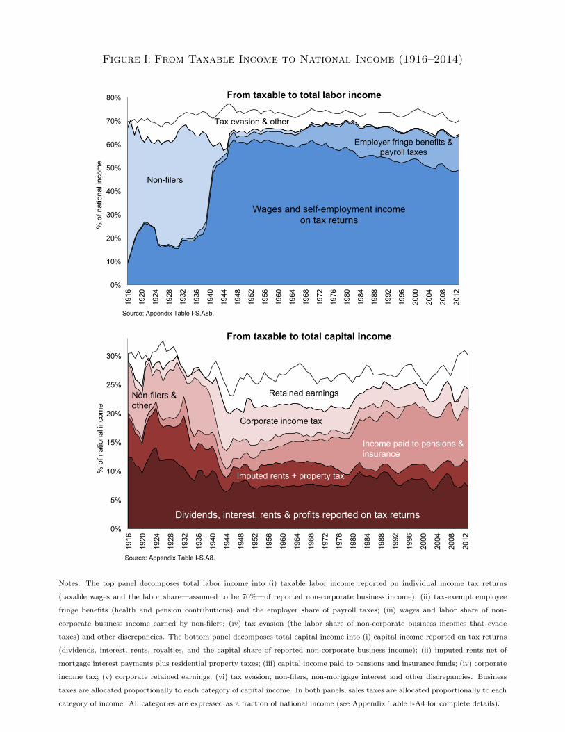
Figure I: From Taxable Income to National Income (1916–2014)

0%

10%

20%

30%

40%

50%

60%

70%

80%

1916

1920

1924

1928

1932

1936

1940

1944

1948

1952

1956

1960

1964

1968

1972

1976

1980

1984

1988

1992

1996

2000

2004

2008

2012

% o

f nat

iona

l inc

ome

From taxable to total labor income

Wages and self-employment income on tax returns

Employer fringe benefits & payroll taxes

Non-filers

Tax evasion & other

Source: Appendix Table I-S.A8b.

0%

5%

10%

15%

20%

25%

30%

1916

1920

1924

1928

1932

1936

1940

1944

1948

1952

1956

1960

1964

1968

1972

1976

1980

1984

1988

1992

1996

2000

2004

2008

2012

% o

f nat

iona

l inc

ome

From taxable to total capital income

Dividends, interest, rents & profits reported on tax returns

Imputed rents + property tax

Retained earnings

Income paid to pensions & insurance

Non-filers & other

Corporate income tax

Source: Appendix Table I-S.A8.

Notes: The top panel decomposes total labor income into (i) taxable labor income reported on individual income tax returns

(taxable wages and the labor share—assumed to be 70%—of reported non-corporate business income); (ii) tax-exempt employee

fringe benefits (health and pension contributions) and the employer share of payroll taxes; (iii) wages and labor share of non-

corporate business income earned by non-filers; (iv) tax evasion (the labor share of non-corporate business incomes that evade

taxes) and other discrepancies. The bottom panel decomposes total capital income into (i) capital income reported on tax returns

(dividends, interest, rents, royalties, and the capital share of reported non-corporate business income); (ii) imputed rents net of

mortgage interest payments plus residential property taxes; (iii) capital income paid to pensions and insurance funds; (iv) corporate

income tax; (v) corporate retained earnings; (vi) tax evasion, non-filers, non-mortgage interest and other discrepancies. Business

taxes are allocated proportionally to each category of capital income. In both panels, sales taxes are allocated proportionally to each

category of income. All categories are expressed as a fraction of national income (see Appendix Table I-A4 for complete details).

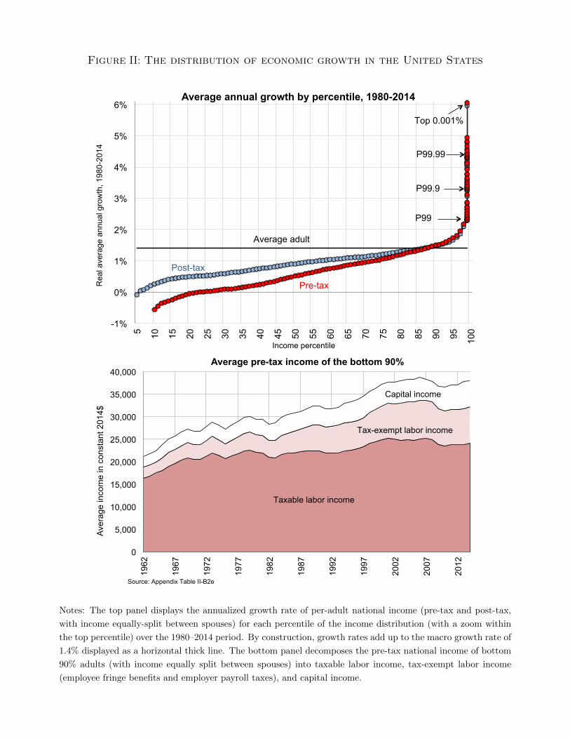
Figure II: The distribution of economic growth in the United States

-1%

0%

1%

2%

3%

4%

5%

6%

5 10

15

20

25

30

35

40

45

50

55

60

65

70

75

80

85

90

95

100

Rea

l ave

rage

ann

ual g

row

th, 1

980-

2014

Income percentile

Average annual growth by percentile, 1980-2014

Top 0.001%

Average adult

Pre-tax

Post-tax

P99

P99.9

P99.99

0

5,000

10,000

15,000

20,000

25,000

30,000

35,000

40,000

1962

1967

1972

1977

1982

1987

1992

1997

2002

2007

2012

Aver

age

inco

me

in c

onst

ant 2

014$

Average pre-tax income of the bottom 90%

Taxable labor income

Capital income

Tax-exempt labor income

Source: Appendix Table II-B2e

Notes: The top panel displays the annualized growth rate of per-adult national income (pre-tax and post-tax,

with income equally-split between spouses) for each percentile of the income distribution (with a zoom within

the top percentile) over the 1980–2014 period. By construction, growth rates add up to the macro growth rate of

1.4% displayed as a horizontal thick line. The bottom panel decomposes the pre-tax national income of bottom

90% adults (with income equally split between spouses) into taxable labor income, tax-exempt labor income

(employee fringe benefits and employer payroll taxes), and capital income.

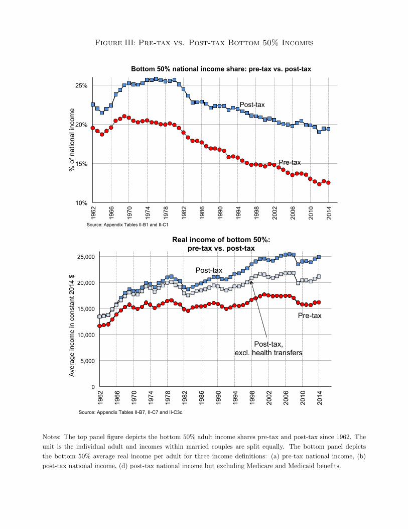
Figure III: Pre-tax vs. Post-tax Bottom 50% Incomes

10%

15%

20%

25% 19

62

1966

1970

1974

1978

1982

1986

1990

1994

1998

2002

2006

2010

2014

% o

f nat

iona

l inc

ome

Bottom 50% national income share: pre-tax vs. post-tax

Pre-tax

Post-tax

Source: Appendix Tables II-B1 and II-C1

0

5,000

10,000

15,000

20,000

25,000

1962

1966

1970

1974

1978

1982

1986

1990

1994

1998

2002

2006

2010

2014

Aver

age

inco

me

in c

onst

ant 2

014

$

Real income of bottom 50%: pre-tax vs. post-tax

Source: Appendix Tables II-B7, II-C7 and II-C3c.

Post-tax

Post-tax, excl. health transfers

Pre-tax

Notes: The top panel figure depicts the bottom 50% adult income shares pre-tax and post-tax since 1962. The

unit is the individual adult and incomes within married couples are split equally. The bottom panel depicts

the bottom 50% average real income per adult for three income definitions: (a) pre-tax national income, (b)

post-tax national income, (d) post-tax national income but excluding Medicare and Medicaid benefits.

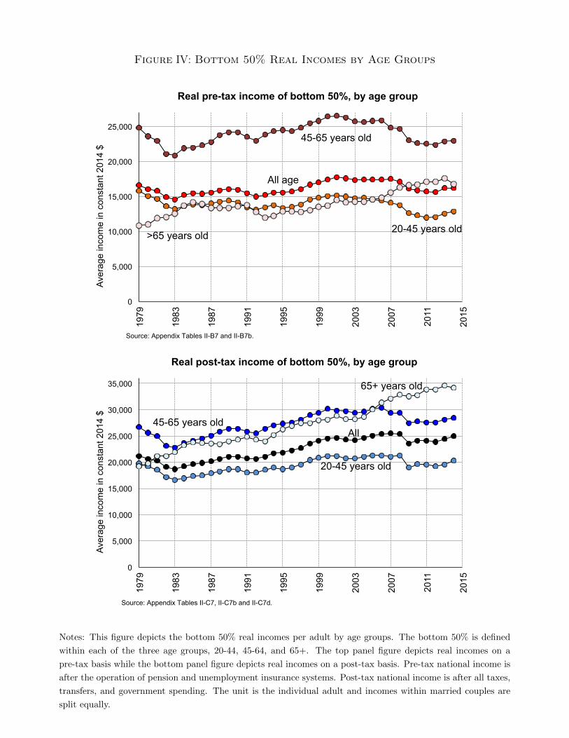
Figure IV: Bottom 50% Real Incomes by Age Groups

0

5,000

10,000

15,000

20,000

25,000

1979

1983

1987

1991

1995

1999

2003

2007

2011

2015

Aver

age

inco

me

in c

onst

ant 2

014

$ Real pre-tax income of bottom 50%, by age group

Source: Appendix Tables II-B7 and II-B7b.

All age

20-45 years old

45-65 years old

>65 years old

0

5,000

10,000

15,000

20,000

25,000

30,000

35,000

1979

1983

1987

1991

1995

1999

2003

2007

2011

2015

Aver

age

inco

me

in c

onst

ant 2

014

$

Real post-tax income of bottom 50%, by age group

Source: Appendix Tables II-C7, II-C7b and II-C7d.

All

20-45 years old

45-65 years old

65+ years old

Notes: This figure depicts the bottom 50% real incomes per adult by age groups. The bottom 50% is defined

within each of the three age groups, 20-44, 45-64, and 65+. The top panel figure depicts real incomes on a

pre-tax basis while the bottom panel figure depicts real incomes on a post-tax basis. Pre-tax national income is

after the operation of pension and unemployment insurance systems. Post-tax national income is after all taxes,

transfers, and government spending. The unit is the individual adult and incomes within married couples are

split equally.

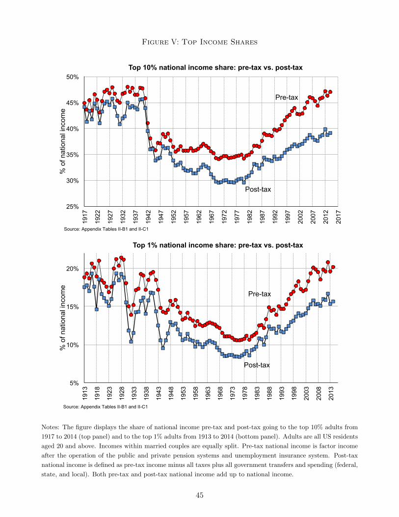
Figure V: Top Income Shares

25%

30%

35%

40%

45%

50% 19

17

1922

1927

1932

1937

1942

1947

1952

1957

1962

1967

1972

1977

1982

1987

1992

1997

2002

2007

2012

2017

% o

f nat

iona

l inc

ome

Top 10% national income share: pre-tax vs. post-tax

Pre-tax

Post-tax

Source: Appendix Tables II-B1 and II-C1

5%

10%

15%

20%

1913

1918

1923

1928

1933

1938

1943

1948

1953

1958

1963

1968

1973

1978

1983

1988

1993

1998

2003

2008

2013

% o

f nat

iona

l inc

ome

Top 1% national income share: pre-tax vs. post-tax

Pre-tax

Post-tax

Source: Appendix Tables II-B1 and II-C1

Notes: The figure displays the share of national income pre-tax and post-tax going to the top 10% adults from

1917 to 2014 (top panel) and to the top 1% adults from 1913 to 2014 (bottom panel). Adults are all US residents

aged 20 and above. Incomes within married couples are equally split. Pre-tax national income is factor income

after the operation of the public and private pension systems and unemployment insurance system. Post-tax

national income is defined as pre-tax income minus all taxes plus all government transfers and spending (federal,

state, and local). Both pre-tax and post-tax national income add up to national income.

45

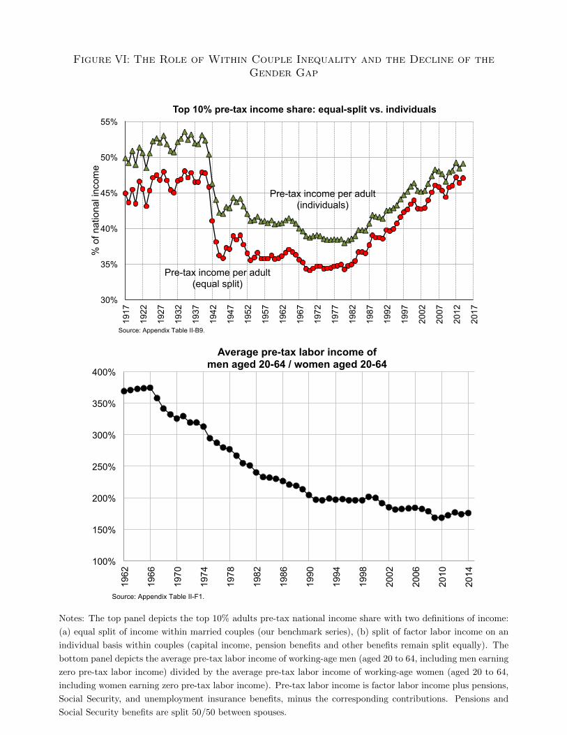
Figure VI: The Role of Within Couple Inequality and the Decline of theGender Gap

30%

35%

40%

45%

50%

55% 19

17

1922

1927

1932

1937

1942

1947

1952

1957

1962

1967

1972

1977

1982

1987

1992

1997

2002

2007

2012

2017

% o

f nat

iona

l inc

ome

Top 10% pre-tax income share: equal-split vs. individuals

Pre-tax income per adult (individuals)

Source: Appendix Table II-B9.

Pre-tax income per adult (equal split)

100%

150%

200%

250%

300%

350%

400%

1962

1966

1970

1974

1978

1982

1986

1990

1994

1998

2002

2006

2010

2014

Average pre-tax labor income of men aged 20-64 / women aged 20-64

Source: Appendix Table II-F1.

Notes: The top panel depicts the top 10% adults pre-tax national income share with two definitions of income:

(a) equal split of income within married couples (our benchmark series), (b) split of factor labor income on an

individual basis within couples (capital income, pension benefits and other benefits remain split equally). The

bottom panel depicts the average pre-tax labor income of working-age men (aged 20 to 64, including men earning

zero pre-tax labor income) divided by the average pre-tax labor income of working-age women (aged 20 to 64,

including women earning zero pre-tax labor income). Pre-tax labor income is factor labor income plus pensions,

Social Security, and unemployment insurance benefits, minus the corresponding contributions. Pensions and

Social Security benefits are split 50/50 between spouses.

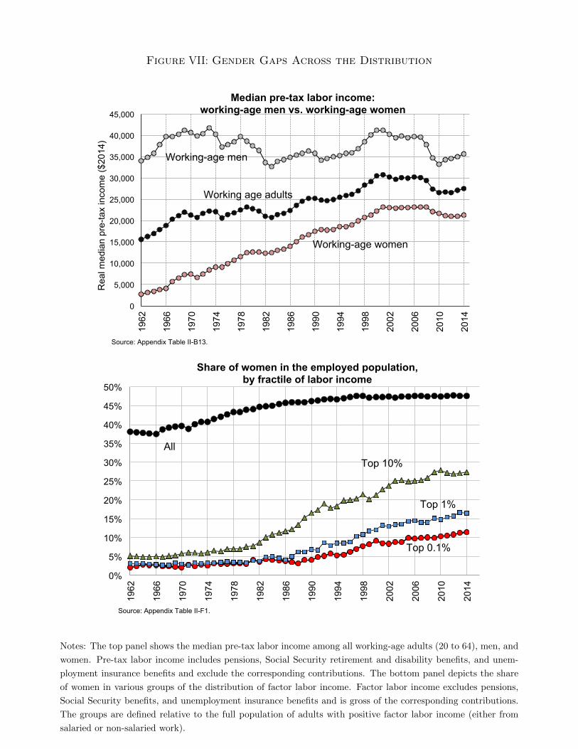
Figure VII: Gender Gaps Across the Distribution

0

5,000

10,000

15,000

20,000

25,000

30,000

35,000

40,000

45,000

1962

1966

1970

1974

1978

1982

1986

1990

1994

1998

2002

2006

2010

2014

Rea

l med

ian

pre-

tax

inco

me

($20

14)

Median pre-tax labor income: working-age men vs. working-age women

Source: Appendix Table II-B13.

Working-age men

Working-age women

Working age adults

0%

5%

10%

15%

20%

25%

30%

35%

40%

45%

50%

1962

1966

1970

1974

1978

1982

1986

1990

1994

1998

2002

2006

2010

2014

Share of women in the employed population, by fractile of labor income

Source: Appendix Table II-F1.

Top 10%

Top 0.1%

Top 1%

All

Notes: The top panel shows the median pre-tax labor income among all working-age adults (20 to 64), men, and

women. Pre-tax labor income includes pensions, Social Security retirement and disability benefits, and unem-

ployment insurance benefits and exclude the corresponding contributions. The bottom panel depicts the share

of women in various groups of the distribution of factor labor income. Factor labor income excludes pensions,

Social Security benefits, and unemployment insurance benefits and is gross of the corresponding contributions.

The groups are defined relative to the full population of adults with positive factor labor income (either from

salaried or non-salaried work).

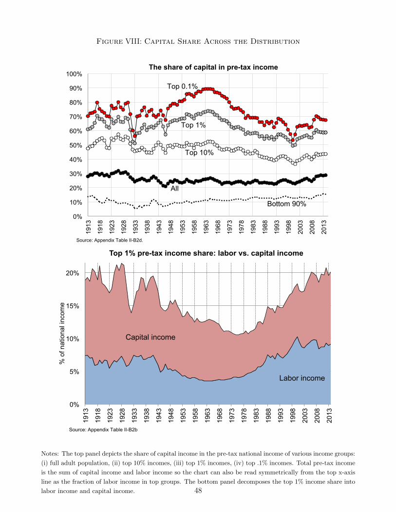
Figure VIII: Capital Share Across the Distribution

0%

10%

20%

30%

40%

50%

60%

70%

80%

90%

100%

1913

1918

1923

1928

1933

1938

1943

1948

1953

1958

1963

1968

1973

1978

1983

1988

1993

1998

2003

2008

2013

The share of capital in pre-tax income

Top 0.1%

Top 1%

Top 10%

All

Bottom 90%

Source: Appendix Table II-B2d.

0%

5%

10%

15%

20%

1913

1918

1923

1928

1933

1938

1943

1948

1953

1958

1963

1968

1973

1978

1983

1988

1993

1998

2003

2008

2013

% o

f nat

iona

l inc

ome

Top 1% pre-tax income share: labor vs. capital income

Source: Appendix Table II-B2b

Capital income

Labor income

Notes: The top panel depicts the share of capital income in the pre-tax national income of various income groups:

(i) full adult population, (ii) top 10% incomes, (iii) top 1% incomes, (iv) top .1% incomes. Total pre-tax income

is the sum of capital income and labor income so the chart can also be read symmetrically from the top x-axis

line as the fraction of labor income in top groups. The bottom panel decomposes the top 1% income share into

labor income and capital income. 48

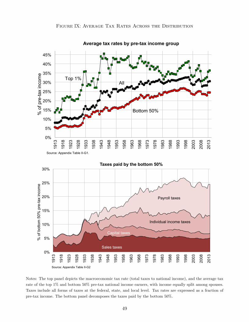
Figure IX: Average Tax Rates Across the Distribution

0%

5%

10%

15%

20%

25%

30%

35%

40%

45% 19

13

1918

1923

1928

1933

1938

1943

1948

1953

1958

1963

1968

1973

1978

1983

1988

1993

1998

2003

2008

2013

% o

f pre

-tax

inco

me

Average tax rates by pre-tax income group

Source: Appendix Table II-G1.

All

Bottom 50%

Top 1%

0%

5%

10%

15%

20%

25%

30%

1913

1918

1923

1928

1933

1938

1943

1948

1953

1958

1963

1968

1973

1978

1983

1988

1993

1998

2003

2008

2013

% o

f bot

tom

50%

pre

-tax

inco

me

Taxes paid by the bottom 50%

Capital taxes

Sales taxes

Individual income taxes

Payroll taxes

Source: Appendix Table II-G2

Notes: The top panel depicts the macroeconomic tax rate (total taxes to national income), and the average tax

rate of the top 1% and bottom 50% pre-tax national income earners, with income equally split among spouses.

Taxes include all forms of taxes at the federal, state, and local level. Tax rates are expressed as a fraction of

pre-tax income. The bottom panel decomposes the taxes paid by the bottom 50%.

49

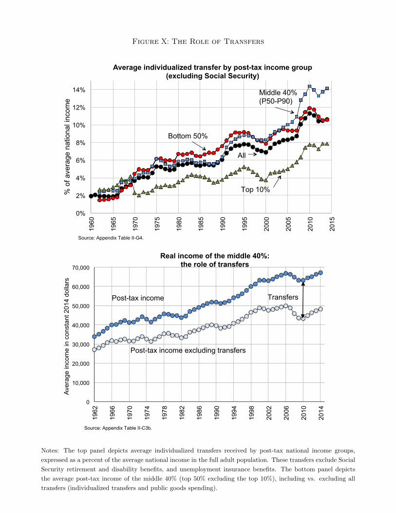
Figure X: The Role of Transfers

0%

2%

4%

6%

8%

10%

12%

14% 19

60

1965

1970

1975

1980

1985

1990

1995

2000

2005

2010

2015

% o

f ave

rage

nat

iona

l inc

ome

Average individualized transfer by post-tax income group (excluding Social Security)

Source: Appendix Table II-G4.

Middle 40% (P50-P90)

Bottom 50%

Top 10%

All

0

10,000

20,000

30,000

40,000

50,000

60,000

70,000

1962

1966

1970

1974

1978

1982

1986

1990

1994

1998

2002

2006

2010

2014

Aver

age

inco

me

in c

onst

ant 2

014

dolla

rs

Real income of the middle 40%: the role of transfers

Source: Appendix Table II-C3b.

Post-tax income excluding transfers

Post-tax income Transfers

Notes: The top panel depicts average individualized transfers received by post-tax national income groups,

expressed as a percent of the average national income in the full adult population. These transfers exclude Social

Security retirement and disability benefits, and unemployment insurance benefits. The bottom panel depicts

the average post-tax income of the middle 40% (top 50% excluding the top 10%), including vs. excluding all

transfers (individualized transfers and public goods spending).

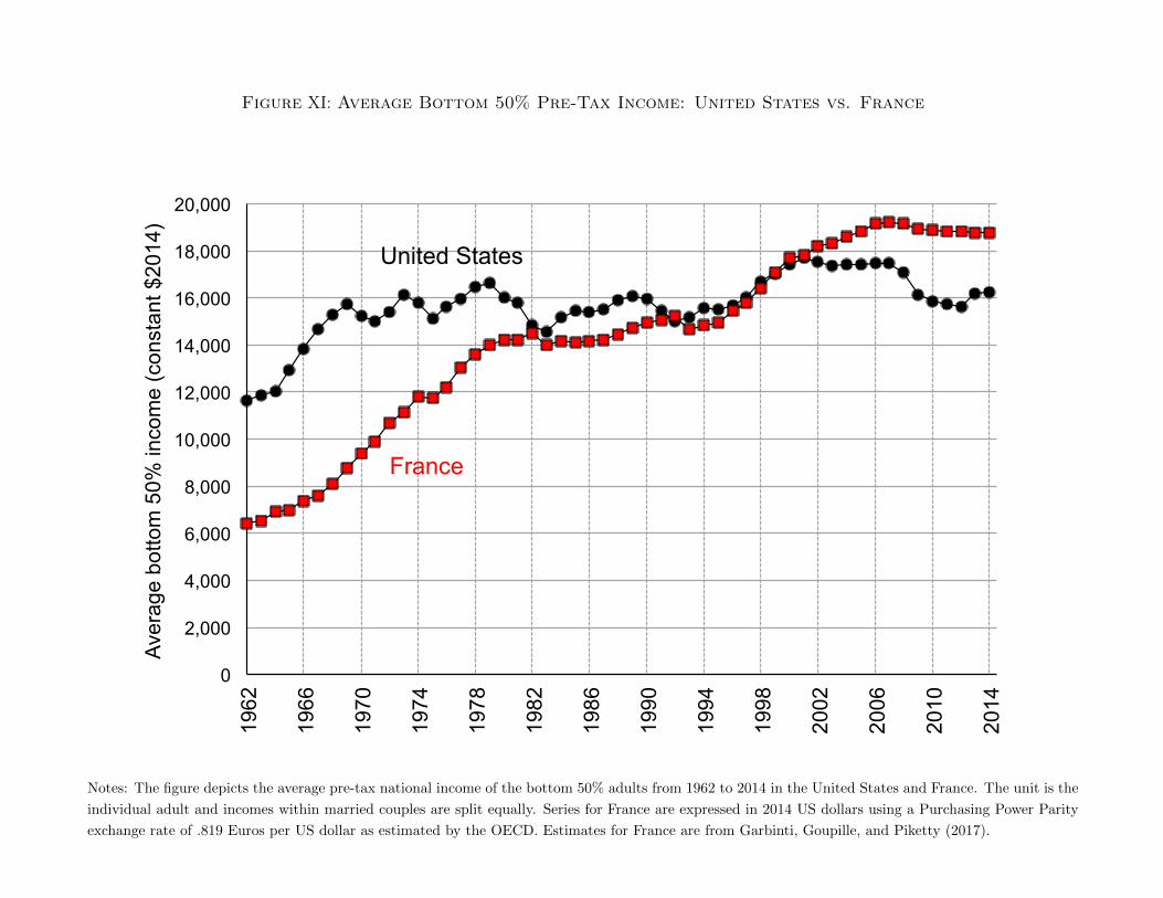
Figure XI: Average Bottom 50% Pre-Tax Income: United States vs. France

0

2,000

4,000

6,000

8,000

10,000

12,000

14,000

16,000

18,000

20,000

1962

1966

1970

1974

1978

1982

1986

1990

1994

1998

2002

2006

2010

2014

Aver

age

botto

m 5

0% in

com

e (c

onst

ant $

2014

)

United States

France

Notes: The figure depicts the average pre-tax national income of the bottom 50% adults from 1962 to 2014 in the United States and France. The unit is the

individual adult and incomes within married couples are split equally. Series for France are expressed in 2014 US dollars using a Purchasing Power Parity

exchange rate of .819 Euros per US dollar as estimated by the OECD. Estimates for France are from Garbinti, Goupille, and Piketty (2017).