DISTRIBUTION OF THE WEALTH OF THE RICHEST PERSONS IN THE WORLD

DISTRIBUTION OF THE WEALTH

OF THE RICHEST PERSONS IN THE WORLD

ADAM ČABLAa,*, FILIP HABARTAa

[email protected], [email protected]

a University of Economics in Prague, Faculty of Informatics and Statistics, Department of Statistics and

Probability, W. Churchill Sq. 4, Prague, Czech Republic

Abstract

The aim of this paper is to examine the probability distribution of wealth of the richest persons in the

world based on estimates from the CEOWORLD magazine’s rich list for March 2019. Since one can

safely assume that there are a tiny number of people out of the whole world’s population in this list,

we basically deal with the very right tail of the wealth distribution, which should according to the

Pickands-Balkema-de Haan theorem follow a generalized Pareto distribution. We discuss in this paper

not only different estimates of this distribution with an emphasis on the shape parameter per se but

also their behavior throughout bootstrap samples. Among the main findings is the observation based

on the maximum to sum plot and parametric estimates that there is high probability of infinite

variance. This could have a serious impact on estimates of inequality measures. The whole distribution

follows nearly a Pareto distribution, whereas the very right tail is closer to an exponential. The

bootstrap technique confirms that maximum likelihood estimates are almost normally distributed, but

they overestimate variance. Estimates via the method of L-moments diverge from the normal

distribution. The correlation of the parameter estimates is moderately negative, which is demonstrated

in a simultaneous confidence region.

Key words

CEOWORLD magazine’s Rich List, Pickands-Balkema-de Haan theorem, generalized Pareto

distribution, parameter estimates, bootstrap

JEL classification

C13, C15

1. Introduction

Wealth and income distributions are widely debated and researched topic both in scientific

and popular literature. They are implicated in discussions of general wealth of populations as

well as in discussions of economic equality and fairness with perceived need to re-distribute.

One of the most popular measurements of the wealth and income distributions is Gini

coefficient, other measures are used in evaluating the right tail of the income or wealth

distributions. Many of the currently used measures of inequality have estimates based on

assumption of the finite variance and don’t fare well under heavy-tailed distributions (Cowell

and Flachaire, 2007, Fontanari et al., 2018), so the discussion whether income distribution has

finite variance is of high importance in economics.

The right tail is a vague term describing the part of the distribution higher than some

specified threshold. In the context of the wealth distribution, the right tail has the meaning of

the distribution of the wealth among sufficiently rich people. Since wealth distribution is

usually heavy-tailed (for the definition of heavy-tailed distribution see e.g. Foss et al, 2013),

its right tail has properties important for the whole distribution. Among most popular heavy-

tailed distributions used in modelling of income or wealth distributions are log-normal and

Pareto distributions. There is however difference between log-normal and Pareto distribution

22nd International Scientific Conference on Applications of Mathematics and Statistics in Economics (AMSE 2019)

Copyright © 2019, the Authors. Published by Atlantis Press. This is an open access article under the CC BY-NC license (http://creativecommons.org/licenses/by-nc/4.0/).

Atlantis Studies in Uncertainty Modelling, volume 2

158

in the speed of decline of the density, which was recently discussed in connection with the

wealth distribution e.g. in Jaguelski et al. (2017) or Campolieti (2018).

The heaviness of the distribution can be estimated as a tail index via several methods, some

specific, e.g. Pickands or Hill estimators. More general method is an estimate of specific

distribution and calculating tail index from this.

In this paper we have an aim to take a different angle of view – to start with the description

of the basics of extreme value theory (EVT) and move onto its relevance to the discussion of

the distribution of the wealth of the richest people in the world. Then we continue with

estimating this distribution and inference within two methods used for the estimates –

maximum likelihood and L-moments.

2. Data and software

We use data obtained from the CEO World magazine’s Rich List1, that contains estimated

net worth of wealth of the 500 richest persons in the world. For the sake of simplicity, we

truncated the data at 4 billion dollars, so in other words we use the list of people having

(estimated) more than 4 billion dollars – there are 483 such persons in the dataset.

Table 1: Descriptive statistics of the wealth of 483 richest persons in the world

Statistics Value in billions of $

Minimum 4.01

First quartile 4.88

Median 6.57

Third Quartile 11.40

Maximum 140.00

Mean 10.75

Variance 162.30

Source: the authors.

Figure 1: Boxplot of the wealth of 483 richest persons in the world


Table 1 contains basic descriptive statistics and Figure 1 shows the distribution of the

wealth as a boxplot. The four richest persons are pointed out. Summary statistics and figures

point out toward heavy-tailed distribution as expected.

Software used throughout the paper is R (R Core Team, 2018) with packages extRemes

(Gilleland and Katz, 2016) for parameter estimates and ellipse (Murdoch and Chow, 2018) for

simultaneous confidence region estimate.

1 Available at https://ceoworld.biz/2018/05/30/rich-list/ (accessed on 2019-03-06).


159

https://ceoworld.biz/2018/05/30/rich-list/

3. Extreme value theory

EVT is a branch of mathematic statistics dealing with the probability distribution of the

extremes. There are two different, even though connected, approaches based on two different

theorems. EVT is used in many different fields such as insurance, hydrology, meteorology or

finance.

First theorem used in EVT is Fisher-Tippet-Gnedenko theorem (Gnedenko, 1943) basically

stating, that if the distribution of maximas of independent identically distributed random

variables (e.g. maximas in random samples from the same distribution) converges, it

converges to the generalized extreme value distribution (GEVD), that can be differed to

Fréchet, Weibull or Gumbel distributions.

Second theorem used in EVT is Pickands-Balkema-de Haan theorem (de Haan and

Balkema, 1974; Pickands, 1975) stating following:

“Let X1, X2, … be a sequence of independent and identically distributed random variables

with distribution function F. Random variables for which X > µ has excess distribution

function

( ) ( )F y P X y X , (1)

where X is a random variable, µ is given threshold, y = x – µ are excesses. Then

,( ) ( )F y G y

, (2)

where Gζ,σ(y) is cumulative distribution function of generalized Pareto distribution (GPD)

written in formula 3.

1/

, ,

( )1 1 for 0

( )

1 exp for 0

x

G xx

(3)

The three parameters of the GPD are threshold (sometimes referred to as a location)

parameter µ, scale parameter σ and shape parameter ζ. Shape parameter basically decide

whether probability density decreases slower or faster than exponential distribution and if its

value is 0, then the right tail is exponentially distributed. When ζ > 0, then the right tail

decreases faster than the exponential distribution and it can be classified as heavy-tailed. With

ζ > 0 and µ = σ/ζ, the GPD is equivalent to Pareto distribution with parametrization xm = σ/ζ

and α = 1/ζ with following cumulative density function

, 1m

mx

xF

x

. (4)

More generally 1/ζ can be viewed as an estimate of tail index mentioned above.

GPD has finite expectation if ζ < 1, finite variance if ζ < 0.5, finite skewness if ζ < 1/3 and

finite kurtosis if ζ < 1/4.

There is a more general relation between underlying distribution, its maxima distributions

per Fisher-Tippet-Gnedenko theorem and its right tail behavior expressed as a GPD. These

are expressed as domains of attraction of the GEVD and some of well-known distributions

that have specific domains of attraction are mentioned in Table 2.

,

.


160

Table 2: Domains of attraction for some distributions

Situation Domain of attraction Tail behavior Distribution examples

ζ > 0 Fréchet Polynomial, possibly Pareto Pareto, Cauchy, Student’s

ζ < 0 Weibull Finite end-point Uniform, Beta

ζ = 0 Gumbel Exponential Normal, log-normal, exponential, gamma


The “true” distribution of the wealth of the richest persons is usually discussed to be

truncated lognormal (Campolieti, 2018) or Paretian (Jaguelski et al., 2017; or Capehart, 2014)

or it can be modelled by different functions, e.g. by Lorenz curve (Wang and You, 2016).

Starting from the EVT and more specifically Pickands-Balkema-de Haan theorem we can

view wealth of an individual person following unknown underlying probability distribution

and the world population as a sample from this distribution. Then following this logic, we can

view the very right tail of the wealth distribution as an excess distribution that will follow

GPD if the threshold is sufficiently high. We think that having 483 richest persons from the

world’s population exceeding 7.5 billion people and the threshold of 4 billion dollars is

sufficiently high and this approach is justifiable not only on empirical but also on theoretical

ground.

3.1. Estimates of GPD

When estimating GPD, researchers usually stand before several possible issues. First of

them is selection of an appropriate estimation method, method of inference and within these

methods, selection of the sufficiently high threshold. There are methods specific to the GPD,

such as de Haan method (Simiu and Heckert, 1996) and there are more general approaches,

e.g. maximum likelihood estimate (MLE), method of probability weighted moments (PWM)

or method of L-moments (MLM).

In this paper we chose MLE and MLM – first because of its well-known nature and

asymptotic normality of the parameter estimates, where we use inverse Hessian matrix as an

estimate of covariance matrix of parameter estimates. If ζ > 0.5, the MLE produces unbiased

estimates, but its asymptotic properties are questionable (due to infinite variance). Second one

because of its robustness and possibility to obtain unbiased estimates under the condition that

the first moment is finite, that is if ζ < 1.

Because as we will see further in chapter 4 the point estimates of ζ are higher than 0.5 but

lower than 1, we use bootstrapping methods to show the properties of the parameter estimates

and its 95 % confidence intervals and compare them to the estimates obtained via normal

approximation within MLE. We also discus correlation of the parameter estimates within

MLE and even within MLM. We use 200 000 bootstrap samples.

Another issue is usually threshold selection. As for this we follow standard graphical

procedure, that is evaluating the figure plotting mean over threshold against the threshold and

parameter estimates against the threshold. We discuss some possible implications but use the

original 4 billion dollars as a threshold, nevertheless.

4. Results

4.1. Maximum to Sum plot

As a first step in evaluating distribution of the top wealth we start with Maximum to Sum

plot (Cirillo and Taleb, 2016) as a tool to evaluate existence of moments of the underlying

distributions. For a sequence (X1, X2, …, Xn) of nonnegative independent identically

distributed random variables, if for k = 1, 2, 3,…, holds E(Xk) < ∞, then follows


161

1

1

0

where and max ,...,

nk k k

n n n

nk k k k k

n i n n

i

R M S

S X M X X

(5)

Figure 2 shows 100 reshuffled paths of the ratio of maximum to sum from the original data

for first 4 moments – since the path is dependent on the order in the sample and since there is

no clear way to sort them (like e.g. in time series data) we used this approach to visualize the

data. Figure 3 shows 100 possible paths based on 100 bootstrap samples. In our opinion it is

clear, that the ratio converges to 0 for k = 1 and does not converge to 0 for k = 3 and 4. As for

the second moment, the ratio seems to converge rather slowly and so the second moment may

not be finite. This suggests, that ζ is higher than 1/3 as third moment is not finite and possibly

higher than 0.5 as second moment is possibly not finite. The bootstrap method has its limit

here in the fact that all moments are finite in the sample and hence the mean final values in

Figure 3 are substantially lower than final values in Figure 2.

Figure 2: Maximum to Sum plot for 100 different paths


Figure 3: Maximum to Sum plot for 100 bootstrap distributions


,

.


162

4.2. Relation of mean and parameter estimates to selected threshold

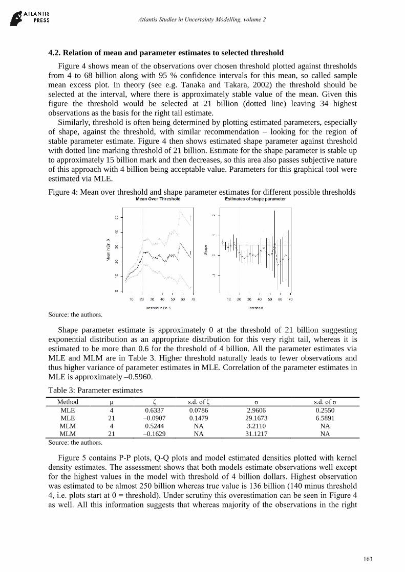
Figure 4 shows mean of the observations over chosen threshold plotted against thresholds

from 4 to 68 billion along with 95 % confidence intervals for this mean, so called sample

mean excess plot. In theory (see e.g. Tanaka and Takara, 2002) the threshold should be

selected at the interval, where there is approximately stable value of the mean. Given this

figure the threshold would be selected at 21 billion (dotted line) leaving 34 highest

observations as the basis for the right tail estimate.

Similarly, threshold is often being determined by plotting estimated parameters, especially

of shape, against the threshold, with similar recommendation – looking for the region of

stable parameter estimate. Figure 4 then shows estimated shape parameter against threshold

with dotted line marking threshold of 21 billion. Estimate for the shape parameter is stable up

to approximately 15 billion mark and then decreases, so this area also passes subjective nature

of this approach with 4 billion being acceptable value. Parameters for this graphical tool were

estimated via MLE.

Figure 4: Mean over threshold and shape parameter estimates for different possible thresholds


Shape parameter estimate is approximately 0 at the threshold of 21 billion suggesting

exponential distribution as an appropriate distribution for this very right tail, whereas it is

estimated to be more than 0.6 for the threshold of 4 billion. All the parameter estimates via

MLE and MLM are in Table 3. Higher threshold naturally leads to fewer observations and

thus higher variance of parameter estimates in MLE. Correlation of the parameter estimates in

MLE is approximately –0.5960.

Table 3: Parameter estimates

Method µ ζ s.d. of ζ σ s.d. of σ

MLE 4 0.6337 0.0786 2.9606 0.2550

MLE 21 –0.0907 0.1479 29.1673 6.5891

MLM 4 0.5244 NA 3.2110 NA

MLM 21 –0.1629 NA 31.1217 NA


Figure 5 contains P-P plots, Q-Q plots and model estimated densities plotted with kernel

density estimates. The assessment shows that both models estimate observations well except

for the highest values in the model with threshold of 4 billion dollars. Highest observation

was estimated to be almost 250 billion whereas true value is 136 billion (140 minus threshold

4, i.e. plots start at 0 = threshold). Under scrutiny this overestimation can be seen in Figure 4

as well. All this information suggests that whereas majority of the observations in the right


163

tail follow approximately Pareto distribution (since 2.9606/0.6337 = 4.67, close to threshold

4), the very right part is closer to exponential distribution.

Figure 5: Evaluation of the model quality (threshold of 4 billion $ on the left side)


4.3. Bootstrap estimates

To evaluate MLE we can use their asymptotic normality and estimated covariance matrix,

that yields estimate of variance of the parameter estimates. However, since the underlying

distribution probably does not have finite variance, we decided to confront these inductions

with 200 000 bootstrap samples and find out distribution and several other information from

these. Moreover, to make same basic induction about MLM estimates we used the same

technique. Sampling was done from the original data (denoted as (1) in the tables) and then

from the estimated models (denoted as (2) in the tables). Since data have finite variance and

models do not, we were also looking for the difference in the estimated characteristics.

Table 4 shows original estimates with those from bootstrap samples. Estimate of the shape

parameter seems to be slightly overestimated and scale parameter underestimated, which

seems logical given their negative correlation. Standard deviations seem slightly

overestimated whereas correlation seems underestimated (overestimated in absolute value) in

comparison with the second bootstrap procedure (bootstrapping from the model).

Table 4: Estimates based on bootstrapping for MLE

Parameter Estimate Estimated

95% C.I.

B.mean

est.(1) B. 95% C.I.(1)

B. mean

est.(2) B. 95% C.I.(2)

ζ 0.6337 (0.480; 0.788) 0.6304 (0.494; 0.787) 0.6296 (0.485; 0.777)

σ 2.9606 (2.461; 3.460) 2.9770 (2.485; 3.537) 2.9775 (2.524; 3.486)

s.d.(ζ) 0.0786 NA 0.0785 (0.071; 0.086) 0.0743 (0.067; 0.082)

s.d.(σ) 0.2550 NA 0.2560 (0.217; 0.300) 0.2447 (0.210; 0.283)

Corr. –0.5960 NA –0.5969 (–0.640; –0.556) –0.5553 (–0.606; –0.507)



164

Table 5: Estimates based on bootstrapping for MLM

Parameter Estimate Estimated

95% C.I.

B.mean

est.(1) B. 95% C.I.(1)

B. mean

est.(2) B. 95% C.I.(2)

ζ 0.5244 NA 0.5184 (0.435; 0.591) 0.5076 (0.374; 0.680)

σ 3.2110 NA 3.2390 (2.767; 3.769) 3.2479 (2.728; 3.788)


Table 5 contains estimates of parameters obtained via MLM and calculated bootstrap

confidence intervals both from the data and from the model. Shape parameter seems to be

slightly overestimated, especially when compared to the bootstrap samples from the model,

whereas opposite seems to be true for the scale parameter – the opposite of what have been

seen in the MLE. Accuracy of both methods (MLE and MLM) as measured by the width of

the confidence intervals seems to be comparable. Only one outstanding exception is in the

confidence interval for shape parameter obtained from bootstrap samples from data – interval

for the MLM estimate seems narrow in comparison to others, but also to the one obtained

from the bootstrap samples from the MLM model. This difference can be partially due to the

difference in variance in the sample (finite) and in the model (infinite).

Histograms for the estimates of shape parameter based on 200 000 bootstrap samples are in

Figure 6 for the MLE and in Figure 7 for the MLM. MLE estimates follow normal

distribution well but have distribution with lower variance than estimated by the original

model – the higher difference is seen in the bootstrap from the original sample than in the

bootstrap from the model (s.d. 0.0700 and 0.0745 vs. 0.0786). Despite this difference

estimated confidence intervals are similar as seen in Table 4. In MLM estimates in the

bootstrap samples from the original sample we can see there is slight divergence from the

normality – estimated normal distribution is moved to the left when compared to the kernel

density estimate. In the estimates from the model the divergence is much more pronounced

with higher modus and higher variance for normal estimate than for bootstrap estimate (s.d.

0.0399 vs. 0.0775 in the bootstrap from sample than from model). This difference is also

visible in the estimated confidence intervals in Table 5.

Figure 6: Histogram of bootstrap shape parameter estimates, from sample and model, MLE



165

Figure 7: Histogram of bootstrap shape parameter estimates, from sample and model, MLM


Maximum likelihood estimates suggest, that the distribution of top incomes does not have

finite variance whereas estimates done via method of L-moments do not provide clear

evidence on any of the possibilities.

Table 6 holds correlation estimates obtained through different methods. There is original

estimate from the MLE model, then there are means of correlations of 200 000 bootstrap

samples and following are inter-sample correlations – correlations calculated in the 200 000

bootstrap estimates for both estimation methods. With the one exception correlations are in

the range from –0.55 to –0.62, that suggests low to moderate negative linear relationship

between estimates of the parameters.

Table 6: Correlations

Source MLE

MLE –0.5960

Mean MLE bootstrap (1) –0.5969

Inter-sample MLE bootstrap (1) –0.6184

Mean MLE bootstrap (2) –0.5553

Inter-sample MLE bootstrap (2) –0.5545

Inter-sample MLM bootstrap (1) –0.4390

Inter-sample MLM bootstrap (2) –0.6191


Figure 8 contains estimated correlations from the bootstraps from the sample and from the

model respectively. They follow normal distribution well. The difference in means from these

two bootstrapping methods as seen in Table 6 (rows 2 and 4) are clearly visible.


166

Figure 8: Histogram of estimated correlation of parameters, from sample and model, MLE


4.4. Simultaneous regions of the parameter estimates

With the estimate of covariance matrix and under the assumption of normality one can

estimate parameters not only individually or simultaneously using Bonferroni correction, but

also as a simultaneous region, which is powerful tool to evaluate estimates. As we showed in

the chapter 4.3, the estimates have approximately normal distribution but with lower variance

than estimated by MLE, with the exception for the MLM based on the model bootstrap.

For the plot of the simultaneous region of parameter estimate we use original MLE,

bootstrap estimates from the sample and from the model for the MLE as well as for the MLM

to see the difference between these. Characteristics are in Table 7, note that s.d. for the

bootstraps are not the same as in Table 4 – these are inter-sample standard deviations among

200 000 bootstrap estimates and those for the shape parameter were stated in the text above.

Table 7: Values used for the simultaneous region estimate

Source ζ s.d. (ζ) σ s.d.(σ) Cov(ζ, σ)

MLE 0.6337 0.0786 2.9606 0.2550 –0.01165

MLE bootstrap(1) 0.6304 0.0700 2.9770 0.2689 –0.01165

MLE bootstrap(2) 0.6296 0.0745 2.9775 0.2459 –0.01016

MLM bootstrap(1) 0.5184 0.0399 3.2393 0.2561 –0.00449

MLM bootstrap(2) 0.5076 0.0775 3.2479 0.2693 –0.01292


Figure 9 confirms, that all three MLE – from the original sample, based on the bootstrap

samples from the sample and from the initial estimate, have very similar confidence regions,

whereas for the MLM estimates bootstrap confidence region estimates based on the original

sample and based on the initial MLM estimate differs – the former being less corelated and

with lower variance of the estimate of shape parameter.


167

Figure 9: Simultaneous confidence regions, different estimates


5. Conclusion

The paper summarized very basics of extreme value theory and its theoretical implications

for the modelling of the wealth of the richest persons that are usually not discussed in the

literature. It then moved onto the visual introspection of (non)existence of the first four

moments and connected it to the estimated value of shape parameter of the generalized Pareto

distribution. The discussion of the quality of the estimates done by maximum likelihood and

L-moments methods follows and is finished by presentation of estimated confidence regions

for shape and scale parameters.

Among main findings belong the fact, that the distribution may not have finite variance

and that it is quite close to Pareto distribution except for the very right tail that is closer to

exponential distribution. The possible non-existence of finite variance would have serious

consequences for the standard inequality measures, but even if the variance is finite, the

heavy-tailed distribution needs specific techniques for estimating these.

Maximum likelihood estimate is strongly in favor of infinite variance and it is normally

distributed even though with lower variance than estimated. L-moment estimates are on the

other hand indecisive about variance finiteness, have comparable variance of parameter

estimates except for the bootstrapping done from the sample, but it may be due to the fact,

that the sample have finite variance unlike the model. Parameter estimates are negatively

correlated.

Findings about the nature of the distribution of the wealth of the richest persons should be

replicated in different sets, that is from diverging countries and from different time periods.

Among methodological issues belong the difference in the estimates via different methods

and selection of the proper one. Their direct comparison by bootstrapping is not

straightforward, as they share sample, which does not necessarily have same properties as the

underlying distribution, and they do not share models (estimated parameters that are used to

build bootstrap samples are different). This also warrant further research.

Acknowledgements

The paper was supported by the University of Economics in Prague under the grant scheme

IGA No. F4/80/2018 (IG410038).


168

References

[1] Campolieti, M. 2018. Heavy-tailed distributions and the distribution of wealth: Evidence from rich lists in Canada, 1999 – 2017. In Physica A: Statistical Mechanics and Its Applications, 2018, vol. 503, pp. 263-272.

[2] Capeheart, K. W. 2014. Is the wealth of the world’s billionaires not Paretian? In Physica A: Statistical Mechanics and Its Applications, 2014, vol. 395, pp. 255-260.

[3] Cirillo, P., Taleb, N. N. 2016. On the statistical properties and tail risk of violent conflicts. In Physica A: Statistical Mechanics and Its Applications, 2016, vol. 452, pp. 29-45.

[4] Cowell, F. A., Flachaire, E. 2007. Income distribution and inequality measurement: The problem of extreme values. In Journal of Econometrics, 2007, vol. 141, pp. 1044-1072.

[5] de Haan, L., Balkema, A. A. 1974. Residual life time at great age. In The Annals of Probability, 1974, vol. 2, pp. 792-804.

[6] Fontanari, A., Taleb, N. N., Cirillo, P. 2018. Gini estimation under infinite variance. In Physica A: Statistical Mechanics and Its Applications, 2018, vol. 502, pp. 256-269.

[7] Foss, S., Korshunov, D., Zachary S. 2013. An introduction to heavy-tailed and subexponential distributions. New York : Springer, 2013. ISBN 978-1461471004.

[8] Gilleland E., Katz, R. W. 2016. extRemes 2.0: An extreme value analysis package in R. In Journal of Statistical Software, 2016, vol. 72, pp. 1-39.

[9] Gnedenko, B. V. 1943. Sur la distribution limite du terme maximum dune série aléatorie. In Annals of Mathematics, 1943, vol. 44, pp. 423-453.

[10] Jaguelski M. et al. 2017. Income and wealth distribution of the richest Norwegian individuals: An inequality analysis. In Physica A: Statistical Mechanics and Its Applications, 2017, vol. 474, pp. 330-330.

[11] Murdoch, D., Chow, E. D. 2018. ellipse: Functions for drawing ellipses and ellipse-like confidence regions. R package version 0.4.1, https://cran.r-project.org/package=ellipse.

[12] R Core Team 2018. R: A language and environment for statistical computing. Vienna : R Foundation for Statistical Computing, 2018, http://www.r-project.org/.

[13] Simiu, E., Heckert, N. A. 1996. Extreme wind distribution tails: A “peaks over threshold approach”. In Journal of Structural Engineering, 1996, vol. 122, iss. 5, pp. 539-547.

[14] Tanaka, S. A., Takara, A. 2002. A study on threshold selection in POT analysis of extreme floods. In Snorrason, A., Finnsdottir, H. P., Moss, D. E. (eds.) The extremes of the extremes: Extraordinary floods. Oxfordshire, UK : Iahs Press, 2002. ISBN 978-1901502664.

[15] Wang, Y., You, S. 2016. An alternative method for modelling the size distribution of top wealth. In Physica A: Statistical Mechanics and Its Applications, 2016, vol. 457, pp. 443-453.


169

Documents

DISTRIBUTION OF THE WEALTH OF THE RICHEST PERSONS IN THE WORLD