Embed Size (px)
Citation preview
DISTRIBUTION OF THE RED PANDA AILURUS FULGENS (CUVIER, 1825) IN
NEPAL BASED ON A PREDICTIVE MODEL
THESIS
Presented to the Graduate Council of
Texas State University-San Marcos
in partial fulfillment
of the requirements
for the degree
Master of SCIENCE
by
Naveen Kumar Mahato, B.Sc.
San Marcos, Texas
August, 2010
DISTRIBUTION OF THE RED PANDA AILURUS FULGENS (CUVIER, 1825) IN
NEPAL BASED ON A PREDICTIVE MODEL
Committee Members Approved
__________________________
Michael R. J. Forstner, Chair
__________________________
M. Clay Green
__________________________
John T. Baccus
Approved:
__________________________
J. Michael Willoughby
Dean of the Graduate College

COPYRIGHT
by
Naveen Kumar Mahato
2010

iv
ACKNOWLEDGEMENTS
My family has been an important source of inspiration at all times, their support,
their encouragement and their love has supported me to make my decision to study here
at the United States. While being away from home, they took care of everything back
there giving me enough time to spend on my studies and get this work done.
I am grateful to Dr. Michael Forstner, who believed in me on my first approach
and accepted me to do my studies here being my advisor, his thorough guidance and
support has helped me to sharpen my knowledge and complete the work.
My advisors, Dr. Clay Green and Dr. John Baccus gave necessary support and
guidance throughout my studies. Department of Biology provided me funding during my
study time, which took off my financial burden and also allowed me to use different
resources to complete the project. Houston zoon provided partial funding to travel to
Nepal for a conference.
Dr. Sunil Kumar (Colorado State University) shared helpful information for
which I am always thankful.
The project would not have been possible without data received from various
sources – Red Panda Network (Nepal), Ganga Regmi, Hari Pd. Sharma and Eric
Stephens. Kamal Kandel assisted me in obtaining all these data from various resources.
RPN team – Sunil Shakya, Anugraha Sharma and Sonam T. Lama, were always available
to provide information I needed.
Friends and colleagues at Texas State have been always helpful – Akiko Fuji and
Tina Gonzalez helped me in my teaching techniques in the initial period. Jiao Wang
helped me with GIS issues. Shawn McCracken, Donald Brown, Laura Villalobos were
always helpful. Dr. Ken Mix for guiding me in the teaching and discussing various

v
research issues. Nepali community in San Marcos and Texas State made my stay
comfortable and provided company.
Last but not the least, I take this opportunity to remember and express my sincere
gratitude to everyone who has supported me to complete this project and my study at
Texas State.
This manuscript was submitted on July 20, 2010.

vi
TABLE OF CONTENTS
ACKNOWLEDGEMENTS............................................................................................iv
LIST OF TABLES ...................................................................................................... viii
LIST OF FIGURES........................................................................................................ix
ACRONYMS .................................................................................................................xi
ABSTRACT................................................................................................................ xiii
INTRODUCTION...........................................................................................................1
Statement of Problem...................................................................................................1
Background Information on Red Panda........................................................................2
Rationale of the Study..................................................................................................5
OBJECTIVES .................................................................................................................7
STUDY AREA................................................................................................................8
MATERIALS AND METHODS...................................................................................12
Red Panda Occurrence Data.......................................................................................12
Environmental layers .................................................................................................15
Bioclimatic Layers.................................................................................................16
Elevation ...............................................................................................................16
Satellite-derived Vegetation Indices .......................................................................18
Land Cover ............................................................................................................21
Tree Cover.............................................................................................................22
Multicolinearity Analysis Between Environmental Layers .....................................22
MaxEnt Distribution Modeling ..................................................................................25
vii
Processing of Environmental Layers ..........................................................................26
Layer Reduction ........................................................................................................27
Threshold of Presence................................................................................................28
Model Evaluation ......................................................................................................28
Relative Importance of Environmental Variables .......................................................30
Conservation Status of Red Panda in Nepal ...............................................................30
Red Panda Habitat Projection at Global Scale ............................................................30
RESULTS .....................................................................................................................32
Multicolinearity Analysis Between Environmental Layers .........................................32
Layer Reduction ........................................................................................................32
Red Panda Distribution Model ...................................................................................34
Threshold of Presence................................................................................................34
Habitat Suitability Classes .........................................................................................36
Model Evaluation ......................................................................................................36
Relative Importance of Environmental Variables .......................................................44
Response of Environmental Factors to Red Panda Distribution ..................................48
Conservation Status of Red Panda in Nepal ...............................................................57
Red Panda Habitat Projection at Global Scale ............................................................62
DISCUSSION ...............................................................................................................66
REFERENCES..............................................................................................................69
viii
LIST OF TABLES
Table Page
1. Red panda (Ailurus fulgens) presence points used in predictive GIS model ................13
2. Environmental layers used in modeling the distribution of red pandas (Ailurus
fulgens) in Nepal......................................................................................................15
3. Nineteen bioclimatic layers obtained from WorldClim for use in a predictive
GIS model for the red panda (Ailurus fulgens) in Nepal ...........................................17
4. List of Moderate Resolution Imaging Spectroradiometer (MODIS) products
used in a predictive GIS model for the red panda (Ailurus fulgens) and the
date the product was obtained.. ................................................................................19
5. Sixteen coded land cover classes used in a predictive GIS model for the red
panda (Ailurus fulgens) distribution in Nepal ...........................................................23
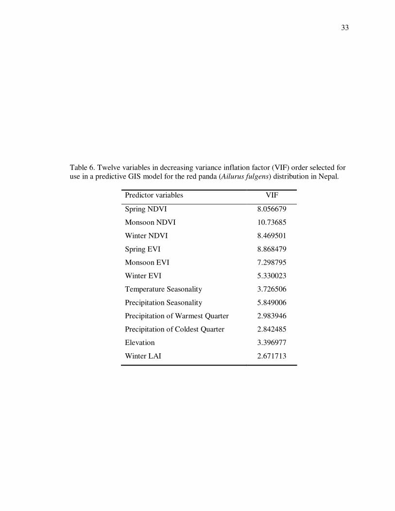
6. Twelve variables in decreasing variance inflation factor (VIF) order selected
for use in a predictive GIS model for the red panda (Ailurus fulgens)
distribution in Nepal ................................................................................................33
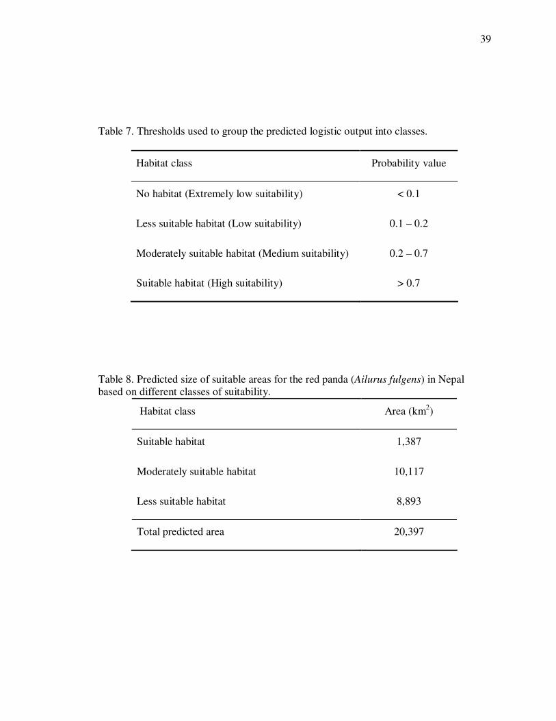
7. Thresholds used to group the predicted logistic output into classes.............................39
8. Predicted size of suitable areas for the red panda (Ailurus fulgens) in Nepal
based on different classes of suitability ....................................................................39
9. Relative percent contribution of 10 environmental variables (layers) to the red
panda (Ailurus fulgens) distribution in Nepal ...........................................................45
10. Size and percent of predicted red panda (Ailurus fulgens) habitat under
protected areas based on habitat classes ...................................................................57
11. Percents of red panda (Ailurus fulgens) suitable habitat, protected habitat and
human population change with size and number of protected areas in 5 regions
of Nepal.. .................................................................................................................59
12. Proportion of potential suitable habitat for the red panda (Ailurus fulgens
throughout Asia. ......................................................................................................63
13. Proportion of predicted red panda (Ailurus fulgens) habitat in Asian countries. ........63
ix
LIST OF FIGURES
Figure Page
1. Relative location of Nepal within southern Asia...........................................................9
2. Regional and administrative boundaries of Nepal.......................................................10
3. Distribution of protected areas in Nepal .....................................................................11
4. Locations of red panda (Ailurus fulgens) occurrences used in this study for
distribution modeling in Nepal.................................................................................14
5. Predicted logistic probability for red panda (Ailurus fulgens) occurrence in
Nepal .......................................................................................................................35
6. Omission rate at various logistic thresholds for the red panda (Ailurus fulgens)
occurrence test points...............................................................................................37
7. Predicted probability value for red panda (Ailurus fulgens) occurrence points. ...........38
8. Predicted potential suitable habitat for the red panda (Ailurus fulgens) in Nepal
(with regional boundaries included) .........................................................................40
9. Predicted potential suitable habitat at 0.5 threshold for red panda (Ailurus
fulgens) in Nepal (with regional boundaries included)..............................................41
10. Predicted potential suitable habitat for the red panda (Ailurus fulgens) in
Nepal (with political district boundaries depicted)....................................................42
11. Predicted potential suitable habitat at a 0.5 threshold for the red panda
(Ailurus fulgens) in Nepal (with political district boundaries depicted).....................43
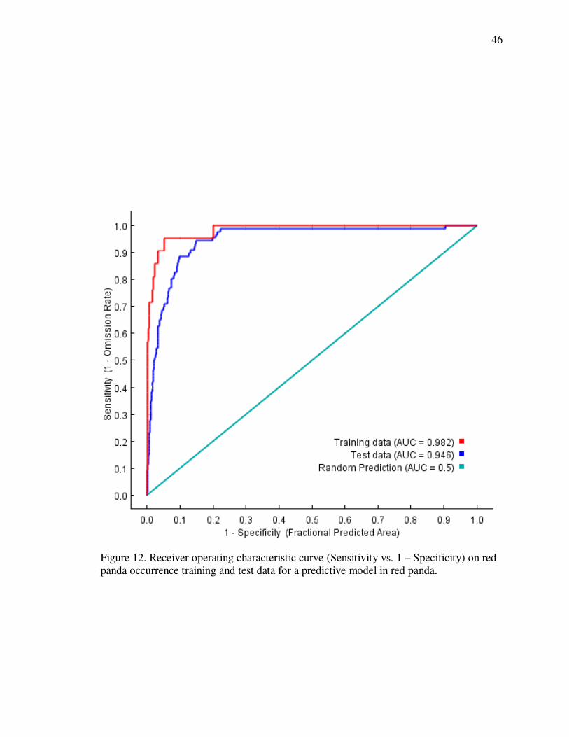
12. Receiver operating characteristic curve (Sensitivity vs. 1 – Specificity) on red
panda occurrence training and test data for a predictive model in red panda. ............46
13. Result of jackknife test for relative importance of environmental variables
using area under the curve (AUC) on test data for predictive GIS model for
the red panda (Ailurus fulgens) distribution in Nepal................................................47
14. Response of the red panda (Ailurus fulgens) presence to elevation (in meters) .........49
15. Response of the red panda (Ailurus fulgens) presence to tree cover ..........................50

x
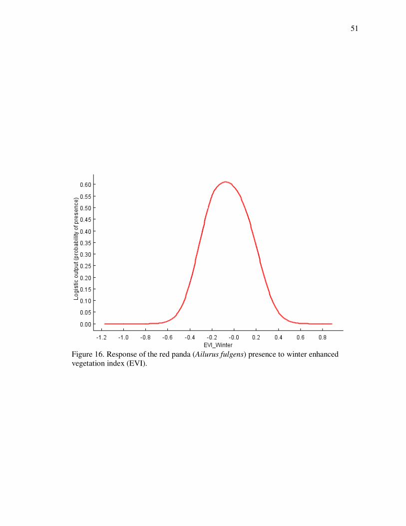
16. Response of the red panda (Ailurus fulgens) presence to winter enhanced
vegetation index (EVI).............................................................................................51
17. Response of the red panda (Ailurus fulgens) presence to land cover .........................52
18. Response of the red panda (Ailurus fulgens) presence to winter leaf-area
index (LAI)..............................................................................................................53
19. Response of the red panda (Ailurus fulgens) presence to precipitation (in mm)
in the coldest quarter................................................................................................54
20. Response of the red panda (Ailurus fulgens) presence to precipitation (in mm)
in warmest quarter ...................................................................................................55
21. Response of the red panda (Ailurus fulgens) presence to spring normalized
differential vegetation index (NDVI) .......................................................................56
22. Predicted potential suitable habitat for the red panda (Ailurus fulgens) within
protected areas in Nepal...........................................................................................60
23. Predicted potential suitable habitat at 0.5 threshold within protected areas for
the red panda (Ailurus fulgens) in Nepal ..................................................................61
24. Predicted potential suitable habitat for the red panda (Ailurus fulgens) in Asia.........64
25. Predicted potential suitable habitat at 0.5 threshold for the red panda (Ailurus
fulgens) in Asia........................................................................................................65

xi
ACRONYMS
ASCII American Standard Code for Information Interchange
AUC Area under Curve
CA Conservation Area
CITES Convention on International Trade on Endangered Species
CSV Comma separated value
DEM Digital Elevation Model
ESRI Earth System Resource Institute
EVI Enhanced Vegetation Index
FAO Food and Agriculture Organization
GAM Generalized Additive Model
GARP Genetic Algorithm for Rule Set Production
GIS Geographic Information System
GLCNMO Global Land Cover by National Mapping Organizations
GLM Generalized Linear Model
GPS Global Positioning System
ISCGM International Steering Committee for Global Mapping
IUCN International Union for Conservation of Nature and Natural
Resources (The World Conservation Union)
km kilometer
LAI Leaf-area Index
LPT Lowest Presence Threshold
MaxEnt Maximum Entropy
mm millimeter
MODIS Moderate Resolution Imaging Spectroradiometer
NDVI Normalized Difference Vegetation Index

xii
NIR Reflectance in near infra-red band
NP National Park
ROC Receiver Operator Curve
RPN Red Panda Network, Nepal
RS Remote Sensing
SPSS Statistical Package for Social Survey
SRTM Shuttle Radar Topography Mission
TXSTATE Texas State University-San Marcos
VIF Variance Inflation Factor
VIS Reflectance in visible band
xiii
ABSTRACT
DISTRIBUTION OF THE RED PANDA AILURUS FULGENS (CUVIER, 1825) IN
NEPAL BASED ON A PREDICTIVE MODEL
by
Naveen Kumar Mahato, B.Sc.
Texas State University-San Marcos
August, 2010
SUPERVISING PROFESSOR: MICHAEL R. J. FORSTNER
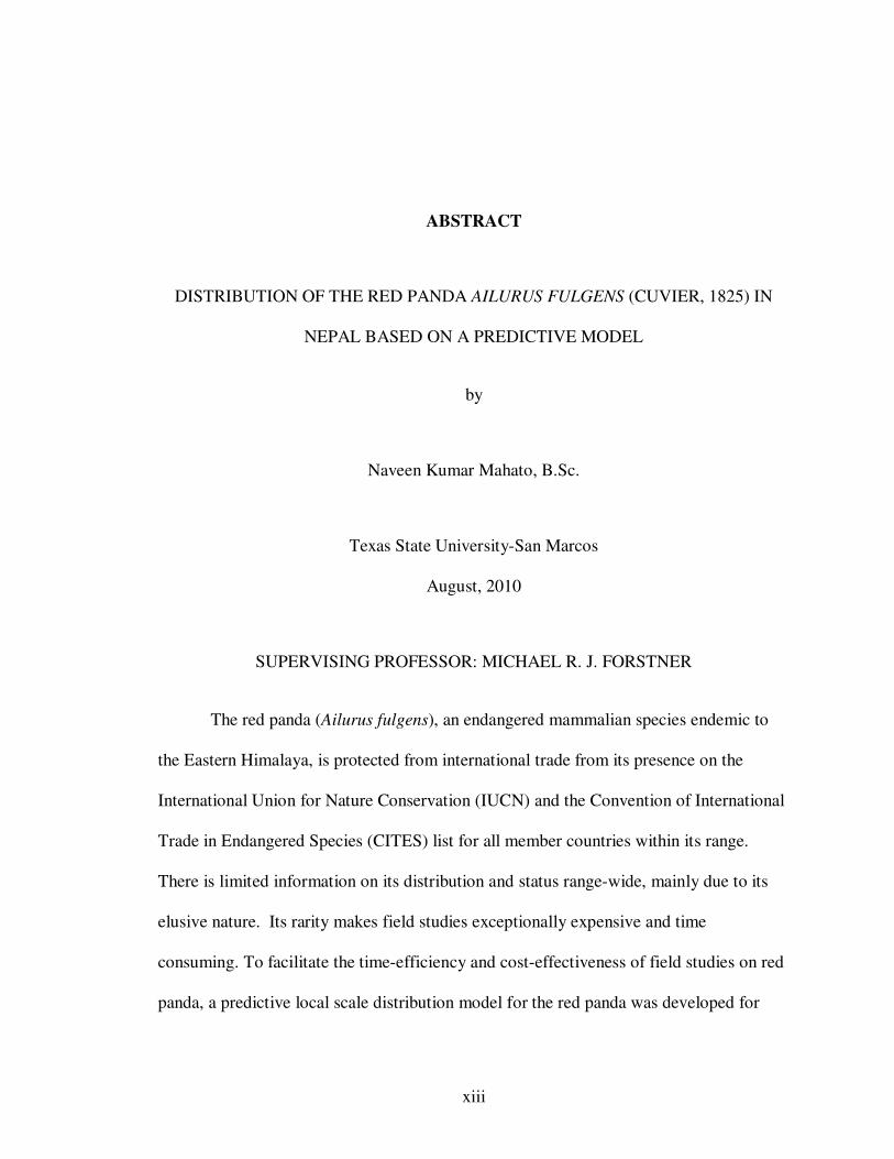
The red panda (Ailurus fulgens), an endangered mammalian species endemic to
the Eastern Himalaya, is protected from international trade from its presence on the
International Union for Nature Conservation (IUCN) and the Convention of International
Trade in Endangered Species (CITES) list for all member countries within its range.
There is limited information on its distribution and status range-wide, mainly due to its
elusive nature. Its rarity makes field studies exceptionally expensive and time
consuming. To facilitate the time-efficiency and cost-effectiveness of field studies on red
panda, a predictive local scale distribution model for the red panda was developed for
xiv
Nepal using maximum entropy (Maxent) species distribution modeling. In this method,
20 presence-only red panda occurrence points were used to train the model that used 10
uncorrelated environmental layers from various sources. A set of 86 independent points
of red panda occurrences was used to evaluate the validity of the model. A probabilistic
prediction for the red panda distribution was produced with a low omission rate and high
accuracy (test AUC = 0.946). Elevation and temperature seasonality followed by tree
cover were the most important environmental variables contributing to the red panda
distribution model. The estimated suitable habitat for red panda in Nepal based on a 0.1
threshold of presence were areas of approximately 20,400 km2. In Nepal 22.5 % of
suitable habitat falls in nine montane protected areas. Regional classification of habitat
demonstrated a larger proportion of suitable areas for red pandas occurred in the Eastern
Region of Nepal which also had high probability areas for red pandas and one of the
highest human population growth rates in Nepal. Amplification of the model to the global
scale predicted about 425,700 km2 of suitable areas for red pandas in six countries. The
current Maxent model overestimated the modern distribution of the red panda in Asia.
Despite the overestimation, this model can be used as an effective tool in planning future
studies of the species and conservation efforts.

1
INTRODUCTION
Statement of Problem
The red panda (Ailurus fulgens, Cuvier 1825) is a rare species listed as
“Vulnerable” in the International Union for Conservation of Nature (IUCN) Red List
(IUCN 2010). It is protected against international trade by inclusion in the Convention on
International Trade on Endangered Species (CITES) Appendix I. The red panda also has
legal protection in all countries within its range across a network of protected areas
(Choudhary 2001, Glatston 1994, Wei et al. 1999, Yonzon et al. 1997). However,
whether these legal protections and the existing network of protected areas are enough to
accommodate viable populations of red pandas remains a matter of debate. As with many
other endangered species, habitat fragmentation following deforestation has been a major
cause of population decline. This is evident, for example, in Langtang National Park in
Nepal, where red pandas are now sub-divided into four sub-populations or
metapopulation fragments (Yonzon and Hunter 1991). Such habitat fragmentation may
lead to inbreeding and a consequent loss of genetic variation. It may also cause other
effects, such as starvation in the giant panda, Ailuropoda melanoleuca, when fragments
of habitat experience widespread senescence and decline of forage (Reid et al. 1991).
2
Other forms of anthropogenic impacts, such as livestock grazing in red panda
habitat or simply the presence of herders and their dogs are additional sources of
disturbances to red pandas (Mahato 2004b, Pradhan et al. 2001, Yonzon and Hunter
1991). During the mid 20th
century, the demand for live harvest of red pandas from the
wild for display in western zoos was an important cause of the decline of wild
populations (Glatston 1994). Despite a lack of any real market value, red pandas are
hunted locally for the pelt and for sport in some areas (Choudhary 2001, Glatston 1994,
Wei et al. 1999, Yonzon et al. 1997).
The most pressing conservation problem for red pandas remains inadequate
information regarding ecology and distribution. Its status in the wild is not sufficiently
known nor its ecology documented. The extent of suitable habitat is also poorly
understood, which has hindered the planning of protected areas and habitat connectivity.
Background Information on Red Panda
The red panda has interested scientists, in part, because of the ambiguity of its
phylogenetic assignment. Classical systematists suggest the red panda along with the
giant panda, should be placed in the sub-family Ailurinae within the family Procyonidae,
instead of the sub-family Procyoninae which includes the New World procyonids
(Walker 1968). However, serological (Leone and Wiens 1956) and DNA hybridization
(O’Brien et al. 1985) studies alternatively suggested a closer relationship to the giant
panda of the bear family (Ursidae). While the results of DNA hybridization support
subsuming the red panda as a procyonid (Wayne et al. 1989), it was argued that
placement of the red panda in the family Procyonidae was based on superficial

3
similarities between the red panda and raccoons, such as face mask, ringed tails, etc. This
argument was based on anatomical features (Decker and Wozencraft 1991) and
cytogenesis (Wurster and Benirschke 1968), which suggested the red panda was a closer
relative to bears. Based on these debates of its phylogeny and as suggested by Eisenberg
(1981), placement of the red panda in a separate family – Ailuridae is currently widely
accepted (Glatston 1994).
The red panda is endemic to the eastern Himalayan broad-leafed and coniferous
forests (Olsen and Dinerstein 1998) extending from Nepal through India, Bhutan, China
and Myanmar. The red panda distribution extends from Namlung Valley (Mugu District)
and Rara Lake region in western Nepal eastward to the Min Valley in Western Sichuan
(Glatston 1994, Roberts and Gittleman 1984). Two subspecies of red panda are known –
Ailurus fulgens fulgens and A. f. styani. The later found in Myanmar and China is also
known as Styan’s or the Chinese red panda. The subspecies, A. f. fulgens, occurs in
Nepal, India, Bhutan and certain parts of China (Glatston 1994). However, the actual
distribution and isolation between these subspecies (if any) remain poorly understood.
The red panda inhabits fir-jhapra forests (fir with ringle bamboo in the
understory) with an altitudinal preference between 2,400 and 3,900 m (Pradhan et al.
2001, Yonzon and Hunter 1991). In China red pandas share habitat with giant pandas
(Wei et al. 2000). Despite the placement of red panda within the order Carnivora, it has a
specialized herbivore diet. The major proportion (54-100%) of its food consists of leaves
and shoots of bamboo (Arundinaria maling and Arundinaria aristata) followed by berries
of Sorbus microphylla and Sorbus cuspidata (Yonzon and Hunter 1991). Behaviorally,
the red panda is nocturnal and crepuscular (Roberts and Gittleman 1984). It is solitary

4
outside the mating season, but females are seen with their cubs between parturition and
the subsequent mating season (Pradhan et al. 2001, Yonzon and Hunter 1991). Red
pandas are largely sedentary and have a small home range between 1.38 and 11.57 km2.
Females have a smaller home range (mean = 2.37 km2) than males (mean = 5.12 km
2)
(Yonzon 1989). Because of specialized feeding behavior and narrow and specialized
habitat needs, the red panda is considered a habitat specialist.
Little was known about the ecology, status and distribution of this species in the
wild until the late 1980s (e.g., Johnson et al. 1988, Yonzon 1989). Prior to this period
most of the behavioral information on red pandas was from captive populations (e.g.,
Roberts 1981, Warnell 1988). A study in Langtang National Park in Nepal (Yonzon
1989) produced important information about habitat, feeding behavior, home range and
habitat preference. Another long-term study in Singhalila National Park in India (Pradhan
et al. 2001) provided additional ecological information. Some preliminary data came
from Wolong Reserve in China (Johnson et al. 1988, Reid et al. 1991). Recent studies in
Yele Nature Reserve (Wei et al. 2000) and Fengtongzhai Nature Reserve in China (Zhang
et al. 2004) produced important information on microhabitat selection and separation
between red and giant pandas. Recent surveys in Kanchenjunga Conservation Area
(Mahato 2004a), Sagarmatha (Everest) National Park (Mahato 2004b), Ilam and
Panchthar districts (RPN 2006-2009) supplied field-based confirmation of red panda
occurrences. Red pandas were also reported in Sichuan and Yunnan provinces and Tibet
in China (Wei et al. 1999), in Sikkim, Darjeeling District in West Bengal, and the
northern part of Arunachal Pradhesh in India (Choudhary 2001).

5
Various techniques for modeling the distribution of species have been developed
in recent years (Guisan and Thuiller 2005), and Geographic Information Systems (GIS)
became a vital tool in this regard. In analyzing multivariate environments, GIS facilitates
an understanding of the relation of environmental variables to species presence. This tool
in combination with remotely sensed data has been successfully used to predict species
distributions, e.g., wolf, Canis lupus (Corsi et al. 1999) and Asiatic black bear, Ursus
thibetanus japonicus and Japanese serow, Naemorhedus crispus (Doko 2007). Species
distribution models have been used to guide field survey efforts to successfully find
populations (Guisan et al. 2006), support species conservation prioritization and reserve
selection (Leathwick et al. 2005), predict species invasion (Thuiller et al. 2005),
delimitation of species, and guide the reintroduction of endangered species (Pearce and
Lindenmayer 1998).
Rationale of the Study
Understanding the spatial occurrence of a species is one of the first steps for its
preservation or management. The most pressing problem in the conservation of the red
panda is insufficient information regarding occurrence (Glatston 1994, Yonzon et al.
1997). Like all endangered or rare species, gathering such information for such an elusive
species is both time and resource consuming. Therefore, predicting a species distribution
is an important component of a conservation plan (Pearson 2007). Predicting distribution
becomes more important for elusive species like the red panda for two reasons – firstly,
detection is limited by its rarity and small body size, and secondly, limited accessibility to
remote and rugged habitat makes field surveys exceptionally time consuming, expensive,
and difficult, consequently hindering conservation efforts. Thus, modeling tools, which

6
identify the environmental variables related to a species occurrence, have been developed
to overcome these problems in conservation planning (Pearson 2007). In this effort,
association among environmental variables and species occurrence are identified and
environmental variables suitable for the species are extrapolated spatially across the area
of concern.
Solving the issue of the red panda’s status in the wild will require complementary
investigations based on field studies combined with GIS. For example, Yonzon and
Hunter (1991) suggested a population of 37 adult red pandas inhabited Langtang National
Park, which provided 108 km2 of suitable habitat for red pandas (ecological density = 1
panda per 2.9 km2). Pradhan et al. (2001) indicated an estimated crude density of 1 panda
per 1.67 km2 existed in Singhalila National Park. A GIS based study (overlaying altitude
– 3,000-4,000 m, forest cover – Fir-jhapra forest, and rainfall > 2,000 mm) using the
ecological density observed in the Langtang National Park produced a population
estimate of 314 red pandas in 912 km2 of potential habitat in the Nepal Himalaya
(Yonzon et al. 1997). This might have been either an overestimation or underestimation
of habitat for two reasons – recent spatial data and the relationship between red panda
occurrence and other environmental variables were not used in the study. Field studies in
Wolong Reserve in China (Johnson et al. 1988, Reid et al. 1991) did not provide enough
information regarding the abundance of red pandas. Therefore, I will use recent satellite
data to estimate the present extent of red panda habitat and analyze the correlation
between environmental variables and species occurrence, hence providing baseline
information for planning habitat connectivity and a design for protected areas.

7
OBJECTIVES
The goals of my study were to understand and predict the red panda distribution
by assessing the relationship between presence of the species and various environmental
parameters. The specific objectives were:
1. To develop a landscape-level model for the red panda distribution for Nepal,
2. To use GIS analysis to test for correlations between the occurrence of red pandas
and available ecological components (environmental factors) of habitat, and
3. To assess the conservation status of the red panda in Nepal based on the
developed model.

8
STUDY AREA
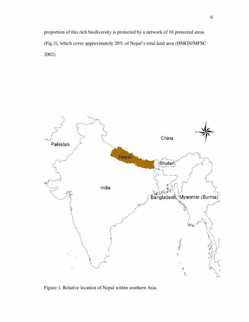
Nepal lies between latitudes 26° 22′ and 30° 27′ N and longitudes 80° 04′ and 88°
12′ E between India and China in southern Asia (Fig.1). China is north of Nepal, while
India encompasses the remaining border with Nepal. Nepal, with an area of 147,181 km2,
is divided into five development regions and 75 districts (Fig.2). The development
regions of Nepal from east to west are: Eastern, Central, Western, Mid-western and Far-
western.
Nepal is predominantly a mountainous country with an increasing elevational
gradient from south to north. The elevational gradient changes from 63 m above sea level
in the southern plains to 8,848 m on the top of the Mount Everest within an average
north-south lateral distance of 150 km and causes variation in climatic conditions. In the
southern area, there is a narrow belt of lowlands with a tropical climate. Smaller hills
with a sub-tropical climate to the north supplant the lowlands and further north the
mountains with a temperate climate replace the hills. The high mountains with sub-alpine
and alpine environments occur in the northern part of the country.
The variation in the elevation gradient and the resulting varied bioclimatic
circumstances support a highly diverse flora and fauna. Nepal is located at a transition of
the Pale-arctic and Indomalayan biogeographic realms (Udvardy 1975). A combination
of the flora and fauna of both realms contributes to the rich biodiversity of the country. A
9
proportion of this rich biodiversity is protected by a network of 16 protected areas
(Fig.3), which cover approximately 20% of Nepal’s total land area (HMGN/MFSC
2002).
Figure 1. Relative location of Nepal within southern Asia.

Figure 2. Regional and administrative boundaries of Nepal.
10

Figure 3. Distribution of protected areas in Nepal.
11
12
MATERIALS AND METHODS
Three components compose the statistical model of a species distribution – an
ecological component (environmental variables), the presence dataset, and a predictive
algorithm (statistical/ modeling tool) (Austin 2002).
Red Panda Occurrence Data
Species occurrence data is usually in two forms – presence and absence. Presence
data are easy to obtain compared to the absence data. While use of both presence and
absence data improve the performance of a model (Brotons et al. 2004), absence data are
usually unavailable or may be unreliable in many cases, especially for rare and elusive
species. This can lead to a false absence, which may become a serious bias in a
distribution model (Hirzel et al. 2002). While locations with obvious red panda absence,
e.g. the lowlands and higher elevations beyond red panda known range, can provide
absence data, these were not used as well. Therefore, in this study only presence data
were used.
Occurrence points for red pandas were based on presence data obtained from
previous surveys. These data came from six areas occupied by red pandas in Nepal.
These locations are listed in Table 1 and mapped in Figure 4. Though there were
variations in how the different surveys were conducted, occurrence points were based on
direct or indirect evidence with the location recorded using a handheld GPS unit. Most

13
locations were based on indirect evidence of red panda presence, in most cases
confirmation was based on fecal droppings.
More than 600 occurrence points in six habitat fragments were available.
However, my analysis was at a resolution of 1 km; therefore, there were multiple points
per pixel. I removed the multiple points per pixel in ArcMap 9.3 (ESRI Inc., Redlands
CA) using Hawth’s analysis tool (www.spatialecology.com). After correcting for
multiple points per pixel, I obtained 107 unique points in each pixel.
Table 1. Red panda (Ailurus fulgens) presence points used in predictive GIS model.
Locations Source
Dhorpatan Hunting Reserve Sharma and Kandel (2009)
Kanchenjunga CA Mahato (2004a)
Ilam and Panchthar districts RPN (unpublished data)
Sagarmatha NP (Bufferzone) Mahato (2004b)
Langtang NP Stephens (2003), Regmi (2009)
Manang district Stephens (2003)
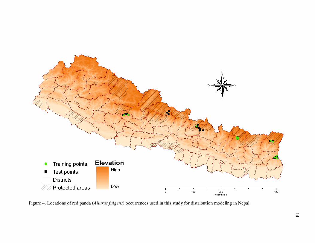
Figure 4. Locations of red panda (Ailurus fulgens) occurrences used in this study for distribution modeling in Nepal.
14

15
Environmental layers
Knowledge of the ecology of a species is helpful in deciding which biologically
relevant environmental variables to use in distribution modeling. I collected and reviewed
the available literature on red pandas and combined this information with my
observations in the field in understanding the environmental variables potentially
influencing the distribution of red pandas. I created spatial layers of the environmental
variables at the landscape level and used ArcMap to sort the spatial layers. The
environmental variables used in the model are listed in Table 1.
Table 2. Environmental layers used in modeling the distribution of red pandas (Ailurus
fulgens) in Nepal.
Data layers Sources
19 Bioclimatic layers World Clim
Normalized difference vegetation index (NDVI) Satellite data (3 seasons data)
Enhanced vegetation index (EVI) Satellite data (3 seasons data)
Leaf area index (LAI) Satellite data (3 seasons data)
Land cover
Tree percent cover Derived from satellite data
Altitude World Clim
16
Bioclimatic Layers
Bioclimatic variables were downloaded as layers in ESRI grids format from free
domain public global climate data – WorldClim (Hijmans et al. 2005). The bioclimatic
layers were derivatives from monthly precipitation (mm) and temperature (Celsius) data.
An additional 19 biologically meaningful variables were generated from these data
(Table 3) representing annual trends (mean annual temperature and precipitation),
seasonality (e.g., annual range in temperate and precipitation), and limiting
environmental factors (e.g., temperate and precipitation of a certain quarter) (Hijmans et
al. 2005). These climatic layers were generated through interpolation of average monthly
climate data of 50 years from more than 47,000 weather stations throughout the world
(e.g., Global Historical Climatology Network - GHCN, the Food and Agriculture
Organization – FAO, International Center for Tropical Agriculture – CIAT, World
Meteorological Organization – WMO, R-HYdronet).
Bioclimatic layers were available at a resolution of 30 arc sec which is
approximately 1 km pixel size. The layers were masked from the global dataset in
geographic coordinate system (WGS84) for the study area.
Elevation
The elevation layer was obtained in ESRI grids format from WorldClim which
was generated from the Shuttle Radar Topography Mission (SRTM) elevation database.
This layer was in the same spatial resolution as the bioclimatic layers (30 seconds arc)
and the geographic coordinate system (WGS84).

17
Table 3. Nineteen bioclimatic layers obtained from WorldClim for use in a predictive
GIS model for the red panda (Ailurus fulgens) in Nepal.
Environmental layers Type
Annual Mean Temperature – P1 Continuous
Mean Diurnal Range – P2
(Mean of monthly (max temp - min temp) ) Continuous
Isothermality [(P2/P7) ××××100 ] – P3 Continuous
Temperature Seasonality (standard deviation ××××100) – P4 Continuous
Max Temperature of Warmest Month – P5 Continuous
Min Temperature of Coldest Month – P6 Continuous
Temperature Annual Range (P5 – P6) – P7 Continuous
Mean Temperature of Wettest Quarter – P8 Continuous
Mean Temperature of Driest Quarter – P9 Continuous
Mean Temperature of Warmest Quarter – P10 Continuous
Mean Temperature of Coldest Quarter – P11 Continuous
Annual Precipitation – P12 Continuous
Precipitation of Wettest Month – P13 Continuous
Precipitation of Driest Month – P14 Continuous
Precipitation Seasonality (Coefficient of Variation) – P15 Continuous
Precipitation of Wettest Quarter – P16 Continuous
Precipitation of Driest Quarter – P17 Continuous
Precipitation of Warmest Quarter – P18 Continuous
Precipitation of Coldest Quarter – P19 Continuous

18
Satellite-derived Vegetation Indices
Three types of vegetation indices, normalized differential vegetation index
(NDVI), enhanced vegetation index (EVI) and leaf-area index (LAI) derived from
satellite data, were used as predictors of the red panda distribution. All three indices were
obtained from MODIS (Moderate Resolution Imaging Spectroradiometer) Terra sensor.
These MODIS products were obtained from Land Processes Distributed Active Archive
Center (LPDAAC) located at U. S. Geological Survey (USGS) Earth Resources
Observation and Science (EROS) Center (http://lpdaac.usgs.gov) in HDF-EOS data
format (.hdf file format). NDVI and EVI were obtained as a 16-day mosaic at a spatial
resolution of 1 km, while LAI was obtained as an eight-day mosaic at the same spatial
resolution, all three in Sinusoidal projection system (LPDAAC 2008).
The vegetation indices obtained from various seasons were used to incorporate
the seasonal variation in vegetation. For the purpose of this study, the annual cycle was
arbitrarily divided into three seasons: pre-monsoon (January – June), monsoon (June –
September) and post-monsoon (September – December). The products used in this study
(based on the best available products) are listed in Table 4.
19
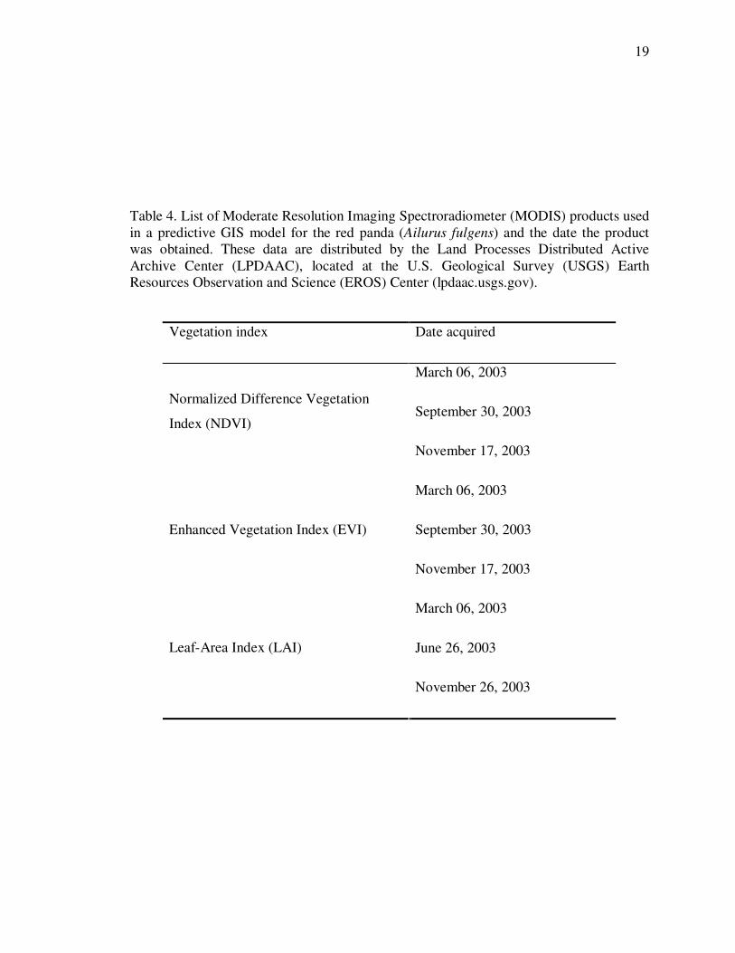
Table 4. List of Moderate Resolution Imaging Spectroradiometer (MODIS) products used
in a predictive GIS model for the red panda (Ailurus fulgens) and the date the product
was obtained. These data are distributed by the Land Processes Distributed Active
Archive Center (LPDAAC), located at the U.S. Geological Survey (USGS) Earth
Resources Observation and Science (EROS) Center (lpdaac.usgs.gov).
Vegetation index Date acquired
March 06, 2003
September 30, 2003 Normalized Difference Vegetation
Index (NDVI)
November 17, 2003
March 06, 2003
September 30, 2003 Enhanced Vegetation Index (EVI)
November 17, 2003
March 06, 2003
June 26, 2003 Leaf-Area Index (LAI)
November 26, 2003
20
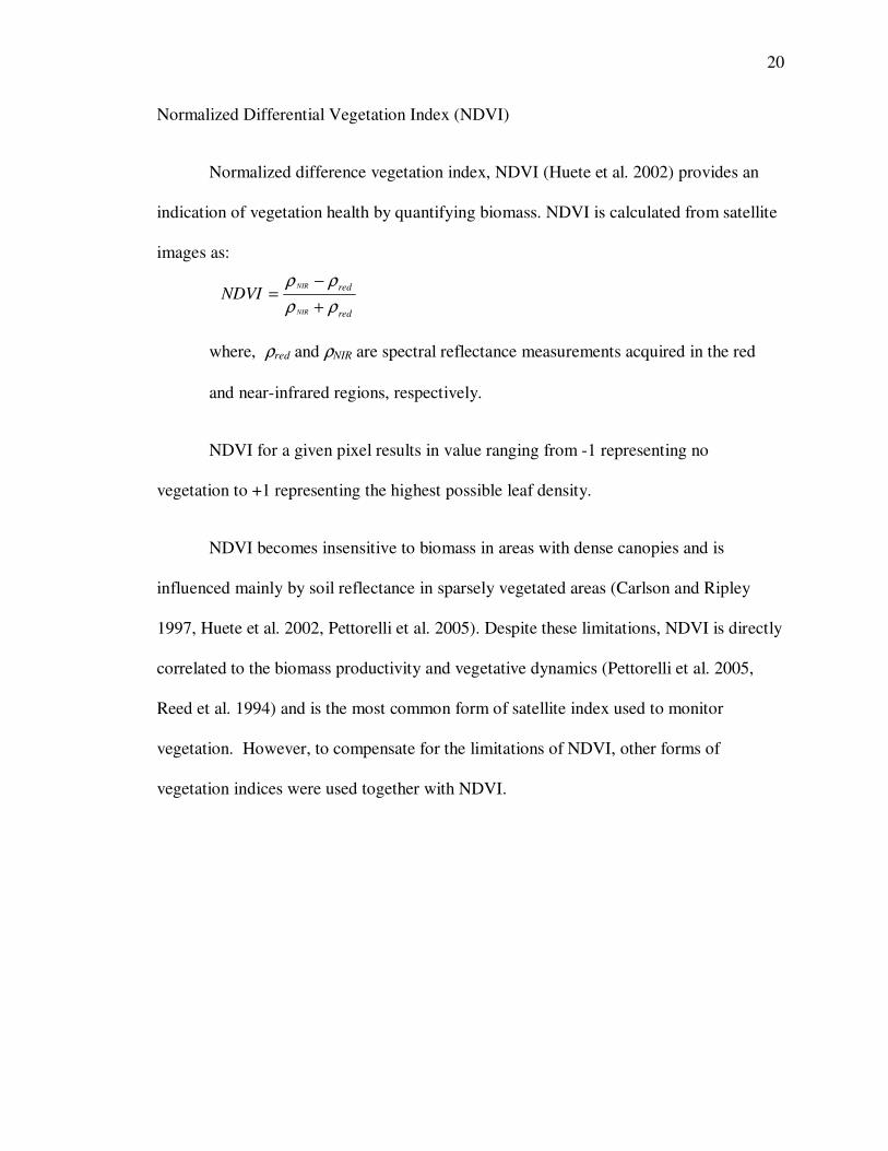
Normalized Differential Vegetation Index (NDVI)
Normalized difference vegetation index, NDVI (Huete et al. 2002) provides an
indication of vegetation health by quantifying biomass. NDVI is calculated from satellite
images as:
where, ρred and ρNIR are spectral reflectance measurements acquired in the red
and near-infrared regions, respectively.
NDVI for a given pixel results in value ranging from -1 representing no
vegetation to +1 representing the highest possible leaf density.
NDVI becomes insensitive to biomass in areas with dense canopies and is
influenced mainly by soil reflectance in sparsely vegetated areas (Carlson and Ripley
1997, Huete et al. 2002, Pettorelli et al. 2005). Despite these limitations, NDVI is directly
correlated to the biomass productivity and vegetative dynamics (Pettorelli et al. 2005,
Reed et al. 1994) and is the most common form of satellite index used to monitor
vegetation. However, to compensate for the limitations of NDVI, other forms of
vegetation indices were used together with NDVI.
red
red
NIR
NIR
NDVIρρ
ρρ
+
−=
21
Enhanced Vegetation Index (EVI)
Enhanced vegetation index, EVI (Huete et al. 2002) is an improved form of
vegetation index which provides complementary information about variation in
vegetation minimizing the insensitivity of NDVI to dense canopy and the residual
influence of atmospheric aerosols (Huete et al. 2002, Pettorelli et al. 2005). The
adjustment factor used in EVI makes it sensitive to topography (Matsushita et al. 2007).
EVI is calculated from satellite images as:
where, ρred, ρNIR and ρblue are spectral reflectance measurements acquired in the
red, near-infrared and blue regions, respectively; L (= 1) is canopy background
adjustment, G (= 2.5) is gain factor, C1 (= 6) and C2 (= 7.5) are coefficient of
aerosol resistance.
Leaf-Area Index (LAI)
Leaf-area index, LAI (sometimes also known as plant-area index – PAI) is the
total area of leaves per unit area of the ground (Curran and Steven 1983) and indicates an
index of canopy density.
Land Cover
Land cover data were obtained from Global V.1 of the Global Land Cover by
National Mapping Organizations (GLCNMO) from the Secretariat of International
Steering Committee for Global Mapping (ISCGM). GLCNMO was created by using a
LCCGEVI
bluered
red
NIR
NIR
+×−×+
−=
ρρρ
ρρ
21
22
16-day composite of MODIS data (Terra Satellite) acquired in 2003. These data are
available at a resolution of 30 arc sec (~ 1 km) and has 20 land cover classes (Table 5) at
a global scale based on the land cover classification system developed by the Food and
Agriculture Organization (FAO). However, four land cover classes did not occur in
Nepal; resulting in only 16 classes. The land cover map was obtained in geographic
coordinate system WGS84.
Tree Cover
Tree cover data were also obtained from a global version of a vegetation /percent
tree cover map produced by ISCGM. The tree cover data were derived from a 16-day
composite MODIS (Terra Satellite) image acquired in 2003 at a resolution of 30 arc sec
(~ 1 km). The global percent tree cover represents the density of trees on the ground. The
percent tree cover was derived from the most photosynthetic period of the year to account
for leaf drop from deciduous trees during dry seasons.
Percent tree cover ranges from 0 to 100 % cover. However, the 8-bit raster layer
may contain value between 0 and 255. Therefore, pixel value in this layer ranges between
0 and 100 for tree cover, and 255 for the pixels with “no-data”. The percent tree cover
map was obtained in geographic coordinate system WGS84.
Multicolinearity Analysis Between Environmental Layers
Intercorrelation among environmental predictors may cause a bias, such as
multicollinearity, in prediction (Graham 2003). Multicollinearity occurs primarily when
predictor variables are more significantly correlated with each other than they are with a

23
Table 5. Sixteen coded land cover classes used in a predictive GIS model for the red
panda (Ailurus fulgens) distribution in Nepal. Land cover classes coded 9, 14, 15 and 19
do not occur in Nepal at 1 km2 pixel size.
Code Land cover class
1 Broadleaf evergreen forest
2 Broadleaf deciduous forest
3 Needle-leaf evergreen forest
4 Needle-leaf deciduous forest
5 Mixed forest
6 Tree open
7 Shrub
8 Herbaceous
10 Sparse vegetation
11 Cropland
12 Paddy field
13 Cropland / other vegetation mosaic
16 Bare area, consolidated (gravel, rock)
18 Urban
19 Snow / ice
20 Water bodies

24
dependent variable. Multicollinearity among predictors in statistical approaches to
species distribution modeling has been detected by using cross correlations (e.g., Kumar
and Stohlgren 2009), cross correlation in combination to other tools (e.g., Doko 2007),
and variance inflation factor (VIF) (e.g., Lai 2009, Negga 2007). In this study,
multicollinearity was examined by calculating VIF for each predictor.
VIR indicates inflation in the variance of each regression coefficient compared
with a situation of orthogonality. As a rule of thumb, predictors, those with a VIF > 10,
are considered under the influence of multicollinearity. A VIF was calculated as:
where R2 is a coefficient of determination.
I generated 200 random points throughout Nepal using Hawth’s analysis tool in
ArcMap and added these to the 107 red panda occurrence points to calculate a VIF. VIF
for all non-categorical environmental predictors was calculated against these 307 points
using the linear regression tool in the statistical software SPSS 18.0 (SPSS Inc., Chicago,
IL). The variable with the highest VIF was removed and a VIF for the remaining
variables was re-calculated. Removal of any one variable significantly changed the VIF
of the remaining variables; therefore, the process was reiterated until all the variables had
a VIF < 10.
All pre-selected variables excluding tree cover and land cover were subjected to
VIF analysis. Land cover was excluded from the VIF analysis because it is a categorical
(discrete) variable. Tree cover is an important variable in determining red panda
21
1
RVIF
−=
25
distribution; therefore, it was selected deliberately without testing for correlation with
other variables excluding it from the VIF analyses.
MaxEnt Distribution Modeling
A wide range of approaches is available for species distribution modeling which
uses both presence-only and presence-and-absence datasets. Common approaches include
the generalized linear model (GLM) and generalized additive model (GAM), which use
both presence and absence datasets (Guisan et al. 2002, Pearce and Ferrier 2000). Several
other approaches are available which involve ecological niche factor analysis (ENFA),
e.g., Genetic Algorithm for Rule-set Production – GARP (Stockwell and Peters 1999)
and Maximum Entropy – MaxEnt (Phillips et al. 2006). MaxEnt was used in this study
because of its better performance and availability of presence-only data.
Maximum Entropy is a general-purpose machine learning method in niche
modeling of species using presence-only data (Phillips et al. 2006). This approach uses
environmental (ecological) factors as constraints in estimating the probability of a species
distribution. Since presence-only points are the most common form of data available in
niche modeling, it is an advantage to have a framework based on presence-only data.
Predicting a species distribution in MaxEnt is accomplished using the software Maxent
version 3.2.1 (http://www.cs.princeton.edu/~schapire/maxent/).
Maxent modeling has been used to predict distribution of a wide range of species
(e.g., Asiatic black bear (Ursus thibetanus japonicus) and Japanese serow (Naemorhedus
crispus) (Doko 2007); freshwater diatoms (Didymosphenia geminate) (Kumar et al.
2009); Canacomyrica monticola (Kumar and Stohlgren 2009); various amphibian species
26
(Negga 2007); various geckos’ species (Pearson et al. 2007). While the advantage of
using the Maxent modeling over other techniques is explained by the use of presence-
only data; it also gives the best result (Kumar et al. 2009) and performs well with a small
number of presence data (Pearson et al. 2007, Kumar and Stohlgren 2009).
MaxEnt uses environmental factors in ASCII formats and the binary species
occurrence points in CSV file format. Two files with red panda occurrence points –
training file (20 points) and test file (87 points) were entered along with the ASCII
environmental layers. The user-specified parameters – regularized multiplier was set to 1,
convergence threshold was set to 10-5
, and maximum iterations were set to 500. In
addition to 21 presence points, additional 10,000 background points were used to
determine the MaxEnt distribution. As output, a logistic output format was selected. In
addition, response curves and jackknife test of variable importance were also selected.
Processing of Environmental Layers
MaxEnt requires all environmental layers to be in the same coordinate system and
spatial resolution and cover the same geographic extent. The environmental layers were
obtained from various sources in different coordinate systems and spatial resolutions
(pixel size). The layers were processed to a single coordinate system, pixel size and the
same geographic extent. Since most of the layers were in geographic coordinate system
WGS84 and had a spatial resolution of 1 km, all the other layers were re-projected to
geographic coordinate system WGS84 and re-sampled at a pixel size of 1 km. All layers
were masked with the boundary of Nepal to ensure the same geographic extent. Pre-

27
processing of spatial layers was carried out in ArcMap 9.3 and Imagine 9.2 (ERDAS Inc.,
Norcross, GA).
All pre-processed environmental layers were converted into ASCII file format
using ArcMap 9.3 for analysis. The presence points were imported in ArcMap and
processed in a shapefile format (.shp file). This layer was also re-projected into the same
coordinate system as the environmental layers. Then the red panda occurrence points
were exported into CSV table format. MaxEnt reads environmental layers in ASCII
format (.asc file extension) and occurrence points in CSV table format (.csv file).
Layer Reduction
After removal of auto-correlated predictor variables, the remaining 14 predictor
variables were initially used to run the model. Variables with the lowest contribution to
the model were removed in a step by step process until a significant loss in test AUC was
observed in the ROC curve. A goodness of fit analysis tested whether the final model
with the fewest variables differed from the model with all variables. The logistic
prediction values were classified into habitat suitability classes and 261 points were
generated randomly representing all classes. These points were used to run a goodness of
fit test between the two models
The sample error matrix (Story and Congalton 1986) was used to estimate the
agreement between the final model and the model with all 14 predictors. In the sample
error matrix, the proportion of sample pixel that falls in the same category in both models
provides an estimate of overall agreement between the two models.
28
Threshold of Presence
Following the recommendations of Liu et al. (2005) and Pearson (2007), four
thresholds of presence were considered that used presence-only species occurrence data.
1. A fixed threshold value was chosen based on careful observation of probability
value of all the presence points for the red panda (Manel et al. 1999, Robertson et
al. 2001). I also evaluated a commonly used threshold of 0.5 (Jimenez-Valverde
and Lobo 2007).
2. A fixed sensitivity (Pearson et al. 2004) of 90% was chosen which corresponded
to a 10% omission rate.
3. The lowest presence threshold (LPT) (Pearson et al. 2006, Philips et al. 2006) was
the lowest probability value at a known presence point of the red panda.
4. The threshold of presence was determined at the point where sensitivity and
specificity are equal (Pearson et al. 2004).
Model Evaluation
Testing or validation is required to assess the predictive performance of a
distribution model. A subset of randomly selected set of 86 points (80% of total presence
points) was split from the entire 107 red panda occurrence points to evaluate the model
(Fielding and Bell 1997). Both threshold-dependent and threshold-independent methods
were used in model evaluation. In the threshold-dependent method, model performance
was investigated using extrinsic omission rate (Phillips et al. 2006). The omission rate is
29
a fraction of test localities that fall into pixels not predicted as suitable for red pandas. In
the threshold-independent method, the model was evaluated using a ROC (receiver
operating characteristics) curve.
Receiver Operating Characteristics (ROC) Curve
A receiver operating characteristics (ROC) curve is a threshold independent
method widely used in evaluating species distribution models (Fielding and Bell 1997),
which relates to the relative proportion of correctly and incorrectly classified predictions
over a wide and continuous rage of threshold levels. A ROC is a graphical plot of
“sensitivity” and “1 – specificity” for all possible thresholds. Sensitivity is a measure of
the proportion of actual positives identified correctly, while specificity is a measure of the
proportion of negatives which are correctly identified.
ROC has proved to be highly correlated with other test statistics, e.g., Cohen’s
Kappa Coefficient (Cohen 1960), used in evaluating species distribution models (Manel
et al. 2001). Both presence and absence data are needed to calculate a ROC. However,
presence-only data are used in MaxEnt. In order to overcome this gap, MaxEnt has a
built-in function which uses random background points (pseudo-absence) against
presence points (Phillips et al. 2006). An area under the curve (AUC) value indicates the
efficacy of the model. AUC values ranges between 0 and 1. In the case of a random
prediction, the AUC value is 0.5.
30
Relative Importance of Environmental Variables
MaxEnt assesses the importance of variables to the distribution model. MaxEnt
keeps track of the contribution (gain) of each environmental variable to the model output.
The relative contribution of each variable is converted into a percent at the end of the
training process. However, the percent contributions are only heuristically defined, and
especially when there are highly correlated variables, they should be cautiously
interpreted.
MaxEnt assesses the relative importance of a predictor variable running jackknife
operations. Jackknife operates by sequentially excluding one variable at a time out of the
model and running a new model using the remaining variables. It then runs the model
using only the excluded variables in isolation.
Conservation Status of Red Panda in Nepal
The protected areas with predicted suitable red panda habitat were identified and
the extent of suitable habitat protected in the country was estimated by clipping the
predicted area by the protected area boundary. Considering the regions as a unit of
comparison, predicted red panda suitable areas were compared with human population
growth in the districts with predicted red panda habitat within the last three decades.
Red Panda Habitat Projection at Global Scale
The red panda suitability model derived for Nepal was used to project potential
suitable habitat for the red panda throughout its range. The projection was carried out at
the same resolution as the model (30 arc sec, i.e., approx. 1 km) and at the geographic

31
extent encompassed by north-east Pakistan, northern India, southern part of Mongolia,
the entire area of China, Nepal, Bhutan, Myanmar, Laos, Vietnam, Bangladesh, and part
of Taiwan and Thailand.

32
RESULTS
Multicolinearity Analysis between Environmental Layers
The intercorrelation analysis for 29 environmental predictor variables resulted in
17 layers that were highly correlated and were dropped stepwise. Only 12 layers were
obtained with a VIF value < 10 (Table 6).
Layer Reduction
The initial model used all 14 remaining variables, 12 after removing the
autocorrelated variables, tree cover and the land cover. The step by step removal of
predictor variables resulted in a final model with only 10 variables. Spring EVI, monsoon
NDVI, winter NDVI and monsoon EVI were removed respectively in each step based on
their minimal contributions to the model. Other variables made significant contributions
to the model, and therefore, were not removed.
My decision of selecting a model with only 10 predictor variables was based on
two factors. First, goodness of fit showed no significant deviation between the two
models (χ2 = 4.385, P = 0.223, df = 3). Second, the sample error matrix showed an
overall agreement between the two models of 88.12%.
33
Table 6. Twelve variables in decreasing variance inflation factor (VIF) order selected for
use in a predictive GIS model for the red panda (Ailurus fulgens) distribution in Nepal.
Predictor variables VIF
Spring NDVI 8.056679
Monsoon NDVI 10.73685
Winter NDVI 8.469501
Spring EVI 8.868479
Monsoon EVI 7.298795
Winter EVI 5.330023
Temperature Seasonality 3.726506
Precipitation Seasonality 5.849006
Precipitation of Warmest Quarter 2.983946
Precipitation of Coldest Quarter 2.842485
Elevation 3.396977
Winter LAI 2.671713
34
Red Panda Distribution Model
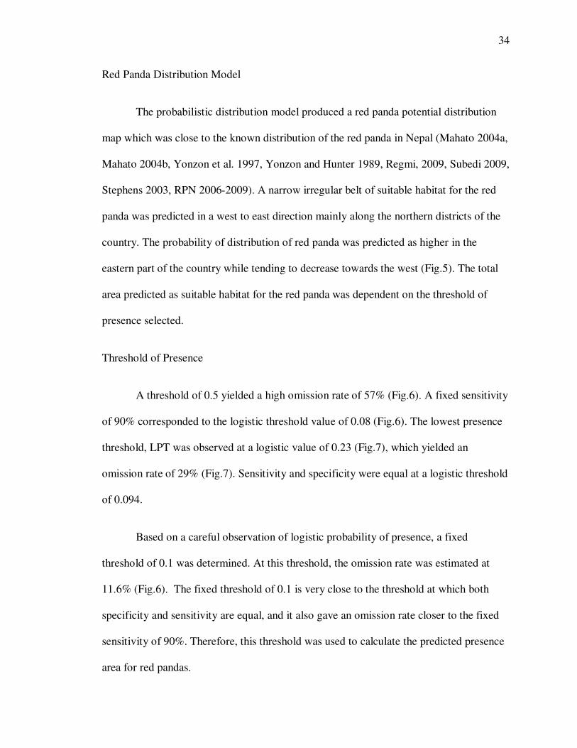
The probabilistic distribution model produced a red panda potential distribution
map which was close to the known distribution of the red panda in Nepal (Mahato 2004a,
Mahato 2004b, Yonzon et al. 1997, Yonzon and Hunter 1989, Regmi, 2009, Subedi 2009,
Stephens 2003, RPN 2006-2009). A narrow irregular belt of suitable habitat for the red
panda was predicted in a west to east direction mainly along the northern districts of the
country. The probability of distribution of red panda was predicted as higher in the
eastern part of the country while tending to decrease towards the west (Fig.5). The total
area predicted as suitable habitat for the red panda was dependent on the threshold of
presence selected.
Threshold of Presence
A threshold of 0.5 yielded a high omission rate of 57% (Fig.6). A fixed sensitivity
of 90% corresponded to the logistic threshold value of 0.08 (Fig.6). The lowest presence
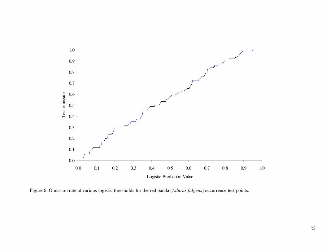
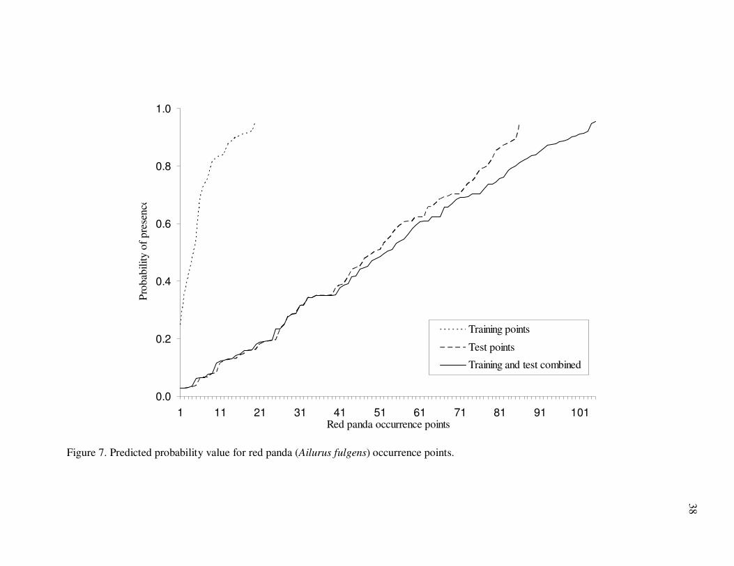
threshold, LPT was observed at a logistic value of 0.23 (Fig.7), which yielded an
omission rate of 29% (Fig.7). Sensitivity and specificity were equal at a logistic threshold
of 0.094.
Based on a careful observation of logistic probability of presence, a fixed
threshold of 0.1 was determined. At this threshold, the omission rate was estimated at
11.6% (Fig.6). The fixed threshold of 0.1 is very close to the threshold at which both
specificity and sensitivity are equal, and it also gave an omission rate closer to the fixed
sensitivity of 90%. Therefore, this threshold was used to calculate the predicted presence
area for red pandas.
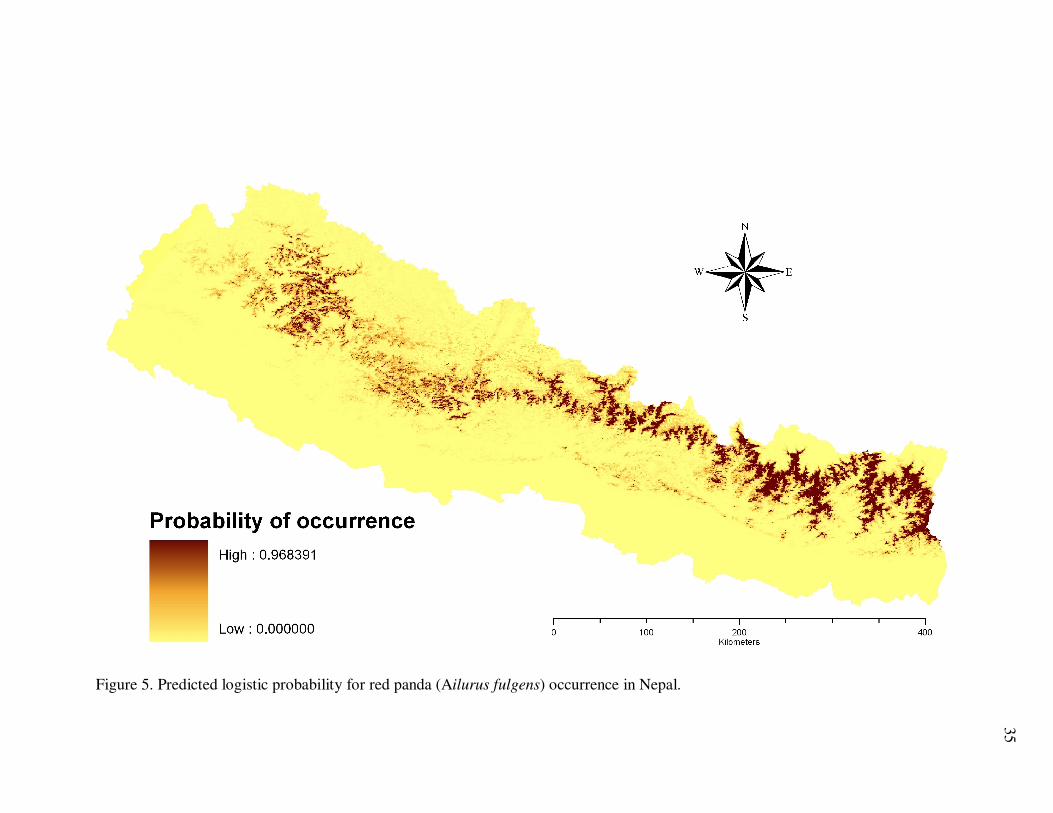
Figure 5. Predicted logistic probability for red panda (Ailurus fulgens) occurrence in Nepal.
35

36
Habitat Suitability Classes
After a threshold of red panda presence was determined, three arbitrary
probability classes were defined based on careful observation of the predicted probability
of all presence points corresponding with habitat suitability types (Table 7). The part of
area with a probability of < 0.1 was classified as an unsuitable area for the red panda. The
extent of high suitability area (probability > 0.7) was estimated to be 1,387 km2 while
moderately suitable area was estimated at 10,117 km2 (Table 8, Fig.8). The total extent of
area estimated at a threshold of 0.1 was approximately 20,400 km2 (Table 8).
At the 0.5 threshold, the extent of suitable area for red panda was estimated to be
3,612 km2 (Fig.9). However, due to a very high omission rate of 57% (Fig.6), this
threshold was not used.
Model Evaluation
The red panda distribution model (Fig.8, Fig.10) predicted potential suitable
habitat for the red panda at a high success rate with a low omission rate of 11.6%. The
ROC curve also indicated higher accuracy yielded by the model. The AUC on the
training data was 0.9823, while the AUC on the test data was 0.9458 (Fig.12) with a
standard deviation of 0.0115. The AUC values ranged between 0.5 and 1, where an AUC
of 0.5 was equal to a random prediction.
0.0
0.1
0.2
0.3
0.4
0.5
0.6
0.7
0.8
0.9
1.0
0.0 0.1 0.2 0.3 0.4 0.5 0.6 0.7 0.8 0.9 1.0
Logistic Prediction Value
Tes
t o
mis
sio
n
Figure 6. Omission rate at various logistic thresholds for the red panda (Ailurus fulgens) occurrence test points.
37
0.0
0.2
0.4
0.6
0.8
1.0
1 11 21 31 41 51 61 71 81 91 101
Red panda occurrence points
Pro
bab
ilit
y o
f p
rese
nce
Training points
Test points
Training and test combined
Figure 7. Predicted probability value for red panda (Ailurus fulgens) occurrence points.
38
39
Table 7. Thresholds used to group the predicted logistic output into classes.
Habitat class Probability value
No habitat (Extremely low suitability) < 0.1
Less suitable habitat (Low suitability) 0.1 – 0.2
Moderately suitable habitat (Medium suitability) 0.2 – 0.7
Suitable habitat (High suitability) > 0.7
Table 8. Predicted size of suitable areas for the red panda (Ailurus fulgens) in Nepal
based on different classes of suitability.
Habitat class Area (km2)
Suitable habitat 1,387
Moderately suitable habitat 10,117
Less suitable habitat 8,893
Total predicted area 20,397
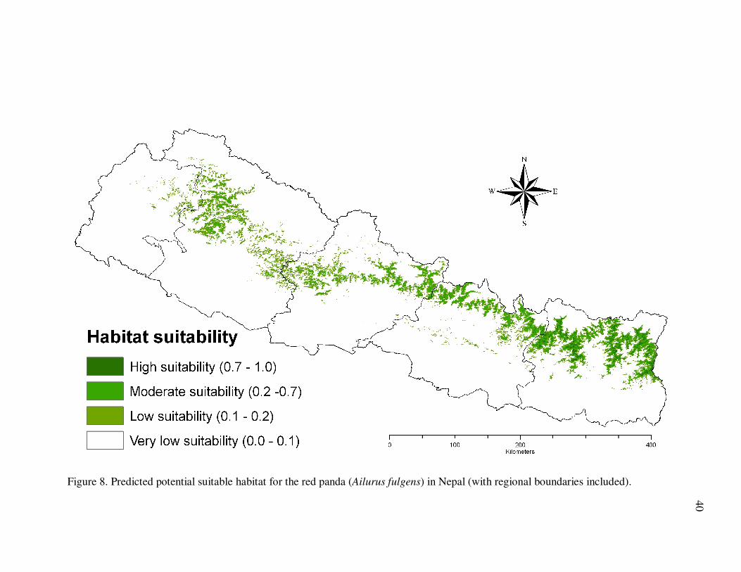
Figure 8. Predicted potential suitable habitat for the red panda (Ailurus fulgens) in Nepal (with regional boundaries included).
40

Figure 9. Predicted potential suitable habitat at 0.5 threshold for red panda (Ailurus fulgens) in Nepal (with regional boundaries
included).
41
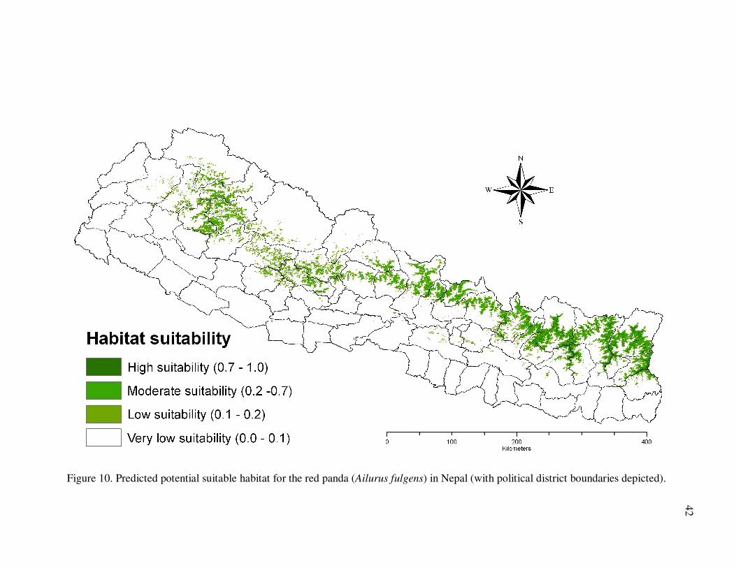
Figure 10. Predicted potential suitable habitat for the red panda (Ailurus fulgens) in Nepal (with political district boundaries depicted).
42

Figure 11. Predicted potential suitable habitat at a 0.5 threshold for the red panda (Ailurus fulgens) in Nepal (with political district
boundaries depicted).
43
44
Relative Importance of Environmental Variables
Elevation was the most important predictor of the red panda distribution (Table 9)
with a total contribution of 37.3% followed by temperature seasonality (20.2%) and tree
cover (12.7%).
Jackknife Test
The jackknife evaluation of relative importance of environmental variables
indicated elevation made the highest contribution to the red panda distribution followed
by temperature seasonality (Fig.13). Elevation had the highest AUC gain when run in
isolation (> 0.91) and the relative loss in AUC was highest when the model was run
without it. AUC gain was the lowest when elevation was removed compared to the
removal of any other single variable. A similar pattern was observed for temperature
seasonality but with a lower magnitude after elevation. Although the AUC loss was small
after removing temperature seasonality, it had the highest gain after elevation when run in
isolation. Precipitation in the coldest quarter followed by precipitation seasonality was
the most important factors after elevation and temperature seasonality. These two
variables had the highest AUC gain (both > 0.72) in isolation after elevation and
temperature seasonality and AUC losses were also significant after removal of these
variables.

45
Table 9. Relative percent contribution of 10 environmental variables (layers) to the red
panda (Ailurus fulgens) distribution in Nepal.
Layers Contribution (%)
Elevation 36.4
Temperature seasonality 21.2
Tree cover 12.8
Winter EVI 6.1
Land cover 5.8
Winter LAI 5.8
Precipitation of coldest quarter 4.3
Precipitation of warmest quarter 3.6
Precipitation seasonality 3.1
Spring NDVI 1.1
46
Figure 12. Receiver operating characteristic curve (Sensitivity vs. 1 – Specificity) on red
panda occurrence training and test data for a predictive model in red panda.
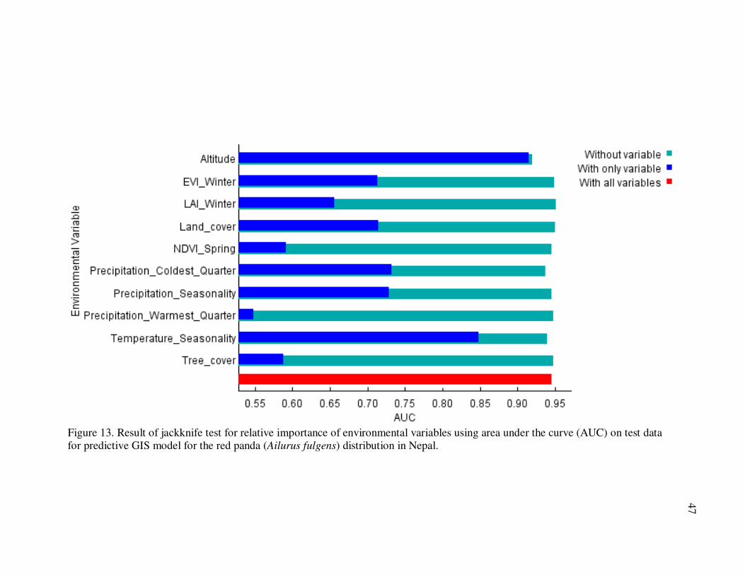
Figure 13. Result of jackknife test for relative importance of environmental variables using area under the curve (AUC) on test data
for predictive GIS model for the red panda (Ailurus fulgens) distribution in Nepal.
47
48
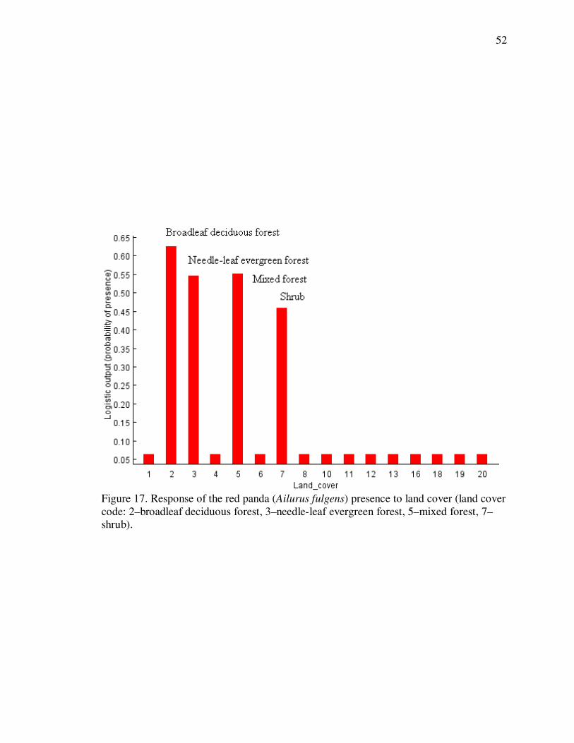
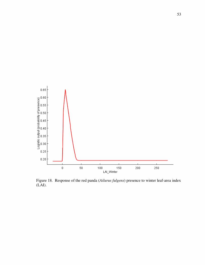
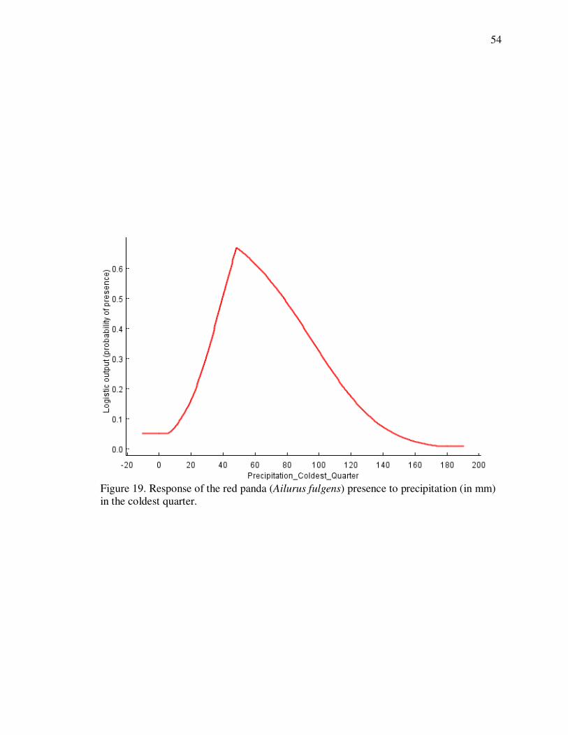
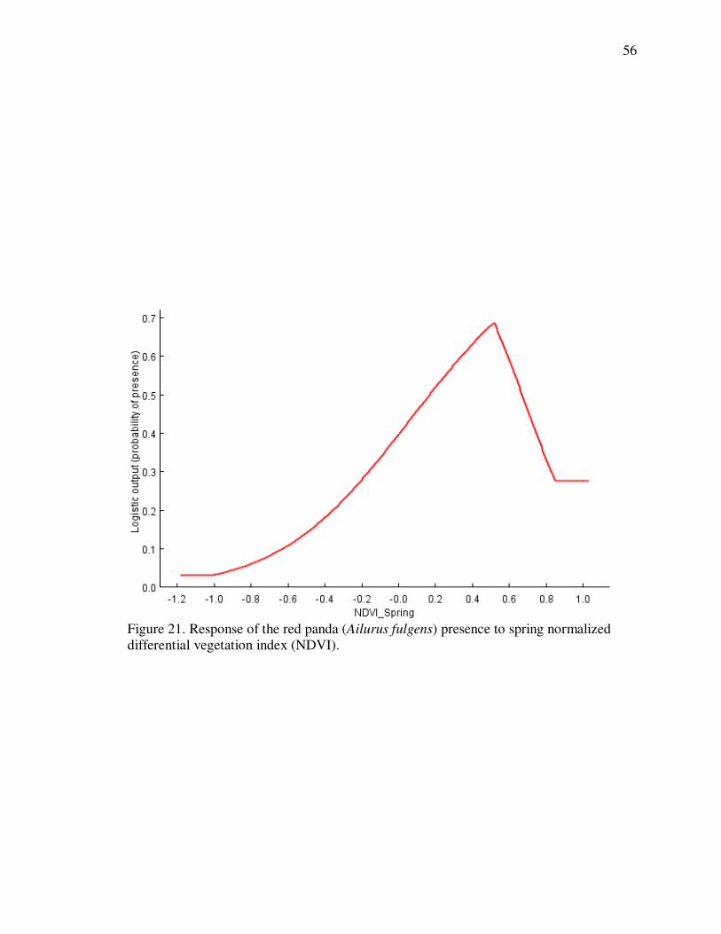
Response of Environmental Factors to Red Panda Distribution
Elevation, the variable with highest relative importance to the MaxEnt model, had
the highest response at a value of 3,000 m (Fig.14). The response of tree cover was
directly proportional to its magnitude, though its response saturated around 75% cover
(Fig.15). The response to the EVI in the winter season was observed between positive
and negative 0.4 with its highest response around an EVI value of 0 (Fig.16). Only four
categories of land cover types since land cover is a categorical variable, showed a
response to the model. Broadleaf deciduous forest had the highest response followed by
needle-leaf evergreen forest and mixed forest, both with a similar magnitude of response,
and shrub with the lowest response (Table 5, Fig.17). The response of winter LAI was
observed between 0 and 40, with the highest response near a value of 10 (Fig.18). The
response of precipitation in the coldest quarter was the highest close to 50 and the
response decreased for higher precipitation and saturated at 160 (Fig.19). The highest
response of precipitation, 1100, was during the warmest quarter (Fig.20). The response of
spring NDVI gradually increased up to a value of 0.5 and then sharply decreased
(Fig.21).

49
Figure 14. Response of the red panda (Ailurus fulgens) presence to elevation (in meters).

50
Figure 15. Response of the red panda (Ailurus fulgens) presence to tree cover.
51
Figure 16. Response of the red panda (Ailurus fulgens) presence to winter enhanced
vegetation index (EVI).
52
Figure 17. Response of the red panda (Ailurus fulgens) presence to land cover (land cover
code: 2–broadleaf deciduous forest, 3–needle-leaf evergreen forest, 5–mixed forest, 7–
shrub).
53
Figure 18. Response of the red panda (Ailurus fulgens) presence to winter leaf-area index
(LAI).
54
Figure 19. Response of the red panda (Ailurus fulgens) presence to precipitation (in mm)
in the coldest quarter.

55
Figure 20. Response of the red panda (Ailurus fulgens) presence to precipitation (in mm)
in warmest quarter.
56
Figure 21. Response of the red panda (Ailurus fulgens) presence to spring normalized
differential vegetation index (NDVI).
57
Conservation Status of Red Panda in Nepal
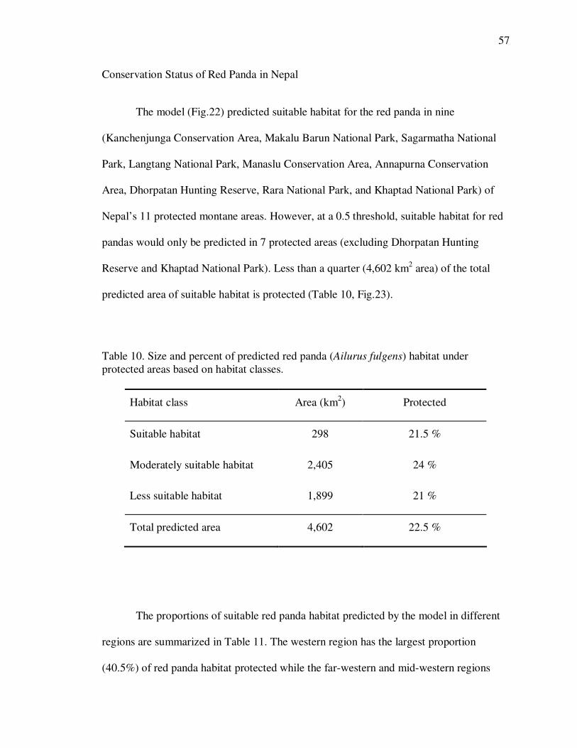
The model (Fig.22) predicted suitable habitat for the red panda in nine
(Kanchenjunga Conservation Area, Makalu Barun National Park, Sagarmatha National
Park, Langtang National Park, Manaslu Conservation Area, Annapurna Conservation
Area, Dhorpatan Hunting Reserve, Rara National Park, and Khaptad National Park) of
Nepal’s 11 protected montane areas. However, at a 0.5 threshold, suitable habitat for red
pandas would only be predicted in 7 protected areas (excluding Dhorpatan Hunting
Reserve and Khaptad National Park). Less than a quarter (4,602 km2 area) of the total
predicted area of suitable habitat is protected (Table 10, Fig.23).
Table 10. Size and percent of predicted red panda (Ailurus fulgens) habitat under
protected areas based on habitat classes.
Habitat class Area (km2) Protected
Suitable habitat 298 21.5 %
Moderately suitable habitat 2,405 24 %
Less suitable habitat 1,899 21 %
Total predicted area 4,602 22.5 %
The proportions of suitable red panda habitat predicted by the model in different
regions are summarized in Table 11. The western region has the largest proportion
(40.5%) of red panda habitat protected while the far-western and mid-western regions

58
had the lowest. However, the western (36.5 %) and eastern (36.2 %) regions had the
largest proportion of protected red panda habitat in the country.
A higher human population growth occurred between 1971 and 2001 in districts
with suitable red panda habitat in all five regions (Table 11). The most extreme growth in
human population density was in the central region which has relatively less red panda
habitat. However, the red panda habitat in the eastern region is under threat due to high
human population growth (67%).
While the eastern region has the largest area (36.4 %) of predicted suitable habitat
for red pandas, only 22.5 % of the suitable red panda habitat in the region is protected
areas. Hence a large proportion of the suitable red panda habitat is still unprotected in this
region. However, a greater proportion of high probability red panda distribution areas fall
within this region, indicating highly suitable red panda habitat exists in this region. This
region also has one of the highest human population growth rates (67% growth since
1971, Table 11) and it continues to grow. The increasing human population in the region,
hence, exerts high anthropogenic pressure on the unprotected, highly suitable red panda
habitats in eastern Nepal.
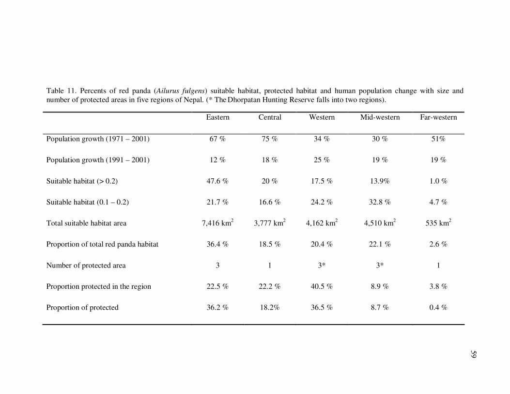
Table 11. Percents of red panda (Ailurus fulgens) suitable habitat, protected habitat and human population change with size and
number of protected areas in five regions of Nepal. (* The Dhorpatan Hunting Reserve falls into two regions).
Eastern Central Western Mid-western Far-western
Population growth (1971 – 2001) 67 % 75 % 34 % 30 % 51%
Population growth (1991 – 2001) 12 % 18 % 25 % 19 % 19 %
Suitable habitat (> 0.2) 47.6 % 20 % 17.5 % 13.9% 1.0 %
Suitable habitat (0.1 – 0.2) 21.7 % 16.6 % 24.2 % 32.8 % 4.7 %
Total suitable habitat area 7,416 km2 3,777 km
2 4,162 km
2 4,510 km
2 535 km
2
Proportion of total red panda habitat 36.4 % 18.5 % 20.4 % 22.1 % 2.6 %
Number of protected area 3 1 3* 3* 1
Proportion protected in the region 22.5 % 22.2 % 40.5 % 8.9 % 3.8 %
Proportion of protected 36.2 % 18.2% 36.5 % 8.7 % 0.4 %
59

Figure 22. Predicted potential suitable habitat for the red panda (Ailurus fulgens) within protected areas in Nepal.
60

Figure 23. Predicted potential suitable habitat at 0.5 threshold within protected areas for the red panda (Ailurus fulgens) in Nepal.
61

62
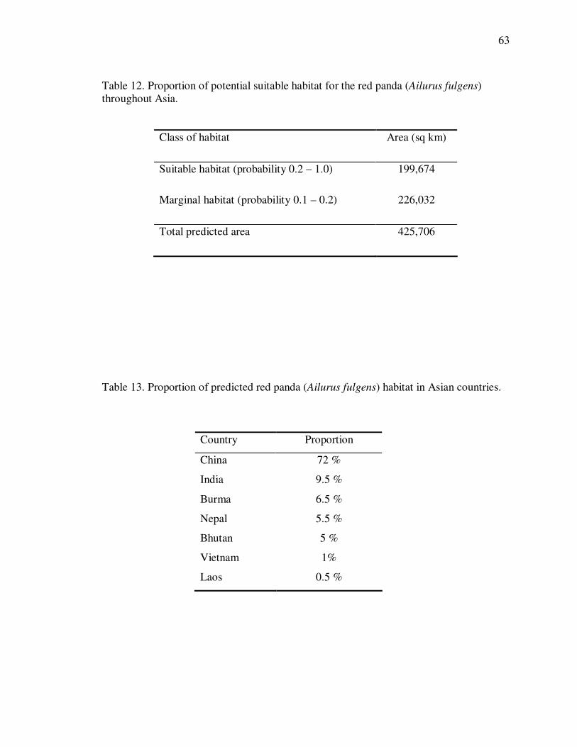
Red Panda Habitat Projection at Global Scale
I also projected the distribution model to an area larger than Nepal to predict the
red panda distribution throughout Asia. A total area of 425,700 km2 (Table 12) was
predicted as suitable red panda habitat in seven countries: Nepal, India, Bhutan, China,
Myanmar (Burma), Laos and Vietnam (Fig.24). The projected model predicted a global
distribution of the red panda as far west as western Nepal and as far east as northwestern
Vietnam. Based on a commonly used threshold of 0.5, predicted suitable habitat occurs in
approximately 34,380 km2 mostly in Nepal and China with smaller areas in Bhutan,
India, Myanmar and Vietnam (Fig.25).
I projected the prediction of the red panda potential distribution to other countries
based on the red panda occurrence in Nepal. This may lead to inaccurate and bias
predictions in the other countries. Therefore, I used two classes to roughly estimate the
extent of the red panda distribution in these countries (Table 12). I also estimated the
proportion of red panda habitat in the different countries. China had the largest proportion
of red panda habitat (72%) followed by India (9.5%). Nepal had only 5.5% of the total
suitable area for the red panda. Laos had a smallest proportion of predicted red panda
habitat (0.5%, Table 13).
63
Table 12. Proportion of potential suitable habitat for the red panda (Ailurus fulgens)
throughout Asia.
Class of habitat Area (sq km)
Suitable habitat (probability 0.2 – 1.0) 199,674
Marginal habitat (probability 0.1 – 0.2) 226,032
Total predicted area 425,706
Table 13. Proportion of predicted red panda (Ailurus fulgens) habitat in Asian countries.
Country Proportion
China 72 %
India 9.5 %
Burma 6.5 %
Nepal 5.5 %
Bhutan 5 %
Vietnam 1%
Laos 0.5 %

Figure 24. Predicted potential suitable habitat for the red panda (Ailurus fulgens) in Asia.
64

Figure 25. Predicted potential suitable habitat at 0.5 threshold for the red panda (Ailurus fulgens) in Asia.
65

66
DISCUSSION
The MaxEnt species distribution modeling basically maps the fundamental niche
of a species which is different from an occupied niche and usually larger than the
fundamental niche (Pearson 2007). Such models usually over-predict the species
distribution because the area predicted as suitable habitat is the fundamental niche of a
species even though the species may not occur in that area due to other factors, e.g.,
anthropogenic factors. Though these models have higher sensitivity, they may have less
specificity.
The MaxEnt model of the red panda distribution in Nepal predicted suitable red
panda habitat at a higher success rate with as low an omission rate as 11.6 %. The
predicted red panda distribution approximates the anecdotally known and even the
systematically confirmed distribution of the red panda in Nepal (Glatston 1994, Yonzon
et al. 1997). The model predicted the western limit of the red panda distribution in the
far-west region of Nepal in Bajura and Bajhang districts located close to the western
known limit of the red panda distribution in Mugu District (Glatston 1994). Just east of
these districts, the red panda has been reported from Jumla District (Yonzon et al. 1997)
and from Rara National Park in Mugu District (Sharma 2009). Therefore, at this extent, it
is equally likely that the red panda distribution may have been over-predicted or the red
panda is simply yet unreported from the area west of Mugu District. However, the
omission rate of 11.6 % and the careful observation of predicted logistic value for all 106

67
red panda occurrence points (Fig.7) also indicates slight under-prediction of red panda
suitable habitat in Nepal.
The red panda distribution has also been over-predicted in the central lower
mountains in small patches. These areas may be suitable as the fundamental niche of the
red panda; however, these small and fragmented patches are probably unsuitable due to a
lack of connectivity. Alternately, these areas have very dense human populations, and
hence at a finer scale may be unsuitable for red pandas. While resolution of analysis has
little influence on the model (Guisan et al. 2007), the resolution of this study (1 km) at
the national scale cannot capture settlements and defragmentation in forest cover within a
pixel, and hence the model may over-predict the suitable areas. However, overlaying of a
finer resolution forest cover for smaller scale analysis will reduce the total suitable area.
A GIS-based overlay analysis at a resolution of 0.25 km2 (Yonzon et al. 1997), estimated
only 912 km2
of area suitable for the red panda in Nepal. This analysis used only three
parameters – area with fir forest within an elevational range of 3,000 – 4,000 m with
annual precipitation > 2,000 mm. However, the red panda has been recorded beyond this
elevation range, e.g., at 2,800 m in the Kanchenjunga region (Mahato 2004a) and as low
as 2,400 m in Ilam and Panchthar districts (pers. obs. 2007) and in Sinhalila National
Park in India (Pradhan et al. 2001). Likewise, the red panda has been recorded in other
forest types, e.g., pine forest in the Everest region (Mahato 2004b), Rhododendron forest
and mixed broadleaf forest in eastern Nepal (pers. obs. 2006, 2007) and in Singhalila
National Park (Pradhan et al. 2001). Therefore, Yonzon et al. (1997) may have
underestimated the red panda distribution.

68
Despite a reasonable probability of over-prediction and slight under-prediction in
suitable red panda area and a coarse grain size, this model provides a baseline for further
investigation. It provides an understanding of the red panda distribution at a landscape
level on a national scale. Furthermore, projection of the model to other countries provides
a better understanding of the global red panda distribution. The model is helpful in
conservation planning (Rodriguez et al. 2007) and in the identification and prioritization
of sites for further ground-truth investigation. With the help of this model, a fine-scale
distribution map can also be prepared to determine the red panda distribution more
precisely. The fact that most of the known locations of the red panda were confirmed in
the recent decade (Mahato 2004a, Mahato 2004b, Regmi 2009, Sharma and Kandel 2007,
Sharma 2009, Subedi 2009) is evidence that ground-truth information on the red panda
distribution is not well understood in Nepal. Therefore, this model can be used as a tool
in identifying potential areas and planning for ground-truthing surveys of the red panda
distribution at a reduced cost in both time and money. This is particularly important for
rare and elusive species like the red panda.
The predictor variables used to build this model were selected based on the
available ecological information on the red panda. The selection of variables was also
based on the resolution of analysis. For instance, there are other variables which are
important predictors of the red panda distribution, e.g., aspect, slope. However, I could
not incorporate these variables at the coarse resolution necessitated by the available
habitat and ecological layers. However, these and several additional variables, e.g.,
distance to water, distance from settlement etc., may be important variables to consider in
the future construction of a finer resolution distribution map.

69
REFERENCES
Austin, M. 2002. Spatial prediction of species distribution: an interface between
ecological theory and statistical modeling. Ecological Modeling. 157:101-118.
Brotons, L., W. Thuiller, M. B. Araújo, and A. H. Hirzel. 2004. Presence-absence versus
presence-only modeling methods for predicting bird habitat suitability.
Ecography. 27:437-448.
Carlson, T. N. and D. R. Ripley. 1997. On the relation between NDVI, fractional
vegetation cover, and leaf-area index. Remote Sensing of Environment. 62:241-
252.
Choudhary, A. 2001. An overview of the status and conservation of the red panda Ailurus
fulgens in India, with reference to its global status. Oryx. 35:250-259.
Cohen, J. 1960. A coefficient of agreement for nominal scales. Educational and
Psychological Measurement. 20:37-46.
Corsi, F., E. Dupre, and L. Boitani. 1999. A large-scale model of wolf distribution in
Italy for conservation planning. Conservation Biology. 13:150-159.
Curran, P. J. and M. D. Steven. 1983. Multispectral Remote Sensing for the Estimation of
Green Leaf Area Index [and Discussion]. Philosophical Transactions of the Royal
Society of London. Series A, Mathematical and Physical Sciences. 309(1508):
257-270.
Decker, D. M. and W. C. Wozencraft. 1991. Phylogenetic analysis of recent procyonid
genera. Journal of Mammology. 72: 42-55.
Doko, T. 2007. Modeling of species geographic distribution for assessing present needs
for the ecological networks – case study of Fuji region and Tanzawa region,
Japan. M.Sc. thesis submitted to ITC, Enschede, The Netherlands.
Eisenberg, J. F. 1981. The Mammalian radiations: an analysis of trends in evolution,
adaptation and behavior. University of Chicago Press. Chicago.
70
Fielding, A. H. and J. F. Bell. 1997. A review of methods for the assessment of prediction
errors in conservation presence/absence models. Environmental Conservation.
24(1):38-49
Glatston, A. R. 1994. The Red panda, Olingos, Coatis, Raccoons and their relatives.
Status Survey and Conservation Action Plan for Procoyonids and Ailurids.
IUCN/SSC Mustelid, Viverrid, and Procyonid Specialist Group. IUCN, Gland,
Switzerland.
Graham, M. H. 2003. Confronting multicollinearity in ecological multiple regression.
Ecology. 84(11):2809-2815.
Guisan, A. and W. Thuiller. 2005. Predicting species distribution: Offering more than
simple habitat models. Ecological Letters. 8:993-1009
Guisan, A., T. C. Edwards, Jr., and T. Hastie. 2002. Generalized linear and generalized
additive models in studies of species distributions: setting the scene. Ecological
Modeling. 157:89-100.
Guisan, A., O. Broennimann, M. Engler, M. Vust, N. G. Yoccoz, A. Lehman, and N.E.
Zimmermann. 2006. Using niche-based models to improve the sampling of rare
species. Conservation Biology. 20:501-511.
Guisan A, C. H. Graham, J. Elith, F. Huettmann, and the NCEAS Species Distribution
Modelling Group. 2007. Sensitivity of predictive species distribution models to
change in grain size. Diversity and Distribution. 13:332-340.
Hijmans, R. J., S. E. Cameron, J. L. Parra, P. G. Jones, and A. Jarvis. 2005. Very high
resolution interpolated climate surfaces for global land areas. International
Journal of Climatology. 25:1965-1978.
Hirzel, A. H., J. Hausser, D. Chessel, and N. Perrin. 2002. Ecological-niche factor
analysis: How to compute habitat-suitability map without absence data. Ecology.
83:2027-2036.
HMGN/MFSC. 2002. Nepal Biodiversity Strategy, Ministry of Forests and Soil
Conservation, His Majesty’s Government of Nepal. pp 170.
Huete, A., K. Didan, T. Miura, E. P. Rodriguez, X. Gao, and L. G. Ferreira. 2002.
Overview of the radiometric and biophysical performance of the MODIS
vegetation indices. Remote Sensing of Enviroment. 83:195-213.
71
IUCN. 2010. IUCN Red list of threatened species. Version 2010.1. <www.redlist.org>.
Downloaded on 23 June 2010.
Lai, J. 2009. Amphibian species distribution modeling in Poland. M.Sc. thesis. ITC,
Enchede, the Netherland. pp 78.
Jimenez-Valverde, A. and J. M. Lobo. 2007. Threshold criteria for conversion of
probability of species presence to either-or presence-absence. Acta Oecologica-
International Journal of Ecology. 31:361-369.
Johnson, K. G., G. B. Schaller, and H. Jinchu. 1988. Comparative behavior of red and
giant panda in the Wolong Reserve, China. Journal of Mammology. 69:552-564.
Kumar, S. and T. J. Stohlgren. 2009. Maxent modeling for predicting suitable habitat for
threatened and endangered tree Canacomyrica monticola in New
Caledonia. Journal of Ecology and Natural Environment. 1(4):94-98.
Kumar, S., S. A. Spaulding, T. J. Stohlgren, K. A. Hermann, T. S. Schmidt, and L. L.
Bahls. 2009. Predicting habitat distribution for the freshwater diatom
Didymosphenia geminata in the continental US. Frontiers in Ecology and the
Environment. 7(8):415-420.
Leathwick, J. R., D. Rowe, J. Richardson, J. Elith, and T. Hastie. 2005. Using
multivariate adaptive regression splines to predict the distribution of New
Zealand's freshwater diadromous fish. Freshwater Biology. 50:2034-2052.
Leone, C. A. and A. L. Wiens. 1956. Comparative serology of carnivores. Journal of
Mammology. 37:11-23.
Liu, C., P. M. Berry, T. P. Dawson, and R. G. Pearson. 2005. Selecting thresholds of
occurrence in the prediction of species distributions. Ecography. 28:385-393.
LP DAAC. 2008. MODIS Overview. Retrieved from:
https://lpdaac.usgs.gov/lpdaac/products/modis_overview. National Aeronautics
and Space Administration, U.S. Geological Survey. Accessed on March 13, 2010.
Mahato, N. K. 2004a. Status of Red panda Ailurus fulgens in Kangchenjunga region.
Tigerpaper. 31(4):7-9.
Mahato, N. K. 2004b. Baseline survey of Red panda Ailurus fulgens status in the
buffer zone of Sagarmatha National Park. A report submitted to WWF Nepal
Program, Kathmandu, Nepal.

72
Manel, S., J. M. Dias, and S. J. Ormerod. 1999. Comparing discriminant analysis, neural
networks and logistic regression for prediction species distributions: a case study
with a Himalayan river bird. Ecological Modelling. 120:337-347.
Manel, S., H. C. Williams, and S. J. Ormerod. 2001. Evaluating presence-absence models
in ecology: the need to account for prevalence. Journal of Applied Ecology. 38(5):
921-931.
Matsushita, B., W. Yang, J. Chen, Y. Onda, and G. Qiu. 2007. Sensitivity of the
enhanced vegetation index (EVI) and normalized difference vegetation index
(NDVI) to topographic effects: A case study in high-density cypress forest.
Sensors. 7:2636-2651.
Negga, H. E. 2007. Predictive modeling of amphibian distribution using ecological
survey data: a case study of Central Portugal. M.Sc. thesis. ITC, Enchede, the
Netherland. pp 74.
O’Brien, S. J., W. G. Nash. D. E. Wildt. M. E. Bush, and R. E. Benveniste. 1985. A
molecular solution to the riddle of the giant panda’s physiology. Nature. 317:140-
144.
Olsen, D. M. and E. Dinerstein. 1998. The Global 200: A Representation Approach to
Conserving the Earth’s Most Biologically Valuable Eco-regions. Conservation
Biology. 12:502-515.
Pearce, J. and S. Ferrier. 2000. Evaluating the predictive performance of habitat models
developed using logistic regression. Ecological Modeling. 133:225-245.
Pearce, J. and D. B. Lindenmayer. 1998. Bioclimatic analysis to enhance reintroduction
biology of the endangered helmeted honeyeater (Lichenostomus melanops
cassidix) in southeastern Australia. Restoration Ecology. 6:238-243.
Pearson, R. G. 2007. Species’ distribution modeling for conservation educators and
practitioners. Synthesis. American Museum of Natural History. Available at
http://ncep.amnh.org.
Pearson, R. G., T. P. Dawson, and C. Liu. 2004. Modelling species distributions in
Britain: A hierarchical integration of climate and land-cover data. Ecography.
27:285-298.
Pearson, R.G., C. J. Raxworthy, M.Nakamura, and T. Peterson. 2007. Predicting species
distributions from small numbers of occurrence records: a test case using cryptic
geckos in Madagascar. Journal of Biogeography. 34:102–117.
73
Pearson, R. G., W. Thuiller, M. B. Araújo, E. Martinez-Meyer, L. Brotons, C. McClean,
L. Miles, P. Segurado, T. P. Dawson, and D. Lees. 2006. Model-based uncertainty
in species' range prediction. Journal of Biogeography. 33:1704-1711.
Pettorelli, N., J. O. Vik, A. Mysterud, J. Gaillard, C. J. Tucker, and N. C. Stenseth. 2005.
Using the satellite-derived NDVI to assess ecological responses to environmental
change. Trends in Ecology and Evolution. 20(9):503-510.
Phillips, S. J., R. P. Anderson, and R. E. Schapire. 2006. Maximum entropy modeling of
species geographic distributions. Ecological Modeling. 190:231-259.
Pradhan, S., G. K. Shah, and J. A. Khan. 2001. Ecology of the red panda, Ailurus fulgens
in the Singhalila National Park, Darjeeling, India. Biological Conservation.
98:11-18.
Reed, B. C., J. F. Brown, D. VanderZee, T. R. Loveland, J. W. Merchant, and D. O.
Ohlen. 1994. Measuring Phenological Variability from Satellite Imagery. Journal
of Vegetation Science. 5(5):703-714.
Regmi, G. R. 2009. The Red panda (Ailurus fulgens) in Langtang National Park: an
assessment of its conservation status. NEF Newsletter. 18:69-70.
Reid, D. G., H. Jinchu, and Y. Huang. 1991. Ecology of the red panda Ailurus fulgens in
the Wolong Reserve, China. Journal of Zoology. 225:347-364.
Roberts, M. and J. Gittleman. 1984. Ailurus fulgens. Mammalian Species. 222:1-8.
Roberts, M. S. 1981. The Reproductive Biology of the Red Panda. Unpublished MS
thesis. University of Maryland, College Park.
Robertson, M. P., N. Caithness, and M. H. Villet. 2001. A PCA-based modeling
technique for predicting environmental suitability for organisms from presence
records. Diversity and Distributions. 7:15-27.
Rodriguez, J. P., L. Brotons, J. Bustamante, and J. Seoane. 2007. The application of
predictive modeling of species distribution to biodiversity conservation. Diversity
and Distributions. 13:243-251.
RPN. 2006-2009. Internal progress report. Red Panda Network-Nepal, Kathmandu,
Nepal.
74
Sharma, H. 2009. Distribution and conservation status of red panda (Ailurus fulgens) in
the Rara National Park, Nepal. A paper presented at 23rd
Annual meeting and
2009 International Congress for Conservation Biology, China.
Sharma, H. P. and R. N. Kandel. 2007. Red panda (Ailurus fulgens) in the Dhorpatan
Hunting Reserve of Nepal: an assessment of their conservation status. A report to
People’s Trust for Endangered Species, UK.
Steffens, E. 2004. Red pandas and conservation: Political ecology, tenure, livestock and
hunting in high altitude forests of Nepal. M.Sc. thesis submitted to University of
Wisconsin-Madison.
Stockwell, D. and D. Peters. 1999. The GARP modelling system: problems and solutions
to automated spatial prediction. International Journal of Geographical
Information Science. 13:143-158.
Story, M. and R. G. Congalton. 1986. Accuracy assessment: a user’s perspective.
Photogrammetric Engineering and Remote Sensing. 52(3):397-399.
Subedi, T. R. 2009. Habitat, Status and Conservation of Red Panda (Ailurus fulgens) in
Dhorpatan Hunting Reserve, Nepal. A report to Rufford Small Grants, UK.
Thuiller, W., D. M. Richardson, P. Pysek, G. F. Midgley, G. O. Hughes, and M. Rouget.
2005. Niche-based modeling as a tool for predicting the global risk of alien plant
invasions. Global Change Biology. 11:2234-2250.
Udvardy, M. D. F. 1975. A classification of the biogeographical provinces of the world.
IUCN occasional paper No. 18, IUCN, Switzerland.
Warnell, K. J. 1988. Feed intake, digestibility, digesta passage, and fecal microbial
ecology of the red panda (Ailurus fulgens). Unpublished M.Sc. thesis submitted to
Michigan State University. East Lansing, MI.
Wayne, R. K., R. E. Benveniste, E. Janczewski, and S. J. O’Brien. 1989. Molecular and
Biochemical evolution of the Carnivora. pp. 465-494 in Carnivore Behavior,
Ecology and Evolution (Gittleman, J. L. ed.), Chapman and Hall, London.
Wei, F., Z. Feng, Z. Wang, and Z. Hu. 1999. Current distribution, status and conservation
of wild red pandas Ailurus fulgens in China. Biological Conservation. 89:285-
291.
Wurster, D. H. and K. Benirschke. 1968. Comparative cytogenetic studies in the Order
Carnivora. Chromosoma. 24:336-382.
75
Yonzon, P. 1989. Ecology and conservation of red panda in the Nepal-Himalayas. Ph.D.
thesis submitted to University of Maine, Orone.
Yonzon, P. B. and M. L. Hunter. 1991. Conservation of the Red Panda Ailurus fulgens.
Biological Conservation. 57:1-11.
Yonzon, P., P. Yonzon, C. Chaudhary, and B. Vaidya. 1997. Status of the red panda in
the Himalaya. Resources Nepal, Kathmandu. pp 21.
VITA
Naveen K. Mahato obtained a B.Sc. in Forestry from Institute of Forestry at Tribhuvan
University, Nepal in 2003, with an emphasis in Wildlife. As a freelancer, he led a few
wildlife surveys in the Himalaya of Nepal. He worked with WWF Nepal for a year and
was seconded to Nepal’s Department of National Parks and Wildlife Conservation to
assist in CITES implementation. He initiated a non-profit “Red Panda Network”
dedicated to conservation of Red panda in 2006 and led the team until 2007. In January
2008, he entered Texas State University-San Marcos as a Master student in Wildlife
Ecology with an interest in learning principles in wildlife conservation. At Texas State,
he has worked as an Instructional Assistant at Department of Biology. He has a keen
interest in Himalayan wildlife, especially in the mammals.
Permanent Address: Simara – 5, Sarlahi, NEPAL
Email: [email protected]
This thesis was typed by Naveen K. Mahato.