Distribution of Mutual Information

Marcus Hutter IDSIA, Galleria 2, CH-6928 Manno-Lugano, Switzerland

marcus@idsia.ch http://www.idsia.ch/- marcus

Abstract

The mutual information of two random variables z and J with joint probabilities {7rij} is commonly used in learning Bayesian nets as well as in many other fields. The chances 7rij are usually estimated by the empirical sampling frequency nij In leading to a point es­timate J(nij In) for the mutual information. To answer questions like "is J (nij In) consistent with zero?" or "what is the probability that the true mutual information is much larger than the point es­timate?" one has to go beyond the point estimate. In the Bayesian framework one can answer these questions by utilizing a (second order) prior distribution p( 7r) comprising prior information about 7r. From the prior p(7r) one can compute the posterior p(7rln), from which the distribution p(Iln) of the mutual information can be cal­culated. We derive reliable and quickly computable approximations for p(Iln). We concentrate on the mean, variance, skewness, and kurtosis , and non-informative priors. For the mean we also give an exact expression. Numerical issues and the range of validity are discussed.

1 Introduction

The mutual information J (also called cross entropy) is a widely used information theoretic measure for the stochastic dependency of random variables [CT91, SooOO] . It is used, for instance, in learning Bayesian nets [Bun96, Hec98] , where stochasti­cally dependent nodes shall be connected. The mutual information defined in (1) can be computed if the joint probabilities {7rij} of the two random variables z and J are known. The standard procedure in the common case of unknown chances 7rij is to use the sample frequency estimates n~; instead, as if they were precisely known probabilities; but this is not always appropriate. Furthermore, the point estimate J (n~; ) gives no clue about the reliability of the value if the sample size n is finite. For instance, for independent z and J, J(7r) =0 but J(n~;) = O(n- 1 / 2 ) due to noise in the data. The criterion for judging dependency is how many standard deviations J(":,;) is away from zero. In [KJ96, Kle99] the probability that the true J(7r) is greater than a given threshold has been used to construct Bayesian nets. In the Bayesian framework one can answer these questions by utilizing a (second order)

prior distribution p(7r),which takes account of any impreciseness about 7r . From the prior p(7r) one can compute the posterior p(7rln), from which the distribution p(Iln) of the mutual information can be obtained.

The objective of this work is to derive reliable and quickly computable analytical expressions for p(1ln). Section 2 introduces the mutual information distribution, Section 3 discusses some results in advance before delving into the derivation. Since the central limit theorem ensures that p(1ln) converges to a Gaussian distribution a good starting point is to compute the mean and variance of p(1ln). In section 4 we relate the mean and variance to the covariance structure of p(7rln). Most non-informative priors lead to a Dirichlet posterior. An exact expression for the mean (Section 6) and approximate expressions for the variance (Sections 5) are given for the Dirichlet distribution. More accurate estimates of the variance and higher central moments are derived in Section 7, which lead to good approximations of p(1ln) even for small sample sizes. We show that the expressions obtained in [KJ96, Kle99] by heuristic numerical methods are incorrect. Numerical issues and the range of validity are briefly discussed in section 8.

2 Mutual Information Distribution

We consider discrete random variables Z E {l, ... ,r} and J E {l, ... ,s} and an i.i.d. random process with samples (i,j) E {l , ... ,r} x {l, ... ,s} drawn with joint probability 7rij. An important measure of the stochastic dependence of z and J is the mutual information

T S 7rij

1( 7r) = L L 7rij log ~ = L 7rij log 7rij - L 7ri+ log7ri+ - L 7r +j log7r +j' (1) i=1 j = 1 H +J ij i j

log denotes the natural logarithm and 7ri+ = Lj7rij and 7r +j = L i7rij are marginal probabilities. Often one does not know the probabilities 7rij exactly, but one has a sample set with nij outcomes of pair (i,j). The frequency irij := n~j may be used as a first estimate of the unknown probabilities. n:= L ijnij is the total sample size. This leads to a point (frequency) estimate 1(ir) = Lij n~j logn:~:j for the mutual informat ion (per sample).

Unfortunately the point estimation 1(ir) gives no information about its accuracy. In the Bayesian approach to this problem one assumes a prior (second order) prob­ability density p( 7r) for the unknown probabilities 7rij on the probability simplex. From this one can compute the posterior distribution p( 7rln) cxp( 7r) rrij7r~;j (the nij are multinomially distributed). This allows to compute the posterior probability density of the mutual information.1

p(Iln) = f 8(1(7r) - I)p(7rln)dTS 7r (2)

2The 80 distribution restricts the integral to 7r for which 1(7r) =1. For large sam-

1 I(7r) denotes the mutual information for the specific chances 7r, whereas I in the context above is just some non-negative real number. I will also denote the mutual information random variable in the expectation E [I] and variance Var[I]. Expectaions are always w.r.t. to the posterior distribution p(7rln).

2Since O~I(7r) ~Imax with sharp upper bound Imax :=min{logr,logs}, the integral may

be restricted to J:mam, which shows that the domain of p(Iln) is [O,Imax] .

pIe size n ---+ 00, p(7rln) is strongly peaked around 7r = it and p(Iln) gets strongly peaked around the frequency estimate I = I(it). The mean E[I] = fooo Ip(Iln) dI = f I(7r)p(7rln)dTs 7r and the variance Var[I] =E[(I - E[I])2] = E[I2]- E[Ij2 are of cen­tral interest.

3 Results for I under the Dirichlet P (oste )rior

Most3 non-informative priors for p(7r) lead to a Dirichlet posterior distribution ( I) IT nij -1 ·th· t t t· -,,, h ' th b p 7r n ex: ij 7rij WI III erpre a IOn nij - nij + nij , were nij are e num er

of samples (i,j), and n~j comprises prior information (1 for the uniform prior, ~ for Jeffreys' prior, 0 for Haldane's prior, -?:s for Perks' prior [GCSR95]). In principle this allows to compute the posterior density p(Iln) of the mutual information. In sections 4 and 5 we expand the mean and variance in terms of n-1 :

E[I] ~ nij I nijn (r - 1)(8 - 1) O( -2) L...J - og --- + + n , .. n ni+n+j 2n 'J

(3)

Var[I]

The first term for the mean is just the point estimate I(it). The second term is a small correction if n » r· 8. Kleiter [KJ96, Kle99] determined the correction by Monte Carlo studies as min {T2~1 , 8;;;,1 }. This is wrong unless 8 or rare 2. The expression 2E[I]/n they determined for the variance has a completely different structure than ours. Note that the mean is lower bounded by co~st. +O(n- 2 ), which is strictly positive for large, but finite sample sizes, even if z and J are statistically independent and independence is perfectly represented in the data (I (it) = 0). On the other hand, in this case, the standard deviation u= y'Var(I) '" ~ ",E[I] correctly indicates that the mean is still consistent with zero.

Our approximations (3) for the mean and variance are good if T~8 is small. The central limit theorem ensures that p(Iln) converges to a Gaussian distribution with mean E[I] and variance Var[I]. Since I is non-negative it is more appropriate to approximate p(II7r) as a Gamma (= scaled X2 ) or log-normal distribution with mean E[I] and variance Var[I], which is of course also asymptotically correct.

A systematic expansion in n -1 of the mean, variance, and higher moments is possible but gets arbitrarily cumbersome. The O(n- 2) terms for the variance and leading order terms for the skewness and kurtosis are given in Section 7. For the mean it is possible to give an exact expression

1 E[I] = - L nij[1jJ(nij + 1) -1jJ(ni+ + 1) -1jJ(n+j + 1) + 1jJ(n + 1)] (4)

n .. 'J

with 1jJ(n+1)=-,),+L~=lt=logn+O(~) for integer n. See Section 6 for details and more general expressions for 1jJ for non-integer arguments.

There may be other prior information available which cannot be comprised in a Dirichlet distribution. In this general case, the mean and variance of I can still be

3But not all priors which one can argue to be non-informative lead to Dirichlet poste­riors. Brand [Bragg] (and others), for instance, advocate the entropic prior p( 7r) ex e-H(rr).

related to the covariance structure of p(7fln), which will be done in the following Section.

4 Approximation of Expectation and Variance of I

In the following let frij := E[7fij]. Since p( 7fln) is strongly peaked around 7f = fr for large n we may expand J(7f) around fr in the integrals for the mean and the variance. With I:::.. ij :=7fij -frij and using L: ij7fij = 1 = L:ijfrij we get for the expansion of (1)

( fr .. ) 1:::..2 . 1:::..2 1:::.. 2 . J(7f) = J(fr) + 2)og ~ I:::.. ij + L ----}J-- L ~-L ~+O(1:::..3). (5)

.. 7fi+7f+j .. 27fij . 27fi+ . 27f+j 2J 2J 2 J

Taking the expectation, the linear term E[ I:::.. ij ] = a drops out. The quadratic terms E[ I:::.. ij I:::..kd = Cov( 7fij ,7fkl) are the covariance of 7f under distribution p( 7fln) and are proportional to n-1 . It can be shown that E[1:::..3] ,,-,n-2 (see Section 7).

[ ] ( A) 1", (bikbjl bik bjl) ( ) (-2) EJ = J7f +-~ -A- - -A- - -A- COV7fij,7fkl +On . 2 ijkl 7fij 7fi+ 7f +j

(6)

The Kronecker delta bij is 1 for i = j and a otherwise. The variance of J in leading order in n - 1 is

(7)

where :t means = up to terms of order n -2. So the leading order variance and the leading and next to leading order mean of the mutual information J(7f) can be expressed in terms of the covariance of 7f under the posterior distribution p(7fln).

5 The Second Order Dirichlet Distribution

Noninformative priors for p(7f) are commonly used if no additional prior information is available. Many non-informative choices (uniform, Jeffreys' , Haldane's, Perks',

prior) lead to a Dirichlet posterior distribution:

1 II n;j - 1 ( ) N(n) .. 7fij b 7f++ - 1 with normalization 2J

N(n) (8)

where r is the Gamma function, and nij = n~j + n~j, where n~j are the number of samples (i,j), and n~j comprises prior information (1 for the uniform prior, ~ for Jeffreys' prior, a for Haldane's prior, -!s for Perks' prior) . Mean and covariance of p(7fln) are

A E[] nij 7fij:= 7fij =-, n

(9)

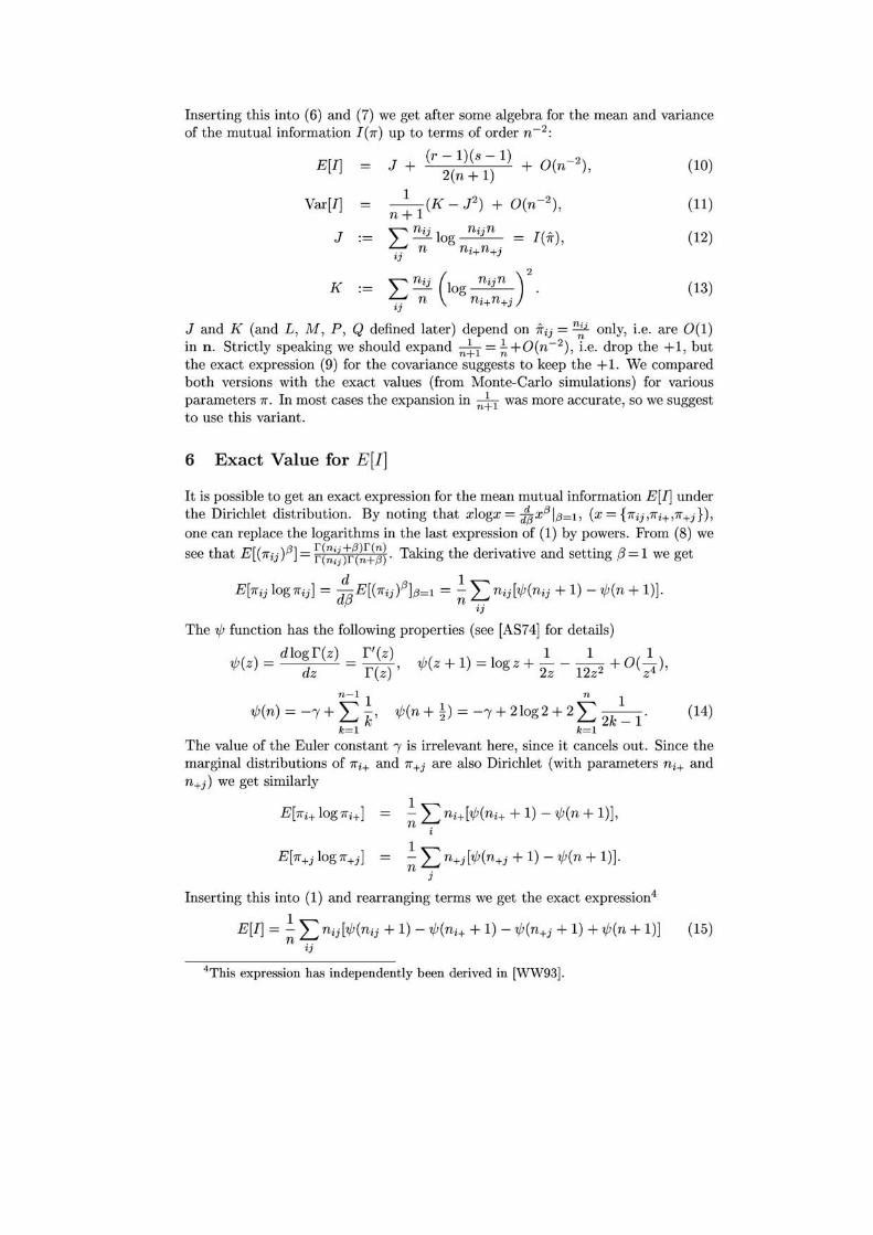
Inserting this into (6) and (7) we get after some algebra for the mean and variance of the mutual information I(7r) up to terms of order n- 2 :

E[I] J (r - 1)(8 - 1) O( -2) + 2(n + 1) + n , (10)

Var[I] ~1 (K - J2) + 0(n-2), n+

(11)

(12)

(13)

J and K (and L, M, P, Q defined later) depend on 7rij = ":,j only, i.e. are 0(1) in n. Strictly speaking we should expand n~l = ~+0(n-2), i.e. drop the +1, but the exact expression (9) for the covariance suggests to keep the +1. We compared both versions with the exact values (from Monte-Carlo simulations) for various parameters 7r. In most cases the expansion in n~l was more accurate, so we suggest to use this variant.

6 Exact Value for E[I]

It is possible to get an exact expression for the mean mutual information E[I] under the Dirichlet distribution. By noting that xlogx= d~x,6I,6= l' (x = {7rij,7ri+ ,7r+j}),

one can replace the logarithms in the last expression of (1) by powers. From (8) we

see that E[ (7rij ),6] = ~i~:~ t~~~;l. Taking the derivative and setting ,8 = 1 we get

d 1 E[7rij log 7rij] = d,8E[(7rij) ,6 ],6=l = ;;: 2:::: nij[1j!(nij + 1) -1j!(n + 1)].

"J

The 1j! function has the following properties (see [AS74] for details)

dlogf(z) f'(z) 1 1 1 1j!(z) = dz = f(z)' 1j!(z + 1) = log z + 2z - 12z2 + O( Z4)'

n - l 1 n 1 1j!(n) = -"( + L k' 1j!(n +~) = -"( + 2log2 + 2 L 2k _ l' (14)

k=l k=l

The value of the Euler constant "( is irrelevant here, since it cancels out. Since the marginal distributions of 7ri+ and 7r+j are also Dirichlet (with parameters ni+ and n+j) we get similarly

1 - L n+j[1j!(n+j + 1) -1j!(n + 1)]. n .

J

Inserting this into (1) and rearranging terms we get the exact expression4

1 E[I] = - L nij[1j! (nij + 1) -1j!(ni+ + 1) -1j!(n+j + 1) + 1j!(n + 1)] (15)

n ..

4This expression has independently been derived in [WW93].

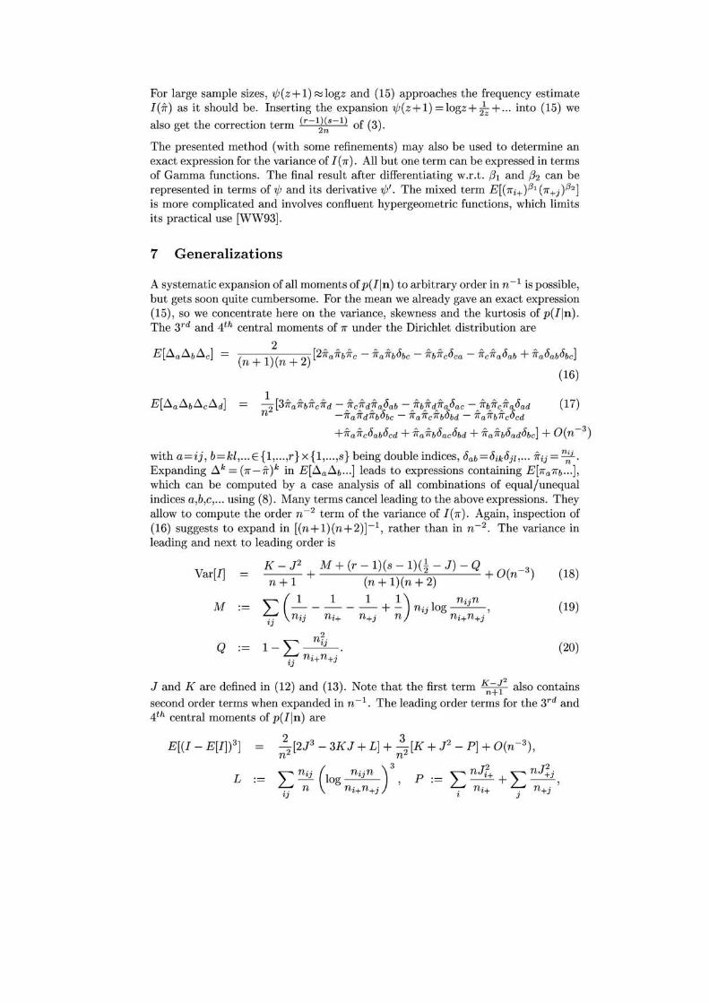
For large sample sizes, 'Ij;(z + 1) ~ logz and (15) approaches the frequency estimate I(7r) as it should be. Inserting the expansion 'Ij;(z + 1) = logz + 2\ + ... into (15) we also get the correction term (r - 11~s - 1) of (3).

The presented method (with some refinements) may also be used to determine an exact expression for the variance of I(7f). All but one term can be expressed in terms of Gamma functions. The final result after differentiating w.r.t. (31 and (32 can be represented in terms of 'Ij; and its derivative 'Ij;' . The mixed term E[( 7fi+ )131 (7f +j )132] is more complicated and involves confluent hypergeometric functions, which limits its practical use [WW93] .

7 Generalizations

A systematic expansion of all moments of p(Iln) to arbitrary order in n -1 is possible, but gets soon quite cumbersome. For the mean we already gave an exact expression (15), so we concentrate here on the variance, skewness and the kurtosis of p(Iln). The 3rd and 4th central moments of 7f under the Dirichlet distribution are

( )2( ) [27ra7rb7rc - 7ra7rbc5bc - 7rb7rcc5ca - 7rc7rac5ab + 7rac5abc5bc] n+l n+2

(16)

~2 [37ra7rb7rc7rd - jrc!!d!!a c5ab - A7rbjrdA7rac5ac - A7rbA7rcA7rac5ad (17) -7fa7fd7fbc5bc - 7fa7fc7fbc5bd - 7fa7fb7fcc5cd

+7ra7rcc5abc5cd + 7ra7rbc5acc5bd + 7ra7rbc5adc5bc] + O(n-3)

with a=ij, b= kl, ... E {1, ... ,r} x {1, ... ,8} being double indices, c5ab =c5ik c5jl , ... 7rij = n~j •

Expanding D..k = (7f_7r)k in E[D..aD..b ... ] leads to expressions containing E[7fa7fb ... ], which can be computed by a case analysis of all combinations of equal/unequal indices a,b,c, ... using (8). Many terms cancel leading to the above expressions. They allow to compute the order n-2 term of the variance of I(7f). Again, inspection of (16) suggests to expand in [(n+l)(n+2)]-1, rather than in n-2 . The variance in leading and next to leading order is

Var[I] K - J2 + M + (r - 1)(8 - 1)(~ - J) - Q + O(n- 3) n + 1 (n + l)(n + 2)

(18)

M L (~- _1 _ _ _ 1_ +~) nij log nijn , ij nij ni+ n+j n ni+n+j

(19)

Q 2

l-L~· ij ni+n+j

(20)

J and K are defined in (12) and (13). Note that the first term ~+f also contains

second order terms when expanded in n -1. The leading order terms for the 3rd and 4th central moments of p(Iln) are

L .-

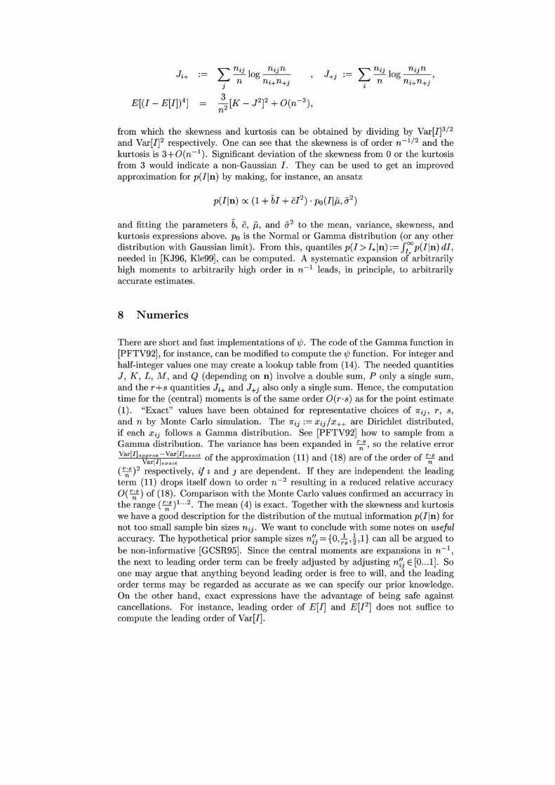
'""" nij I nij n ~- og---

j n ni+n+j

32 [K - J 2F + O(n- 3 ), n

from which the skewness and kurtosis can be obtained by dividing by Var[Ij3/2 and Var[IF respectively. One can see that the skewness is of order n-1/ 2 and the kurtosis is 3 + 0 (n - 1). Significant deviation of the skewness from a or the kurtosis from 3 would indicate a non-Gaussian I. They can be used to get an improved approximation for p(Iln) by making, for instance, an ansatz

and fitting the parameters b, c, jJ" and (j-2 to the mean, variance, skewness, and kurtosis expressions above. Po is the Normal or Gamma distribution (or any other distribution with Gaussian limit). From this, quantiles p(I>I*ln):= fI:'p(Iln) dI, needed in [KJ96, Kle99], can be computed. A systematic expansion of arbitrarily high moments to arbitrarily high order in n-1 leads, in principle, to arbitrarily accurate estimates.

8 Numerics

There are short and fast implementations of'if;. The code of the Gamma function in [PFTV92], for instance, can be modified to compute the 'if; function. For integer and half-integer values one may create a lookup table from (14) . The needed quantities J, K, L, M, and Q (depending on n) involve a double sum, P only a single sum, and the r+s quantities Ji+ and J+j also only a single sum. Hence, the computation time for the (central) moments is of the same order O(r·s) as for the point estimate (1). "Exact" values have been obtained for representative choices of 7rij, r, s, and n by Monte Carlo simulation. The 7rij := Xij / x++ are Dirichlet distributed, if each Xij follows a Gamma distribution. See [PFTV92] how to sample from a Gamma distribution. The variance has been expanded in T~S, so the relative error Var [I]app"o.-Var[I] .. act of the approximation (11) and (18) are of the order of T'S and

Var[Il e• act n

(T~S)2 respectively, if z and J are dependent. If they are independent the leading term (11) drops itself down to order n -2 resulting in a reduced relative accuracy O( T~S) of (18). Comparison with the Monte Carlo values confirmed an accurracy in the range (T~S)1...2. The mean (4) is exact. Together with the skewness and kurtosis we have a good description for the distribution of the mutual information p(Iln) for not too small sample bin sizes nij' We want to conclude with some notes on useful accuracy. The hypothetical prior sample sizes n~j = {a, -!S' ~,1} can all be argued to be non-informative [GCSR95]. Since the central moments are expansions in n-1 ,

the next to leading order term can be freely adjusted by adjusting n~j E [0 ... 1]. So one may argue that anything beyond leading order is free to will, and the leading order terms may be regarded as accurate as we can specify our prior knowledge. On the other hand, exact expressions have the advantage of being safe against cancellations. For instance, leading order of E[I] and E[I2] does not suffice to compute the leading order of Var[I].

Acknowledgements

I want to thank Ivo Kwee for valuable discussions and Marco Zaffalon for encour­aging me to investigate this topic. This work was supported by SNF grant 2000-61847.00 to Jiirgen Schmidhuber.

References

[AS74]

[Bra99]

[Bun96]

[CT91]

M. Abramowitz and 1. A. Stegun, editors. Handbook of mathematical functions. Dover publications, inc., 1974.

M. Brand. Structure learning in conditional probability models via an entropic prior and parameter extinction. N eural Computation, 11(5):1155- 1182, 1999.

W. Buntine. A guide to the literature on learning probabilistic networks from data. IEEE Transactions on Knowledge and Data Engineering, 8:195- 210, 1996.

T. M. Cover and J. A. Thomas. Elements of Information Theory. Wiley Series in Telecommunications. John Wiley & Sons, New York, NY, USA, 1991.

[GCSR95] A. Gelman, J. B. Carlin, H. S. Stern, and D. B. Rubin. Bayesian Data Analysis. Chapman, 1995.

[Hec98] D. Heckerman. A tutorial on learning with Bayesian networks. Learnig in Graphical Models, pages 301-354, 1998.

[KJ96] G. D. Kleiter and R. Jirousek. Learning Bayesian networks under the control of mutual information. Proceedings of the 6th International Conference on Information Processing and Management of Uncertainty in Knowledge-Based Systems (IPMU-1996), pages 985- 990, 1996.

[Kle99] G. D. Kleiter. The posterior probability of Bayes nets with strong dependences. Soft Computing, 3:162- 173, 1999.

[PFTV92] W. H. Press, B. P. Flannery, S. A. Teukolsky, and W. T. Vetterling. Numerical R ecipes in C: The Art of Scientific Computing. Cambridge University Press, Cambridge, second edition, 1992.

[SooOO] E. S. Soofi. Principal information theoretic approaches. Journal of the Ameri­can Statistical Association, 95:1349- 1353, 2000.

[WW93] D. R. Wolf and D. H. Wolpert. Estimating functions of distributions from A finite set of samples, part 2: Bayes estimators for mutual information, chi­squared, covariance and other statistics. Technical Report LANL-LA-UR-93-833, Los Alamos National Laboratory, 1993. Also Santa Fe Insitute report SFI-TR-93-07 -047.