Distribution Network Redesign for Marketing … Shang, Tuba Pinar Yildirim, Pandu Tadikamalla, Vikas Mittal, & Lawrence H. Brown Distribution Network Redesign for Marketing Competitiveness

146Journal of MarketingVol. 73 (March 2009), 146–163

© 2009, American Marketing AssociationISSN: 0022-2429 (print), 1547-7185 (electronic)

Jennifer Shang, Tuba Pinar Yildirim, Pandu Tadikamalla, Vikas Mittal, &Lawrence H. Brown

Distribution Network Redesign forMarketing Competitiveness

This article reports on a marketing initiative at a pharmaceutical company to redesign its distribution network.Distribution affects a firm’s cost and customer satisfaction and drives profitability. Using a nonlinear mixed-integerprogramming model, the authors develop a distribution network with a dual emphasis on minimizing the totaldistribution costs and improving the customer service levels. Specifically, they address the following issues: They(1) determine the optimal number of regional distribution centers the firm should operate with, (2) identify where inthe United States the firm should locate these distribution centers, (3) allocate each retailer/customer distributioncenter to an appropriate regional distribution center, and (4) determine the total transportation costs and servicelevel for each case. Finally, they conduct a sensitivity analysis to determine the impact of changes in problemparameters on the optimality of the proposed model. This marketing initiative at the studied firm reduced the totaldistribution costs by $1.99 million (6%) per year, while increasing the customer on-time delivery from 61.41% to86.2%, an improvement of 40.4%.

Keywords: location theory, optimization, decision calculus, network design, supply chain model

Jennifer Shang is Associate Professor of Business Administration (e-mail:[email protected]), Tuba Pinar Yildirim is a doctoral candidate (e-mail:[email protected]), and Pandu Tadikamalla is Professor of BusinessAdministration (e-mail: [email protected]), Katz Graduate School ofBusiness, University of Pittsburgh. Vikas Mittal is J. Hugh Liedtke Profes-sor of Marketing, Jones Graduate School of Management, Rice University(e-mail: [email protected]). Lawrence Brown is Vice President of CustomerSupply and Planning, GlaxoSmithKline Company (e-mail: [email protected]).

As the service element of customer experiencesbecomes more important, location and conveniencehave emerged as major factors in consumer deci-

sions for products and services (e.g., Chan, Padmanabhan,and Seetharaman 2007; Devlin and Gerrard 2004; Ghoshand Craig 1986; Mulhern 1997; Thelen and Woodside1997). As Ghosh and Craig (1983, p. 56) argue,

A good location provides the firm with strategic advan-tages that competition may find difficult to overcome.While other marketing mix elements may be easilychanged in response to a changing environment, storelocations represent long-term investments that can bechanged only at a considerable cost.

Over the past decade, retailers have attempted to man-age their store locations strategically to reach more andmore consumers (Langston, Clarke, and Clarke 1997). Asthe number of retail outlets has increased, manufacturershave responded by modifying their distribution network toeliminate stockouts, minimize late deliveries, and reducesupply costs by changing shipping routes, relocating distri-bution centers, and reconfiguring warehouses (Deveci-Kocakoc and Sen 2006). Within the marketing discipline,although research on retail locations has been conducted

by many scholars (e.g., Ghosh and Craig 1983, 1986; Kuo,Chi, and Kao 2002; Mahajan, Sharma, and Kerin 1988;Pinkse, Slade, and Brett 2002), there is a dearth of researchon how manufacturers can design their distribution networkin response to retailer location networks. Korpela andLehmusvaara (1999) empirically study retail clients of amanufacturer and find that factors such as delivery time,quality, total cost, and ability to meet consumers’ urgent/special needs are key drivers that affect retailers’ decisionsto carry the manufacturer’s products. These factors shouldguide decisions about distribution centers and warehousinglocations.

Rust and colleagues (2004) highlight the importance ofefficiency in marketing systems to make marketing morefinancially accountable to top management. Using the non-linear mixed-integer programming approach, we develop adistribution network that not only improves efficiency byminimizing the total distribution costs but also improvescustomer service levels. We illustrate our approach in thecontext of a global pharmaceutical firm in which the mar-keting department, responding to the needs of the retailersand top management, launched an initiative aimed atreengineering the firm’s distribution network.

The model we propose herein addresses the followingissues: (1) determining the “optimal” number of regionaldistribution centers (RDCs) the manufacturing firm shouldoperate with, (2) identifying where in the United States thefirm should locate these distribution centers, (3) allocatingeach of the retailer/customer distribution centers (CDCs) toan appropriate warehouse, and (4) determining the totaltransportation costs and service level for the optimal sce-nario, as well as other scenarios. A sensitivity analysisexamines the impact of changes in model parameters on theoptimality of the proposed model. Finally, to understand

Distribution Network Redesign / 147

the quality of our methodology, we compare the solutionapproach with two other heuristics. This marketing initia-tive was able to reduce the total distribution costs of thestudied firm (GlaxoSmithKline [GSK]) by $1.99 million(6%) per year and to increase on-time delivery from61.41% to 86.2%, an improvement of 40.4%.

Answering the call of Rust and colleagues (2004, p. 84)that marketing’s contribution should specifically focus on“core business processes and efficient supply chain pro-cesses,” we show how to improve the efficiency and effec-tiveness of distribution systems simultaneously. In doing so,we show the interdependency of retail strategy and distribu-tion strategy in terms of location analysis. Despite a largefocus on retail stores’ location selections (e.g., Devlin andGerrard 2004; Ghosh and Craig 1986; Mulhern 1997), theirinterdependence on the distribution network has not beenexamined. Yet successful retailers, such as Wal-Mart andTarget, demonstrate the need for incorporating distributionstrategy for marketing success. Finally, we show how inputfrom marketing managers can be gainfully used in distribu-tion design. This not only illustrates the concept of decisioncalculus (Chakravarti, Mitchell, and Staelin 1979; Little2004) but also shows how the decision calculus approachdeveloped in marketing can be applied more broadly. Forexample, we obtained managerial input on problem formu-lation, along with the various parameters of the distributionnetwork.

We organize the rest of the article as follows: We beginwith a review of the distribution network design from mar-keting and operations management literature regarding thestructure of a firm’s supply chain. We provide details of thegeneric network design model and its analysis in the “Prob-lem Formulation and Methodology” section. Then, weapply the generic model to GSK. We follow this with theresults of the application, conduct a sensitivity analysis ofthe recommended solution methodology, and compare theperformance of our approach with other heuristics. Finally,we provide a summary of findings and note the limitationsof this research.

Literature ReviewMotivated by the importance of store location and cus-tomer convenience as key elements of marketing strategy,scholars have developed models to guide optimal locationdecisions for retailers and service providers (Bucklin 1967;Cox 1959; Ghosh and McLafferty 1982; Mulhern 1997).Early models used regression analysis to determine storelocations (Lord and Lynds 1981), while later models alsoincorporated insights from game theory and decision theory (e.g., Davis 2006; Ghosh and Craig 1983, 1986).More recently, Chan, Padmanabhan, and Seetharaman(2007) estimated an econometric model that incorporatesthe geographic location of retailers and models the pricecompetition among them to determine consumer policyimplications. Empirically, models have been developed toincorporate the spatial variability in customer tastes whendetermining store locations (Donthu and Rust 1989; Mittal,Kamakura, and Govind 2004; Rust and Donthu 1995).Thus, in marketing, there is a rich tradition of examining

retail locations from the retailer’s or customer’s perspective.However, the location choices made by manufacturers tosupport retailer networks have received relatively littleattention in the marketing literature. Yet it is well knownthat manufacturer decisions can have a critical effect on themarketing success of downstream retailer partners (Iyer andBergen 1997; Kadiyali, Chintagunta, and Vilcassim 2000;Murry and Heide 1998). This is the focus of the currentresearch.

The field of location analysis has been extensively stud-ied (for a review, see Brandeau and Chiu 1989; Daskin1995). The location and allocation decisions in supply chainnetwork design, including the choice of the number, site,and capacity of facilities, as well as assigning customers tothese facilities, have significant long-term impacts on theefficiency of the network. Model formulations and solutionalgorithms that address these issues vary widely in terms offundamental assumptions, mathematical complexity, andcomputational performance. We review key developmentsin this literature.

Design of a Distribution Network

Research in location–allocation often focuses on cost reduc-tion, demand capture, equitable service supply, and fastresponse time. Baumol and Wolfe (1958) were the first todescribe a distribution model. Geoffrion and Graves (1974)proposed a multicommodity supply chain design model tooptimize product flows from plants to RDCs, RDCs toCDCs, and CDCs to final customers. Work by Brown,Graves, and Honczarenko (1987), Cohen and Lee (1988),and Arntzen and colleagues (1995) models the location andallocation problem as a mixed-integer linear programmingproblem and provides an efficient heuristic algorithm tosolve large-scale problems.

Geoffrion and Powers (1995) examine the evolution ofthe strategic distribution system design since 1970. Reviewsof distribution models with emphasis on supply chain mod-els can also be found in the work of Vidal and Goetschalckx(1997) and Beamon (1998). In a review, Erenguc, Simpson,and Vakharia (1999) emphasize the importance of opera-tional issues, such as lead times in making location/allocation decisions. Melkote and Daskin’s (2001) modelinvolves both fixed and arc/variable costs and focuses onthe number, location, capacity, and size of warehouses to beset up to maximize profits. However, in this model, manu-facturing facilities are not taken into account. Eskigun andcolleagues (2005) study the distribution management issuefaced by a large-scale automotive firm. Finally, Saourirajan,Ozsen, and Uzsoy (2007) focus on stochastic issues andincorporate lead time and safety stock into their model.

The problem we encountered at GSK required address-ing four main questions: (1) How many distribution centersshould be opened? (2) Where should the distribution centersbe located? (3) What should the capacity of each distribu-tion center be? and (4) How should customers be allocatedto distribution centers? Table 1 summarizes the literaturethat is most relevant to our problem. Our ability to addressall four questions in a unified framework provides animportant contribution to the literature.

148 / Journal of Marketing, March 2009

TABLE 1Distribution Management Literature Most Relevant to the Studied Problem

MethodQuestions Addressed Technique Strength Weakness

Amiri (2006) 1, 3, 4 Lagrangian heuristic Include plants andwarehouse decision

Single product type

Brown, Graves, andHonczarenko (1987)

1, 4 Goal decomposition Where and how much toproduce, where to ship

from

Focus on solution time

Eskigun et al. (2005) 1, 3, 4 Lagrangian heuristic Consider lead time,capacity

Single product type:vehicle

Jayaraman and Ross(2003)

1, 3, 4 Mixed-integerprogramming, simulated

annealing

Include cross-docking Need to know potentialcross-docks and

warehouses

Melkote and Daskin (2001) 1 Mixed-integerprogramming

Consider capacity Demand travels to facilities

Moon and Chaudhry(1984)

2 Integer programming Introduce various distance-constrained problem

Focus on location only

Swersey and Thakur(1995)

1, 3 Integer programming, setcovering problem

Identify location Single stage, nodistribution decision

involved

Notes: The numbers in Column 2 correspond to the following questions: (1) how many distribution centers, (2) where to locate, (3) what capac-ity, and (4) how to allocate customers.

The Continuous Location Problem

The main distinction between our model and the traditionalsupply chain design is that ours is a “continuous model”rather than a traditional discrete location model. Further-more, we do not begin with a preset network design. Ourcontinuous model assumes that facilities (e.g., RDCs) canbe represented by any point in the Euclidean plane, andtravel distances in the mathematical model are calculated byeither the Euclidean metric or the Manhattan metric. Con-versely, the traditional discrete models, which form the bulkof prior research, assume that facilities can be located onlyat specific and limited numbers of potential sites. Becauseof its relevance to our research, we review the continuousmodel next.

The core of the continuous location problem rests on theWeber problem (Wesolowsky 1993). It determines the coor-dinates of a single facility, such that the sum of the(weighted) distances wl × dl(x, y) from the facility to thecustomer at (al, bl) is minimized—that is, MinΣlwl × dl(x,y). Among the many measures proposed to determine theproximity between two points on a plane, the Euclidean dis-tance is the simplest and easiest to implement (Anderberg1973; Gower 1985). For a facility at (x, y) and customer l at(al, bl), the Euclidean distance is computed as dl(x, y) =

The coordinates of the city in which acustomer resides can be uniquely identified by the zip code,which matches a specific city.

An extension of the problem that allows for multiplefacilities and allocates demands to facilities is the multi-

( ) ( ) .x a y b− + −l l2 2

source Weber problem (MWP). Locating multiple facilitiessimultaneously in a plane to minimize the total transporta-tion cost and to satisfy the demand for many users is a non-deterministic polynomial-time hard problem (Klose andDrexl 2005), and it can be modeled as a nonlinear mixed-integer program as follows:

subject to for each customer l, where zkl ={0, 1} and zkl equals 1 if customer l is assigned to facility k,and x, y are continuous variables.

The main difficulty in solving the MWP arises becausethe objective function is not convex (Cooper 1967) and canhave a large number of local minima. Heuristics are neededto solve large problems and to provide good initial solutionsfor exact algorithms. In the MWP, it is assumed that thenumber of new facilities to be located (k) is given. In prac-tice, however, determining the number of facilities is one ofthe main questions that needs to be answered. Rosing(1992) and Du Merle and colleagues (1999) reformulate thepreceding MWP model as a set partitioning problem anduse the column generation approach to solve the linear pro-gramming relaxed version of the problem. Other variantsand extensions of the MWP can be found in Klamroth(2001). To date, all continuous location problems discussedin the literature have been single echelon (i.e., they focusonly on one level of supply and demand). However, multi-echelon supply chains (i.e., various levels in distribution

ΣkK

kz= =1 1l

Min w d x y zk

kL

k k kl

l

l l

==∑∑

11

( ) ,,


network, including suppliers, manufacturers, distributors,retailers, and customers) are needed to carry out the goalsof an organization such as GSK. Thus, we develop a modelfor multiechelon supply chain network design.

Problem Formulation andMethodology

A supply chain network should satisfy customers’ demandssimultaneously at a desired service level and at the lowestpossible cost. To do this, we propose a generic modelingframework that is flexible and general enough to incorpo-rate various constraints such that important location andallocation conditions are taken into account. We call ourapproach the “continuous supply chain design” (CSCD)problem. This approach results in a realistic nonlinearmixed-integer programming model.

The CSCD Model

The following CSCD model is an extension of the MWP tothe multiechelon setting. It focuses on the decisions of loca-tion and allocation of RDCs. We describe the notation in theAppendix and formulate the CSCD model as follows:

subject to

(5) ukl ≤ zk ∀l;

(8) ukl, zk = {0, 1} ∀k, l;

(9) sijk, tikl ≥ 0 ∀j, k, l;

(10) xk, yk are continuous variables.

The CSCD is a large-scale nonlinear mixed-integer pro-gramming model. The objective function, Equation 1, mini-mizes the cost of transportation between plants and RDCs,

( )6 t D

t

tw

ikk

i

iki

ikki

k

l l

l

l

l

l

l∑

∑∑∑∑∑

= ∀

=

i, ;

(7) ∀∀k;

( )

( ) ,

2 1

3

u ;

;

(4)

kk

jijk ikl k

k

s t u i k

l

l

l

l∑

∑

= ∀

= ∀Σ

Σzz Kk ≤ ;

( ) ( ),1111

Min d x y si

I

k

K

j

J

j k k ig × ×===

∑∑∑ jjk

k k ik ki

I

k

K

h d x y t u+ × × ×===

∑∑ l ( ), l l

l 1111 1

L

k

k

k kf w z∑ ∑+ ×=

( ) ,

the cost of shipping between RDCs and CDCs, and thecosts of opening and operating RDCs. Constraints in Equa-tion 2 are single-sourcing constraints that restrict a cus-tomer’s demand for any commodity to be served by a singleRDC. Constraints in Equation 3 ensure that all productsshipped to an RDC will be shipped to CDCs. Constraints inEquation 4 specify the maximum number of RDCs to open.Constraints in Equation 5 allow CDCs to be assigned to theopened RDCs only. Constraints in Equation 6 ensure that allcustomer demands are satisfied. Constraints in Equation 7determine the relative size of warehouse k. Constraints inEquation 8 ensure that ukl and zk are binary. Variables sijkand tikl are nonnegative, as required in the constraints inEquation 9. The coordinates (xk, yk) take any positive ornegative number without restriction, as the constraints inEquation 10 show.

The CSCD model simultaneously identifies the appro-priate sites for RDCs, allocates each CDC to a specificRDC, determines the ideal number of RDCs, determines the size of each RDC, and minimizes the total distributionnetwork costs. In addition to the multiechelon continuousnature, the proposed CSCD model differs considerablyfrom the traditional location and allocation models in sev-eral ways. First, information about warehouse capacity(size) is not required, which is different from previous mod-els in the literature (e.g., Amiri 2006; Brown, Graves, andHonczarenko 1987; Eskigun et al. 2005; Jayaraman andRoss 2003; Melkote and Daskin 2001). Note that the size ofan RDC is proportional to the total demand assigned to thatspecific site, and the costs of the RDCs are estimated on thebasis of size. In other words, both the size and the locationof any RDC depend on the solution of the model and are notprovided as parameters. Managerially, this implies that theleasing and operating costs depend on the size of the RDCsopened. Second, no potential RDC locations need to beidentified before solving the model, which is different frommost of the location selection models in the literature (e.g.,Moon and Chaudhry 1984; Swersey and Thakur 1995).Third, prior models have used constant shipping costs tocompute the total transportation costs (e.g., Amiri 2006;Elhedhli and Goffin 2005; Erlenkotter 1978; Shen 2005). Inthis study, transportation cost (parameters g and h in theCSCD model) is a function of the diesel price, distance,weight, line-haul costs, and fuel surcharge, as we discuss inthe subsequent subsections. Incorporating these factorsmakes the model more realistic because these are issues thatmanagement must address on a day-to-day basis.

The complexity involved in making the problem formu-lation more realistic implies that the problem also becomesmore difficult to solve optimally. To the best of our knowl-edge, the CSCD model in this study is the first to integrate acontinuous location problem and a comprehensive multi-echelon supply chain network design problem, both ofwhich are classified as nondeterministic polynomial-timehard problems. Problems in this category cannot be opti-mally solved in a reasonable amount of time (polynomialtime), often taking days, weeks, and more, depending onthe scale of the problem. As a consequence, exact optimalsolution methods are restricted to small-scale problems, and


such problems often end up being unrealistic. Thus, effec-tive heuristic algorithms are developed to provide near-optimal solutions within minutes. Next, we describe howwe solve the CSCD problem using a heuristic.

Solution Approach

Many heuristics of different accuracy and speed have beensuggested to solve the location and allocation problem.Most problems are solved by modern heuristic procedures,which do not guarantee an optimal solution. Our goal is notto pursue the exact mathematical optimum but rather tosolve the problem efficiently and realistically. In otherwords, we want an algorithm that can generate a relativelygood solution within a reasonable amount of time (i.e., min-utes or hours, not months or years). The genetic algorithmin Evolutionary Solver can serve such a purpose. The Evo-lutionary Solver (Ashlock 2005) is a Microsoft Excel add-intool found in Premium Solver (Frontline Systems 2007).

The genetic algorithm approach, introduced by Holland(1975), is a global search heuristic procedure that incorpo-rates processes inspired by evolution ideas in biology, suchas initiation, selection, reproduction (crossover and muta-tion), and termination (see Figure 1). A series of steps areused to solve the CSCD model. First, the genetic algorithmstarts by randomly generating a large set of candidates to

form initial solutions, called a “population,” and then evalu-ates the fitness (quality) of each individual candidate (i.e.,solution) in the population. Whether an individual solutionis fit depends on whether it can satisfy all constraints andthe solution quality. Second, the genetic algorithm selectstwo best-ranking individual solutions to reproduce throughcrossover and mutation (genetic operations) and to givebirth to offspring (i.e., pairs of the existing population tocreate offspring for the next generation). Third, the geneticalgorithm evaluates the fitness of each offspring, replacingthe worst-ranked part of population with the best offspring.Therefore, the population evolves and becomes more fit.Fourth, the genetic algorithm occasionally makes a randomchange by substituting a member in the population by a ran-dom value. Such a mutation can create offspring that are farremoved from the rest of the population to avoid beingstuck at a local optimum. Fifth, the genetic algorithm con-tinues creating new generations until no improvementsoccur in several successive generations. The algorithm ter-minates, and the best result found becomes the solution.

In applying the genetic algorithm in EvolutionarySolver, we use large values in maximum subproblems andmaximum feasible solutions to extend the search. Increas-ing the population size and/or mutation rate helps improvewith searches that were trapped in local optimum. Con-

FIGURE 1The Flowchart of Genetic Algorithm


FIGURE 2Distribution Network of GSK

versely, decreasing the tolerance and/or increasing themaximum time without improvement allows for a longersearch and a chance to improve results. All these are criticaluser inputs to the software program to help detect a bettersolution.

Although the genetic algorithm does not guarantee anoptimal solution, Wen and Iwamura (2008) find that it islikely for the genetic algorithm to end up with a solutionthat is close to optimal. To improve the chance of obtainingthe best solution, a standard optimization model can be run,starting with the final solution obtained by the EvolutionarySolver, to seek an opportunity for enhancing the solutionquality.

Applying the CSCD Model to GSKA real-life case study at GSK provides the setting for imple-menting our model. The CSCD model has successfully han-dled the problem, and the company’s marketing and logis-tics department recognizes the validity of the results.Because of confidentiality concerns, some numerical resultsreported here are disguised.

The Distribution Network of GSK

GlaxoSmithKline’s supply chain network consists of sup-pliers, manufacturers, warehouses, and retail distributionchannels, which are synchronized to acquire raw materials,produce finished goods, and distribute products to ware-houses and retailers. Currently, most products are producedby four manufacturing plants in the United States and morethan 30 contractors around the world. They manufacture 60brands and more than 1200 different items, representingapproximately 4 billion packs per year. Together with twocopacking facilities, they form the supplier network of thecompany’s consumer health care products. The firm hasfour RDCs in the United States to ship its products to morethan 400 retail accounts, each of which has multiple CDCs.In all, there are 25,000 “ship-to” locations (i.e., retailstores). Annually, more than 80,000 customer orders arehandled, and 20 million cases of products are shipped. Fig-ure 2 provides the direction of the inventory flow. The loca-tions of current manufacturing plants and RDCs appear inFigure 3.

As Figure 3 shows, GSK currently has four RDCslocated in Fountain Inn, S.C.; Memphis, Tenn.; Hanover,Penn.; and Fresno, Calif. These RDCs receive inboundshipments from manufacturing facilities located in Aiken,S.C.; Clifton, N.J.; Memphis, Tenn.; and St. Louis; Mo. Noproducts are stored in the manufacturing facilities. If anRDC is short of a product, another RDC is allowed to shareinventory and ship to the RDC in need. However, manage-ment has deemed that such an activity wastes resources andthus is strongly discouraged. Therefore, interwarehouseshipping is avoided and should not be considered in ourmodel.

After an RDC receives products, it ships them to thecorresponding CDCs. When the CDC receives the products,the customer takes possession and title of the goods. TheseCDCs are spread around the United States, with moreCDCs on the East Coast than the West Coast. The existing

distribution network of GSK has been employed for morethan a decade and is a result of incremental changes as thecompany has grown. A major opportunity for improvementof the distribution network arose when the current leases onsome RDCs were due for expiration and renewal. The firmhad the option either to renew some of the leases or to lookfor alternative sites if necessary. In addition, managementwas concerned with the rising costs of fuel, a key cost fac-tor. During the second half of 2005, diesel prices rose46.5%, from an average of $2.15 to $3.15 per gallon, andthey reached $3.80 in March 2007. The executives man-dated that any distribution network design include the costsof energy as a key decision factor. In other words, the firmwanted to relocate its RDCs such that a potential change inthe environment, such as customer demand and dieselprices, would have the smallest possible impact on the dis-tribution costs.

Determining the Number, Sites, and Capacities ofthe RDCs

We obtain the model solution with the Evolutionary Solver,which determines the geographical coordinates of RDCs,which are then converted into zip codes and used to identifythe corresponding cities. Specifically, the CSCD modeldetermined that the optimal warehouse (RDC) coordinateswere (33.5, –96.9), (37.1, –118.6), (33.4, –83.8), (41.6,–87.9), and (40.2, –76.3). These coordinates correspondedto zip codes 76233, 93513, 31085, 60441, and 17545, repre-senting five cities: Collinsville, Tex. (RDC 1); Big Pine,Calif. (RDC 2); Shady Dale, Ga. (RDC 3); Lockport, Ill.(RDC 4); and Manheim, Penn. (RDC 5). The model alsoassigned each CDC to one of these RDC locations to mini-mize the total costs. Many of GSK’s retailers have multipleCDCs that are geographically dispersed throughout theUnited States; therefore, different CDCs for the sameretailer (e.g., Wal-Mart) can be served by different RDCs.

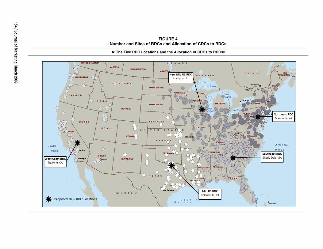
We summarize the solution to GSK’s RDC location andallocation problem in Table 2 and map this onto U.S. citiesin Figure 4. In Table 2, the percentages show the relative

152/ Journal of M

arketing,March 2009

FIGURE 3RDCs and Manufacturing Plants for GSK


TABLE 2The Results of Applying the CSCD Model to the

GSK Data

Chosen City, StateZip

CodeRelative Size of

Warehouse Capacity

Collinsville, Tex. 76233 21%Big Pine, Calif. 93513 21%Shady Dale, Ga. 31085 24%Lockport, Ill. 60441 19%Manheim, Penn. 17545 16%

size of each warehouse. Each value is derived from Equa-tion 7. Figure 4, Panel A, shows the CDCs that are to beserved by each proposed RDC on a U.S. map. Circles of thesame shade are CDC locations that are assigned to the sameRDC. Figure 4, Panel B, shows the old and new RDCs.

Deriving the Unit Transportation Costs on theBasis of the Cost Structure of Freight

To understand the cost structure of freight for this firm, it isimportant to distinguish between full-truckload (TL) andless-than-truckload (LTL) shipping. By TL, we refer toshipments of a full truckload to obtain economies of scale,and by LTL we refer to the shipments with a relativelysmall freight that does not fill the truck. Truck drivers areexpected to transport freight at an average rate of 47 milesper hour (this factors in traffic jams and queues at intersec-tions) all the way to destination. The advantage of TL carri-ers is that the freight is never handled en route, giving amore predictable delivery time, whereas an LTL shipmentmay be transported on several different trailers to achievehigher volume efficiency. The main advantage of LTL ship-ment is that it is much cheaper than TL. Many, if not all,carriers view themselves as either primarily LTL or primar-ily TL carriers. GlaxoSmithKline’s manufacturers use TL toship from plants to RDCs to ensure efficiency and use LTLto ship from RDCs to CDCs to customize clients’ needs.

Thus far, researchers (e.g., Amiri 2006; Elhedhli andGoffin 2005; Shen 2005) working on location and alloca-tion problems have used average unit shipping costs tocompute the total transportation costs. However, in reality,freight costs differ significantly between TL and LTL ship-ments. Equations 11–15 distinguish the TL and LTL costsand identify the underlying transportation cost structure forGSK.

When the quantities are shipped as containerized intruckloads or when the transportation cost structure chargesa truckload minimum for partial quantities, product distri-bution cost mainly becomes a function of the distance trav-eled. However, under a partial-load price structure, it iscommon to express the pricing in terms of load distances,such as ton–mile, where a ton–mile is the amount of trans-portation activity to move a ton of material over a distanceof one mile. To keep our model general, we express thetransportation activity in load distances because the puredistance-based approach is a special case of the generalmodel when the minimum charged quantities are intruckloads.

For both TL and LTL types of transport, fuel surchargeand line-haul charges are the two main costs. The totalfreight cost can be formulated as follows:

(11) Total transportation cost = Demurrage + Line-haul cost

+ Fuel surcharge.

All the information needed for Equation 11 is obtained byGSK in advance. Plugging these data into Equation 11 givesthe LTL and TL freight costs, which correspond to g and hin the CSCD model. The demurrage in Equation 11 is thecost imposed as compensation for the detention of a carriertaking longer than the normal time needed to load andunload a truck. Line-haul costs are basic charges for long-distance moves, which are usually calculated on the basis ofmileage and weight of the shipment. Fuel surcharge is anadditional per-shipment fee that carriers impose when fuelprices are above predefined levels.

Using the historical shipment data provided by GSKand the characteristics of customer orders, we express line-haul costs as regression models (see Equations 12 and 13).For the LTL regression equation, the independent variables,distance (p < .0001) and weight (p < .0001), were both sta-tistically significant. The model was adequate with a highR-square value (98.2%). Conversely, for the TL regressionequation, only distance was significant (p < .0001), and themodel was able to account for a high portion of variation(R2 = 91.3%).

(12) LTL: Line-haul = $12.79 + .06 (Distance)

+ .056 (Weight), and

(13) TL: Line-haul = $399.48 + 1.0268 (Distance).

In these equations, we do not include additional variables,such as size, type, and volume of customer order, becausewe found them to be insignificant in determining the line-haul costs. In both equations, distance is statistically signifi-cant, but weight is significant only in the LTL situation. Weexpect weight to be insignificant in the TL equation becausethe truck is always full, and in general, fully loaded trucksweigh similarly in this case.

In addition to line-haul costs, carriers also impose a fuelsurcharge cost. Using the Department of Energy’s DieselFuel Index, we estimate the fuel surcharge costs for LTLand TL in Equations 14 and 15:

(14) LTL: Fuel surcharge = ({[.3(Diesel price – 1.15)/.05]

+ .7}/100) × Line-haul cost, and

(15) TL: Fuel surcharge = (.2 × Diesel price – .2298)

× Miles traveled.

Equation 14 shows that fuel surcharge is the product of thesurcharge rate and the line-haul cost for LTL shipment. Thesurcharge rate in Equation 14 ({[.3(Diesel price – 1.15)/.05] + .7}/100) reflects that for each $.05 increase over$1.15 in the diesel price, the fuel surcharge will increase by.3% of the line-haul cost. In the calculation, this is roundeddown for convenience. For TL, the diesel price and miles

154/ Journal of M

arketing,March 2009

FIGURE 4Number and Sites of RDCs and Allocation of CDCs to RDCs

A: The Five RDC Locations and the Allocation of CDCs to RDCsa


FIGURE 4Continued

B: Previous RDC Locations and the New Five-RDC Solution Locationsb

aSmall circular dots represent existing CDC locations in the United States, and stars with city names and state represent the proposed new five RDC locations.bRelative capacities of the plants are as follows: Collinsville, Tex. (21%); Big Pine, Calif. (21%); Shady Dale, Ga. (24%); Lockport, Ill. (19%); and Manheim, Penn. (16%).


traveled define the fuel surcharge; again, weight is not animportant factor.

The parameters estimated in Equations 11–15 help man-agement better understand the relationship among the com-ponents of transportation cost. GlaxoSmithKline can plugin these components and quickly and approximately esti-mate the transportation costs for each of the items it shipsannually.

The cost function of RDCs is a function of the size ofthe warehouse: 676 × (100 × Size)1⁄2, which suggests thatthere are economies of scale. If we combine the transporta-tion costs of Equation 11 with warehouse cost function, thetotal distribution network costs for CSCD can be derived.

Total Distribution Network Costs and ServiceLevel

Although having fewer RDCs lowers the fixed and operat-ing costs associated with the warehouse management, itincreases both the inbound and the outbound transportationcosts as a result of longer delivery distance. Because theyare likely to be inversely related, it is important to balancewarehouse costs and transportation costs. We use the firm’sshipping data, fuel price prevailing during the data period,warehouse leasing and operating costs, and TL and LTLcost equations to compute the total costs of the distributionnetwork. The percentages of customers who can be servedwithin 100-, 250-, 500-, and 1000-miles radius are alsocomputed.

Table 3, Panel A, summarizes the annual distributioncosts for the firm. For the current four-RDC system, the TLtransportation cost is $12.27 million (9.14 + 1.87 + 1.26),and that of the LTL is $5.98 million (5.44 + .41 + .13).Together, the transportation cost is $18.25 million. Whenthe warehouse costs are taken into consideration ($15.41million), the current annual distribution network cost is$33.66 million.

The unit transportation costs, g and h, in Equation 1 are$1.36 and $1.70, respectively. We derive parameters g and has follows: We obtain the value for g by dividing the totalTL shipping cost by the weighted miles traveled. Similarly,dividing the total LTL shipping cost by the total LTLweighted miles traveled gives the cost h in the CSCDmodel. As we discussed previously, GSK’s actual trans-portation cost is $18.25 million, which includes $5.98 mil-lion for the TL shipping and $12.27 million for LTL ship-ping. Dividing the $5.98 million TL shipping cost by the TLweighted miles of 4,399,253 gives a value of $1.36 for g.Similarly, we obtain h by dividing the $12.27 LTL cost by7, 217,000 mile–ton traveled for LTL shipping.

Because both g and h are linearly related to weightedtravel distance in Equation 1, they imply that traveling onemile–ton distance by TL will increase the overall trans-portation costs by $1.36. Conversely, a mile–ton of LTLtravel will increase the LTL transportation costs by $1.70.Recall that TL is used to go from plants to RDCs, and LTLis used to go from RDCs to retailers’ CDCs.

Table 3, Panel A, shows that the total transportationcosts vary with the total number of warehouses and thatthere is a trade-off between warehouse expenditure and

1Within-one-day deliveries correspond to deliveries within a500-mile radius.

transport spending. For example, with only two RDCs, thetransportation costs are higher ($22.25 million), though thewarehouse costs are lower ($12.32 million). The five-RDCdistribution network represents the optimal balance becausethe total cost decreases from the two-RCD solution andreaches a minimum at five RDCs, beyond which it increasesagain. Under the five-RDC system, the transportation cost isestimated to be $14.99 million annually, a savings of $3.26million (17.9%) from the current four-RDC network sys-tem. However, by adding one more RDC, an incrementalwarehouse cost of $1.27 million ($16.68 – $15.41 million)will be incurred. Combining the transportation and ware-house costs, we obtain a total cost of $31.67 million withthe five-RDC solution, rather than the current cost of$33.66 million. Thus, this new network design saves a totalof $1.99 million (or 6%) in distribution costs per year. Inaddition, as we explain next, there are also savings andbenefits emanating from improved delivery time.

Improving Customer Service by ShorteningDelivery Radius and Time

The percentage of orders that can be delivered to therequired CDC location within one day is an important met-ric of customer responsiveness and customer service for thefirm. However, according to transportation law, truckers inthe United States can only drive a maximum of 11 hours(11 hours × 47 miles/hour = 517 miles/day ≈ 500 miles)after 10 consecutive hours off duty. When the driving dis-tance exceeds 500 miles, it takes more than one day todeliver the products, which is undesirable. As such, a desir-able distribution network design would be one in which themajority of the CDCs are within 500 miles of their servingRDCs.

Table 3, Panel B, shows that with the five-RDC plan, thecompany can ship 86.2% of customer orders within oneday.1 Compared with the current service level of 61.41%one-day deliveries, it represents a 40.4% improvement. Thisimprovement is primarily what makes the five-RDC designattractive to GSK. Furthermore, with the proposed five-RDC option, only 2.2% of the orders will take longer thantwo days (more than 1000 miles distance) to deliver. Forsmall orders that take longer than one day, the companymay opt to expedite through one-day air service if needed.

In summary, the proposed five-RDC distribution net-work system not only decreases the total cost by 6% butalso improves the one-day delivery rate by 40.4%. As weexpected, management at GSK was keen to adopt the pro-posed system. However, we still need to investigate whetherthe proposed five-RDC solution remains optimal under dif-ferent environments (e.g., changes in fuel price, demandquantity, RDC costs, number and locations of customers,and required service level). We answer these questions byconducting sensitivity analysis.


TABLE 3Total Distribution Costs and the Service Level

A: The Total Distribution Costs for K = 2, 3, …,10 Warehousesa

LTL TL

Transpor-tation Cost

WarehouseFixed andOperating

Costs Total Costs Line-Haul Fuel DemurrageTotal Cost

for LTL Line-Haul Fuel DemurrageTotal Cost

for TL

($) ($) ($) ($) ($) ($) ($) ($) ($) ($) ($)

Current 4-RDC system 9.14 1.87 1.26 12.27 5.44 .41 .13 5.98 18.25 15.41 33.66

2 RDC 11.23 2.34 1.26 14.83 6.81 .48 .13 7.42 22.25 12.32 34.573 RDC 10.07 2.17 1.26 13.50 5.75 .45 .13 6.33 19.83 13.99 33.824 RDC 8.94 1.86 1.26 12.06 4.74 .41 .13 5.28 17.34 15.41 32.755 RDC 7.90 1.68 1.26 10.84 3.68 .34 .13 4.15 14.99 16.68 31.676 RDC 6.99 1.52 1.26 9.77 3.31 .31 .13 3.75 13.52 18.67 32.197 RDC 6.78 1.36 1.26 9.40 2.87 .27 .13 3.27 12.67 19.95 32.628 RDC 6.63 1.34 1.26 9.23 2.65 .23 .13 3.01 12.24 21.26 33.509 RDC 6.43 1.34 1.26 9.03 2.28 .20 .13 2.61 11.64 22.33 33.97

10 RDC 6.20 1.34 1.26 8.80 2.01 .19 .13 2.33 11.13 23.38 34.51

Percentage of Customer Orders Served for Each CDC–RDC Distance Range Under Each Scenario (%) Total Percentage

of CustomersServed in One

Day (%)

Total Percentage of Customers

Served in MoreThan One Day (%)

Less Than 100Miles 100–250 Miles 250–500 Miles 500–1000 Miles

More Than 1000Miles

Existing 4-RDCsystem 3.18 23.26 34.97 33.68 4.91 61.41 38.59

2 RDC 0.10 6.70 41.00 47.30 4.90 47.80 52.203 RDC 0.60 14.60 42.10 37.90 5.00 57.30 42.704 RDC 3.40 18.10 42.50 31.70 4.30 64.00 36.005 RDC 8.80 27.70 49.70 11.60 2.20 86.20 13.806 RDC 10.30 37.30 41.10 9.40 1.90 88.70 11.307 RDC 13.50 40.20 38.20 6.90 1.20 91.90 8.108 RDC 17.70 39.10 31.40 5.10 .80 88.20 11.809 RDC 21.30 40.30 35.40 2.90 .10 97.00 3.00

10 RDC 24.20 43.40 32.00 .40 .00 99.60 .40aAll dollar figures are in millions. We calculated all figures for 12 months. We assumed diesel price to be $2.3. The best solution (the 5-RDC scenario) appears in bold.bCustomers that are within 500 miles radius can be served in one day. Diesel price per gallon is assumed to be $2.3. The best solution (the 5-RDC scenario) is given in bold.

B: The Percentage of Customer Orders That Are Served by Warehouses Located Within Specific Radiusb


Sensitivity Analysis and HeuristicsComparison

A major obstacle in the design of a supply chain network isthe uncertainty underlying the supply chain parameters. Thestochastic nature of distribution networks makes most tradi-tional analytical models either overly simplistic or unsolv-able. Solvable models may not be robust and may becomeinvalid under different business environments. The sensitiv-ity analyses we perform examine the capability and robust-ness of the proposed model in handling variability.

Sensitivity analysis examines how the results of a modelvary with changes in model inputs (Meepetchdee and Shah2007). A model is said to be sensitive to an input if chang-ing an input variable changes the model output (i.e., theoptimal solution).

Changes in Fuel Price

To understand the impact of fuel price uncertainty on theefficiency of the distribution network, we conducted a sen-sitivity analysis with respect to various levels of fuel prices.Figure 5 shows the results of such an analysis. Becausediesel price directly influences the fuel surcharge, we com-puted the combined fuel surcharges for both LTL and TL inthe sensitivity analysis.

Table 4 and Figure 5 show that the total fuel surchargeis inversely proportional to the total number of RDCs.When fuel price is low, the difference in total fuel surchargecosts does not differ significantly; however, the differenceincreases with a rise in fuel price. To mitigate the negativeimpact of increasing fuel price, it is desirable to adopt morewarehouses. However, recall that warehouse opening andoperating expenses are high, and they constitute a signifi-cant portion of the overall distribution network costs. Thus,the savings in fuel costs from having more RDCs may beoffset by additional warehouse costs. A desirable decisionhinges on balancing the transportation costs and the ware-house expenses. When both costs are taken into considera-tion, the CSCD model recommends the five-RDC solutionwhen fuel prices fall in the range of ($2.3, $5), a highlylikely event. When fuel cost is less than $2.3, the four-RDCsolution reaches the lowest total cost. If the fuel cost iswithin the range of ($5, $6), the six-RDC solution is thechoice. A price of $6 or above makes the seven-RDC solu-tion the best option.

Changes in Demand Level

To examine the impact of demand changes in CDCs onmodel performance, we generate random demand by usingcurrent demand × α, where α is a random number uni-formly distributed between .5 and 1.5 (i.e., α ~ U[.5, 1.5]).When α is close to 1, it indicates a small variation. Whenα = .5, it implies that the demand is only half the originaldemand quantity. Conversely, when α = 1.5, it shows thatthe demand has increased 50% from the previous amount.We found that for .80 ≤ α ≤ 1.15, a range in which demandis likely to change between a 20% decrease and a 15%increase, which is a likely fluctuation GSK may come

FIGURE 5The Impact of Changes in Diesel Price on the

Total Fuel Costs Under Various Scenarios

TABLE 4Total Fuel Surcharge at Different Diesel Price Levels Under Different Scenarios

Total Diesel Price GSK Incurs ($)

Fuel Cost ($) 2.0 2.3 2.5 3 4 5 7

Existing 4-RDC System 1,958 2,282 2,498 2,907 4,621 5,955 9,1822 RDC 2,586 2,820 2,976 3,646 5,619 7,593 11,5393 RDC 2,320 2,620 2,820 3,393 5,228 7,063 10,7344 RDC 1,922 2,276 2,512 2,844 4,383 5,921 8,9995 RDC 1,844 1,970 2,054 2,346 3,616 4,885 7,4256 RDC 1,765 1,904 2,003 2,204 3,213 4,215 6,5887 RDC 1,702 1,856 1,907 2,089 2,987 4,022 5,6728 RDC 1,658 1,741 1,875 1,992 2,645 3,854 4,5319 RDC 1,604 1,698 1,765 1,854 2,330 3,481 3,458

10 RDC 1,587 1,630 1,689 1,794 2,050 2,963 3,216

Notes: All numbers are derived from Equations 14 and 15. The final decision on the number of RDCs to employ must include these numbersand the RDC costs.


across, the five-RDC solution remains the best. When1.15 < α ≤ 1.30 (demand is increased by 15%–30%), thesix-RDC solution gives the lowest cost solution. When1.3 < α ≤ 1.5 (demand is increased by 30%–50%), theseven-RDC solution is the best. Conversely, we found thatwhen customer demand is reduced by 20%–50% (i.e., .50 ≤α < .80), the four-RDC solution minimizes the overallcosts.

Changes in Warehouse Costs

To examine whether the five-RDC solution remains validwhen warehouse costs change, we varied the RDC costsfunction [β × (100 × Size)1⁄2] by changing the coefficient βfrom the original value (676) to values within the range(500, 900) in increments of 50. We found that under a smallchange (i.e., when 600 ≤ β ≤ 800), the five-RDC solution isstill optimal. When β < 600, the six-RDC solution is thebest solution. When warehouse costs increase significantly(i.e., β > 800), the four-RDC solution is optimal. BecauseRDC costs do not typically change drastically over time andoften fall within the range of 600 ≤ β ≤ 800, the five-RDCdecision still remains the best option.

Changes in the Number and Location of CDCs

We also examined the impact of changes in the number andlocation of CDCs. We found that when the number of CDClocations varies within ±9% of the existing CDC locationsor when the location coordinates vary within ±13% of theexisting CDC locations, the five-RDC decision remainsoptimal.

The preceding discussion shows that the five-RDC solu-tion recommended by the CSCD model is robust andremains the best choice under realistic and reasonable situa-tions. For general tests of different problems combiningmultiple factor changes simultaneously, we conduct theexperiments reported next.

Changes in Service Level

A practical and valuable question is how many RDCswould be optimal for 100% delivery of customer servicewithin one day given the nonlinear mixed-integer model.Recall that one-day delivery is important given the con-straint from regulators that drivers can travel no more than500 miles in a given day. The problem can be modeled byadding a constraint such that all the CDCs will be within adistance of 500 miles of their served RDCs (i.e., dl[xk, yk] ≤500 miles). We incorporate this constraint into the originalCSCD model and solve the model again using EvolutionarySolver.

The results show that for GSK, ten warehouses wouldbe needed to achieve a 100% service level (i.e., delivery toall customers within one day). In reality, however, GSK isnot interested in a 100% delivery within one day because ofexcessive costs. As with most firms, GSK would use airfreight to expedite some shipments, even though expeditingincreases the transportation costs. This is still much moreeconomical than opening extra warehouses. Management atGSK regarded opening another five RDCs to achieve animprovement of 13.8% in one-day delivery as not justifi-

able. However, in other situations (e.g., emergency medicalsupplies) and for other firms, the trade-off between serviceimprovement and extra RDCs may be worthwhile.

Comparing the Performance of DifferentHeuristics for CSCD Problem

Except for some small problems, there is no guarantee thatthe theoretically optimal solutions (cost levels) will beobtained in real life because of the stochastic nature of thedistribution networks. Managers are often faced with theneed to find high-quality solutions to difficult problems,such as CSCD. Although preferred because of their combi-natorial nature, larger-scale problems often cannot besolved optimally within a reasonable time, as we mentionedpreviously. Thus, managers regularly turn to heuristics suchas the genetic algorithm to search for solutions. The geneticalgorithm–based Evolutionary Solver is a heuristicapproach in which an optimal solution is not guaranteed.This is the undesired consequence of most heuristic searchapproaches, though many researchers have reported thatintelligent heuristics find extremely good solutions (Eibenand Smith 2007; Menon 2004).

To examine the effectiveness of the genetic algorithm,we conducted an empirical comparison of the genetic algo-rithm with two other heuristics. The first is the simulatedannealing heuristic, which is a randomized local searchmethod that approximately solves an optimization problem.Simulated annealing navigates the search space by explor-ing the performance of the neighbors of the current solu-tion. A superior neighbor is always accepted. An inferiorneighbor is stochastically accepted on the basis of the dif-ference in quality and a temperature parameter. The temper-ature parameter is modified as the algorithm progresses toalter the nature of the search. Jayaraman and Ross (2003)study the applicability of simulated annealing and suggestthat simulated annealing is an effective and useful solutionapproach to complex problems involved in supply chainmanagement.

The second is the relocation search method proposed byBrimberg and colleagues (2000). It constructs its neighbor-hood as the set of points obtained by a given number offacility relocations. Instead of visiting all points in the inter-change neighborhood, a strategy referred to as drop-and-adds is used. Brimberg and colleagues use drop-and-adds todetermine which facility to drop first and where the best siteis to reinsert it next. The steps are as follows: (1) find an ini-tial solution, (2) drop a facility according to the least usefulstrategy, (3) reinsert the RDC at an unoccupied customerlocation according to the most useful strategy, and (4) useCooper’s (1964) algorithm and the modified set of RDCs tofind a local minimum. If it improves, save the new currentlybest solution and return to the second step; otherwise, stop.

To compare the performance of the three heuristics, wetest assorted problems by varying the parameters of theCSCD. First, we generate the unit fuel price from uniformdistribution (i.e., U[$2.3, $5]) to provide inputs for derivingthe unit transportation cost of g and h in the objective func-tion of CSCD. Note that g is the unit cost of shipping fromplants to RDCs, and h is the unit cost of shipping from


RDCs to CDCs. Second, demands are generated fromanother uniform distribution multiplied by the demand (i.e.,U[.8, 1.15] × current demand), and the fixed cost of RDCsis generated from β × (100 × Size)1⁄2, where β ~ U[600, 800].Finally, we vary the number of customers within ±9% of theexisting customer number, and the location coordinates varywithin ±13% of the existing CDC locations. Overall, 500problems are generated. For each problem, five random ini-tial solutions are compared. The best of the five results ischosen as the solution for the specific problem. We repeatedthis procedure for each of the 500 problems under each ofthe three heuristics.

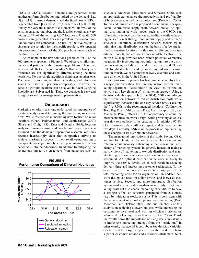
An example of the five solutions generated for 1 of the500 problems appears in Figure 6. We observe similar out-comes and patterns in the remaining problems. Therefore,we conclude that costs and one-day 500-mile delivery per-formance are not significantly different among the threeheuristics. No one single algorithm dominates another one.The genetic algorithm, simulated annealing, and relocationsearch heuristics all perform comparably. However, thegenetic algorithm heuristic can be solved in Excel using theEvolutionary Solver add-in. Thus, we consider it easy andstraightforward for management implementation.

DiscussionMarketing scholars have long understood the importance oflocation analysis in determining the marketing success offirms. While researchers in marketing have focused on retaillocations (Chan, Padmanabhan, and Seetharaman 2007;Ghosh and Craig 1983; Rust and Donthu 1995), locationanalysis of manufacturing and distribution systems has beenassumed to be the domain of operations research. Yet it hasbecome increasingly clear that companies striving toachieve marketing success in their retail operations mustincorporate strategic supply chain planning—distributionnetworks—into their decisions. In addition to mitigating thedeleterious impact on customers from outcomes such as

stockouts (Anderson, Fitzsimons, and Simester 2006), suchan approach can enhance the productivity and profitabilityof both the retailer and the manufacturer (Rust et al. 2004).To this end, this article has proposed a continuous, uncapac-itated, deterministic supply chain network model. An opti-mal distribution network model, such as the CSCD, cansubstantially reduce distribution expenditure while enhanc-ing service levels through continuous supply and reducedstockouts. Traditional distribution network models try tominimize total distribution cost on the basis of a few prede-fined alternative locations. In this study, different from tra-ditional models, we are not given candidate locations; theentire U.S. map provides near-infinite potential warehouselocations. By incorporating key information into the distri-bution system, including zip codes, fuel price, and TL andLTL freight structures, and by converting mileage to carriertime in transit, we can comprehensively examine and com-pare all cities in the United States.

Our proposed approach has been implemented by GSK,a major pharmaceutical firm, in conjunction with the mar-keting department. GlaxoSmithKline views its distributionnetwork as a key element of its marketing strategy. Using adecision calculus approach (Little 2004), GSK can redesignthe distribution network to reduce distribution costs whilesignificantly increasing the one-day service level. Locatingthe five RDCs in the recommended locations (Collinsville,Tex.; Big Pine, Calif.; Shady Dale, Ga.; Lockport, Ill.; andManheim, Penn.) offers GSK the opportunity to attain themost economical network design, while providing an 86.2%next-day service level to its customers. In addition, 97.8%of all customer orders will be complete and delivered withintwo days. Currently, GSK is in the process of implementingthese changes in its distribution networks.

The managerial implications of this study, beyond GSK,are threefold. First, distribution networks play an importantrole in simultaneously enhancing effectiveness and effi-ciency of marketing systems in general. Instead of taking anarrow view of marketing to exclude distribution and man-ufacturing, a more integrative and comprehensive view iswarranted. An optimal distribution network is likely toimprove the service levels, which will result in reducingdelivery time and increasing customer satisfaction. To theextent that distribution costs constitute a large part of thetotal marketing costs for an organization, an updated net-work design can result in dollar savings and increased cus-tomer service. Second, and more important, distributionsystems—if correctly designed—can not only offset mar-keting costs but also enable marketing expenditures to havea stronger effect on revenues generated from customers(e.g., by mitigating stockout costs). This is consistent withthe achievement of a dual emphasis with marketing (Rust,Moorman, and Dickson 2002). The dual emphasis of thisstudy is on achieving a lower total cost while increasing thecustomer service level and with an efficiency orientationadvocated by leading researchers (Rust et al. 2004). Third,the results show the importance of using decision calculusto implement marketing strategy from the “inside out.” Inother words, managerial inputs about key decision variablescan be used to design a system from the inside to obtainsuperior customer service and customer satisfaction. Such

FIGURE 6Performance Comparison of Different Heuristics


an approach can be used by market-oriented firms even inthe absence of direct customer inputs.

In terms of limitations, we acknowledge that differentfirms may have different constraints in their network designother than those addressed in our model. In addition,although inventory holding and backlogging costs werebeyond the scope of this article under the assumptions of adeterministic model and a single period, they can be incor-porated into the model for a more precise estimation of thedistribution costs. Variants of this approach can be devel-oped to suit the specific needs of a given firm. However, wehope that such developments will not only lead to additionaltheoretical insights about the importance of distribution net-work design but also spur research in marketing to enable amore thorough investigation of supply chain issues.

AppendixList of Indexes, Parameters, and

Variables in the CSCD Model

Indexesi: Product type, where I is the total number of product types a

company must transport (i = 1, 2, …, I).j: Plant number, where J is the total number of plants existing

in the supply chain (j = 1, 2, …, J).k: RDC (warehouse) number, where K is the maximum num-

ber of RDCs that can be opened, which can be specified bymanagement or set to a very large number by default. Theoptimal number of RDCs obtained will be equal to or lessthan the K value specified (k = 1, 2, …, K).

l: CDC number where L is the total number of CDCs to beallocated in the supply chain problem (l = 1, 2, …, L).

ParametersF(wk): Cost function of opening and operating RDC k. It is

a function of warehouse size.g: Unit transportation cost from plant j to RDC k per

weighted distance. The cost g can be derived fromEquations 10, 12, and 14.

h: Unit transportation cost from RDC k to CDC l perweighted distance. The cost h can be derived fromEquations 10, 11, and 13.

(aj, bj): Location coordinates of plant j.(al′, bl′): Location coordinates of CDC l.

Dil: Demand for product i by CDC l.

Variables(xk, yk): coordinates of RDC k.

dj(xk, yk): Distance from plant j to RDC k. dj(xk, yk) =

dl(xk, yk): Distance from RDC k to CDC l. dl(xk, yk) =

ukl: Binary variable that takes the value of 1 if RDC kserves CDC l.

zk: Binary variable that takes the value of 1 if RDC kis opened.

sijk: Amount of product i shipped from plant j to RDCk.

tikl: Amount of product i shipped from RDC k to CDCl.

wk: Relative size of RDC k.

( ) ( ) .x a y bk k− + −l l′ ′2 2

( ) ( ) .x a y bk j k j− + −2 2

REFERENCESAmiri, Ali (2006), “Designing a Distribution Network in a Supply

Chain System: Formulation and Efficient Solution Procedure,”European Journal of Operational Research, 171 (June),567–76.

Anderberg, Michael R. (1973), Cluster Analysis for Applicationsin Probability and Mathematical Statistics. New York: Acade-mic Press.

Anderson, Eric T., Gavan J. Fitzsimons, and Duncan Simester(2006), “Measuring and Mitigating the Costs of Stockouts,”Management Science, 52 (November), 1751–63.

Arntzen, Bruce C., Gerald G. Brown, Terry P. Harrison, and LindaL. Trafton (1995), “Global Supply Chain Management at Digi-tal Equipment Corporation,” Interfaces, 25 (January–February), 69–93.

Ashlock, Daniel (2005), Evolutionary Computation for Modelingand Optimization. New York: Springer.

Baumol, William J. and Philip Wolfe (1958), “A Warehouse-Location Problem,” Operations Research, 6 (March–April),252–63.

Beamon, Benita M. (1998), “Supply Chain Design and Analysis:Models and Methods,” International Journal of ProductionEconomics, 55 (August), 281–94.

Brandeau, Margaret L. and Samuel S. Chiu (1989), “An Overviewof Representative Problems in Location Research,” Manage-ment Science, 35 (June), 645–74.

Brimberg, Jack, Pierre Hansen, Nenad Mladenovic, and Eric D.Taillard (2000), “Improvements and Comparison of Heuristicsfor Solving the Uncapacitated Multisource Weber Problem,”Operations Research, 48 (May–June), 444–60.

Brown, Gerald G., Glenn W. Graves, and Maria D. Honczarenko(1987), “Design and Operation of a Multicommodity Produc-tion/Distribution System Using Primal Goal Decomposition,”Management Science, 33 (November), 1469–80.

Bucklin, Louis P. (1967), “The Concept of Mass in Intra-UrbanShopping,” Journal of Marketing, 31 (October), 37–42.

Chakravarti, Dipankar, Andrew Mitchell, and Richard Staelin(1979), “Judgment Based Marketing Decision Models: AnExperimental Investigation of the Decision CalculusApproach,” Management Science, 25 (March), 251–63.

Chan, Tat Y., V. Padmanabhan, and P.B. Seetharaman (2007), “AnEconometric Model of Location and Pricing in the GasolineMarket,” Journal of Marketing Research, 44 (November),622–35.

Cohen, Morris A. and Hau L. Lee (1988), “Strategic Analysis ofIntegrated Production-Distribution Systems: Models and Meth-ods,” Operations Research, 36 (March–April), 216–28.

Cooper, Leon (1964), “Heuristic Methods for Location-AllocationProblems,” SIAM Review, 6 (January), 37–53.

——— (1967), “Solutions of Generalized Locational EquilibriumModels,” Journal of Regional Science, 7 (June), 1–19.

Cox, Reavis (1959), “Consumer Convenience and the Retail Struc-ture of Cities,” Journal of Marketing, 23 (April), 355–62.

Daskin, Mark S. (1995), Network and Discrete Location: Models,Algorithms and Applications. New York: John Wiley & Sons.

Davis, Peter (2006), “Spatial Competition in Retail Markets:Movie Theaters,” Rand Journal of Economics, 37 (December),964–82.


Deveci-Kocakoc, Ipek and Ali Sen (2006), “Utilising Surveys forFinding Improvement Areas for Customer Satisfaction Alongthe Supply Chain,” International Journal of Market Research,48 (5), 623–36.

Devlin, James F. and Philip Gerrard (2004), “Choice Criteria inRetail Banking: An Analysis of Trends,” Journal of StrategicMarketing, 12 (March), 13–27.

Donthu, Naveen and Roland T. Rust (1989), “Estimating Geo-graphic Customer Densities Using Kernel Density Estimation,”Marketing Science, 8 (Spring), 191–203.

Du Merle, Olivier, Daniel Villeneuve, Jacques Desrosiers, andPierre Hansen (1999), “Stabilized Column Generation,” Dis-crete Mathematics, 194 (January), 229–37.

Eiben, Agostan E. and Jim E. Smith (2007), Introduction to Evolu-tionary Computing. New York: Springer.

Elhedhli, Samir and Jean-Louis Goffin (2005), “EfficientProduction-Distribution System Design,” ManagementScience, 51 (July), 1151–64.

Erenguc, Selcuk S., Natalie C. Simpson, and Asoo J. Vakharia(1999), “Integrated Production/Distribution Planning in SupplyChains: An Invited Review,” European Journal of OperationalResearch, 115 (June), 219–36.

Erlenkotter, Donald (1978), “A Dual-Based Procedure for Unca-pacitated Facility Location,” Operations Research, 26(November–December), 992–1009.

Eskigun, Erdem, Reha Uzsoy, Paul V. Preckel, George Beaujon,Subramanian Krishnan, and Jeffrey D. Tew (2005), “OutboundSupply Chain Network Design with Mode Selection, LeadTimes and Capacitated Vehicle Distribution Centers,” Euro-pean Journal of Operational Research, 165 (August), 182–206.

Frontline Systems (2007), Premium Solver. Incline Village, NV:Frontline Systems.

Geoffrion, Arthur M. and Glenn W. Graves (1974), “Multicom-modity Distribution System Design by Benders Decomposi-tion,” Management Science, 20 (January), 822–44.

——— and Richard F. Powers (1995), “20 Years of Strategic Dis-tribution System Design: An Evolutionary Perspective,” Inter-faces, 25 (September–October), 105–127.

Ghosh, Avijit and C. Samuel Craig (1983), “Formulating RetailLocation Strategy in a Changing Environment,” Journal ofMarketing, 47 (Summer), 56–68.

——— and ——— (1986), “An Approach to Determining Opti-mal Locations for New Services,” Journal of MarketingResearch, 23 (November), 354–62.

——— and Sara L. McLafferty (1982), “Locating Stores inUncertain Environments: A Scenario Planning Approach,”Journal of Retailing, 58 (Winter), 5–22.

Gower, John C. (1985), “Measures of Similarity, Dissimilarity andDistance” in Encyclopedia of Statistical Sciences, S. Kotz,Normal L. Johnson, and Campbell B. Read, eds. New York:John Wiley & Sons, 397–405.

Holland, John H. (1975), Adaptation in Natural and Artificial Sys-tems. Ann Arbor: University of Michigan Press.

Iyer, Ananth V. and Mark E. Bergen (1997), “Quick Response inManufacturer-Retailer Channels,” Management Science, 43(April), 559–70.

Jayaraman, Vaidyanathan and Arthur Ross (2003), “A SimulatedAnnealing Methodology to Distribution Network Design andManagement,” European Journal of Operational Research, 144(February), 629–45.

Kadiyali, Vrinda, Pradeep Chintagunta, and Naufel Vilcassim(2000), “Manufacturer-Retailer Channel Interactions andImplications for Channel Power: An Empirical Investigation ofPricing in a Local Market,” Marketing Science, 19 (Spring),127–48.

Klamroth, Kathrin (2001), “Planar Weber Location Problems withLine Barriers,” Optimization, 49 (5–6), 517–27.

Klose, Andreas and Andreas Drexl (2005), “Facility LocationModels for Distribution System Design,” European Journal ofOperational Research, 162 (April), 4–29.

Korpela, Jukka and Antti Lehmusvaara (1999), “A Customer Ori-ented Approach to Warehouse Network Evaluation andDesign,” International Journal of Production Economics, 59(March), 135–46.

Kuo, Ren J., Sheng-Chai Chi, and Shan-Shin Kao (2002), “ADecision Support System for Selecting Convenience StoreLocation Through Integration of Fuzzy AHP and ArtificialNeural Network,” Computers in Industry, 47 (February),199–214.

Langston, Paul, Graham P. Clarke, and Dave B. Clarke (1997),“Retail Saturation, Retail Location, and Retail Competition: AnAnalysis of British Grocery Retailing,” Environment and Plan-ning: A, 29 (January), 77–104.

Little, John D.C. (2004), “Comments on ‘Models and Managers:The Concept of a Decision Calculus,’” Management Science,50 (December), 1854–60.

Lord, Dennis J. and Charles Lynds (1981), “The Use of Regres-sion Models in Store Location Research: A Review and CaseStudy,” Akron Business and Economic Review, 12 (Summer),13–19.

Mahajan,Vijay, Subhash Sharma, and Roger A. Kerin (1988),“Assessing Market Opportunities and Saturation Potential forMulti-Store, Multi-Market Retailers,” Journal of Retailing, 64(Fall), 315–32.

Meepetchdee, Yongyut and Nilay Shah (2007), “Logistical Net-work Design with Robustness and Complexity Considera-tions,” International Journal of Physical Distribution & Logis-tical Management, 37 (March), 202–222.

Melkote, Sanjay and Mark S. Daskin (2001), “Capacitated FacilityLocation/Network Design Problems,” European Journal ofOperational Research, 129 (March), 481–95.

Menon, Anil (2004), Frontiers of Evolutionary Computation(Genetic Algorithms and Evolutionary Computation). NewYork: Springer Publishing Company.

Mittal, Vikas, Wagner A. Kamakura, and Rahul Govind (2004),“Geographic Patterns in Customer Service and Satisfaction: AnEmpirical Investigation,” Journal of Marketing, 68 (July),48–62.

Moon, Douglas I. and Sohail S. Chaudhry (1984), “An Analysis ofNetwork Location Problems with Distance Constraints,” Man-agement Science, 30 (March), 290–307.

Mulhern, Francis J. (1997), “Retail Marketing: From Distributionto Integration,” International Journal of Research in Market-ing, 14 (May), 103–124.

Murry, John P., Jr., and Jan B. Heide (1998), “Managing Promo-tion Program Participation Within Manufacturer–Retailer Rela-tionships,” Journal of Marketing, 62 (January), 58–68.

Pinkse, Joris, Margaret E. Slade, and Craig Brett (2002), “SpatialPrice Competition: A Semiparametric Approach,” Economet-rica, 70 (May), 1111–53.

Rosing, Kenneth E. (1992), “An Optimal Method for Solving the(Generalized) Multi-Weber Problem,” European Journal ofOperational Research, 58 (May), 414–26.

Rust, Roland T., Tim Ambler, Gregory S. Carpenter, V. Kumar,and Rajendra K. Srivastava (2004), “Measuring Marketing Pro-ductivity: Current Knowledge and Future Directions,” Journalof Marketing, 68 (October), 76–89.

——— and Naveen Donthu (1995), “Capturing GeographicallyLocalized Misspecification Error in Retail Store Choice Mod-els,” Journal of Marketing Research, 32 (February), 103–110.

———, Christine Moorman, and Peter R. Dickson (2002), “Get-ting Return on Quality: Revenue Expansion, Cost Reduction,or Both?” Journal of Marketing, 66 (October), 7–24.

Saourirajan, Karthik, Leyla Ozsen, and Reha Uzsoy (2007), “ASingle-Product Network Design Model with Lead Time and


Safety Stock Considerations,” IIE Transactions, 39 (May),411–24.

Shen, Zuo-Jun M. (2005), “A Multi-Commodity Supply ChainDesign Problem,” IIE Transactions, 37 (August), 753–62.

Swersey, Arthur and Lakshman S. Thakur (1995), “An Integer Pro-gramming Model for Locating Vehicle Emission Testing Sta-tions,” Management Science, 41 (March), 496–512.

Thelen, Eva M. and Arch G. Woodside (1997), “What Evokes theBrand or Store? Consumer Research on Accessibility TheoryApplied to Modeling Primary Choice,” International Journalof Research in Marketing, 14 (May), 125–45.

Vidal, Carlos J. and Marc Goetschalckx (1997), “StrategicProduction-Distribution Models: A Critical Review withEmphasizes on Global Supply Chain Models,” European Jour-nal of Operational Research, 98 (April), 1–18.

Wen, Meilin and Kakuzo Iwamura (2008), “Fuzzy FacilityLocation-Allocation Problem Under the Hurwicz Criterion,”European Journal of Operational Research, 184 (January),627–35.

Wesolowsky, George O. (1993), “The Weber Problem: History andPerspectives,” Location Science, 1 (January), 5–23.

Documents

Distribution Network Redesign for Marketing … Shang, Tuba Pinar Yildirim, Pandu Tadikamalla, Vikas Mittal, & Lawrence H. Brown Distribution Network Redesign for Marketing Competitiveness