Embed Size (px)
Citation preview
Distributed System Design:
An Overview*
Jie Wu
Department of Computer and
Information Sciences
Temple University
Philadelphia, PA 19122
*Part of the materials come from Distributed System Design, CRC Press, 1999.
(Chinese Edition, China Machine Press, 2001.)
The Structure of Classnotes
Focus
Example
Exercise
Project

Table of Contents
Introduction and Motivation
Theoretical Foundations
Distributed Programming Languages
Distributed Operating Systems
Distributed Communication
Distributed Data Management
Reliability
Applications
Conclusions
Appendix
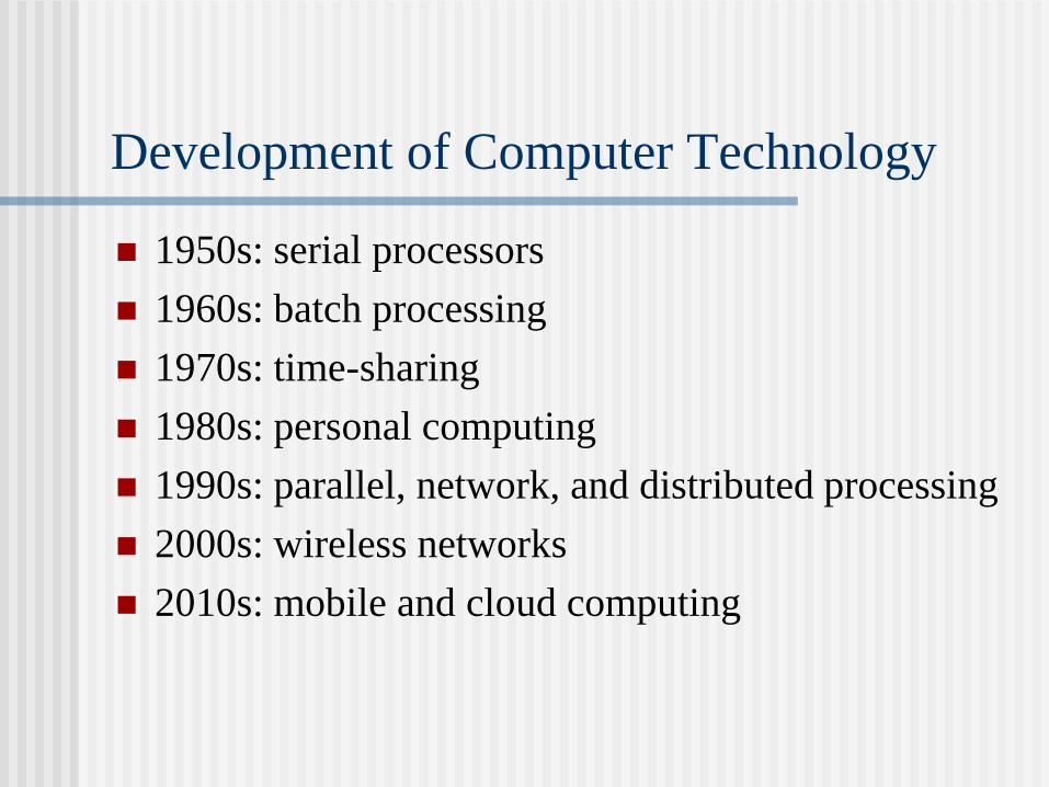
Development of Computer Technology
1950s: serial processors
1960s: batch processing
1970s: time-sharing
1980s: personal computing
1990s: parallel, network, and distributed processing
2000s: wireless networks
2010s: mobile and cloud computing
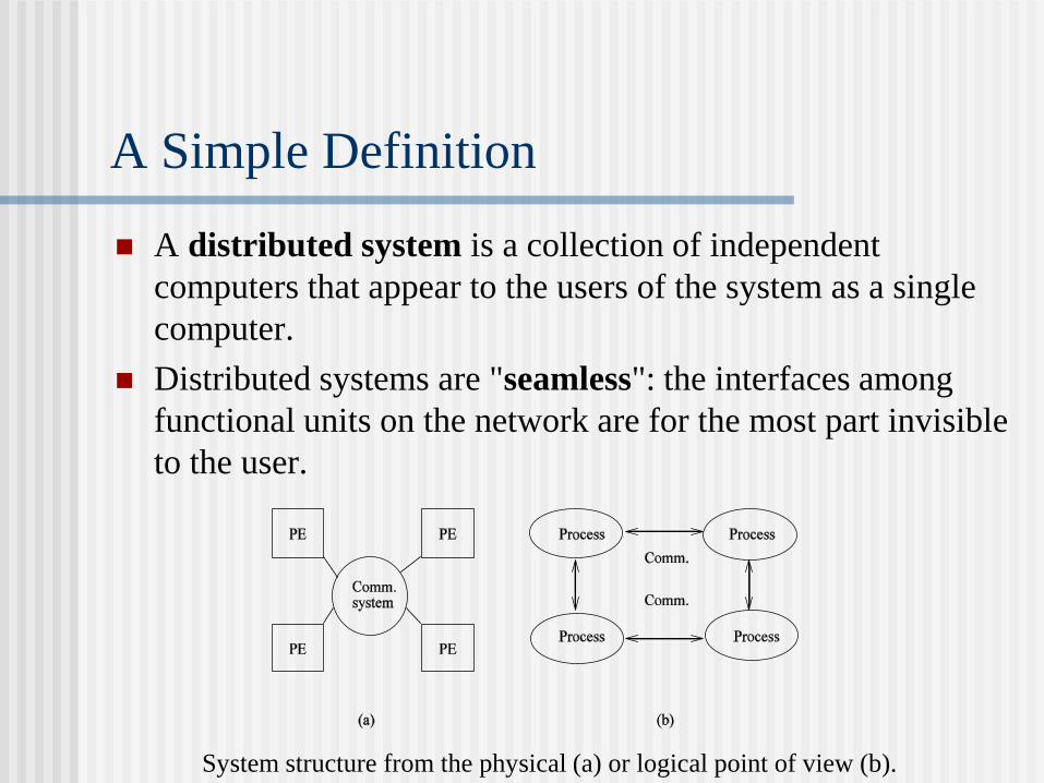
A distributed system is a collection of independent
computers that appear to the users of the system as a single
computer.
Distributed systems are "seamless": the interfaces among
functional units on the network are for the most part invisible
to the user.
System structure from the physical (a) or logical point of view (b).
A Simple Definition
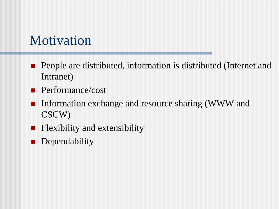
Motivation
People are distributed, information is distributed (Internet and
Intranet)
Performance/cost
Information exchange and resource sharing (WWW and
CSCW)
Flexibility and extensibility
Dependability
Two Main Stimuli
Technological change
User needs
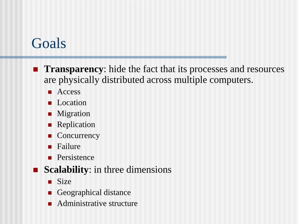
Goals
Transparency: hide the fact that its processes and resources are physically distributed across multiple computers.
Access
Location
Migration
Replication
Concurrency
Failure
Persistence
Scalability: in three dimensions
Size
Geographical distance
Administrative structure

Goals (Cont’d.)
Heterogeneity (mobile code and mobile agent)
Networks
Hardware
Operating systems and middleware
Program languages
Openness
Security
Fault Tolerance
Concurrency
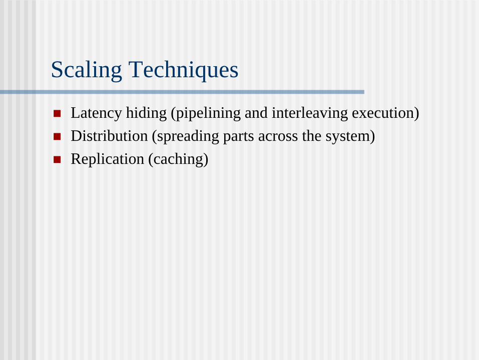
Scaling Techniques
Latency hiding (pipelining and interleaving execution)
Distribution (spreading parts across the system)
Replication (caching)

Example 1: (Scaling Through Distribution)
URL searching based on hierarchical DNS name space (partitioned into zones).
DNS name space.
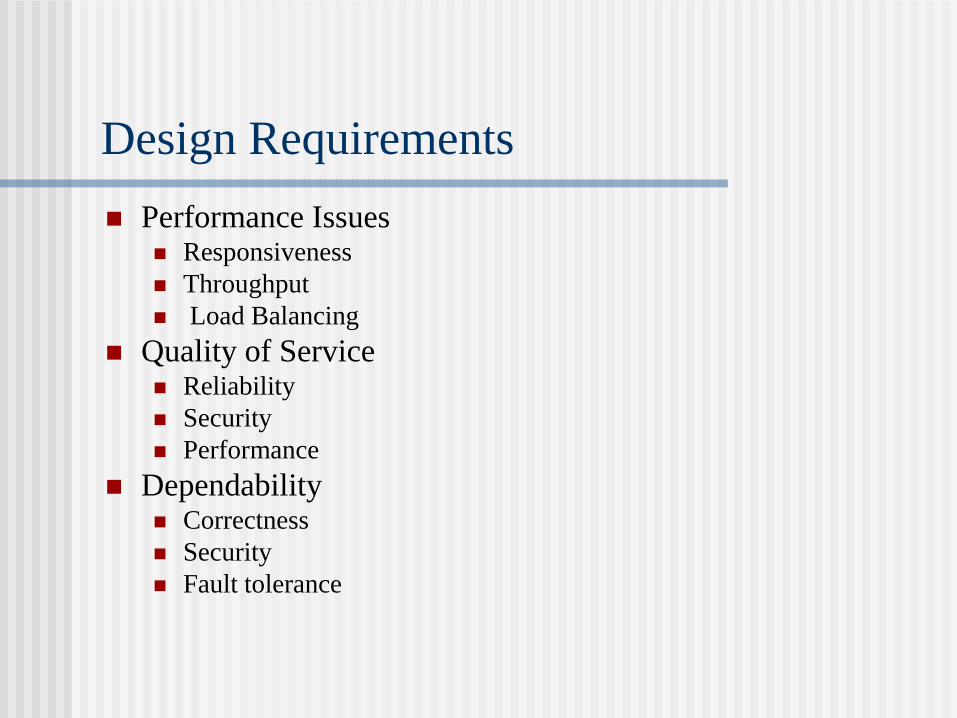
Design Requirements
Performance Issues Responsiveness
Throughput
Load Balancing
Quality of Service Reliability
Security
Performance
Dependability Correctness
Security
Fault tolerance
Similar and Related Concepts
Distributed
Network
Parallel
Concurrent
Decentralized
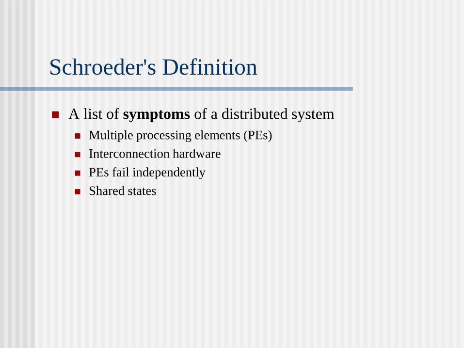
Schroeder's Definition
A list of symptoms of a distributed system Multiple processing elements (PEs)
Interconnection hardware
PEs fail independently
Shared states
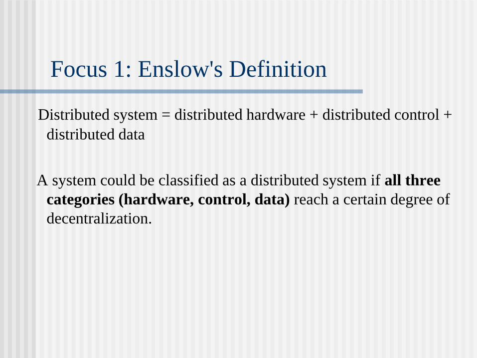
Focus 1: Enslow's Definition
Distributed system = distributed hardware + distributed control +
distributed data
A system could be classified as a distributed system if all three
categories (hardware, control, data) reach a certain degree of
decentralization.

Focus 1 (Cont’d.)
Enslow's model of distributed systems.
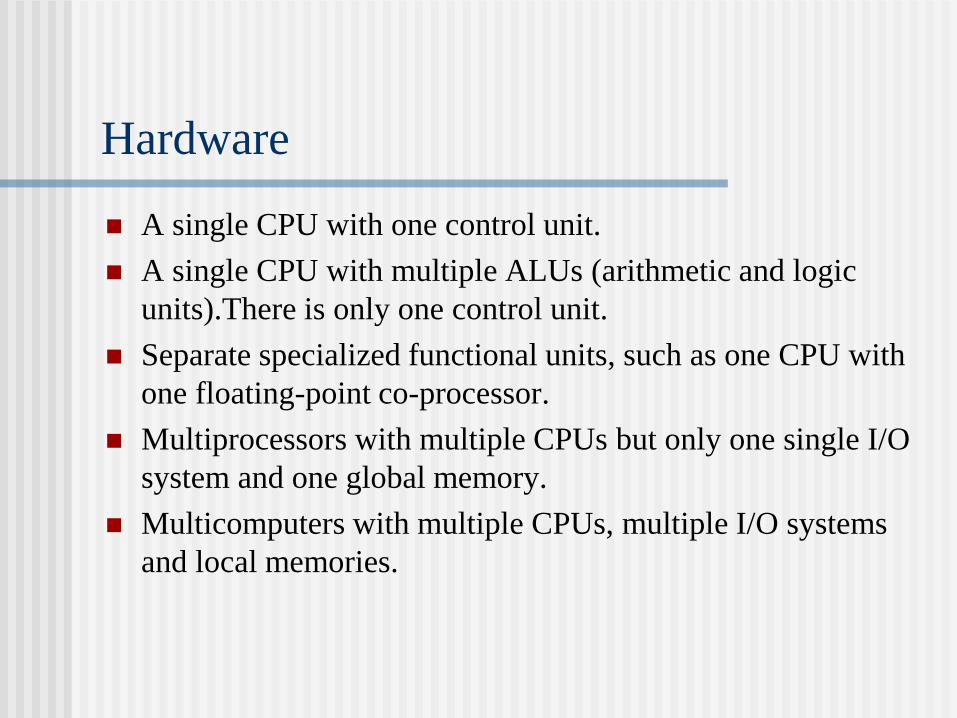
Hardware
A single CPU with one control unit.
A single CPU with multiple ALUs (arithmetic and logic
units).There is only one control unit.
Separate specialized functional units, such as one CPU with
one floating-point co-processor.
Multiprocessors with multiple CPUs but only one single I/O
system and one global memory.
Multicomputers with multiple CPUs, multiple I/O systems
and local memories.
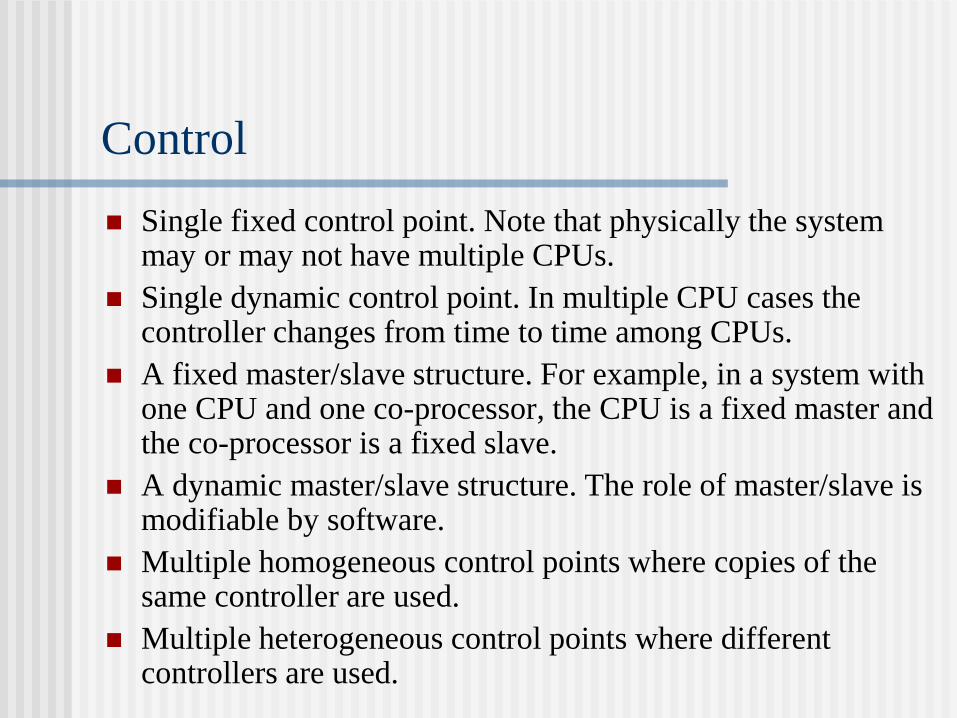
Control
Single fixed control point. Note that physically the system may or may not have multiple CPUs.
Single dynamic control point. In multiple CPU cases the controller changes from time to time among CPUs.
A fixed master/slave structure. For example, in a system with one CPU and one co-processor, the CPU is a fixed master and the co-processor is a fixed slave.
A dynamic master/slave structure. The role of master/slave is modifiable by software.
Multiple homogeneous control points where copies of the same controller are used.
Multiple heterogeneous control points where different controllers are used.
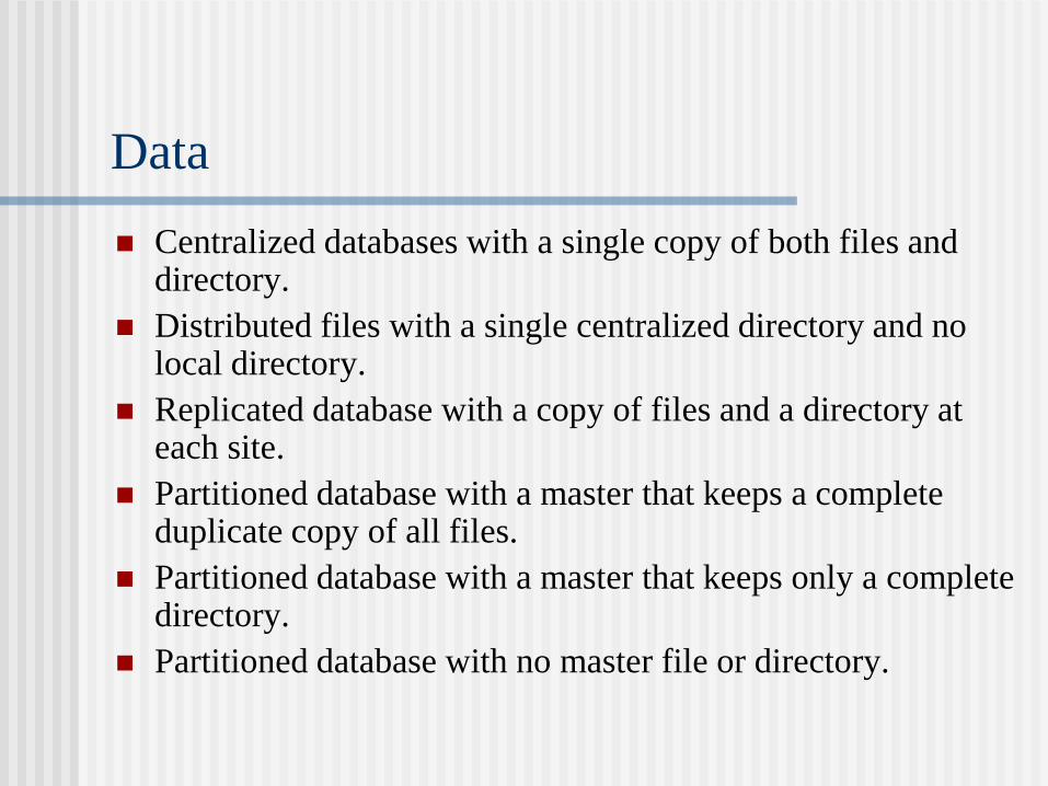
Data
Centralized databases with a single copy of both files and directory.
Distributed files with a single centralized directory and no local directory.
Replicated database with a copy of files and a directory at each site.
Partitioned database with a master that keeps a complete duplicate copy of all files.
Partitioned database with a master that keeps only a complete directory.
Partitioned database with no master file or directory.

Network Systems
Performance scales on throughput (transaction response time
or number of transactions per second) versus load.
Work on burst mode.
Suitable for small transaction-oriented programs (collections
of small, quick, distributed applets).
Handle uncoordinated processes.
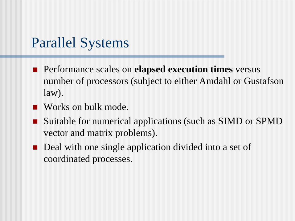
Parallel Systems
Performance scales on elapsed execution times versus
number of processors (subject to either Amdahl or Gustafson
law).
Works on bulk mode.
Suitable for numerical applications (such as SIMD or SPMD
vector and matrix problems).
Deal with one single application divided into a set of
coordinated processes.
Distributed Systems
A compromise of network and parallel
systems.

Comparison
Comparison of three different systems.
Item Network sys. Distributed sys. Multiprocessors
Like a virtual
uniprocessor
No Yes Yes
Run the same operating
system
No Yes Yes
Copies of the operating
system
N copies N copies 1 copy
Means of
communication
Shared files Messages Shared files
Agreed up network
protocols?
Yes Yes No
A single run queue No Yes Yes
Well defined file
sharing
Usually no Yes Yes
Focus 2: Different Viewpoints
Architecture viewpoint
Interconnection network viewpoint
Memory viewpoint
Software viewpoint
System viewpoint
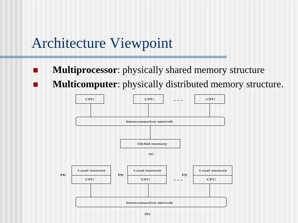
Architecture Viewpoint
Multiprocessor: physically shared memory structure
Multicomputer: physically distributed memory structure.
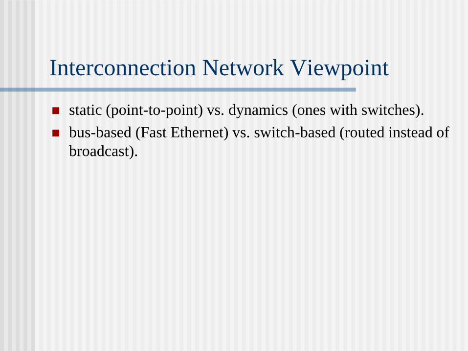
Interconnection Network Viewpoint
static (point-to-point) vs. dynamics (ones with switches).
bus-based (Fast Ethernet) vs. switch-based (routed instead of
broadcast).
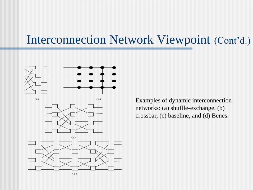
Interconnection Network Viewpoint (Cont’d.)
Examples of dynamic interconnection
networks: (a) shuffle-exchange, (b)
crossbar, (c) baseline, and (d) Benes.
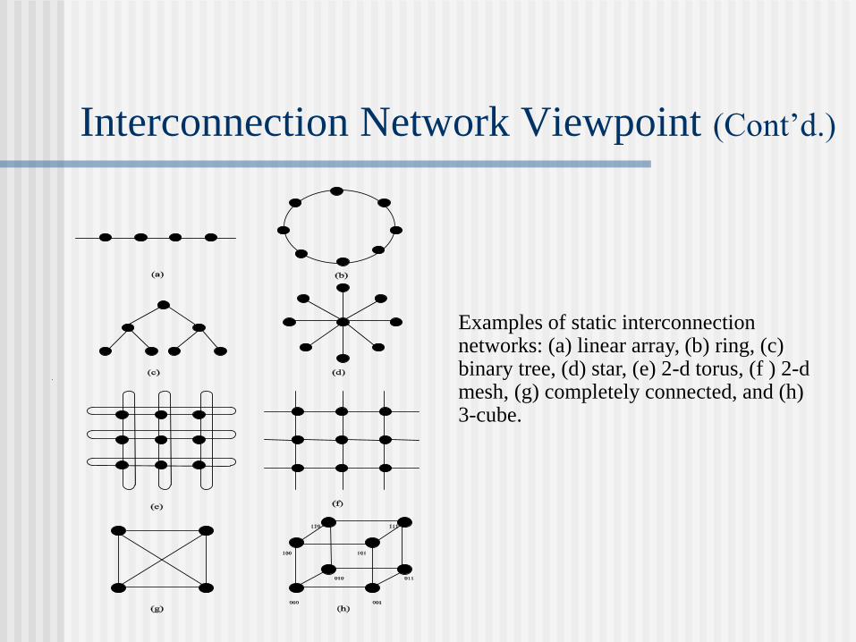
Interconnection Network Viewpoint (Cont’d.)
Examples of static interconnection networks: (a) linear array, (b) ring, (c) binary tree, (d) star, (e) 2-d torus, (f ) 2-d mesh, (g) completely connected, and (h) 3-cube.
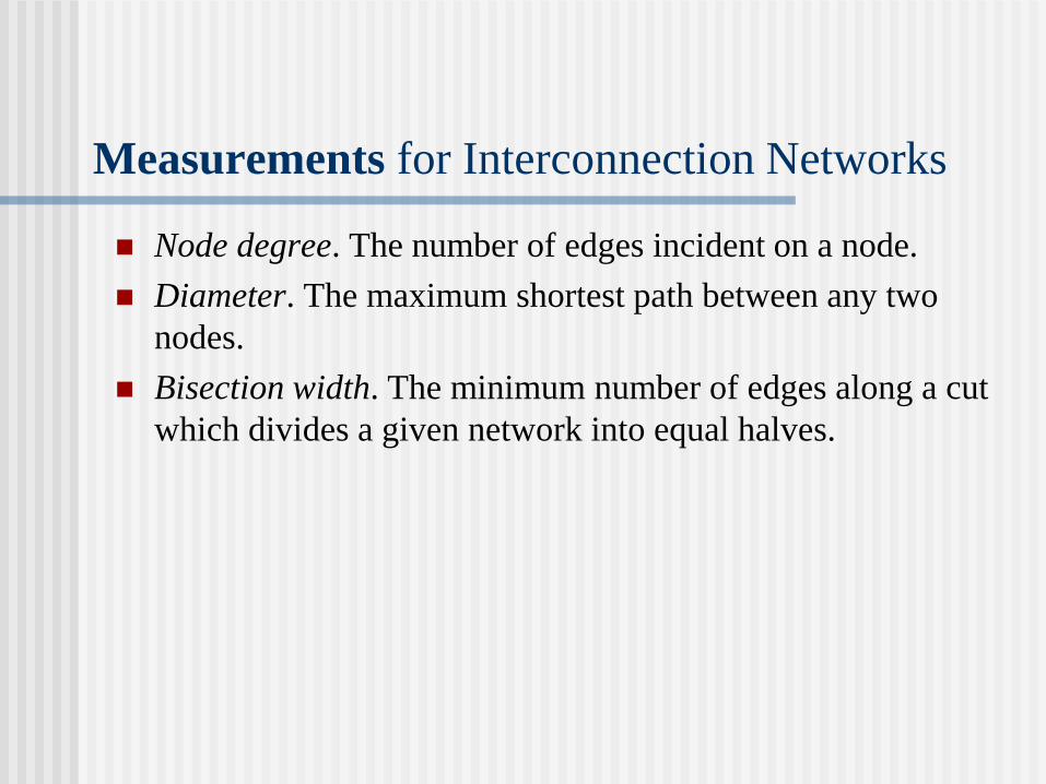
Measurements for Interconnection Networks
Node degree. The number of edges incident on a node.
Diameter. The maximum shortest path between any two
nodes.
Bisection width. The minimum number of edges along a cut
which divides a given network into equal halves.
What's the Best Choice? (Siegel 1994)
A compiler-writer prefers a network where the transfer time
from any source to any destination is the same to simplify the
data distribution.
A fault-tolerant researcher does not care about the type of
network as long as there are three copies for redundancy.
A European researcher prefers a network with a node
degree no more than four to connect Transputers.
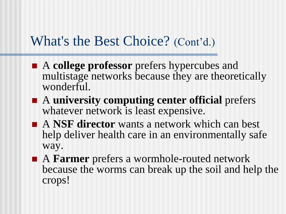
What's the Best Choice? (Cont’d.)
A college professor prefers hypercubes and multistage networks because they are theoretically wonderful.
A university computing center official prefers whatever network is least expensive.
A NSF director wants a network which can best help deliver health care in an environmentally safe way.
A Farmer prefers a wormhole-routed network because the worms can break up the soil and help the crops!
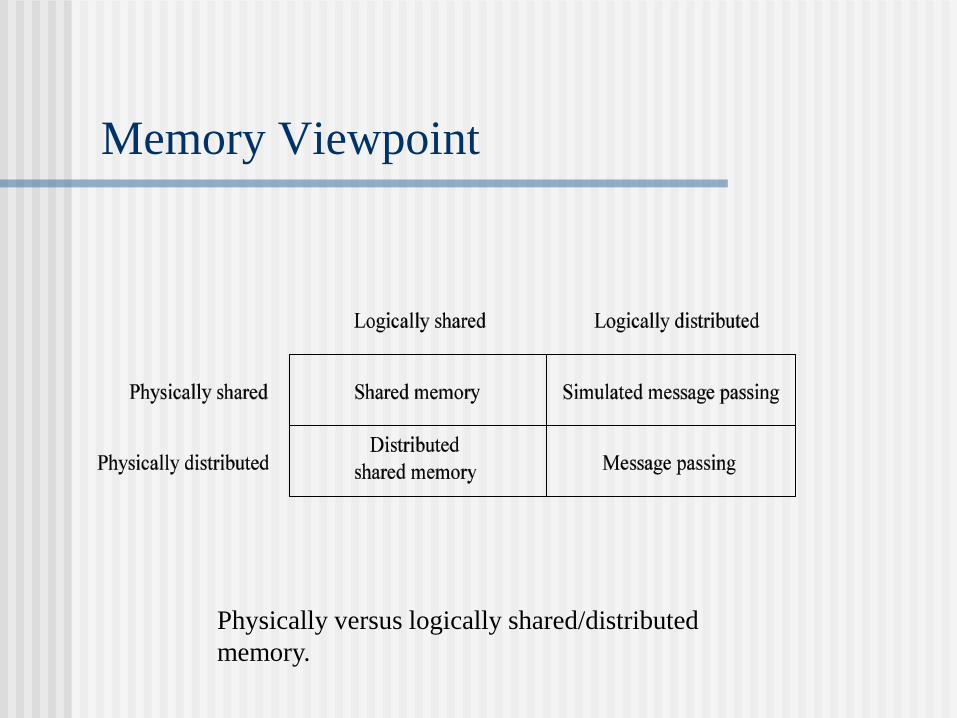
Memory Viewpoint
Physically versus logically shared/distributed
memory.
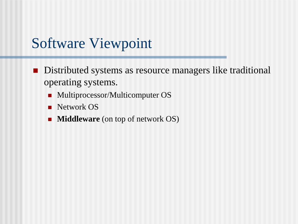
Software Viewpoint
Distributed systems as resource managers like traditional
operating systems.
Multiprocessor/Multicomputer OS
Network OS
Middleware (on top of network OS)
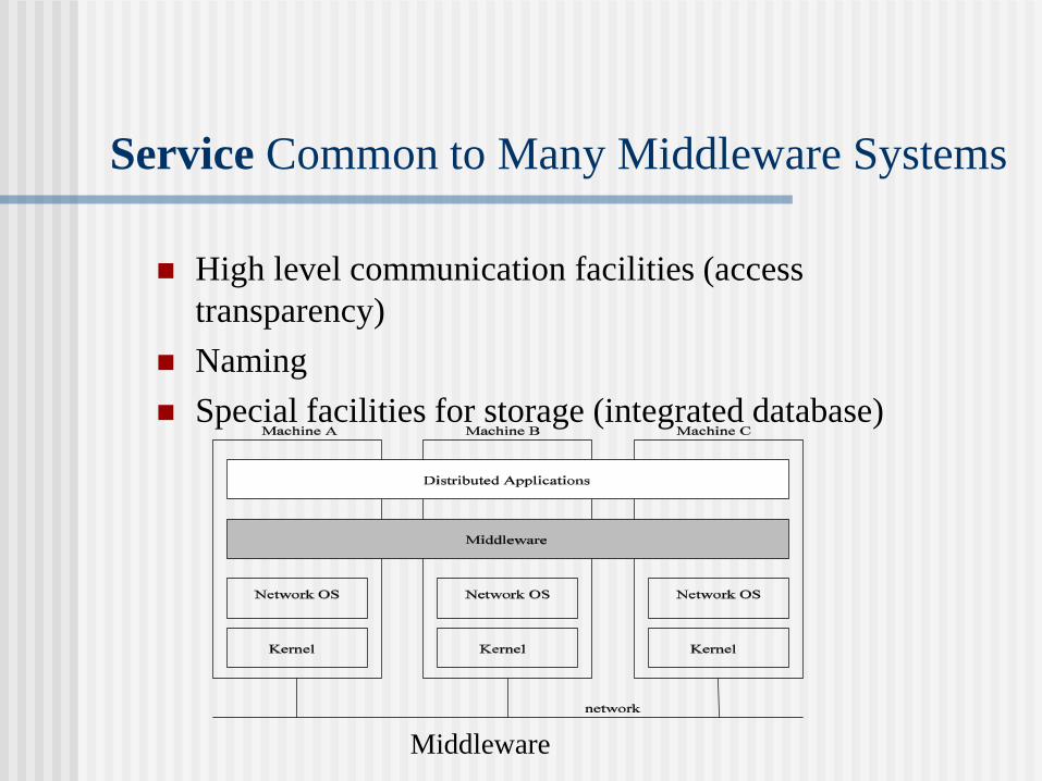
Service Common to Many Middleware Systems
High level communication facilities (access
transparency)
Naming
Special facilities for storage (integrated database)
Middleware

System Viewpoint
The division of responsibilities between system components
and placement of the components.
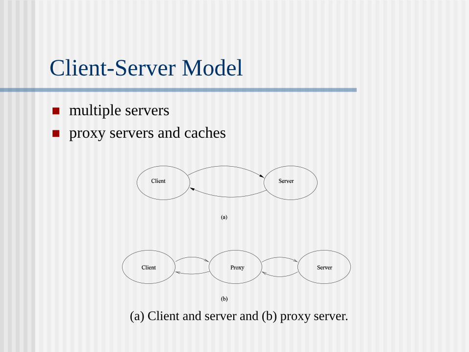
Client-Server Model
multiple servers
proxy servers and caches
(a) Client and server and (b) proxy server.
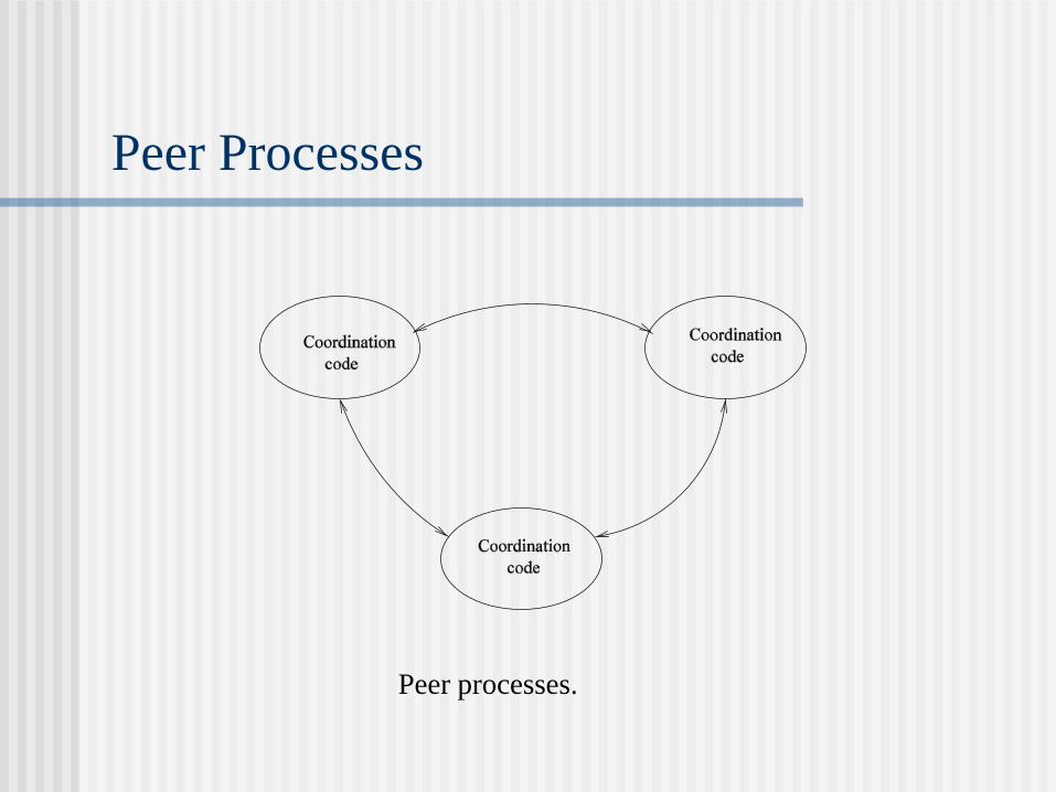
Peer Processes
Peer processes.
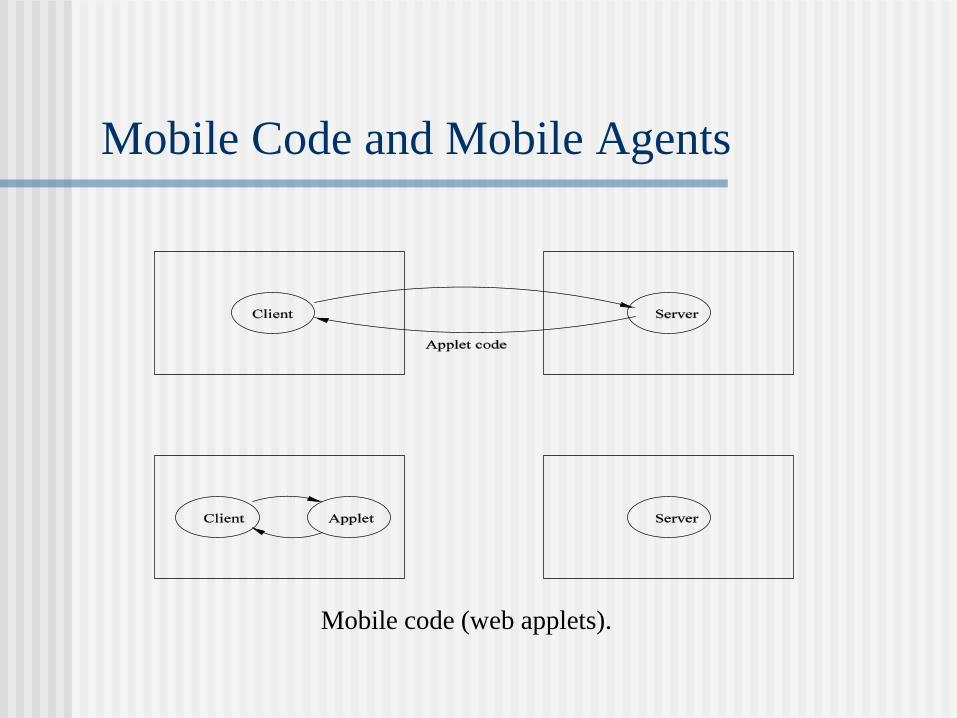
Mobile Code and Mobile Agents
Mobile code (web applets).
Prototype Implementations
Mach (Carnegie Mellon University)
V-kernel (Stanford University)
Sprite (University of California, Berkeley)
Amoeba (Vrije University in Amsterdam)
Systems R (IBM)
Locus (University of California, Los Angeles)
VAX-Cluster (Digital Equipment Corporation)
Spring (University of Massachusetts, Amherst)
I-WAY (Information Wide Area Year): High-performance computing centers interconnected through the Internet.
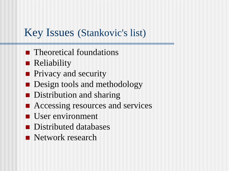
Theoretical foundations
Reliability
Privacy and security
Design tools and methodology
Distribution and sharing
Accessing resources and services
User environment
Distributed databases
Network research
Key Issues (Stankovic's list)
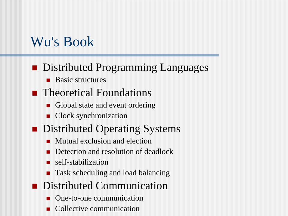
Wu's Book
Distributed Programming Languages Basic structures
Theoretical Foundations Global state and event ordering
Clock synchronization
Distributed Operating Systems Mutual exclusion and election
Detection and resolution of deadlock
self-stabilization
Task scheduling and load balancing
Distributed Communication One-to-one communication
Collective communication

Wu's Book (Cont’d.)
Reliability Agreement
Error recovery
Reliable communication
Distributed Data Management Consistency of duplicated data
Distributed concurrency control
Applications Distributed operating systems
Distributed file systems
Distributed database systems
Distributed shared memory
Distributed heterogeneous systems
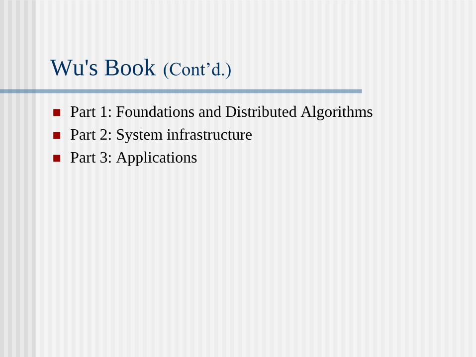
Wu's Book (Cont’d.)
Part 1: Foundations and Distributed Algorithms
Part 2: System infrastructure
Part 3: Applications
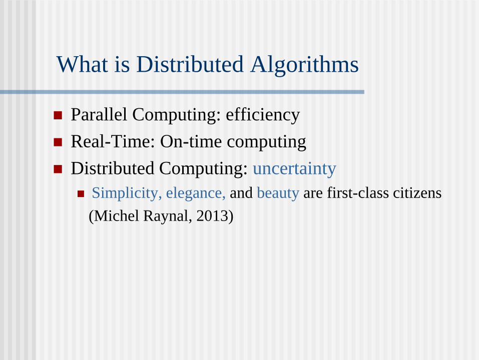
What is Distributed Algorithms
Parallel Computing: efficiency
Real-Time: On-time computing
Distributed Computing: uncertainty
Simplicity, elegance, and beauty are first-class citizens
(Michel Raynal, 2013)
Distributed Message-Passing Algorithms
Termination
In a social network, each person exchanges his/her friend
list with friends. What is the stoppage condition?
Global State
How to design an observation algorithm by observing an
execution without modifying its behavior?
Distributed Consensus
How to reach distributed consensus (e.g., binary
decisions) in the presence of traitors?
Distributed Message-Passing Algorithms
Logical Clock
How to order events in different systems with
asynchronous clocks? How to discard obsolete data?
Data
How to replicate data and keep them consistent?
Load
How to distribute load in a load balanced way?
Routing
How to perform efficient routing that is deadlock-free
and fault-tolerant?
References
IEEE Transactions on Parallel and Distributed Systems (TPDS)
Journal of Parallel and Distributed Computing (JPDC)
Distributed Computing
IEEE International Conference on Distributed Computing Systems (ICDCS)
IEEE International Conference on Reliable Distributed Systems (SRDS)
ACM Symposium on Principles of Distributed Computing (PODC)
IEEE Concurrency (formerly IEEE Parallel & Distributed Technology: Systems & Applications)

Exercise 1
1. In your opinion, what is the future of the computing and
the field of distributed systems?
2. Use your own words to explain the differences between
distributed systems, multiprocessors, and network systems.
3. Calculate (a) node degree, (b) diameter, (c) bisection width,
and (d) the number of links for an n x n 2-d mesh, an n x n 2-
d torus, and an n-dimensional hypercube.
Table of Contents
Introduction and Motivation
Theoretical Foundations
Distributed Programming Languages
Distributed Operating Systems
Distributed Communication
Distributed Data Management
Reliability
Applications
Conclusions
Appendix
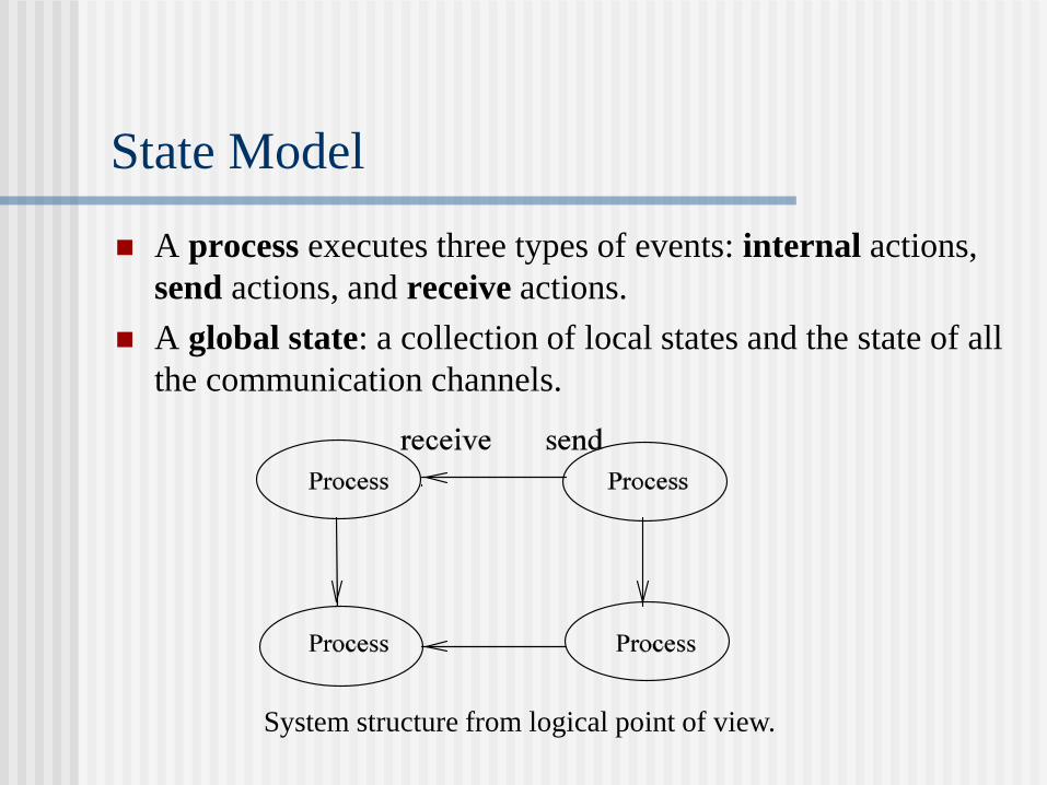
State Model
A process executes three types of events: internal actions,
send actions, and receive actions.
A global state: a collection of local states and the state of all
the communication channels.
System structure from logical point of view.
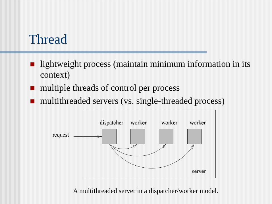
Thread
lightweight process (maintain minimum information in its
context)
multiple threads of control per process
multithreaded servers (vs. single-threaded process)
A multithreaded server in a dispatcher/worker model.
Happened-Before Relation
The happened-before relation (denoted by ) is
defined as follows:
Rule 1 : If a and b are events in the same process and a was
executed before b, then a b.
Rule 2 : If a is the event of sending a message by one process
and b is the event of receiving that message by another
process, then a b.
Rule 3 : If a b and b c, then a c.
Relationship Between Two Events
Two events a and b are causally related if a b or b a.
Two distinct events a and b are said to be concurrent if a
b and b a (denoted as a || b).
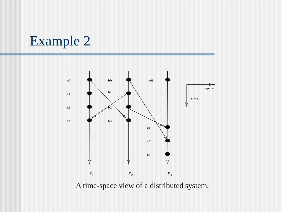
Example 2
A time-space view of a distributed system.

Example 2 (Cont’d.)
Rule 1: a0 a1 a2 a3
b0 b1 b2 b3
c0 c1 c2 c3
Rule 2: a0 b3
b1 a3, b2 c1, b0 c2
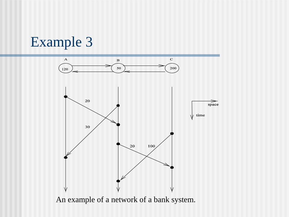
Example 3
An example of a network of a bank system.
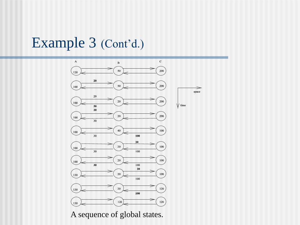
Example 3 (Cont’d.)
A sequence of global states.

Consistent Global State
Four types of cut that cross
a message transmission line.

Consistent Global State (Cont’d.)
A cut is consistent iff no two cut events are causally
related.
Strongly consistent: no (c) and (d).
Consistent: no (d) (orphan message).
Inconsistent: with (d).
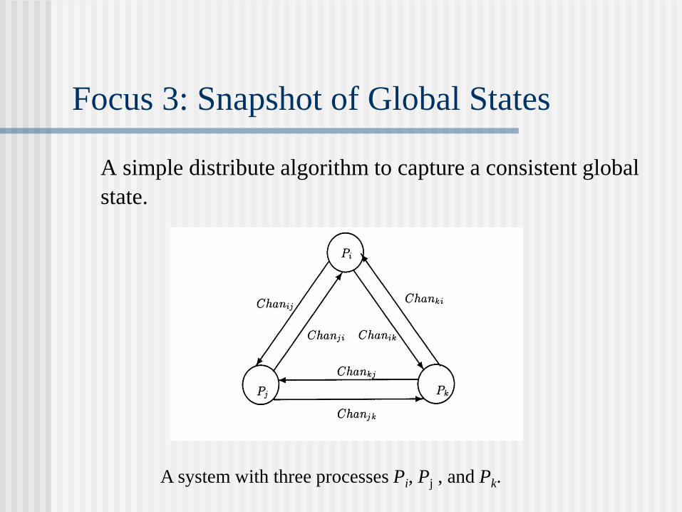
Focus 3: Snapshot of Global States
A simple distribute algorithm to capture a consistent global
state.
A system with three processes Pi, Pj , and Pk.
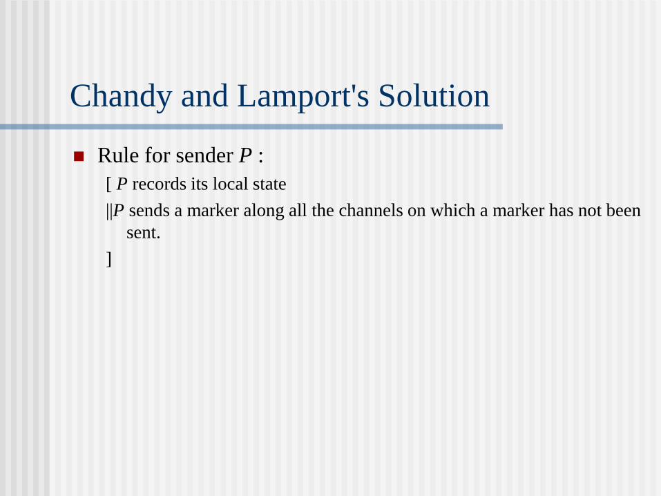
Chandy and Lamport's Solution
Rule for sender P :
[ P records its local state
||P sends a marker along all the channels on which a marker has not been
sent.
]
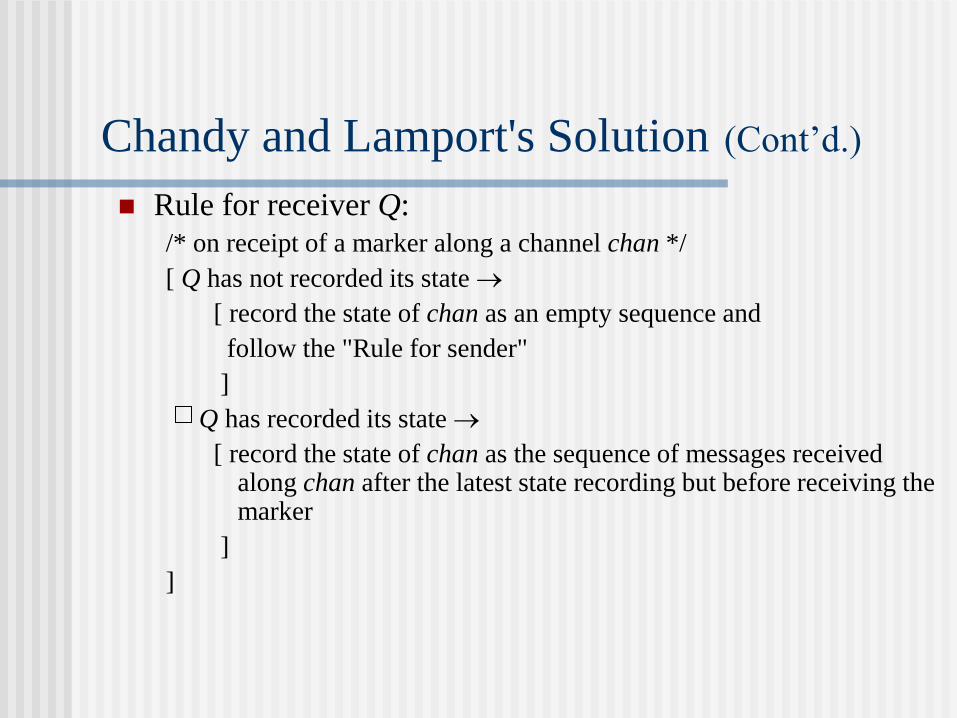
Chandy and Lamport's Solution (Cont’d.)
Rule for receiver Q:
/* on receipt of a marker along a channel chan */
[ Q has not recorded its state
[ record the state of chan as an empty sequence and
follow the "Rule for sender"
]
Q has recorded its state
[ record the state of chan as the sequence of messages received along chan after the latest state recording but before receiving the marker
]
]
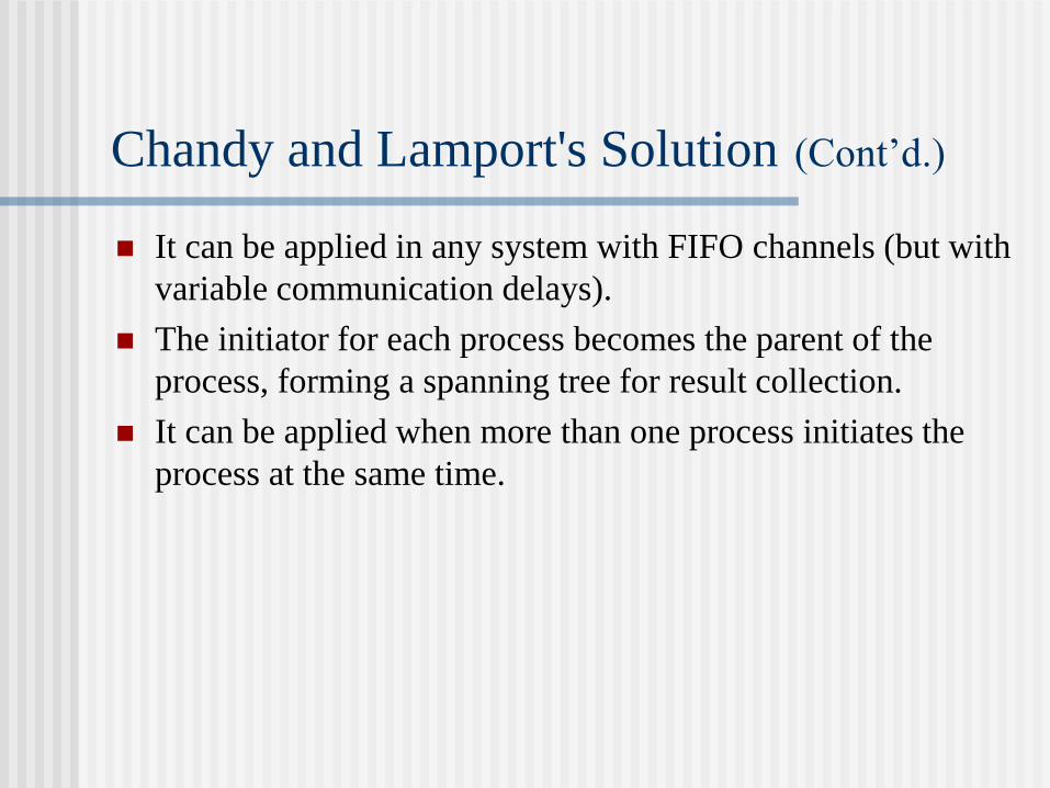
Chandy and Lamport's Solution (Cont’d.)
It can be applied in any system with FIFO channels (but with
variable communication delays).
The initiator for each process becomes the parent of the
process, forming a spanning tree for result collection.
It can be applied when more than one process initiates the
process at the same time.
Focus 4: Lamport's Logical Clocks
Based on a “happen-before” relation that defines a partial order on events
Rule1. Before producing an event (an external send or internal event), we update LC :
LCi = LCi + d (d > 0)
(d can have a different value at each application of Rule1)
Rule2. When it receives the time-stamped message (m, LCj , j), Pi executes the update
LCi = max{Lci, LCj} + d (d > 0)
Focus 4 (Cont’d.)
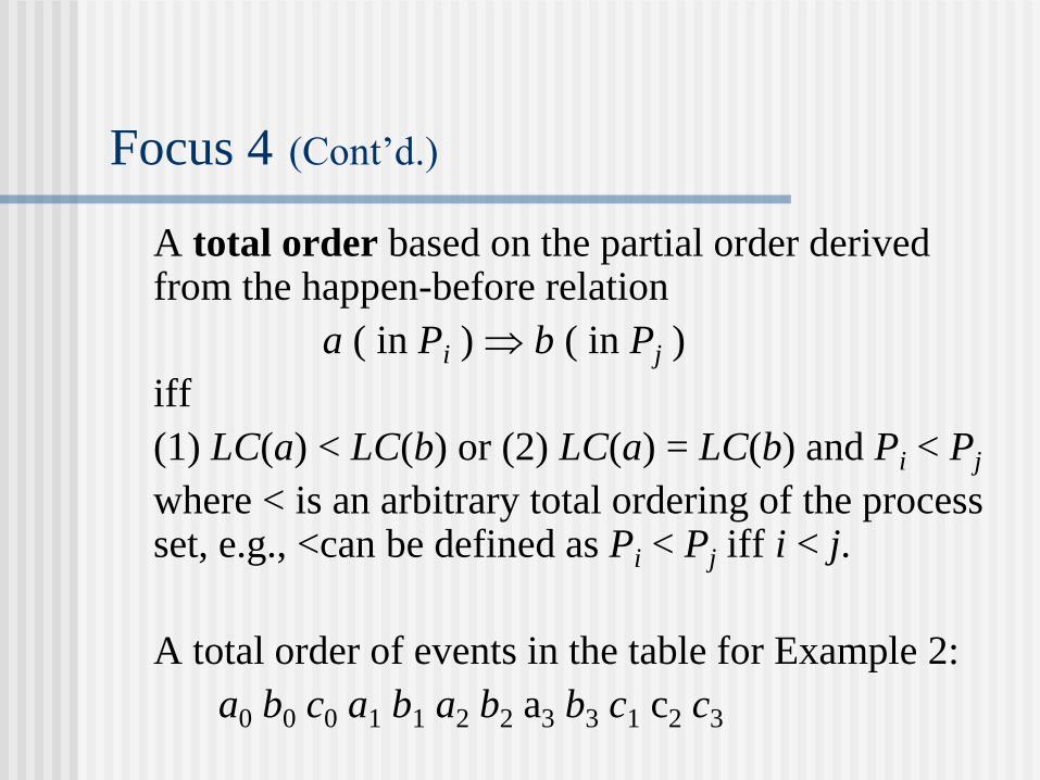
A total order based on the partial order derived from the happen-before relation
a ( in Pi ) b ( in Pj )
iff
(1) LC(a) < LC(b) or (2) LC(a) = LC(b) and Pi < Pj
where < is an arbitrary total ordering of the process set, e.g., <can be defined as Pi < Pj iff i < j.
A total order of events in the table for Example 2:
a0 b0 c0 a1 b1 a2 b2 a3 b3 c1 c2 c3

Example 4: Totally-Ordered Multicasting
Two copies of the account at A and B (with balance of
$10,000).
Update 1: add $1,000 at A.
Update 2: add interests (based on 1% interest rate) at B.
Update 1 followed by Update 2: $11,110.
Update 2 followed by Update 1: $11,100.
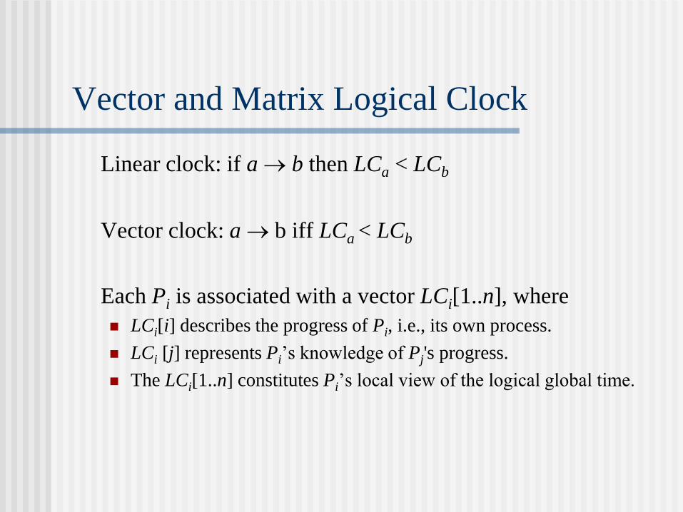
Vector and Matrix Logical Clock
Linear clock: if a b then LCa < LCb
Vector clock: a b iff LCa < LCb
Each Pi is associated with a vector LCi[1..n], where
LCi[i] describes the progress of Pi, i.e., its own process.
LCi [j] represents Pi’s knowledge of Pj's progress.
The LCi[1..n] constitutes Pi’s local view of the logical global time.
Vector and Matrix Logical Clock (Cont’d.)
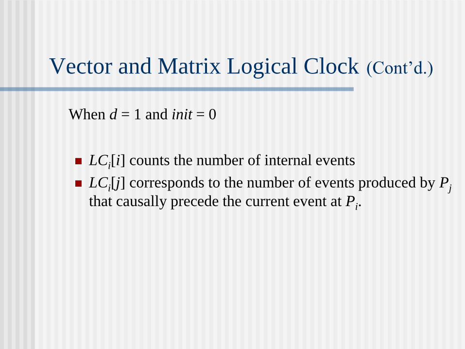
When d = 1 and init = 0
LCi[i] counts the number of internal events
LCi[j] corresponds to the number of events produced by Pj
that causally precede the current event at Pi.
Vector and Matrix Logical Clock (Cont’d.)
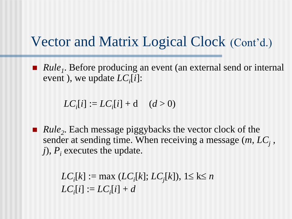
Rule1. Before producing an event (an external send or internal event ), we update LCi[i]:
LCi[i] := LCi[i] + d (d > 0)
Rule2. Each message piggybacks the vector clock of the sender at sending time. When receiving a message (m, LCj , j), Pi executes the update.
LCi[k] := max (LCi[k]; LCj[k]), 1 k n
LCi[i] := LCi[i] + d
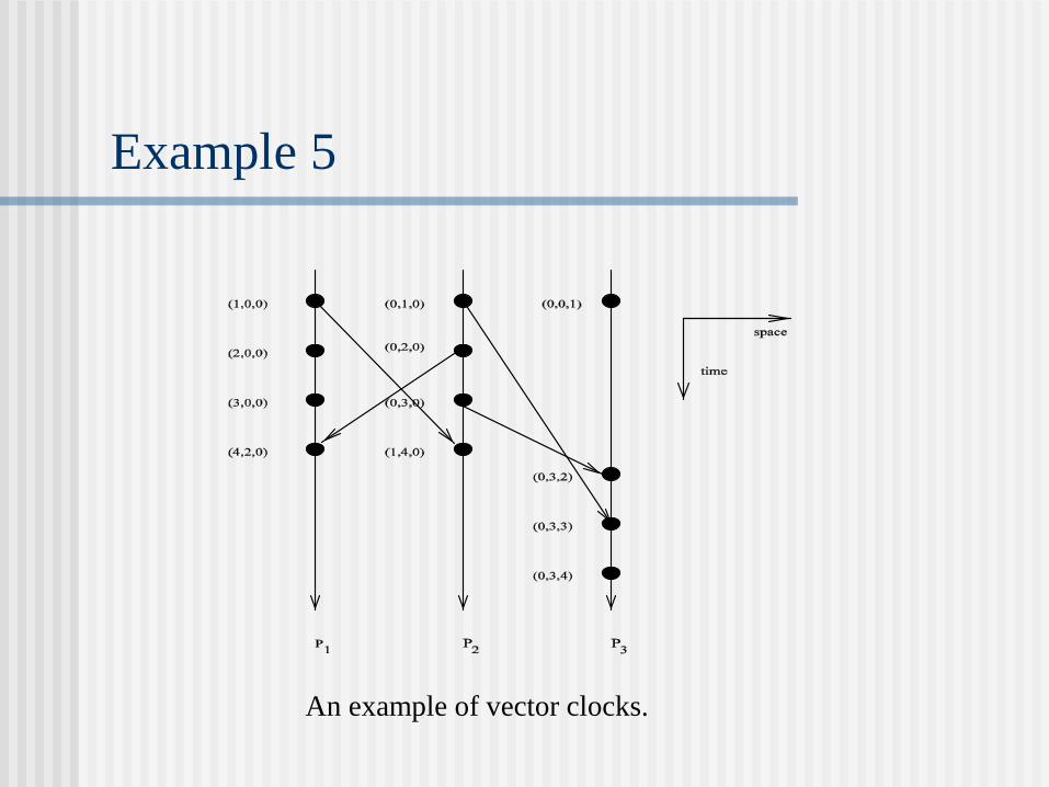
Example 5
An example of vector clocks.
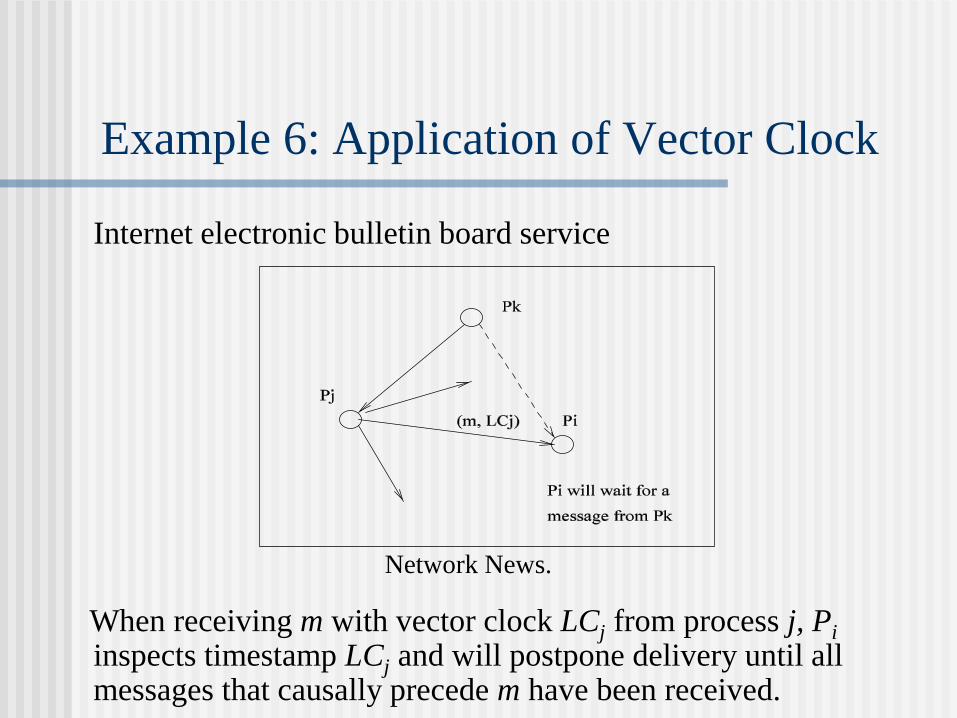
Example 6: Application of Vector Clock
Internet electronic bulletin board service
When receiving m with vector clock LCj from process j, Pi inspects timestamp LCj and will postpone delivery until all messages that causally precede m have been received.
Network News.
Matrix Logical Clock
Each Pi is associated with a matrix LCi[1..n, 1..n] where
LCi[i, i] is the local logical clock.
LCi[k, l] represents the view (or knowledge) Pi has about Pk's knowledge about the local logical clock of Pl.
If
min(LCi[k, i]) t
then Pi knows that every other process knows its progress until its local time t.
Physical Clock
Correct rate condition:
i |dPCi(t)/ dt - 1 | <
Clock synchronization condition:
i j |PCi(t) - PCj(t)| <
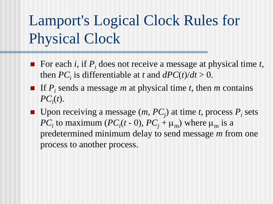
Lamport's Logical Clock Rules for
Physical Clock
For each i, if Pi does not receive a message at physical time t,
then PCi is differentiable at t and dPC(t)/dt > 0.
If Pi sends a message m at physical time t, then m contains
PCi(t).
Upon receiving a message (m, PCj) at time t, process Pi sets
PCi to maximum (PCi(t - 0), PCj + m) where m is a
predetermined minimum delay to send message m from one
process to another process.
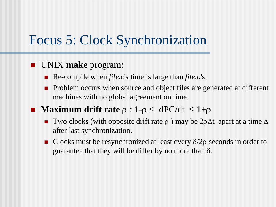
Focus 5: Clock Synchronization
UNIX make program:
Re-compile when file.c's time is large than file.o's.
Problem occurs when source and object files are generated at different
machines with no global agreement on time.
Maximum drift rate : 1- dPC/dt 1+
Two clocks (with opposite drift rate ) may be 2t apart at a time
after last synchronization.
Clocks must be resynchronized at least every /2 seconds in order to
guarantee that they will be differ by no more than .
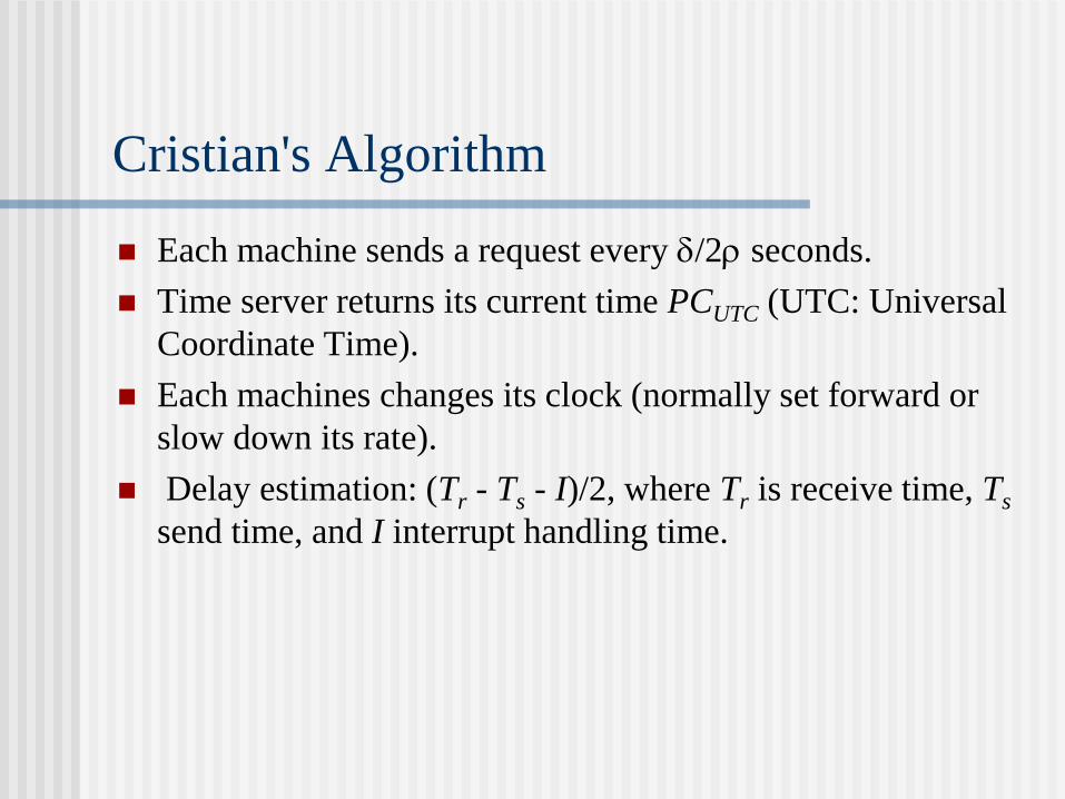
Cristian's Algorithm
Each machine sends a request every /2 seconds.
Time server returns its current time PCUTC (UTC: Universal
Coordinate Time).
Each machines changes its clock (normally set forward or
slow down its rate).
Delay estimation: (Tr - Ts - I)/2, where Tr is receive time, Ts
send time, and I interrupt handling time.
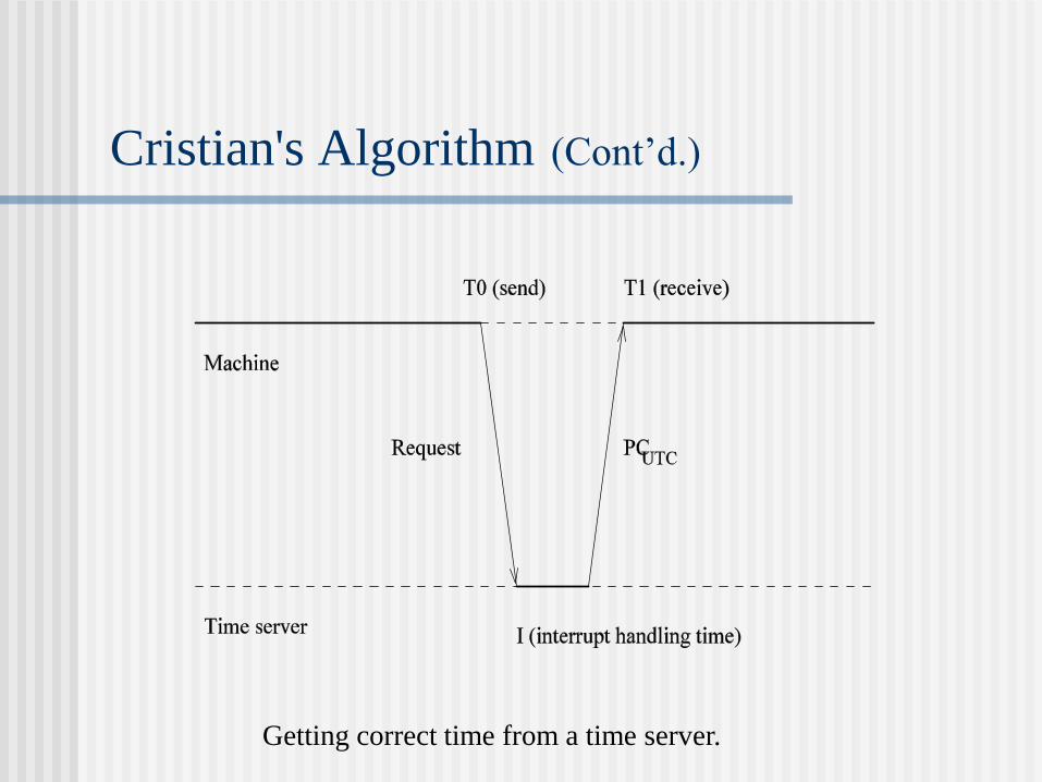
Cristian's Algorithm (Cont’d.)
Getting correct time from a time server.
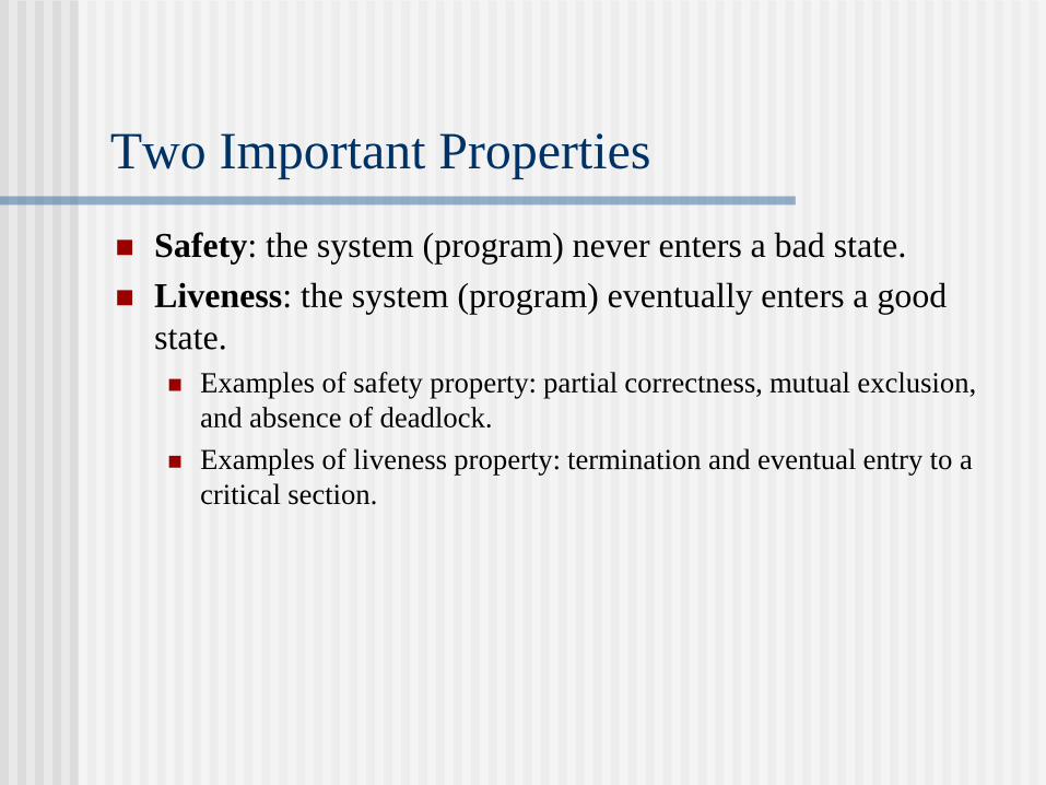
Two Important Properties
Safety: the system (program) never enters a bad state.
Liveness: the system (program) eventually enters a good
state.
Examples of safety property: partial correctness, mutual exclusion,
and absence of deadlock.
Examples of liveness property: termination and eventual entry to a
critical section.
Three Ways to Demonstrate the Properties
Testing and debugging (run the program and see what
happens)
Operational reasoning (exhaustive case analysis)
Assertional reasoning (abstract analysis)
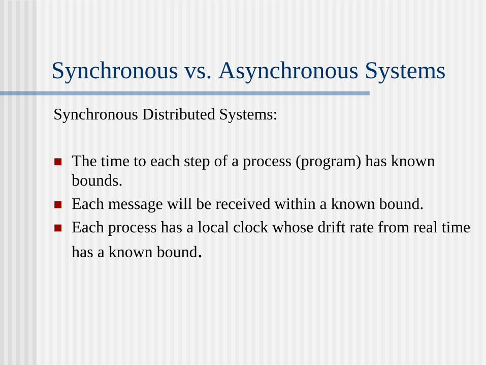
Synchronous vs. Asynchronous Systems
Synchronous Distributed Systems:
The time to each step of a process (program) has known
bounds.
Each message will be received within a known bound.
Each process has a local clock whose drift rate from real time
has a known bound.
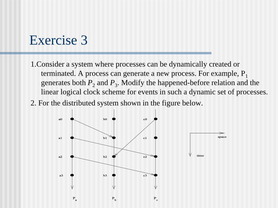
Exercise 3
1.Consider a system where processes can be dynamically created or
terminated. A process can generate a new process. For example, P1
generates both P2 and P3. Modify the happened-before relation and the
linear logical clock scheme for events in such a dynamic set of processes.
2. For the distributed system shown in the figure below.
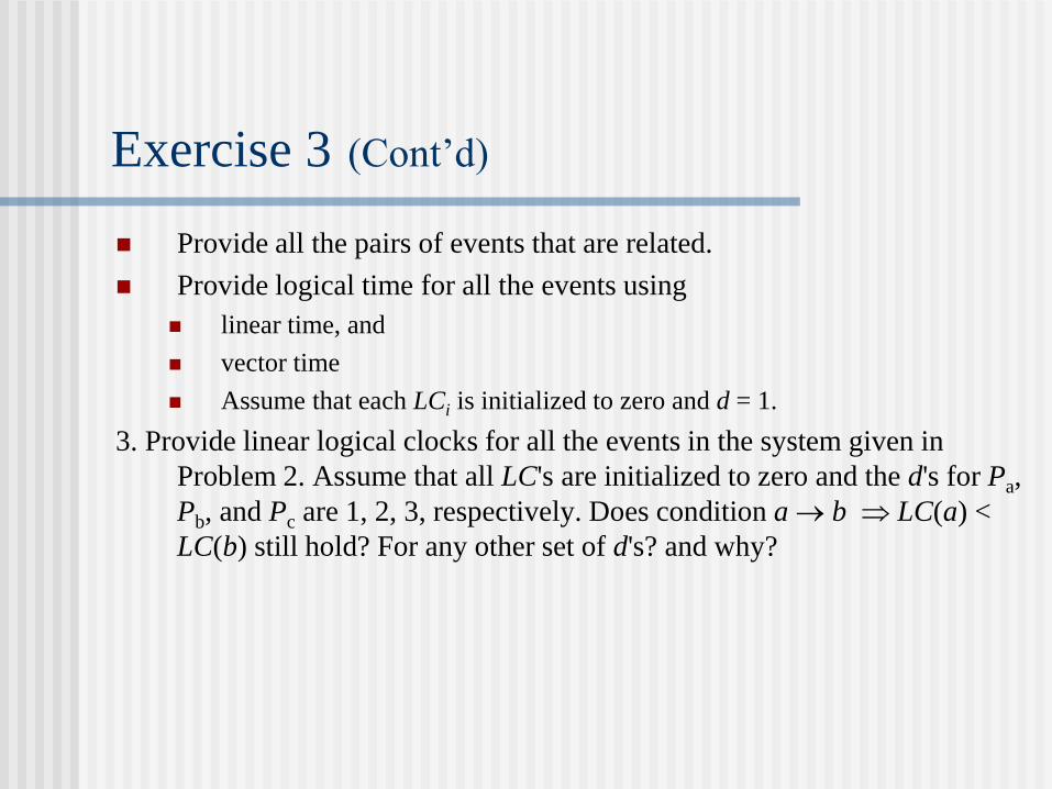
Exercise 3 (Cont’d)
Provide all the pairs of events that are related.
Provide logical time for all the events using
linear time, and
vector time
Assume that each LCi is initialized to zero and d = 1.
3. Provide linear logical clocks for all the events in the system given in
Problem 2. Assume that all LC's are initialized to zero and the d's for Pa,
Pb, and Pc are 1, 2, 3, respectively. Does condition a b LC(a) <
LC(b) still hold? For any other set of d's? and why?
Table of Contents
Introduction and Motivation
Theoretical Foundations
Distributed Programming Languages
Distributed Operating Systems
Distributed Communication
Distributed Data Management
Reliability
Applications
Conclusions
Appendix
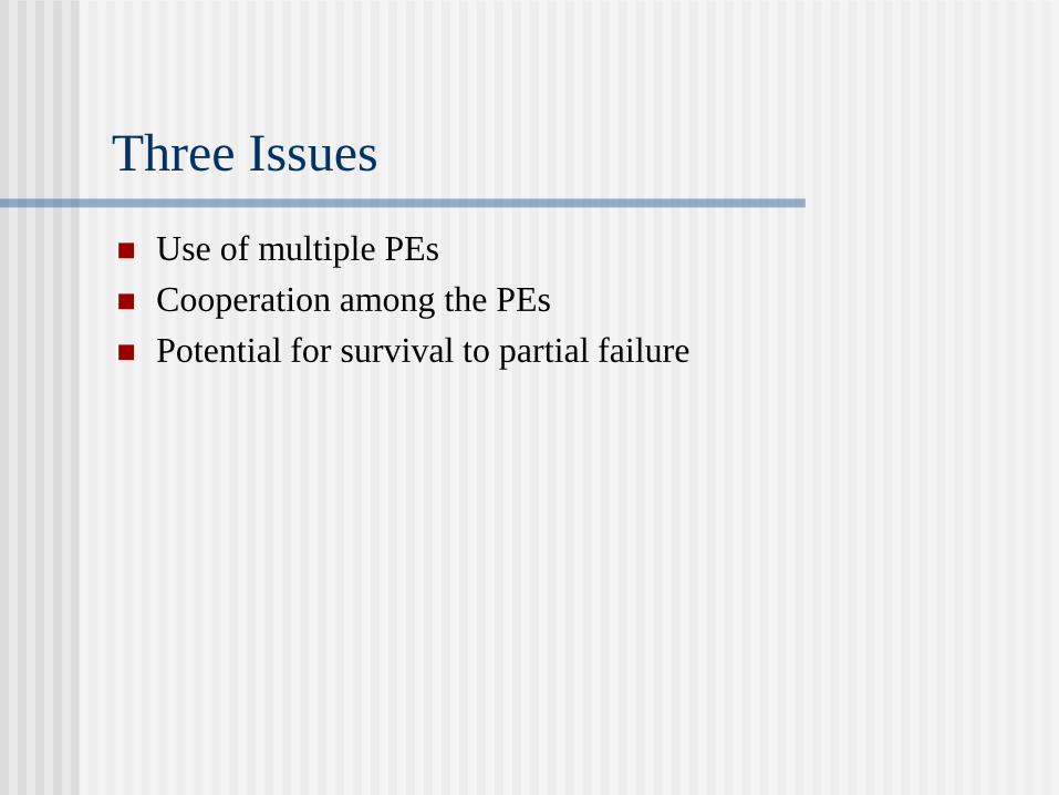
Three Issues
Use of multiple PEs
Cooperation among the PEs
Potential for survival to partial failure

Control Mechanisms
Four basic sequential control mechanisms with
their parallel counterparts.
Statement type \
Control type
Sequential control Parallel Control
Sequential/parallel
statement
Begin S1, S2
end
Parbegin S1, S2
Parend
Fork/join
Alternative statement goto, case if C then
S1 else S2
Guarded commands:
G C
Repetitive statement for … do doall, for all
Subprogram procedure
Subroutine
procedure
subroutine

Focus 6: Expressing Parallelism
A precedence graph of eight statements.
parbegin/parend statement
S1;[[S2;[S3||S4];S5;S6]||S7];S8
Focus 6 (Cont’d.)
fork/join statement
s1;
c1:= 2;
fork L1;
s2;
c2:=2;
fork L2;
s4;
go to L3;
L1: s3;
L2: join c1;
s5;
L3: join c2;
s6;
A precedence graph.
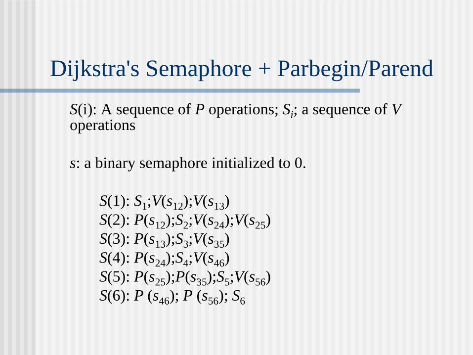
Dijkstra's Semaphore + Parbegin/Parend
S(i): A sequence of P operations; Si; a sequence of V operations
s: a binary semaphore initialized to 0.
S(1): S1;V(s12);V(s13)
S(2): P(s12);S2;V(s24);V(s25)
S(3): P(s13);S3;V(s35)
S(4): P(s24);S4;V(s46)
S(5): P(s25);P(s35);S5;V(s56)
S(6): P (s46); P (s56); S6
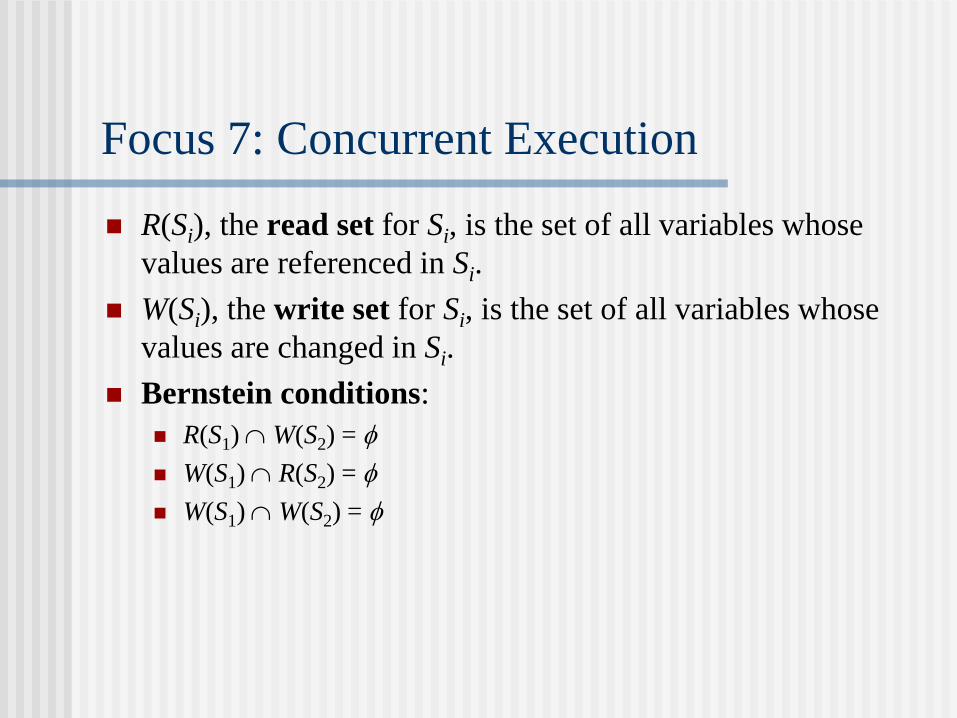
Focus 7: Concurrent Execution
R(Si), the read set for Si, is the set of all variables whose
values are referenced in Si.
W(Si), the write set for Si, is the set of all variables whose
values are changed in Si.
Bernstein conditions:
R(S1) W(S2) =
W(S1) R(S2) =
W(S1) W(S2) =
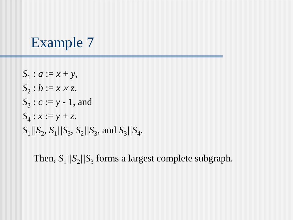
Example 7
S1 : a := x + y,
S2 : b := x z,
S3 : c := y - 1, and
S4 : x := y + z.
S1||S2, S1||S3, S2||S3, and S3||S4.
Then, S1||S2||S3 forms a largest complete subgraph.
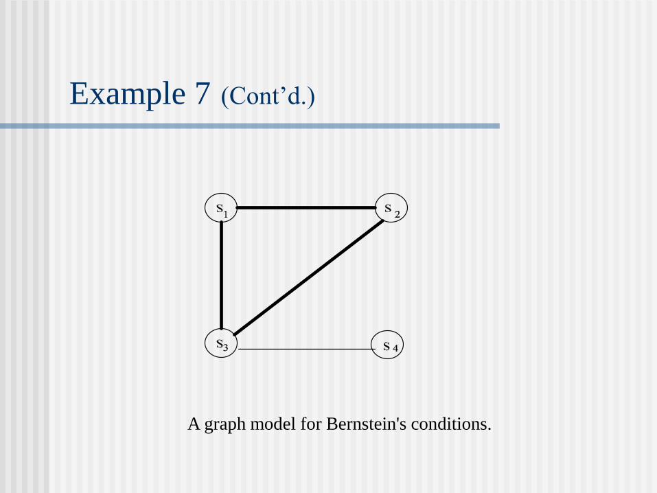
Example 7 (Cont’d.)
A graph model for Bernstein's conditions.
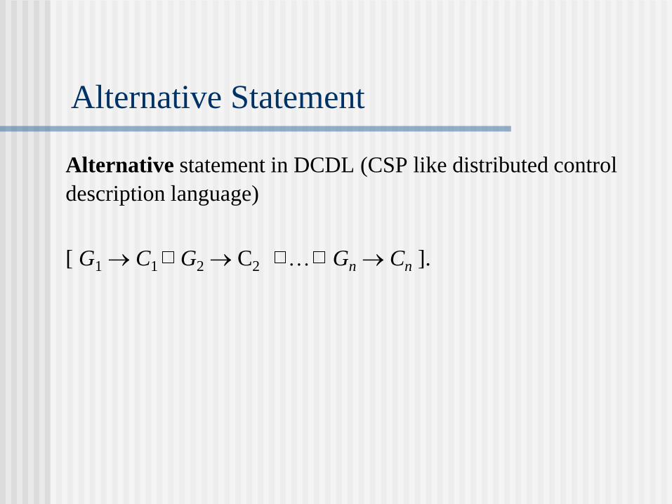
Alternative statement in DCDL (CSP like distributed control
description language)
[ G1 C1 G2 C2 … Gn Cn ].
Alternative Statement
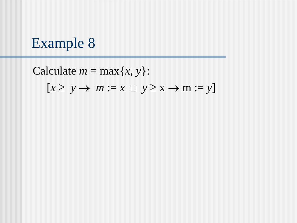
Calculate m = max{x, y}:
[x y m := x y x m := y]
Example 8
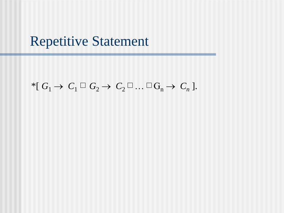
Repetitive Statement
*[ G1 C1 G2 C2 … Gn Cn ].
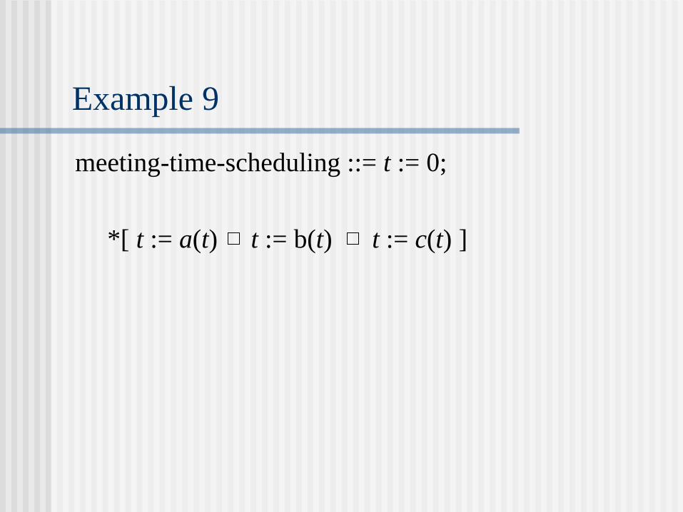
Example 9
meeting-time-scheduling ::= t := 0;
*[ t := a(t) t := b(t) t := c(t) ]
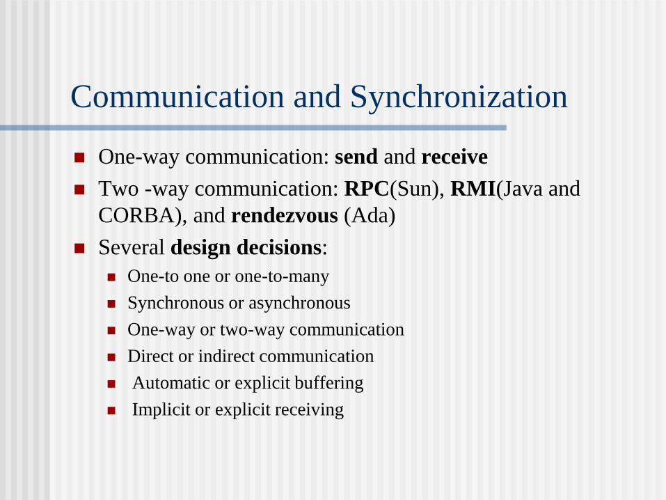
Communication and Synchronization
One-way communication: send and receive
Two -way communication: RPC(Sun), RMI(Java and
CORBA), and rendezvous (Ada)
Several design decisions:
One-to one or one-to-many
Synchronous or asynchronous
One-way or two-way communication
Direct or indirect communication
Automatic or explicit buffering
Implicit or explicit receiving
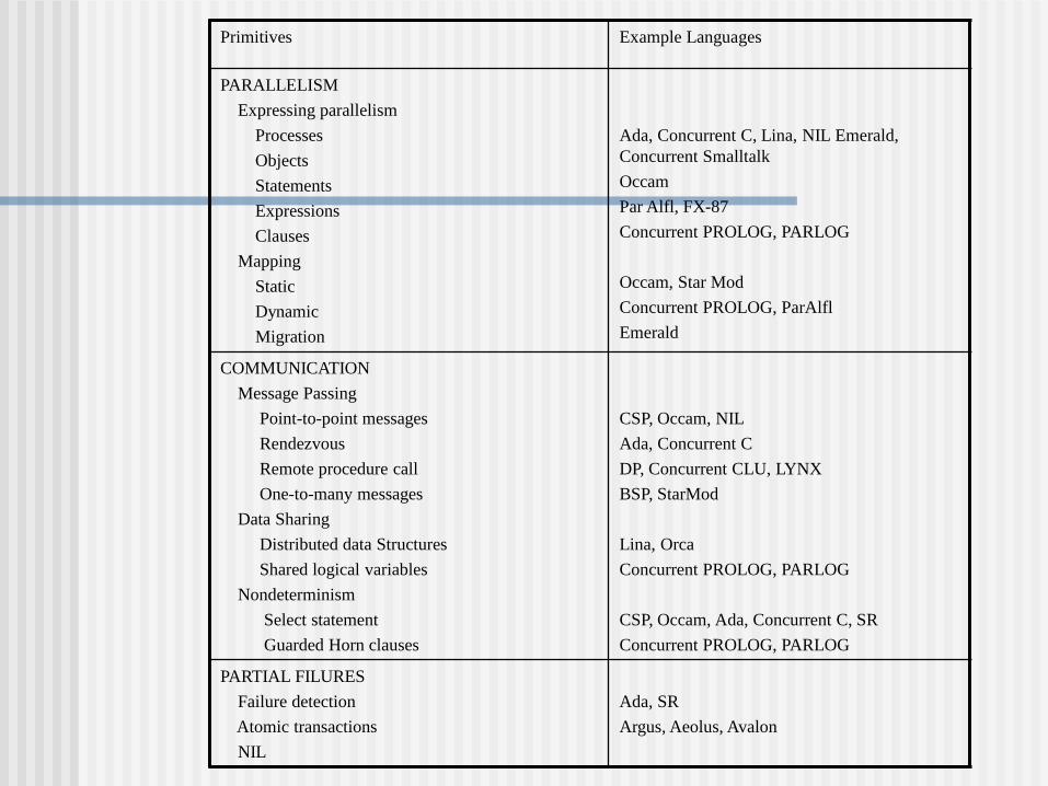
Primitives Example Languages
PARALLELISM
Expressing parallelism
Processes
Objects
Statements
Expressions
Clauses
Mapping
Static
Dynamic
Migration
Ada, Concurrent C, Lina, NIL Emerald,
Concurrent Smalltalk
Occam
Par Alfl, FX-87
Concurrent PROLOG, PARLOG
Occam, Star Mod
Concurrent PROLOG, ParAlfl
Emerald
COMMUNICATION
Message Passing
Point-to-point messages
Rendezvous
Remote procedure call
One-to-many messages
Data Sharing
Distributed data Structures
Shared logical variables
Nondeterminism
Select statement
Guarded Horn clauses
CSP, Occam, NIL
Ada, Concurrent C
DP, Concurrent CLU, LYNX
BSP, StarMod
Lina, Orca
Concurrent PROLOG, PARLOG
CSP, Occam, Ada, Concurrent C, SR
Concurrent PROLOG, PARLOG
PARTIAL FILURES
Failure detection
Atomic transactions
NIL
Ada, SR
Argus, Aeolus, Avalon
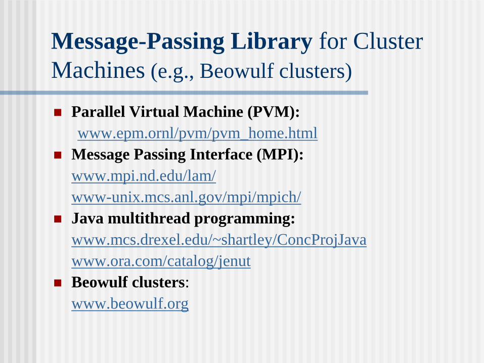
Message-Passing Library for Cluster
Machines (e.g., Beowulf clusters)
Parallel Virtual Machine (PVM):
www.epm.ornl/pvm/pvm_home.html
Message Passing Interface (MPI):
www.mpi.nd.edu/lam/
www-unix.mcs.anl.gov/mpi/mpich/
Java multithread programming:
www.mcs.drexel.edu/~shartley/ConcProjJava
www.ora.com/catalog/jenut
Beowulf clusters:
www.beowulf.org
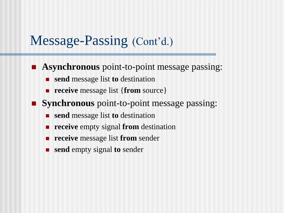
Message-Passing (Cont’d.)
Asynchronous point-to-point message passing:
send message list to destination
receive message list {from source}
Synchronous point-to-point message passing:
send message list to destination
receive empty signal from destination
receive message list from sender
send empty signal to sender
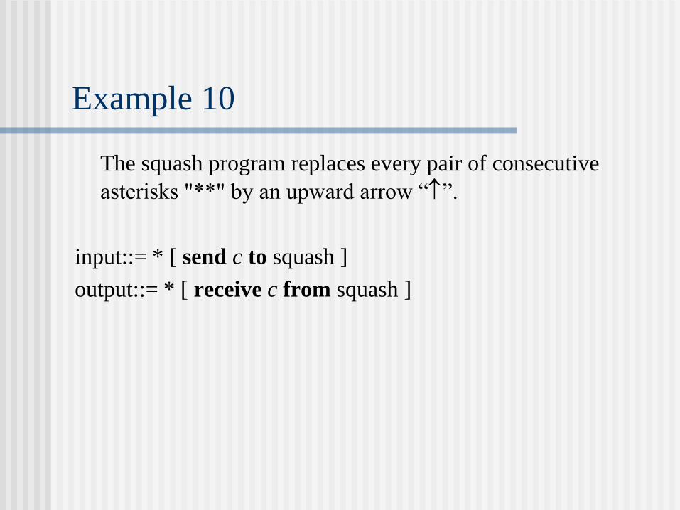
Example 10
The squash program replaces every pair of consecutive
asterisks "**" by an upward arrow “”.
input::= * [ send c to squash ]
output::= * [ receive c from squash ]
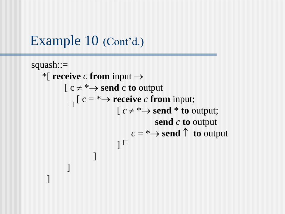
Example 10 (Cont’d.)
squash::=
*[ receive c from input
[ c * send c to output
[ c = * receive c from input;
[ c * send * to output;
send c to output
c = * send to output
]
]
]
]
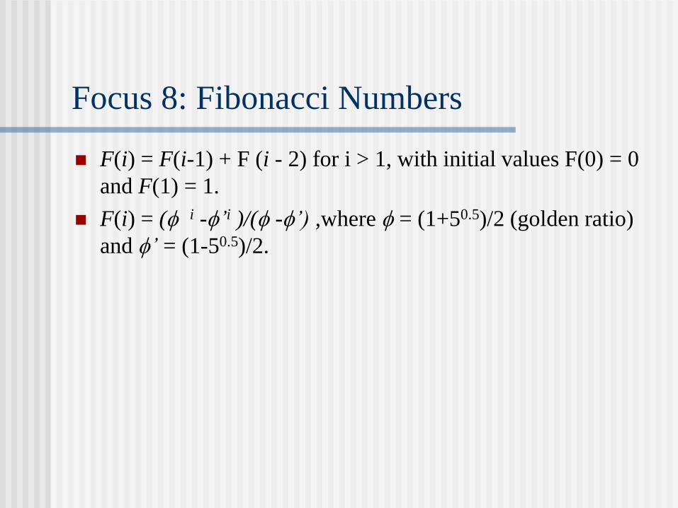
Focus 8: Fibonacci Numbers
F(i) = F(i-1) + F (i - 2) for i > 1, with initial values F(0) = 0
and F(1) = 1.
F(i) = ( i -’i )/( -’) ,where = (1+50.5)/2 (golden ratio)
and ’ = (1-50.5)/2.
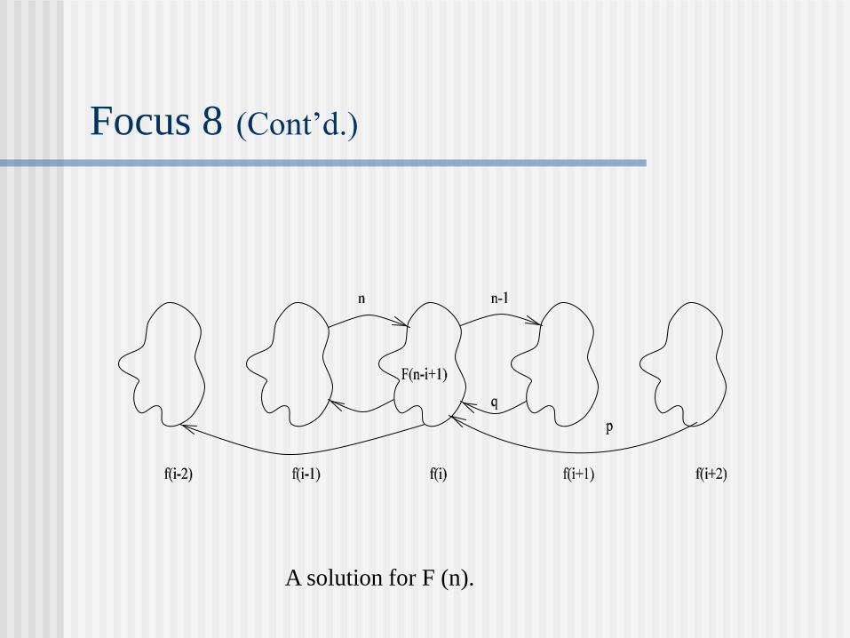
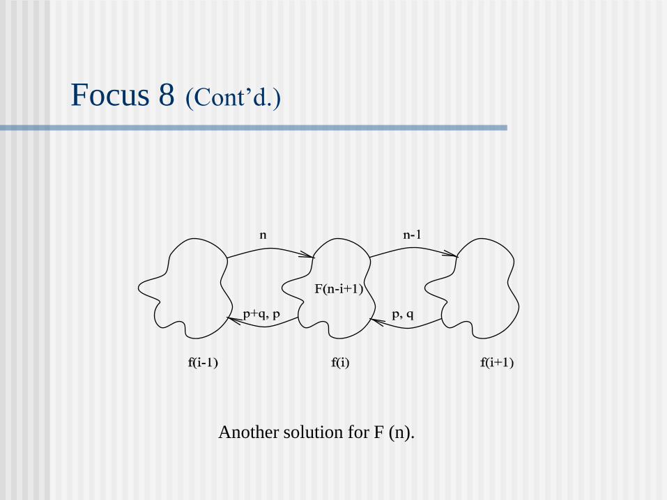
Focus 8 (Cont’d.)
A solution for F (n).

Focus 8 (Cont’d.)
f(0) ::=
send n to f(1);
receive p from f(2);
receive q from f(1);
ans := q
f(-1) ::=
receive p from f(1)

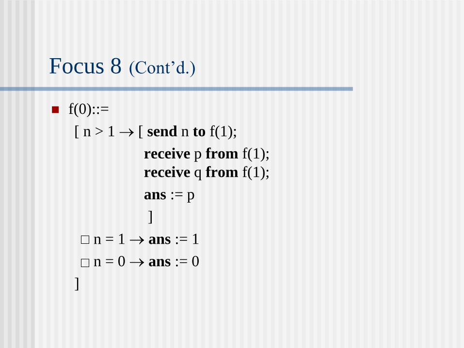
Focus 8 (Cont’d.)
f(i) ::=
receive n from f(i - 1);
[ n > 1 [ send n - 1 to f(i + 1);
receive p from f(i + 2);
receive q from f(i + 1);
send p + q to f(i - 1);
send p + q to f(i - 2) ]
n = 1 [ send 1 to f(i - 1);
send 1 to f(i - 2) ]
n = 0 [ send 0 to f(i - 1);
send 0 to f(i - 2) ]
]
Another solution for F (n).
Focus 8 (Cont’d.)
f(0)::=
[ n > 1 [ send n to f(1);
receive p from f(1);
receive q from f(1);
ans := p
]
n = 1 ans := 1
n = 0 ans := 0
]
Focus 8 (Cont’d.)
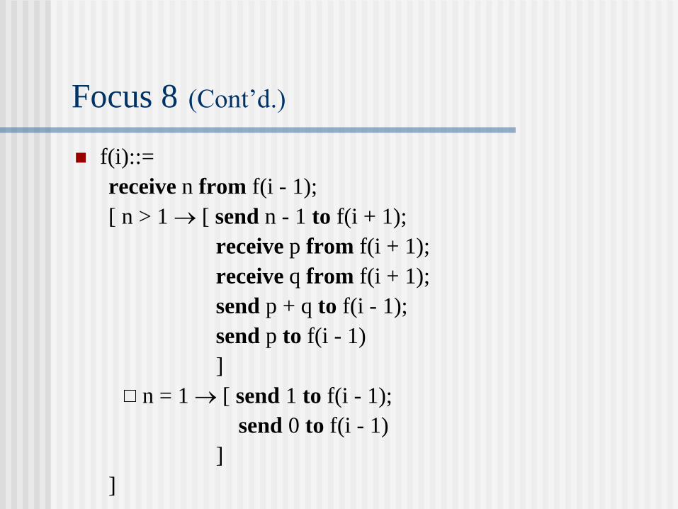
f(i)::=
receive n from f(i - 1);
[ n > 1 [ send n - 1 to f(i + 1);
receive p from f(i + 1);
receive q from f(i + 1);
send p + q to f(i - 1);
send p to f(i - 1)
]
n = 1 [ send 1 to f(i - 1);
send 0 to f(i - 1)
]
]
Focus 8 (Cont’d.)
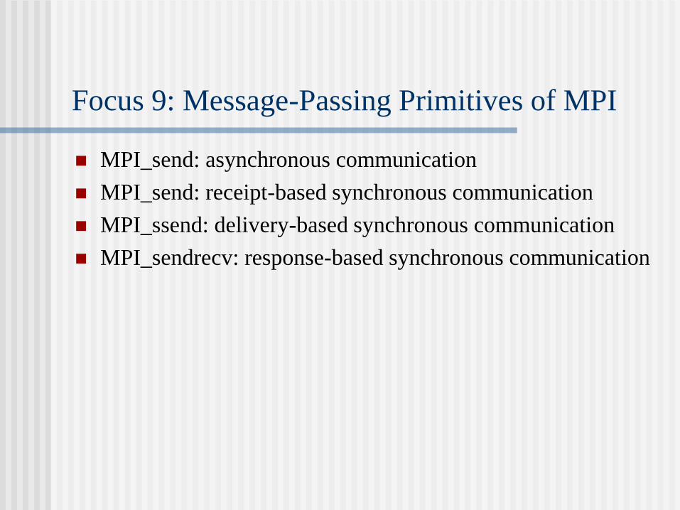
Focus 9: Message-Passing Primitives of MPI
MPI_send: asynchronous communication
MPI_send: receipt-based synchronous communication
MPI_ssend: delivery-based synchronous communication
MPI_sendrecv: response-based synchronous communication
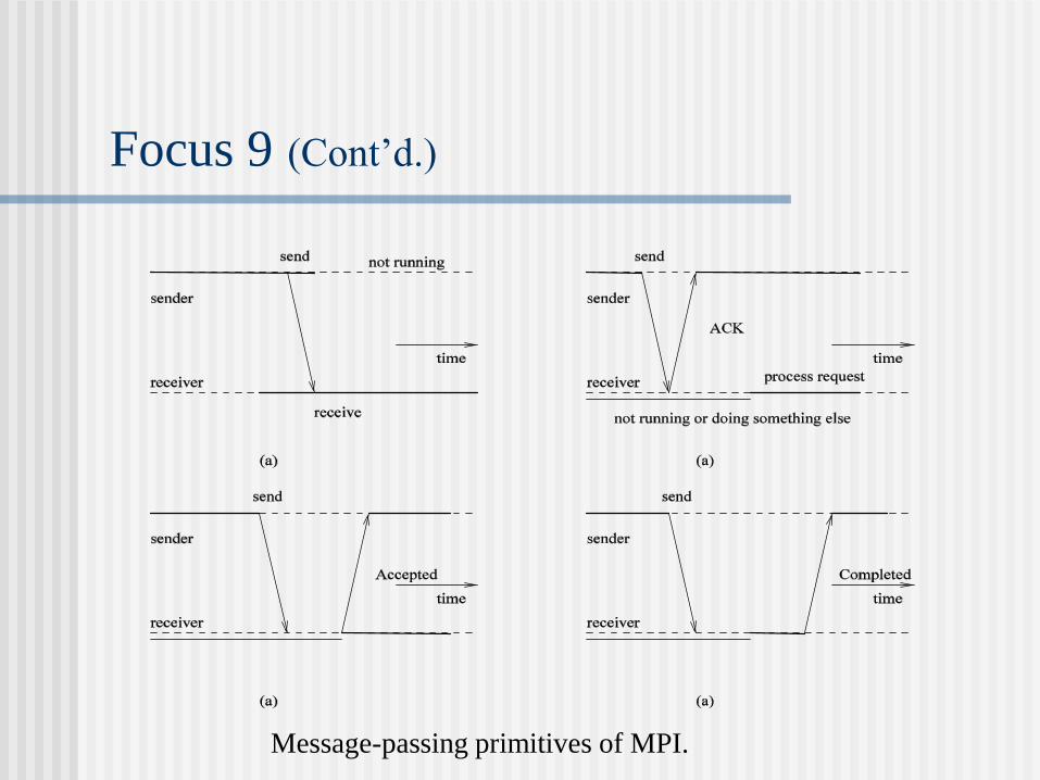
Focus 9 (Cont’d.)
Message-passing primitives of MPI.
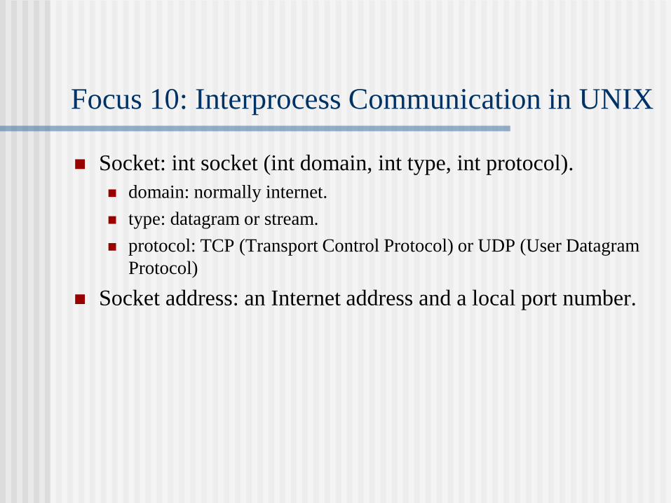
Focus 10: Interprocess Communication in UNIX
Socket: int socket (int domain, int type, int protocol).
domain: normally internet.
type: datagram or stream.
protocol: TCP (Transport Control Protocol) or UDP (User Datagram
Protocol)
Socket address: an Internet address and a local port number.
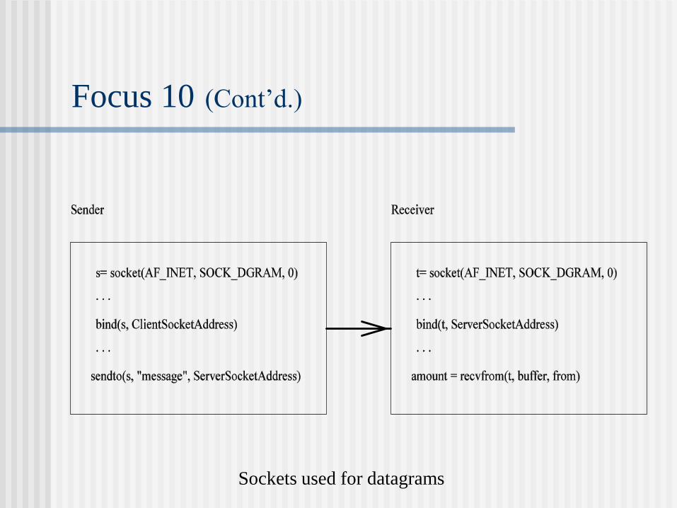
Focus 10 (Cont’d.)
Sockets used for datagrams
High-Level (Middleware) Communication
Services
Achieve access transparency in distributed systems
Remote procedure call (RPC)
Remote method invocation (RMI)
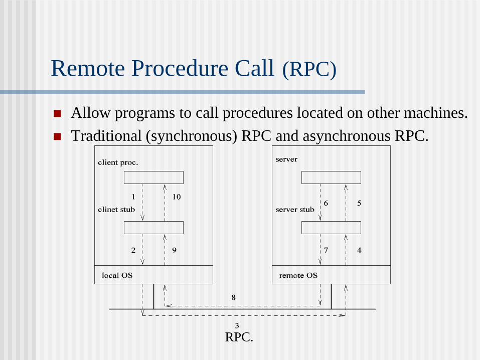
Remote Procedure Call (RPC)
Allow programs to call procedures located on other machines.
Traditional (synchronous) RPC and asynchronous RPC.
RPC.
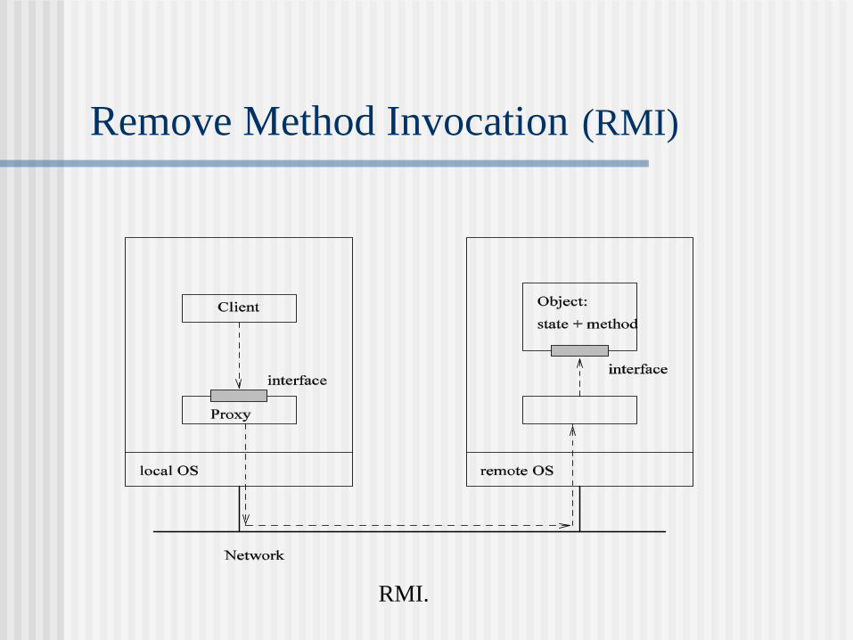
Remove Method Invocation (RMI)
RMI.
Robustness
Exception handling in high level languages (Ada and
PL/1)
Four Types of Communication Faults
A message transmitted from a node does not reach its
intended destinations
Messages are not received in the same order as they were
sent
A message gets corrupted during its transmission
A message gets replicated during its transmission
If a remote procedure call terminates abnormally
(the time out expires) there are four possibilities.
The receiver did not receive the call message.
The reply message did not reach the sender.
The receiver crashed during the call execution and either
has remained crashed or is not resuming the execution
after crash recovery.
The receiver is still executing the call, in which case the
execution could interfere with subsequent activities of the
client.
Failures in RPC

Exercise 2
1.(The Welfare Crook by W. Feijen) Suppose we have three
long magnetic tapes each containing a list of names in
alphabetical order. The first list contains the names of people
working at IBM Yorktown, the second the names of students
at Columbia University and the third the names of all people
on welfare in New York City. All three lists are endless so no
upper bounds are given. It is known that at least one person is
on all three lists. Write a program to locate the first such
person (the one with the alphabetically smallest name). Your
solution should use three processes, one for each tape.
Exercise 2 (Cont’d.)
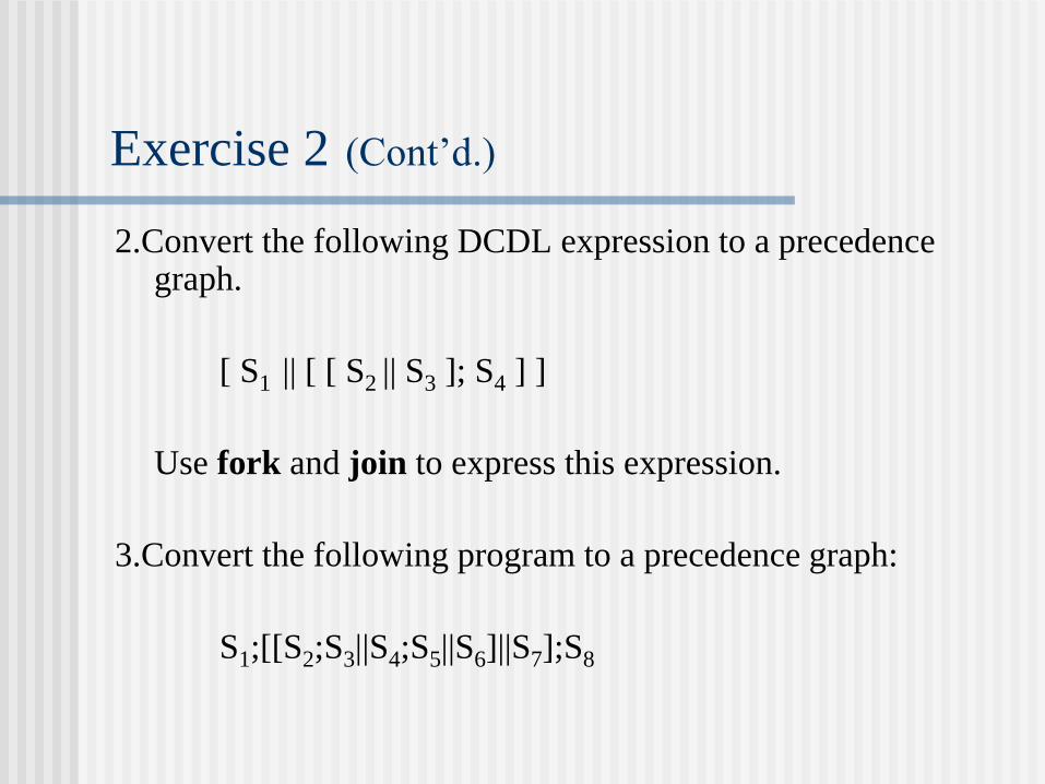
2.Convert the following DCDL expression to a precedence graph.
[ S1 || [ [ S2 || S3 ]; S4 ] ]
Use fork and join to express this expression.
3.Convert the following program to a precedence graph:
S1;[[S2;S3||S4;S5||S6]||S7];S8
Exercise 2 (Cont’d.)
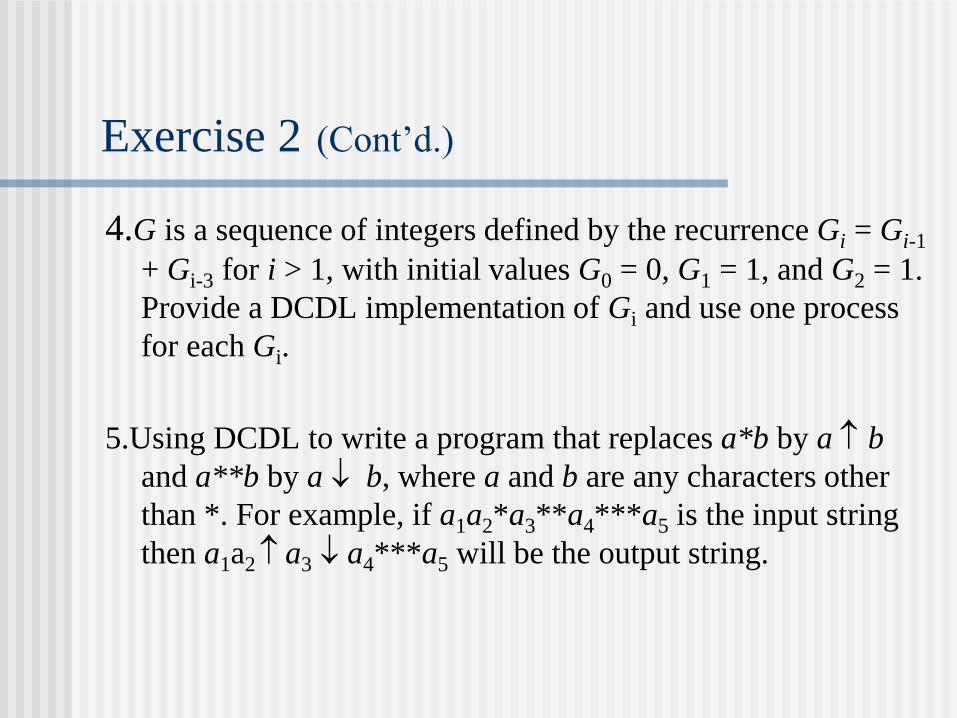
4.G is a sequence of integers defined by the recurrence Gi = Gi-1
+ Gi-3 for i > 1, with initial values G0 = 0, G1 = 1, and G2 = 1.
Provide a DCDL implementation of Gi and use one process
for each Gi.
5.Using DCDL to write a program that replaces a*b by a b
and a**b by a b, where a and b are any characters other
than *. For example, if a1a2*a3**a4***a5 is the input string
then a1a2 a3 a4***a5 will be the output string.

Table of Contents
Introduction and Motivation
Theoretical Foundations
Distributed Programming Languages
Distributed Operating Systems
Distributed Communication
Distributed Data Management
Reliability
Applications
Conclusions
Appendix
Distributed Operating Systems
Operating Systems: provide problem-oriented abstractions of
the underlying physical resources.
Files (rather than disk blocks) and sockets (rather than raw
network access).
Selected Issues
Mutual exclusion and election Non-token-based vs. token-based
Election and bidding
Detection and resolution of deadlock Four conditions for deadlock: mutual exclusion, hold and wait, no
preemption, and circular wait.
Graph-theoretic model: wait-for graph
Two situations: AND model (process deadlock) and OR model (communication deadlock)
Task scheduling and load balancing Static scheduling vs. dynamic scheduling
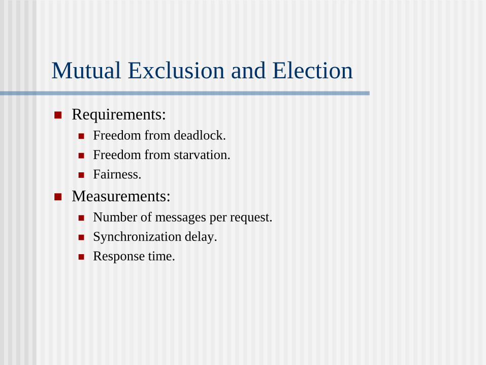
Mutual Exclusion and Election
Requirements:
Freedom from deadlock.
Freedom from starvation.
Fairness.
Measurements:
Number of messages per request.
Synchronization delay.
Response time.
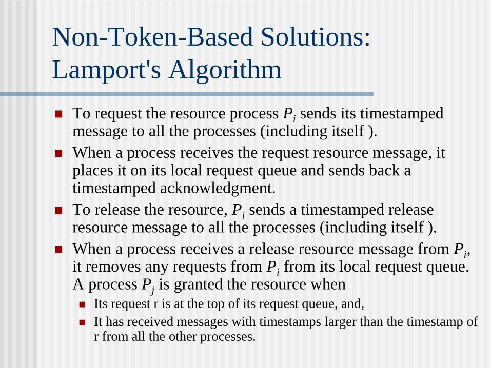
Non-Token-Based Solutions:
Lamport's Algorithm
To request the resource process Pi sends its timestamped message to all the processes (including itself ).
When a process receives the request resource message, it places it on its local request queue and sends back a timestamped acknowledgment.
To release the resource, Pi sends a timestamped release resource message to all the processes (including itself ).
When a process receives a release resource message from Pi, it removes any requests from Pi from its local request queue. A process Pj is granted the resource when
Its request r is at the top of its request queue, and,
It has received messages with timestamps larger than the timestamp of r from all the other processes.

Example for Lamport’s Algorithm
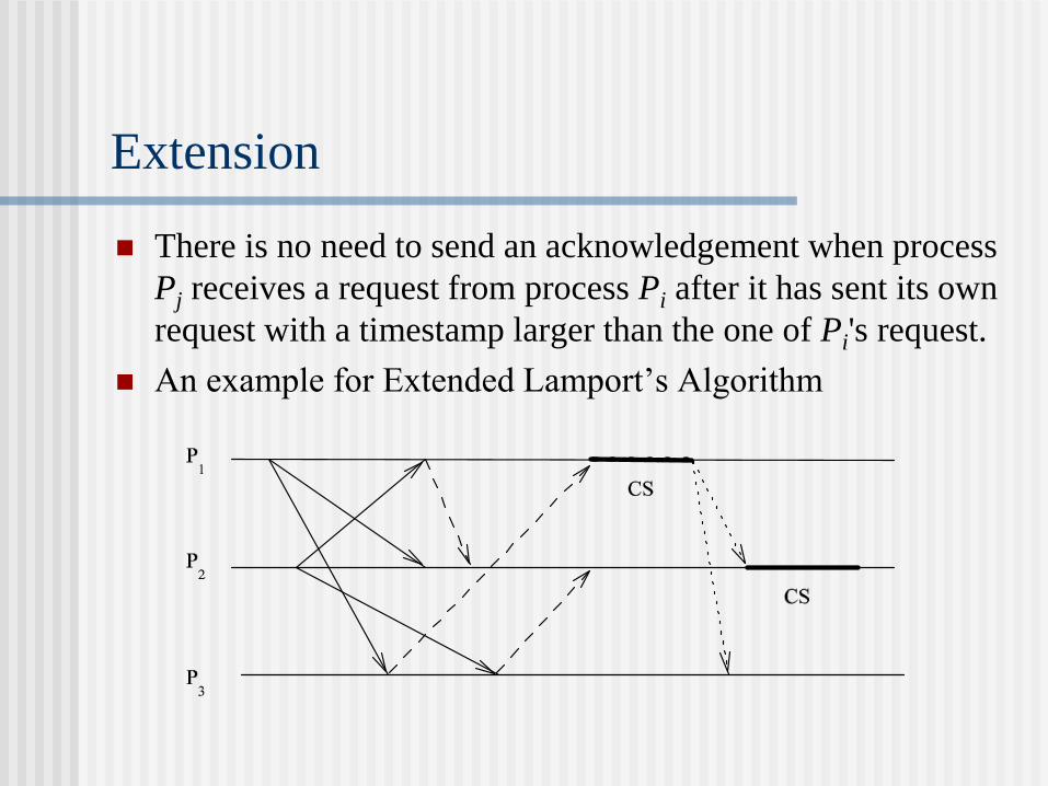
Extension
There is no need to send an acknowledgement when process
Pj receives a request from process Pi after it has sent its own
request with a timestamp larger than the one of Pi's request.
An example for Extended Lamport’s Algorithm
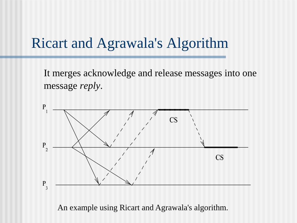
Ricart and Agrawala's Algorithm
It merges acknowledge and release messages into one
message reply.
An example using Ricart and Agrawala's algorithm.

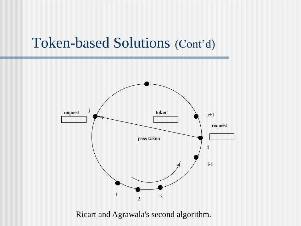
Token-Based Solutions: Ricart and
Agrawala's Second Algorithm
When token holder Pi exits CS, it searches other processes in
the order i + 1,i + 2,…,n,1,2,…,i - 1 for the first j such that
the timestamp of Pj 's last request for the token is larger than
the value recorded in the token for the timestamp of Pj 's last
holding of the token.
Token-based Solutions (Cont’d)
Ricart and Agrawala's second algorithm.
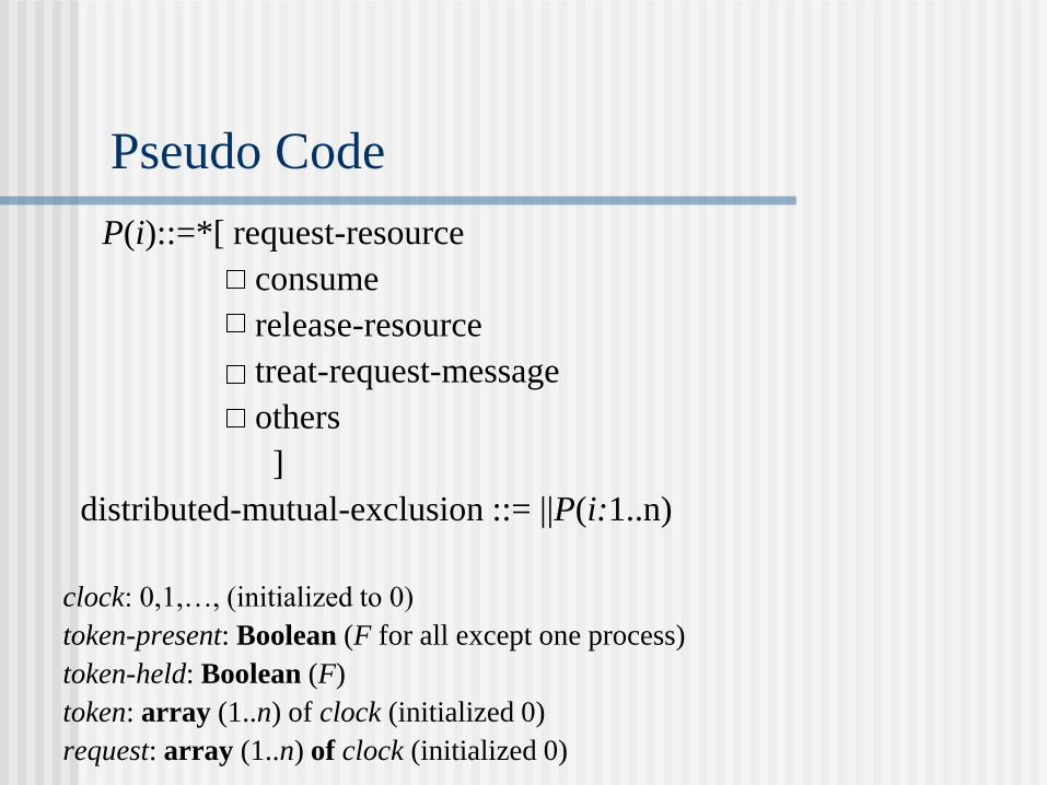
P(i)::=*[ request-resource
consume
release-resource
treat-request-message
others
]
distributed-mutual-exclusion ::= ||P(i:1..n)
clock: 0,1,…, (initialized to 0)
token-present: Boolean (F for all except one process)
token-held: Boolean (F)
token: array (1..n) of clock (initialized 0)
request: array (1..n) of clock (initialized 0)
Pseudo Code
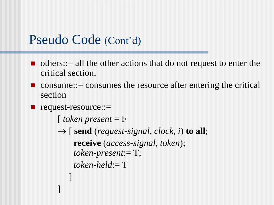
others::= all the other actions that do not request to enter the critical section.
consume::= consumes the resource after entering the critical section
request-resource::=
[ token present = F
[ send (request-signal, clock, i) to all;
receive (access-signal, token); token-present:= T;
token-held:= T
]
]
Pseudo Code (Cont’d)

release-resource::=
[ token (i):=clock;
token-held:= F;
min j in the order [i + 1,… n,1,2,…,i – 2, i – 1]
(request(j) > token(j))
[ token-present:= F;
send (access-signal, token) to Pj
]
]
Pseudo Code (Cont’d)
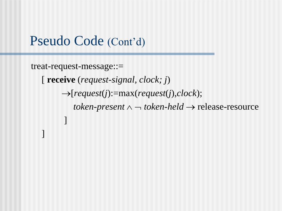
treat-request-message::=
[ receive (request-signal, clock; j)
[request(j):=max(request(j),clock);
token-present token-held release-resource
]
]
Pseudo Code (Cont’d)
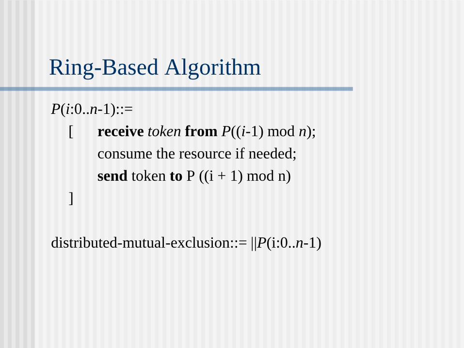
Ring-Based Algorithm
P(i:0..n-1)::=
[ receive token from P((i-1) mod n);
consume the resource if needed;
send token to P ((i + 1) mod n)
]
distributed-mutual-exclusion::= ||P(i:0..n-1)

Ring-Based Algorithm (Cont’d)
The simple token-ring-based algorithm (a) and the
fault-tolerant token-ring-based algorithm (b).
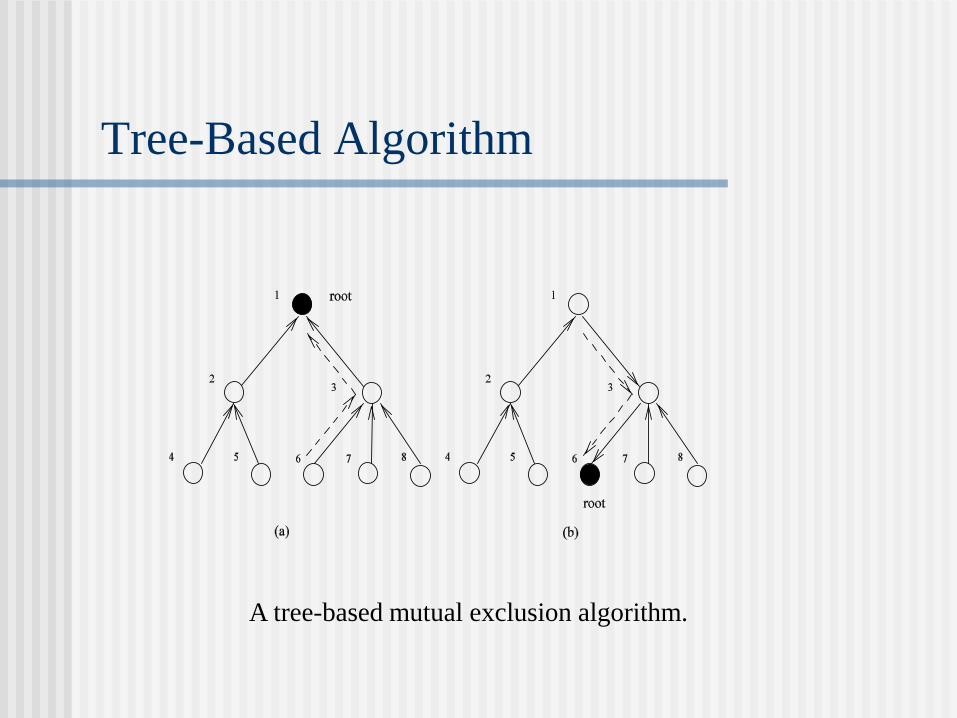
Tree-Based Algorithm
A tree-based mutual exclusion algorithm.

Maekawa's Algorithm
Permission from every other process but only from a
subset of processes.
If Ri and Rj are the request sets for processes Pi and
Pj , then Ri Rj .
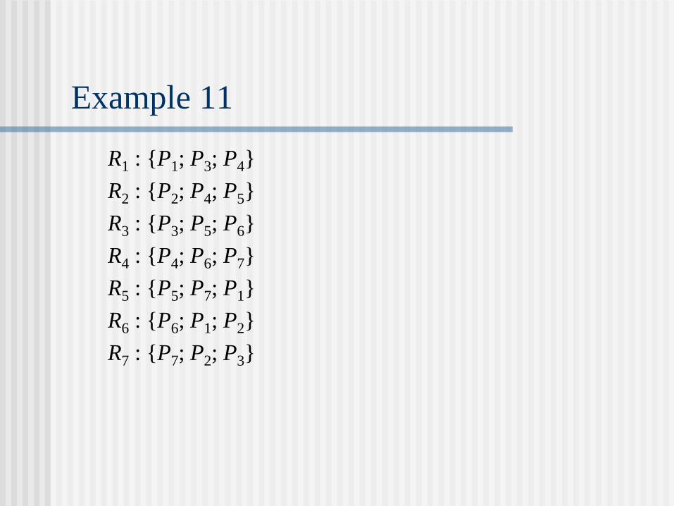
Example 11
R1 : {P1; P3; P4}
R2 : {P2; P4; P5}
R3 : {P3; P5; P6}
R4 : {P4; P6; P7}
R5 : {P5; P7; P1}
R6 : {P6; P1; P2}
R7 : {P7; P2; P3}
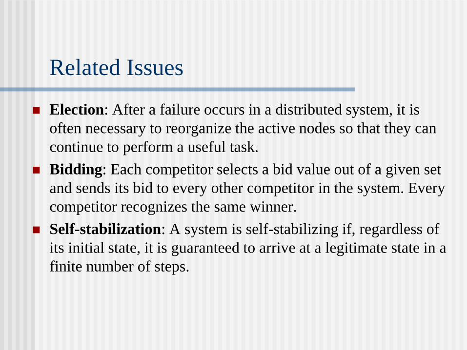
Related Issues
Election: After a failure occurs in a distributed system, it is
often necessary to reorganize the active nodes so that they can
continue to perform a useful task.
Bidding: Each competitor selects a bid value out of a given set
and sends its bid to every other competitor in the system. Every
competitor recognizes the same winner.
Self-stabilization: A system is self-stabilizing if, regardless of
its initial state, it is guaranteed to arrive at a legitimate state in a
finite number of steps.
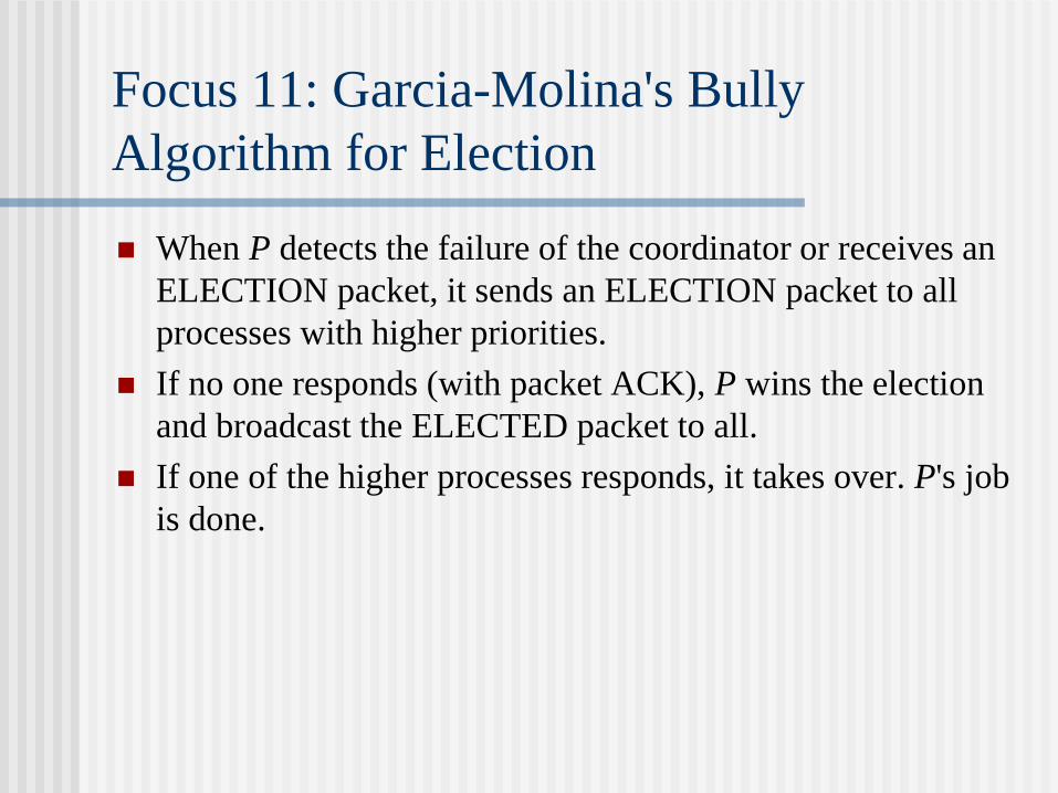
Focus 11: Garcia-Molina's Bully
Algorithm for Election
When P detects the failure of the coordinator or receives an
ELECTION packet, it sends an ELECTION packet to all
processes with higher priorities.
If no one responds (with packet ACK), P wins the election
and broadcast the ELECTED packet to all.
If one of the higher processes responds, it takes over. P's job
is done.
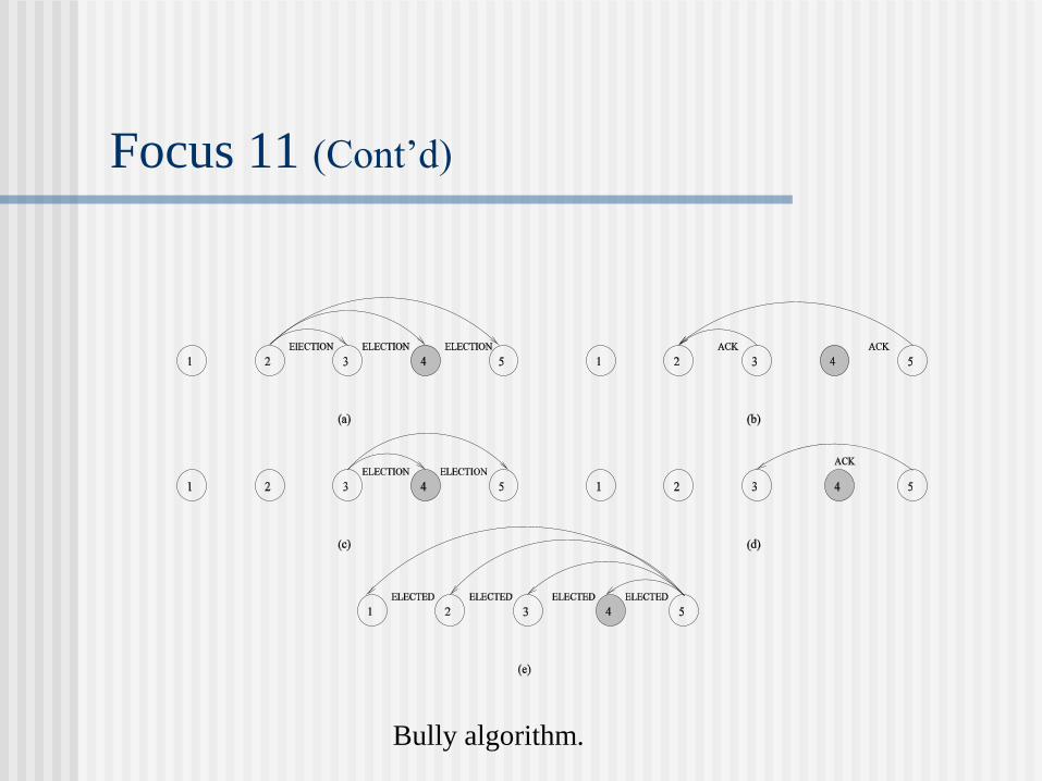
Focus 11 (Cont’d)
Bully algorithm.
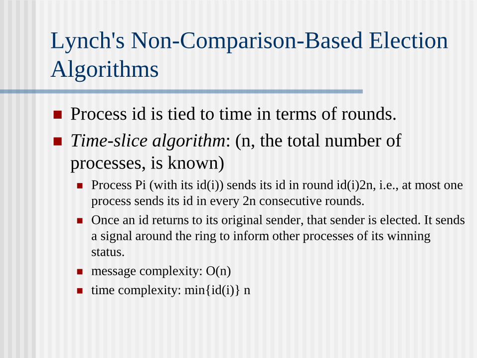
Lynch's Non-Comparison-Based Election
Algorithms
Process id is tied to time in terms of rounds.
Time-slice algorithm: (n, the total number of
processes, is known) Process Pi (with its id(i)) sends its id in round id(i)2n, i.e., at most one
process sends its id in every 2n consecutive rounds.
Once an id returns to its original sender, that sender is elected. It sends
a signal around the ring to inform other processes of its winning
status.
message complexity: O(n)
time complexity: min{id(i)} n
Variable-speed algorithm: (n is unknown)
When a process Pi sends its id (id(i)), this id travels at
the rate of one transmission for every 2id(i) rounds.
If an id returns to its original sender, that sender is
elected.
message complexity: n + n/2 + n/22 + … + n/2(n-1)
< 2n = O(n)
time complexity: 2 min{id(i)}n
Lynch's Algorithms (Cont’d)
Dijkstra's Self-Stabilization
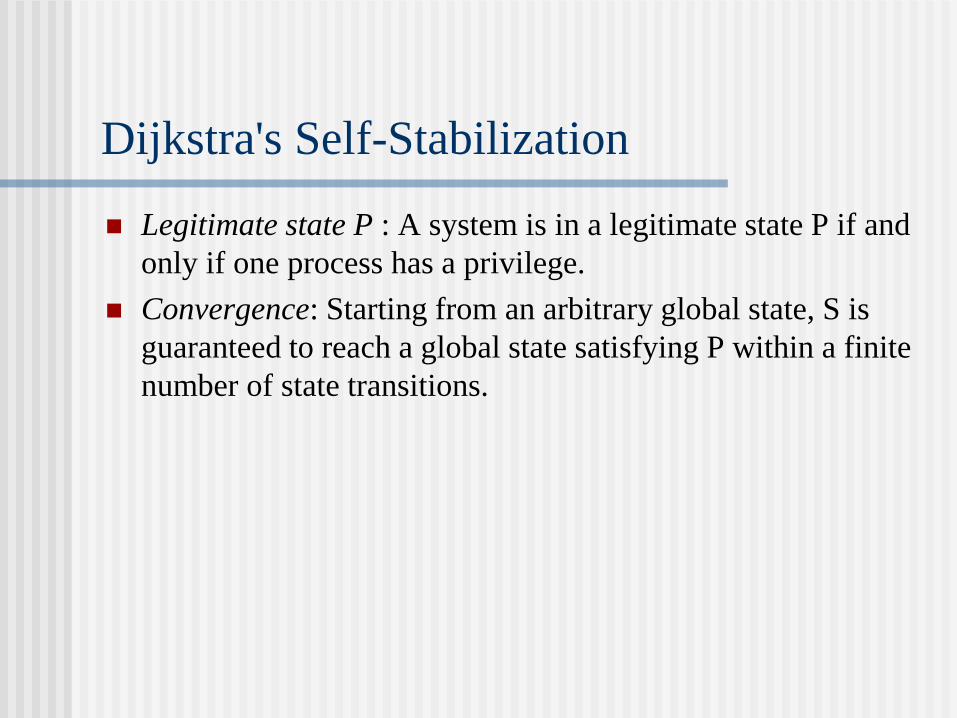
Legitimate state P : A system is in a legitimate state P if and
only if one process has a privilege.
Convergence: Starting from an arbitrary global state, S is
guaranteed to reach a global state satisfying P within a finite
number of state transitions.
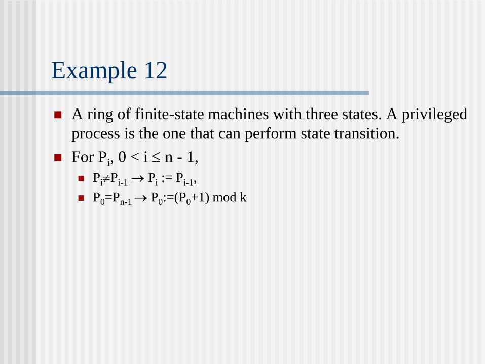
Example 12
A ring of finite-state machines with three states. A privileged
process is the one that can perform state transition.
For Pi, 0 < i n - 1,
PiPi-1 Pi := Pi-1,
P0=Pn-1 P0:=(P0+1) mod k
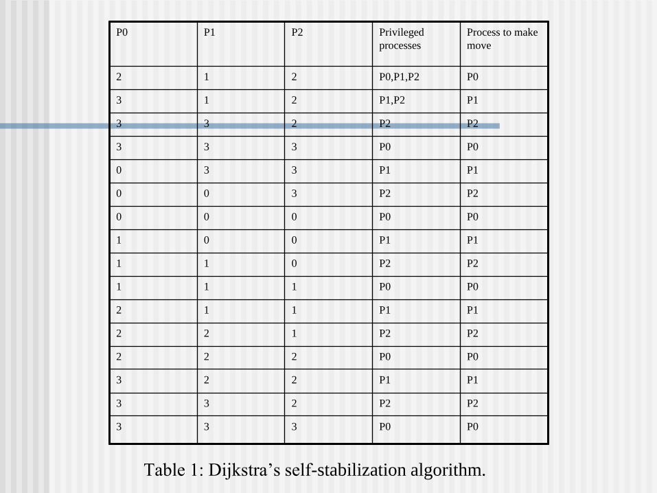
Table 1: Dijkstra’s self-stabilization algorithm.
P0 P1 P2 Privileged
processes
Process to make
move
2 1 2 P0,P1,P2 P0
3 1 2 P1,P2 P1
3 3 2 P2 P2
3 3 3 P0 P0
0 3 3 P1 P1
0 0 3 P2 P2
0 0 0 P0 P0
1 0 0 P1 P1
1 1 0 P2 P2
1 1 1 P0 P0
2 1 1 P1 P1
2 2 1 P2 P2
2 2 2 P0 P0
3 2 2 P1 P1
3 3 2 P2 P2
3 3 3 P0 P0
Extensions
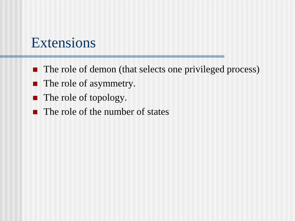
The role of demon (that selects one privileged process)
The role of asymmetry.
The role of topology.
The role of the number of states
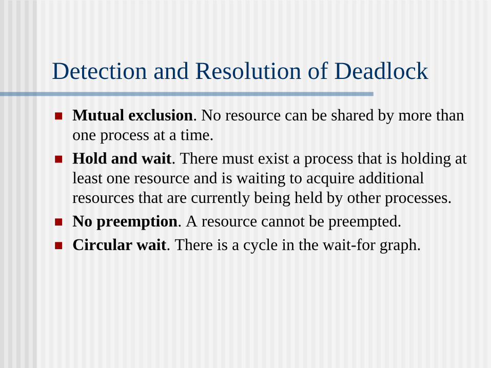
Detection and Resolution of Deadlock
Mutual exclusion. No resource can be shared by more than
one process at a time.
Hold and wait. There must exist a process that is holding at
least one resource and is waiting to acquire additional
resources that are currently being held by other processes.
No preemption. A resource cannot be preempted.
Circular wait. There is a cycle in the wait-for graph.
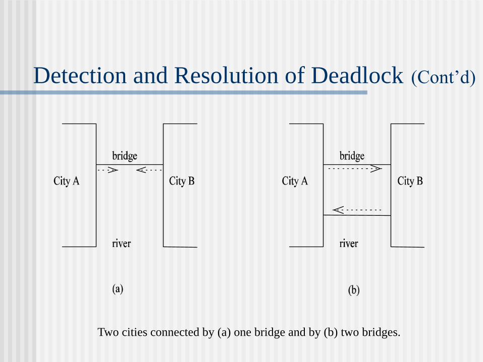
Detection and Resolution of Deadlock (Cont’d)
Two cities connected by (a) one bridge and by (b) two bridges.
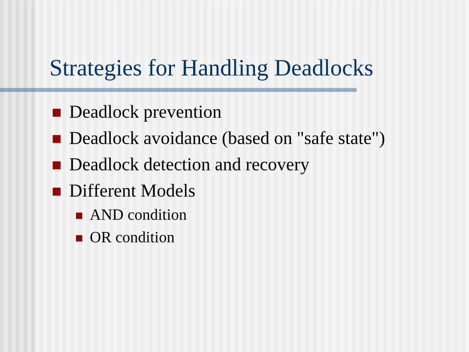
Strategies for Handling Deadlocks
Deadlock prevention
Deadlock avoidance (based on "safe state")
Deadlock detection and recovery
Different Models
AND condition
OR condition
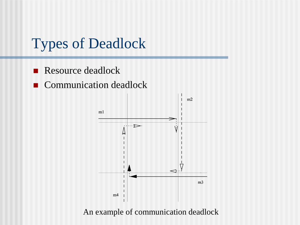
Types of Deadlock
Resource deadlock
Communication deadlock
An example of communication deadlock
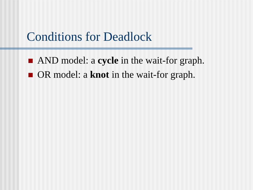
Conditions for Deadlock
AND model: a cycle in the wait-for graph.
OR model: a knot in the wait-for graph.

Conditions for Deadlock (Cont’d)
A knot (K) consists of a set of nodes such that for every node
a in K , all nodes in K and only the nodes in K are reachable
from node a.
Two systems under the OR condition with
(a) no deadlock and without (b) deadlock.

Focus 12: Rosenkrantz' Dynamic Priority
Scheme (using timestamps)
T1: lock A; lock B; transaction starts; unlock A; unlock B; wait-die (non-preemptive method) [ LCi < LCj halt Pi (wait) LCi LCj kill Pi (die) ] wound-wait (preemptive method) [ LCi < LCj kill Pj (wound) LCi LCj halt Pi (wait) ]
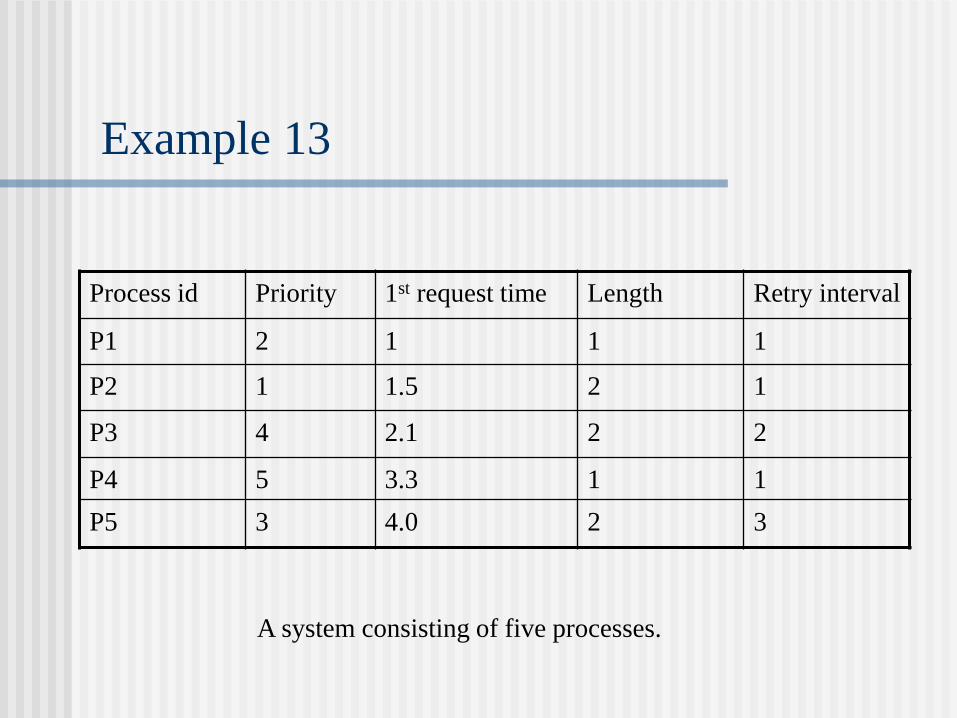
Example 13
A system consisting of five processes.
Process id Priority 1st request time Length Retry interval
P1 2 1 1 1
P2 1 1.5 2 1
P3 4 2.1 2 2
P4 5 3.3 1 1
P5 3 4.0 2 3
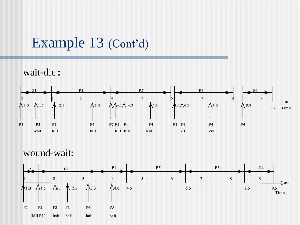
Example 13 (Cont’d)
wound-wait:
wait-die:
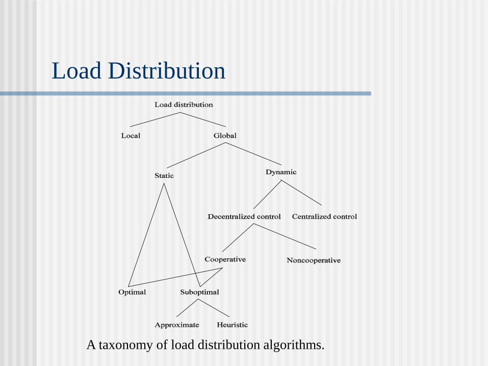
Load Distribution
A taxonomy of load distribution algorithms.
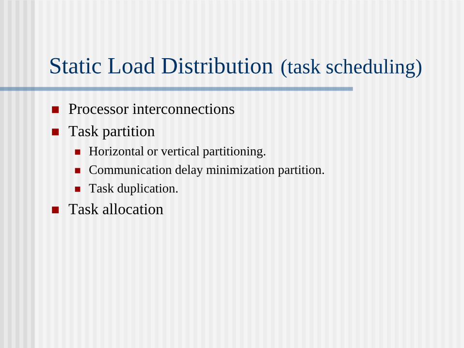
Static Load Distribution (task scheduling)
Processor interconnections
Task partition
Horizontal or vertical partitioning.
Communication delay minimization partition.
Task duplication.
Task allocation
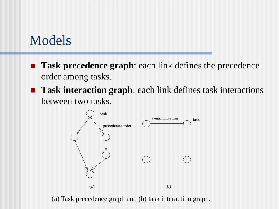
Models
Task precedence graph: each link defines the precedence
order among tasks.
Task interaction graph: each link defines task interactions
between two tasks.
(a) Task precedence graph and (b) task interaction graph.
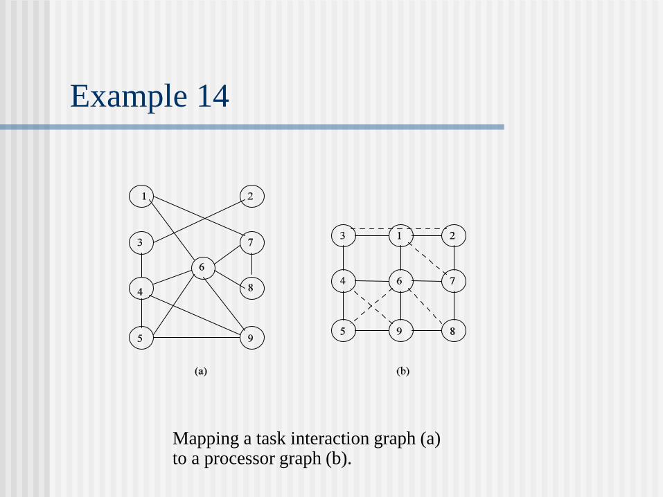
Example 14
Mapping a task interaction graph (a) to a processor graph (b).
Example 14 (Cont’d)
The dilation of an edge of Gt is defined as the length of the path in Gp onto which an edge of Gt is mapped. The dilation of the embedding is the maximum edge dilation of Gt.
The expansion of the embedding is the ratio of the number of nodes in Gt to the number of nodes in Gp.
The congestion of the embedding is the maximum number of paths containing an edge in Gp where every path represents an edge in Gt.
The load of an embedding is the maximum number of processes of Gt assigned to any processor of Gt.
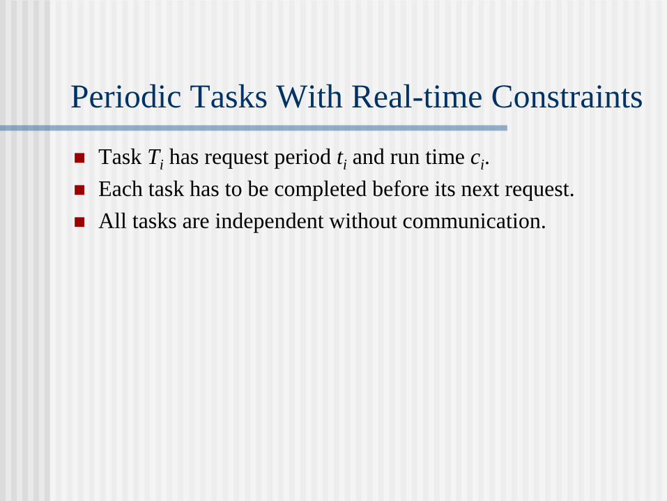
Periodic Tasks With Real-time Constraints
Task Ti has request period ti and run time ci.
Each task has to be completed before its next request.
All tasks are independent without communication.
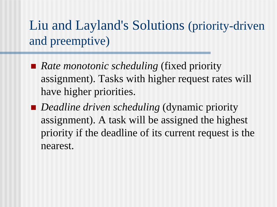
Liu and Layland's Solutions (priority-driven
and preemptive)
Rate monotonic scheduling (fixed priority
assignment). Tasks with higher request rates will
have higher priorities.
Deadline driven scheduling (dynamic priority
assignment). A task will be assigned the highest
priority if the deadline of its current request is the
nearest.
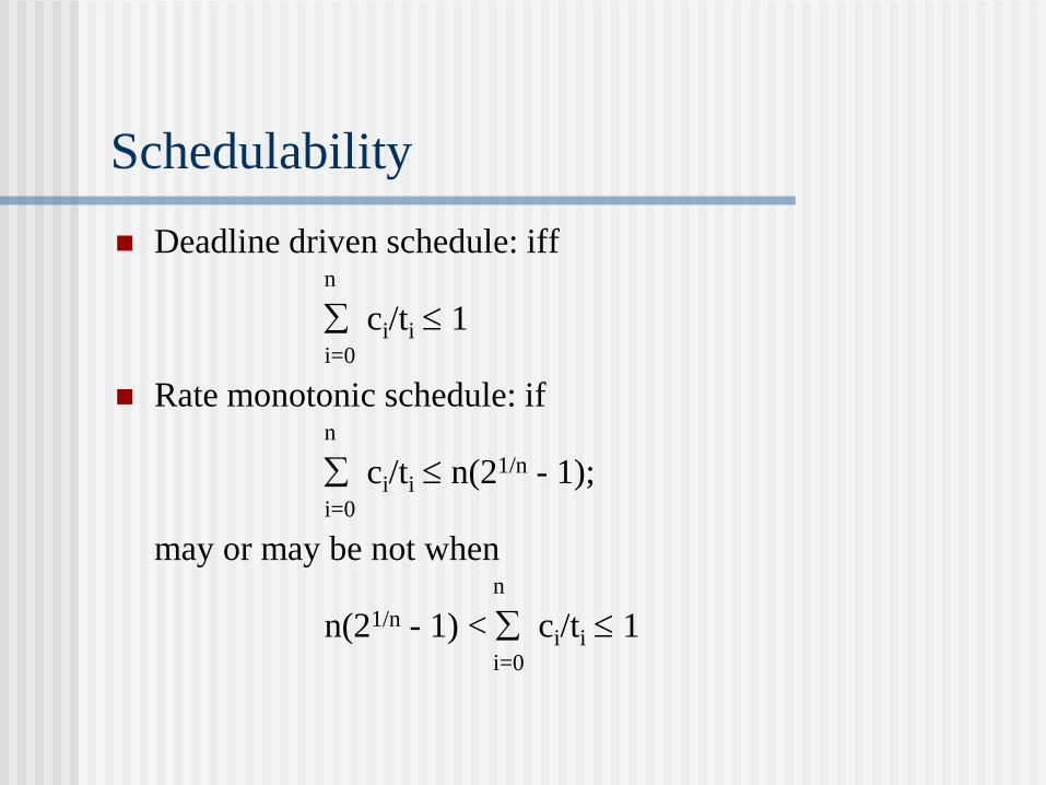
Schedulability
Deadline driven schedule: iff n
ci/ti 1 i=0
Rate monotonic schedule: if n
ci/ti n(21/n - 1); i=0
may or may be not when n
n(21/n - 1) < ci/ti 1 i=0

Example 15 (schedulable)
T1: c1 = 3, t1 = 5 and T2: c2 = 2, t2 = 7 (with the same initial
request time).
The overall utilization is 0:887 > 0:828 (bound for n = 2).
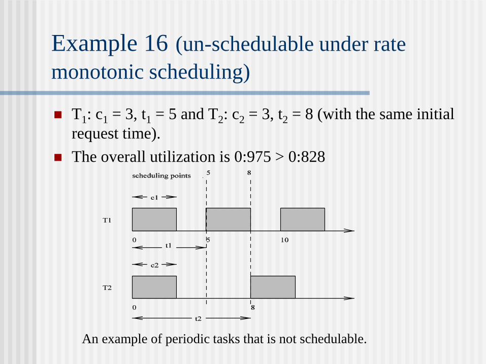
Example 16 (un-schedulable under rate
monotonic scheduling)
T1: c1 = 3, t1 = 5 and T2: c2 = 3, t2 = 8 (with the same initial
request time).
The overall utilization is 0:975 > 0:828
An example of periodic tasks that is not schedulable.

Example 16 (Cont’d)
If each task meets its first deadline when all tasks are started
at the same time then the deadlines for all tasks will always
be met for any combination of starting times.
scheduling points for task T : T 's first deadline and the ends
of periods of higher priority tasks prior to T 's first deadline.
If the task set is schedulable for one of scheduling points of
the lowest priority task, the task set is schedulable; otherwise,
the task set is not schedulable.
Example 17 (schedulable under rate
monotonic schedule)
c1 = 40, t1 = 100, c2 = 50, t2 = 150, and c3 = 80, t3 = 350.
The overall utilization is 0:2 + 0:333 + 0:229 = 0:762 < 0:779
(the bound for n > 3).
c1 is doubled to 40. The overall utilization is
0:4+0:333+0:229 = 0:962 > 0:779.
The scheduling points for T3: 350 (for T3), 300 (for T1 and
T2), 200 (for T1), 150 (for T2), 100 (for T1).
Example 17 (Cont’d)
c1 + c2 + c3 t1,
40 + 50 + 80 > 100;
2c1 + c2 + c3 t2,
80 + 50 + 80 > 150;
2c1 + 2c2 + c3 2t2,
80 + 100 + 80 > 200;
3c1 + 2c2 + c3 2t3,
120 + 100 + 80 = 300;
4c1 + 3c2 + c3 t1,
160 + 150 + 80 > 350.
Example 17 (Cont’d)
A schedulable periodic task.
Dynamic Load Distribution (load balancing)
A state-space traversal example.
Dynamic Load Distribution (Cont’d)
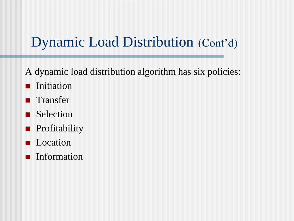
A dynamic load distribution algorithm has six policies:
Initiation
Transfer
Selection
Profitability
Location
Information
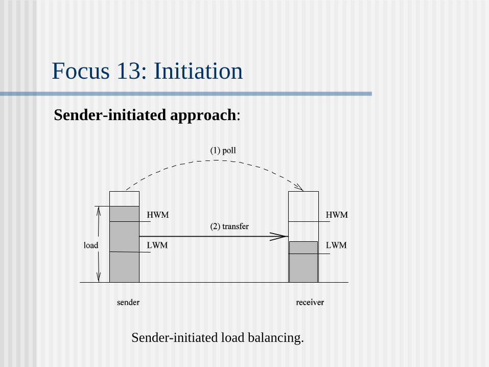
Focus 13: Initiation
Sender-initiated approach:
Sender-initiated load balancing.
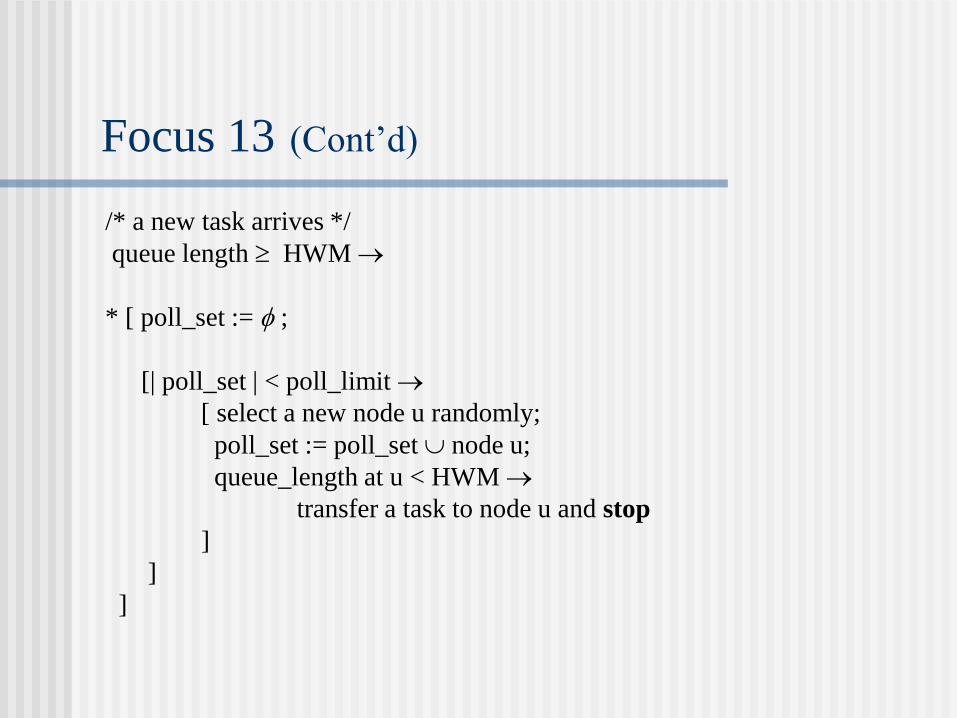
Focus 13 (Cont’d)
/* a new task arrives */
queue length HWM
* [ poll_set := ;
[| poll_set | < poll_limit
[ select a new node u randomly;
poll_set := poll_set node u;
queue_length at u < HWM
transfer a task to node u and stop
]
]
]
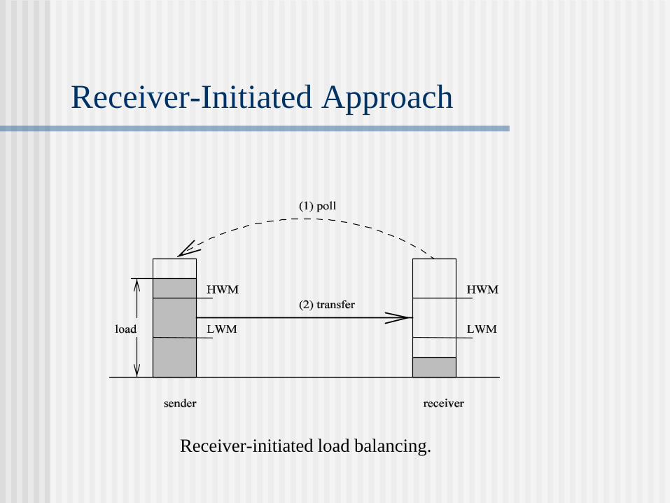
Receiver-Initiated Approach
Receiver-initiated load balancing.

Receiver-Initiated Approach (Cont’d)
/* a task departs */
queue length < LWM
[ poll limit:= ;
* [ | poll_set | < poll limit
[ select a new node u randomly;
poll_set := poll set node u;
queue_length at u > HWM
transfer a task from node u and stop
]
]
]

Bidding Approach
Bidding algorithm.
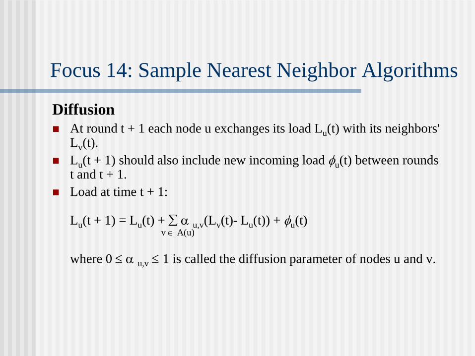
Focus 14: Sample Nearest Neighbor Algorithms
Diffusion
At round t + 1 each node u exchanges its load Lu(t) with its neighbors' Lv(t).
Lu(t + 1) should also include new incoming load u(t) between rounds t and t + 1.
Load at time t + 1: Lu(t + 1) = Lu(t) + u,v(Lv(t)- Lu(t)) + u(t) v A(u)
where 0 u,v 1 is called the diffusion parameter of nodes u and v.
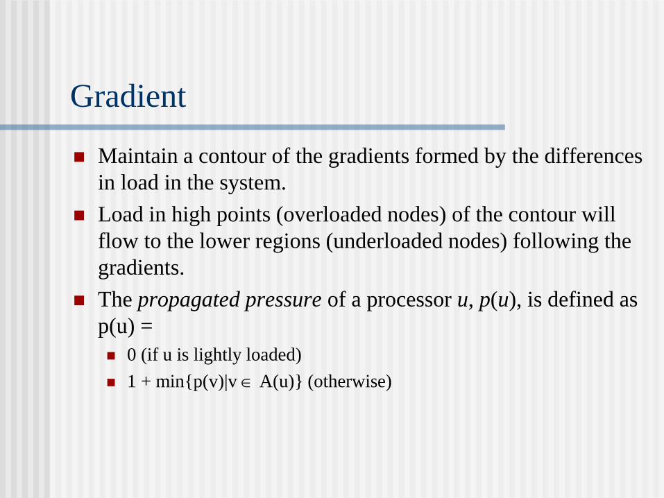
Gradient
Maintain a contour of the gradients formed by the differences
in load in the system.
Load in high points (overloaded nodes) of the contour will
flow to the lower regions (underloaded nodes) following the
gradients.
The propagated pressure of a processor u, p(u), is defined as
p(u) =
0 (if u is lightly loaded)
1 + min{p(v)|v A(u)} (otherwise)

Gradient (Cont’d)
(a) A 4 x 4 mesh with loads. (b) The corresponding propagated
pressure of each node (a node is lightly loaded if its load is less than 3).
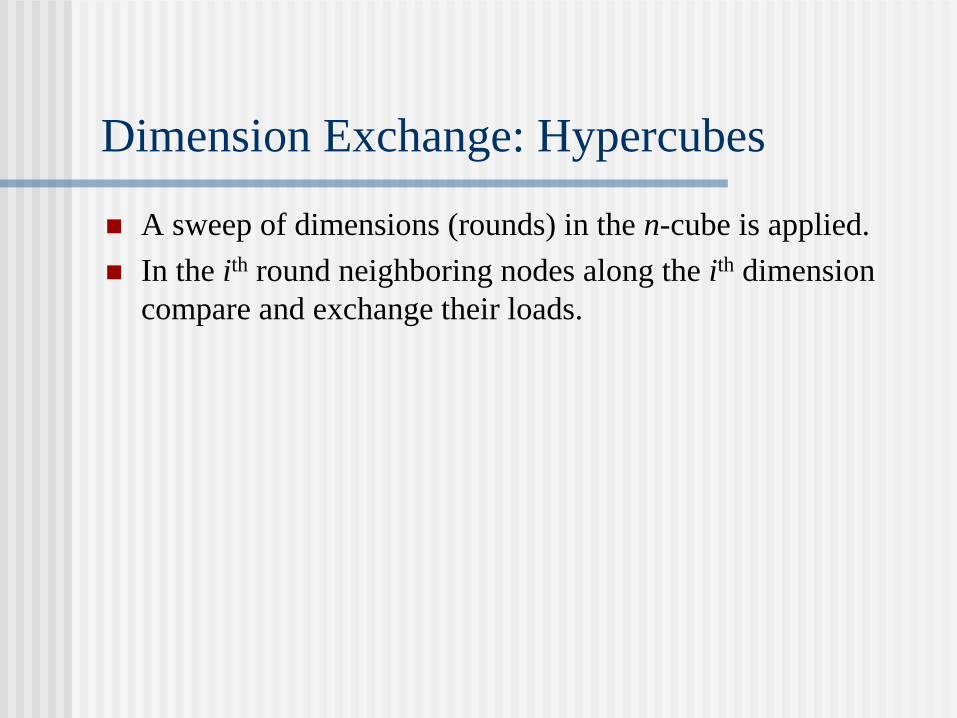
Dimension Exchange: Hypercubes
A sweep of dimensions (rounds) in the n-cube is applied.
In the ith round neighboring nodes along the ith dimension
compare and exchange their loads.
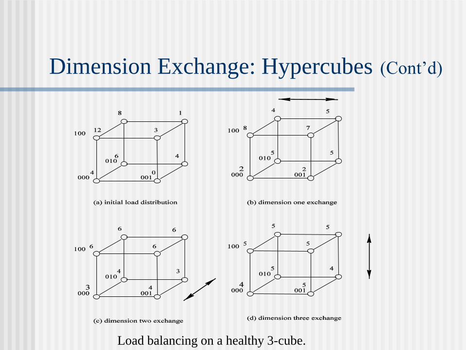
Dimension Exchange: Hypercubes (Cont’d)
Load balancing on a healthy 3-cube.
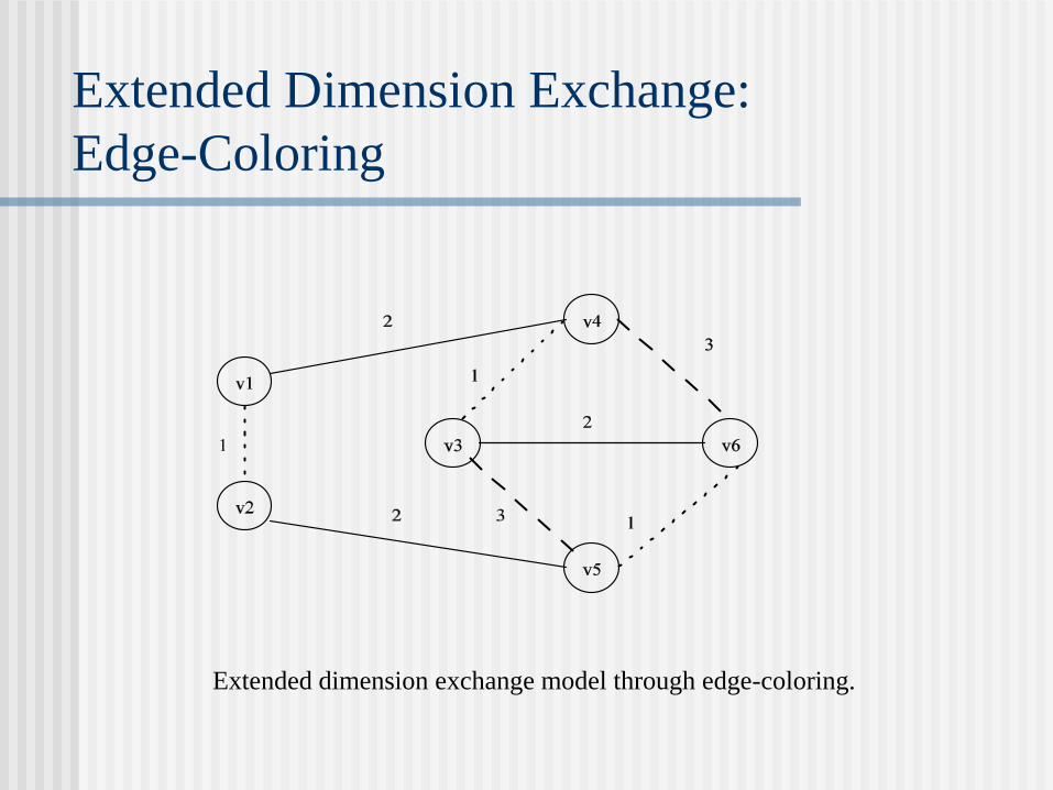
Extended Dimension Exchange:
Edge-Coloring
Extended dimension exchange model through edge-coloring.
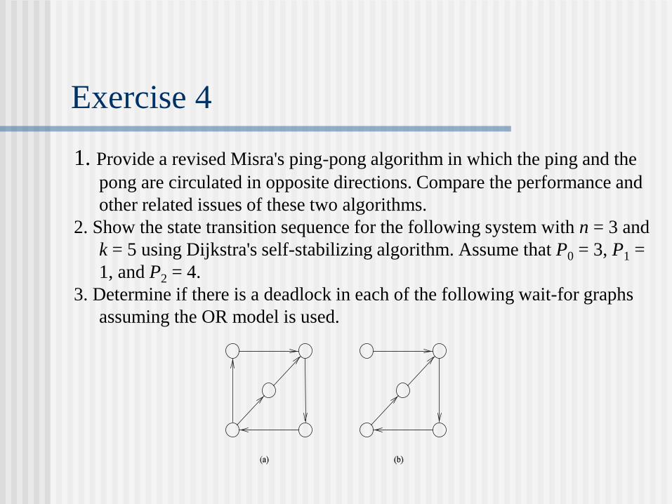
Exercise 4
1. Provide a revised Misra's ping-pong algorithm in which the ping and the
pong are circulated in opposite directions. Compare the performance and
other related issues of these two algorithms.
2. Show the state transition sequence for the following system with n = 3 and
k = 5 using Dijkstra's self-stabilizing algorithm. Assume that P0 = 3, P1 =
1, and P2 = 4.
3. Determine if there is a deadlock in each of the following wait-for graphs
assuming the OR model is used.
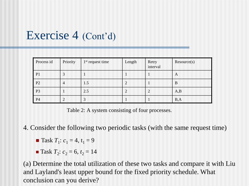
Exercise 4 (Cont’d)
Table 2: A system consisting of four processes.
Process id Priority 1st request time Length Retry
interval
Resource(s)
P1 3 1 1 1 A
P2 4 1.5 2 1 B
P3 1 2.5 2 2 A,B
P4 2 3 1 1 B,A
4. Consider the following two periodic tasks (with the same request time)
Task T1: c1 = 4, t1 = 9
Task T2: c2 = 6, t2 = 14
(a) Determine the total utilization of these two tasks and compare it with Liu
and Layland's least upper bound for the fixed priority schedule. What
conclusion can you derive?

Exercise 4 (Cont’d)
(b) Show that these two tasks are schedulable using the rate-monotonic
priority assignment. You are required to provide such a schedule.
(c) Determine the schedulability of these two tasks if task T2 has a higher
priority than task T1 in the fixed priority schedule.
(d) Split task T2 into two parts of 3 units computation each and show that
these two tasks are schedulable using the rate-monotonic priority
assignment.
(e) Provide a schedule (from time unit 0 to time unit 30) based on deadline
driven scheduling algorithm. Assume that the smallest preemptive
element is one unit.
Exercise 4 (Cont’d)
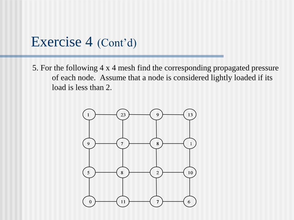
5. For the following 4 x 4 mesh find the corresponding propagated pressure
of each node. Assume that a node is considered lightly loaded if its
load is less than 2.
Table of Contents
Introduction and Motivation
Theoretical Foundations
Distributed Programming Languages
Distributed Operating Systems
Distributed Communication
Distributed Data Management
Reliability
Applications
Conclusions
Appendix

Distributed Communication
One-to-all (broadcast)
Different types of communication
One-to-one (unicast)
One-to-many (multicast)
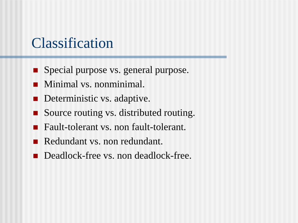
Classification
Special purpose vs. general purpose.
Minimal vs. nonminimal.
Deterministic vs. adaptive.
Source routing vs. distributed routing.
Fault-tolerant vs. non fault-tolerant.
Redundant vs. non redundant.
Deadlock-free vs. non deadlock-free.
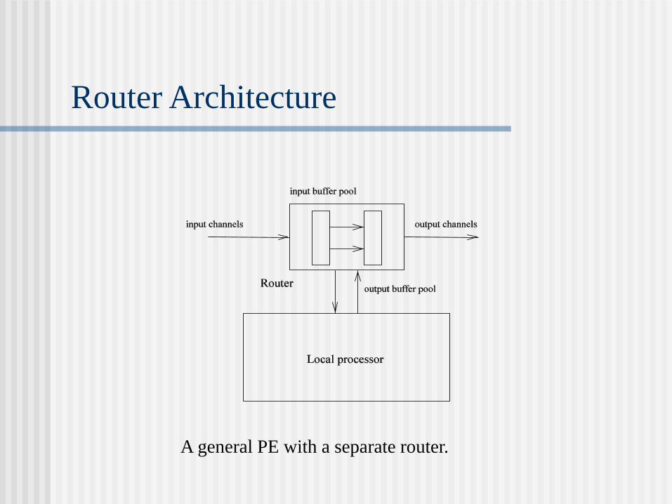
A general PE with a separate router.
Router Architecture
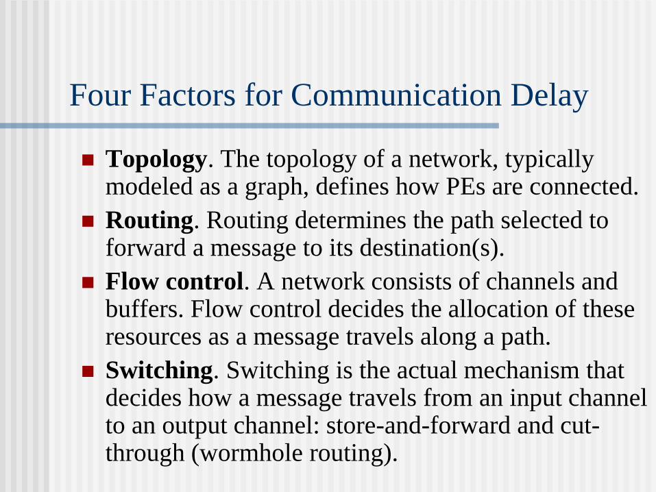
Topology. The topology of a network, typically modeled as a graph, defines how PEs are connected.
Routing. Routing determines the path selected to forward a message to its destination(s).
Flow control. A network consists of channels and buffers. Flow control decides the allocation of these resources as a message travels along a path.
Switching. Switching is the actual mechanism that decides how a message travels from an input channel to an output channel: store-and-forward and cut-through (wormhole routing).
Four Factors for Communication Delay

General-Purpose Routing
Source routing: link state (Dijkstra's algorithm)
A sample source routing
General-Purpose Routing (Cont’d)
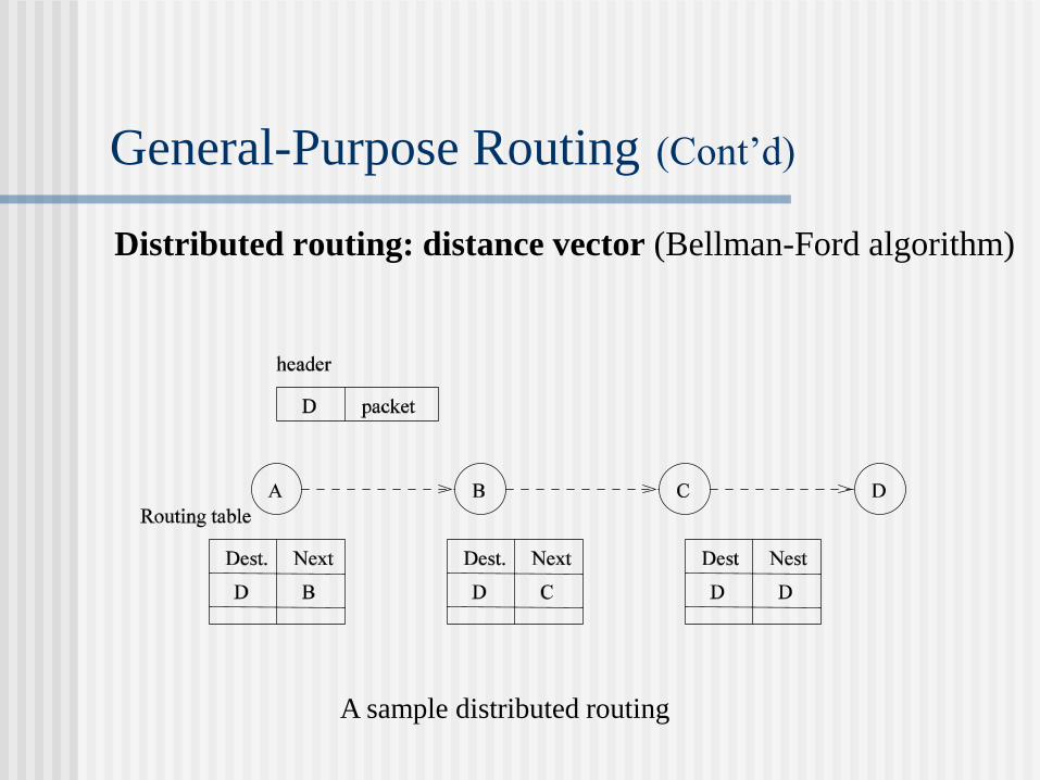
Distributed routing: distance vector (Bellman-Ford algorithm)
A sample distributed routing
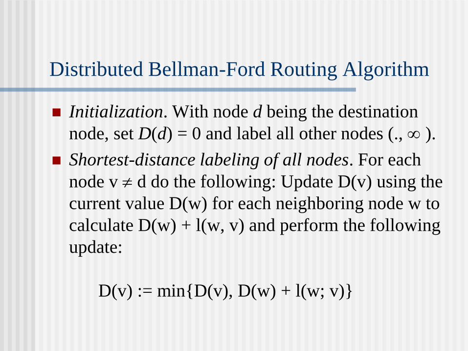
Distributed Bellman-Ford Routing Algorithm
Initialization. With node d being the destination
node, set D(d) = 0 and label all other nodes (., ).
Shortest-distance labeling of all nodes. For each
node v d do the following: Update D(v) using the
current value D(w) for each neighboring node w to
calculate D(w) + l(w, v) and perform the following
update:
D(v) := min{D(v), D(w) + l(w; v)}
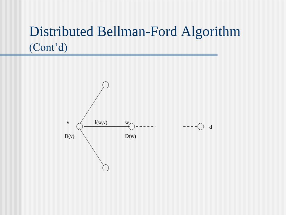
Distributed Bellman-Ford Algorithm (Cont’d)
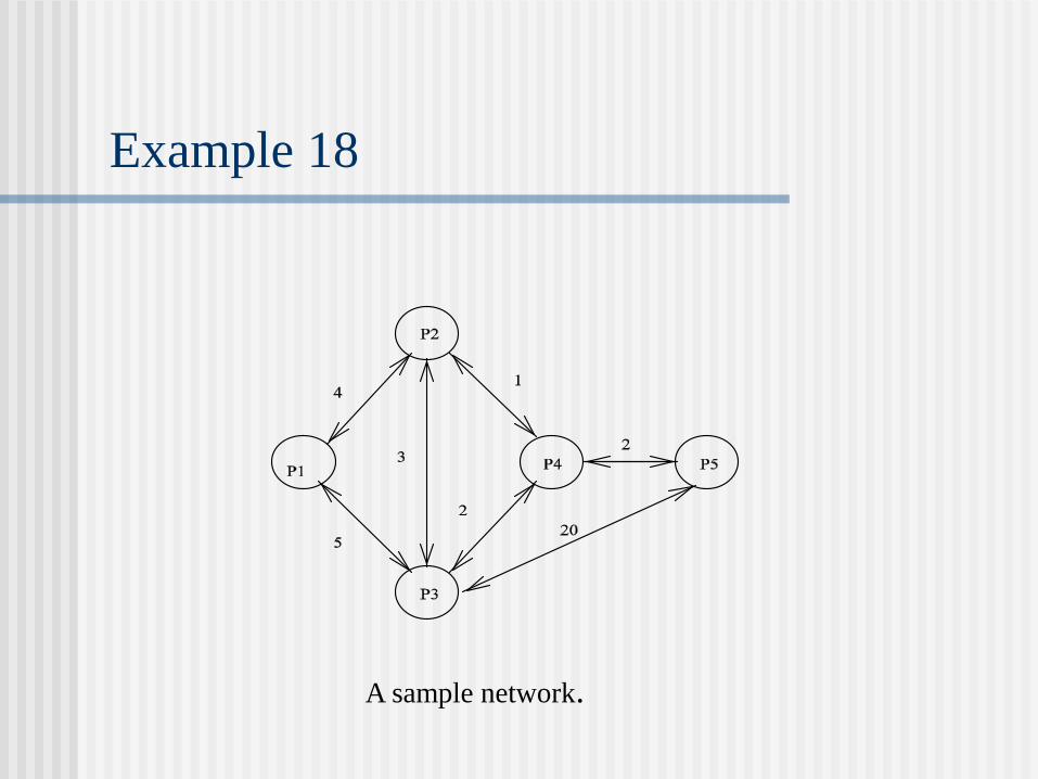
Example 18
A sample network.
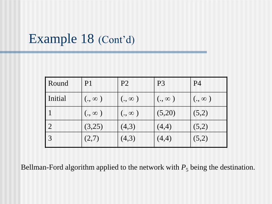
Example 18 (Cont’d)
Bellman-Ford algorithm applied to the network with P5 being the destination.
Round P1 P2 P3 P4
Initial (., ) (., ) (., ) (., )
1 (., ) (., ) (5,20) (5,2)
2 (3,25) (4,3) (4,4) (5,2)
3 (2,7) (4,3) (4,4) (5,2)
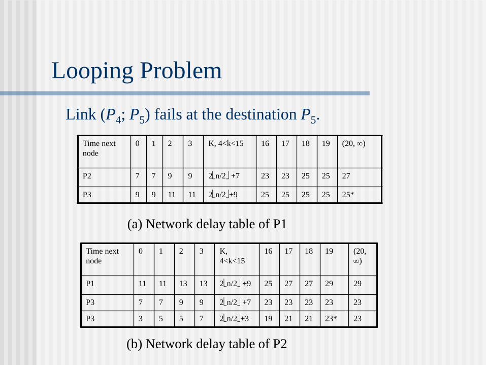
Looping Problem
Time next
node
0 1 2 3 K, 4<k<15 16 17 18 19 (20, )
P2 7 7 9 9 2n/2 +7 23 23 25 25 27
P3 9 9 11 11 2n/2+9 25 25 25 25 25*
Time next
node
0 1 2 3 K,
4<k<15
16 17 18 19 (20,
)
P1 11 11 13 13 2n/2 +9 25 27 27 29 29
P3 7 7 9 9 2n/2 +7 23 23 23 23 23
P3 3 5 5 7 2n/2+3 19 21 21 23* 23
(a) Network delay table of P1
(b) Network delay table of P2
Link (P4; P5) fails at the destination P5.
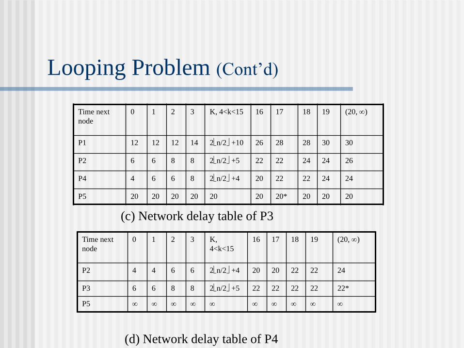
Time next
node
0 1 2 3 K, 4<k<15 16 17 18 19 (20, )
P1 12 12 12 14 2n/2 +10 26 28 28 30 30
P2 6 6 8 8 2n/2 +5 22 22 24 24 26
P4 4 6 6 8 2n/2 +4 20 22 22 24 24
P5 20 20 20 20 20 20 20* 20 20 20
Time next
node
0 1 2 3 K,
4<k<15
16 17 18 19 (20, )
P2 4 4 6 6 2n/2 +4 20 20 22 22 24
P3 6 6 8 8 2n/2 +5 22 22 22 22 22*
P5
(c) Network delay table of P3
(d) Network delay table of P4
Looping Problem (Cont’d)
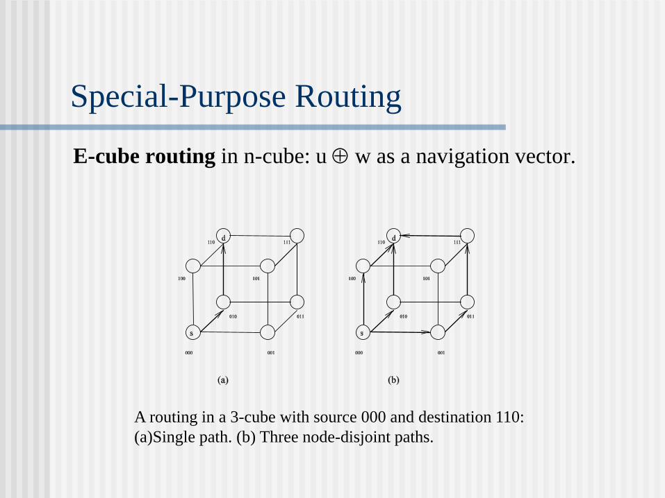
Special-Purpose Routing
E-cube routing in n-cube: u w as a navigation vector.
A routing in a 3-cube with source 000 and destination 110:
(a)Single path. (b) Three node-disjoint paths.
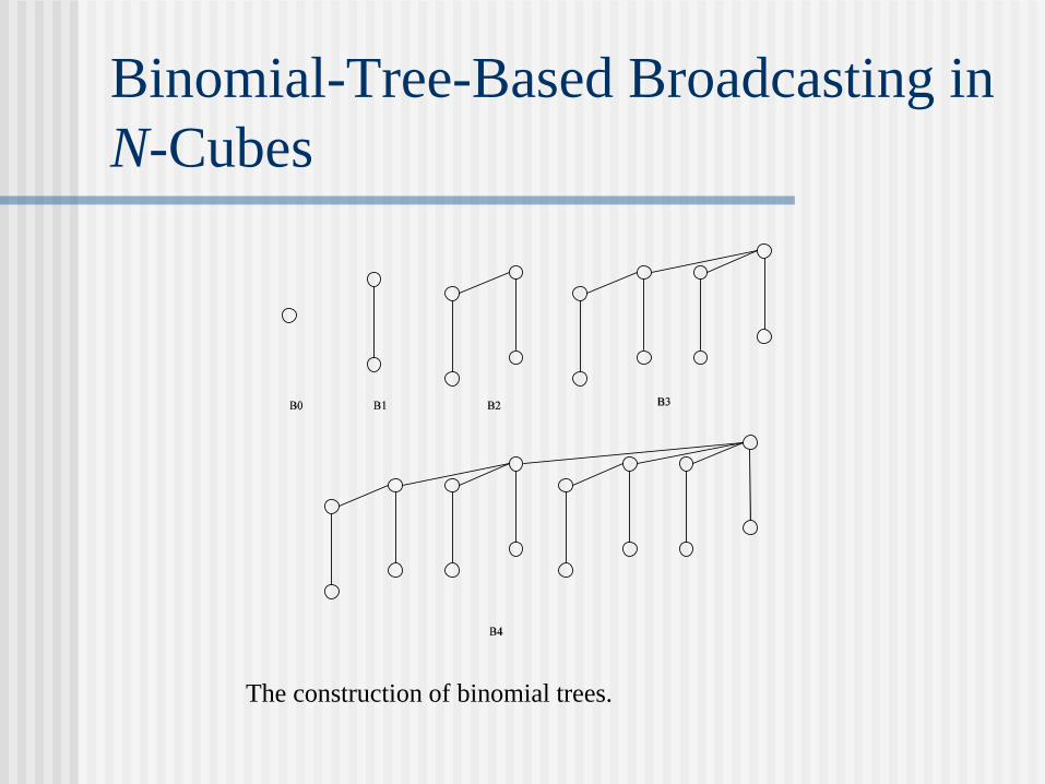
Binomial-Tree-Based Broadcasting in
N-Cubes
The construction of binomial trees.
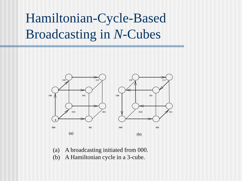
Hamiltonian-Cycle-Based
Broadcasting in N-Cubes
(a) A broadcasting initiated from 000.
(b) A Hamiltonian cycle in a 3-cube.
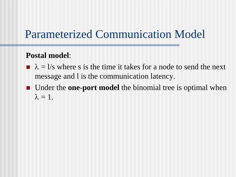
Parameterized Communication Model
Postal model:
= l/s where s is the time it takes for a node to send the next
message and l is the communication latency.
Under the one-port model the binomial tree is optimal when
= 1.
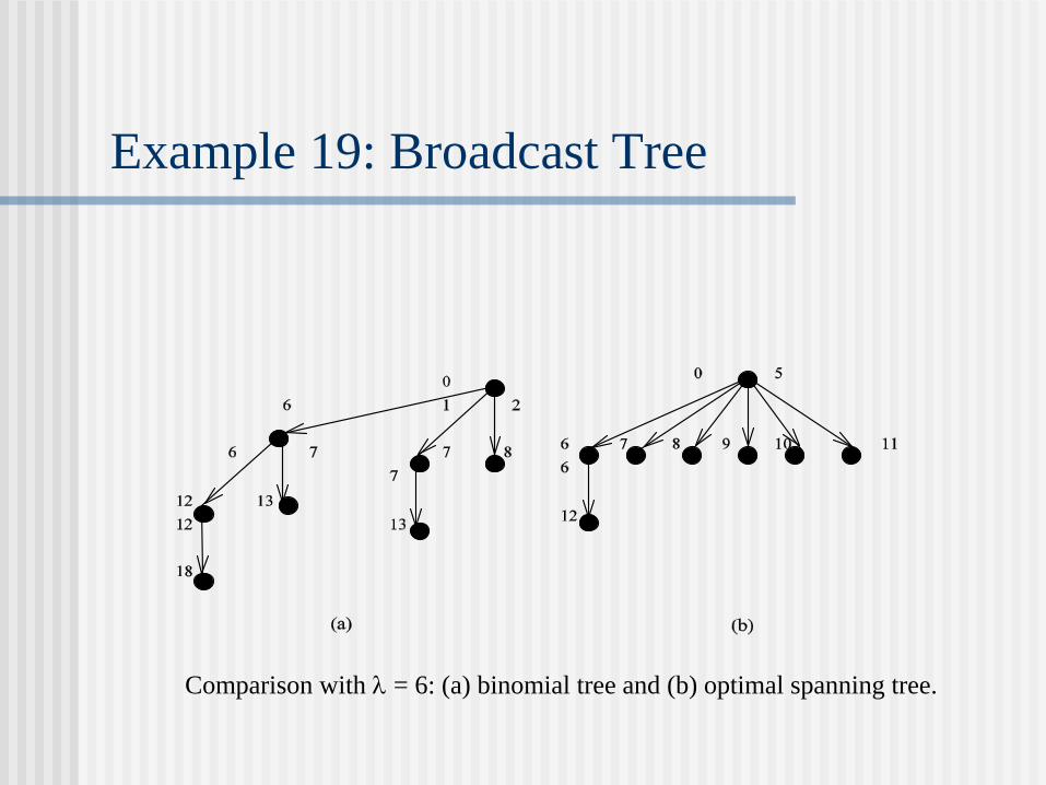
Example 19: Broadcast Tree
Comparison with = 6: (a) binomial tree and (b) optimal spanning tree.
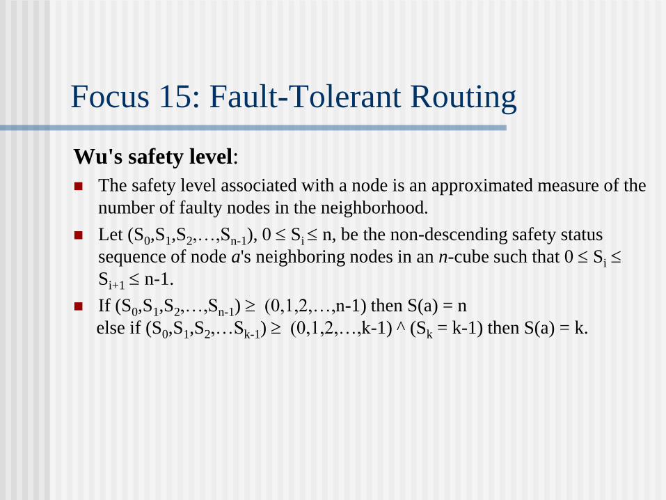
Focus 15: Fault-Tolerant Routing
Wu's safety level:
The safety level associated with a node is an approximated measure of the
number of faulty nodes in the neighborhood.
Let (S0,S1,S2,…,Sn-1), 0 Si n, be the non-descending safety status
sequence of node a's neighboring nodes in an n-cube such that 0 Si
Si+1 n-1.
If (S0,S1,S2,…,Sn-1) (0,1,2,…,n-1) then S(a) = n
else if (S0,S1,S2,…Sk-1) (0,1,2,…,k-1) ^ (Sk = k-1) then S(a) = k.
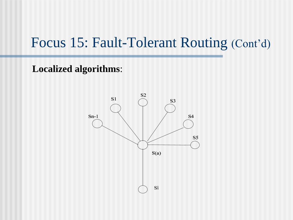
Focus 15: Fault-Tolerant Routing (Cont’d)
Localized algorithms:
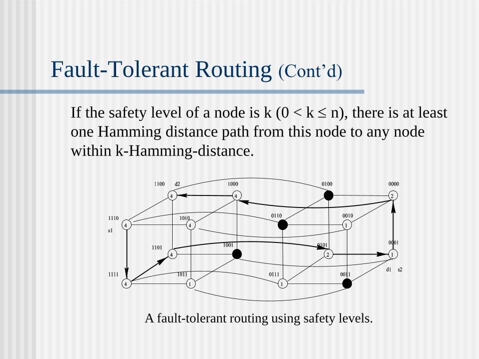
Fault-Tolerant Routing (Cont’d)
If the safety level of a node is k (0 < k n), there is at least
one Hamming distance path from this node to any node
within k-Hamming-distance.
A fault-tolerant routing using safety levels.
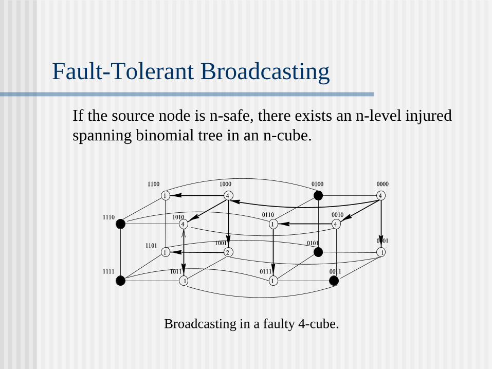
Fault-Tolerant Broadcasting
If the source node is n-safe, there exists an n-level injured
spanning binomial tree in an n-cube.
Broadcasting in a faulty 4-cube.
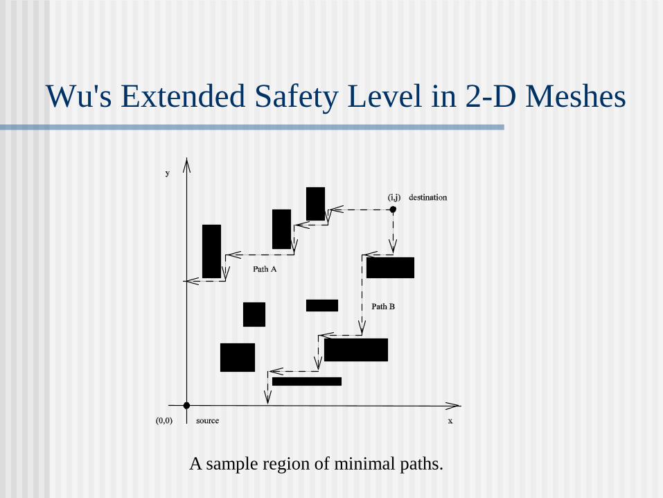
Wu's Extended Safety Level in 2-D Meshes
A sample region of minimal paths.
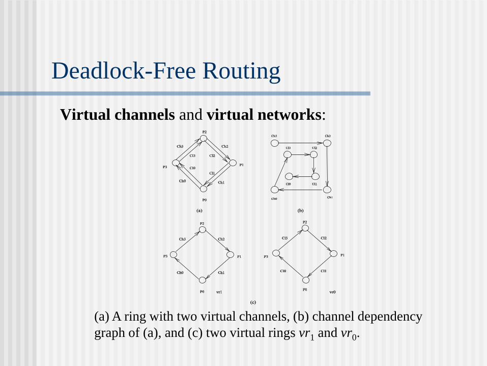
Deadlock-Free Routing
Virtual channels and virtual networks:
(a) A ring with two virtual channels, (b) channel dependency
graph of (a), and (c) two virtual rings vr1 and vr0.
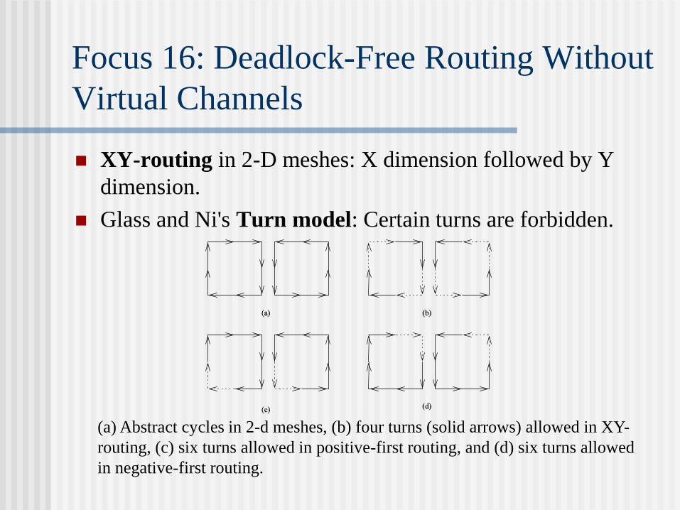
Focus 16: Deadlock-Free Routing Without
Virtual Channels
XY-routing in 2-D meshes: X dimension followed by Y
dimension.
Glass and Ni's Turn model: Certain turns are forbidden.
(a) Abstract cycles in 2-d meshes, (b) four turns (solid arrows) allowed in XY-
routing, (c) six turns allowed in positive-first routing, and (d) six turns allowed
in negative-first routing.

Basic Routing Strategies in Internet
Source routing: link state
Distributed routing: distance vector
Figure 1: A sample source routing
Figure 2: A sample distributed routing

Routing in Ad Hoc Wireless Networks
The dynamic nature of ad hoc wireless networks
presents a challenge to current routing techniques.

Major Challenges
Scalable design
Low power design
Mobility management
Low latency
Classification
Proactive vs. reactive
proactive: continuously evaluate network connectivity
reactive: invoke a route determination procedure on-
demand.
Flat vs. cluster-based
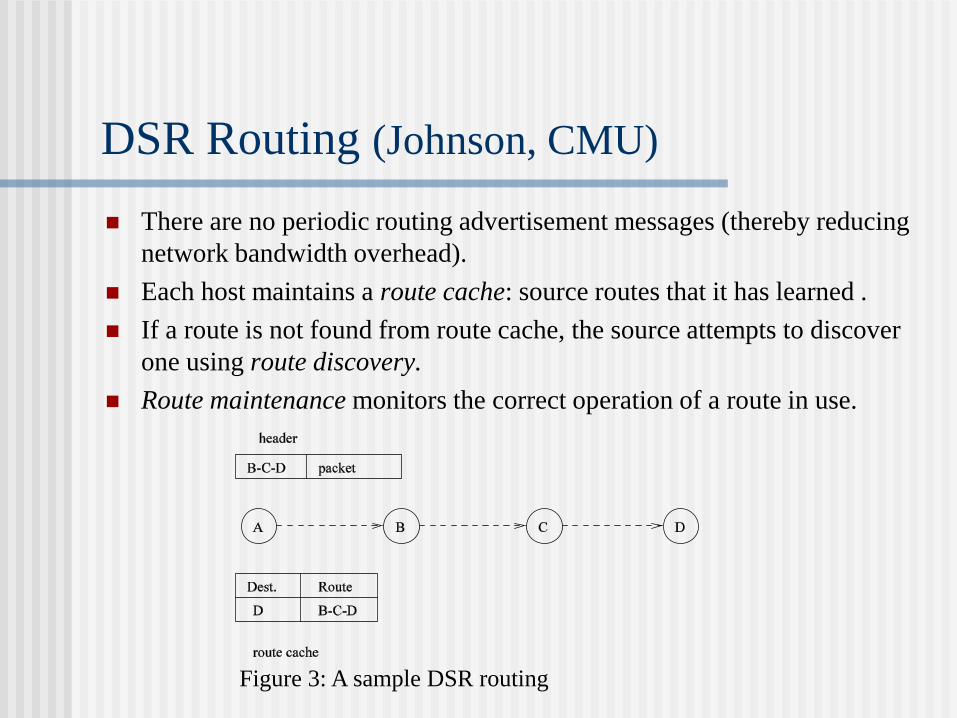
DSR Routing (Johnson, CMU)
There are no periodic routing advertisement messages (thereby reducing
network bandwidth overhead).
Each host maintains a route cache: source routes that it has learned .
If a route is not found from route cache, the source attempts to discover
one using route discovery.
Route maintenance monitors the correct operation of a route in use.
Figure 3: A sample DSR routing
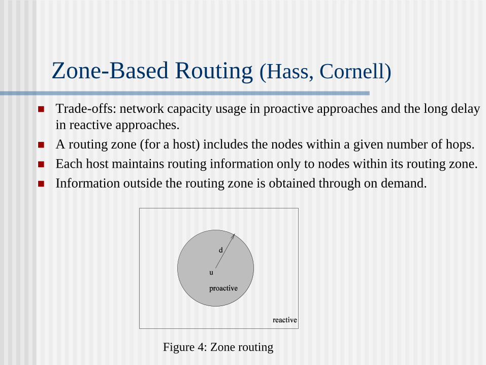
Zone-Based Routing (Hass, Cornell)
Trade-offs: network capacity usage in proactive approaches and the long delay
in reactive approaches.
A routing zone (for a host) includes the nodes within a given number of hops.
Each host maintains routing information only to nodes within its routing zone.
Information outside the routing zone is obtained through on demand.
Figure 4: Zone routing
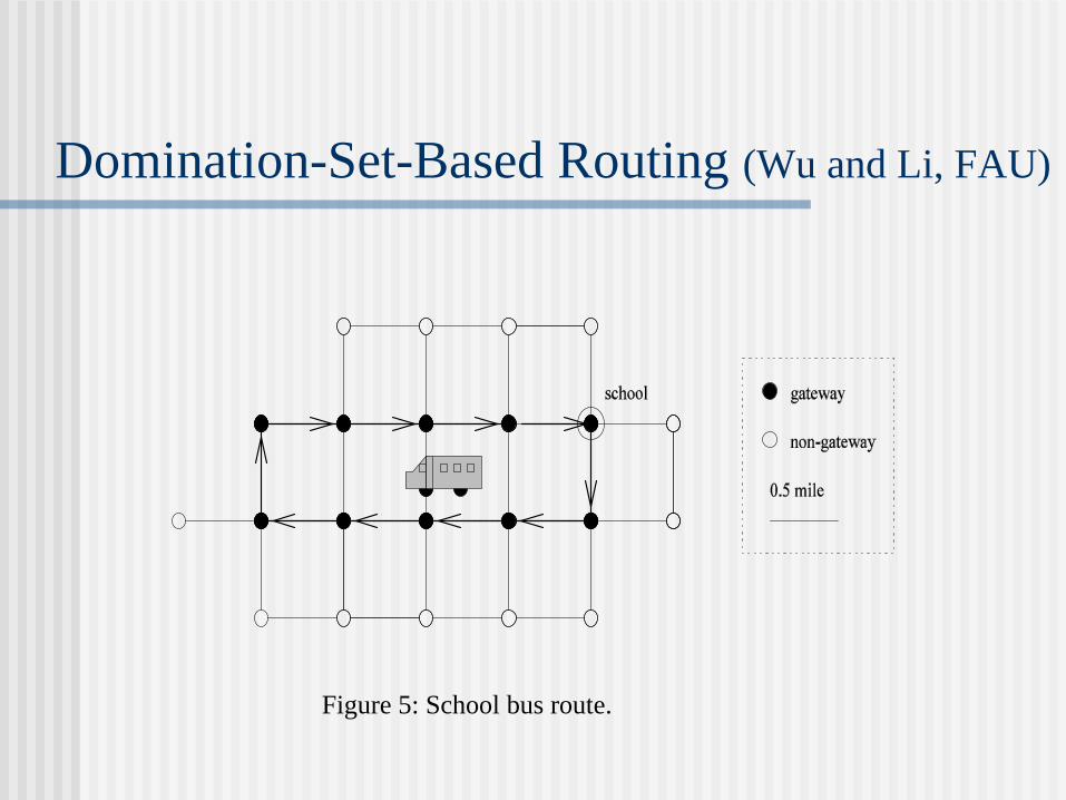
Domination-Set-Based Routing (Wu and Li, FAU)
Figure 5: School bus route.
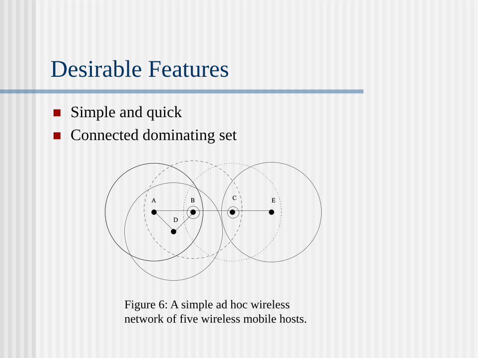
Desirable Features
Simple and quick
Connected dominating set
Figure 6: A simple ad hoc wireless
network of five wireless mobile hosts.

Existing Approaches
Graph theory community:
Bounds on the domination number (Haynes, Hedetniemi, and Slater,
1998).
Special classes of graph for which the domination problem can be
solved in polynomial time.
Ad hoc wireless network community:
Global: MCDS (Sivakumar, Das, and Bharghavan, 1998).
Quasi-global: spanning-tree-based (Wan, Alzoubi, and Frieder,
2002).
Quasi-local: cluster-based (Lin and Gerla, 1999).
Local: marking process (Wu and Li, 1999).
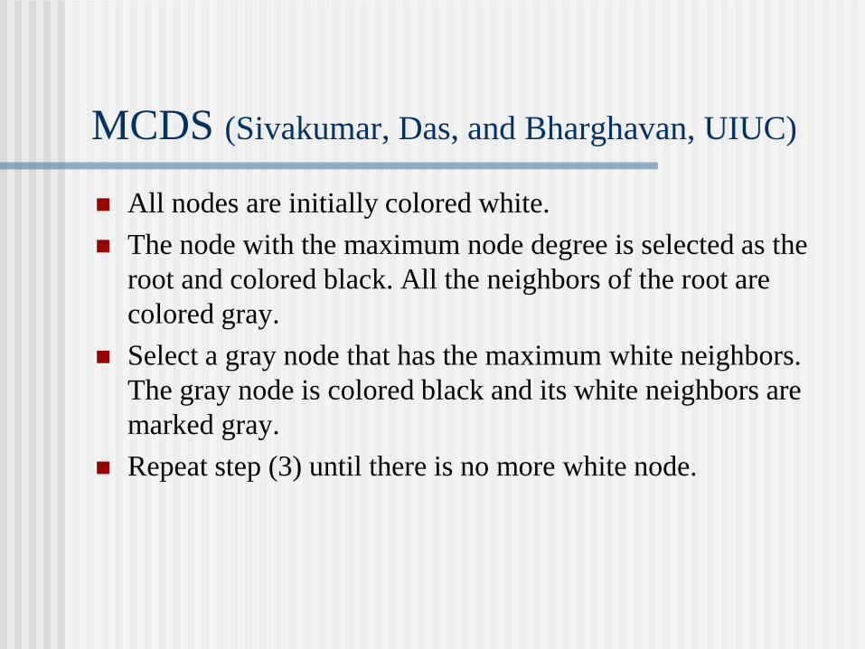
MCDS (Sivakumar, Das, and Bharghavan, UIUC)
All nodes are initially colored white.
The node with the maximum node degree is selected as the
root and colored black. All the neighbors of the root are
colored gray.
Select a gray node that has the maximum white neighbors.
The gray node is colored black and its white neighbors are
marked gray.
Repeat step (3) until there is no more white node.
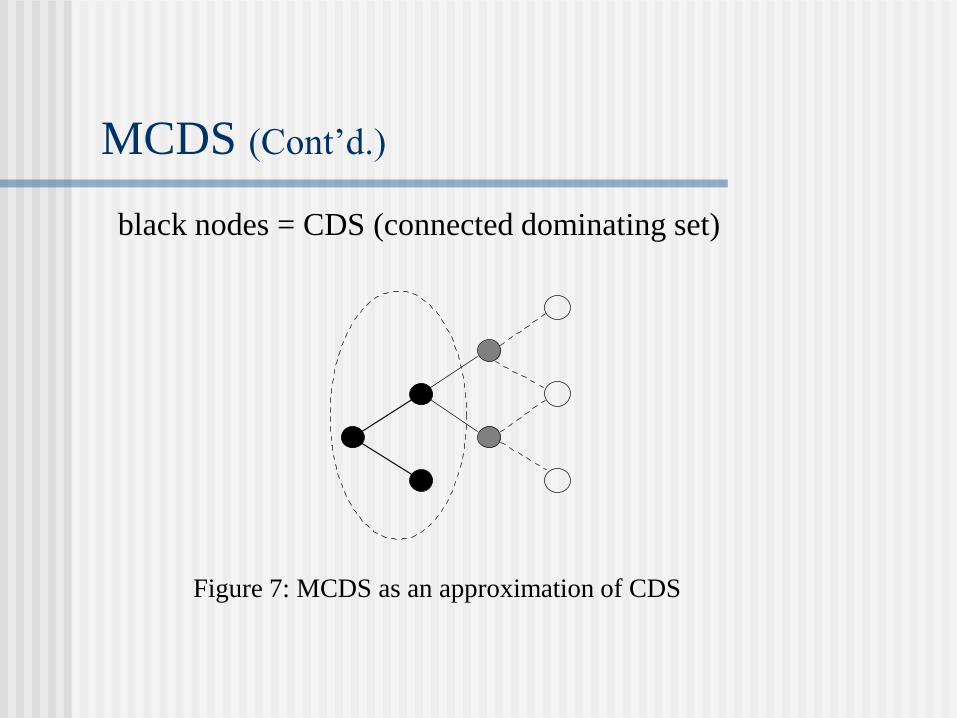
MCDS (Cont’d.)
black nodes = CDS (connected dominating set)
Figure 7: MCDS as an approximation of CDS
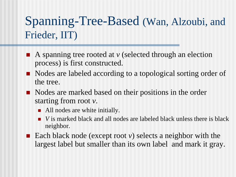
Spanning-Tree-Based (Wan, Alzoubi, and
Frieder, IIT)
A spanning tree rooted at v (selected through an election process) is first constructed.
Nodes are labeled according to a topological sorting order of the tree.
Nodes are marked based on their positions in the order starting from root v.
All nodes are white initially.
V is marked black and all nodes are labeled black unless there is black neighbor.
Each black node (except root v) selects a neighbor with the largest label but smaller than its own label and mark it gray.
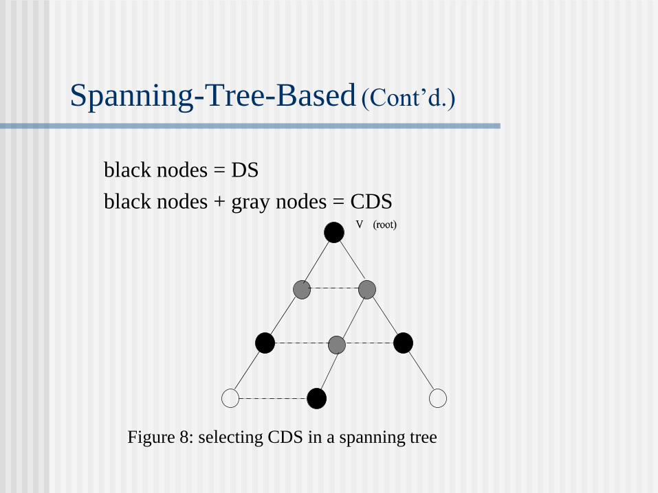
Spanning-Tree-Based (Cont’d.)
black nodes = DS
black nodes + gray nodes = CDS
Figure 8: selecting CDS in a spanning tree

Cluster-Based (Lee and Gerla, UCLA)
All nodes are initially white.
When a white node finds itself having the lowest id among all
its white neighbors, it becomes a cluster head and colors itself
black.
All its neighbors join in the cluster and change their colors to
gray.
Repeat steps (1) and (2) until there is no white node left.
Special gray nodes: gray nodes that have two neighbors in
different clusters.
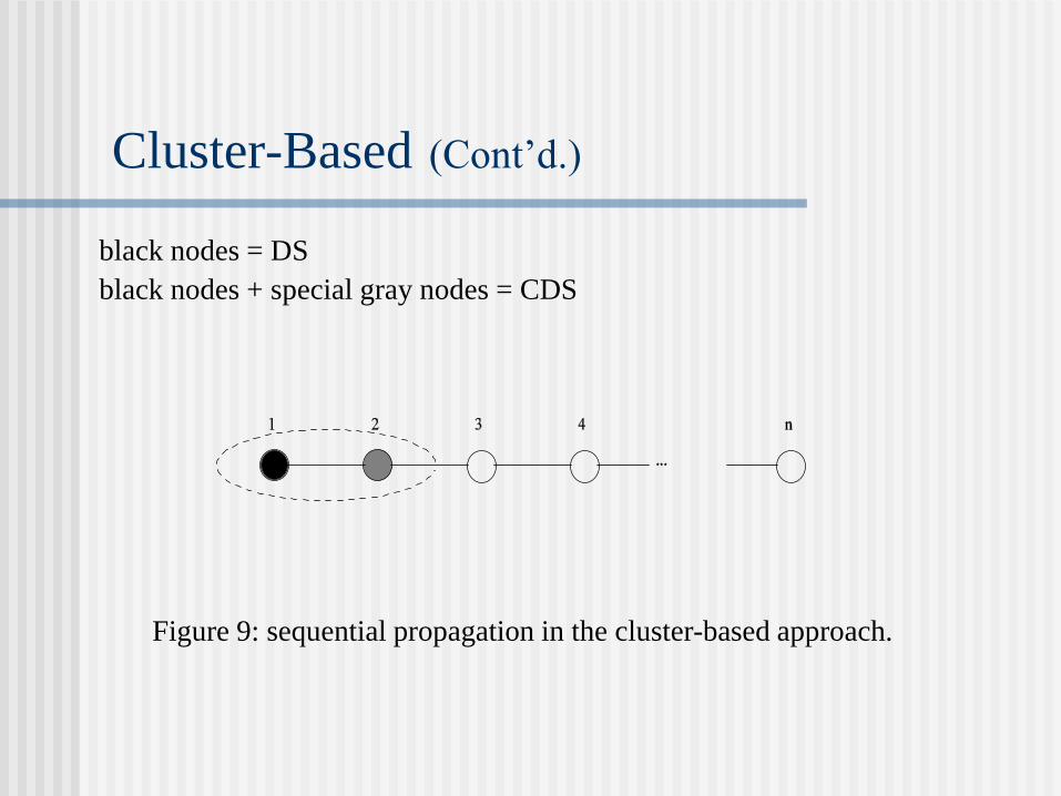
Cluster-Based (Cont’d.)
black nodes = DS
black nodes + special gray nodes = CDS
Figure 9: sequential propagation in the cluster-based approach.
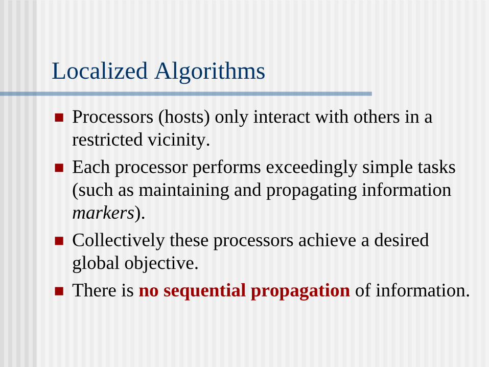
Localized Algorithms
Processors (hosts) only interact with others in a
restricted vicinity.
Each processor performs exceedingly simple tasks
(such as maintaining and propagating information
markers).
Collectively these processors achieve a desired
global objective.
There is no sequential propagation of information.
Focus 17: Wu and Li's Marking Process
A node is marked true if it has two unconnected
neighbors.
A set of marked nodes (gateways nodes) V’ form a
connected dominating set.

Example 20
Figure 10: A sample ad hoc wireless network
Properties
Property 1: V’ is empty if and only if G is a complete graph;
otherwise, V’ forms a dominating set.
Property 2: V’ includes all the intermediate vertices of any
shortest path.
Property 3: The induced graph G’ = G[V’] is a connected
graph.
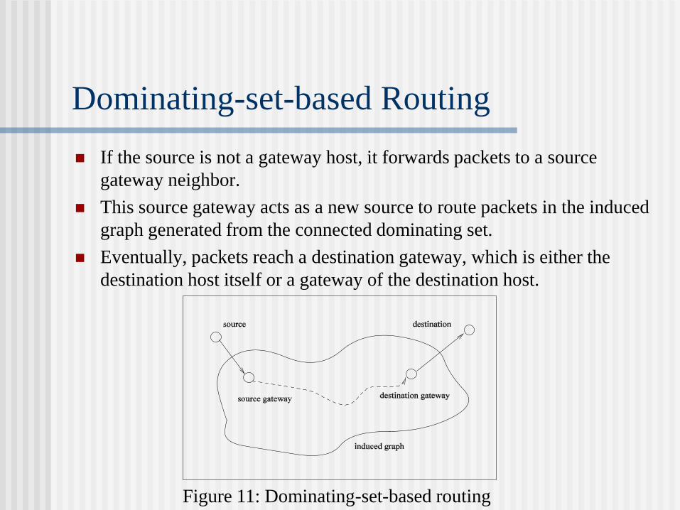
Dominating-set-based Routing
If the source is not a gateway host, it forwards packets to a source
gateway neighbor.
This source gateway acts as a new source to route packets in the induced
graph generated from the connected dominating set.
Eventually, packets reach a destination gateway, which is either the
destination host itself or a gateway of the destination host.
Figure 11: Dominating-set-based routing
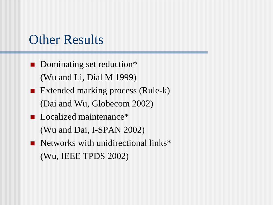
Other Results
Dominating set reduction*
(Wu and Li, Dial M 1999)
Extended marking process (Rule-k)
(Dai and Wu, Globecom 2002)
Localized maintenance*
(Wu and Dai, I-SPAN 2002)
Networks with unidirectional links*
(Wu, IEEE TPDS 2002)
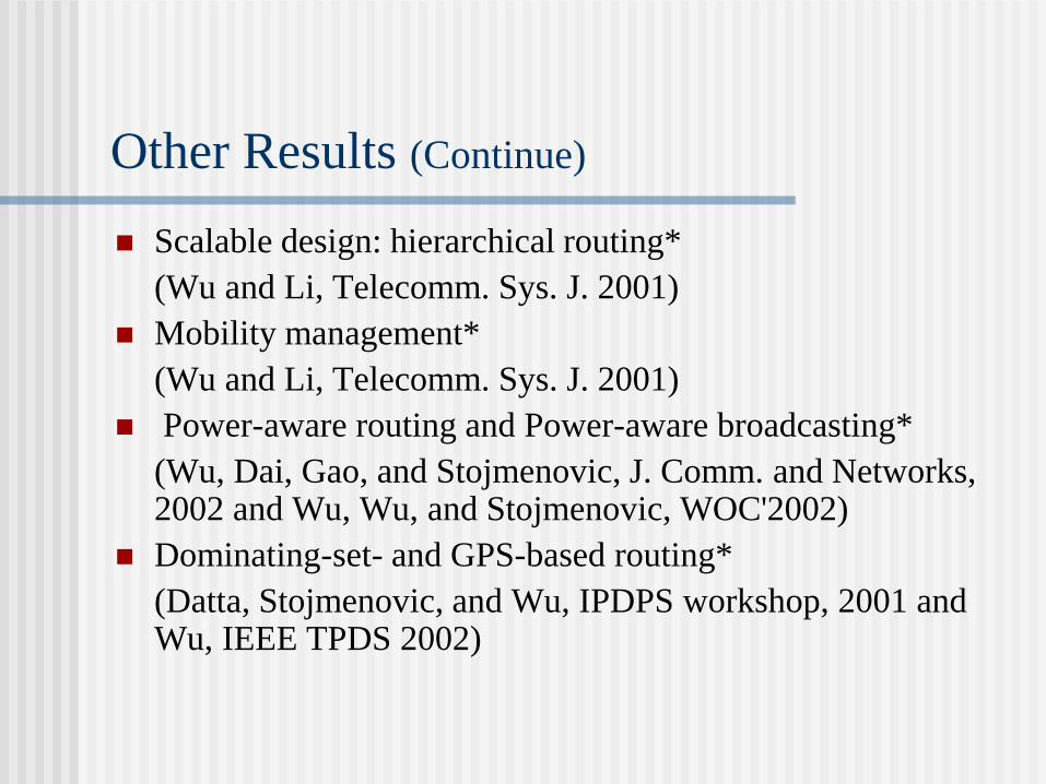
Other Results (Continue)
Scalable design: hierarchical routing*
(Wu and Li, Telecomm. Sys. J. 2001)
Mobility management*
(Wu and Li, Telecomm. Sys. J. 2001)
Power-aware routing and Power-aware broadcasting*
(Wu, Dai, Gao, and Stojmenovic, J. Comm. and Networks, 2002 and Wu, Wu, and Stojmenovic, WOC'2002)
Dominating-set- and GPS-based routing*
(Datta, Stojmenovic, and Wu, IPDPS workshop, 2001 and Wu, IEEE TPDS 2002)

Dominating Set Reduction
Reduce the size of the dominating set.
Role of gateway/non-gateway is rotated.
N [v] = N (v) U {v} is a closed neighbor set of v
Rule 1: If N [v] N [u] in G and id(v) < id(u), then unmark v.
Rule 2: If N (v) N (u) U N (w) in G and id(v) = min{id(v), id(u),
id(w)}, then unmark v.
Figure 12: Two sample examples.
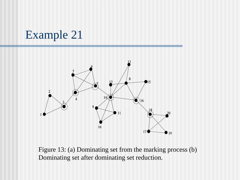
Example 21
Figure 13: (a) Dominating set from the marking process (b)
Dominating set after dominating set reduction.
Exercise 5
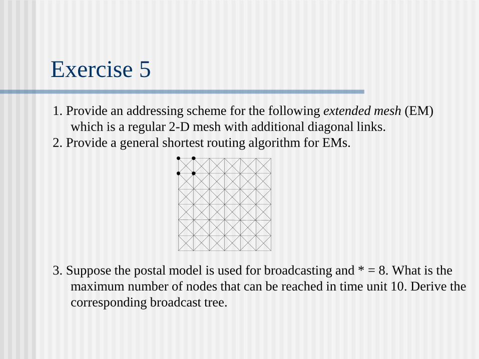
1. Provide an addressing scheme for the following extended mesh (EM)
which is a regular 2-D mesh with additional diagonal links.
2. Provide a general shortest routing algorithm for EMs.
3. Suppose the postal model is used for broadcasting and * = 8. What is the
maximum number of nodes that can be reached in time unit 10. Derive the
corresponding broadcast tree.

Exercise 5 (Cont’d)
4. Consider the following turn models:
West-first routing. Route a message first west, if necessary, and then adaptively south, east, and north.
North-last routing. First adaptively route a message south, east, and west; route the message north last.
Negative-first routing. First adaptively route a message along the negative X or Y axis; that is, south or west, then adaptively route the message along the positive X or Y axis.
Show all the turns allowed in each of the above three routings.
5. Show the corresponding routing paths using (1) positive-last, (2) west-first, (3) north-last, and (4) negative-first routing for the following unicasting:
6. Wu and Fernandez (1992) gave the following safe and unsafe node definition: A nonfaulty node is unsafe if and only if either of the following conditions is true: (a) There are two faulty neighbors, or (b) there are at least three unsafe or faulty neighbors. Consider a 4-cube with faulty nodes 0100, 0011, 0101, 1110, and 1111. Find out the safety status (safe or unsafe) of each node.
Exercise 5 (Cont’d)
7. To support fault-tolerant routing in 2-D meshes, D. J. Wang (1999)
proposed the following new model of faulty block: Suppose the
destination is in the first quadrant of the source. Initially, label all faulty
nodes as faulty and all non-faulty nodes as fault-free. If node u is fault-
free, but its north neighbor and east neighbor are faulty or useless, u is
labeled useless. If node u is fault-free, but its south neighbor and west
neighbor are faulty or can't-reach, u is labeled can't-reach. The nodes are
recursively labeled until there are no new useless or can't-reach nodes.
(a) Give an intuitive explanation of useless and can't-reach.
(b) Re-write the definition when the destination is in the second quadrant of the
source.
Exercise 5 (Cont’d)
8. Chiu proposed an odd-even turn model, which is an extension to Glass and Ni's turn model. The odd-even turn model tries to prevent the formation of the rightmost column segment of a cycle. Two rules for turn are given in:
Rule 1: Any packet is not allowed to take an EN (east-north) turn at any nodes located in an even column, and it is not allowed to take an NW turn at any nodes located in an odd column.
Rule 2: Any packet is not allowed to take an ES turn at any nodes located in an even column, and it is not allowed to take a SW turn at any nodes located in an odd column.
(a) Use your own word to explain that the odd-even turn model is deadlock-free.
(b) Show all the shortest paths (permissible under the extended odd-even turn model) for
(a) s1:(0, 0) and d1:(2,2) and (b) s2:(0,0) and d2:(3,2) (c) Prove Properties 1, 2, and 3 of Wu and Li's marking process for ad hoc
wireless networks.
Exercise 5 (Cont’d)
9. Suppose we use the following two rules to reduce
the size of the dominating set derived from Wu and
Li's marking process.
Rule 1: Consider two vertices v and u in G’. If N[v] N[u] in G and id(v) < id(u), change the marker of v to F if node v is marked, i.e., G' is changed to G'-{v},
Rule 2: Assume that u and w are two marked neighbors of marked vertex v in G'. If N(v) N(u) N(w) in G and id(v)= min{ id(v), id(u), id(w)}, then change the marker of v to F.
(1) Why id is used in both rules?
(2) If N[v] N[u] in G can Rule 1 be changed without checking the id's of v and u? (Consider two cases: (a) Rule 1 is used alone and (b) Rule 1 and Rule 2 are used together.)
Table of Contents
Introduction and Motivation
Theoretical Foundations
Distributed Programming Languages
Distributed Operating Systems
Distributed Communication
Distributed Data Management
Reliability
Applications
Conclusions
Appendix
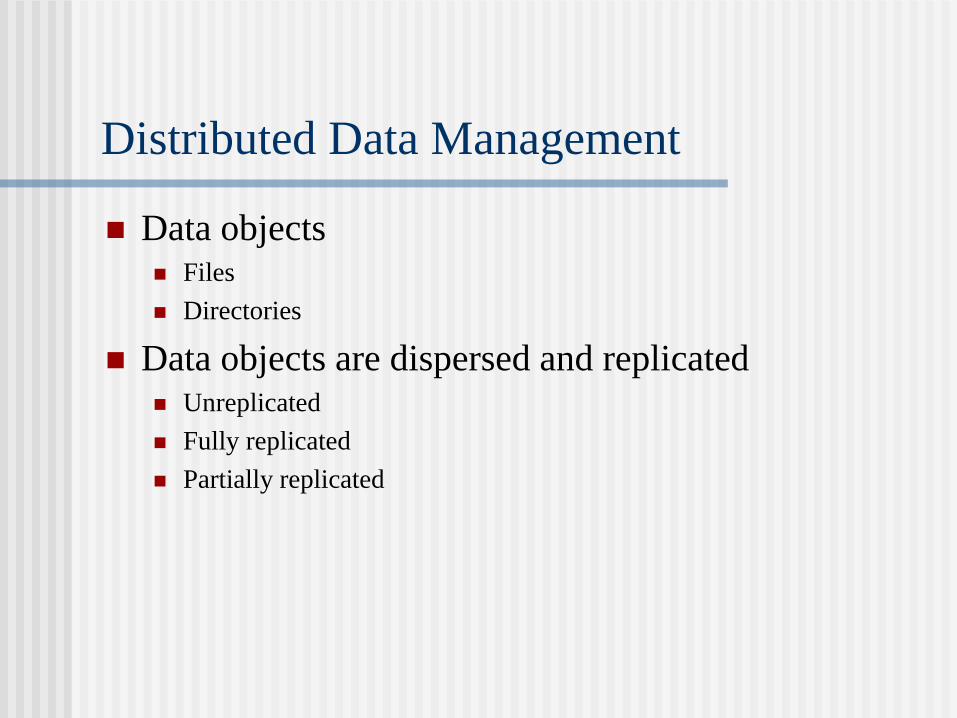
Distributed Data Management
Data objects Files
Directories
Data objects are dispersed and replicated Unreplicated
Fully replicated
Partially replicated

Serializability Theory
Atomic execution
A transaction is an "all or nothing" operation.
The concurrent execution of several transactions affects the
database as if executed serially in some order. The interleaved
order of the actions of a set of concurrent transactions is
called a schedule.
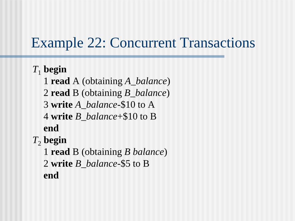
Example 22: Concurrent Transactions
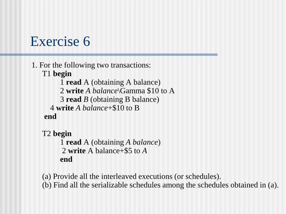
T1 begin
1 read A (obtaining A_balance)
2 read B (obtaining B_balance)
3 write A_balance-$10 to A
4 write B_balance+$10 to B
end
T2 begin
1 read B (obtaining B balance)
2 write B_balance-$5 to B
end
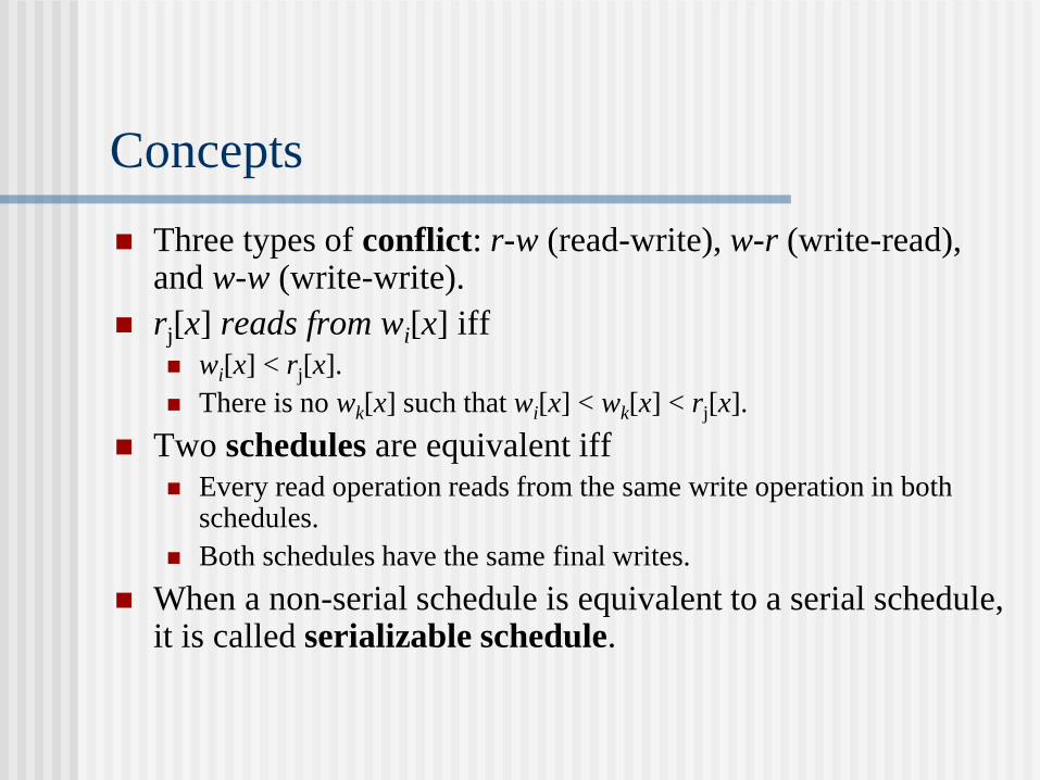
Three types of conflict: r-w (read-write), w-r (write-read), and w-w (write-write).
rj[x] reads from wi[x] iff
wi[x] < rj[x].
There is no wk[x] such that wi[x] < wk[x] < rj[x].
Two schedules are equivalent iff
Every read operation reads from the same write operation in both schedules.
Both schedules have the same final writes.
When a non-serial schedule is equivalent to a serial schedule, it is called serializable schedule.
Concepts
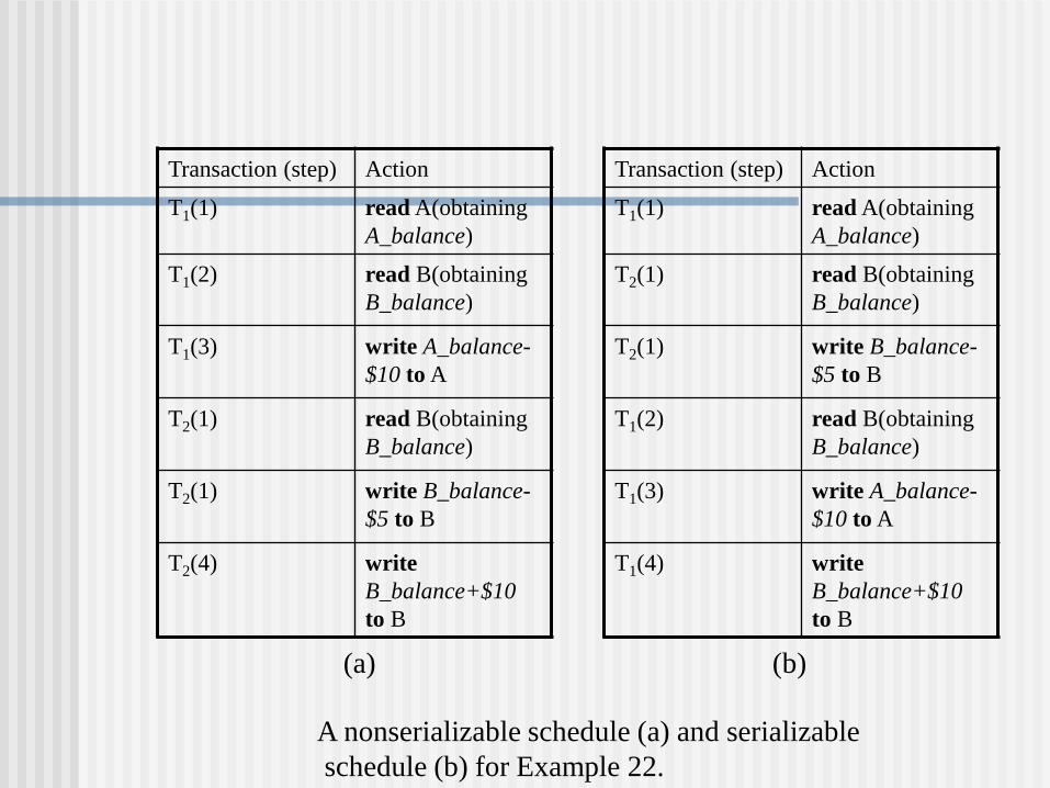
A nonserializable schedule (a) and serializable
schedule (b) for Example 22.
Transaction (step) Action
T1(1) read A(obtaining
A_balance)
T1(2)
read B(obtaining
B_balance)
T1(3)
write A_balance-
$10 to A
T2(1)
read B(obtaining
B_balance)
T2(1)
write B_balance-
$5 to B
T2(4)
write
B_balance+$10
to B
(a)
Transaction (step) Action
T1(1) read A(obtaining
A_balance)
T2(1)
read B(obtaining
B_balance)
T2(1)
write B_balance-
$5 to B
T1(2)
read B(obtaining
B_balance)
T1(3)
write A_balance-
$10 to A
T1(4)
write
B_balance+$10
to B
(b)
Concurrency Control
Locking scheme
Timestamp-based scheme
Optimistic concurrency control
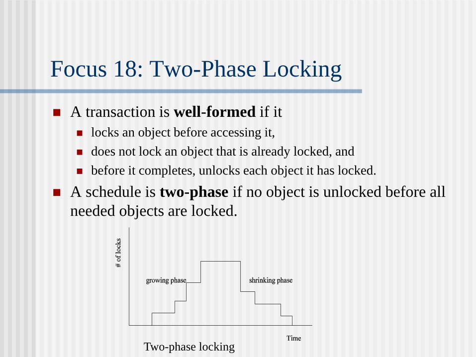
Focus 18: Two-Phase Locking
A transaction is well-formed if it
locks an object before accessing it,
does not lock an object that is already locked, and
before it completes, unlocks each object it has locked.
A schedule is two-phase if no object is unlocked before all
needed objects are locked.
Two-phase locking
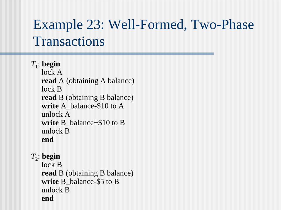
Example 23: Well-Formed, Two-Phase
Transactions
T1: begin lock A read A (obtaining A balance) lock B read B (obtaining B balance) write A_balance-$10 to A unlock A write B_balance+$10 to B unlock B end T2: begin lock B read B (obtaining B balance) write B_balance-$5 to B unlock B end
Different Looking Schemes
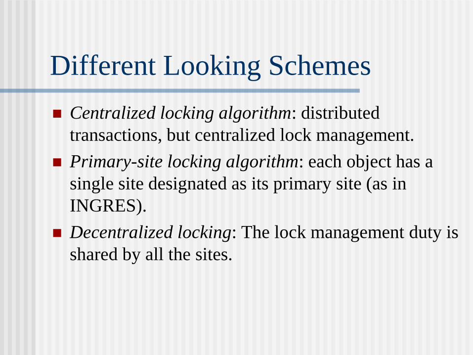
Centralized locking algorithm: distributed
transactions, but centralized lock management.
Primary-site locking algorithm: each object has a
single site designated as its primary site (as in
INGRES).
Decentralized locking: The lock management duty is
shared by all the sites.
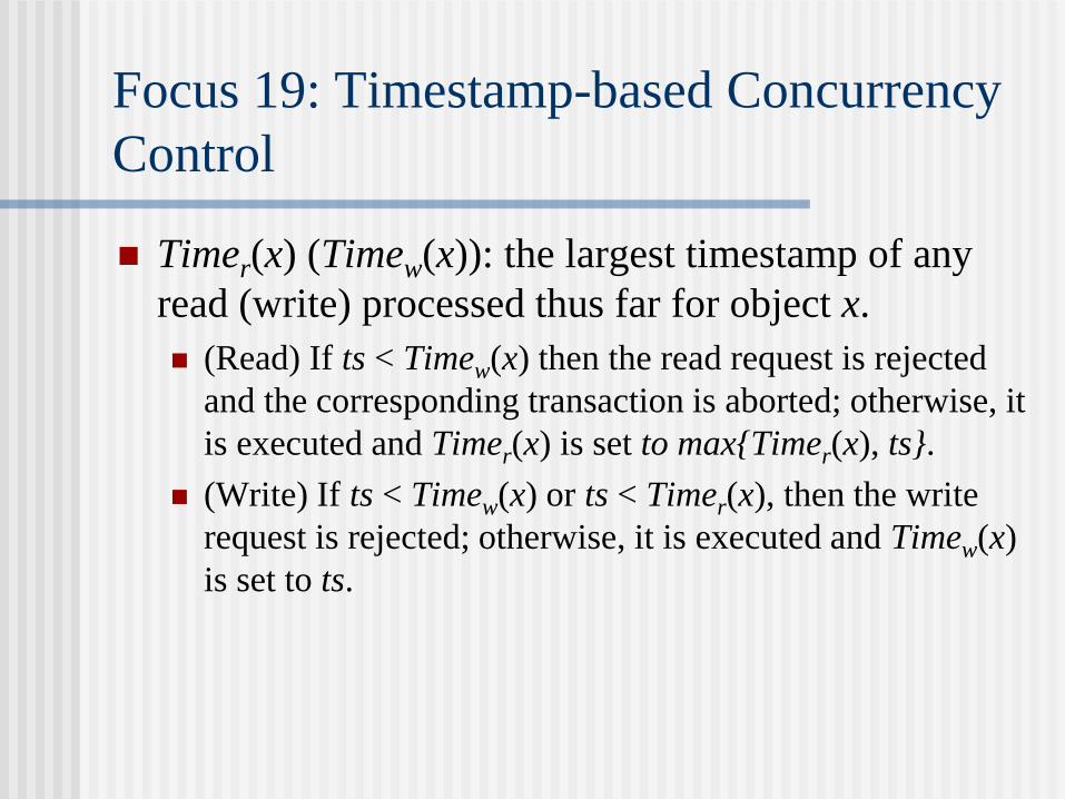
Focus 19: Timestamp-based Concurrency
Control
Timer(x) (Timew(x)): the largest timestamp of any
read (write) processed thus far for object x.
(Read) If ts < Timew(x) then the read request is rejected
and the corresponding transaction is aborted; otherwise, it
is executed and Timer(x) is set to max{Timer(x), ts}.
(Write) If ts < Timew(x) or ts < Timer(x), then the write
request is rejected; otherwise, it is executed and Timew(x)
is set to ts.
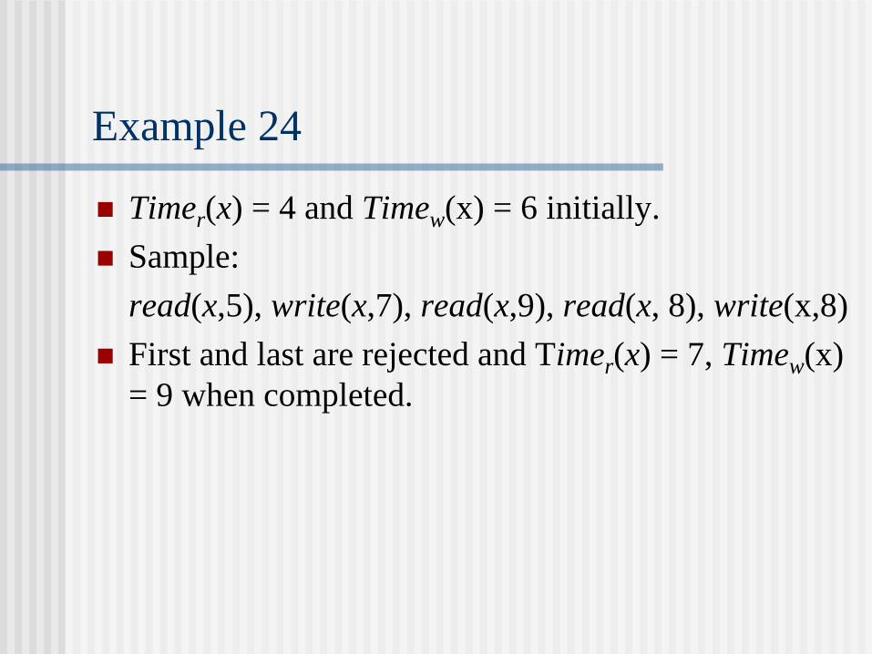
Example 24
Timer(x) = 4 and Timew(x) = 6 initially.
Sample:
read(x,5), write(x,7), read(x,9), read(x, 8), write(x,8)
First and last are rejected and Timer(x) = 7, Timew(x)
= 9 when completed.

Conservative Timestamp Ordering
Each site keeps a write queue (W-queue) and a read
queue (R-queue).
A read (x, ts) request is executed if all W-queues are
nonempty and the first write on each queue has a
timestamp greater than ts; otherwise, the read request is
buffered in the R-queue.
A write (x, ts) request is executed if all R-queues and W–
queues are nonempty and the first read (write) on each R-
queue (W-queue) has a timestamp greater than ts;
otherwise, the write request is buffered in the W-queue.
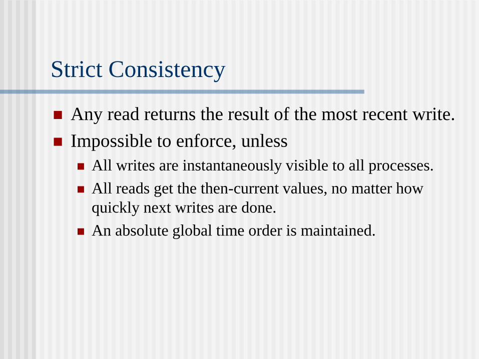
Strict Consistency
Any read returns the result of the most recent write.
Impossible to enforce, unless
All writes are instantaneously visible to all processes.
All reads get the then-current values, no matter how
quickly next writes are done.
An absolute global time order is maintained.
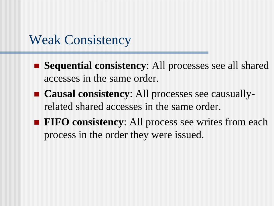
Weak Consistency
Sequential consistency: All processes see all shared
accesses in the same order.
Causal consistency: All processes see causually-
related shared accesses in the same order.
FIFO consistency: All process see writes from each
process in the order they were issued.

Weak consistency: Enforces consistency on a group
of operations, not on individual reads and writes.
Release consistency: Enforces consistency on a
group of operations enclosed by acquire and release
operations.
Eventual consistency: All replicas will gradually
become consistent. (Web pages with dominated read
operations.)
Weak Consistency (Cont’d)
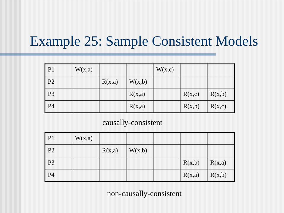
Example 25: Sample Consistent Models
causally-consistent
P1 W(x,a) W(x,c)
P2 R(x,a) W(x,b)
P3 R(x,a) R(x,c) R(x,b)
P4 R(x,a) R(x,b) R(x,c)
P1 W(x,a)
P2 R(x,a) W(x,b)
P3 R(x,b) R(x,a)
P4 R(x,a) R(x,b)
non-causally-consistent
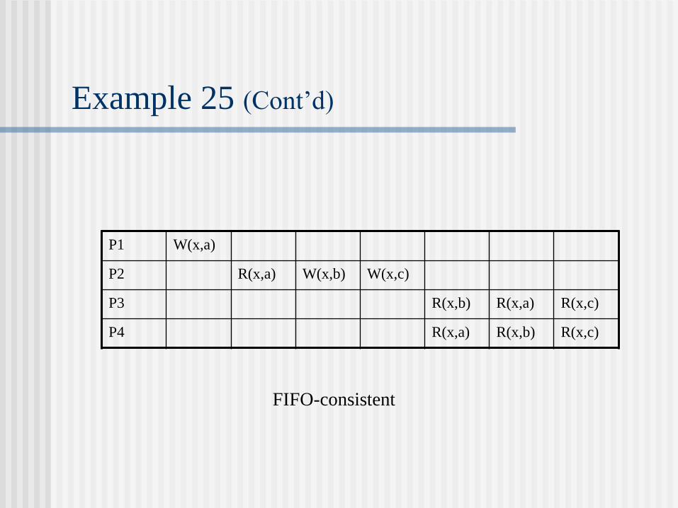
Example 25 (Cont’d)
FIFO-consistent
P1 W(x,a)
P2 R(x,a) W(x,b) W(x,c)
P3 R(x,b) R(x,a) R(x,c)
P4 R(x,a) R(x,b) R(x,c)
Update Propagation
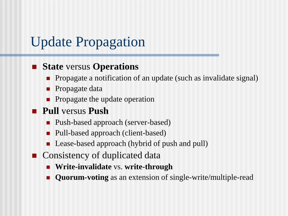
State versus Operations
Propagate a notification of an update (such as invalidate signal)
Propagate data
Propagate the update operation
Pull versus Push
Push-based approach (server-based)
Pull-based approach (client-based)
Lease-based approach (hybrid of push and pull)
Consistency of duplicated data
Write-invalidate vs. write-through
Quorum-voting as an extension of single-write/multiple-read
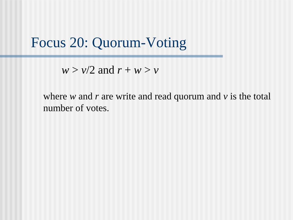
Focus 20: Quorum-Voting
w > v/2 and r + w > v
where w and r are write and read quorum and v is the total
number of votes.
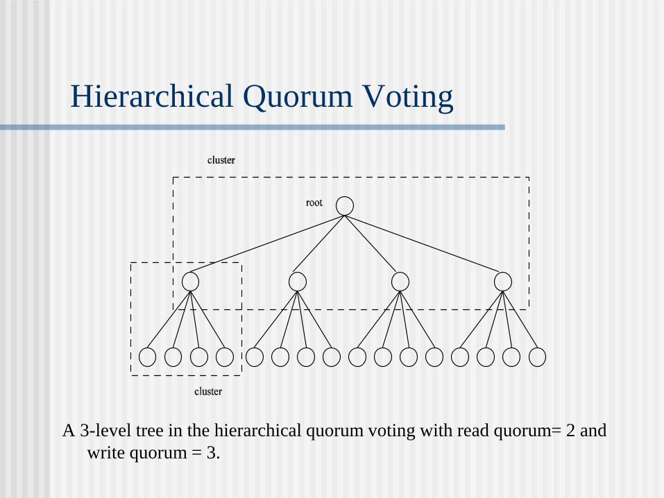
Hierarchical Quorum Voting
A 3-level tree in the hierarchical quorum voting with read quorum= 2 and
write quorum = 3.

Gray's Two-Phase Commitment Protocol
The finite state machine model for the
two-phase commit protocol.
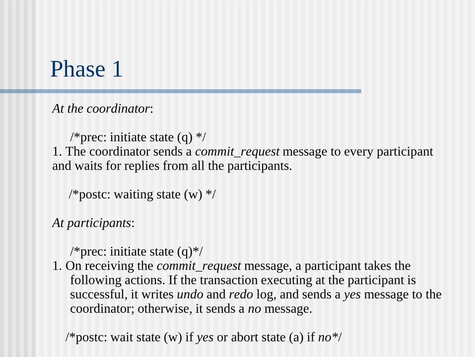
Phase 1
At the coordinator: /*prec: initiate state (q) */ 1. The coordinator sends a commit_request message to every participant and waits for replies from all the participants. /*postc: waiting state (w) */ At participants: /*prec: initiate state (q)*/ 1. On receiving the commit_request message, a participant takes the
following actions. If the transaction executing at the participant is successful, it writes undo and redo log, and sends a yes message to the coordinator; otherwise, it sends a no message.
/*postc: wait state (w) if yes or abort state (a) if no*/
Phase 2
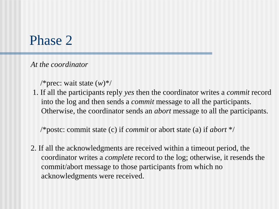
At the coordinator
/*prec: wait state (w)*/
1. If all the participants reply yes then the coordinator writes a commit record
into the log and then sends a commit message to all the participants.
Otherwise, the coordinator sends an abort message to all the participants.
/*postc: commit state (c) if commit or abort state (a) if abort */
2. If all the acknowledgments are received within a timeout period, the
coordinator writes a complete record to the log; otherwise, it resends the
commit/abort message to those participants from which no
acknowledgments were received.
Phase 2 (Cont’d)
At the participants /*prec: wait state (w) */ 1. On receiving a commit message, a participant releases all the resources and
locks held for executing the transaction and sends an acknowledgment. /*postc: commit state (c) */ /*prec: abort state (a) or wait state (w) */ 2. On receiving an abort message, a participant undoes the transaction using
the undo log record, releases all the resources and locks held by it, and sends an acknowledgment.
/*postc: abort state (a) */
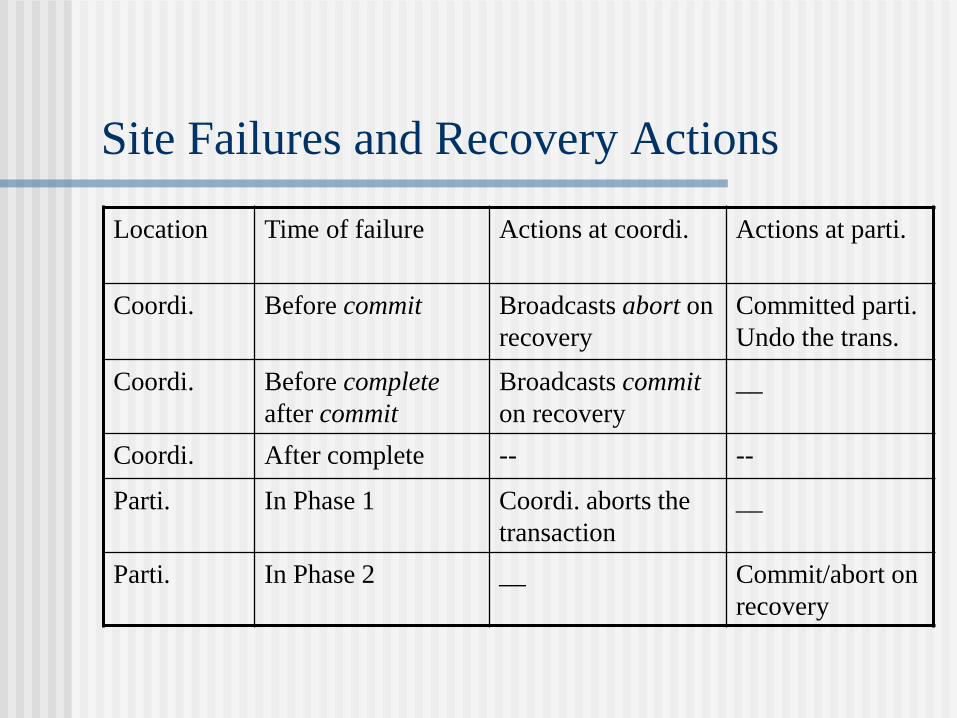
Site Failures and Recovery Actions
Location Time of failure Actions at coordi. Actions at parti.
Coordi. Before commit Broadcasts abort on
recovery
Committed parti.
Undo the trans.
Coordi. Before complete
after commit
Broadcasts commit
on recovery
__
Coordi. After complete -- --
Parti. In Phase 1 Coordi. aborts the
transaction
__
Parti. In Phase 2 __ Commit/abort on
recovery
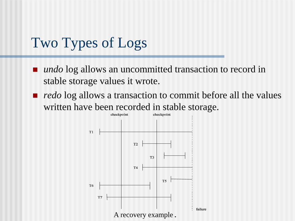
Two Types of Logs
undo log allows an uncommitted transaction to record in
stable storage values it wrote.
redo log allows a transaction to commit before all the values
written have been recorded in stable storage.
A recovery example.
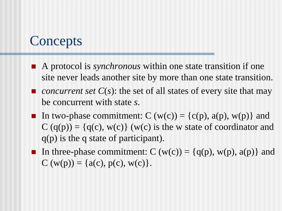
A protocol is synchronous within one state transition if one
site never leads another site by more than one state transition.
concurrent set C(s): the set of all states of every site that may
be concurrent with state s.
In two-phase commitment: C (w(c)) = {c(p), a(p), w(p)} and
C (q(p)) = {q(c), w(c)} (w(c) is the w state of coordinator and
q(p) is the q state of participant).
In three-phase commitment: C (w(c)) = {q(p), w(p), a(p)} and
C (w(p)) = {a(c), p(c), w(c)}.
Concepts
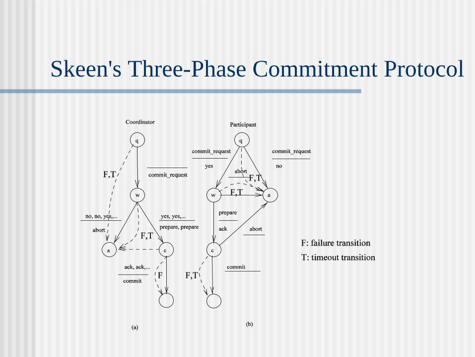
Skeen's Three-Phase Commitment Protocol
Exercise 6
1. For the following two transactions: T1 begin 1 read A (obtaining A balance) 2 write A balance\Gamma $10 to A 3 read B (obtaining B balance) 4 write A balance+$10 to B end T2 begin 1 read A (obtaining A balance) 2 write A balance+$5 to A end (a) Provide all the interleaved executions (or schedules). (b) Find all the serializable schedules among the schedules obtained in (a).
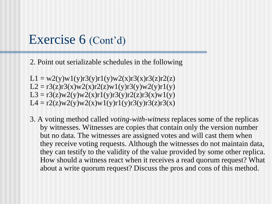
Exercise 6 (Cont’d)
2. Point out serializable schedules in the following L1 = w2(y)w1(y)r3(y)r1(y)w2(x)r3(x)r3(z)r2(z) L2 = r3(z)r3(x)w2(x)r2(z)w1(y)r3(y)w2(y)r1(y) L3 = r3(z)w2(y)w2(x)r1(y)r3(y)r2(z)r3(x)w1(y) L4 = r2(z)w2(y)w2(x)w1(y)r1(y)r3(y)r3(z)r3(x) 3. A voting method called voting-with-witness replaces some of the replicas
by witnesses. Witnesses are copies that contain only the version number but no data. The witnesses are assigned votes and will cast them when they receive voting requests. Although the witnesses do not maintain data, they can testify to the validity of the value provided by some other replica. How should a witness react when it receives a read quorum request? What about a write quorum request? Discuss the pros and cons of this method.
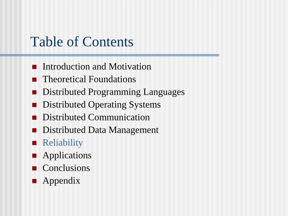
Table of Contents
Introduction and Motivation
Theoretical Foundations
Distributed Programming Languages
Distributed Operating Systems
Distributed Communication
Distributed Data Management
Reliability
Applications
Conclusions
Appendix

Type of Faults
Types of faults:
Hardware faults
Software faults
Communication faults
Timing faults
Schneider’s classification:
Omission failure
Failstop failure (detectable)
Crash failure (undetectable)
Crash and link failure
Byzantine failure

Redundancy
Hardware redundancy: extra PE's, I/O's
Software redundancy: extra version of software modules
Information redundancy: error detecting code
Time redundancy: additional time used to perform a
function
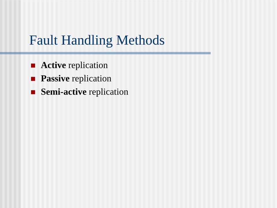
Fault Handling Methods
Active replication
Passive replication
Semi-active replication

Building Blocks of Fault-Tolerant Design
Stable storage is a logical abstraction for a special storage
that can survive system failure.
Fail-stop processors do not perform any incorrect action and
simply cease to function.
An atomic action is a set of operations which are executed
indivisibly by hardware. That is, either operations are
completed successfully and fully or the state of the system
remains unchanged (operations are not executed at all).
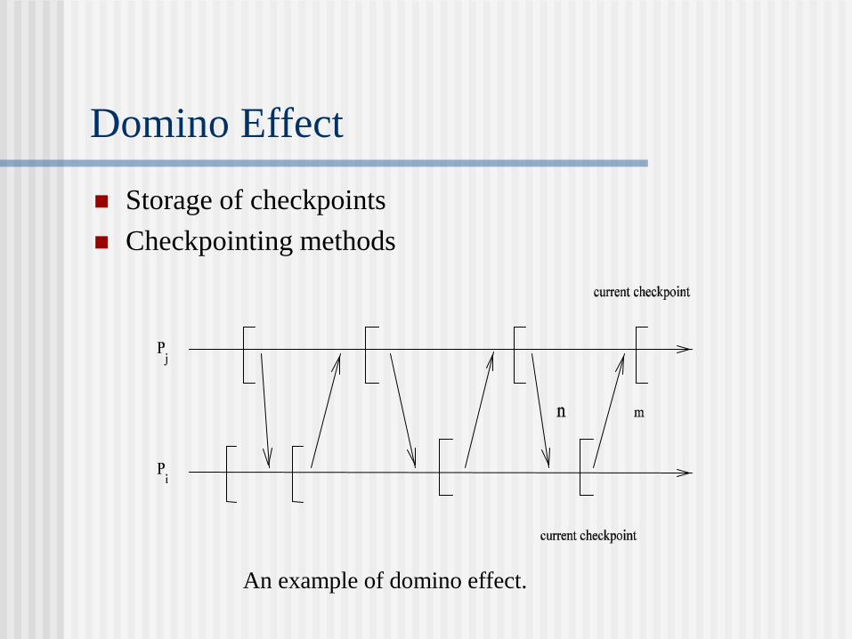
Storage of checkpoints
Checkpointing methods
An example of domino effect.
Domino Effect
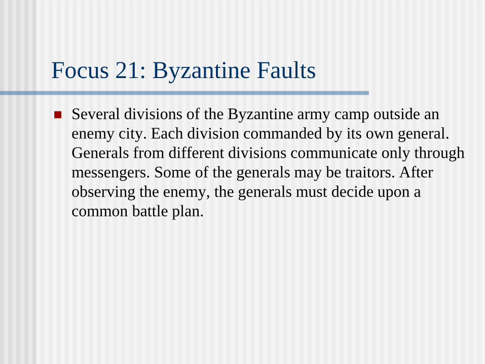
Focus 21: Byzantine Faults
Several divisions of the Byzantine army camp outside an
enemy city. Each division commanded by its own general.
Generals from different divisions communicate only through
messengers. Some of the generals may be traitors. After
observing the enemy, the generals must decide upon a
common battle plan.

Two Requirements
All loyal generals decide upon the same plan of action
A small number of traitors cannot cause the loyal generals to
adopt a wrong plan
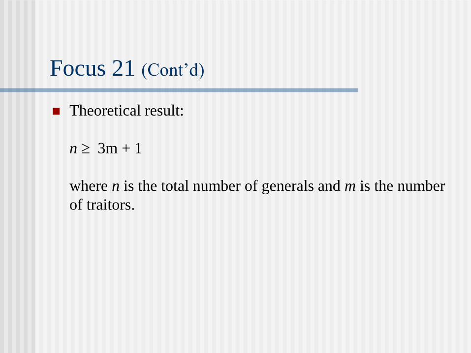
Focus 21 (Cont’d)
Theoretical result:
n 3m + 1
where n is the total number of generals and m is the number
of traitors.

Agreement Protocol
An algorithm for reaching agreement.
P1* P2 P3 P4
First round:
(-,v2,v3,v4)
(v12, -,v3, v4)
(v11,v2,- v4)
(v13,v2, v3,-)
Second round:
(v12, -, v3, v4)
(v11, v2, -, v4)
(v13, v2, v3, -)
(v11, v2, -, v4)
(v13, v2, v3, -)
(-, v24, v3
4, v44)
(v11, -, v3, v4)
(v13, v2, v3, -)
(-, v25, v3
5, v45)
(v12, -, v3, v4)
(v11, v2, -, v4)
(-, v26, v3
6, v46)
(d1, d2,d3, d4) (v17, v2, v3, v4) (v1
7, v2, v3, v4) (v17, v2, v3, v4)
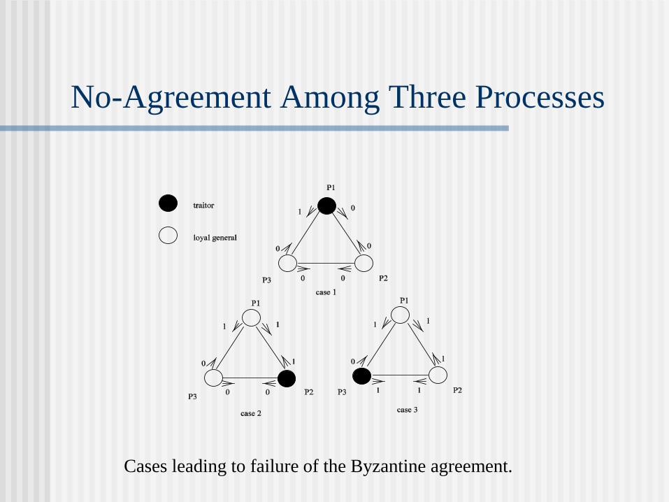
No-Agreement Among Three Processes
Cases leading to failure of the Byzantine agreement.
Extended Agreement Protocols
Boolean values or arbitrary real values for the decisions.
Unauthenticated or authenticated messages.
Synchronous or asynchronous.
Completely connected network or partially connected networks.
Deterministic or randomized.
Byzantine faults or fail-stop faults.
Non-totally decentralized control system and, in particular, hierarchical control systems.

Reliable Communication
Acknowledgement: acknowledge the receipt of each packet.
TCP: transport protocol for reliable point-to-point comm.
Negative acknowledgement
Signal for a missing packet.
Pros: better scalability (without positive acknowledgement).
Cons: sender is forced to keep each packet in the buffer forever.
Reliable Group Communication
Feedback suppression: multicast or broadcast each positive
(or negative) acknowledge.
Combination of positive and negative acknowledgements
Example 26: Combination of Positive and
Negative Acknowledgements in Broadcasting.
Let A be a packet and a (a) the positive (negative) acknowledgement for A. A,Ba,Cb,Db,Ec,F cd,Cb,Gdef
1.Message A is sent first, acknowledged by the sender of B, which is in turn acknowledged by the senders of C and D. 2. The sender of E acknowledges C and the sender of F acknowledges the receipt of D but a negative acknowledgment of C . 3. Some node (not necessarily the original sender) retransmits C .
4. The sender of G acknowledges both E and F but sends a negative acknowledgment of D (after receiving F ).

Different Types of Reliable Multicasting
Reliable multicast: no message ordering
FIFO multicast: FIFO-ordered delivery
Causal multicast: causal-ordered delivery
Atomic multicast: reliable multicast + total-ordered delivery
FIFO atomic multicast: FIFO multicast + total-ordered
delivery
Causal atomic multicast: Causal multicast + total-ordered
delivery
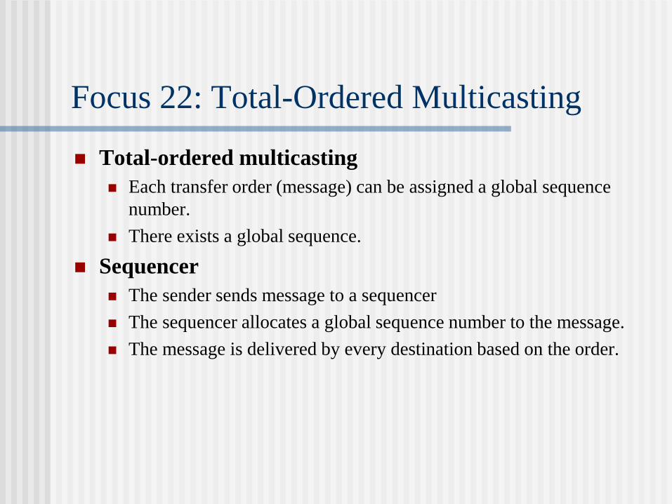
Focus 22: Total-Ordered Multicasting
Total-ordered multicasting
Each transfer order (message) can be assigned a global sequence
number.
There exists a global sequence.
Sequencer
The sender sends message to a sequencer
The sequencer allocates a global sequence number to the message.
The message is delivered by every destination based on the order.
Implementations of Sequencer
Privilege-based (token circulated among the senders)
Fixed sequencer (a fixed third party)
Moving sequencer(token circulated among the third-party
nodes)
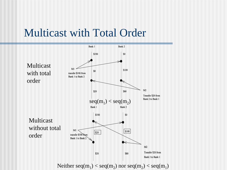
Multicast with Total Order
seq(m1) < seq(m2)
Neither seq(m1) < seq(m2) nor seq(m2) < seq(m1)
Multicast
with total
order
Multicast
without total
order
Focus 23: Birman’s Virtual Synchrony
Virtual synchrony: reliable multicast with a special property.
View: a multicast group.
View change: (a) a new process joins, (b) a process leaves, and (c) a process crashes.
Each view change is multicast to members in the group.
Special property: each view change acts as a barrier across which no multicast can pass. (Application: distributed debugging.)

Focus 23 (Cont’d)
Virtual synchrony.
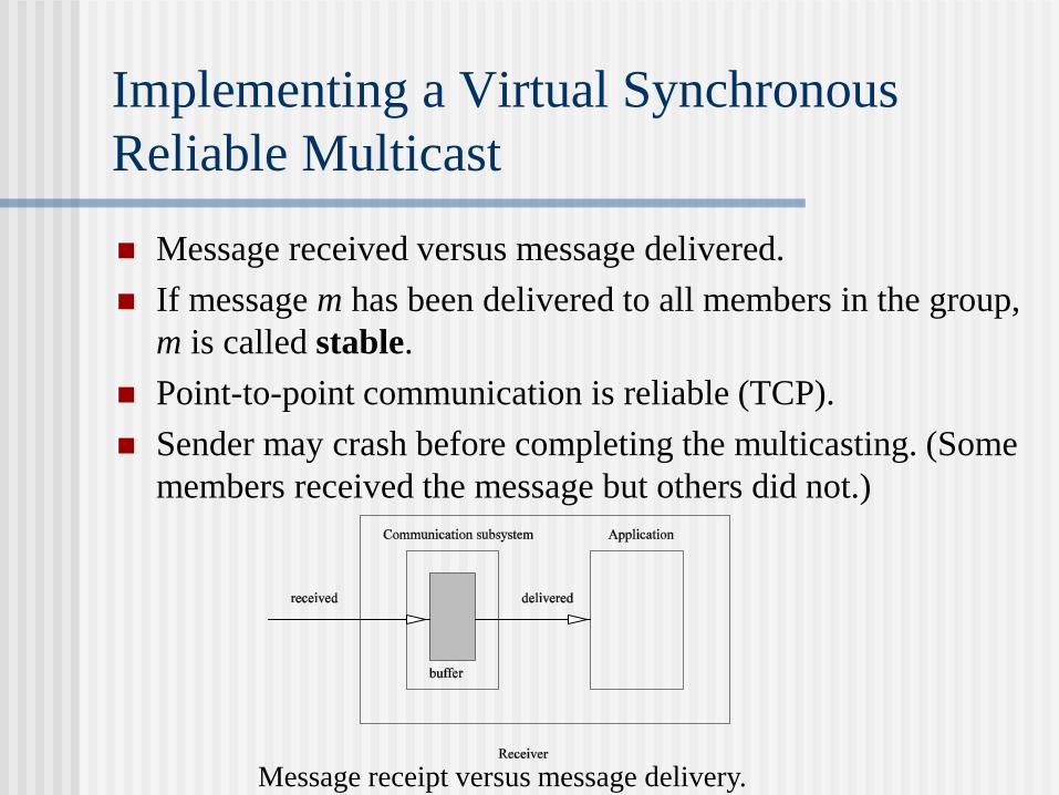
Implementing a Virtual Synchronous
Reliable Multicast
Message received versus message delivered.
If message m has been delivered to all members in the group,
m is called stable.
Point-to-point communication is reliable (TCP).
Sender may crash before completing the multicasting. (Some
members received the message but others did not.)
Message receipt versus message delivery.
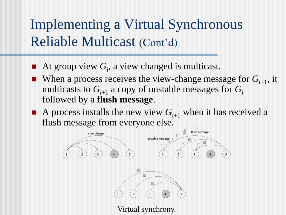
At group view Gi, a view changed is multicast.
When a process receives the view-change message for Gi+1, it multicasts to Gi+1 a copy of unstable messages for Gi followed by a flush message.
A process installs the new view Gi+1 when it has received a flush message from everyone else.
Virtual synchrony.
Implementing a Virtual Synchronous
Reliable Multicast (Cont’d)
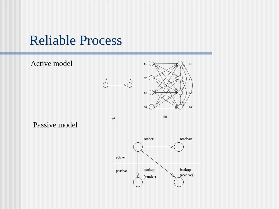
Reliable Process
Active model
Passive model
Exercise 7
1. Use a practical example to illustrate the differences among faults, errors, and failures.
2. Illustrate the correctness of the agreement protocol for authenticated messages using a system of four processes with two faulty processes. You need to consider the following two cases: The sender is healthy and two receivers are faulty (the remaining receiver is healthy).
The sender is faulty and one receiver is faulty (the remaining receivers are healthy).
3. In Byzantine agreement protocol k + 1 rounds of message exchanges are needed to tolerant k faults. The number of processes n is at least 3k + 1. Assume P1 and P2 are faulty in a system of n = 7 processes.
(a) Show the messages P3 receives in first, second, and third round.
(b) Demonstrate the correctness of the protocol by showing the final result vector (after a majority voting) for P3.
(c) Briefly show that result vectors for other non-faulty processes are the same.

Table of Contents
Introduction and Motivation
Theoretical Foundations
Distributed Programming Languages
Distributed Operating Systems
Distributed Communication
Distributed Data Management
Reliability
Applications
Conclusions
Appendix
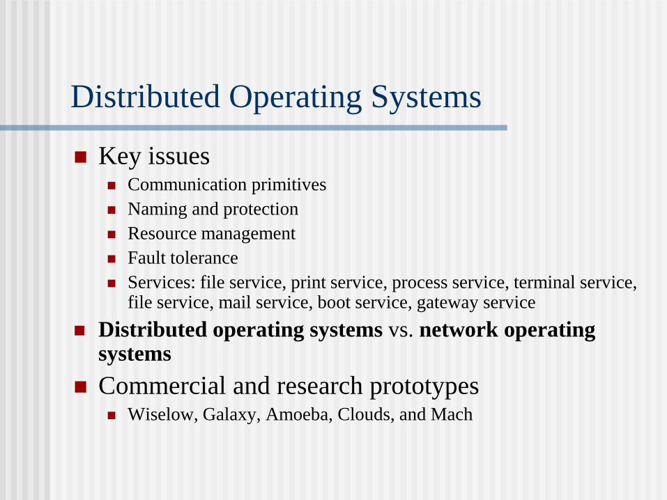
Distributed Operating Systems
Key issues Communication primitives
Naming and protection
Resource management
Fault tolerance
Services: file service, print service, process service, terminal service, file service, mail service, boot service, gateway service
Distributed operating systems vs. network operating systems
Commercial and research prototypes
Wiselow, Galaxy, Amoeba, Clouds, and Mach
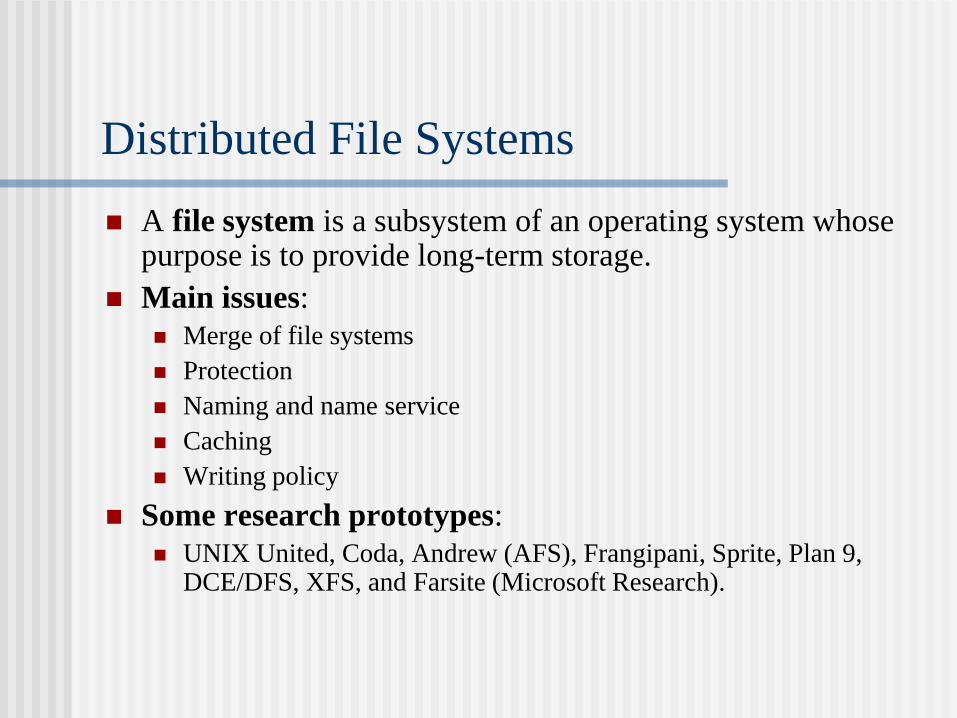
Distributed File Systems
A file system is a subsystem of an operating system whose purpose is to provide long-term storage.
Main issues:
Merge of file systems
Protection
Naming and name service
Caching
Writing policy
Some research prototypes:
UNIX United, Coda, Andrew (AFS), Frangipani, Sprite, Plan 9, DCE/DFS, XFS, and Farsite (Microsoft Research).
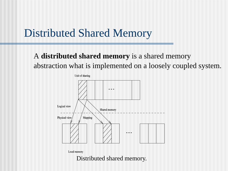
Distributed Shared Memory
A distributed shared memory is a shared memory
abstraction what is implemented on a loosely coupled system.
Distributed shared memory.

Focus 24: Stumm and Zhou's Classification
Central-server algorithm (nonmigrating and
nonreplicated).
(Client) Sends a data request to the central server.
(Central server) Receives the request, performs data
access and
sends a response.
(Client) Receives the response.
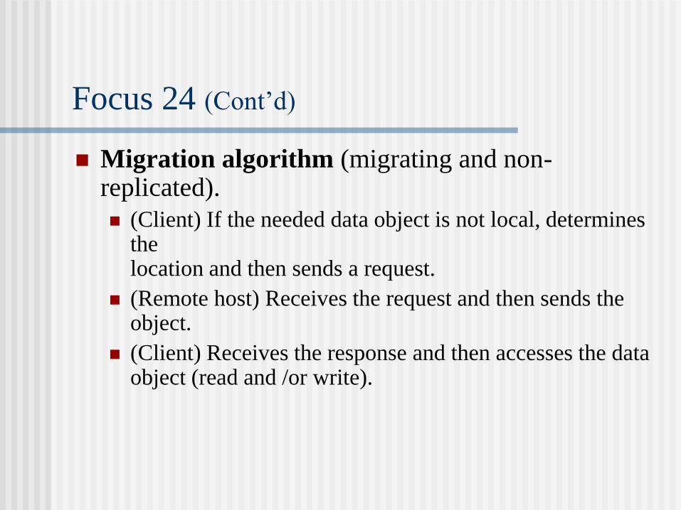
Focus 24 (Cont’d)
Migration algorithm (migrating and non-replicated).
(Client) If the needed data object is not local, determines the location and then sends a request.
(Remote host) Receives the request and then sends the object.
(Client) Receives the response and then accesses the data object (read and /or write).
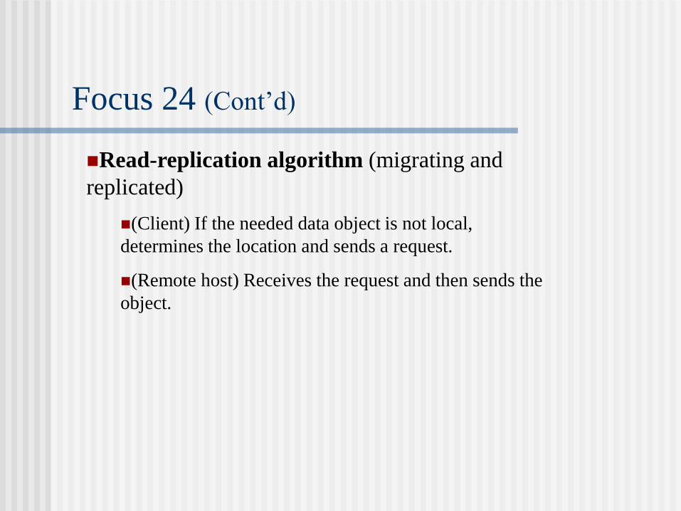
Focus 24 (Cont’d)
Read-replication algorithm (migrating and
replicated)
(Client) If the needed data object is not local,
determines the location and sends a request.
(Remote host) Receives the request and then sends the
object.
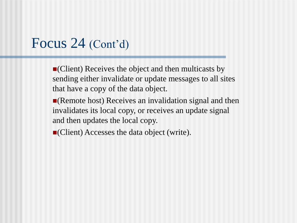
Focus 24 (Cont’d)
(Client) Receives the object and then multicasts by
sending either invalidate or update messages to all sites
that have a copy of the data object.
(Remote host) Receives an invalidation signal and then
invalidates its local copy, or receives an update signal
and then updates the local copy.
(Client) Accesses the data object (write).
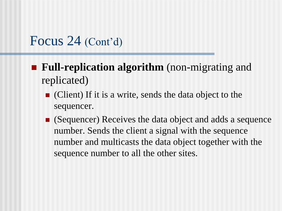
Focus 24 (Cont’d)
Full-replication algorithm (non-migrating and
replicated)
(Client) If it is a write, sends the data object to the
sequencer.
(Sequencer) Receives the data object and adds a sequence
number. Sends the client a signal with the sequence
number and multicasts the data object together with the
sequence number to all the other sites.
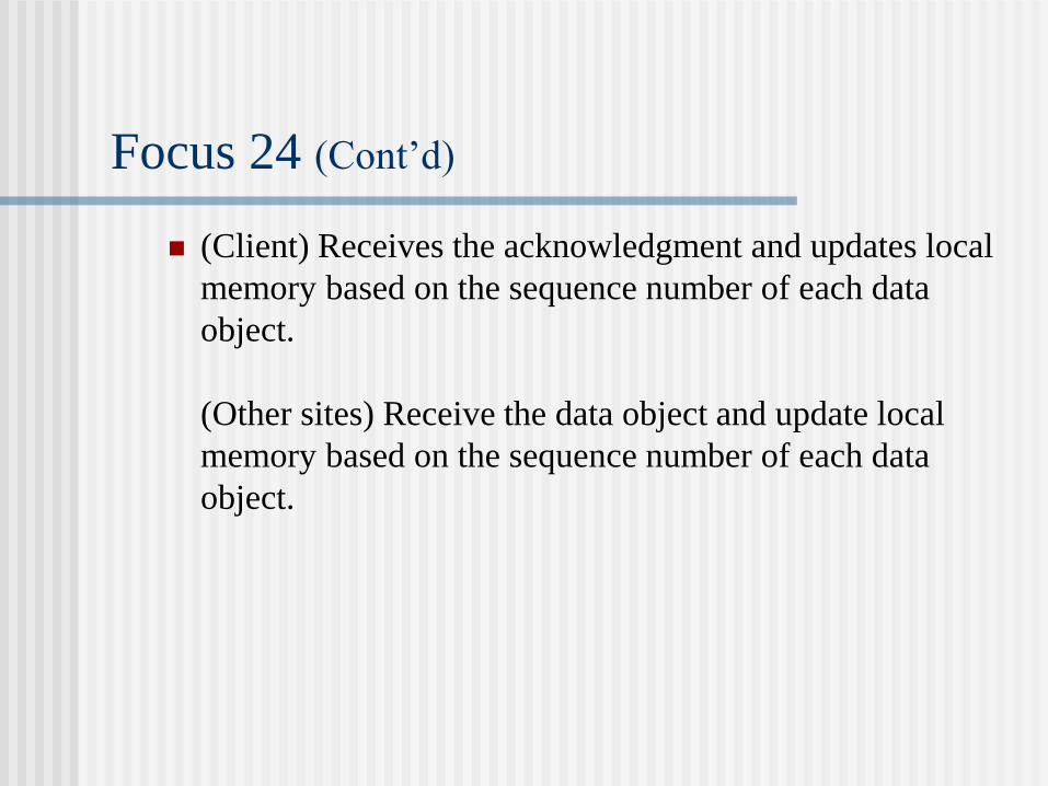
Focus 24 (Cont’d)
(Client) Receives the acknowledgment and updates local
memory based on the sequence number of each data
object.
(Other sites) Receive the data object and update local
memory based on the sequence number of each data
object.
Focus 24 (Cont’d)
Main Issues:
Structure and granularity
Coherence semantics
Scalability
Heterogeneity
Several research prototypes:
Dash, Ivy, Munin, and Clouds
Alewife (MIT), Treadmarks (Rice), Coherent Virtual machine
(Maryland), and Millipede (Israel Inst. Tech.)
Distributed Database Systems
A distributed database is a collection of multiple, logically interrelated databases distributed over a computer network.
Possible design alternatives:
Autonomy
Distribution
Heterogeneity
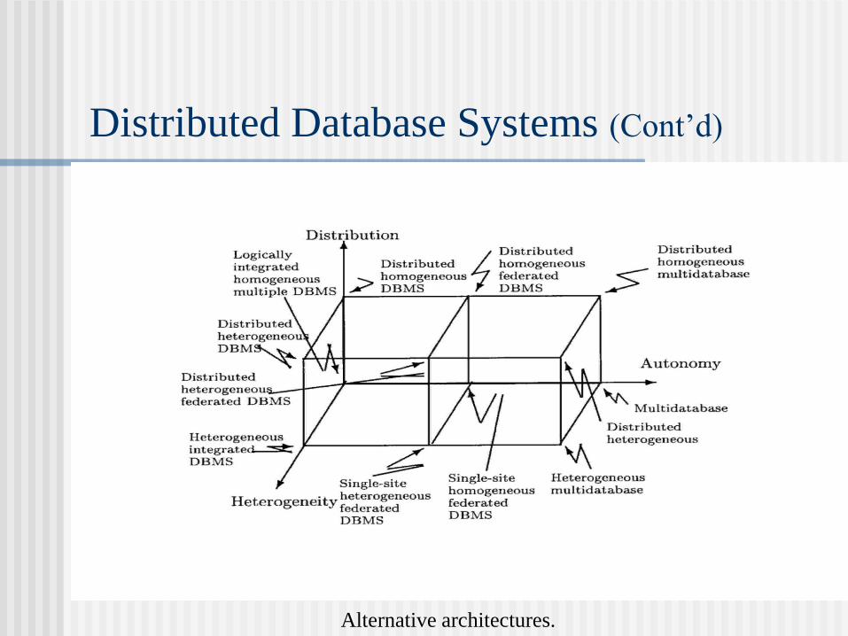
Distributed Database Systems (Cont’d)
Alternative architectures.

Essentials of Distributed Database Systems
Local autonomy
No reliance on a central site
Continuous operation
Location independence
Fragment independence
Replication independence
Distributed query processing
Distributed transaction management
Hardware independence
Operating system independence
Network independence
Data independence

Network scaling problem
Distributed query processing
Integration with distributed operating systems
Heterogeneity
Concurrency control
Security
Next-generation database systems:
Object-oriented database management systems
Knowledge base management systems
Open Research Problems
ADDS (Amocha Distributed Database Systems)
JDDBS (Japanese Distributed Database Systems)
Ingres/star
SWIFT (Society for Worldwide Interbank Financial Financial Telecommunication)
System R
MYRIAD
MULTIBASE
MERMAID
Research Prototypes and Commercial
Products
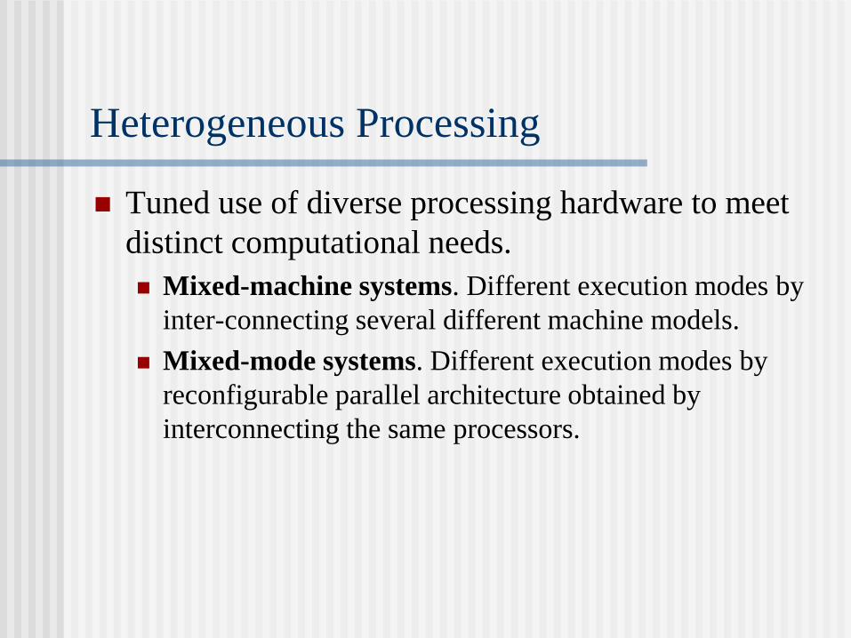
Heterogeneous Processing
Tuned use of diverse processing hardware to meet
distinct computational needs.
Mixed-machine systems. Different execution modes by
inter-connecting several different machine models.
Mixed-mode systems. Different execution modes by
reconfigurable parallel architecture obtained by
interconnecting the same processors.
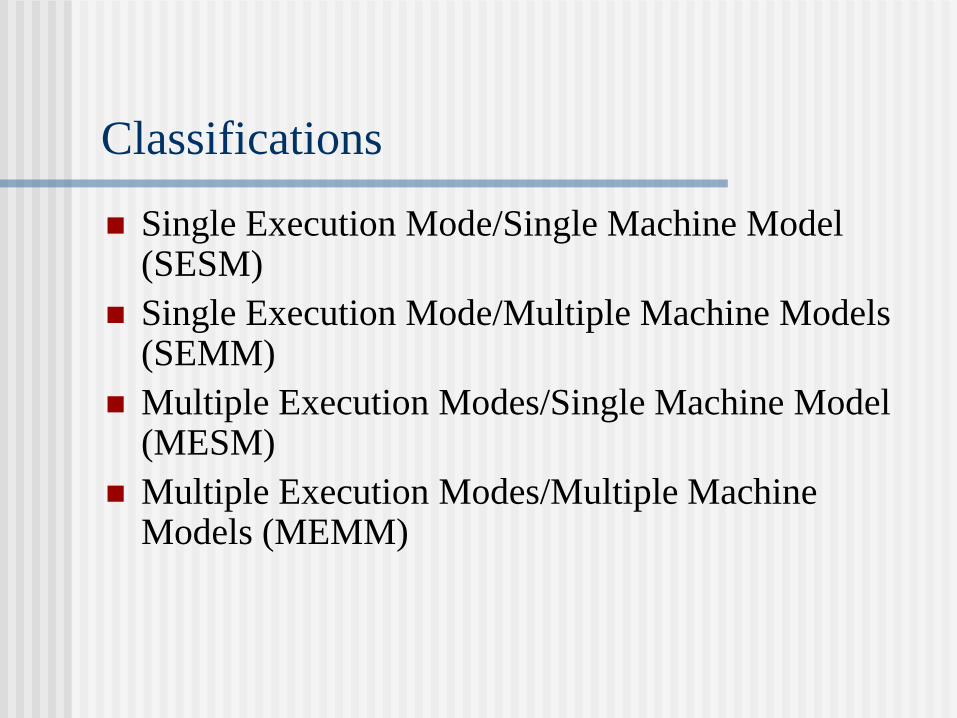
Classifications
Single Execution Mode/Single Machine Model (SESM)
Single Execution Mode/Multiple Machine Models (SEMM)
Multiple Execution Modes/Single Machine Model (MESM)
Multiple Execution Modes/Multiple Machine Models (MEMM)
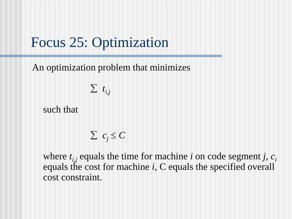
Focus 25: Optimization
An optimization problem that minimizes ti,j such that
cj C where ti,j equals the time for machine i on code segment j, ci equals the cost for machine i, C equals the specified overall cost constraint.

Table of Contents
Introduction and Motivation
Theoretical Foundations
Distributed Programming Languages
Distributed Operating Systems
Distributed Communication
Distributed Data Management
Reliability
Applications
Conclusions
Appendix
"Killer" Applications
Distributed Object-based Systems: CORBA
Distributed Document-based Systems: WWW
Distributed Coordination-based Systems: JINI
Distributed Multimedia Systems: QoS requirements
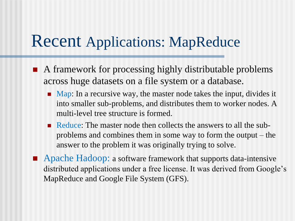
Recent Applications: MapReduce
A framework for processing highly distributable problems
across huge datasets on a file system or a database.
Map: In a recursive way, the master node takes the input, divides it
into smaller sub-problems, and distributes them to worker nodes. A
multi-level tree structure is formed.
Reduce: The master node then collects the answers to all the sub-
problems and combines them in some way to form the output – the
answer to the problem it was originally trying to solve.
Apache Hadoop: a software framework that supports data-intensive
distributed applications under a free license. It was derived from Google’s
MapReduce and Google File System (GFS).
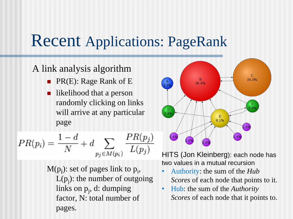
Recent Applications: PageRank
A link analysis algorithm
PR(E): Rage Rank of E
likelihood that a person
randomly clicking on links
will arrive at any particular
page
M(pi): set of pages link to pi,
L(pj): the number of outgoing
links on pj, d: dumping
factor, N: total number of
pages.
HITS (Jon Kleinberg): each node has
two values in a mutual recursion
• Authority: the sum of the Hub
Scores of each node that points to it.
• Hub: the sum of the Authority
Scores of each node that it points to.

Emerging Systems
Wireless networks and mobile computing: mobile agents
Move the computation to the data rather than the data to the
computations.
Grid
TeraGrid: 13.6 teraflops of Linux Cluster computing power
distributed at the four TeraGrid sites.
Open Grid Services Architecture (OGSA): delivering tighter
integration between grid computing networks and Web services
technologies.
Grid Computing (via OGSA) as the basis of evolution of Internet
computing in the future.
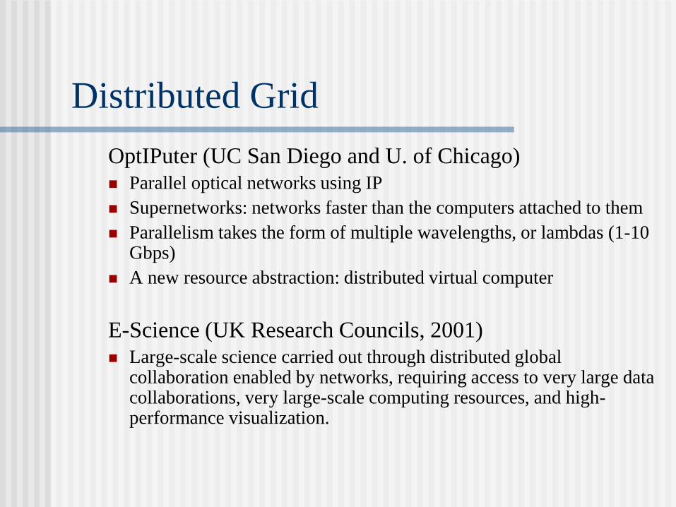
Distributed Grid
OptIPuter (UC San Diego and U. of Chicago)
Parallel optical networks using IP
Supernetworks: networks faster than the computers attached to them
Parallelism takes the form of multiple wavelengths, or lambdas (1-10 Gbps)
A new resource abstraction: distributed virtual computer
E-Science (UK Research Councils, 2001)
Large-scale science carried out through distributed global collaboration enabled by networks, requiring access to very large data collaborations, very large-scale computing resources, and high-performance visualization.

Cloud Computing
Sharing of resources to achieve coherence and economies of scale similar to utility (e.g. electricity grid) over a network (e.g. Internet)
Characteristics
• Agility, API, cost, device, virtualization, multi-tenancy, reliability, scalability, performance, security, maintenance
Service • Infrastructure as a Service (LaaS)
• Platform as a Service (PaaS)
• Software as a Service (SaaS)
Cyber infrastructure
Infrastructure composed of “cyber” elements
Includes High-End Computing (Supercomputing), grid computing, distributed computing, etc
Working definition
An integrated system of interconnected computation, communication, or information element that supports a range of applications
Cyberinfrastructure (con’t)
Cyberinfrastructure consists of
Computational engines (supercomputers, clusters, workstations, small processors,
…)
Mass storage (disk drives, tapes, …)
Networking (including wireless, distributed, ubiquitous)
Digital libraries/data bases
Sensors/effectors
Software (OS, middleware, domain specific tools)
Services (education, training, consulting, user assistance)
Cyberinfrastructure (con’t)
Characteristics Built on broadly accessible, highly capable network: 100’s of terabits
backbones down to intermittent, wireless connectivity at very low speeds;
Contains significant and varied computing resources: 100’s of petaflops at
high ends, with capacity to support most scientific work;
Contains significant storage capacity: exabyte collections common; high-
degree of DB confederation possible;
Allows wide range of of sensors/effectors to be connected: sensor nets of
millions of elements attached;
Contains a broad variety of intelligent visualization, search, database,
programming and other services that are fitted to specific disciplines.
Cyberinfrastructure (con’t)
Technical Challenges
Computer Science and Engineering broadly
How to build the components
Networks, processors, storage devices, sensors, software
How to shape the technical architecture
Pervasive, many cyberinfrastructures, constantly evolving/changing capabilities
How to customize cyberinfrastructures to particular S&E domains
Vision of the Field
Convergence of Multiple Disciplines
Parallel processing, distributed systems, and network computing
Distributed computing as an important component in
Cyberinfrastructure
• Upper and middle layers in integrated cyberinfrastructure
Ultimate Cyberinfrastructure
• Network-Centric
• Petascale computing, exabyte storage, and terabit networks
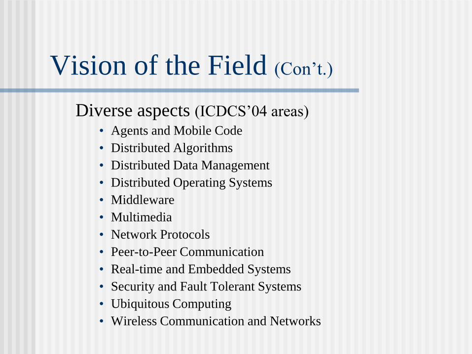
Vision of the Field (Con’t.)
Diverse aspects (ICDCS’04 areas)
• Agents and Mobile Code
• Distributed Algorithms
• Distributed Data Management
• Distributed Operating Systems
• Middleware
• Multimedia
• Network Protocols
• Peer-to-Peer Communication
• Real-time and Embedded Systems
• Security and Fault Tolerant Systems
• Ubiquitous Computing
• Wireless Communication and Networks
The Future of Distributed Computing
Theoretical aspects, including global state, logical/physical clock,
synchronization, and algorithm verification.
Fault tolerance and crash recovery through software fault tolerance.
Tools (for CASE and performance measure) and languages are badly
needs.
High-performance systems that connects 105 or more processors.
Real-time distributed systems used for automated manufacturing,
remote sensing and control, and other time-critical missions.
Actual distributed systems with significantly improved fault tolerance,
resource sharing, and communications. These systems will function as
single, coherent, powerful, virtual machines providing transparent user
access to network-wide resources.

Major “old” Challenges
Transparency
Scalability
The need to meet various goals
• Real time constraints
• Fault tolerance
• Security
• Other quality/performance related objectives
Cross-field interaction

Major “New” Challenges: Others
Supernetworks: networks are faster than the computers
attached to them
Endpoints scale to bandwidth-match the network with multiple-
10Gbps lambdas
Models that simplify distributed application programming
Middleware for bandwidth-matching distributed resources
High-speed, parallel-access storage abstractions
Adaptive and peer-to-peer data access
Real-time object models enabling predictable performance
Fault tolerance and security protocols and models
Major “New” Challenges: Green
Computing
Also green IT and ICT
Sustainability
Article: Harnessing Green
IT: Principles and Practices
Government
EPA’s Energy Star program
Industry
Climate Savers Computing
Initiative
The Green Grid
Green500
Green Comm Challenge
Algorithmic efficiency
Resource allocation
Virtualization
Terminal servers (thin client)
Power management
Data center power
Operating system support
Power supply
Storage
Video card
Display
Materials recycling
Telecommuting
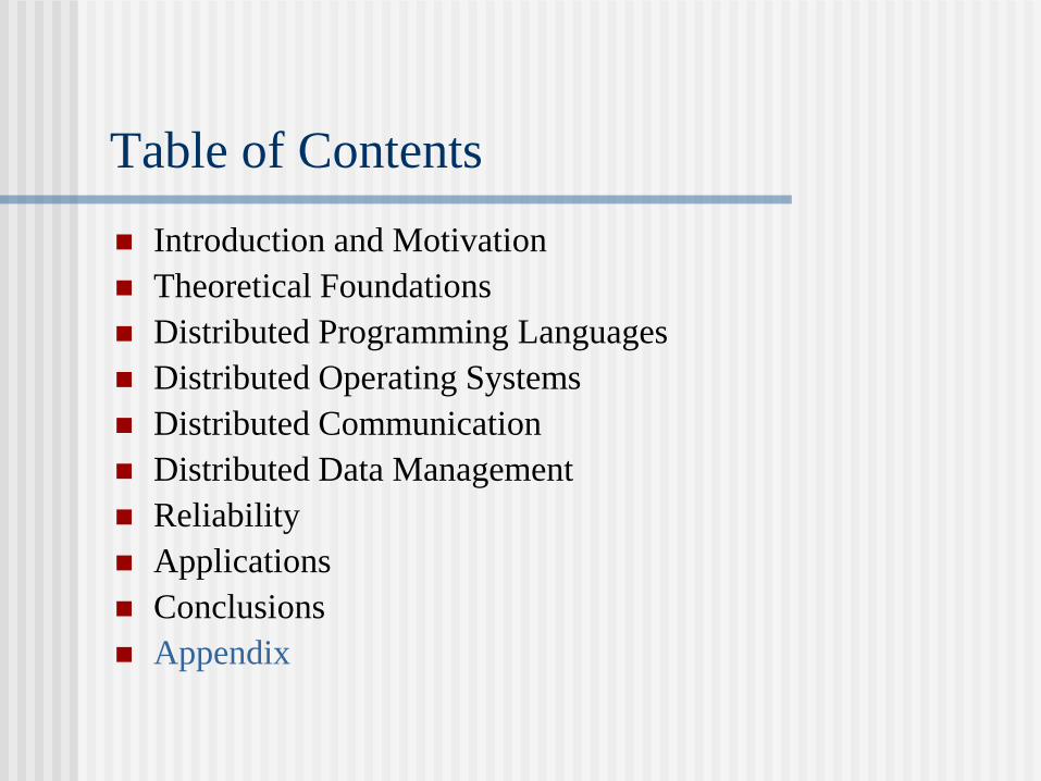
Table of Contents
Introduction and Motivation
Theoretical Foundations
Distributed Programming Languages
Distributed Operating Systems
Distributed Communication
Distributed Data Management
Reliability
Applications
Conclusions
Appendix
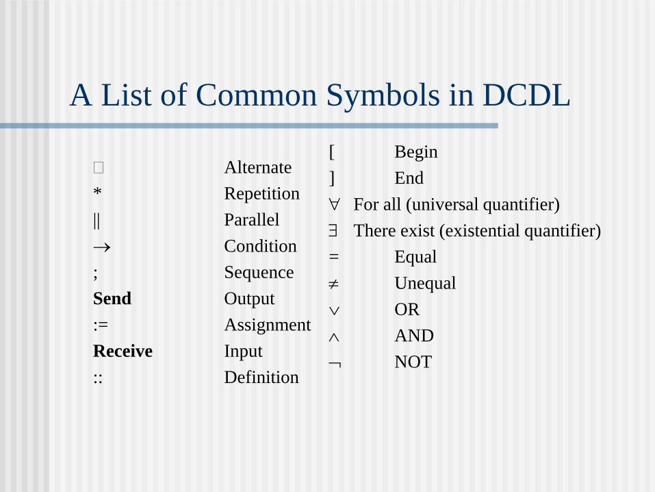
A List of Common Symbols in DCDL
Alternate
* Repetition
|| Parallel
Condition
; Sequence
Send Output
:= Assignment
Receive Input
:: Definition
[ Begin
] End
For all (universal quantifier)
There exist (existential quantifier)
= Equal
Unequal
OR
AND
NOT
Ideas for Projects
Scalability metric
Amdahl's law and Gustafson law
time-constrained
efficiency-constrained
memory-constrained scaling
Parallel/distributed environment
MPI
PVM
Parallel/distributed system model
including criteria to access their suitability.
Networks of workstations
with applications
Distributed simulation
Petri nets and other related models

Ideas for Projects (Cont’d)
Mobile computing
Routing
Checkpointing
channel allocation
Information model
switch-based LANS
internet
Routing
Optimal
fault tolerant
deadlock-free.
Scheduling
static and dynamic load distribution.
Ideas for Projects (Cont’d)
Fault tolerance
various applications
Scalable design
interconnection networks.
Survey
Database, file, DSM, heterogeneous computing, OS, etc.
Collective communication
multicast, broadcast, barrier sync., etc.
RPC and remote message passing
different approaches.
Consistency models and applications
different weak consistency models.