1

Distributed online convex optimizationover jointly connected digraphs

David Mateos-Nunez Jorge Cortes

Abstract—This paper considers networked online convex opti-mization scenarios from a regret analysis perspective. At eachround, each agent in the network commits to a decision andincurs in a local cost given by functions that are revealed overtime and whose unknown evolution model might be adversariallyadaptive to the agent’s behavior. The goal of each agent is toincur a cumulative cost over time with respect to the sum oflocal functions across the network that is competitive with thebest single centralized decision in hindsight. To achieve this,agents cooperate with each other using local averaging over time-varying weight-balanced digraphs as well as subgradient descenton the local cost functions revealed in the previous round. Wepropose a class of coordination algorithms that generalize dis-tributed online subgradient descent and saddle-point dynamics,allowing proportional-integral (and higher-order) feedback onthe disagreement among neighboring agents. We show that ouralgorithm design achieves logarithmic agent regret (when localobjectives are strongly convex), or square-root agent regret (whenlocal objectives are convex) in scenarios where the communicationgraphs are jointly connected. Simulations in a medical diagnosisapplication illustrate our results.

Index Terms—distributed optimization; online optimization; re-gret analysis; jointly connected digraphs.

I. INTRODUCTION

Networked multi-agent systems are being increasingly de-ployed in scenarios where information is dynamic and increas-ingly revealed over time. Given the limited resources availableto the network combined with the automatic and distributeddata-collection, such scenarios bring to the forefront the needfor optimizing network behavior in a distributed fashion and inreal time. Motivated by these observations, we consider herea group of N agents seeking to solve a sequential decisionproblem over a time horizon T defined by the objective

T∑

t=1

N∑

i=1

f it (x),

where each component function f it : Rd → R becomesavailable to agent i ∈ {1, . . . , N}, and only to it, after havingmade its decision at time t ∈ {1, . . . , T}. Such networkedonline optimization problems arise in regression, classification,and other estimation problems in machine learning, where thefunctions {f it} measure the fitness of some model parameters,represented by the global decision vector x ∈ Rd, with

A preliminary version of this work appeared at the 2014 InternationalSymposium on Mathematical Theory of Networks and Systems. This workwas supported by NSF Award CMMI-1300272.

The authors are with the Department of Mechanical andAerospace Engineering, University of California, San Diego,{dmateosn,cortes}@ucsd.edu.

respect to data sets that are incrementally revealed over timeand become available in a distributed way (like in sensornetworks or label-feedback systems). These problems naturallylend themselves to distributed algorithmic solutions becausethe information is distributed across the agents and makingit centrally available might be costly (e.g., communicationoverhead, latency, and message drops), undesirable (e.g., pri-vacy and security considerations), or poorly scalable (e.g.,data sets which are large and change with time). In thesescenarios, each agent would like to compute a provisionalestimate of the global optimizer without waiting until allthe data has been collected over time across the network.This represents a departure from standard static distributedoptimization problems to a distributed online optimizationframework that accounts for the adverse scenario of localdecisions being evaluated against information available to theagents only after the decisions have been made.As an example application, consider a network of hospitalsthat gather data over time about patients that might need somespecific medical procedure. Each hospital has to assess theadequacy of the procedure upon prior observations and localcommunication with neighboring hospitals in the group. Ateach time instant, the estimated parameters of the predictingmodel governing the decisions of each hospital are evaluatedagainst all the data most recently made available to thenetwork, while each piece of this newly collected data is usedlocally by each hospital to improve its model to inform futuredecisions. In abstract terms, the goal is that each agent of thenetwork performs in temporal average nearly as well as thebest decision computed in hindsight had all patient data beencentrally available. This notion is called agent regret and it is aperformance measure for algorithm design and analysis in theframework just described of distributed online optimization.Literature review: Distributed optimization problems are per-vasive in distributed and parallel computation [1], [2], and dis-tributed convex optimization constitutes a rich subfamily withmany applications to multi-agent systems. This has motivateda growing body of work, see e.g., [3], [4], [5], [6], [7], [8],on the synthesis of distributed algorithms with asymptotic con-vergence guarantees to solve a variety of networked problems,including data fusion, network formation, and resource alloca-tion. Our work here generalizes a family of distributed saddle-point subgradient algorithms [9], [7] that enjoy asymptoticconvergence with constant stepsizes and robust asymptoticbehavior in the presence of noise [10]. Online learning, onthe other hand, performs sequential decision making givenhistorical observations on the loss incurred by previous deci-

2

sions, even when the loss functions are adversarially adaptiveto the behavior of the decision maker. Interestingly, in onlineconvex optimization [11], [12], [13], [14], it is doable to becompetitive with the best single decision in hindsight. Theseworks show how the regret, i.e., the difference between thecumulative cost over time and the cost of the best single deci-sion in hindsight, is sublinear in the time horizon. Online con-vex optimization has applications to information theory [12],game theory [15], supervised online machine learning [13],online advertisement placement, and portfolio selection [14].Algorithmic approaches include online gradient descent [11],online Newton step [16], follow-the-approximate-leader [16],and online alternating directions [17]. A few recent workshave explored the combination of distributed and online con-vex optimization. The work [18] proposes distributed onlinestrategies that rely on the computation and maintenance ofspanning trees for global vector-sum operations and workunder suitable statistical assumptions on the sequence of ob-jectives. [19] studies decentralized online convex programmingfor groups of agents whose interaction topology is a chain.The works [20], [21] study agent regret without any statisticalassumptions on the sequence of objectives. [20] introducesdistributed online projected subgradient descent and showssquare-root regret (for convex cost functions) and logarithmicregret (for strongly convex cost functions). However, theanalysis critically relies on a projection step onto a compactset at each time step (which automatically guarantees theuniform boundedness of the estimates), and therefore excludesthe unconstrained case (given the non-compactness of thewhole state space). In contrast, [21] introduces distributedonline dual averaging and shows square-root regret (for convexcost functions) using a general regularized projection thatadmits both unconstrained and constrained optimization, butthe logarithmic bound is not established. Both works onlyconsider static and strongly-connected interaction digraphs.Statement of contributions: We consider a network of agentsthat communicate over a jointly connected sequence of time-dependent, weight-balanced digraphs. This means that thesuccessive unions of consecutive digraphs over periods oftime of a given length are strongly connected. The networkis involved in an online unconstrained convex optimizationscenario where no model is assumed about the evolution ofthe local objectives available to the agents. We propose a classof distributed coordination algorithms and study the associatedagent regret in the optimization of the sum of the local costfunctions across the network. Our algorithm design combinessubgradient descent on the local objectives revealed in theprevious round and proportional-integral (and/or higher-order)distributed feedback on the disagreement among neighboringagents. Assuming bounded subgradients of the local cost func-tions, we establish logarithmic agent regret bounds under localstrong convexity and square-root agent regret under convexityplus a mild geometric condition. We also characterize thedependence of the regret bounds on the network parameters.Our technical approach uses the concept of network regret,that captures the performance of the sequence of collectiveestimates across the group of agents. The derivation of the

sublinear regret bounds results from three main steps: thestudy of the difference between network and agent regret; theanalysis of the cumulative disagreement of the online estimatesvia the input-to-state stability property of a generalized Lapla-cian consensus dynamics; and the uniform boundedness of theonline estimates (and auxiliary variables) when the set of localoptimizers is uniformly bounded. With respect to previouswork, the contributions advance the current state of the artbecause of the consideration of unconstrained formulations ofthe online optimization problem, which makes the discussionvalid for regression and classification and raises major techni-cal challenges to ensure the uniform boundedness of estimates;the synthesis of a novel family of coordination algorithms thatgeneralize distributed online subgradient descent and saddle-point dynamics; and the development of regret guaranteesunder jointly connected interaction digraphs. Our novel anal-ysis framework modularizes the main technical ingredients(the disagreement evolution via linear decoupling and input-to-state stability; the boundedness of estimates and auxiliarystates through marginalizing the role of disagreement andlearning rates; and the role played by network topology andthe convexity properties) and extends and integrate techniquesfrom distributed optimization (e.g., Lyapunov techniques forconsensus under joint connectivity) and online optimization(e.g., Doubling Trick bounding techniques for square-root re-gret). We illustrate our results in a medical diagnosis example.

II. PRELIMINARIES

Here we introduce notational conventions and basic notions.Linear algebra: We denote by Rn the n-dimensional Eu-clidean space, by In ∈ Rn×n the identity matrix, and by1n ∈ Rn the column vector of all ones. For simplicity,we often use (v1, . . . , vN ) to represent the column vector[v>1 , . . . , v

>N ]>. We denote by ‖.‖2 the Euclidean norm and

by B(x, ε) := {y ∈ Rn : ‖y− x‖2 < ε} and B(x, ε) the openand closed balls, respectively, centered at x of radius ε. Givenw ∈ Rn \ {0} and c ∈ [0, 1], we let

Fc(w) :={v ∈ Rn : v>w ≥ c ‖v‖2‖w‖2

}

denote the convex cone of vectors in Rn whose angle withw has a cosine lower bounded by c. A matrix A ∈ Rn×nis diagonalizable if it can be written as A = SADAS

−1A ,

where DA ∈ Rn×n is a diagonal matrix (whose entries arethe eigenvalues of A), and SA ∈ Rn×n is an invertiblematrix (whose columns are the corresponding eigenvectors).If the eigenvalues of A are real, we label them in increasingorder from the minimum to the maximum as λmin(A) =λ1(A), . . . , λn(A) = λmax(A). For B ∈ Rn×m, we use‖B‖2 := σmax(B) for the largest singular value of B andκ(B) := ‖B‖2‖B−1‖2 = σmax(B)/σmin(B) for the conditionnumber of B. The Kronecker product of B ∈ Rn×m andC ∈ Rp×q is denoted by B ⊗ C ∈ Rnp×mq .Convex functions: Given a convex set C ⊆ Rn, a function f :C → R is convex if f(αx+(1−α)y) ≤ αf(x)+(1−α)f(y) forall α ∈ [0, 1] and x, y ∈ C. A vector ξx ∈ Rn is a subgradientof f at x ∈ C if f(y) − f(x) ≥ ξ>x (y − x), for all y ∈ C.We denote by ∂f(x) the set of all such subgradients. The

3

characterization in [22, Lemma 3.1.6] asserts that a functionf : C → R is convex if and only if ∂f(x) is nonempty foreach x ∈ C. Equivalently, f is convex if ∂f(x) is nonemptyand for each x ∈ C and ξx ∈ ∂f(x),

f(y)− f(x) ≥ ξ>x (y − x) + p(x,y)2 ‖y − x‖22,

for all y ∈ C, where p : C×C → R≥0 is the modulus of strongconvexity (whose value may be 0). For p > 0, a function fis p-strongly convex on C if p(x, y) = p for all x, y ∈ C.Equivalently, f is p-strongly convex on C if

(ξy − ξx)>(y − x) ≥ p‖y − x‖22,for each ξx ∈ ∂f(x), ξy ∈ ∂f(y), for all x, y ∈ C. Forconvenience, we denote by argmin(f) the set of minimizersof a convex function f in its domain. For β ∈ [0, 1], a convexfunction f : Rn → R with argmin(f) 6= ∅ is β-centralon Z ⊆ Rn \ argmin(f) if for each x ∈ Z , there existsy ∈ argmin(f) such that −∂f(x) ⊂ Fβ(y − x), i.e.,

−ξ>x (y − x) ≥ β ‖ξx‖2‖y − x‖2,for all ξx ∈ ∂f(x). Note that any convex function f : Rn → Rwith a nonempty set of minimizers is at least 0-central onRn \ argmin(f). Finally, a convex function f has H-boundedsubgradient sets if there exists H ∈ R>0 such that ‖ξx‖2 ≤ Hfor all ξx ∈ ∂f(x) and x ∈ Rn.Graph theory: We review basic notions from graph theoryfollowing [23]. A (weighted) digraph G := (I, E ,A) is atriplet where I := {1, . . . , N} is the vertex set, E ⊆ I × Iis the edge set, and A ∈ RN×N≥ 0

is the weighted adjacencymatrix with the property that aij := Aij > 0 if and onlyif (i, j) ∈ E . The complete graph is the digraph with edgeset I × I. Given G1 = (I, E1,A1) and G2 = (I, E2,A2), theirunion is the digraph G1∪G2 = (I, E1∪E2,A1 +A2). A path isan ordered sequence of vertices such that any pair of verticesappearing consecutively is an edge. A digraph is stronglyconnected if there is a path between any pair of distinctvertices. A sequence of digraphs

{Gt := (I, Et,At)

}t≥1

isδ-nondegenerate, for δ ∈ R>0, if the weights are uniformlybounded away from zero by δ whenever positive, i.e., foreach t ∈ Z≥1, aij,t := (At)ij > δ whenever aij,t > 0. Asequence {Gt}t≥1 is B-jointly connected, for B ∈ Z≥1, iffor each k ∈ Z≥1, the digraph GkB ∪ · · · ∪ G(k+1)B−1 isstrongly connected. The Laplacian matrix L ∈ RN×N of adigraph G is L := diag(A1N ) − A. Note that L1N = 0.The weighted out-degree and in-degree of i ∈ I are, re-spectively, dout(i) :=

∑Nj=1 aij and din(i) :=

∑Nj=1 aji. A

digraph is weight-balanced if dout(i) = din(i) for all i ∈ I,that is, 1>NL = 0. For convenience, we let LK denote theLaplacian of the complete graph with edge weights 1/N ,i.e., LK := IN − M, where M := 1

N 1N1>N . Note that LK

is idempotent, i.e., L2K = LK. For the reader’s convenience,

Table I collects the shorthand notation combining Laplacianmatrices and Kronecker products used in the paper.

III. PROBLEM STATEMENT

This section introduces the problem of interest. We begin bydescribing the online convex optimization problem for one

M = 1N1N1

>N M = M⊗ Id

LK = IN −M LK = LK ⊗ Id LK = IK ⊗ LKLt = diag(At1N )− At Lt = Lt ⊗ Id Lt = E ⊗ Lt

TABLE I: Shorthand notation for graph matrices employedalong the paper. Here, {Gt}t≥1, K ∈ Z≥1, and E ∈ RK×K .

player and then present the networked version, which is thefocus of the paper. In online convex optimization, given atime horizon T ∈ Z≥1, in each round t ∈ {1, . . . , T} a playerchooses a point xt ∈ Rd. After committing to this choice, aconvex cost function ft : Rd → R is revealed. Consequently,the ‘cost’ incurred by the player is ft(xt). Given the temporalsequence of objectives {ft}Tt=1, the regret of the player using{xt}Tt=1 with respect to a single choice u ∈ Rd in hindsightover a time horizon T is defined by

R(u, {ft}Tt=1) :=

T∑

t=1

ft(xt)−T∑

t=1

ft(u), (1)

i.e., the difference between the total cost incurred by the onlineestimates {xt}Tt=1 and the cost of a single hindsight decision u.A logical choice, if it exists, is the best decision over a timehorizon T had all the information been available a priori, i.e.,

u = x∗T ∈ arg minx∈Rd

T∑

t=1

ft(x).

In the case when no information is available about the evolu-tion of the functions {ft}Tt=1, one is interested in designing al-gorithms whose worst-case regret is upper bounded sublinearlyin the time horizon T with respect to any decision in hindsight.This ensures that, on average, the algorithm performs nearlyas well as the best single decision in hindsight.We now explain the distributed version of the online convexoptimization problem where the online player is replaced by anetwork of N agents, each with access to partial information.In the round t ∈ {1, . . . , T}, agent i ∈ {1, . . . , N} choosesa point xit corresponding to what it thinks the network as awhole should have chosen. After committing to this choice,the agent has access to a convex cost function f it : Rd → Rand the network cost is then given by the evaluation of

ft(x) :=

N∑

i=1

f it (x). (2)

Note that this function is not known to any of the agents andis not available at any single location. In this scenario, theregret of agent j ∈ {1, . . . , N} using {xjt}Tt=1 with respect toa single choice u in hindsight over a time horizon T is

Rj(u, {ft}Tt=1) :=

T∑

t=1

N∑

i=1

f it (xjt )−

T∑

t=1

N∑

i=1

f it (u).

The goal then is to design coordination algorithms among theagents that guarantee that the worst-case agent regret is upperbounded sublinearly in the time horizon T with respect to anydecision in hindsight. This would guarantee that each agentincurs an average cost over time with respect to the sum oflocal cost functions across the network that is nearly as lowas the cost of the best single choice had all the information

4

been centrally available a priori. Since information is nowdistributed across the network, agents must collaborate witheach other to determine their decisions for the next round.We assume that the network communication topology is time-dependent and described by a sequence of weight-balanced di-graphs {Gt}Tt=1 = {({1, . . . , N}, Et,At)}Tt=1. At each round,agents can use historical observations of locally revealed costfunctions and become aware through local communication ofthe choices made by their neighbors in the previous round.

IV. DYNAMICS FOR DISTRIBUTED ONLINE OPTIMIZATION

In this section we propose a distributed coordination algorithmto solve the networked online convex optimization problemdescribed in Section III. In each round t ∈ {1, . . . , T}, agenti ∈ {1, . . . , N} performs

xit+1 = xit+σ(a

N∑

j=1

aij,t(xjt−xit) +

N∑

j=1

aij,t(zjt−zit)

)−ηtgxi

t,

zit+1 = zit−σN∑

j=1

aij,t(xjt−xit), (3)

where gxit∈ ∂f it (x

it), the scalars σ, a ∈ R>0 are design

parameters, and ηt ∈ R>0 is the learning rate at time t.Agent i is responsible for the variables xi, zi, and sharestheir values with its neighbors according to the time-dependentdigraph Gt. Note that (3) is both consistent with the notion ofincremental access to information by individual agents andis distributed over Gt: each agent updates its estimate byfollowing a subgradient of the cost function revealed to itin the previous round while, at the same time, seeking toagree with its neighbors’ estimates. The latter is implementedthrough a second-order process that employs proportional-integral feedback on the disagreement. Our design is inspiredby and extends the distributed algorithms for distributed op-timization of a sum of convex functions studied in [9], [7].We use the term online subgradient descent algorithm withproportional-integral disagreement feedback to refer to (3).We next rewrite the dynamics in compact form. To do so, weintroduce the notation x := (x1, . . . , xN ) ∈ (Rd)N and z :=(z1, . . . , zN ) ∈ (Rd)N to denote the aggregate of the agents’online decisions and the aggregate of the agents’ auxiliaryvariables, respectively. For t ∈ {1, . . . , T}, we also define theconvex function ft : (Rd)N → R by

ft(x) :=

N∑

i=1

f it (xi). (4)

When all agents agree on the same choice, one recovers thevalue of the network cost function (2), ft(1N ⊗ x) = ft(x).With this notation in place, the algorithm (3) takes the form

[xt+1

zt+1

]=

[xtzt

]− σ

[aLt Lt−Lt 0

] [xtzt

]− ηt

[gxt

0

], (5)

where Lt := Lt ⊗ Id and gxt= (gx1

t, . . . , gxN

t) ∈ ∂ft(xt).

This compact-form representation suggests a more generalclass of distributed dynamics that includes (3) as a particular

case. For K ∈ Z≥1, let E ∈ RK×K be diagonalizable withreal positive eigenvalues, and define Lt := E ⊗ Lt. Considerthe dynamics on ((Rd)N )K defined by

vt+1 = (IKNd − σLt)vt − ηtgt, (6)

where gt ∈ ((Rd)N )K takes the form

gt := (gxt , 0, . . . , 0), (7)

and we use the decomposition v = (x,v2, . . . ,vK). Through-out the paper, our convergence results are formulated for thisdynamics because of its generality, which we discuss in thefollowing remark.Remark IV.1. (Online subgradient descent algorithmswith proportional and proportional-integral disagreementfeedback): The online subgradient descent algorithm withproportional-integral disagreement feedback (3) correspondsto the dynamics (6) with the choices K = 2 and

E =

[a 1−1 0

].

For a ∈ (2,∞), E has positive eigenvalues λmin(E) =a2 −√

(a2 )2 − 1 and λmax(E) = a2 +√

(a2 )2 − 1. Interestingly,the online subgradient descent algorithm with proportional dis-agreement feedback proposed in [20] (without the projectioncomponent onto a bounded convex set) also corresponds tothe dynamics (6) with the choices K = 1 and E = [1]. •Our forthcoming exposition presents the technical approach toestablish the properties of the distributed dynamics (6) withrespect to the agent regret defined in Section III. An informaldescription of our main results is as follows. Under mildconditions on the connectivity of the communication network,a suitable choice of σ, and the assumption that the time-dependent local cost functions have bounded subgradient setsand uniformly bounded optimizers, the following bounds hold:

Logarithmic agent regret: if each local cost function is lo-cally p-strongly convex and ηt = 1

p t , then any sequencegenerated by the dynamics (6) satisfies, for each j ∈{1, . . . , N},

Rj(u, {ft}Tt=1

)∈ O(‖u‖22 + log T ).

Square-root agent regret: if each local cost function is con-vex (plus a mild geometric assumption) and, for m =0, 1, 2, . . . , dlog2 T e, we take ηt = 1√

2min each period

of 2m rounds t = 2m, . . . , 2m+1 − 1, then any sequencegenerated by the dynamics (6) satisfies, for each j ∈{1, . . . , N},

Rj(u, {ft}Tt=1

)∈ O(‖u‖22

√T ).

In our technical approach to establish these sublinear agentregret bounds, we find it useful to consider the notion ofnetwork regret [18], [24] with respect to a single hindsightchoice u ∈ Rd over the time horizon T ,

RN (u, {ft}Tt=1) :=

T∑

t=1

ft(xt)−T∑

t=1

ft(1N ⊗ u),

5

to capture the performance of the sequence of collectiveestimates {xt}Tt=1 ⊆ (Rd)N . Our proof strategy builds onthis concept and relies on bounding the following terms:

(i) both the network regret and the difference between theagent and network regrets;

(ii) the cumulative disagreement of the collective estimates;(iii) the sequence of collective estimates uniformly in the

time horizon.

Section V presents the formal discussion for these results. Thecombination of these steps allows us in Section VI to formallyestablish the sublinear agent regret bounds outlined above.

V. REGRET ANALYSIS

This section presents the results outlined above on boundingthe agent and network regrets, the cumulative disagreementof the collective estimates, and the sequence of collectiveestimates for executions of the distributed dynamics (6). Theseresults are instrumental later in the derivation of the sublinearagent regret bounds, but are also of independent interest.

A. Bounds on network and agent regret

Our first result relates the agent and network regrets for anysequence of collective estimates (regardless of the algorithmthat generates them) in terms of their cumulative disagreement.Lemma V.1. (Bound on the difference between agent andnetwork regret): For T ∈ Z≥1, let {f1

t , . . . , fNt }Tt=1 be

convex functions on Rd with H-bounded subgradient sets.Then, any sequence {xt}Tt=1 ⊂ (Rd)N satisfies, for anyj ∈ {1, . . . , N} and u ∈ Rd,

Rj(u, {ft}Tt=1) ≤ RN (u, {ft}Tt=1) +NH

T∑

t=1

‖LKxt‖2,

where LK := LK ⊗ Id.

Proof: Since ft(1N⊗x) = ft(x) for all x ∈ Rd, we have

Rj(u, {ft}Tt=1)−RN (u, {ft}Tt=1)

=

T∑

t=1

(ft(1N ⊗ xjt )− ft(xt)

). (8)

The convexity of ft implies that, for any ξ ∈ ∂ft(1N ⊗ xjt ),

ft(1N ⊗ xjt )− ft(xt) ≤ ξ>(1N ⊗ xjt − xt)

≤‖ξ‖2‖1N ⊗ xjt − xt‖2 ≤√NH‖1N ⊗ xjt − xt‖2, (9)

where we have used the Cauchy-Schwarz inequality and thefact that the subgradient sets are H-bounded. In addition,

‖1N ⊗ xjt − xt‖22 =

N∑

i=1

‖xjt − xit‖22 (10)

≤ 1

2

N∑

j=1

N∑

i=1

‖xjt − xit‖22 = Nx>t LKxt.

The fact that L2K = LK = L>K allows us to write x>t LKxt =

‖LKxt‖22. The result now follows using (9) and (10) inconjunction with (8).

Next, we bound the network regret for executions of thecoordination algorithm (6) in terms of the learning rates andthe cumulative disagreement. The bound holds regardless ofthe connectivity of the communication network as long as thedigraph remains weight-balanced.Lemma V.2. (Bound on network regret): For T ∈ Z≥1, let{f1t , . . . , f

Nt }Tt=1 be convex functions on Rd with H-bounded

subgradient sets. Let the sequence {xt}Tt=1 be generated bythe coordination algorithm (6) over a sequence of arbitraryweight-balanced digraphs {Gt}Tt=1. Then, for any u ∈ Rd,and any sequence of learning rates {ηt}Tt=1 ⊂ R>0,

2RN(u, {ft}Tt=1

)≤

T∑

t=2

‖Mxt − u‖22(

1ηt− 1

ηt−1− pt(u,xt)

)

+ 2√NH

T∑

t=1

‖LKxt‖2 +NH2T∑

t=1

ηt + 1η1‖Mx1 − u‖22,

where M := M⊗Id, u := 1N⊗u and pt : (Rd)N×(Rd)N →R≥0 is the modulus of strong convexity of ft.

Proof: Left-multiplying the dynamics (6) by the block-diagonal matrix diag(1, 0, . . . , 0)⊗M ∈ R(Nd)K×(Nd)K , andusing MLt = 0, we obtain the following projected dynamics

Mxt+1 = Mxt − ηtMgxt. (11)

Note that this dynamics is decoupled from the dynamics ofv2t , . . .v

Kt . Subtracting u and taking the norm on both sides,

we get ‖Mxt+1 − u‖22 = ‖Mxt − u− ηtMgxt‖22, so that

‖Mxt+1 − u‖22 (12)

=‖Mxt − u‖22 + η2t ‖Mgxt

‖22 − 2ηt(Mgxt)>(Mxt − u)

=‖Mxt − u‖22 + η2t ‖Mgxt

‖22 − 2ηtg>xt

(Mxt − u),

where we have used M2 = M and Mu = u. Regarding thelast term, note that

− g>xt(Mxt − u) = −g>xt

(Mxt − xt)− g>xt(xt − u)

≤ g>xtLKxt + ft(u)− ft(xt)− pt(u,xt)

2 ‖u− xt‖22,where we have used LK = INd −M. Substituting into (12),we obtain

‖Mxt+1 − u‖22 ≤ ‖Mxt − u‖22 + η2t ‖Mgxt

‖22+ 2ηt

(g>xt

LKxt + ft(u)− ft(xt)− pt(u,xt)2 ‖u− xt‖22

),

so that, reordering terms,

2(ft(xt)− ft(u)) ≤ 1ηt

(‖Mxt − u‖22 − ‖Mxt+1 − u‖22

)

− pt(u,xt)‖xt − u‖22 + 2g>xtLKxt + ηt‖Mgxt‖22. (13)

Next, we bound each of the terms appearing in the last lineof (13). For the term pt(u,xt)‖xt − u‖22, note that

‖xt − u‖22 = ‖(M + LK)(xt − u)‖22 = ‖M(xt − u)‖22+ ‖LK(xt − u)‖22 + 2(xt − u)>MLK(xt − u)

= ‖Mxt − u‖22 + ‖LKxt‖22, (14)

where we have used MLK = 0 and Mu = u. Regarding theterm 2g>xt

LKxt, note that ‖gxt‖22 =

∑Ni=1 ‖gxi

t‖22 ≤ NH2

6

because the subgradient sets are bounded by H . Hence, usingthe Cauchy-Schwarz inequality,

g>xtLKxt ≤ ‖gxt‖2‖LKxt‖2 ≤

√NH‖LKxt‖2. (15)

Finally, regarding the term ηt‖Mgxt‖22 in (13), note that

‖Mgxt‖22 = ‖1N ⊗ 1N

N∑

i=1

gxit‖22 = N

∥∥∥ 1N

N∑

i=1

gxit

∥∥∥2

2

= 1N

d∑

l=1

( N∑

i=1

gxit

)2

l≤ 1

N

d∑

l=1

(N

N∑

i=1

(gxi

t

)2l

)

=

N∑

i=1

d∑

l=1

(gxi

t

)2l

=

N∑

i=1

‖gxit‖22 ≤ NH2, (16)

where in the first inequality we have used the inequality ofquadratic and arithmetic means [25]. The result now followsfrom summing the expression in (13) over the time horizon T ,discarding the negative terms, and using the upper boundsin (14)-(16).The combination of Lemmas V.1 and V.2 provides a boundon the agent regret in terms of the learning rates and thecumulative disagreement of the collective estimates. Thismotivates our next section.

B. Bound on cumulative disagreement

In this section we study the evolution of the disagreementamong the agents’ estimates under (6). Our analysis builds onthe input-to-state stability (ISS) properties of the linear part ofthe dynamics with respect to the agreement subspace, wherewe treat the subgradient term as a perturbation. Consequently,here we study the dynamics

vt+1 = (IKNd − σLt)vt + dt, (17)

where {dt}t≥1 ⊂ ((Rd)N )K is an arbitrary sequence ofdisturbances. Our first result shows that, for the purpose ofstudying the ISS properties of (17), the dynamics can bedecoupled into K first-order linear consensus dynamics.Lemma V.3. (Decoupling into a collection of first-orderconsensus dynamics): Given a diagonalizable matrix E ∈RK×K with real eigenvalues, let SE be the matrix of eigen-vectors in the decomposition E = SEDES

−1E , with DE =

diag(λ1(E), . . . , λK(E)). Then, under the change of variables

wt := (S−1E ⊗ INd)vt, (18)

the dynamics (17) is equivalently represented by the collectionof first-order dynamics on (Rd)N defined by

wlt+1 = (INd − σ λl(E)Lt)w

lt + elt, (19)

where l ∈ {1, . . . ,K}, wt = (w1t , . . . ,w

Kt ) ∈ ((Rd)N )K and

elt :=((S−1E ⊗ INd)dt

)l ∈ (Rd)N . (20)

Moreover, for each t ∈ Z≥1,

‖LKvt‖2 ≤ ‖SE‖2√K max

1≤l≤K‖LKwl

t‖2, (21)

where LK := IK ⊗ LK.

Proof: We start by noting that

Lt = SE DE S−1E ⊗ INd Lt INd

= (SE ⊗ INd) (DE ⊗ Lt) (SE ⊗ INd)−1,

and therefore we obtain the factorization

IKNd −σLt=(SE ⊗ INd)(IKNd −σDE ⊗ Lt)(SE ⊗ INd)−1.

Now, under the change of variables (18), the dynamics (17)takes the form

wt+1 = (IKNd − σDE ⊗ Lt)wt + (S−1E ⊗ INd)dt, (22)

which corresponds to the set of dynamics (19). Moreover,

LKvt = (IK ⊗ LK)(SE ⊗ INd)wt

= (SE ⊗ INd)(IK ⊗ LK)wt = (SE ⊗ INd)LKwt.

Hence, the sub-multiplicativity of the norm together with [26,Fact 9.12.22] for the norms of Kronecker products, yields

‖LKvt‖2 ≤ ‖SE ⊗ INd‖2‖LKwt‖2 = ‖SE‖2‖LKwt‖2

= ‖SE‖2( K∑

l=1

‖LKwlt‖22)1/2 ≤ ‖SE‖2

√K max

1≤l≤K‖LKwl

t‖2,

as claimed.In the next result, we use Lemma V.3 to bound the cumulativedisagreement of the collective estimates over time.Proposition V.4. (Input-to-state stability and cumula-tive disagreement of (17) over jointly connected weight-balanced digraphs): Let E ∈ RK×K be a diagonalizablematrix with real positive eigenvalues and {Gs}s≥1 a sequenceof B-jointly connected, δ-nondegenerate, weight-balanced di-graphs. For δ′ ∈ (0, 1), let

δ := min{δ′, (1− δ′) λmin(E) δ

λmax(E) dmax

}, (23)

where

dmax := max{dout,t(k) : k ∈ I, 1 ≤ t ≤ T

}. (24)

Then, for any choice

σ ∈[ δ

λmin(E)δ,

1− δλmax(E)dmax

], (25)

the dynamics (17) over {Gs}s≥1 is input-to-state stable withrespect to the nullspace of the matrix LK. Specifically, for anyt ∈ Z≥1 and any {ds}t−1

s=1 ⊂ ((Rd)N )K ,

‖LKvt‖2 ≤ CI‖v1‖2(

1− δ

4N2

)d t−1B e

+ CU max1≤s≤t−1

‖ds‖2, (26)

where

CI := κ(SE)√K ( 4

3 )2, CU :=CI

1−(1− δ

4N2

)1/B . (27)

And the cumulative disagreement satisfies, for T ∈ Z≥1,T∑

t=1

‖LKvt‖2 ≤ CU(‖v1‖2 +

T−1∑

t=1

‖dt‖2). (28)

7

Proof: The strategy of the proof is the following. Weuse Lemma V.3 to decouple (17) into K copies (for eacheigenvalue of E) of the same first-order linear consensusdynamics. We then analyze the convergence properties of thelatter using [27, Th. 1.2]. Finally, we bound the disagreementin the original network variables using again Lemma V.3.We start by noting that the selection of δ makes the setin (25) nonempty and consequently the selection of σ feasible.We write the dynamics (19), omitting the dependence onl ∈ {1, . . . ,K} for the sake of clarity, as

yt+1 = (INd − σLt)yt + et, (29)

where σ := σ λl(E) > 0 and et := elt. From (20), we have

‖et‖2 ≤ ‖(S−1E ⊗ INd)dt‖2 ≤ ‖S−1

E ‖2‖dt‖2, (30)

for each t ∈ Z≥1. Next, let

Pt := IN − σ Lt = σAt + IN − σDoutt, (31)

and define Φ(k, s) :=(PkPk−1 · · ·Ps+1Ps

)⊗ Id, for each

k ≥ s ≥ 1. The trajectory of (29) can then be expressed as

yt+1 = Φ(t, 1)y1 +

t−1∑

s=1

Φ(t, s+ 1)es + et,

for t ≥ 2. If we now multiply this equation by LK, take normson each side, and use the triangular inequality, we obtain

‖LKyt+1‖2 ≤ ‖LKΦ(t, 1)y1‖2 (32)

+

t−1∑

s=1

‖LKΦ(t, s+ 1)es‖2 + ‖LKet‖2

=√V (Φ(t, 1)y1) +

t−1∑

s=1

√V (Φ(t, s+ 1)es) +

√V (et),

where V : (Rd)N → R is defined by

V (y) := ‖LKy‖22 =

N∑

i=1

‖yi − (My)i‖22.

Our next step is to verify the hypotheses of [27, Th. 1.2] toconclude from [27, (1.23)] that, for every y ∈ (Rd)N andevery k ≥ s ≥ 1, the following holds,

V (Φ(k, s)y) ≤(1− δ

2N2

)dk−s+1B e−2

V (y). (33)

Consider the matrices {Pt}t≥1 defined in (31). Since thedigraphs are weight-balanced, i.e., 1>NLt = 0, we have1>NPt = 1>N , and since Lt1N = 0, it follows that Pt1N = 1N .Moreover, according to (24) and (25), for each t ∈ Z≥1,

(Pt)ii ≥ 1− σ dout,t(i) = 1− σλl(E) dout,t(i)

≥ 1− σ λmax(E)dmax ≥ δ,for every i ∈ I. On the other hand, for i 6= j, (Pt)ij =σaij,t ≥ 0 and therefore, if aij,t > 0, then the nondegeneracyof the adjacency matrices together with (25) implies that

(Pt)ij = σλl(E)aij,t ≥ σ λmin(E)δ ≥ δ.Summarizing, the matrices in the sequence {Pt}t≥1 are doublystochastic with entries uniformly bounded away from 0 by δ

whenever positive. These are the sufficient conditions in [27,Th. 1.2], along with B-joint connectivity, to guarantee that (33)holds. Plugging (33) into (32), and noting that

ρδ := 1− δ

4N2≥√

1− δ2N2 ,

because (1− x/2)2 ≥ 1− x for any x ∈ [0, 1], we get

‖LKyt+1‖2 ≤ ρd tB e−2

δ‖y1‖2 +

t∑

s=1

ρd t−sB e−2

δ‖es‖2. (34)

Here we have used that√V (y) ≤ ‖LK‖2‖y‖2 ≤ ‖y‖2

because ‖LK‖2 = 1 (as LK is symmetric and all its nonzeroeigenvalues are equal to 1). We now proceed to bound‖LKvt‖2 in terms of v1 and the inputs {dt}t≥1 of the originaldynamics (17). To do this, we rely on Lemma V.3. In fact,from (21), and using (34) for each of the K first-orderconsensus algorithms, we obtain

‖LKvt‖2 ≤ ‖SE‖2√K·

· max1≤l≤K

{ρd t−1B e−2

δ‖wl

1‖2 +

t−1∑

s=1

ρd t−1−s

B e−2

δ‖es‖2

}.

Recalling now (18), so that ‖wl1‖2 ≤ ‖w1‖2 ≤ ‖S−1

E ‖2‖v1‖2for each l ∈ {1, . . . ,K}, and using also (30), we obtain

‖LKvt‖2 ≤‖SE‖2√Kρ−2

δ

(ρd t−1B e

δ‖S−1

E ‖2‖v1‖2

+

t−1∑

s=1

ρd t−1−s

B eδ

‖S−1E ‖2‖ds‖2

), (35)

for all t ≥ 2 (and for t = 1 the inequality holds trivially).Equation (26) follows from (35) noting two facts. First,∑∞k=0 r

k = 11−r for any r ∈ (0, 1) and in particular for

r = ρ1/B

δ. Second, since δ ∈ (0, 1), we have

ρ−1

δ= 1

1−δ/(4N2)≤ 1

1−1/(4N2) = 4N2

4N2−1 ≤ 43 .

To obtain (28), we sum (35) over the time horizon T to getT∑

t=1

‖LKvt‖2 ≤κ(SE)√Kρ−2

δ

( 1

1− ρ1/B

δ

‖v1‖2

+

T∑

t=2

t−1∑

s=1

ρd t−1−s

B eδ

‖ds‖2),

and using r = ρ1/B

δfor brevity, the last sum is bounded as

T∑

t=2

t−1∑

s=1

rt−1−s‖ds‖2 =

T−1∑

s=1

T∑

t=s+1

rt−1−s‖ds‖2

T−1∑

s=1

‖ds‖2T∑

t=s+1

rt−1−s ≤ 1

1− rT−1∑

s=1

‖ds‖2.

This yields (28) and the proof is complete.The combination of the bound on the cumulative disagreementstated in Proposition V.4 with the bound on agent regret thatfollows from Lemmas V.1 and V.2 leads us to the next result.Corollary V.5. (Bound on agent regret under the dynam-ics (6) for arbitrary learning rates): For T ∈ Z≥1, let

8

{f1t , . . . , f

Nt }Tt=1 be convex functions on Rd with H-bounded

subgradient sets. Let E ∈ RK×K be a diagonalizable matrixwith real positive eigenvalues and {Gt}t≥1 a sequence of B-jointly connected, δ-nondegenerate, weight-balanced digraphs.If σ is chosen according to (25), then the agent regret associ-ated to a sequence {xt = (x1

t , . . . , xNt )}Tt=1 generated by the

coordination algorithm (6) satisfies, for any j ∈ {1, . . . , N},u ∈ Rd, and {ηt}Tt=1 ⊂ R>0, the bound

2Rj(u, {ft}Tt=1)

≤NT∑

t=2

‖ 1N

N∑

i=1

xit − u‖22(

1ηt− 1

ηt−1− pt(u,xt)

)

+ 4NHCU‖v1‖2 +NH2(4√NCU + 1)

T∑

t=1

ηt

+N

η1‖ 1N

N∑

i=1

xi1 − u‖22, (36)

where CU is given in (27) and pt : (Rd)N × (Rd)N → R≥0

is the modulus of strong convexity of ft.

Proof: From Lemmas V.1 and V.2, we can write

2Rj(u, {ft}Tt=1) (37)

≤T∑

t=2

‖Mxt − u‖22(

1ηt− 1

ηt−1− pt(u,xt)

)

+(2√NH + 2NH

) T∑

t=1

‖LKxt‖2 +NH2T∑

t=1

ηt

+ 1η1‖Mx1 − u‖22.

On the one hand, note that

‖Mxt − u‖22 =N‖ 1N

N∑

i=1

xit − u‖22. (38)

On the other hand, taking ds = −ηs(gxs, 0, . . . , 0) ∈

((Rd)N )K in (28) of Proposition V.4 and noting that ‖ds‖2 =ηs‖gxs‖2 ≤ ηs

√NH , we get

T∑

t=1

‖LKxt‖2 ≤T∑

t=1

‖LKvt‖2 ≤ CU(‖v1‖2 +

T−1∑

t=1

ηt√NH

).

We obtain the result by substituting this and (38) into (37),and using the bound 2

√NH + 2NH ≤ 4NH .

To establish the desired logarithmic and square-root regretbounds we need a suitable selection of learning rates in thebound obtained in Corollary V.5. This step is enabled by thefinal ingredient in our analysis: bounding the evolution of theonline estimates and all the auxiliary states uniformly in thetime horizon T . We tackle this next.

C. Bound on the trajectories uniform in the time horizon

Here we show that the trajectories of (6) are bounded uni-formly in the time horizon. For this, we first bound the meanof the online estimates and then use the ISS property of thedisagreement evolution studied in the previous section.

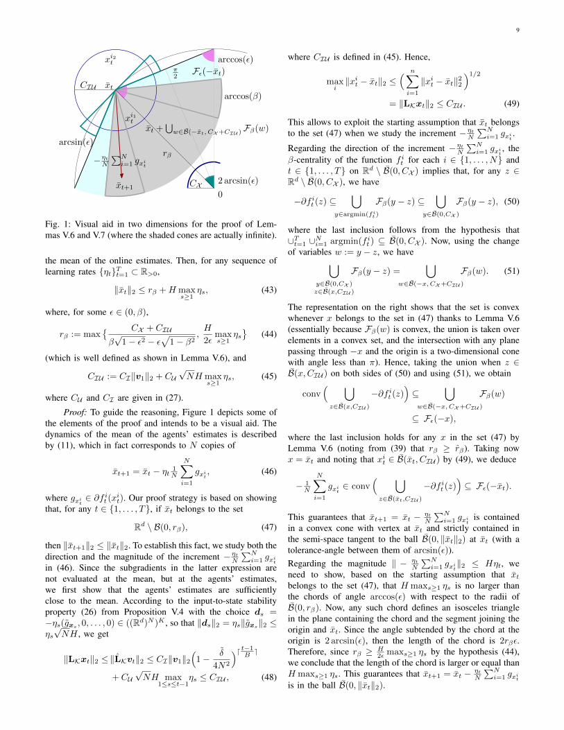
Our first result establishes a useful bound on how far fromthe origin one should be so that a certain important inclusionamong convex cones is satisfied. This plays a key role in thetechnical developments of this section.Lemma V.6. (Convex cone inclusion): Given β ∈ (0, 1],ε ∈ (0, β), and any scalars CX , CIU ∈ R>0, let

rβ :=CX + CIU

β√

1− ε2 − ε√

1− β2. (39)

Then, rβ ∈ (CX + CIU ,∞) and, for any x ∈ Rd \ B(0, rβ),⋃

w∈B(−x,CX+CIU )

Fβ(w) ⊆ Fε(−x), (40)

where the set on the left is convex.

Proof: Throughout the proof, we consider the functionsarccos and arcsin in the domain [0, 1]. Since ε ∈ (0, β) andβ ∈ (0, 1], it follows that arccos(ε) − arccos(β) ∈ (0, π/2).Now, using the angle-difference formula and noting thatsin(arccos(α)) =

√1− α2 for any α ∈ [0, 1], we have

sin(

arccos(ε)− arccos(β))

= (√

1− ε2 )β − ε√

1− β2,

which belongs to the set (0, 1) by the observation above.Therefore, rβ ∈ (CX + CIU ,∞). Let x ∈ Rd \ B(0, rβ).Since ‖x‖2 ≥ rβ > CX + CIU , then B(−x,CX + CIU ) ⊆Rd \ {0}, and the intersection of

⋃w∈B(−x,CX+CIU ) Fβ(w)

with any plane passing through the origin and −x forms atwo-dimensional cone (cf. Figure 1) with angle

2 arcsin(CX+CIU‖x‖2

)+ 2 arccos(β). (41)

In the case of the intersection of Fε(−x) with any planepassing through the origin and −x, the angle is 2 arccos(ε)(which is less than π because ε < β ≤ 1). Now, given theaxial symmetry of both cones with respect to the line passingthrough the origin and −x, (40) is satisfied if and only if

arcsin(CX+CIU‖x‖2

)+ arccos(β) ≤ arccos(ε), (42)

as implied by ‖x‖2 ≥ rβ because sin is increasing in (0, π/2).On the other hand, the inclusion (40) also guarantees that⋃w∈B(−x,CX+CIU ) Fβ(w) is a convex cone because eachFβ(w) is convex, the union is taken over elements in a convexset, and (42) implies that the angle in (41) is less than π.The following result bounds the mean of the online estimatesfor arbitrary learning rates uniformly in the time horizon.Lemma V.7. (Uniform bound on the mean of the onlineestimates): For T ∈ Z≥1, let {f1

t , . . . , fNt }Tt=1 be con-

vex functions on Rd with H-bounded subgradient sets andnonempty sets of minimizers. Let ∪Tt=1 ∪Ni=1 argmin(f it ) ⊆B(0, CX ) for some CX ∈ R>0 independent of T , and assume{f1t , . . . , f

Nt }Tt=1 are β-central on Rd \ B(0, CX ) for some

β ∈ (0, 1]. Let E ∈ RK×K be a diagonalizable matrixwith real positive eigenvalues and {Gs}s≥1 a sequence of B-jointly connected, δ-nondegenerate, weight-balanced digraphs.Let σ be chosen according to (25) and denote by {xt =(x1t , . . . , x

Nt )}Tt=1 the sequence generated by the coordination

algorithm (6). For t ∈ {1, . . . , T}, let xt := 1N

∑Ni=1 x

it denote

9

rβ

CX

CIU xt

xi1t

xi2t arccos(ε)

2 arcsin(ε)

0

π2

−ηtN∑Ni=1 gxi

t

xt+1

arccos(β)

arcsin(ε)

Fε(−xt)

xt +⋃w∈B(−xt, CX+CIU ) Fβ(w)

Fig. 1: Visual aid in two dimensions for the proof of Lem-mas V.6 and V.7 (where the shaded cones are actually infinite).

the mean of the online estimates. Then, for any sequence oflearning rates {ηt}Tt=1 ⊂ R>0,

‖xt‖2 ≤ rβ +H maxs≥1

ηs, (43)

where, for some ε ∈ (0, β),

rβ := max{ CX + CIU

β√

1− ε2 − ε√

1− β2,H

2εmaxs≥1

ηs}

(44)

(which is well defined as shown in Lemma V.6), and

CIU := CI‖v1‖2 + CU√NH max

s≥1ηs, (45)

where CU and CI are given in (27).

Proof: To guide the reasoning, Figure 1 depicts some ofthe elements of the proof and intends to be a visual aid. Thedynamics of the mean of the agents’ estimates is describedby (11), which in fact corresponds to N copies of

xt+1 = xt − ηt 1N

N∑

i=1

gxit, (46)

where gxit∈ ∂f it (xit). Our proof strategy is based on showing

that, for any t ∈ {1, . . . , T}, if xt belongs to the set

Rd \ B(0, rβ), (47)

then ‖xt+1‖2 ≤ ‖xt‖2. To establish this fact, we study both thedirection and the magnitude of the increment −ηtN

∑Ni=1 gxi

t

in (46). Since the subgradients in the latter expression arenot evaluated at the mean, but at the agents’ estimates,we first show that the agents’ estimates are sufficientlyclose to the mean. According to the input-to-state stabilityproperty (26) from Proposition V.4 with the choice ds =−ηs(gxs

, 0, . . . , 0) ∈ ((Rd)N )K , so that ‖ds‖2 = ηs‖gxs‖2 ≤

ηs√NH , we get

‖LKxt‖2 ≤‖LKvt‖2 ≤ CI‖v1‖2(

1− δ

4N2

)d t−1B e

+ CU√NH max

1≤s≤t−1ηs ≤ CIU , (48)

where CIU is defined in (45). Hence,

maxi‖xit − xt‖2 ≤

( n∑

i=1

‖xit − xt‖22)1/2

= ‖LKxt‖2 ≤ CIU . (49)

This allows to exploit the starting assumption that xt belongsto the set (47) when we study the increment −ηtN

∑Ni=1 gxi

t.

Regarding the direction of the increment −ηtN∑Ni=1 gxi

t, the

β-centrality of the function f it for each i ∈ {1, . . . , N} andt ∈ {1, . . . , T} on Rd \ B(0, CX ) implies that, for any z ∈Rd \ B(0, CX ), we have

−∂f it (z) ⊆⋃

y∈argmin(fit )

Fβ(y − z) ⊆⋃

y∈B(0,CX )

Fβ(y − z), (50)

where the last inclusion follows from the hypothesis that∪Tt=1 ∪Ni=1 argmin(f it ) ⊆ B(0, CX ). Now, using the changeof variables w := y − z, we have

⋃

y∈B(0,CX )z∈B(x,CIU )

Fβ(y − z) =⋃

w∈B(−x,CX+CIU )

Fβ(w). (51)

The representation on the right shows that the set is convexwhenever x belongs to the set in (47) thanks to Lemma V.6(essentially because Fβ(w) is convex, the union is taken overelements in a convex set, and the intersection with any planepassing through −x and the origin is a two-dimensional conewith angle less than π). Hence, taking the union when z ∈B(x,CIU ) on both sides of (50) and using (51), we obtain

conv( ⋃

z∈B(x,CIU )

−∂f it (z))⊆

⋃

w∈B(−x,CX+CIU )

Fβ(w)

⊆ Fε(−x),

where the last inclusion holds for any x in the set (47) byLemma V.6 (noting from (39) that rβ ≥ rβ). Taking nowx = xt and noting that xit ∈ B(xt, CIU ) by (49), we deduce

− 1N

N∑

i=1

gxit∈ conv

( ⋃

z∈B(xt,CIU )

−∂f it (z))⊆ Fε(−xt).

This guarantees that xt+1 = xt − ηtN

∑Ni=1 gxi

tis contained

in a convex cone with vertex at xt and strictly contained inthe semi-space tangent to the ball B(0, ‖xt‖2) at xt (with atolerance-angle between them of arcsin(ε)).Regarding the magnitude ‖ − ηt

N

∑Ni=1 gxi

t‖2 ≤ Hηt, we

need to show, based on the starting assumption that xtbelongs to the set (47), that H maxs≥1 ηs is no larger thanthe chords of angle arccos(ε) with respect to the radii ofB(0, rβ). Now, any such chord defines an isosceles trianglein the plane containing the chord and the segment joining theorigin and xt. Since the angle subtended by the chord at theorigin is 2 arcsin(ε), then the length of the chord is 2rβε.Therefore, since rβ ≥ H

2ε maxs≥1 ηs by the hypothesis (44),we conclude that the length of the chord is larger or equal thanH maxs≥1 ηs. This guarantees that xt+1 = xt − ηt

N

∑Ni=1 gxi

t

is in the ball B(0, ‖xt‖2).

10

The above argument guarantees that, if the starting assumptionthat xt belongs to the set (47) holds, then ‖xt+1‖2 ≤ ‖xt‖2.However, if the starting assumption is not true, then theprevious inequality might not hold. Since the magnitude ofthe increment in an arbitrary direction is upper bounded byH maxs≥1 ηs, adding this value to the threshold rβ in thedefinition of (47) yields the desired bound (43) for {xt}Tt=1,uniformly in T .The next result bounds the online estimates for arbitrarylearning rates in terms of the initial conditions and the uniformbound on the sets of local minimizers. The fact that the boundincludes the auxiliary states follows from the ISS property andthe invariance of the mean of the auxiliary states.Proposition V.8. (Boundedness of the online estimates andthe auxiliary states): Under the hypotheses of Lemma V.7,the trajectories of the coordination algorithm (6) are uniformlybounded in the time horizon T , for any {ηt}Tt=1 ⊂ R>0, as

‖vt‖2 ≤ C(β),

for t ∈ {1, . . . , T}, where

C(β) :=√N(rβ +H max

s≥1ηs)

+√K‖v1‖2 + CIU , (52)

and where rβ is given in (44) and CIU in (45).

Proof: We start by noting the useful decomposition vt =(IK⊗M)vt+LKvt. Using the triangular inequality, we obtain

‖vt‖2 ≤ ‖(IK ⊗M)vt‖2 + ‖LKvt‖2

≤ ‖Mxt‖2 +

K∑

l=2

‖Mvlt‖2 + ‖LKvt‖2.

The first term can be upper bounded by noting that ‖Mxt‖2 =√N‖ 1

N

∑ni=1 x

it‖2 and invoking (43) in Lemma V.7. The

second term does not actually depend on t. To see this, weuse the fact that (IK ⊗ M)(IKNd − σLt) = IK ⊗ M inthe dynamics (6) with the choice (7) to obtain the followinginvariance property of the mean of the auxiliary states,

Mvlt+1 = Mvlt = Mvl1

for l ∈ {2, . . . ,K}. Then, using the sub-multiplicativity ofthe norm and [26, Fact 9.12.22] for the norms of Kroneckerproducts in ‖M‖2 = ‖M⊗ Id‖2 = ‖M‖2‖Id‖2 = 1, we get

K∑

l=2

‖Mvl1‖2 ≤ ‖M‖2K∑

l=2

‖vl1‖2 ≤√K‖v1‖2,

where the last inequality follows from the inequality of arith-metic and quadratic means [25]. Finally, the third term is upperbounded in (48), and the result follows.The previous statements about uniform boundedness of thetrajectories can also be concluded when the objectives arestrongly convex. The following result says that local strongconvexity and bounded subgradient sets imply β-centrality.Lemma V.9. (Local strong convexity and bounded subgra-dients implies centrality away from the minimizer): Leth : Rd → R be a convex function on Rd that is also γ-strongly convex on B(y, ζ), for some γ, ζ ∈ R>0 and y ∈ Rd.

Then, for any x ∈ Rd \ B(y, ζ) and gx ∈ ∂h(x), gy ∈ ∂h(y),(gx − gy

)>(x− y) ≥ γζ ‖x− y‖2. (53)

If in addition h has H-bounded subgradient sets and 0 ∈∂h(y), then h is γζ

H -central in Rd \ B(y, ζ). (Note that if0 ∈ ∂h(y), then arg minx∈Rd h(x) = {y} is a singleton bystrong convexity in the ball B(y, ζ).)

Proof: Given any y ∈ Rd and x ∈ Rd \ B(y, ζ), letx ∈ B(y, ζ) be any point in the line segment between x andy. Consequently, for some ν ∈ (0, 1), we can write

x− y = ν(x− y) =ν

1− ν (x− x). (54)

Then, for any gx ∈ ∂h(x), gy ∈ ∂h(y), and gx ∈ ∂h(x),(gx − gy

)>(x− y) =

(gx − gx + gx − gy

)>(x− y)

=1

1− ν (gx − gx)>(x− x) +1

ν(gx − gy)>(x− y)

≥ 0 +γ

ν‖x− y‖22 = γ‖x− y‖2‖x− y‖2,

where in the inequality we have used convexity for the firstterm and strong convexity for the second term. To derive (53)we choose x satisfying ‖x − y‖2 = ζ, while the second partfollows taking gy = 0 in (53) and multiplying the right-handside by ‖gx‖2H because the latter quantity is less than 1.

VI. LOGARITHMIC AND SQUARE-ROOT AGENT REGRET

In this section, we build on our technical results of the previoussection: the general agent regret bound for arbitrary learningrates (cf. Corollary V.5), and the uniform boundedness of thetrajectories of the general dynamics (6) (cf. Proposition V.8).Equipped with these results, we are ready to select the learningrates to deduce the agent regret bounds outlined in Section IV.Our first main result establishes the logarithmic agent regretfor the general dynamics (6) under harmonic learning rates.Theorem VI.1. (Logarithmic agent regret for the dynam-ics (6)): For T ∈ Z≥1, let {f1

t , . . . , fNt }Tt=1 be convex func-

tions on Rd with H-bounded subgradient sets and nonemptysets of minimizers. Let ∪Tt=1 ∪Ni=1 argmin(f it ) ⊆ B(0, CX /2)for some CX ∈ R>0 independent of T , and assume{f1t , . . . , f

Nt }Tt=1 are p-strongly convex on B(0, C(pCX2H )),

for some p ∈ R>0, where C(·) is defined in (52). LetE ∈ RK×K be a diagonalizable matrix with real positiveeigenvalues and {Gt}t≥1 a sequence of B-jointly connected,δ-nondegenerate, weight-balanced digraphs. Let σ be chosenaccording to (25) and denote by {xt = (x1

t , . . . , xNt )}Tt=1 the

sequence generated by the coordination algorithm (6). Then,taking ηt = 1

p t , for any p ∈ (0, p ], the following regret boundholds for any j ∈ {1, . . . , N} and u ∈ Rd :

2Rj(u, {ft}Tt=1) ≤ NH2(4√NCU + 1

)

p(1 + log T )

+ 4NHCU‖v1‖2 +Np ‖ 1N

N∑

i=1

xi1 − u‖22, (55)

where CU is given by (27).

11

Proof: First we note that CX < C(pCX2H ) because rβin (44) is a lower bound for the function C(·) in (52) andCX < rβ as a consequence of Lemma V.6. Thus, the factthat each f it is p-strongly convex on B(0, C(pCX2H )) impliesthat it is also p-strongly convex on B(0, CX ). Let x∗it denotethe unique minimizer of f it . Then, argmin(f it ) ⊆ B(0, CX /2)implies that B(x∗it , CX /2) ⊆ B(0, CX ). The application ofLemma V.9 with γ = p, ζ = CX /2 and y = x∗it impliesthen that each f it is β′-central on Rd \ B(0, CX ) for anyβ′ ≤ pCX /2

H . Hence, the hypotheses of Proposition V.8 aresatisfied with β = pCX

2H and therefore the estimates satisfy thebound ‖xt‖2 ≤ ‖vt‖2 ≤ C(pCX2H ) for t ≥ 1, independentof T , which means they are confined to the region wherethe modulus of strong convexity of each f it is p. Now, themodulus of strong convexity of ft is the same as for thefunctions {f it}Ni=1. That is, for each ξy = (ξy1 , . . . , ξyN ) ∈∂ft(y) and ξx = (ξx1 , . . . , ξxN ) ∈ ∂ft(x), for all y,x ∈B(0, C(pCX2H )) ⊂ (Rd)N , one has

(ξy − ξx)>(y − x) =

N∑

i=1

(ξyi − ξxi)>(yi − xi)

≥ p

N∑

i=1

‖yi − xi‖22 = p ‖y − x‖22.

Thus, for all y, x ∈ B(0, C(pCX2H )), we can take pt(y,x) = pin (36) and hence Corollary V.5 implies the result by noting

1ηt− 1

ηt−1− pt(u,xt) = pt− p(t− 1)− p = p− p ≤ 0,

so the first sum in (36) can be bounded by 0. Finally,∑Tt=1 ηt = 1

p

∑Tt=1

1t <

1p (1 + log T ).

Our second main result establishes the square-root agent regretfor the general dynamics (6). Its proof follows from Corol-lary V.5, this time by using a bounding technique called theDoubling Trick [13, Sec. 2.3.1] in the learning rates selection.Theorem VI.2. (Square-root agent regret): For T ∈ Z≥1,let {f1

t , . . . , fNt }Tt=1 be convex functions on Rd with H-

bounded subgradient sets and nonempty sets of minimizers.Let ∪Tt=1 ∪Ni=1 argmin(f it ) ⊆ B(0, CX ) for some CX ∈ R>0

independent of T , and assume {f1t , . . . , f

Nt }Tt=1 are also β-

central on Rd \B(0, CX ) for some β ∈ (0, 1]. Let E ∈ RK×Kbe a diagonalizable matrix with real positive eigenvalues and{Gt}t≥1 a sequence of B-jointly connected, δ-nondegenerate,weight-balanced digraphs. Let σ be chosen according to (25)and denote by {xt = (x1

t , . . . , xNt )}Tt=1 the sequence gener-

ated by the coordination algorithm (6). Consider the followingchoice of learning rates called Doubling Trick scheme: form = 0, 1, 2, . . . , dlog2 T e, we take ηt = 1√

2min each period

of 2m rounds t = 2m, . . . , 2m+1 − 1. Then, the followingregret bound holds for any j ∈ {1, . . . , N} and u ∈ Rd:

2Rj(u, {ft}Tt=1) ≤√

2√2− 1

α√T , (56)

where

α :=N3/2H2CUC(β)( 4√

NH+

4

C(β)+

1√NCUC(β)

)

+N(rβ +H + ‖u‖2

)2,

where CU is given in (27) and C(·) is defined in (52).

Proof: We divide the proof in two steps. In step (i), weuse the general agent regret bound of Corollary V.5 makinga choice of constant learning rates over a fixed known timehorizon T ′. In step (ii), we use multiple times this boundtogether with the Doubling Trick [13, Sec. 2.3.1] to producean implementation procedure in which no knowledge of thetime horizon is required. Regarding (i), the choice ηt = η′ forall t ∈ {1, . . . , T ′} in (36) yields

2Rj(u, {ft}T′

t=1) ≤ 4NHCU‖v1‖2

+NH2(4√NCU + 1

)T ′η′ +

N

η′‖ 1N

N∑

i=1

xi1 − u‖22, (57)

where the first sum in (36) is upper-bounded by 0 because1η′ − 1

η′ − pt(u,xt) ≤ 0. Taking now η′ = 1/√T ′ in (57),

factoring out√T ′ and using 1 ≤

√T ′, we obtain

2Rj(u, {ft}T′

t=1) ≤(

4NHCU‖v1‖2

+NH2(4√NCU + 1

)+N‖ 1

N

N∑

i=1

xi1 − u‖22)√

T ′. (58)

This bound is of the type 2Rj(u, {ft}T′

t=1) ≤ α′√T ′, where

α′ depends on the initial conditions. This leads to step (ii).According to the Doubling Trick [13, Sec. 2.3.1], for m =0, 1, . . . dlog2 T e, the dynamics is executed in each periodof T ′ = 2m rounds t = 2m, . . . , 2m+1 − 1, where at thebeginning of each period the initial conditions are the finalvalues in the previous period. The regret bound for eachperiod is α′

√T ′ = αm

√2m, where αm is the multiplicative

constant in (58) that depends on the initial conditions in thecorresponding period. To eliminate the dependence on thelatter, by Proposition V.8, we have that ‖vt‖2 ≤ C(β), forC(·) in (52) with maxs≥1 ηs = 1. Also, using (43), we have

‖ 1N

N∑

i=1

xit − u‖2 ≤ ‖xt‖2 + ‖u‖2 ≤ rβ +H + ‖u‖2.

Since C(β) only depends on the initial conditions at thebeginning of the implementation procedure, the regret on eachperiod is now bounded as αm

√2m ≤ α

√2m, for α in the

statement. Consequently, the total regret can be bounded by

dlog2 Te∑

m=0

α√

2m = α 1−√

2dlog2 Te+1

1−√

2≤ α 1−

√2T

1−√

2≤

√2√

2−1α√T ,

which yields the desired bound.Remark VI.3. (Asymptotic dependence of logarithmicagent regret bound on network properties): Here weanalyze the asymptotic dependence of the logarithmic regretbound in Theorem VI.1 on the number of agents. It is notdifficult to see that, when N →∞, then

CUCI

=1

1− (1− δ4N2 )1/B

∼ 4N2B

δ.

12

Hence, for any B that guarantees B-joint connectivity, theasymptotic behavior as N →∞ of the bound (55) scales as

N3+1/2B

δo(T ), (59)

where limT→∞o(T )T = 0. In contrast to (59), the asymptotic

dependence on the number of agents in [20], [21], whichassume strong connectivity every time step and a doublystochastic adjacency matrix A, is

N1+1/2

1− σ2(A)o(T ), (60)

where σ2(A) is the second smallest singular value of A. (Herewe are taking into account the fact that [21] divides the regretby the number of agents.) The bounds (59) and (60) arecomparable in the case of sparse connected graphs that fail tobe good expanders (i.e., for sparse graphs with low algebraicconnectivity given by the second smallest eigenvalue of theLaplacian). This is the most reasonable comparison givenour joint-connectivity assumption. For simplicity, we examinethe case of undirected graphs because then 1 − σ2(A) =1 − λ2(A) = λ2(L), where L = diag(A1N ) − A = I − Ais the Laplacian corresponding to A. The sparsity of thegraph implies that δ, dmax ≈ 1, so that one can computethe maximum feasible δ from (23) to be δ∗ := (1 +λmax(E)dmaxλmin(E)δ )−1 ≈ (1 + λmax(E)/ λmin(E))−1. The algebraic

connectivity λ2(L) can vary even for sparse graphs. Paths andcycles are two examples of graphs that fail to be expandergraphs and their algebraic connectivity [28] is 2(1−cos(π/N))and 2(1 − cos(2π/N)), respectively (for edge-weights equalto 1), and thus proportional to 1 − cos(1/N) ∼ 1

N2 whenN →∞. With these values of δ∗ and λ2(L) (up to a constantindependent of N ), (59) and (60) become

N3+1/2B o(T ) and N3+1/2o(T ),

respectively. Expression (59) highlights the trade-offs betweenthe degree of parallelization and the regret behavior for a giventime horizon. Such trade-offs must be considered in the lightof factors like the serial processor speed and the rate of data-collection as well as the cost and bandwidth limitations oftransmitting spatially distributed data. •

VII. SIMULATION: APPLICATION TO MEDICAL DIAGNOSIS

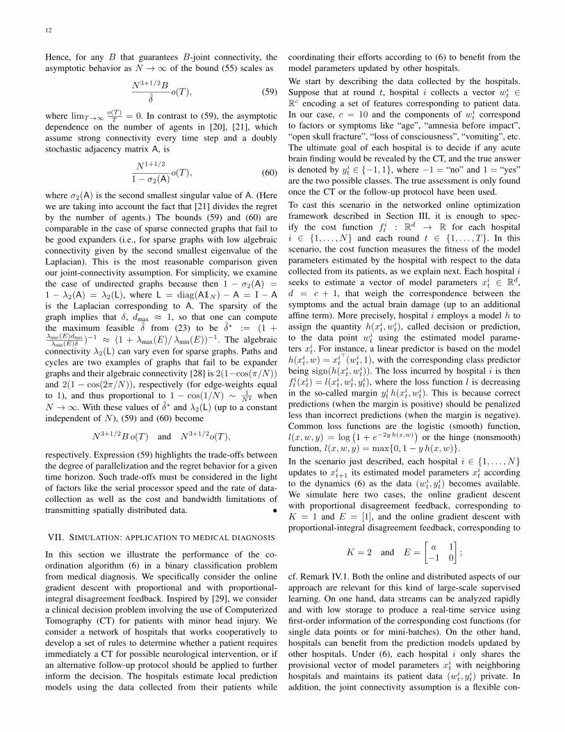
In this section we illustrate the performance of the co-ordination algorithm (6) in a binary classification problemfrom medical diagnosis. We specifically consider the onlinegradient descent with proportional and with proportional-integral disagreement feedback. Inspired by [29], we considera clinical decision problem involving the use of ComputerizedTomography (CT) for patients with minor head injury. Weconsider a network of hospitals that works cooperatively todevelop a set of rules to determine whether a patient requiresimmediately a CT for possible neurological intervention, or ifan alternative follow-up protocol should be applied to furtherinform the decision. The hospitals estimate local predictionmodels using the data collected from their patients while

coordinating their efforts according to (6) to benefit from themodel parameters updated by other hospitals.We start by describing the data collected by the hospitals.Suppose that at round t, hospital i collects a vector wit ∈Rc encoding a set of features corresponding to patient data.In our case, c = 10 and the components of wit correspondto factors or symptoms like “age”, “amnesia before impact”,“open skull fracture”, “loss of consciousness”, “vomiting”, etc.The ultimate goal of each hospital is to decide if any acutebrain finding would be revealed by the CT, and the true answeris denoted by yit ∈ {−1, 1}, where −1 = “no” and 1 = “yes”are the two possible classes. The true assessment is only foundonce the CT or the follow-up protocol have been used.To cast this scenario in the networked online optimizationframework described in Section III, it is enough to spec-ify the cost function f it : Rd → R for each hospitali ∈ {1, . . . , N} and each round t ∈ {1, . . . , T}. In thisscenario, the cost function measures the fitness of the modelparameters estimated by the hospital with respect to the datacollected from its patients, as we explain next. Each hospital iseeks to estimate a vector of model parameters xit ∈ Rd,d = c + 1, that weigh the correspondence between thesymptoms and the actual brain damage (up to an additionalaffine term). More precisely, hospital i employs a model h toassign the quantity h(xit, w

it), called decision or prediction,

to the data point wit using the estimated model parame-ters xit. For instance, a linear predictor is based on the modelh(xit, w) = xit

>(wit, 1), with the corresponding class predictor

being sign(h(xit, wit)). The loss incurred by hospital i is then

f it (xit) = l(xit, w

it, y

it), where the loss function l is decreasing

in the so-called margin yit h(xit, wit). This is because correct

predictions (when the margin is positive) should be penalizedless than incorrect predictions (when the margin is negative).Common loss functions are the logistic (smooth) function,l(x,w, y) = log

(1 + e−2y h(x,w)

)or the hinge (nonsmooth)

function, l(x,w, y) = max{0, 1− y h(x,w)}.In the scenario just described, each hospital i ∈ {1, . . . , N}updates to xit+1 its estimated model parameters xit accordingto the dynamics (6) as the data (wit, y

it) becomes available.

We simulate here two cases, the online gradient descentwith proportional disagreement feedback, corresponding toK = 1 and E = [1], and the online gradient descent withproportional-integral disagreement feedback, corresponding to

K = 2 and E =

[a 1−1 0

];

cf. Remark IV.1. Both the online and distributed aspects of ourapproach are relevant for this kind of large-scale supervisedlearning. On one hand, data streams can be analyzed rapidlyand with low storage to produce a real-time service usingfirst-order information of the corresponding cost functions (forsingle data points or for mini-batches). On the other hand,hospitals can benefit from the prediction models updated byother hospitals. Under (6), each hospital i only shares theprovisional vector of model parameters xit with neighboringhospitals and maintains its patient data (wit, y

it) private. In

addition, the joint connectivity assumption is a flexible con-

13

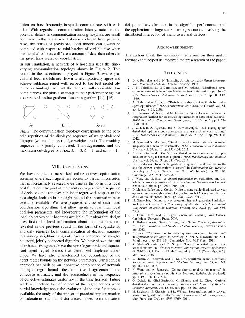
dition on how frequently hospitals communicate with eachother. With regards to communication latency, note that thepotential delays in communication among hospitals are smallcompared to the rate at which data is collected from patients.Also, the fitness of provisional local models can always becomputed with respect to mini-batches of variable size whenone hospital collects a different amount of data than others inthe given time scales of coordination.In our simulation, a network of 5 hospitals uses the time-varying communication topology shown in Figure 2. Thisresults in the executions displayed in Figure 3, where pro-visional local models are shown to asymptotically agree andachieve sublinear regret with respect to the best model ob-tained in hindsight with all the data centrally available. Forcompleteness, the plots also compare their performance againsta centralized online gradient descent algorithm [11], [16].

Gt′ Gt′+1 Gt′+2

Fig. 2: The communication topology corresponds to the peri-odic repetition of the displayed sequence of weight-balanceddigraphs (where all nonzero edge weights are 1). The resultingsequence is 3-jointly connected, 1-nondegenerate, and themaximum out-degree is 1, i.e., B = 3, δ = 1, and dmax = 1.

VIII. CONCLUSIONS

We have studied a networked online convex optimizationscenario where each agent has access to partial informationthat is increasingly revealed over time in the form of a localcost function. The goal of the agents is to generate a sequenceof decisions that achieves sublinear regret with respect to thebest single decision in hindsight had all the information beencentrally available. We have proposed a class of distributedcoordination algorithms that allow agents to fuse their localdecision parameters and incorporate the information of thelocal objectives as it becomes available. Our algorithm designuses first-order local information about the cost functionsrevealed in the previous round, in the form of subgradients,and only requires local communication of decision parame-ters among neighboring agents over a sequence of weight-balanced, jointly connected digraphs. We have shown that ourdistributed strategies achieve the same logarithmic and square-root agent regret bounds that centralized implementationsenjoy. We have also characterized the dependence of theagent regret bounds on the network parameters. Our technicalapproach has built on an innovative combination of networkand agent regret bounds, the cumulative disagreement of thecollective estimates, and the boundedness of the sequenceof collective estimates uniformly in the time horizon. Futurework will include the refinement of the regret bounds whenpartial knowledge about the evolution of the cost functions isavailable, the study of the impact of practical implementationconsiderations such as disturbances, noise, communication

delays, and asynchronism in the algorithm performance, andthe application to large-scale learning scenarios involving thedistributed interaction of many users and devices.

ACKNOWLEDGMENTS

The authors thank the anonymous reviewers for their usefulfeedback that helped us improved the presentation of the paper.

REFERENCES

[1] D. P. Bertsekas and J. N. Tsitsiklis, Parallel and Distributed Computa-tion: Numerical Methods. Athena Scientific, 1997.

[2] J. N. Tsitsiklis, D. P. Bertsekas, and M. Athans, “Distributed asyn-chronous deterministic and stochastic gradient optimization algorithms,”IEEE Transactions on Automatic Control, vol. 31, no. 9, pp. 803–812,1986.

[3] A. Nedic and A. Ozdaglar, “Distributed subgradient methods for multi-agent optimization,” IEEE Transactions on Automatic Control, vol. 54,no. 1, pp. 48–61, 2009.

[4] B. Johansson, M. Rabi, and M. Johansson, “A randomized incrementalsubgradient method for distributed optimization in networked systems,”SIAM Journal on Control and Optimization, vol. 20, no. 3, pp. 1157–1170, 2009.

[5] J. C. Duchi, A. Agarwal, and M. J. Wainwright, “Dual averaging fordistributed optimization: convergence analysis and network scaling,”IEEE Transactions on Automatic Control, vol. 57, no. 3, pp. 592–606,2012.

[6] M. Zhu and S. Martınez, “On distributed convex optimization underinequality and equality constraints,” IEEE Transactions on AutomaticControl, vol. 57, no. 1, pp. 151–164, 2012.

[7] B. Gharesifard and J. Cortes, “Distributed continuous-time convex opti-mization on weight-balanced digraphs,” IEEE Transactions on AutomaticControl, vol. 59, no. 3, pp. 781–786, 2014.

[8] D. P. Bertsekas, “Incremental gradient, subgradient, and proximal meth-ods for convex optimization: a survey,” in Optimization for MachineLearning (S. Sra, S. Nowozin, and S. J. Wright, eds.), pp. 85–120,Cambridge, MA: MIT Press, 2011.

[9] J. Wang and N. Elia, “A control perspective for centralized and dis-tributed convex optimization,” in IEEE Conf. on Decision and Control,(Orlando, Florida), pp. 3800–3805, 2011.

[10] D. Mateos-Nunez and J. Cortes, “Noise-to-state stable distributed convexoptimization on weight-balanced digraphs,” in IEEE Conf. on Decisionand Control, (Florence, Italy), pp. 2781–2786, 2013.

[11] M. Zinkevich, “Online convex programming and generalized infinites-imal gradient ascent,” in Proceedings of the Twentieth InternationalConference on Machine Learning, (Washighton, D.C.), pp. 928–936,2003.

[12] N. Cesa-Bianchi and G. Lugosi, Prediction, Learning, and Games.Cambridge University Press, 2006.

[13] S. Shalev-Shwartz, Online Learning and Online Convex Optimization,vol. 12 of Foundations and Trends in Machine Learning. Now PublishersInc, 2012.

[14] E. Hazan, “The convex optimization approach to regret minimization,”in Optimization for Machine Learning (S. Sra, S. Nowozin, and S. J.Wright, eds.), pp. 287–304, Cambridge, MA: MIT Press, 2011.

[15] S. Shalev-Shwartz and Y. Singer, “Convex repeated games andfenchel duality,” in Advances in Neural Information Processing Systems(B. Scholkopf, J. Platt, and T. Hoffman, eds.), vol. 19, (Cambridge, MA),MIT Press, 2007.

[16] E. Hazan, A. Agarwal, and S. Kale, “Logarithmic regret algorithmsfor online convex optimization,” Machine Learning, vol. 69, no. 2-3,pp. 169–192, 2007.

[17] H. Wang and A. Banerjee, “Online alternating direction method,” inInternational Conference on Machine Learning, (Edinburgh, Scotland),pp. 1119–1126, July 2012.

[18] O. Dekel, R. Gilad-Bachrach, O. Shamir, and L. Xiao, “Optimaldistributed online prediction using mini-batches,” Journal of MachineLearning Research, vol. 13, no. Jan, pp. 165–202, 2012.

[19] M. Raginsky, N. Kiarashi, and R. Willett, “Decentralized online convexprogramming with local information,” in American Control Conference,(San Francisco, CA), pp. 5363–5369, 2011.

14

0 50 100 150 200 250 300−0.5

0

0.5

1

{ xit ,7}Ni=1

Centralized

0 50 100 150 200 250 300−0.5

0

0.5

1

time, t

{ xit ,8}Ni=1

(a) Agents’ estimates using proportional-integral disagreement feedback

0 50 100 150 200 250 300

100

time horizon, T

maxj 1/T Rj(x∗T ,

{ ∑Ni f i

t

}T

t=1

)

Proport ional-Integraldisagreement feedback

Proport ionaldisagreement feedback

Centralized

(b) Average regret

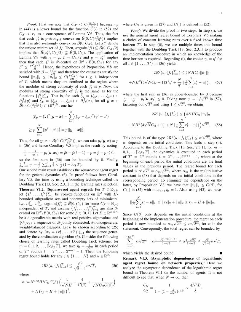
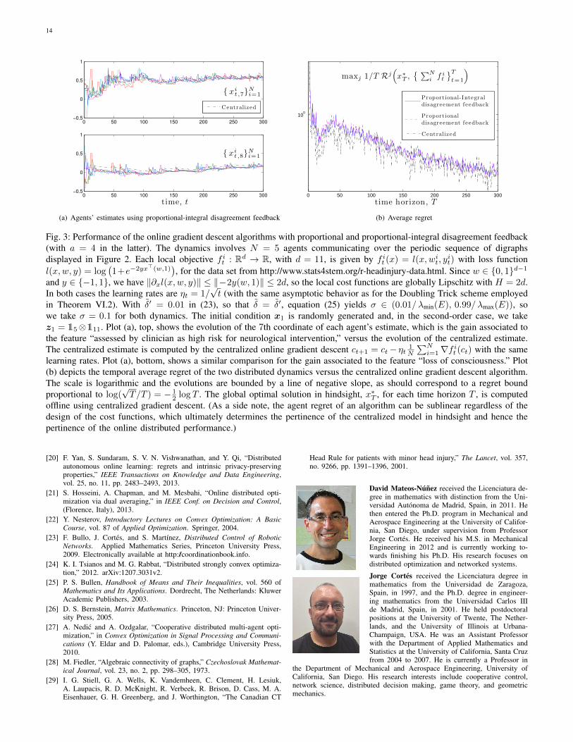
Fig. 3: Performance of the online gradient descent algorithms with proportional and proportional-integral disagreement feedback(with a = 4 in the latter). The dynamics involves N = 5 agents communicating over the periodic sequence of digraphsdisplayed in Figure 2. Each local objective f it : Rd → R, with d = 11, is given by f it (x) = l(x,wit, y

it) with loss function

l(x,w, y) = log(1+e−2yx>(w,1)

), for the data set from http://www.stats4stem.org/r-headinjury-data.html. Since w ∈ {0, 1}d−1

and y ∈ {−1, 1}, we have ‖∂xl(x,w, y)‖ ≤ ‖−2y(w, 1)‖ ≤ 2d, so the local cost functions are globally Lipschitz with H = 2d.In both cases the learning rates are ηt = 1/

√t (with the same asymptotic behavior as for the Doubling Trick scheme employed

in Theorem VI.2). With δ′ = 0.01 in (23), so that δ = δ′, equation (25) yields σ ∈ (0.01/ λmin(E), 0.99/ λmax(E)), sowe take σ = 0.1 for both dynamics. The initial condition x1 is randomly generated and, in the second-order case, we takez1 = 15⊗111. Plot (a), top, shows the evolution of the 7th coordinate of each agent’s estimate, which is the gain associated tothe feature “assessed by clinician as high risk for neurological intervention,” versus the evolution of the centralized estimate.The centralized estimate is computed by the centralized online gradient descent ct+1 = ct− ηt 1

N

∑Ni=1∇f it (ct) with the same

learning rates. Plot (a), bottom, shows a similar comparison for the gain associated to the feature “loss of consciousness.” Plot(b) depicts the temporal average regret of the two distributed dynamics versus the centralized online gradient descent algorithm.The scale is logarithmic and the evolutions are bounded by a line of negative slope, as should correspond to a regret boundproportional to log(

√T/T ) = − 1

2 log T . The global optimal solution in hindsight, x∗T , for each time horizon T , is computedoffline using centralized gradient descent. (As a side note, the agent regret of an algorithm can be sublinear regardless of thedesign of the cost functions, which ultimately determines the pertinence of the centralized model in hindsight and hence thepertinence of the online distributed performance.)

[20] F. Yan, S. Sundaram, S. V. N. Vishwanathan, and Y. Qi, “Distributedautonomous online learning: regrets and intrinsic privacy-preservingproperties,” IEEE Transactions on Knowledge and Data Engineering,vol. 25, no. 11, pp. 2483–2493, 2013.

[21] S. Hosseini, A. Chapman, and M. Mesbahi, “Online distributed opti-mization via dual averaging,” in IEEE Conf. on Decision and Control,(Florence, Italy), 2013.

[22] Y. Nesterov, Introductory Lectures on Convex Optimization: A BasicCourse, vol. 87 of Applied Optimization. Springer, 2004.

[23] F. Bullo, J. Cortes, and S. Martınez, Distributed Control of RoboticNetworks. Applied Mathematics Series, Princeton University Press,2009. Electronically available at http://coordinationbook.info.

[24] K. I. Tsianos and M. G. Rabbat, “Distributed strongly convex optimiza-tion,” 2012. arXiv:1207.3031v2.

[25] P. S. Bullen, Handbook of Means and Their Inequalities, vol. 560 ofMathematics and Its Applications. Dordrecht, The Netherlands: KluwerAcademic Publishers, 2003.

[26] D. S. Bernstein, Matrix Mathematics. Princeton, NJ: Princeton Univer-sity Press, 2005.

[27] A. Nedic and A. Ozdgalar, “Cooperative distributed multi-agent opti-mization,” in Convex Optimization in Signal Processing and Communi-cations (Y. Eldar and D. Palomar, eds.), Cambridge University Press,2010.

[28] M. Fiedler, “Algebraic connectivity of graphs,” Czechoslovak Mathemat-ical Journal, vol. 23, no. 2, pp. 298–305, 1973.

[29] I. G. Stiell, G. A. Wells, K. Vandemheen, C. Clement, H. Lesiuk,A. Laupacis, R. D. McKnight, R. Verbeek, R. Brison, D. Cass, M. A.Eisenhauer, G. H. Greenberg, and J. Worthington, “The Canadian CT

Head Rule for patients with minor head injury,” The Lancet, vol. 357,no. 9266, pp. 1391–1396, 2001.

David Mateos-Nunez received the Licenciatura de-gree in mathematics with distinction from the Uni-versidad Autonoma de Madrid, Spain, in 2011. Hethen entered the Ph.D. program in Mechanical andAerospace Engineering at the University of Califor-nia, San Diego, under supervision from ProfessorJorge Cortes. He received his M.S. in MechanicalEngineering in 2012 and is currently working to-wards finishing his Ph.D. His research focuses ondistributed optimization and networked systems.

Jorge Cortes received the Licenciatura degree inmathematics from the Universidad de Zaragoza,Spain, in 1997, and the Ph.D. degree in engineer-ing mathematics from the Universidad Carlos IIIde Madrid, Spain, in 2001. He held postdoctoralpositions at the University of Twente, The Nether-lands, and the University of Illinois at Urbana-Champaign, USA. He was an Assistant Professorwith the Department of Applied Mathematics andStatistics at the University of California, Santa Cruzfrom 2004 to 2007. He is currently a Professor in

the Department of Mechanical and Aerospace Engineering, University ofCalifornia, San Diego. His research interests include cooperative control,network science, distributed decision making, game theory, and geometricmechanics.