Embed Size (px)
Citation preview

DISTRIBUTED GENERATION ALLOCATION FOR POWER LOSS MINIMIZATION AND VOLTAGE IMPROVEMENT OF RADIAL DISTRIBUTION
SYSTEMS USING GENETIC ALGORITHM
By
DIPANJAN SAMAJPATI
DEPARTMENT OF ELECTRICAL ENGINEERING
NATIONAL INSTITUTE OF TECHNOLOGY, ROURKELA
ROURKELA-769008
© Copyright by Dipanjan Samajpati, 2014

DISTRIBUTED GENERATION ALLOCATION FOR POWER LOSS MINIMIZATION AND VOLTAGE IMPROVEMENT OF
RADIAL DISTRIBUTION SYSTEMS USING GENETIC ALGORITHM
A Thesis for the award of the degree of
Master of Technology In
Electrical Engineering
NIT Rourkela
Submitted By:
Dipanjan Samajpati (Roll no.: 212EE4253)
Under the esteemed guidance of Dr. Sanjib Ganguly
Assistant Professor, EED
May, 2014
DEPARMENT OF ELECTRICAL ENGINEERING NATIONAL INSTITUTE OF TECHNOLOGY, ROURKELA
ROURKELA-769008

NIT Rourkela
CERTIFICATE
I hereby certify that the work which is being presented in the thesis
entitled “Distributed Generation Allocation For Power Loss
Minimization And Voltage Improvement Of Radial Distribution
Systems Using Genetic Algorithm” in partial fulfilment of the
requirements for the award of Master Of Technology degree in
Electrical Engineering submitted in Electrical Engineering
Department of National Institute of Technology, Rourkela is an
authentic record of my own work carried out under the supervision
of Dr. Sanjib Ganguly, Assistant Professor, Department of Electrical
Engineering.
The matter presented in this thesis has not been submitted for the
award of any other degree of this or any other university.
(Dipanjan Samajpati)
This is certify that the above statement made by candidate is correct
and true to best of my knowledge.
(Dr. Sanjib Ganguly)
Department of Electrical Engineering National Institute of Technology, Rourkela
Rourkela -769008

This thesis is dedicated
To the soul of my Father and beloved Mother, May God bless them and elongate them live in his
obedience!!
To my best friend Smarani, May God bless her and give her a sweet, happy, deserving
trustful life!!
---Dipanjan Samajpati

ACKNOWLEDGMENTS
First and foremost, I am deeply obligated to Dr. Sanjib Ganguly my advisor and guide, for
the motivation, guidance, tutelage and patience throughout the research work. I appreciate his
broad range of expertise and attention to detail, as well as the constant encouragement he has
given me over the years. There is no need to mention that a big part of this thesis is the result
of joint work with him, without which the completion of the work would have been impossible.
Last but not least, I would like to express my deep thanks to my family and one of my best
friend for their unlimited support and encouragement. Their pray and love was my source and
motivation to continue and finish this research.
Dipanjan Samajpati

ABSTRACT
Numerous advantages attained by integrating Distributed Generation (DG) in distribution
systems. These advantages include decreasing power losses and improving voltage profiles.
Such benefits can be achieved and enhanced if DGs are optimally sized and located in the
systems. This theses presents a distribution generation (DG) allocation strategy to improve
node voltage and power loss of radial distribution systems using genetic algorithm (GA). The
objective is to minimize active power losses while keep the voltage profiles in the network
within specified limit. In this thesis, the optimal DG placement and sizing problem is
investigated using two approaches. First, the optimization problem is treated as single-objective
optimization problem, where the system’s active power losses are considered as the objective
to be minimized. Secondly, the problem is tackled as a multi-objective one, focusing on total
power loss as well as voltage profile of the networks. This approach finds optimal DG active
power and optimal OLTC position for tap changing transformer. Also uncertainty in load and
generation are considered. Thus, in this work, the load demand at each node and the DG power
generation at candidate nodes are considered as a possibilistic variable represented by two
different triangular fuzzy number. A 69-node radial distribution system and 52-node practical
radial systems are used to demonstrate the effectiveness of the proposed methods. The
simulation results shows that reduction of power loss in distribution system is possible and all
node voltages variation can be achieved within the required limit if DG are optimally placed in
the system. Induction DG placement into the distribution system also give a better performance
from capacitor bank placement. In modern load growth scenario uncertainty load and
generation model shows that reduction of power loss in distribution system is possible and all
node voltages variation can be achieved within the required limit without violating the thermal
limit of the system.

vii
TABLE OF CONTENTS
ABSTRACT
Table of Contents vii
List of Tables x
List of Figures xii
List of Abbreviations and Symbols Used xvii
CHAPTER 1 Introduction and Literature Review 1-10
1.1 Introduction 1
1.2 Objective of the Work 4
1.3 Literature Review 5
1.3.1 Distribution Networks and Distributed Generation 5
1.3.2 Uncertainty in Distribution Planning 9
1.4 Organization of the Report 10
CHAPTER 2 Modelling and Allocation of DG in Distribution
Networks
11-16
2.1 Introduction 11
2.2 Distribution Network Power Losses 12
2.3 Distributed Generation 12
2.3.1 Operational And Planning Issues With DGs 12
2.3.2 DG Operation 13
2.3.3 DG Siting 14
2.3.4 DG Sizing 14
2.4 Summary 16
CHAPTER 3 Incorporation of DG Model in Distribution System
Load Flows
17-40
3.1 Introduction 17
3.2 Load Flow of Radial Distribution Systems 18
3.2.1 Equivalent Current Injection 19
3.2.2 Formation of BIBC Matrix 19
3.2.3 Formation of BCBV Matrix 21
3.2.4 Solution Methodology 24
3.3 Algorithm for Distribution System Load Flow 26
3.4 Incorporation of DG into Load Flow 28

viii
3.5 Incorporation of OLTC into Load Flow 29
3.6 Incorporation of CB into Load Flow 30
3.7 Algorithm for Distribution System Load Flow with DG 30
3.8 Test System 32
3.9 Load Flow Solution for Base Case 35
3.10 Summary 40
CHAPTER 4 Optimal DG allocation Using Genetic Algorithm 41-96
4.1 Introduction 41
4.2 Genetic Algorithm 41
4.2.1 GAs vs Conventional Algorithms 42
4.2.2 Genetic Algorithm Description 42
4.2.3 Parameters of GA 44
4.2.4 Algorithm of Basic GA 45
4.2.5 Applications of GA 47
4.3 DG Allocation Optimization Objective Function 48
4.4 Basic-GA Optimization for DG Allocation 49
4.4.1 Coding Scheme 50
4.4.2 Initialization 50
4.4.3 Fitness Function 52
4.4.4 Reproduction 52
4.4.5 Crossover 53
4.4.6 Mutation 55
4.4.7 Elitism 56
4.4.8 Genetic Control Parameters Selection 56
4.5 Algorithm for DG Allocation 57
4.6 Case Study for Basic GA Optimization 60
4.6.1 Selection of GA Parameter for DG Allocation 61
4.6.2 Single-Objective Optimization With Basic GA - 63
Results of First Approach 63
Results of Second Approach 70
4.6.3 Multi-Objective Optimization With Basic GA 74
4.7 Improved/Adaptive Genetic Algorithm (IGA)
Optimization
78
4.7.1 Algorithm of Adaptive GA 80

ix
4.8 Case Study Adaptive Genetic Algorithm Optimization 82
4.8.1 Case Study for Adaptive GA#3 Optimization 83
4.9 Proposed Adaptive-GA Optimization 89
4.10 Case Study for Selection of Uncrossed Parents 94
4.11 Summary 96
CHAPTER 5 Optimal DG Allocation Under Variable Load and
Generation Using Genetic Algorithm
97-123
5.1 Introduction 97
5.2 Multi-Objective Planning of Radial Distribution
Networks Using PLGM
98
5.2.1 Possibilistic Load and Generation Model (PLGM) 99
5.2.2 Comparison of Fuzzy Numbers 100
5.3 Objective Functions 101
5.4 DG Allocation Strategy Using GA 102
5.5 Case Study for Uncertainty in Load and Generation 105
5.5.1 Deterministic load and generation analysis 105
5.5.2 Possibilistic load and generation analysis 108
5.5.3 Multiple run for deterministic and possibilistic load
and generation
109
5.5.4 Multiple run uncertainty analysis with different
system and GA parameter
115
5.5.5 Multiple run uncertainty analysis with different DG
rating limit
117
5.5.6 Violation of system constraint in overloading
condition
119
5.6 Summary 123
CHAPTER 6 Conclusion and Scope for Future Work 124-127
6.1 Conclusions 124
6.2 Scope for Future Work 127
REFERENCES 128-137
RESEARCH PUBLICATIONS 138
APPENDIX A 139-142

x
LIST OF TABLES
Table 3.1 Base case converged flow solution for system #1. 38
Table 3.2 Base case converged flow solution for system #2. 39
Table 4.1 GA parameter selection with system#1 62
Table 4.2 Base case converged cower flow solution for system #1. 63
Table 4.3 Comparison of various cases optimization operation 64
Table 4.4 Converged Power Flow Solution of case#1(a); case#1(a),
unity p.f. DG
67
Table 4.5 Converged Power Flow Solution of case#2(a); case#2(a),
unity p.f. DG and OLTC
68
Table 4.6 Optimal Power Flow Solutions for 10 run. 69
Table 4.7 Comparison of various cases optimization operation. 70
Table 4.8 Converged Power Flow Solution for 10 run. 73
Table 4.9 GA and network parameters considered for the optimization
process
74
Table 4.10 Multiple run solution for different case with system#2 76
Table 4.11 Multi-objective optimization for different system with basic
GA optimization
77
Table 4.12 Comparison of various GA optimization for DG allocation
with system#1
82
Table 4.13 Different case study for different system with GA#3
optimization
88
Table 4.14 Position and rating for DG and CB of GA#3 optimization in
different cases
88
Table 4.15 Different case study for different system with GA#6
optimization
93
Table 4.16 Comparison of various uncrossed parents selection approach
of GA optimization for dg allocation
94

xi
Table 5.1 Study for deterministic load of 0.6 p.u. on test systems with
Ga#6 optimization
105
Table 5.2 Study for deterministic load of 1.0 p.u. on test systems with
Ga#6 optimization
106
Table 5.3 Study for possibilistic load of 0.4 p.u to 1.4 p.u. on test
systems with Ga#6 optimization
107
Table 5.4 Study for deterministic load of 1.6 p.u. and 1.2 p.u. of base
load on test systems with Ga#6 optimization
108
Table 5.5 Effective nodes DG ratings median value for various cases 115
Table 5.6 GA and network parameters considered for the optimization
process
115
Table 5.7 Effective nodes DG ratings median value for various cases 116

xii
LIST OF FIGURES
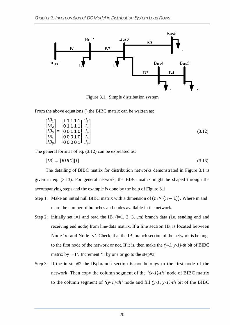
Figure 3.1 Simple distribution system. 20
Figure 3.2 The formation of BIBC matrix, the example is done by the help
of Figure 3.1.
21
Figure 3.3 The formation of BVBC matrix, the example is done by the
help of Figure 3.1.
24
Figure 3.4 Flowchart for load flow solution for radial distribution
networks.
27
Figure 3.5 Network with off-nominal tap changing transformer. 29
Figure 3.6 System #1, 69-Node Radial Distribution Networks. 33
Figure 3.7 System #2, 52-Node Radial Distribution Networks. 34
Figure 3.8 Base case node voltage magnitudes of system#1. 36
Figure 3.9 Base case branch current magnitudes of system#1. 36
Figure 3.10 Base case node voltage magnitudes of system#2. 37
Figure 3.11 Base case branch current magnitudes of system#2. 37
Figure 4.1 Flowchart for basic GA algorithms. 46
Figure 4.2 Flowchart of DG allocation with basic genetic algorithm. 59
Figure 4.3 Node voltage magnitude of system#1; case#1(a), unity p.f.
DG; case#2(a), unity p.f. DG and OLTC.
64
Figure 4.4 Branch current magnitude of system#1; case#1(a), unity p.f.
DG; case#2(a), unity p.f. DG and OLTC.
65
Figure 4.5 Generation wise variation of average and minimum power loss
of system#1 for case#1(a) unity p.f. DG.
65
Figure 4.6 Generation wise variation of average and minimum power loss
of system#1 for case#2(a) unity p.f. DG and OLTC.
66
Figure 4.7 Comparison of average and minimum power loss in different
cases; case#1(a), unity p.f. DG; case#2(a), unity p.f. DG and
OLTC.
66

xiii
Figure 4.8 Run wise variation of minimum and average power losses. 69
Figure 4.9 Node voltage magnitude of system#1; case#1(a), unity p.f.
DG; case#2(a), unity p.f. DG and OLTC.
70
Figure 4.10 Branch current magnitude of system#1; case#1(a), unity p.f.
DG; case#2(a), unity p.f. DG and OLTC.
71
Figure 4.11 Comparison of average and minimum power loss in different
cases; case#1(a), unity p.f. DG; case#2(a), unity p.f. DG and
OLTC.
71
Figure 4.12 Comparison of average and minimum objective function in
different cases; case#1(a), unity p.f. DG; case#2(a), unity p.f.
DG and OLTC.
72
Figure 4.13 Run wise variation of minimum and average power losses 73
Figure 4.14 Variation of optimal active and reactive power loss of
system#1.
74
Figure 4.15 Variation of optimal active and reactive power loss of
system#2.
75
Figure 4.16 Variation of minimum node voltage of system#1 and
system#2.
75
Figure 4.17 Variation of maximum branch current of system#1 and
system#2.
76
Figure 4.18 Flowchart of adaptive genetic algorithm for DG allocations. 81
Figure 4.19 Average objective function of different GA for System#1. 82
Figure 4.20 Convergence of GA#3 for unity p.f. DG optimization with
System#1.
83
Figure 4.21 Adaptive crossover probability of GA#3 with System#2. 84
Figure 4.22 Adaptive mutation probability of GA#3 with System#2. 84
Figure 4.23 Node voltage magnitude of GA#3 for system#1 in different
cases.
85

xiv
Figure 4.24 Active and Reactive power loss with injected DG and capacitor
bank power rating.
85
Figure 4.25 Node voltage magnitude of GA#3 for System#2 86
Figure 4.26 Node voltage magnitude of GA#3 for System#2 86
Figure 4.27 Variation of optimal active and reactive power loss of
system#1 in different cases.
87
Figure 4.28 Variation of optimal active and reactive power loss of
system#2 in different cases.
87
Figure 4.29 Convergence of GA#6 for unity p.f. DG optimization with
System#1.
90
Figure 4.30 Adaptive crossover probability of GA#6 with System#2. 90
Figure 4.31 Variation of adaptive crossover probability of GA#6 in each
and every generation with System#2.
91
Figure 4.32 Zooming up the adaptive crossover probability of GA#6 up to
generation 50.
91
Figure 4.33 Compression between basic GA and proposed adaptive GA
optimization for unity p.f. DG with system#2
92
Figure 4.34 Compression between basic GA and proposed adaptive GA
optimization for 0.8 p.f. DG supplying reactive power with
system#2
92
Figure: 5.1 Possibilistic variable, i.e., possibilistic load demand, as a
triangular fuzzy number.
100
Figure: 5.2 Possibilistic variable, i.e., possibilistic DG power generation,
as a triangular fuzzy number.
100
Figure: 5.3 Fuzzy removal technique for a possibilistic objective function. 100
Figure: 5.4 Fuzzy removal technique for a possibilistic objective function. 100
Figure: 5.5 Fuzzy removal technique for a possibilistic objective function. 101
Figure: 5.6 Flowchart for uncertainty in Load and Generation with GA
optimization.
104
xv
Figure: 5.7 System #1, DG location repetition probability for multiple run
for the case#1(b); case#1(b), DG delivering reactive power at
0.8 p.f.
109
Figure: 5.8 System #1, DG power rating variation of candidate nodes for
multiple run for the case#1(c); case#1(c), DG consuming
reactive power at 0.8 p.f.
109
Figure: 5.9 System #1, DG power rating variation of candidate nodes for
multiple run for the case#1(b); case#1(b), DG delivering
reactive power at 0.8 p.f.
110
Figure: 5.10 System #1, DG power rating variation of candidate nodes for
multiple run for the case#1(c); case#1(c), DG consuming
reactive power at 0.8 p.f.
111
Figure: 5.11 System #2, DG location repetition probability for multiple run
for the case#1(b); case#1(b), DG delivering reactive power at
0.8 p.f.
112
Figure: 5.12 System #2, DG power rating variation of candidate nodes for
multiple run for the case#1(c); case#1(c), DG consuming
reactive power at 0.8 p.f.
112
Figure: 5.13. System #2, DG power rating variation of candidate nodes for
multiple run for the case#1(b); case#1(b), DG delivering
reactive power at 0.8 p.f.
113
Figure: 5.14 System #2, DG power rating variation of candidate nodes for
multiple run for the case#1(c); case#1(c), DG consuming
reactive power at 0.8 p.f.
114
Figure 5.15 Percentage of repetition as DG location in multiple runs for
System #2 with a DG rating limit of (50-600) kW
117
Figure 5.16 Percentage of repetition as DG location in multiple runs for
System #2 with a DG rating limit of (50-600) kW
117
Figure 5.17 Percentage of repetition as DG location in multiple runs for
System #2 with a DG rating limit of (50-600) kW
118

xvi
Figure 5.18 average voltage violation with per unit overload of system #2
with a DG rating limit of (50-600) kW
119
Figure 5.19 maximum voltage violation with per unit overload of system
#2 with a DG rating limit of (50-600) kW
120
Figure 5.20 average current violation with per unit overload of system #2
with a DG rating limit of (50-600);
121
Figure 5.21 maximum current violation with per unit overload of system #2
with a DG rating limit of (50-600);
122

xvii
LIST OF ABBREVIATIONS AND SYMBOLS USED
푃 Power loss of the network
푅 The resistance of i-th branch.
푆 The complex power at i-th node.
푃 The real power at i-th node.
푄 The reactive power at i-th node.
푉 I-th node voltage.
퐼 I-th node equivalent current injection.
푉 The node voltage at the k-th iteration for i-th node.
퐼 The equivalent current injection at the k-th iteration for i-th node.
퐼 the real parts of the equivalent current injection at the k-th iteration
for i-th node.
퐼 the imaginary parts of the equivalent current injection at the k-th
iteration for i-th node.
푘 Voltage weighting factor.
푘 Power loss weighting factor.
푉 Main sub-station voltage.
푉 _ Voltage of i-th node of RDS without DG.
푉 _ Voltage of i-th node of RDS with DG.
푃 _ Total power loss of RDS without DG.
푃 _ Total power loss of RDS with DG.
푁 Number of distribution network branch available in the network.
푁 Number of distribution network node available in the network.
푉 Voltage variation of any node of RDS respect to sub-station voltage.
퐼 _ _ Maximum current level of i-th branch.
퐼 _ Actual current of i-th branch.

1
CHAPTER-1
INTRODUCTION AND LITERATURE REVIEW
1.1 INTRODUCTION
The modern power distribution network is constantly being faced with an ever growing
load demand, this increasing load is resulting into increased burden and reduced voltage [1].
The distribution network also has a typical feature that the voltage at nodes (nodes) reduces if
moved away from substation. This decrease in voltage is mainly due to insufficient amount of
reactive power. Even in certain industrial area critical loading, it may lead to voltage collapse.
Thus to improve the voltage profile and to avoid voltage collapse reactive compensation is
required [1-2]. The X/R ratio for distribution levels is low compared to transmission levels,
causing high power losses and a drop in voltage magnitude along radial distribution lines [1-
3]. It is well known that loss in a distribution networks are significantly high compared to that
in a transmission networks. Such non-negligible losses have a direct impact on the financial
issues and overall efficiency of distribution utilities. The need of improving the overall
efficiency of power delivery has forced the power utilities to reduce the losses at distribution
level. Many arrangements can be worked out to reduce these losses like network
reconfiguration, shunt capacitor placement, distributed generator placement etc. [1-3]. The
distributed generators supply part of active power demand, thereby reducing the current and
MVA in lines. Installation of distributed generators on distribution network will help in
reducing energy losses, peak demand losses and improvement in the networks voltage profile,
networks stability and power factor of the networks [3, 4][9-10].
Distributed generation (DG) technologies under smart grid concept forms the backbone
of our world Electric distribution networks [5] [10]. These DG technologies are classified into
two categories: (i) renewable energy sources (RES) and (ii) fossil fuel-based sources.
Renewable energy source (RES) based DGs are wind turbines, photovoltaic, biomass,
geothermal, small hydro, etc. Fossil fuel based DGs are the internal combustion engines (IC),
combustion turbines and fuel cells [3] [6-7]. Environmental, economic and technical factors
have a huge role in DG development. In accord with the Kyoto agreement on climate change,

Chapter 1: Introduction and Literature Review
2
many efforts to reduce carbon emissions have been taken, and as a result of which, the
penetration of DGs in distribution systems rises [8]. Presence of Distributed generation in
distribution networks is a momentous challenge in terms of technical and safety issues [12-
14]. Thus, it is critical to evaluate the technical impacts of DG in power networks. Thus, the
generators are needed to be connected in distributed systems in such a manner that it avoids
degradation of power quality and reliability. Evaluation of the technical impacts of DG in the
power networks is very critical and laborious. Inadequate allocation of DG in terms of its
location and capacity may lead to increase in fault currents, causes voltage variations, interfere
in voltage-control processes, diminish or increase losses, increase system capital and operating
costs, etc. [13]. Moreover, installing DG units is not straightforward, and thus the placement
and sizing of DG units should be carefully addressed [13-14]. Investigating this optimization
problem is the major motivation of the present thesis research.
DG allocation is basically a complex combinatorial optimization issue which requires
concurrent optimization of multiple objectives [15], for instance minimizations of real and
reactive power losses, node voltage deviation, carbon emanation, line loading, and short circuit
capacity and maximization of network reliability etc. The goal is to determine the optimal
location(s) and size(s) of DG units in a distribution network. The optimization is carried out
under the constraints of maximum DG sizes, thermal limit of network branches, and voltage
limit of the nodes [14-15]. In [17], sensitivity analysis had been used for finding the optimal
location of DG. In [18], the optimal location of DGs was predicted by finding V-index. In [19],
Loss sensitivity factor had been used for finding the optimal location of DGs. There are
numerous optimization techniques used in the literature. In [16], an analytical approach to
determine the optimal location of DG is presented. In most of the current works, population
based evolutionary algorithms are used as solution strategies. This includes genetic algorithm
(GA) [20-24], evolutionary programming [25], and particle swarm optimization [10] [26-29]
etc. The advantages of population-based meta-heuristics algorithms such as GA and PSO are
that a set of non-dominated solutions can be found in a single run because of their multi-point
search capacity. They are also less prone to dimensionality problems; however, convergence is
not always guaranteed.

Chapter 1: Introduction and Literature Review
3
In most of the planning models, the optimal distribution network is determined based on
a deterministic load demand which is usually obtained from a load forecast. The optimal DG
power generation of a distribution network is determined based on the DG generation (i.e.,
electric utilities and customers) and weather forecast in the form of wind or solar power
generation. However, such a forecast is always subject to some error. Since the operating
conditions (e.g. node voltage, branch current, illumination of sun, wind speed, etc.) of any
distribution network depend on the load, a network operating with loads that differ from the
nominal ones may be subject to violations of the acceptable operating conditions [1-3] [43].
Also the placement of the DG units mainly the Renewable energy sources placement, is
affected by several factors such as wind speed, solar irradiation, environmental factors,
geographical topography, political factors, etc. For example, wind generators or turbines cannot
be installed near residential areas, because of the interference in the form of public reactions
and legislations from environmental organisations. Another issue is application of the plug-in
electric vehicle (PEV) which is being paid more attention to [44-46]. However, there are
several factors or uncertainties that can possibly lead to probable risks in determining the
optimal siting and sizing of DGs in distribution system planning [47]. Some of the
uncertainties are possibilistic output power of a PEV due to its alteration of
charging/discharging schedule [48-50], wind power unit due to frequent variable wind speed,
from a solar generating source due to the possibilistic illumination intensity, volatile fuel
prices and future uncertain load growth [51-52]. The most essential uncertainty to account for
the time-varying characteristics of both generation and demand of power are these increasing
penetrations of variable renewable generators with wind power [47] [53], being the most
noteworthy of them.

Chapter 1: Introduction and Literature Review
4
1.2 OBJECTIVE OF THE WORK
An innovative proposal for DG power management approach incorporating optimization
algorithm for a group of DG units is depicted in this work. A recent load flow technique (i.e.
Forward/Backward load flow method) for a radial distribution using BIBC and BCBV
matrix has been used. The objective functions formulated in this work are minimizations of
network power loss and node voltage deviation. In this study, load demand uncertainty (LDU)
and DG power generation uncertainty (PGU) is incorporated into network planning to
investigate its overall influence on planned networks. The load demand and the generation
uncertainties are modelled by triangular fuzzy numbers, providing degrees of membership to
all possible values of the load demand and DG power generation for each and candidate node
respectively. The fuzzified objective functions are defuzzified using fuzzy removal technique
so as to compare two solutions. GA based on adaptive crossover and mutation probabilities is
used as the solution strategy. An adaptive GA is also proposed for DG allocation problem.
Two different types of DG units are considered: (a) synchronous generators and (b) induction
generators. Their performances are compared. The results obtained with multiple simulation
runs are shown and statistically analysed. The simulation results of an IEEE 69-node reliability
test network [24] [35] and a 52-node practical Indian network [34] are shown.

Chapter 1: Introduction and Literature Review
5
1.3 LITERATURE REVIEW
1.3.1 Distribution Networks and Distributed Generation
Classically, most distribution systems (DSs) are radial in nature, contain only one power
source, and serve residential, commercial and industrial loads. DSs are also operated at the
lowest voltage levels in the overall power networks [1]. Power is delivered in bulk to
substations. The substation is usually where the transmission and distribution networks meet.
The backbone of the distribution networks typically is comprised of 3-phase mains. Laterals
are tapped off these mains and are usually single-phase (unless 3-phase service is required by
a customer) [1-2]. In addition, the lines used for DSs tend to have a higher resistance to
impedance ratio (R/X) than the lines in transmission networks [2]. The modern power
distribution network is constantly being faced with a very rapid growing load demand, this
increasing load is resulting into increased burden and reduced voltage also effect on the
operation, planning, technical and safety issues of distribution networks [9-11]. This power
losses in distribution networks have become the most concerned issue in power losses analysis
in any power networks. In the effort of reducing power losses within distribution networks,
reactive power compensation has become increasingly important as it affects the operational,
economical and quality of service for electric power networks [10-11]. The planning should
be such that the designed system should economically and reliably take care of spatial and
temporal load growth, and service area expansion in the planning horizon [12-13]. In [12],
various distribution networks planning models presented. The proposed models are grouped
in a three-level classification structure starting with two broad categories, i.e., planning
without and with reliability considerations. Planning of a distribution system relies on upon
the load flow study. The load flow will be imperative for the investigation of
distribution networks, to research the issues identified with planning, outline and the
operation and control. Thusly, the load flow result of distribution networks ought to have
ronodet and time proficient qualities. The load flow for distribution system is not alike
transmission system due to some in born characteristics of its own. There are few techniques
are available in literature. Ghosh and Das [68] proposed a method for the load flow of radial

Chapter 1: Introduction and Literature Review
6
distribution network using the evaluation based on algebraic expression of receiving end
voltage. Dharmasa et al. [69] present, non-iterative load flow solution for voltage improvement
by Tap changer Transformer in the distribution networks. Teng et al. [70] has proposed the
load flow of radial distribution networks employing node-injection to branch-current (BIBC)
and branch-current to node-voltage (BCBV) matrices.
With the deregulation of energy markets, escalating costs of fossil fuels, and socio-
environmental pressures, power networks planners are starting to turn away from the
centralized power networks topology by installing smaller, renewable-powered generators at
the distribution level [3-5] which is known as distributed generation. These DG technologies
are classified into two categories: (i) renewable energy sources (RES) and (ii) fossil fuel-based
sources. Renewable energy source (RES) based DGs are wind turbines, photovoltaic, biomass,
geothermal, small hydro, etc. Fossil fuel based DGs are the internal combustion engines (IC),
combustion turbines and fuel cells [3] [6-7] [37]. Distributed generators (DGs) have the
advantages of having low environmental emissions, being more flexible in installation and
with shorter gestation periods [37]. The technologies behind these renewable-powered
generators are evolving to make these generators more utility-friendly (and thus more
economical). Some of the DG technologies compete with conventional centralized generation
technologies in operational aspects and cost. DG allocation in distribution system is basically
a complex combinatorial optimization issue which requires concurrent optimization of multiple
objectives [15], for instance minimizations of real and reactive power losses, node voltage
deviation, carbon emanation, line loading, and short circuit capacity and maximization of
network reliability etc. Presently, a large number of research papers are available on the subject
of the DG allocation for power loss, voltage improvement, etc. [5-11] [17-18] [30-34]. Kashem
et al. [9] presented a sensitivity indices to indicate the changes in power losses with respect to
DG current injection. I Erlich et al. [10] present a new design methodology for managing
reactive power from a group of distributed generators placed on a radial distribution networks.
In [17], sensitivity analysis had been used for finding the optimal location of DG. In [18], the
optimal location of DGs was predicted by finding V-index. In [19], Loss sensitivity factor had
been used for finding the optimal location of DGs.
Chapter 1: Introduction and Literature Review
7
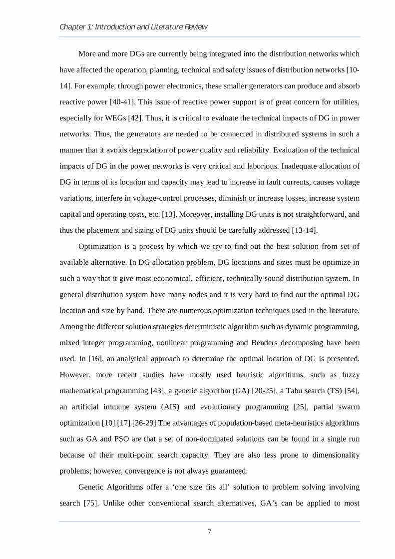
More and more DGs are currently being integrated into the distribution networks which
have affected the operation, planning, technical and safety issues of distribution networks [10-
14]. For example, through power electronics, these smaller generators can produce and absorb
reactive power [40-41]. This issue of reactive power support is of great concern for utilities,
especially for WEGs [42]. Thus, it is critical to evaluate the technical impacts of DG in power
networks. Thus, the generators are needed to be connected in distributed systems in such a
manner that it avoids degradation of power quality and reliability. Evaluation of the technical
impacts of DG in the power networks is very critical and laborious. Inadequate allocation of
DG in terms of its location and capacity may lead to increase in fault currents, causes voltage
variations, interfere in voltage-control processes, diminish or increase losses, increase system
capital and operating costs, etc. [13]. Moreover, installing DG units is not straightforward, and
thus the placement and sizing of DG units should be carefully addressed [13-14].
Optimization is a process by which we try to find out the best solution from set of
available alternative. In DG allocation problem, DG locations and sizes must be optimize in
such a way that it give most economical, efficient, technically sound distribution system. In
general distribution system have many nodes and it is very hard to find out the optimal DG
location and size by hand. There are numerous optimization techniques used in the literature.
Among the different solution strategies deterministic algorithm such as dynamic programming,
mixed integer programming, nonlinear programming and Benders decomposing have been
used. In [16], an analytical approach to determine the optimal location of DG is presented.
However, more recent studies have mostly used heuristic algorithms, such as fuzzy
mathematical programming [43], a genetic algorithm (GA) [20-25], a Tabu search (TS) [54],
an artificial immune system (AIS) and evolutionary programming [25], partial swarm
optimization [10] [17] [26-29].The advantages of population-based meta-heuristics algorithms
such as GA and PSO are that a set of non-dominated solutions can be found in a single run
because of their multi-point search capacity. They are also less prone to dimensionality
problems; however, convergence is not always guaranteed.
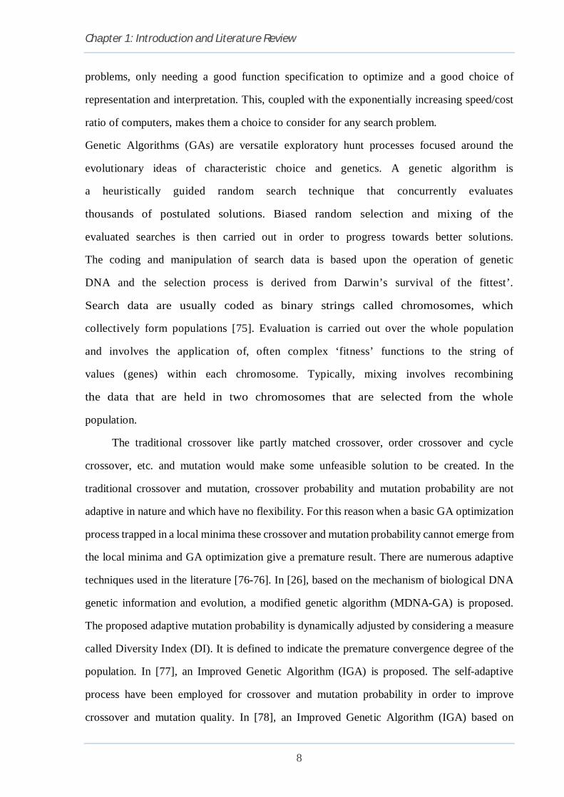
Genetic Algorithms offer a ‘one size fits all’ solution to problem solving involving
search [75]. Unlike other conventional search alternatives, GA’s can be applied to most
Chapter 1: Introduction and Literature Review
8
problems, only needing a good function specification to optimize and a good choice of
representation and interpretation. This, coupled with the exponentially increasing speed/cost
ratio of computers, makes them a choice to consider for any search problem.
Genetic Algorithms (GAs) are versatile exploratory hunt processes focused around the
evolutionary ideas of characteristic choice and genetics. A genetic algorithm is
a heuristically guided random search technique that concurrently evaluates
thousands of postulated solutions. Biased random selection and mixing of the
evaluated searches is then carried out in order to progress towards better solutions.
The coding and manipulation of search data is based upon the operation of genetic
DNA and the selection process is derived from Darwin’s survival of the fittest’.
Search data are usually coded as binary strings called chromosomes, which
collectively form populations [75]. Evaluation is carried out over the whole population
and involves the application of, often complex ‘fitness’ functions to the string of
values (genes) within each chromosome. Typically, mixing involves recombining
the data that are held in two chromosomes that are selected from the whole
population.
The traditional crossover like partly matched crossover, order crossover and cycle
crossover, etc. and mutation would make some unfeasible solution to be created. In the
traditional crossover and mutation, crossover probability and mutation probability are not
adaptive in nature and which have no flexibility. For this reason when a basic GA optimization
process trapped in a local minima these crossover and mutation probability cannot emerge from
the local minima and GA optimization give a premature result. There are numerous adaptive
techniques used in the literature [76-76]. In [26], based on the mechanism of biological DNA
genetic information and evolution, a modified genetic algorithm (MDNA-GA) is proposed.
The proposed adaptive mutation probability is dynamically adjusted by considering a measure
called Diversity Index (DI). It is defined to indicate the premature convergence degree of the
population. In [77], an Improved Genetic Algorithm (IGA) is proposed. The self-adaptive
process have been employed for crossover and mutation probability in order to improve
crossover and mutation quality. In [78], an Improved Genetic Algorithm (IGA) based on

Chapter 1: Introduction and Literature Review
9
hormone modulation mechanism is proposed in order to ensure to create a feasible solution, a
new method for crossover operation is adopted, named, partheno-genetic operation (PGO). .
The adaptive approaches proposed by Vedat Toğan and Ayşe T. Daloğlu [79] for crossover
and mutation operator of the GA. The performance of genetic algorithms (GA) is affected by
various factors such as coefficients and constants, genetic operators, parameters and some
strategies. Member grouping and initial population strategies are also examples of factors.
While the member grouping strategy is adopted to reduce the size of the problem, the initial
population strategy have been applied to reduce the number of search to reach the optimum
design in the solution space. In this study, two new self-adaptive member grouping strategies,
and a new strategy to set the initial population have been discussed. Chaogai Xue, Lili Dong
and Junjuan Liu [80] proposed an adaptive approaches for crossover and mutation operator of
the GA optimize enterprise information system (EIS) structure based on time property.
1.3.2 Uncertainty in Distribution Planning
In most of the planning models, the optimal distribution network is determined based on
a deterministic load demand which is usually obtained from a load forecast. The optimal DG
power generation of a distribution network is determined based on the DG generation (i.e.,
electric utilities and customers) and weather forecast in the form of wind or solar power
generation. However, such a forecast is always subject to some error. Since the operating
conditions (e.g. node voltage, branch current, illumination of sun, wind speed, etc.) of any
distribution network depend on the load, a network operating with loads that differ from the
nominal ones may be subject to violations of the acceptable operating conditions [1-2] [43].
Also the placement of the DG units mainly the Renewable energy sources placement, is
affected by several factors such as wind speed, solar irradiation, environmental factors,
geographical topography, political factors, etc. For example, wind generators or turbines cannot
be installed near residential areas, because of the interference in the form of public reactions
and legislations from environmental organisations. Another issue is application of the plug-in
electric vehicle (PEV) which is being paid more attention to [44-46]. However, there are
several factors or uncertainties that can possibly lead to probable risks in determining the

Chapter 1: Introduction and Literature Review
10
optimal siting and sizing of DGs in distribution system planning [47]. Some of the
uncertainties are possibilistic output power of a PEV due to its alteration of
charging/discharging schedule [48-50], wind power unit due to frequent variable wind speed,
from a solar generating source due to the possibilistic illumination intensity, volatile fuel
prices, uncertain electricity price and future uncertain load growth [51-52] [57]. The most
essential uncertainty to account for the time-varying characteristics of both generation and
demand of power are these increasing penetrations of variable renewable generators with wind
power [43] [47] [53], being the most noteworthy of them. In [53], the multiple objective
functions are aggregated to form a single objective function so as to optimize them. However,
in [54], the multiple objectives are simultaneously optimized to obtain a set of non-dominated
solutions, in which no solution is superior or inferior to others. The most of the approaches are
based on the constant power load model, except in [43], in which voltage dependent load model
is used.
1.4 ORGANIZATION OF THE REPORT
The work carried out in this Report has been summarized in six chapters.
The Chapter 2 highlights the brief introduction, summary of work carried out by various
researchers, and the outline of the thesis is also given in this chapter. The Chapter 3 explains
the Forward/Backward Load Flow Technique of distribution networks using BIBC and
BCBV matrix, Distributed generator planning, Genetic Algorithm. The Chapter 4 briefly
describes how to identify the candidate nodes for distributed generator placement,
objective function for overall loss minimization of distribute on networks, steps for
Distributed Generator (DG) Allocation using Genetic Algorithm, and results and discussion
pertaining to various test cases. The Chapter 5 details the uncertainty in distribution
planning. The conclusions and the scope of further work are detailed in Chapter 6.
11
CHAPTER-2
MODELLING AND ALLOCATION OF DG IN
DISTRIBUTION NETWORKS
2.1 INTRODUCTION
Loss Minimization in power networks has assumed greater significance, in light of the fact
that enormous amount of generated power is continuously squandered as losses. Studies have
demonstrated that 70% of the aggregate networks losses are happening in the distribution
networks, while transmission lines represent just 30% of the aggregate losses [1]. The
pressure of enhancing the overall proficiency of power delivery has forced the power
utilities to reduce the loss, particularly at the distribution level. The following approaches
are embraced for reduction of distribution networks losses [1-2].
Reinforcement of the feeders.
Reactive power compensation.
High voltage distribution networks.
Grading of conductor.
Feeder reconfiguration.
Distributed Generator placement.
Smart grid concept is expected to become a backbone in Europe future electricity network [10].
In achieving a Smart Grid concept, a large number of distributed generators (DG) are needed
inside distribution network which is prognosed to supply up to 40% of the distribution
network’s load demand. This substantial number of DG is obliged to take part in enhancing the
security, reliability and quality of electricity supply by providing active power and other
subordinate services such as regulating the voltage by providing their reactive supply to the
network. One of the characteristics of future electricity network under smart grid idea is to
have an efficient transmission and distribution network that will reduce line losses [3-9].
Minimizing losses inside power transport networks will being about easier utilization of fossil
fuel consequently reduced emanation of air pollutant and greenhouse gasses. Coordinating of
DG inside distribution network reduces power losses in light of the fact that some share of the

Chapter 2: Modelling and Allocation of DG in Distribution Network
12
required load current from upstream is generously reduce which result lower losses through
line resistance. Further reduction of losses can be attained by intelligently managing reactive
power from introduced DG [10].
2.2 DISTRIBUTION NETWORK POWER LOSSES
An active power loss in the line depends on magnitude of the current flows through the line
and resistance of the line. In ac distribution circuit, due to electric and magnetic field produce
by the flow of time varying current, inductance and capacitance might be noteworthy. At the
point when current flow through these two components, reactive power which transmit no
energy is produced. Reactive current flow in the line adds to extra power losses in addition to
active power losses mention previously. Integration of DG already reduced active power losses
because some portion of power from upstream is already reduced. Losses reduction can be
further reduced by controlling the voltage profiles in the network. In conventional practice,
capacitor banks are added in the distribution network to control the flow of this reactive power.
These capacitor banks can be switched in and out using voltage regulating relay to deliver
reactive power in steps but it lowered power quality delivered to the customer as it leads to step
changes in node-bar voltage.
푃 (푥) = ∑ 3 퐼 푅 ∀푖 = 푁 (1.1)
2.3 DISTRIBUTED GENERATION
2.3.1 Operational and Planning Issues with DGs
Distributed Generators (DG) are crisply characterized as "electric power sources joined
specifically to the distribution system or on the client side of the meter" [3]. This definition
for the most part obliges a variety of technologies and execution crosswise over diverse utility
structures, while evading the pitfalls of utilizing more stringent criteria focused around
standards, for example, power ratings and power delivery area. Distribution planning includes
the investigation of future power delivery needs and options, with an objective of creating a
precise course of action of increases to the networks required to attain agreeable levels of
service at a minimum overall cost [4]. Executing DGs in the distribution system has numerous

Chapter 2: Modelling and Allocation of DG in Distribution Network
13
profits, yet in the meantime it confronts numerous restrictions and limitations. DG units, being
adaptable, could be built to meet immediate needs and later be scaled upwards in capacity to
take care of future demand growth. Versatility permits DG units to reduce their capital and
operations costs and therefore substantial capital is not tied up in investments or in their
support infrastructure. Investment funds can likewise be accomplished since infrastructure
updates, (for example, feeder capacity extensions) might be deferred or altogether eliminated.
From a client perspective, funds may be gathered from the extra decision and flexibility that
DGs permit with respect to energy purchases [3-6]. On the other hand, then again, installing
DG in the distribution networks can also increase the complexity of networks planning. DG
must be satisfactorily introduced and facilitated with the existing protective devices and
schemes. Higher penetration levels of DG may cause conventional power flows to alter
(reverse direction), since with generation from DG units, power may be injected at any point
on the feeder. New planning systems must guarantee that feeders can suit changes in load
configuration. These limitations and problems must be settled before picking DG as a planning
alternative. Some of the associated issues in distribution networks with penetration of DG
units are as discussed next.
2.3.2 DG Operation
There are numerous components influencing DG operation, for example, DG technologies,
types, operational modes, and others. DGs installed in the distribution network can be owned,
operated and controlled by either an electric utility or a customer. In the event that DG is
utility-claimed, then its working cycle is well known as is controlled by the utility. The state
of the DG working cycle relies on upon the motivation behind its utilization in the distribution
system [3-9]. For example:
a) Limited operating time units for peak crest load shaving (Internal combustion engines, small
fuel cell units).
b) Limited operating time units to impart the load to diverse operating cycles (Micro-turbines
and fuel cells).
c) Base load power supply (Micro-turbines and large fuel cells).

Chapter 2: Modelling and Allocation of DG in Distribution Network
14
d) Renewable energy units influenced by ecological conditions, for example, wind speed and
sunlight respectively (Wind generators and solar cells)
On the other hand, customer-owned DG operating cycles are not known to the operators unless
there is a unit commitment agreement between the electric utility and the customer, which is
not very likely. Thus, small customer owned DG operating cycles are acknowledged to be
capricious processes from the perspective of the electric utility. The utility has no control on
their operation. This uncertainty changes the planning and operation problem from a
deterministic problem to a non-deterministic one.
2.3.3 DG Siting
There are no agreeable limitations on location of DG units in the distribution system, as there
are no geological limitations as on account of substations. Subsequently, the main limitations
emerge from electrical necessities. In the event that the DG is client possessed then the utility
has no control on its location in light of the fact that it is put at the client's site. In the event
that the DG is utility-possessed then the choice of its location is focused around a few electrical
factors, for example:
• Providing the required extra load demand
• Reducing networks losses
• Enhancing networks voltage profile and expanding substations capacities
Likewise, DG units must be put on feeders that don't affect the existing protective device co-
ordinations and ratings.
2.3.4 DG Sizing
There are no clear guidelines on selecting the size and number of DG units to be introduced
in the network. However, a few aspects can be guiding the choice of DG unit size selection:
a) To enhance the networks voltage profile and reduce power losses, it is sufficient to utilize
DG units of aggregate capacity in the reach of 10-20% of the aggregate feeder demand [3].
While more DG capacity could be utilized to reduce the substation loading [3-9].

Chapter 2: Modelling and Allocation of DG in Distribution Network
15
b) For reliability purposes if there should arise an occurrence of islanding, the DG size must
be greater than double the required island load. The DG unit size can affect networks
protection coordination schemes and devices as it affects the value of the short circuit
current during fault.
Hence, as the DG size increases, the protection devices, fuses, re-closers and relays settings
have to be readjusted and/or overhauled [1-2].

Chapter 2: Modelling and Allocation of DG in Distribution Network
16
2.4 SUMMARY
In this chapter discusses the relevant issues and aims at providing a general definition for
distributed power generation in competitive electricity markets. In general, DG can be defined
as electric power generation within distribution networks or on the customer side of the
network. In addition, the terms distributed resources, distributed capacity and distributed utility
are discussed.

17
CHAPTER-3
INCORPORATION OF DG MODEL IN DISTRIBUTION
NETWORK LOAD FLOWS
3.1 INTRODUCTION
The load flow of a power system gives the unfaltering state result through which
different parameters of investment like currents, voltages, losses and so on can be
figured. The load flow will be imperative for the investigation of distribution
networks, to research the issues identified with planning, outline and the operation
and control. A few provisions like ideal distributed generation placement in distribution
networks and distribution automation networks, obliges rehashed load flow result.
Numerous systems such Gauss-Seidel, Newton-Raphson are generally appeared for
convey the load flow of transmission networks [1]. The utilization of these systems for
distribution networks may not be worthwhile in light of the fact that they will be
generally focused around the general meshed topology of a normal transmission
networks although most distribution networks structure are likely in tree, radial or
weakly meshed in nature. R/X ratio of distribution networks is high respect to
transmission system, which cause the distribution networks to be badly molded for
ordinary load flow techniques[1-2]. Some other inborn aspects of electric distribution
networks are (i) radial or weakly meshed structure, (ii) unbalanced operation and unbalanced
distributed loads, (iii) large number of nodes and branches, (iv) has wide range of resistance
and reactance values and (v) distribution networks has multiphase operation.
The effectiveness of the optimization problem of distribution networks relies on upon the
load flow algorithm on the grounds that load flow result need to run for ordinarily. Thusly,
the load flow result of distribution networks ought to have ronodet and time proficient
qualities. A technique which can discover the load flow result of radial distribution networks
specifically by utilizing topological normal for distribution system [69-70] [72-74] is
utilized. In this strategy, the plan of tedious Jacobian matrix or admittance matrix, which are
needed in customary techniques, is stayed away from. This system is illustrated in a nutshell.

Chapter 3: Incorporation of DG Model in Distribution System Load Flows
18
3.2 LOAD FLOW OF RADIAL DISTRIBUTION NETWORKS A feeder brings power from substation to load points/nodes in radial distribution
networks (RDN). Single or multiple radial feeders are used in this planning approach.
Basically, the RDN total power losses can be minimized by minimizing the branch power flow
or transported electrical power from transmission networks (i.e. some percentage of load are
locally meeting by local DG). To determine the total power loss of the network or each feeder
branch and the maximum voltage deviation are determined by performing load flow. The
Forward/Backward Sweep Load Flow technique is used in this case. The impedance of a feeder
branch is computed by the specified resistance and reactance of the conductors used in the
branch construction. The Forward/Backward Sweep Load Flow method consist two steps (i)
backward sweep and (ii) forward sweep.
Backward sweep: In this step, the load current of each node of a distribution network having
N number of nodes is determined as:
퐼 ̅ (푚) = ( ) ( )∗( )
[푚 = 1,2,3 … … …푁] (3.1)
where, 푃 (푚) and 푄 (푚) represent the active and reactive power demand at node m and the
overbar notation (푥̅) indicates the phasor quantities, such as 퐼 ̅ ,푉∗.Then, the current in each
branch of the network is computed as:
퐼(̅푚푛) = 퐼 ̅ (푛) + ∑ 퐼 ̅ (푚)∈ (3.2)
where, the setΓ consists of all nodes which are located beyond the node n [32].
Forward sweep: This step is used after the backward sweep so as to determine the voltage at
each node of a distribution network as follows:
푉(푛) = 푉(푚)− 퐼(̅푚푛)푍(푚푛) (3.3)
where, nodes n and m represent the receiving and sending end nodes, respectively for the branch
mn and 푍(푚푛) is the impedance of the branch.
In this work the estimation methodology utilized within the forward/backward load
flow is based on (i) equivalent current injections (ECI), (ii) the node-injection to branch-
current matrix (BIBC) and (ii) the branch-current to node-voltage matrix (BCBV). In this
area, the advancement methodology will be depicted in subtle element. Load flow for

Chapter 3: Incorporation of DG Model in Distribution System Load Flows
19
distribution networks under balanced operating condition with constant power load model
can be under remained through the accompanying focuses:
3.2.1 Equivalent Current Injection
The technique is based on the equivalent current injection of a node in distribution
networks, the equivalent-current-injection model is more practical [69-70] [73]. For any
node of distribution networks, the complex load 푆 is expressed by
푆 = 푃 + 푗푄 푖 = 1, … … …푁 (3.4)
Now, the equivalent current injection is expressed as
퐼 = 퐼 (푉 ) + 푗퐼 (푉 ) = ∗푖 = 1, … … …푁 (3.5)
For the load flow solution equivalent current injection (ECI) at the k-th iteration at i-th node
is computed as
퐼 = 퐼 (푉 ) + 푗퐼 (푉 ) = ∗ (3.6)
3.2.2 Formation of BIBC Matrix
The power injections at every node might be transformed into the equivalent current
injections using the eq. (3.6) and applying Kirchhoff’s Current Law (KCL) at each and
every node a set of comparisons could be composed. Now each and every branch currents
of the network can be shaped as a function of the equivalent current injections (ECI) [69-
70] [73]. As shown in Figure 3.1, the branch currents IB5, IB4, IB3, IB2 and IB1 can be
expressed as:
퐼퐵 = 퐼 (3.7)
퐼퐵 = 퐼 (3.8)
퐼퐵 = 퐼 + 퐼 (3.9)
퐼퐵 = 퐼 + 퐼 + 퐼 + 퐼 (3.10)
퐼퐵 = 퐼 + 퐼 + 퐼 + 퐼 + 퐼 (3.11)
Chapter 3: Incorporation of DG Model in Distribution System Load Flows
20
From the above equations () the BIBC matrix can be written as:
⎣⎢⎢⎢⎡퐼퐵퐼퐵퐼퐵퐼퐵퐼퐵 ⎦
⎥⎥⎥⎤
=
⎣⎢⎢⎢⎡1111101111001100001000001⎦
⎥⎥⎥⎤
⎣⎢⎢⎢⎡퐼퐼퐼퐼퐼 ⎦⎥⎥⎥⎤
(3.12)
The general form as of eq. (3.12) can be expressed as:
[퐼퐵] = [퐵퐼퐵퐶][퐼] (3.13)
The detailing of BIBC matrix for distribution networks demonstrated in Figure 3.1 is
given in eq. (3.13). For general network, the BIBC matrix might be shaped through the
accompanying steps and the example is done by the help of Figure 3.1:
Step 1: Make an initial null BIBC matrix with a dimension of(푚 × (푛 − 1)). Where m and
n are the number of branches and nodes available in the network.
Step 2: initially set i=1 and read the IBi (i=1, 2, 3…m) branch data (i.e. sending end and
receiving end node) from line-data matrix. If a line section IBi is located between
Node ‘x’ and Node ‘y’. Check, that the IBi branch section of the network is belongs
to the first node of the network or not. If it is, then make the (y-1, y-1)-th bit of BIBC
matrix by ‘+1’. Increment ‘i’ by one or go to the step#3.
Step 3: If the in step#2 the IBi branch section is not belongs to the first node of the
network. Then copy the column segment of the ‘(x-1)-th’ node of BIBC matrix
to the column segment of ‘(y-1)-th’ node and fill (y-1, y-1)-th bit of the BIBC
Figure 3.1. Simple distribution system

Chapter 3: Incorporation of DG Model in Distribution System Load Flows
21
matrix by ‘+1’. Increment ‘i’ by one and go to the step#2. This is explained in fig
3.2
Step 4: Repeat step#2 and step#3 until all the branches of the network included in to the
BIBC matrix.
3.2.3 Formation of BCBV matrix
The Branch-Current to Node voltage (BCBV) matrix summarizes the relation
between branch current and node voltages. The relations between the branch currents
and node voltages can be obtained easily by applying Kirchhoff’s Voltage Law (KVL).
As shown in Figure 3.1, the voltages of Node 2, 3, and 4 are expressed as:
푉 = 푉 − 퐼퐵 푍 (3.14)
푉 = 푉 − 퐼퐵 푍 (3.15)
푉 = 푉 − 퐼퐵 푍 (3.16)
Step#1
0 0 0 0 0
i=1
1 0 0 0 0
i=2
1 1 0 0 0
→
1 1 0 0 0 0 0 0 0 0 0 0 0 0 0 0 0 0 0 0 0 1 0 0 0 0 0 0 0 0 0 0 0 0 0 0 0 0 0 0 0 0 0 0 0 0 0 0 0 0 0 0 0 0 0 0 0 0 0 0 0 0 0 0 0 0 0 0 0 0 0 0 0 0 0 0 0 0 0 0 0 0 0 0 0 In step#2 Copy 1st column In step#3
i=3
1 1 1 0 0
→
1 1 1 0 0
i=4
1 1 1 1 0
→
1 1 1 1 0 0 1 1 0 0 0 1 1 0 0 0 1 1 1 0 0 1 1 1 0 0 0 0 0 0 0 0 1 0 0 0 0 1 1 0 0 0 1 1 0 0 0 0 0 0 0 0 0 0 0 0 0 0 0 0 0 0 0 1 0 0 0 0 0 0 0 0 0 0 0 0 0 0 0 0 0 0 0 0 0
Copy 2nd column In step#3 Copy 2nd column In step#3
i=5
1 1 1 0 0
→
1 1 1 1 1
Branch no Sending node Receiving node
0 1 1 0 0 0 1 1 1 1 0 0 0 0 0 0 0 1 1 0 1 1 2 0 0 0 0 0 0 0 0 1 0 2 2 3 0 0 0 0 0 0 0 0 0 1 3 3 4
Copy 2nd column In step#3 4 4 5 5 3 6
Copied column Updated column
Figure 3.2. The formation of BIBC matrix, the example is done by the help of Figure 3.1.

Chapter 3: Incorporation of DG Model in Distribution System Load Flows
22
Substituting equations (3.14) and (3.15) into eqn. (3.16), the voltage of Node 4 can be
rewritten as:
푂푟,푉 = 푉 − 퐼퐵 푍 − 퐼퐵 푍 − 퐼퐵 푍 (3.17)
From equation it can be seen that the node voltage of the network can be expressed as a
function of the branch currents, line parameters and main substation voltage. Similar
approach can be employed for other nodes, and the Branch-Current to Node-Voltage (BCBV)
matrix can be derived as:
⎣⎢⎢⎢⎡푉푉푉푉푉 ⎦⎥⎥⎥⎤
−
⎣⎢⎢⎢⎡푉푉푉푉푉 ⎦⎥⎥⎥⎤
=
⎣⎢⎢⎢⎡푍 0000푍 푍 000푍 푍 푍 00푍 푍 푍 푍 0푍 푍 00푍 ⎦
⎥⎥⎥⎤
⎣⎢⎢⎢⎡퐼퐵퐼퐵퐼퐵퐼퐵퐼퐵 ⎦
⎥⎥⎥⎤
(3.18)
The general form of eq. (3.18) can be expressed as:
푂푟, [∆푉] = [퐵퐶퐵푉][퐼퐵] (3.19)
The formulation of BCBV matrix for distribution networks shown in Figure 3.1 is given eq.
(3.18) and eq. (3.19). For universal network, the BCBV matrix can be formed through
the subsequent steps:
Step 1: Make an initial null BVBC matrix with a dimension of((푛 − 1) × 푚). Where m and
n are the number of branches and nodes available in the network.
Step 2: initially set i=1 and read the IBi (i=1, 2, 3…m) branch data (i.e. sending end and
receiving end node) from line-data matrix. If a line section IBi is located between
Node ‘x’ and Node ‘y’. Check, that the IBi branch section of the network is belongs
to the first node of the network or not. If it is, then make the (y-1, y-1)-th bit of BVBC
matrix by the corresponding branch impedance (Zxy). Increment ‘i’ by one or go to the
step#3.
Step 3: If the in step#2 the IBi branch section is not belongs to the first node of the
network. Then copy the row segment of the ‘(x-1)-th’ node of BVBC matrix to
the row segment of ‘(y-1)-th’ node and fill (y-1, y-1)-th bit of the BVBC matrix
by the corresponding branch impedance (Zxy). Increment ‘i’ by one and go to the
step#2. This is explained in Figure 3.2.
Chapter 3: Incorporation of DG Model in Distribution System Load Flows
23
Step 4: Repeat step#2 and step#3 until all the branches of the network included in the
BVBC matrix.
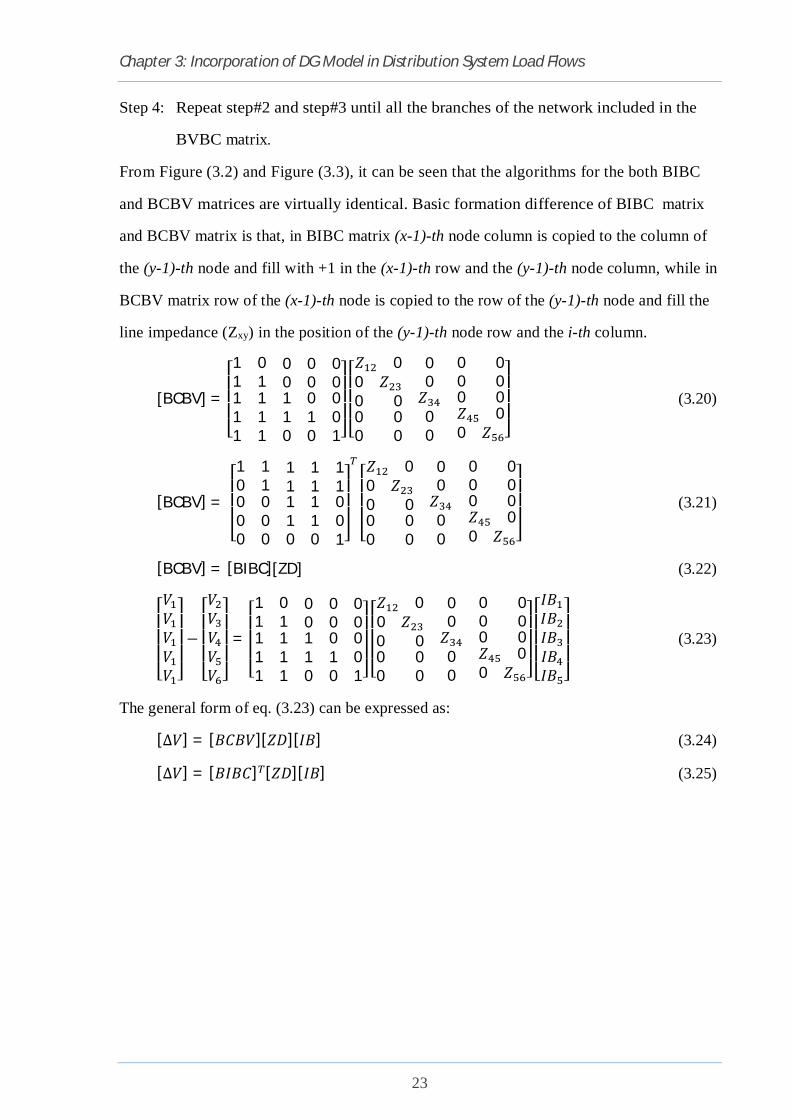
From Figure (3.2) and Figure (3.3), it can be seen that the algorithms for the both BIBC
and BCBV matrices are virtually identical. Basic formation difference of BIBC matrix
and BCBV matrix is that, in BIBC matrix (x-1)-th node column is copied to the column of
the (y-1)-th node and fill with +1 in the (x-1)-th row and the (y-1)-th node column, while in
BCBV matrix row of the (x-1)-th node is copied to the row of the (y-1)-th node and fill the
line impedance (Zxy) in the position of the (y-1)-th node row and the i-th column.
[BCBV] =
⎣⎢⎢⎢⎡1 0 0 0 01 1 0 0 0111
111
110
010
001⎦⎥⎥⎥⎤
⎣⎢⎢⎢⎡푍 00 푍0 00 00 0
00푍
00
0 00 00 0푍 00 푍 ⎦
⎥⎥⎥⎤ (3.20)
[BCBV] =
⎣⎢⎢⎢⎡1 1 1 1 10 1 1 1 1000
000
110
110
001⎦⎥⎥⎥⎤
⎣⎢⎢⎢⎡푍 00 푍0 00 00 0
00푍
00
0 00 00 0푍 00 푍 ⎦
⎥⎥⎥⎤ (3.21)
[BCBV] = [BIBC][ZD] (3.22)
⎣⎢⎢⎢⎡푉푉푉푉푉 ⎦⎥⎥⎥⎤
−
⎣⎢⎢⎢⎡푉푉푉푉푉 ⎦⎥⎥⎥⎤
=
⎣⎢⎢⎢⎡1 0 0 0 01 1 0 0 0111
111
110
010
001⎦⎥⎥⎥⎤
⎣⎢⎢⎢⎡푍 00 푍0 00 00 0
00푍
00
0 00 00 0푍 00 푍 ⎦
⎥⎥⎥⎤
⎣⎢⎢⎢⎡퐼퐵퐼퐵퐼퐵퐼퐵퐼퐵 ⎦
⎥⎥⎥⎤
(3.23)
The general form of eq. (3.23) can be expressed as:
[∆푉] = [퐵퐶퐵푉][푍퐷][퐼퐵] (3.24)
[∆푉] = [퐵퐼퐵퐶] [푍퐷][퐼퐵] (3.25)

Chapter 3: Incorporation of DG Model in Distribution System Load Flows
24
3.2.4 Solution Methodology
The development of BIBC and BCBV matrices is clarified in section 3.2.2 and 3.2.3. These
matrices investigate the topological structure of distribution networks. Basically the BIBC
matrix is making an easy relation between the node current injections and branch currents.
These relation give a simple solution for branch currents variation, which is occurs due to the
variation at the current injection nodes, these can be obtained directly by using BIBC matrix.
The BCBV matrix build an effective relations between the branch currents and node voltages.
The concern variation of the node voltages is produced by the variant of the branch currents.
These could be discovered specifically by utilizing the BCBV matrix. Joining eqs. (3.13) and
(3.19), the relations between the node current injections and node voltages could be
communicated as:
[∆푉] = [퐵퐶퐵푉]. [퐵퐼퐵퐶]. [퐼] (3.26)
Step#1
0 0 0 0 0
i=1
Z12 0 0 0 0
i=2
Z12 0 0 0 0
→
Z12 0 0 0 0 0 0 0 0 0 0 0 0 0 0 Z12 0 0 0 0 Z12 Z23 0 0 0 0 0 0 0 0 0 0 0 0 0 0 0 0 0 0 0 0 0 0 0 0 0 0 0 0 0 0 0 0 0 0 0 0 0 0 0 0 0 0 0 0 0 0 0 0 0 0 0 0 0 0 0 0 0 0 0 0 0 0 0
In step#2 Copy 1st row In step#3
i=3
Z12 0 0 0 0
→
Z12 0 0 0 0
i=4
Z12 0 0 0 0
→
Z12 0 0 0 0 Z12 Z23 0 0 0 Z12 Z23 0 0 0 Z12 Z23 0 0 0 Z12 Z23 0 0 0 Z12 Z23 0 0 0 Z12 Z23 Z34 0 0 Z12 Z23 Z34 0 0 Z12 Z23 Z34 0 0 0 0 0 0 0 0 0 0 0 0 Z12 Z23 Z34 0 0 Z12 Z23 Z34 Z45 0 0 0 0 0 0 0 0 0 0 0 0 0 0 0 0 0 0 0 0 0
Copy 2nd crow In step#3 Copy 2nd row In step#3
i=5
Z12 0 0 0 0
→
Z12 0 0 0 0
Branch no Sending node
Receiving node Z12 Z23 0 0 0 Z12 Z23 0 0 0
Z12 Z23 Z34 0 0 Z12 Z23 Z34 0 0 1 1 2 Z12 Z23 Z34 Z45 0 Z12 Z23 Z34 Z45 0 2 2 3 Z12 Z23 0 0 0 Z12 Z23 0 0 Z56 3 3 4
Copy 2nd row In step#3 4 4 5 5 3 6
Copied row Updated row
Figure 3.3. The formation of BVBC matrix, the example is done by the help of Figure 3.1.

Chapter 3: Incorporation of DG Model in Distribution System Load Flows
25
푁표푤 [퐵퐶퐵푉] = [퐵퐼퐵퐶] . [푍퐷] (3.27)
∴ [∆푉] = [퐵퐼퐵퐶] . [푍퐷]. [퐵퐼퐵퐶]. [퐼] (3.28)
∴ [퐷퐿퐹] = [퐵퐶퐵푉][퐵퐼퐵퐶] (3.29)
∴ [퐷퐿퐹] = [퐵퐼퐵퐶] . [푍퐷]. [퐵퐼퐵퐶] (3.30)
푇ℎ푒푟푒푓표푟 [∆푉] = [퐷퐿퐹]. [퐼] (3.31)
The iterative solution for the distribution system load flow can be obtained by solving eqs.
(3.32) and (3.33) which are specified below:
퐼 = 퐼 (푉 ) + 푗퐼 (푉 ) = 푃 + 푗푄
푉
∗
(3.32)
[∆푉 ] = [퐷퐿퐹]. [퐼 ] (3.33)
[푉 ] = [푉 ] + [∆푉 ] (3.33)
The new definition as illustrated uses just the DLF matrix to take care of load flow
problem. Subsequently this strategy is extremely time efficient, which is suitable for on-
line operation and optimization problem of distribution networks.

Chapter 3: Incorporation of DG Model in Distribution System Load Flows
26
3.3 ALGORITHM FOR DISTRIBUTION NETWORKS LOAD FLOW
The algorithm steps for load flow solution of distribution networks is given below:
Step 1: Read the distribution networks line data and bus data.
Step 2: Calculate the each node current or node current injection matrix. The relationship
can be expressed as –
[퐼] =푆푉
∗
=푃 − 푗푄푉∗
Step 3: Calculate the BIBC matrix by using steps given in section 3.2.2.
Step 4: Evaluate the branch current by using BIBC matrix and current injection matrix
(ECI). The relationship can be expressed as -
[퐼퐵] = [퐵퐼퐵퐶][퐼]
Step 5: Form the BCBV matrix by using steps given in section 3.2.3. The relationship
therefore can be expressed as -
[∆푉] = [퐵퐶퐵푉][퐼퐵]
Step 6: Calculate the DLF matrix by using the eq. (3.30). The relationship will be -
[퐷퐿퐹] = [퐵퐶퐵푉][퐵퐼퐵퐶]
[∆푉] = [퐷퐿퐹][퐼]
Step 7: Set Iteration k = 0.
Step 8: Iteration k = k + 1.
Step 9: Update voltages by using eqs. (3.32), (3.33), (3.34), as –
퐼 = 퐼 (푉 ) + 푗퐼 (푉 ) = 푃 + 푗푄
푉
∗
[∆푉 ] = [퐷퐿퐹]. [퐼 ]
[푉 ] = [푉 ] + [∆푉 ]
Step 10: If max (|푉(푘 + 1)|− |푉(푘)|) > 푡표푙푒푟푎푛푐푒 go to step 6.
Step 11: Calculate branch currents, and losses from final node voltages.
Step 12: Display the node voltage magnitudes and angle, branch currents and losses.
Step 13: Stop
The above algorithm steps are shown in Flowchart given as Figure 3.4.

Chapter 3: Incorporation of DG Model in Distribution System Load Flows
27
Figure 3.4. Flowchart for load flow solution for radial distribution networks.
START
Calculate the equivalent current injection matrix;
Calculate BIBC matrix by the backward sweep method;
Calculate BCBV matrix by forward sweep method;
Calculate DLF Matrix and Set iteration k = 0;
Iteration k = k+1
|V (k+1)|-|V (k)|
>tolerance?
STOP
NO
Update Voltages
YES
Calculate line flow & losses using final node voltages;
Read System Input Data;
Chapter 3: Incorporation of DG Model in Distribution System Load Flows
28
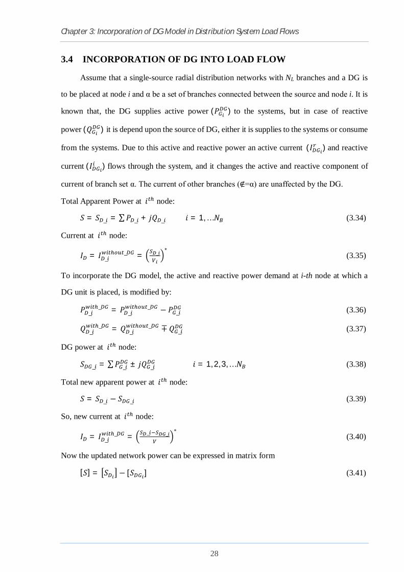
3.4 INCORPORATION OF DG INTO LOAD FLOW
Assume that a single-source radial distribution networks with NL branches and a DG is
to be placed at node i and α be a set of branches connected between the source and node i. It is
known that, the DG supplies active power (푃 ) to the systems, but in case of reactive
power(푄 ) it is depend upon the source of DG, either it is supplies to the systems or consume
from the systems. Due to this active and reactive power an active current(퐼 )and reactive
current(퐼 )flows through the system, and it changes the active and reactive component of
current of branch set α. The current of other branches (∉=α) are unaffected by the DG.
Total Apparent Power at 푖 node:
푆 = 푆 _ = ∑푃 _ + 푗푄 _ 푖 = 1, …푁 (3.34)
Current at 푖 node:
퐼 = 퐼 __ = _
∗ (3.35)
To incorporate the DG model, the active and reactive power demand at i-th node at which a
DG unit is placed, is modified by:
푃 __ = 푃 _
_ − 푃 _ (3.36)
푄 __ = 푄 _
_ ∓푄 _ (3.37)
DG power at 푖 node:
푆 _ = ∑푃 _ ± 푗푄 _ 푖 = 1, 2, 3, …푁 (3.38)
Total new apparent power at 푖 node:
푆 = 푆 _ − 푆 _ (3.39)
So, new current at 푖 node:
퐼 = 퐼 __ = _ _
∗ (3.40)
Now the updated network power can be expressed in matrix form
[푆] = 푆 − [푆 ] (3.41)

Chapter 3: Incorporation of DG Model in Distribution System Load Flows
29
3.5 INCORPORATION OF ON-LINE LOAD TAP CHANGER (OLTC) INTO LOAD FLOW
OLTC is generally placed in the line of a distribution system. Let, a OLTC is placed in a
line and it have the off-nominal tap ratio of (1:a) with a series admittance of YtI as shown in
Fig.4. We know that there is a direct relations between [ZD] and [B]. If an OLTC is placed in
a line then the transformer can be represented by a series admittance (YtI) in per unit as per the
휋model representation of OLTC [69-70] [73]. The off-nominal tap ratio of OLTC, per unit
admittance of both side of the transformer is different, and it force to change the admittance to
include the effect of off-nominal ratio. It’s have a direct effect of the line current, for
modification in the line admittance, line current relation need to be modified.
The modified impedance matrix including the per unit series impedance Z2nI of OLTC with the
line impedance
[푍퐷] =푍 + 0 0 0
0 (푍 + 0) 00 0 (푍 + 푍 )/푎
(3.42)
1
2naYt
Z
Yta
1aVI 2nn0
Yta
1aVI 220
Figure 3.5. Network with off-nominal tap changing transformer.

Chapter 3: Incorporation of DG Model in Distribution System Load Flows
30
In Figure 3.5. 퐼 푎푛푑퐼 are non-tap to tap side currents are diverging from nodes i and
n respectively. The modified equivalent current injection matrix including the off-nominal ratio
is
[퐵] = [퐵퐼퐵퐶]퐼 − 퐼퐼 − 0퐼 − 퐼
= [퐵퐼퐵퐶]
⎣⎢⎢⎡퐼 − 푌 푉
퐼퐼 − 푉 푉 ⎦
⎥⎥⎤ (3.43)
3.6 INCORPORATION OF CAPACITOR BANK INTO LOAD FLOW
Assume that a single-source radial distribution networks with NB branches and a capacitor
bank is to be placed at node i. The capacitor bank produces reactive power (푄 _ )due to this a
reactive current(퐼 )flow through the radial network branches which changes the reactive
component of current of branch. To incorporate the capacitor bank model, the reactive power
demand at i-th node at which a capacitor bank unit is placed, is modified by:
푄 __ = 푄 _
_ −푄 _ (3.44)
[푆] = 푆 − [푆 ] (3.45)
3.7 ALGORITHM FOR DISTRIBUTION NETWORKS LOAD FLOW WITH DG
The algorithm steps for load flow solution of distribution networks is given below:
Step 1: Read the distribution networks line data and bus data.
Step 2: Calculate DG power and capacitor bank power for each nodes and update the
system bus data.
Step 3: Calculate the total power demand with DG or capacitor bank or with both by the
help of eq. (3.41) (3.45). The relationship can be expressed as –
[푆] = 푆 − 푆 − [푆 ]
Step 4: Calculate the each node current or node current injection matrix. The relationship
can be expressed as –
[퐼] =푆푉
∗
=푃 − 푗푄푉∗

Chapter 3: Incorporation of DG Model in Distribution System Load Flows
31
Step 5: Calculate the modified impedance matrix and modified current injection matrix
for tap changer by the help of eq. (3.42) (3.43).
Step 6: Calculate the BIBC matrix by using steps given in section 3.2.2.
Step 7: Evaluate the branch current by using BIBC matrix and current injection matrix
(ECI). The relationship can be expressed as -
[퐼퐵] = [퐵퐼퐵퐶][퐼]
Step 8: Form the BCBV matrix by using steps given in section 3.2.3. The relationship
therefore can be expressed as -
[∆푉] = [퐵퐶퐵푉][퐼퐵]
Step 9: Calculate the DLF matrix by using the eq. (3.30). The relationship will be -
[퐷퐿퐹] = [퐵퐶퐵푉][퐵퐼퐵퐶]
[∆푉] = [퐷퐿퐹][퐼]
Step 10: Set Iteration k = 0.
Step 11: Iteration k = k + 1.
Step 12: Update voltages by using eqs. (3.32), (3.33), (3.34), as –
퐼 = 퐼 (푉 ) + 푗퐼 (푉 ) = 푃 + 푗푄
푉
∗
[∆푉 ] = [퐷퐿퐹]. [퐼 ]
[푉 ] = [푉 ] + [∆푉 ]
Step 13: If max (|푉(푘 + 1)|− |푉(푘)|) > 푡표푙푒푟푎푛푐푒 go to step 6.
Step 14: Calculate branch currents, and losses from final node voltages.
Step 15: Display the node voltage magnitudes and angle, branch currents and losses.
Step 16: Stop
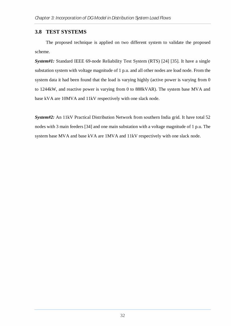
Chapter 3: Incorporation of DG Model in Distribution System Load Flows
32
3.8 TEST SYSTEMS
The proposed technique is applied on two different system to validate the proposed
scheme.
System#1: Standard IEEE 69-node Reliability Test System (RTS) [24] [35]. It have a single
substation system with voltage magnitude of 1 p.u. and all other nodes are load node. From the
system data it had been found that the load is varying highly (active power is varying from 0
to 1244kW, and reactive power is varying from 0 to 888kVAR). The system base MVA and
base kVA are 10MVA and 11kV respectively with one slack node.
System#2: An 11kV Practical Distribution Network from southern India grid. It have total 52
nodes with 3 main feeders [34] and one main substation with a voltage magnitude of 1 p.u. The
system base MVA and base kVA are 1MVA and 11kV respectively with one slack node.
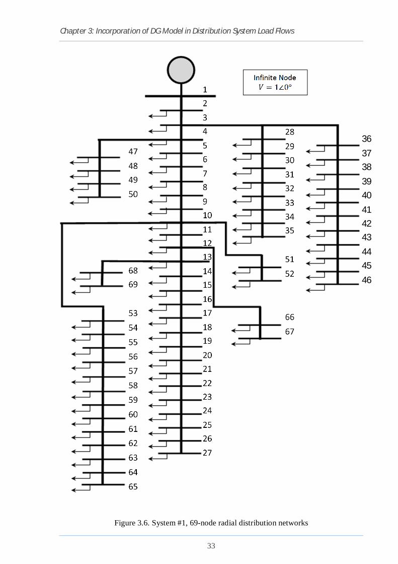
Chapter 3: Incorporation of DG Model in Distribution System Load Flows
33
Figure 3.6. System #1, 69-node radial distribution networks
Infinite Node 푉 = 1∠0° 1
2 3 4 5 6 7 8 9 10 11 12 13 14 15 16 17 18 19 20 21 22 23 24 25 26 27
36 37 38 39 40 41 42 43 44 45 46
28 29 30 31 32 33 34 35 51 52 66 67
47 48 49 50 68 69 53 54 55 56 57 58 59 60 61 62 63 64 65

Chapter 3: Incorporation of DG Model in Distribution System Load Flows
34
THUKARAM et al.: ARTIFICIAL NEURAL NETWORK AND SUPPORT VECTOR MACHINE APPROACH
Figure 3.7. System #2, 52-node radial distribution networks
Bus 46
Bus 48
Bus 45
Bus 44
Bus 43
Bus 42
Bus 50
Bus 47
Bus 52
Bus 49
Bus 51
Bus 36
Bus 38
Bus 34
Bus 40 Bus 41
Bus 35
Bus 39
Bus 37
Bus 33
Bus 32 Bus 3
Bus 2
Bus 5
Bus 4 Bus 1
Bus 20
Bus 27
Bus 28
Bus 29
Bus 31
Bus 30
Bus 21
Bus 22
Bus 23
Bus 24
Bus 11
Bus 15
Bus 18 Bus 17 Bus 25
Bus 26 Bus 12
Bus 13 Bus 14
Bus 19
Bus 6
Bus 7
Bus 16
Bus 8
Bus 9
Bus 10
Feeder 3
Feeder 2
Feeder 1

Chapter 3: Incorporation of DG Model in Distribution System Load Flows
35
3.9 LOAD FLOW SOLUTION FOR BASE CASE
System #1: The total load of the networks is 4.660MW (3802.19 kW active power and
2694.6kVAR reactive power) and the slack node is delivering 4.902MW power. The
distribution loss in the networks is 0.247 MW. The power loss due to active component of
current is 224.995 kW and power loss due to reactive component of the current is 102.198
kVAR. All node voltages are within 0.90919 - 1p.u. Also the minimum voltage is 0.90919 p.u.
is bearing the 65th number node of the system and the maximum branch current 0.49031p.u is
bearing by the branch 1.The MATLAB® simulation result are shown in Figure 3.8 and Figure
3.9. The load flow study is carried out with an accuracy level of 10^-9, and maximum iteration
of 300. The convergence of load flow with the accuracy level occur at 9 iteration. The Table
3.1 contains the node voltage magnitudes, branch current magnitudes, and the angle in radian
of the converged load flow solutions. The results shows that, at the peak load condition system
performance is not so poor. The system have a poor voltage profile at node 57 to node 65 due
to the system hugely loaded at 61 node. While some of the node have no load.
System#2: The total load of the networks is 4.648 MW (4184 kW active power and 2025
kVAR reactive power) and the slack node is delivering 5.613 MW power. The distribution loss
in the networks is 0.9658 MW. The power loss due to active component of current is 887.181
kW and power loss due to reactive component of the current is 381.694 kVAR. All node
voltages are within 0.68442 - 1p.u. also the minimum voltage of 0.68442 p.u. is occurs at the
50th node and the maximum branch current of 2.4382 p.u flows through the 31th branch. The
MATLAB® simulation result are shown in Figure 3.10 and Figure 3.11. In this case also the
load flow study is carried out with an accuracy level of 10^-9, and maximum iteration of 300.
The convergence of load flow with the accuracy level also occur at 9 iteration. The Table 3.2
contains the node voltage magnitudes, branch current magnitudes, and the angle in radian of
the converged load flow solutions. The results shows that, at the peak load condition system
performance is very poor. The system have a poor voltage profile at most of the nodes, basically
at 5 to 19 and 32 to 52 nodes.

Chapter 3: Incorporation of DG Model in Distribution System Load Flows
36
Figure 3.8. Base case node voltage magnitudes of system#1
0 10 20 30 40 50 60 700.9
0.91
0.92
0.93
0.94
0.95
0.96
0.97
0.98
0.99
11.005
Node Number
Vol
tage
Mag
nitu
de (p
.u.)
Figure 3.9. Base case branch current magnitudes of system#1
0 10 20 30 40 50 60 700
0.05
0.1
0.15
0.2
0.25
0.3
0.35
0.4
0.45
0.5
Node Number
Curr
ent M
agni
tude
(p.u
.)
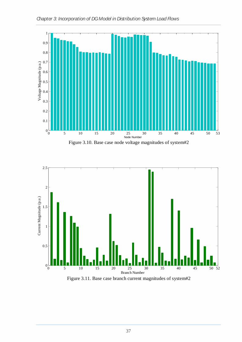
Chapter 3: Incorporation of DG Model in Distribution System Load Flows
37
Figure 3.10. Base case node voltage magnitudes of system#2
0 5 10 15 20 25 30 35 40 45 50 530
0.1
0.2
0.3
0.4
0.5
0.6
0.7
0.8
0.9
1
Node Number
Vol
tage
Mag
nitu
de (p
.u.)
Figure 3.11. Base case branch current magnitudes of system#2
0 5 10 15 20 25 30 35 40 45 50 520
0.5
1
1.5
2
2.5
Branch Number
Curr
ent M
agni
tude
(p.u
.)

Chapter 3: Incorporation of DG Model in Distribution System Load Flows
38
Table 3.1. Base case converged flow solution for system #1.
Node/ Branch
Voltage Angle Current
Node/ Branch
Voltage Angle Current (p.u) (radian) (p.u) (p.u) (radian) (p.u)
1 1 0 0.49031029 36 0.999919 -5.18E-05 0.019432 2 0.9999665 -2.14E-05 0.49031029 37 0.999747 -0.00016 0.016238 3 0.9999330 -4.29E-05 0.45644465 38 0.999589 -0.00021 0.016238 4 0.9998395 -0.000103 0.35169363 39 0.999543 -0.00022 0.013296 5 0.9990203 -0.000323 0.35169363 40 0.999541 -0.00022 0.010354 6 0.9900848 0.0008609 0.35135134 41 0.998843 -0.00041 0.010198 7 0.9807910 0.0021143 0.34622390 42 0.998551 -0.00049 0.010198 8 0.9785749 0.0024147 0.33127331 43 0.998512 -0.0005 0.009459 9 0.9774414 0.0025687 0.09670386 44 0.998504 -0.0005 0.009459 10 0.9724411 0.0040490 0.09322422 45 0.998405 -0.00054 0.00473 11 0.9713158 0.0043418 0.07028809 46 0.998405 -0.00054 0.104769 12 0.9681542 0.0052642 0.04476029 47 0.999789 -0.00013 0.104769 13 0.9652284 0.0060756 0.04375473 48 0.998543 -0.00092 0.095048 14 0.9623291 0.0068821 0.04274612 49 0.994699 -0.00334 0.047537 15 0.9594589 0.0076840 0.04274612 50 0.994154 -0.00369 0.005509 16 0.9589256 0.0078334 0.03706268 51 0.978539 0.002420 0.000460 17 0.9580450 0.0080804 0.02982539 52 0.978530 0.002423 0.230766 18 0.9580360 0.0080829 0.02259646 53 0.974655 0.002951 0.230194 19 0.9575710 0.0082318 0.02259646 54 0.971412 0.003398 0.226847 20 0.9572720 0.0083276 0.02247500 55 0.966939 0.004019 0.223794 21 0.9567898 0.0084825 0.00785879 56 0.962570 0.004630 0.223794 22 0.9567829 0.0084847 0.00719537 57 0.940096 0.011551 0.223794 23 0.9567110 0.0085080 0.00719537 58 0.929036 0.015086 0.223794 24 0.9565546 0.0085588 0.00359816 59 0.924759 0.016500 0.210469 25 0.9563820 0.0086085 0.00359816 60 0.919734 0.018324 0.210469 26 0.9563123 0.0086311 0.00179910 61 0.912337 0.019529 0.042940 27 0.9562927 0.0086375 0.01124029 62 0.912047 0.019576 0.038620 28 0.9999261 -4.72E-05 0.00804325 63 0.911660 0.019640 0.038620 29 0.9998544 -9.26E-05 0.00484600 64 0.909759 0.019952 0.007966 30 0.9997333 -5.55E-05 0.00484600 65 0.909185 0.020045 0.004572 31 0.9997119 -4.90E-05 0.00484600 66 0.971259 0.004362 0.002286 32 0.9996050 -1.62E-05 0.00484600 67 0.971258 0.004362 0.007111 33 0.9993488 6.10E-05 0.00312443 68 0.967824 0.005370 0.003555 34 0.9990133 0.0001632 0.00072187 69 0.967823 0.005370 35 0.9989459 0.0001818 0.02262620
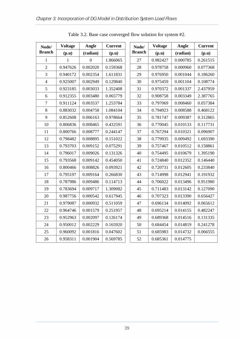
Chapter 3: Incorporation of DG Model in Distribution System Load Flows
39
Table 3.2. Base case converged flow solution for system #2.
Node/ Branch
Voltage Angle Current
Node/ Branch
Voltage Angle Current (p.u) (radian) (p.u) (p.u) (radian) (p.u)
1 1 0 1.866065 27 0.982427 0.000785 0.261515 2 0.947626 0.002020 0.159368 28 0.978758 0.000960 0.077368 3 0.940172 0.002354 1.611831 29 0.976950 0.001044 0.186260 4 0.925007 0.002949 0.129840 30 0.975459 0.001104 0.108774 5 0.923185 0.003033 1.352408 31 0.970372 0.001337 2.437959 6 0.912355 0.003480 0.065779 32 0.908758 0.003349 2.387765 7 0.911124 0.003537 1.253784 33 0.797069 0.008460 0.057384 8 0.883032 0.004758 1.084104 34 0.794923 0.008588 0.468122 9 0.852608 0.006163 0.978664 35 0.781747 0.009387 0.312865 10 0.806836 0.008465 0.432591 36 0.770045 0.010133 0.117731 11 0.800766 0.008777 0.244147 37 0.767294 0.010321 0.096907 12 0.798482 0.008895 0.151022 38 0.779935 0.009492 1.693390 13 0.793703 0.009152 0.075291 39 0.757467 0.010512 0.158861 14 0.796017 0.009026 0.131326 40 0.754495 0.010679 1.395190 15 0.793568 0.009142 0.454050 41 0.724840 0.012352 0.146440 16 0.800466 0.008826 0.093921 42 0.720731 0.012605 0.233840 17 0.795197 0.009164 0.266830 43 0.714998 0.012941 0.191932 18 0.787986 0.009486 0.114713 44 0.706022 0.013496 0.951980 19 0.783694 0.009717 1.309082 45 0.711483 0.013142 0.127090 20 0.987756 0.000542 0.617945 46 0.707323 0.013390 0.656427 21 0.979087 0.000932 0.511059 47 0.696134 0.014092 0.065612 22 0.964746 0.001579 0.251957 48 0.695214 0.014155 0.482247 23 0.952963 0.002097 0.126174 49 0.689368 0.014516 0.131335 24 0.950012 0.002229 0.165920 50 0.684454 0.014819 0.241278 25 0.960092 0.001816 0.047602 51 0.685983 0.014732 0.066555 26 0.958311 0.001904 0.569785 52 0.685361 0.014775

Chapter 3: Incorporation of DG Model in Distribution System Load Flows
40
3.10 SUMMARY
In this chapter, a simple distribution system load flow approaches has been formulated.
The Bus Injection to Branch Current (BIBC) matrix and Branch Current
to Node voltage (BCBV) matrix are the main part of this approaches. This two matrix make
the relation between the current injections to branch current and branch current to node
voltage. The matrix formation makes the load flow calculation very easy. The incorporation
of DG, capacitor bank and OLTTC into the load flow is much simple due to these calculation
is basically based on matrix addition, subtraction or multiplication. Also the satisfactory
result is obtained from the load flow approaches which is conducted on two different
radial distribution systems. With the definition of this load flow of radial distribution
networks, the highly required foundation has been ready to work in the area of
distributed generator allocation problem in radial distribution networks.
41
CHAPTER-4
OPTIMAL DG ALLOCATION USING GENETIC
ALGORITHM
4.1 INTRODUCTION
Optimization is a process by which we try to find out the best solution from set of available
alternative. In DG allocation problem, DG locations and sizes must be optimize in such a way
that it give most economical, efficient, technically sound distribution system. In general
distribution system have many nodes and it is very hard to find out the optimal DG location
and size by hand. There are numerous optimization approaches used in the literature. In most
of the current works, population based evolutionary algorithms are used as optimization
approaches (i.e. particle swarm optimization (PSO) [26-29], evolutionary programming [25],
genetic algorithm (GA) [20-25], etc.). In the project work genetic algorithm is used as the
solution strategy.
4.2 GENETIC ALGORITHM
Genetic Algorithms (GAs) are versatile exploratory hunt processes focused around the
evolutionary ideas of characteristic choice and genetics. A genetic algorithm is
a heuristically guided random search technique that concurrently evaluates
thousands of postulated solutions. Biased random selection and mixing of the
evaluated searches is then carried out in order to progress towards better solutions.
The coding and manipulation of search data is based upon the operation of genetic
DNA and the selection process is derived from Darwin’s survival of the fittest’.
Search data are usually coded as binary strings called chromosomes, which
collectively form populations. Evaluation is carried out over the whole population
and involves the application of, often complex ‘fitness’ functions to the string of
values (genes) within each chromosome. Typically, mixing involves recombining

Chapter 4: Optimal Distributed Generator Allocation Using Genetic Algorithm
42
the data that are held in two chromosomes that are selected from the whole
population.
Evolutionary computing was introduced in the 1960s by I. Rechenberg in his work
"Evolution strategies". His idea was then developed by other researchers. Genetic
Algorithms (GAs) were invented by John Holland at the University of Michigan.
This lead to Holland's book "Adaptation in Natural and Artificial Networks"
published in 1975. The goals of their research have been twofold: (1) to abstract
and rigorously explain the adaptive processes of natural networks and (2) to design
artificial networks software that retains the important mechanisms of natural networks.
The central theme of research on genetic algorithms has been ronodetness, the
balance between efficiency and efficacy necessary for survival in many different
environments. In 1992 John Koza has used genetic algorithm to evolve programs to
perform certain tasks. He called this method "Genetic Programming" (GP).
4.2.1 GAs vs Conventional Algorithms
Genetic Algorithms are different from normal optimization and search methods in four ways:
1. GAs work with coding of the parameter set, not the parameters themselves.
2. GAs search from a population of points, not a single point.
3. GAs use payoff (objective function) information, not derivatives or other auxiliary
knowledge.
4. GAs use probabilistic transition rules, not deterministic rules.
4.2.2 Genetic Algorithm Description
The genetic algorithm is a search algorithm that iteratively transforms a set (called a
population) of mathematical objects (typically fixed-length binary character strings), each
with an associated fitness value, into a new population of offspring objects using the
Darwinian principle of natural selection and using operations such as crossover (sexual
recombination) and mutation[75].
Chapter 4: Optimal Distributed Generator Allocation Using Genetic Algorithm
43
Algorithm begins with a set of solutions (represented by chromosomes) called
population. Solutions from one population are taken and used to form a new population.
This is motivated by a hope, that the new population will be better than
the old one. Solutions which are then selected to form new solutions (offspring) are
selected according to their fitness - the more suitable they are the more chances they
have to reproduce. This is repeated until some condition is satisfied.
The space of all feasible solutions (the set of solutions among which the desired
solution resides) is called search space (also state space). Each point in the search
space represents one possible solution. Each possible solution can be "marked" by
its value (or fitness) for the problem. With GA we look for the best solution among
a number of possible solutions. The problem is that the search can be very
complicated. One may not know where to look for a solution or where to start.
There are many methods one can use for finding a suitable solution, but these
methods do not necessarily provide the best solution.
A simple genetic algorithm that yields good results in many practical problems is composed
of three operators:
Reproduction: This operator is an artificial version of natural selection based on Darwinian
survival of the fittest among string creatures. Reproduction operator can be implemented in
algorithmic form in a number of ways.
Crossover: It occurs after reproduction or selection. It creates two new population or strings
from two existing ones by genetically recombining randomly chosen parts formed by
randomly chosen crossover point.
Mutation: It is the occasional random alteration of the value of a string position. Mutation
creates a new string by altering value of existing string.
Fitness function: A typical genetic algorithm requires two things to be defined: (1) a genetic
representation of solutions, (2) a fitness function to evaluate them. The fitness function is
defined over the genetic representation and measures the quality of the represented solution.
The fitness function is always problem dependent. Once we had the genetic representation
and the fitness function defined, GA proceeds to initialize a population of solutions
Chapter 4: Optimal Distributed Generator Allocation Using Genetic Algorithm
44
randomly, then improve it through repetitive application of mutation, crossover, and
selection operators.
4.2.3 Parameters of GA
There are two basic parameters of GA - crossover probability and mutation probability. Other
parameters include population size etc.
Crossover probability is how often crossover will be performed. If there is no
crossover, offspring are exact copies of parents. If there is crossover, offspring are
made from parts of both parent's chromosome. If crossover probability is 100%, then
all offspring are made by crossover. If it is 0%, whole new generation is made from
exact copies of chromosomes from old population. Crossover is made in hope that
new chromosomes will contain good parts of old chromosomes and therefore the
new chromosomes will be better.
Mutation probability is how often parts of chromosome will be mutated. If there is
no mutation, offspring are generated immediately after crossover (or directly copied)
without any change. If mutation is performed, one or more parts of a chromosome
are changed. If mutation probability is 100%, whole chromosome is changed, if it is
0%, nothing is changed. Mutation generally prevents the GA from falling into local
extremes. Mutation should not occur very often, because then GA will in fact change
to random search.
Population size is how many chromosomes are in population (in one generation). If there
are too few chromosomes, GA have few possibilities to perform crossover and only a small
part of search space is explored. On the other hand, if there are too many chromosomes,
GA slows down.
Chapter 4: Optimal Distributed Generator Allocation Using Genetic Algorithm
45
4.2.4 Algorithm of Basic GA
Step 1: Generate random population of 휂 chromosomes.
Step 2: Evaluate the objective function 휓(푥)and fitness 푓(휓) of each chromosome x in
the population
Step 3: Select the pairs of chromosome as parents from the population with giving a
priority that the better fitness parents will get highest chance to be selected in the
matting pool.
Step 4: According to the matting pool parents are crossed over with a crossover probability
and generate the offspring.
Step 5: Now the crossed offspring are mutated with a mutation probability where the
offspring locus are change slightly.
Step 6: Consider the mutate offspring as a new population and use it for the next
generation.
Step 7: If the solution satisfied the end condition, then stop, and display the optmial
solution.
Step 8: Go to step 2
The standard procedure of GA is shown in flowchart as shown in Figure 4.1.

Chapter 4: Optimal Distributed Generator Allocation Using Genetic Algorithm
46
Figure 4.1. Flowchart for basic GA algorithms
STOP
Converged?
START
Generate Initial Population
Gen = 0;
휓(푥)
푓(휓) 휓(푥);
Apply Crossover on the parent’s chromosome to Generate Offspring;
Mutate the Offspring’s Function and Evaluate Fitness Value of Each Offspring’s;
Select the parent’s chromosome in Pool from Initial Population by using Selection strategy;
Gen = Gen + 1;
From New Population = Solutions in the Pool (Selected by R.W. Selection) + Offspring’s (Generated by Crossover and Mutation);
Initial Population = New Population;
No
Yes

Chapter 4: Optimal Distributed Generator Allocation Using Genetic Algorithm
47
4.2.5 Applications of GA
Problems which give off an impression of being especially suitable for result by hereditary
calculations (genetic algorithms) incorporate timetabling and scheduling issues, and numerous
planning programming bundles are focused around GAs. GAs have likewise been connected
to engineering. Genetic algorithms are regularly connected as a methodology to take care of
global optimization problems. When in doubt of thumb genetic algorithms may be valuable in
issue areas that have a complex fitness landscape as mixing, i.e., mutation in consolidation
with crossover, is intended to move the populace far from local optima that a conventional
‘hill climbing’ algorithm may get stuck in. Since GAs are mainly used in optimization
and give outstanding performance, GAs are treated as function optimiser. But there are many
other ways to view genetic algorithms in different areas such as:
• GAs as problem solvers
• GAs as challenging technical puzzle
• GAs as basis for competent machine learning
• GAs as computational model of innovation and creativity
• GAs as computational model of other innovating networks
• GAs as guiding philosophy
Genetic algorithms have been used for difficult problems (such as NP-hard problems),
for machine learning and also for evolving simple programs. They have been also used for
some art, for evolving pictures and music. Some of the applications of GAs are:
• Nonlinear dynamical networks - predicting, data analysis
• Designing neural networks, both architecture and weights
• Robot trajectory
• Evolving LISP programs (genetic programming)
• Strategy planning
• Finding shape of protein molecules
• Signal Processing
• TSP and sequence scheduling
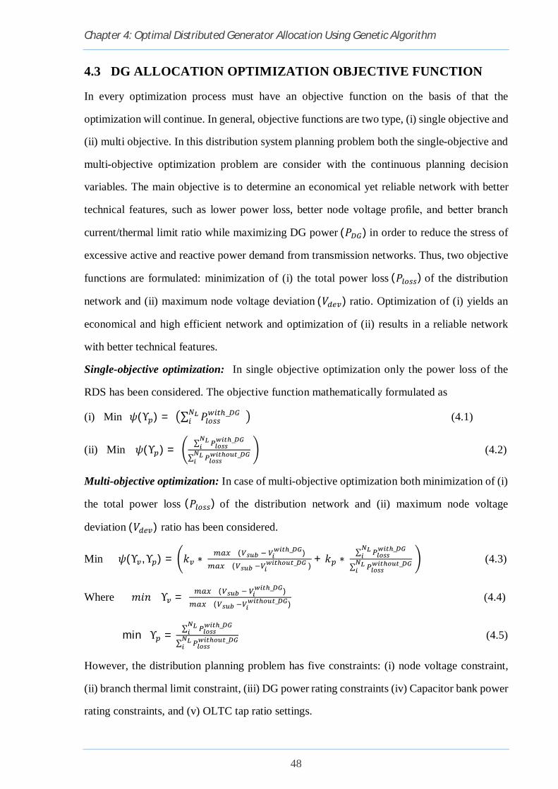
Chapter 4: Optimal Distributed Generator Allocation Using Genetic Algorithm
48
4.3 DG ALLOCATION OPTIMIZATION OBJECTIVE FUNCTION
In every optimization process must have an objective function on the basis of that the
optimization will continue. In general, objective functions are two type, (i) single objective and
(ii) multi objective. In this distribution system planning problem both the single-objective and
multi-objective optimization problem are consider with the continuous planning decision
variables. The main objective is to determine an economical yet reliable network with better
technical features, such as lower power loss, better node voltage profile, and better branch
current/thermal limit ratio while maximizing DG power (푃 )in order to reduce the stress of
excessive active and reactive power demand from transmission networks. Thus, two objective
functions are formulated: minimization of (i) the total power loss(푃 )of the distribution
network and (ii) maximum node voltage deviation(푉 ) ratio. Optimization of (i) yields an
economical and high efficient network and optimization of (ii) results in a reliable network
with better technical features.
Single-objective optimization: In single objective optimization only the power loss of the
RDS has been considered. The objective function mathematically formulated as
(i) Min휓(Υ ) = ∑ 푃 _ (4.1)
(ii) Min 휓(Υ ) = ∑ _
∑ _ (4.2)
Multi-objective optimization: In case of multi-objective optimization both minimization of (i)
the total power loss (푃 )of the distribution network and (ii) maximum node voltage
deviation(푉 ) ratio has been considered.
Min 휓(Υ ,Υ ) = 푘 ∗ ( _ )( _ )
+ 푘 ∗ ∑ _
∑ _ (4.3)
Where 푚푖푛Υ = ( _ )( _ )
(4.4)
min Υ =∑ _
∑ _ (4.5)
However, the distribution planning problem has five constraints: (i) node voltage constraint,
(ii) branch thermal limit constraint, (iii) DG power rating constraints (iv) Capacitor bank power
rating constraints, and (v) OLTC tap ratio settings.

Chapter 4: Optimal Distributed Generator Allocation Using Genetic Algorithm
49
Networks constraints:
a) All node voltage limits
푣 ≤ 푣 ≤ 푣 ∀푖 = 푁 (4.6)
b) Thermal limits
퐼 _ ≤ 퐼 _ _ ∀푖 = 푁 (4.7)
c) DG power limits
푃 ≤ 푃 _ ≤ 푃 ∀푖 = 푁 (4.8)
d) Capacitor bank power limits
푄 ≤ 푄 _ ≤ 푄 ∀푖 = 푁 (4.9)
e) Transformer tap setting limits
훼 ≤ 훼 ≤ 훼 ∀푖 = 푁 (4.10)
4.4 BASIC GA OPTIMIZATION FOR DG ALLOCATION
The main objective of optimization is to identifying the sizing and location of a sets of DG to
be introduced in to the distribution system. In this distribution system planning problem
optimization is done by genetic algorithm to determine an economical yet reliable network
with better technical features, such as lower power loss, better node voltage profile, and better
branch current/thermal limit ratio while maximizing DG power (푃 )in order to reduce the
stress of excessive active and reactive power demand from transmission networks. Previously
discussed a GA is an iterative procedure which begins with an initial population mainly which
randomly generated. There are several different encoding strategy for the initial population
which is depend upon the problem to be optimize. Objective function and fitness are calculated
for each and every chromosome of the population. On the basis of evaluated fitness functions
of the population, a set of chromosome is selected for the matting pool by the selection
operators. The selection operator select the chromosome in such a way that the chromosome
participate in the matting pool has better average fitness then that of initial population while
maintaining the same number of population in the matting pool. The crossover and mutation
operator are applied on the selected chromosome to generate new offerings. These process is
repeated iteratively, as the iteration progress, in most of the cases the process find the

Chapter 4: Optimal Distributed Generator Allocation Using Genetic Algorithm
50
improvement in solutions (i.e. offspring have better fitness then parents) and optimal solution
is obtained. With the above description, a simple Genetic Algorithm for DG allocation
problem is discussed in details as follow:
4.4.1 Coding Scheme
The success of the GA structure will lies on the coding scheme. In genetic algorithm coding
can be done by two different method (i) binary coding scheme and (ii) real number coding
schemes. In the study the practical coding scheme is selected for optimization process and
applied in the both radial distribution networks.
In this work, both the radial distribution system have one potential nodes. And all others nodes
are the load nodes. So, DG can be incorporate in any load node available in the network except
potential node. Also it is applicable for capacitor bank incorporation. But in case of OLTC, it
can be incorporate at any branch or in between two adjacent node of the networks.
So, in practical encoding of chromosome the location for DG and capacitor bank can be
randomly selected from any node except potential node, and for OLTC can be selected
randomly from any branch available in the network. The flexibility for selection of location
and size/settings for DG, OLTC and capacitor bank is given for better optimization.
4.4.2 Initialization
Initialization is the generation of initial population. Here, the initial population is generated
randomly which contains three optimization variables (i.e. locations and rating/settings and
number of DG or OLTC or Capacitor Bank). The generated value for all decision variable is
randomly generated. The DGs of different sizes (kW ratings) and CB of different sizes (kVAR
ratings) to be install at the load nodes except to the substation buss. The population size,
generation size, cross over probability, mutation probability effects the efficiency and
performance of the algorithm. Initially in the study it considered randomly some numerical
value. But for better performance of optimization later stage it is found out by multi run
process with different values of optimization parameters. For easy calculation in the study
minimum three and maximum decision variable is considered in one chromosome together
(OLTC with DG or Capacitor Bank).

Chapter 4: Optimal Distributed Generator Allocation Using Genetic Algorithm
51
Encoding of chromosome:
In the study total three decision variable had been considered for each DG optimization, OLTC
optimization, and Capacitor bank optimization as shown below.
Now in case of DG optimization:
1. Number of DG have to be consider in a string.
2. The node number of the networks where DG is to be connected/placed.
3. Corresponding DG power rating.
푁 휌 휌 휌 휌 --- 휌 Ρ Ρ Ρ Ρ Ρ -- Ρ
Number of DG ← DG Locations → ← DG Ratings →
Now in case of Capacitor Bank optimization:
1. Number of CB have to be consider in a string.
2. The node number of the networks where CB is to be connected/placed.
3. Corresponding CB rating.
푁 휌 휌 휌 휌 --- 휌 Φ Φ Φ Φ Φ -- Φ
Number of CB ← Capacitor Bank
Locations → ← Capacitor Bank Ratings →
Now in case of OLTC optimization:
1. Number of OLTC had to be consider in a string.
2. Branch number of the networks where the OLTC is to be connected/placed.
3. Corresponding tap setting will be applied to the OLTC.
푁 휌 휌 휌 휌 --- 휌 α α α α α -- α
Number of
OLTC ← OLTC Locations → ← OLT C Settings →
These are the optimization variable and it is used in a single chromosome structure. Now
combination of these three is shown below.
푁 휌 … 휌 Ρ … Ρ 푁 휌 … 휌 Φ … Φ 푁 휌 … 휌 α … α
← DG → ← Capacitor Bank → ← OLT C →

Chapter 4: Optimal Distributed Generator Allocation Using Genetic Algorithm
52
4.4.3 Fitness Function
After generating population of required size the corresponding load flow solution with
optimization variable (i.e. DG, OLTC or capacitor bank) for different cases is run to evaluate
the objective function 휓 Υ ,Υ 표푟휓(Υ ) for each and every chromosome. The load flow
solution, evaluation of objective function and fitness function is repeated for all the strings in
the population. The procedure to determine the fitness function ‘푓(휓) ’ is very much
application oriented. It is directly associated with the objective function value in the
optimization problem. In the distributed generator placement problem, the objective function
is the minimization of cost function. After calculating the objective function, the fitness
function 푓(휓) is calculated using two different method as given below:
In initial stage of the project, for single-objective optimization, the fitness of the each
chromosome is calculated using the method of Roulette Wheel and selection of chromosome
for next generation is selected directly from it. The method is mathematically formulated as
given below:
푓(휓) = ( )∑ ( )
푖 = 1,2,3 … … 푝표푝푠푖푧푒 (4.11)
But later stage of project, fitness function in both single-objective as well as multi objective
optimization is totally different from previous one and which gives the better performance of
the optimization. Also this fitness function take a major part into the adaptive or improved
genetic algorithm where the crossover and mutation probability is directly depend upon the
fitness function of population.
푓(휓) = ( , )
푖 = 1,2,3 … … 푝표푝푠푖푧푒 (4.12)
4.4.4 Reproduction
The first genetic algorithm operator is reproduction. This determines which chromosome of
the current population will be participate in matting pool to create the next generation
population. So, basically this operator is known as the selection operator for breeding. This
is done by using some biased random selection approach. Hence parents are randomly
selected or chosen from the current population in such a way that the ‘best’ strings in the
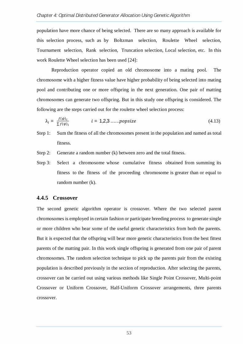
Chapter 4: Optimal Distributed Generator Allocation Using Genetic Algorithm
53
population have more chance of being selected. There are so many approach is available for
this selection process, such as by Boltzman selection, Roulette Wheel selection,
Tournament selection, Rank selection, Truncation selection, Local selection, etc. In this
work Roulette Wheel selection has been used [24]:
Reproduction operator copied an old chromosome into a mating pool. The
chromosome with a higher fitness value have higher probability of being selected into mating
pool and contributing one or more offspring in the next generation. One pair of matting
chromosomes can generate two offspring. But in this study one offspring is considered. The
following are the steps carried out for the roulette wheel selection process:
λ = ( )∑ ( )
푖 = 1,2,3 … … 푝표푝푠푖푧푒 (4.13)
Step 1: Sum the fitness of all the chromosomes present in the population and named as total
fitness.
Step 2: Generate a random number (k) between zero and the total fitness.
Step 3: Select a chromosome whose cumulative fitness obtained from summing its
fitness to the fitness of the proceeding chromosome is greater than or equal to
random number (k).
4.4.5 Crossover
The second genetic algorithm operator is crossover. Where the two selected parent
chromosomes is employed in certain fashion or participate breeding process to generate single
or more children who bear some of the useful genetic characteristics from both the parents.
But it is expected that the offspring will bear more genetic characteristics from the best fittest
parents of the matting pair. In this work single offspring is generated from one pair of parent
chromosomes. The random selection technique to pick up the parents pair from the existing
population is described previously in the section of reproduction. After selecting the parents,
crossover can be carried out using various methods like Single Point Crossover, Multi-point
Crossover or Uniform Crossover, Half-Uniform Crossover arrangements, three parents
crossover.

Chapter 4: Optimal Distributed Generator Allocation Using Genetic Algorithm
54
In the present work two parents uniform crossover is used. This is illustrated in the following
example. Let Parent1 and Parent2 be the two parents selected randomly for crossover. Assume
the strings parent1 and parent2 as given below and, a universal crossover site is selected by
generating a random number of 0 to 1 with giving same priority (0.5) for both the parents.
Bothe the parents are shown in different colour for better understanding.
Parent1 푁 _ 휌 휌 휌 휌 휌 -- 휌 Ρ Ρ Ρ Ρ Ρ -- Ρ Cross(>0.5) Y N N Y N Y Y N N Y N Y N
Parent2 푁 _ 휌 휌 휌 휌 휌 -- 휌 Ρ Ρ Ρ Ρ Ρ -- Ρ
Number of DG ← DG Locations → ← DG Ratings →
For illustration the string length is taken as randomly, but in the thesis work string length
depends upon the maximum number of DG, OLTC and capacitor bank to be considered into
RDS.
Let the crossover site is randomly position. Then single children is generated as below.
Offspring 푁 _ 휌 휌 휌 휌 휌 -- 휌 Ρ Ρ Ρ Ρ Ρ -- Ρ
Number of DG ← DG Locations → ← DG Ratings →
It is seen that each crossover resulted in the children. In order to control crossover rate also
there is a parameter known as “Crossover Probability(Ω )” which is discuss details in later
stage. This probability is used as a decision variable before performing the crossover. This
probability is known as the crossover rate. Crossover probability lies in the range of 0 - 1. The
following steps are carried out to perform crossover.
Step 1: Form a matting pool of parent’s chromosomes by randomly selection method. The
size of matting pool must be same with the population size.
Step 2: Select one of the parent’s pair from the matting pool and generate random number
between 0 and 1.
Step 3: Set a crossover probability ‘Ω ’.
Step 4: If the randomly generated number is greater than crossover probability ‘Ω ’ cross
over will not occur and the offspring will contained only one parent chromosome.
The offspring can be selected by two different method (i) best fitness parent
among the parent pair and (ii) the chromosome belongs the same location or

Chapter 4: Optimal Distributed Generator Allocation Using Genetic Algorithm
55
number of the selected parent’s pair location or number in the population and
matting pool respectively.
Step 5: If the randomly generated number is less than crossover probability ‘Ω ’ than
crossover takes place and a single offspring is generate.
4.4.6 Mutation
Selection and crossover efficiently search and recombine the surviving chromosomes.
Mutation is a genetic operator which is capable of creation new genetic material in the
population to maintain the population diversity. It is nothing but random alteration of
chromosome variable or optimize variable (i.e. DG and capacitor bank locations, size, and
OLTC locations and settings). The following example illustrates the mutation operation.
Let Mutation site is at 4th position of the string.
Crossed Offspring:
Offspring 푁 _ 휌 휌 휌 휌 휌 -- 휌 Ρ Ρ Ρ Ρ Ρ -- Ρ
Mutate(>0.5) N N N Y N N N N N N N Y N
Number of DG ← DG Locations → ← DG Ratings →
Offspring after mutation
Offspring 푁 _ 휌 휌 휌 휌 휌 -- 휌 Ρ Ρ Ρ Ρ Ρ -- Ρ
Number of DG ← DG Locations → ← DG Ratings →
In the above illustration after getting the mutation site, a random value is generated from
corresponding allocated value is placed at the mutation site showing (xx). Hence GA can come
to better solution by using mutation. Mutation occurs during evolution according to a user-
definable mutation probability. This probability should be set low. If it is set too high, the
search will turn into a primitive random search. Generally the mutation probability ‘(Ω )’
must be below 5%. The following steps to be carried out to perform the mutation:
Step 1: Generate random number between 0 and 1.
Step 2: Set a mutation probability ‘(Ω )’.
Chapter 4: Optimal Distributed Generator Allocation Using Genetic Algorithm
56
Step 3: If the randomly generated number is less than mutation probability ‘(Ω )’ than
mutation is executed on the off-springs which generated after the crossover
operation.
4.4.7 Elitism
When creating a new population by crossover and mutation, there are
chances that the best chromosome is lost. Elitism is the name of the method that
first copies the best chromosome (or few best chromosomes) to the new population.
The rest of the population is constructed according to GA. Elitism can rapidly
increase the performance of GA, because it prevents a loss of the best found
solution.
4.4.8 Genetic Control Parameter Selection:
Genetic parameters are the entities that help to tune the performance of the genetic algorithm.
The selection of values for these parameters plays an important role in obtaining an optimal
solution. There are some general guidelines, which could be followed to arrive at an optimal
values for these parameters. There are two basic parameters of GA - crossover probability
and mutation probability. Other parameters include population size, maximum generation etc.
Population size: It is the number of chromosomes consist in population or in one generation.
Genetic algorithm give very poor performance with a very small populations, because the
population provides an insufficient amount of sample for gating the most optimal result and
only a small search space is explored. A large population is more likely to contain
representative from a large number of hyper planes. Hence GAs can perform a more
informed search. As a result, a large population discourages premature convergence to
suboptimal solution. On the other hand, a large population requires more evaluations per
generation, possibly resulting in an unacceptably slow rate of convergence.
Crossover probability (훀풄) : the higher the crossover rate, the more quickly new
chromosome are introduced into the population. If the crossover rate is too high, high
performance chromosome are discarded faster than the selection can produced improvements.
If the crossover rate is low, the search may deteriorate due to the lower exploration rate.
Chapter 4: Optimal Distributed Generator Allocation Using Genetic Algorithm
57
Crossover is made in hope that new chromosomes will contain best parts of parent’s
chromosomes and therefore the child chromosomes will be better in the sense of fitness.
Mutation probability(훀풎): If there is no mutation, offspring are generated immediately
after crossover (or directly copied) without any change. Mutation generally prevents the GA
from falling into local extremes. A low level of mutation serves to prevent any given bit
position from getting stuck to a single value or local extremes. Also mutation should not occur
very often, because then GA will in fact change to random search.
4.5 ALGORITHM FOR DG ALLOCATION
The general layout of the Loss minimization and the Genetic calculation for DGs allocation
issue is discussed in the previous sections. A set of steps have been indicated beneath to tackle
the DGs allocation problem:
Step 1: Read the distribution networks line data and bus data (i.e. branch impedance, real
and reactive power of each load node.) and specify the DG parameters.
Step 2: Run load flow of distribution networks, and save the all node voltage and all branch
current magnitudes of the networks and total power loss.
Step 3: Set GEN = 0
Step 4: Randomly generate the initial population. Where the chromosomes are representing
the randomly generated values of tap number, tap positions, tap settings, DGs
number, DG positions, and DG active power value, etc.
Step 5: Decode the initial population and update the load-data and bus-data (i.e. tap settings,
and DG ratings.) to the networks matrixes according to their respective positions.
Step 6: Run the load flow of distribution networks with updated system data. Also calculate
total power loss for each population.
Step 7: Evaluate the objective function and the fitness value for each and every
chromosome.
Step 8: Perform the elitism and save the population.
Step 9: GEN = GEN + 1
Chapter 4: Optimal Distributed Generator Allocation Using Genetic Algorithm
58
Step 10: form the matting pool from initial population by using Roulette Wheel Selection
procedure.
Step 11: Perform crossover on the each matting chromosome pair and generate one offspring
from each parent’s chromosome pair;
Step 12: Perform mutation on the offspring produced by the crossover operation.
Step 13: Decode the set of offspring and and determine the DG location and size for each
chromosome.
Step 14: Run foal flow for each offspring to determine the objective function and assign
fitness to each offspring.
Step 15: Perform the elitism and select the 휂 best chromosome from the current
population and the offspring’s. Replace the initial population by selected best
population and use it for the next generation.
Step 16: Go to step 9, till the solution converges.
Step 17: STOP
The standard optimization procedure of DG allocation problem is shown in flowchart as
shown in Figure 4.2.

Chapter 4: Optimal Distributed Generator Allocation Using Genetic Algorithm
59
Figure 4.2. Flowchart of DG allocation with basic genetic algorithm
START
Input system data and specify GA parameters, population size, and maximum generation (휂 ,퐺푒푛 );
Randomly generate initial population;
Gen = 1;
Decode the initial population and determine the DG location and size for each chromosome;
Perform Load Flow for each Chromosome to determine objective function and assign fitness to each Chromosome;
Select the Chromosomes in the current population by using Roulette Wheel Selection;
Apply Crossover and Mutation operators to obtain the set of offspring from the current population;
Perform Load Flow for each offspring to determine objective function and assign fitness to each offspring;
Decode the set of offspring and and determine the DG location and size for each chromosome;
Select 휂 number of best chromosomes from the current population and from the set of offspring;
Gen = Gen + 1;
Converged?
The best chromosome of the current population represents the optimal solution;
STOP
Yes
No
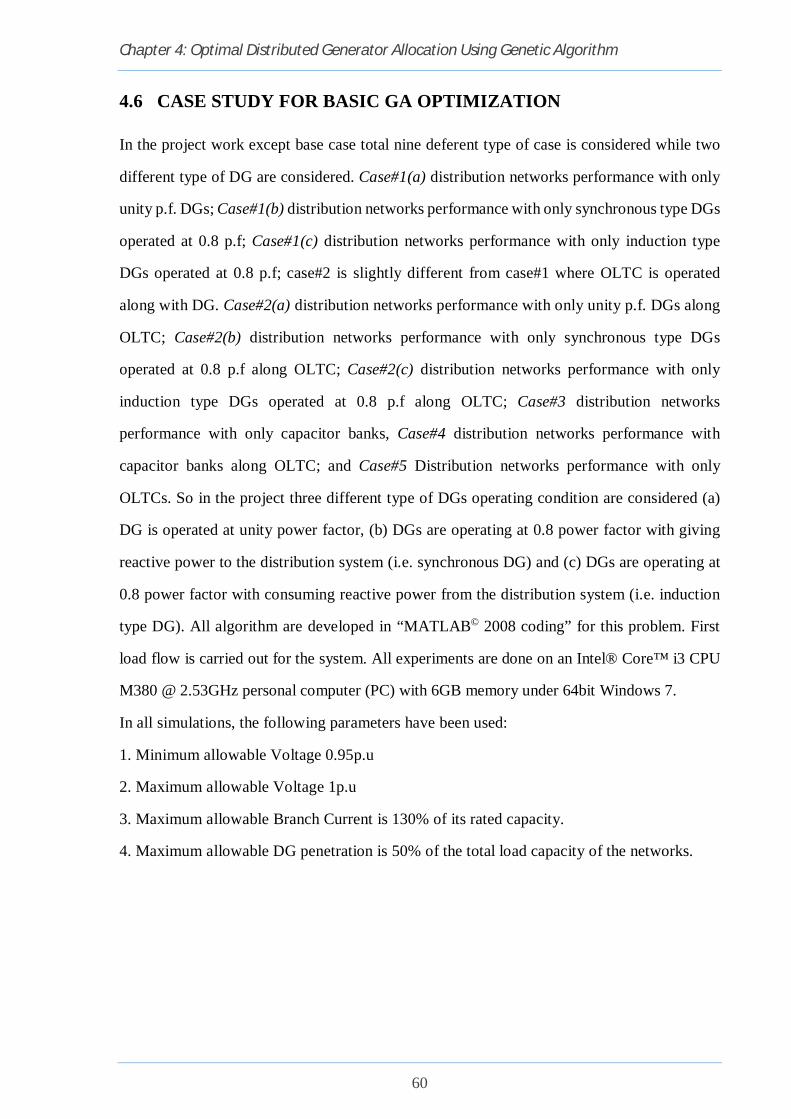
Chapter 4: Optimal Distributed Generator Allocation Using Genetic Algorithm
60
4.6 CASE STUDY FOR BASIC GA OPTIMIZATION
In the project work except base case total nine deferent type of case is considered while two
different type of DG are considered. Case#1(a) distribution networks performance with only
unity p.f. DGs; Case#1(b) distribution networks performance with only synchronous type DGs
operated at 0.8 p.f; Case#1(c) distribution networks performance with only induction type
DGs operated at 0.8 p.f; case#2 is slightly different from case#1 where OLTC is operated
along with DG. Case#2(a) distribution networks performance with only unity p.f. DGs along
OLTC; Case#2(b) distribution networks performance with only synchronous type DGs
operated at 0.8 p.f along OLTC; Case#2(c) distribution networks performance with only
induction type DGs operated at 0.8 p.f along OLTC; Case#3 distribution networks
performance with only capacitor banks, Case#4 distribution networks performance with
capacitor banks along OLTC; and Case#5 Distribution networks performance with only
OLTCs. So in the project three different type of DGs operating condition are considered (a)
DG is operated at unity power factor, (b) DGs are operating at 0.8 power factor with giving
reactive power to the distribution system (i.e. synchronous DG) and (c) DGs are operating at
0.8 power factor with consuming reactive power from the distribution system (i.e. induction
type DG). All algorithm are developed in “MATLAB© 2008 coding” for this problem. First
load flow is carried out for the system. All experiments are done on an Intel® Core™ i3 CPU
M380 @ 2.53GHz personal computer (PC) with 6GB memory under 64bit Windows 7.
In all simulations, the following parameters have been used:
1. Minimum allowable Voltage 0.95p.u
2. Maximum allowable Voltage 1p.u
3. Maximum allowable Branch Current is 130% of its rated capacity.
4. Maximum allowable DG penetration is 50% of the total load capacity of the networks.
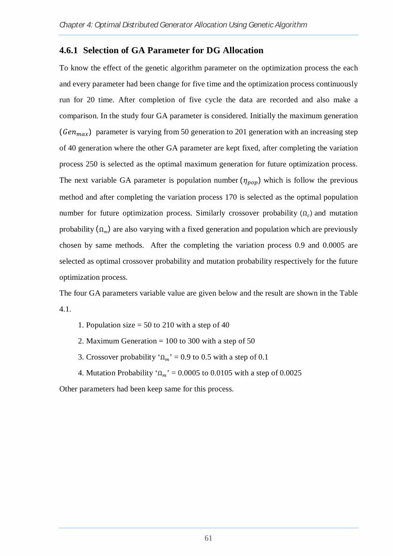
Chapter 4: Optimal Distributed Generator Allocation Using Genetic Algorithm
61
4.6.1 Selection of GA Parameter for DG Allocation
To know the effect of the genetic algorithm parameter on the optimization process the each
and every parameter had been change for five time and the optimization process continuously
run for 20 time. After completion of five cycle the data are recorded and also make a
comparison. In the study four GA parameter is considered. Initially the maximum generation
(퐺푒푛 ) parameter is varying from 50 generation to 201 generation with an increasing step
of 40 generation where the other GA parameter are kept fixed, after completing the variation
process 250 is selected as the optimal maximum generation for future optimization process.
The next variable GA parameter is population number(휂 ) which is follow the previous
method and after completing the variation process 170 is selected as the optimal population
number for future optimization process. Similarly crossover probability (Ω )and mutation
probability(Ω푚) are also varying with a fixed generation and population which are previously
chosen by same methods. After the completing the variation process 0.9 and 0.0005 are
selected as optimal crossover probability and mutation probability respectively for the future
optimization process.
The four GA parameters variable value are given below and the result are shown in the Table
4.1.
1. Population size = 50 to 210 with a step of 40
2. Maximum Generation = 100 to 300 with a step of 50
3. Crossover probability ‘Ω ’ = 0.9 to 0.5 with a step of 0.1
4. Mutation Probability ‘Ω ’ = 0.0005 to 0.0105 with a step of 0.0025
Other parameters had been keep same for this process.

Chapter 4: Optimal Distributed Generator Allocation Using Genetic Algorithm
62
Table 4.1. GA parameter selection with system#1
Network parameter
Tap settings limit = 0.95 to 1.05; Maximum DG power = 500kW;
Minimum DG power =50 kW; DG penetration limit = 1500 kW;
Maximum no. of Tap = 20; Maximum no. of DG = 10;
Maximum allowable line Current = 40%; Minimum Voltage Settings = 0.9 p.u.;
Maximum run for GA optimization = 20; Maximum iteration for load flow = 300;
Accuracy label in load flow= 10-9
푮풆풏풎풂풙 휼풑풐풑 훀풄 훀풎 Elite Power Loss (Kw) Average Power
Loss (Kw) Minimum Fitness
Minimum Mean Value
Standard Deviation
Mean Value
Standard Deviation
Minimum Value
Standard Deviation
100 150 200 250 300
50 50 50 50 50
0.9 0.9 0.9 0.9 0.9
0.0005 0.0005 0.0005 0.0005 0.0005
37.578 41.239 42.772 41.646 43.761
67.657 63.135 65.236 64.614 63.556
13.303 11.565 10.937 11.864 10.445
105.400 98.418 100.310 94.891 93.982
15.244 14.176 13.830 15.717 14.801
0.00215 0.00166 0.00238 0.00288 0.00295
0.00121 0.00090 0.00098 0.00132 0.00093
250 250 250 250 250
50 90
130 170 210
0.9 0.9 0.9 0.9 0.9
0.0005 0.0005 0.0005 0.0005 0.0005
39.196 25.791 30.651 25.929 24.989
62.471 43.281 44.001 37.601 34.079
13.611 9.639 8.253 7.099 3.092
93.504 74.661 76.431 67.873 66.828
18.618 14.123 13.146 11.139 6.5806
0.00245 0.00107 0.00093 0.00046 0.00046
0.00144 0.00041 0.00015 0.00018 7.6e-005
250 250 250 250 250
170 170 170 170 170
0.9 0.8 0.7 0.6 0.5
0.0005 0.0005 0.0005 0.0005 0.0005
29.274 25.182 33.308 30.371 39.648
38.83 42.943 45.763 49.829 54.160
6.876 10.020 7.274 10.536 9.254
70.846 79.116 83.174 87.064 94.515
10.391 17.193 12.648 16.106 12.711
0.00057 0.00063 0.00065 0.00069 0.00072
0.00020 0.00017 0.00016 0.00013 0.00018
250 250 250 250 250
170 170 170 170 170
0.9 0.9 0.9 0.9 0.9
0.0005 0.0030 0.0055 0.0080 0.0105
28.943 23.910 27.296 22.930 17.176
36.208 35.894 35.100 35.909 31.753
5.065 8.548 6.909 7.964 5.681
66.532 65.074 64.449 64.879 60.003
9.7136 14.814 11.366 11.783 9.5657
0.00062 0.00054 0.00058 0.00063 0.00056
0.00011 0.00015 9.6e-005 0.00011 0.00010
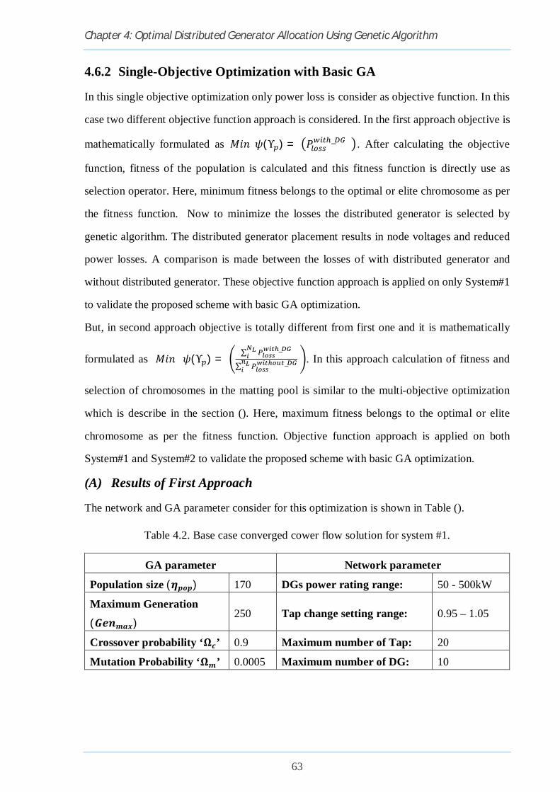
Chapter 4: Optimal Distributed Generator Allocation Using Genetic Algorithm
63
4.6.2 Single-Objective Optimization with Basic GA
In this single objective optimization only power loss is consider as objective function. In this
case two different objective function approach is considered. In the first approach objective is
mathematically formulated as 푀푖푛휓(Υ ) = 푃 _ . After calculating the objective
function, fitness of the population is calculated and this fitness function is directly use as
selection operator. Here, minimum fitness belongs to the optimal or elite chromosome as per
the fitness function. Now to minimize the losses the distributed generator is selected by
genetic algorithm. The distributed generator placement results in node voltages and reduced
power losses. A comparison is made between the losses of with distributed generator and
without distributed generator. These objective function approach is applied on only System#1
to validate the proposed scheme with basic GA optimization.
But, in second approach objective is totally different from first one and it is mathematically
formulated as푀푖푛휓(Υ ) = ∑ _
∑ _ . In this approach calculation of fitness and
selection of chromosomes in the matting pool is similar to the multi-objective optimization
which is describe in the section (). Here, maximum fitness belongs to the optimal or elite
chromosome as per the fitness function. Objective function approach is applied on both
System#1 and System#2 to validate the proposed scheme with basic GA optimization.
(A) Results of First Approach
The network and GA parameter consider for this optimization is shown in Table ().
Table 4.2. Base case converged cower flow solution for system #1.
GA parameter Network parameter
Population size(휼풑풐풑) 170 DGs power rating range: 50 - 500kW
Maximum Generation
(푮풆풏풎풂풙) 250 Tap change setting range: 0.95 – 1.05
Crossover probability ‘훀풄’ 0.9 Maximum number of Tap: 20
Mutation Probability ‘훀풎’ 0.0005 Maximum number of DG: 10
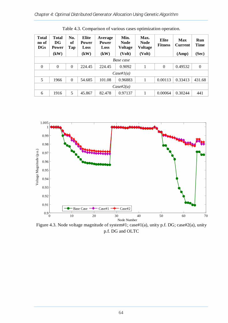
Chapter 4: Optimal Distributed Generator Allocation Using Genetic Algorithm
64
Table 4.3. Comparison of various cases optimization operation.
Total no of DGs
Total DG
Power
No. of
Tap
Elite Power Loss
Average Power Loss
Min. Node
Voltage
Max. Node
Voltage
Elite Fitness
Max Current
Run Time
(kW) (kW) (kW) (Volt) (Volt) (Amp) (Sec) Base case
0 0 0 224.45 224.45 0.9092 1 0 0.49532 0 Case#1(a)
5 1966 0 54.685 101.08 0.96883 1 0.00113 0.33413 431.68 Case#2(a)
6 1916 5 45.867 82.478 0.97137 1 0.00064 0.30244 441
Figure 4.3. Node voltage magnitude of system#1; case#1(a), unity p.f. DG; case#2(a), unity
p.f. DG and OLTC
0 10 20 30 40 50 60 700.9
0.91
0.92
0.93
0.94
0.95
0.96
0.97
0.98
0.99
11.005
Node Number
Vol
tage
Mag
nitu
de (p
.u.)
Base Case Case#1 Case#2

Chapter 4: Optimal Distributed Generator Allocation Using Genetic Algorithm
65
Figure 4.4. Branch current magnitude of system#1; case#1(a), unity p.f. DG; case#2(a), unity
p.f. DG and OLTC
0 10 20 30 40 50 60 700
0.05
0.1
0.15
0.2
0.25
0.3
0.35
0.4
0.45
0.5
Node Number
Curr
ent M
agni
tude
(p.u
.)
Base Case Case#1 Case#2
Figure 4.5. Generation wise variation of average and minimum power loss of system#1 for
case#1(a) unity p.f. DG
0 50 100 150 200 25050
100
150
200
Generation
Pow
er L
oss (
kW)
Elite Average

Chapter 4: Optimal Distributed Generator Allocation Using Genetic Algorithm
66
Figure 4.6. Generation wise variation of average and minimum power loss of system#1 for
case#2(a) unity p.f. DG and OLTC
0 50 100 150 200 25020
40
60
80
100
120
140
160
180
200
Pow
er L
oss (
kW)
Generation
Elite Average
Figure 4.7. Comparison of average and minimum power loss in different cases; case#1(a),
unity p.f. DG; case#2(a), unity p.f. DG and OLTC
0 50 100 150 200 250
40
60
80
100
120
140
160
180
200
Generation
Pow
er L
oss (
kW)
Case#1: EliteCase#1: AverageCase#2: EliteCase#2: Average

Chapter 4: Optimal Distributed Generator Allocation Using Genetic Algorithm
67
Table 4.4. Converged Power Flow Solution of case#1(a); case#1(a), unity p.f. DG
Node/ Branch
Voltage Angle Current Node/ Branch
Voltage Angle Current (p.u) (radian) (p.u) (p.u) (radian) (p.u)
1 1 0 0.33413244 36 0.999933 -2.06E-05 0.019432 2 0.9999735 -5.84E-06 0.33413244 37 0.999761 -0.00013 0.016238 3 0.9999471 -1.17E-05 0.30251104 38 0.999603 -0.00017 0.016238 4 0.9998746 -2.48E-05 0.20853272 39 0.999557 -0.00019 0.013296 5 0.9993968 0.0001323 0.20853272 40 0.999555 -0.00019 0.010354 6 0.9953527 0.0036349 0.20822975 41 0.998857 -0.00038 0.010198 7 0.9911637 0.0073101 0.20392146 42 0.998565 -0.00046 0.010198 8 0.990184 0.0081982 0.19176452 43 0.998526 -0.00047 0.009459 9 0.9897113 0.0086662 0.09547209 44 0.998518 -0.00047 0.009459
10 0.9847748 0.0101099 0.09203603 45 0.998419 -0.00051 0.00473 11 0.9836639 0.0103954 0.0693878 46 0.998419 -0.00051 0.104766 12 0.9805428 0.0112947 0.04418254 47 0.999825 -5.64E-05 0.104766 13 0.9776548 0.0120857 0.04318975 48 0.998579 -0.00084 0.095045 14 0.974793 0.0128718 0.04219404 49 0.994734 -0.00327 0.047536 15 0.9719599 0.0136532 0.04219404 50 0.994189 -0.00361 0.005444 16 0.9714335 0.0137988 0.03658378 51 0.990149 0.008203 0.000454 17 0.9705642 0.0140395 0.02943985 52 0.99014 0.008206 0.12738 18 0.9705555 0.014042 0.02230417 53 0.989243 0.010161 0.127105 19 0.9700964 0.014187 0.02230417 54 0.988707 0.011906 0.1257 20 0.9698013 0.0142804 0.02218428 55 0.988027 0.014341 0.124497 21 0.9693253 0.0144313 0.00775709 56 0.987417 0.016746 0.124497 22 0.9693185 0.0144334 0.00710225 57 0.986166 0.029887 0.124497 23 0.9692476 0.0144561 0.00710225 58 0.985613 0.036376 0.124497 24 0.9690932 0.0145056 0.00355158 59 0.98542 0.038894 0.113671 25 0.9689228 0.014554 0.00355158 60 0.984732 0.041714 0.120885 26 0.968854 0.0145761 0.00177581 61 0.981589 0.044692 0.050929 27 0.9688347 0.0145823 0.01124013 62 0.981793 0.044979 0.020997 28 0.9999402 -1.61E-05 0.00804314 63 0.981722 0.045183 0.035853 29 0.9998685 -6.14E-05 0.00484593 64 0.979958 0.045452 0.007394 30 0.9997473 -2.43E-05 0.00484593 65 0.979425 0.045533 0.004515 31 0.999726 -1.78E-05 0.00484593 66 0.983608 0.010415 0.002257 32 0.9996191 1.50E-05 0.00484593 67 0.983607 0.010415 0.007021 33 0.9993629 9.22E-05 0.00312438 68 0.980217 0.011398 0.00351 34 0.9990274 0.0001944 0.00072186 69 0.980216 0.011398 35 0.99896 0.0002129 0.02262588

Chapter 4: Optimal Distributed Generator Allocation Using Genetic Algorithm
68
Table 4.5. Converged Power Flow Solution of case#2(a); case#2(a), unity p.f. DG and OLTC
Node/ Branch
Voltage Angle Current Node/ Branch
Voltage Angle Current (p.u) (radian) (p.u) (p.u) (radian) (p.u)
1 1 0 0.30243529 36 0.999939 -2.40E-05 0.019432 2 0.9999766 -7.50E-06 0.30243529 37 0.999768 -0.00014 0.016238 3 0.9999533 -1.50E-05 0.27137821 38 0.999609 -0.00018 0.016238 4 0.9998897 -3.29E-05 0.17303922 39 0.999563 -0.00019 0.013296 5 0.9994811 5.19E-05 0.17303922 40 0.999561 -0.00019 0.010354 6 0.9958186 0.0025579 0.17272026 41 0.998864 -0.00038 0.010198 7 0.9920205 0.0051847 0.16813566 42 0.998571 -0.00046 0.010198 8 0.9911346 0.0058175 0.15510393 43 0.998532 -0.00047 0.009459 9 0.9907117 0.0061488 0.08447434 44 0.998524 -0.00048 0.009459 10 0.9872132 0.002859 0.09110796 45 0.998426 -0.00051 0.00473 11 0.9861106 0.0031288 0.0685247 46 0.998425 -0.00051 0.104783 12 0.9830159 0.003969 0.04340238 47 0.99984 -6.45E-05 0.104783 13 0.9801619 0.0046764 0.04241291 48 0.998401 -0.00111 0.095062 14 0.9773343 0.0053773 0.04142059 49 0.994555 -0.00354 0.047544 15 0.9745356 0.006072 0.04142059 50 0.99401 -0.00389 0.005439 16 0.973966 0.0060883 0.03648832 51 0.9911 0.005823 0.000454 17 0.973099 0.0063277 0.029363 52 0.99109 0.005826 0.169748 18 0.9730902 0.0063301 0.02224591 53 0.989469 0.008067 0.1263 19 0.9726323 0.0064744 0.02224591 54 0.988871 0.009779 0.124781 20 0.972338 0.0065673 0.02212633 55 0.988103 0.012167 0.123472 21 0.9718633 0.0067174 0.00773682 56 0.987406 0.014526 0.123472 22 0.9718565 0.0067196 0.00708369 57 0.985659 0.027503 0.121986 23 0.9717858 0.0067422 0.00708369 58 0.984392 0.033759 0.121986 24 0.9716318 0.0067913 0.0035423 59 0.983922 0.036191 0.115129 25 0.9714619 0.0068395 0.0035423 60 0.982657 0.038843 0.117693 26 0.9713932 0.0068615 0.00177117 61 0.97987 0.042021 0.05422 27 0.9713739 0.0068676 0.01019768 62 0.980096 0.042319 0.028284 28 0.9999477 -1.99E-05 0.00706337 63 0.980173 0.042601 0.035909 29 0.9998959 -7.34E-05 0.00402867 64 0.978406 0.042871 0.007406 30 0.9997914 -8.67E-05 0.00402867 65 0.977872 0.042952 0.004504 31 0.9997714 -1.01E-04 0.00484571 66 0.986055 0.003148 0.002252 32 0.9996645 -6.80E-05 0.00484571 67 0.986054 0.003148 0.007003 33 0.9994083 9.25E-06 0.00312424 68 0.982691 0.004072 0.003502 34 0.9990728 0.0001114 0.00072183 69 0.98269 0.004072 35 0.9990054 0.00013 0.02262574

Chapter 4: Optimal Distributed Generator Allocation Using Genetic Algorithm
69
Multiple Run Optimal Solution for first approach:
Optimization result for 10 run:
Table 4.6. Optimal Power Flow Solutions for 10 run.
Total no of DGs
Total DG
Power
No. of
Tap
Elite Power Loss
Average Power Loss
Min. Node
Voltage
Max. Node
Voltage
Elite Fitness
Max Current
(kW) (kW) (kW) (Volt) (Volt) (Amp) Case#2(a), impact of unity p.f. DG and OLTC into the system
5 2098 19 26.401 48.900 0.97368 1 0.00060 0.25723 4 2188 18 20.598 44.606 0.97412 1 0.00064 0.21012 4 2125 14 31.470 62.851 0.9117 1 0.00057 0.26984 4 2156 13 30.714 67.830 0.9182 1 0.00050 0.26116 4 2177 19 18.748 53.117 0.97327 1 0.00061 0.24902 4 2184 19 23.821 51.535 0.97315 1 0.00066 0.25722 3 2027 16 26.650 56.750 0.97354 1 0.00049 0.26048 3 2047 17 43.911 67.370 0.96820 1 0.00092 0.31372 4 2091 17 19.364 51.390 0.97436 1 0.00052 0.23411 3 1962 18 29.133 60.029 0.97104 1 0.00071 0.22457
Base case 0 0 0 224.45 224.45 0.9092 1 0 0.49532
Figure 4.8. Run wise variation of minimum and average power losses
1 2 3 4 5 6 7 8 9 100
10
20
30
40
50
60
70
80
90
100
Number of Run
Pow
er L
oss i
n kW
Elite Average

Chapter 4: Optimal Distributed Generator Allocation Using Genetic Algorithm
70
(B) Results of Second Approach
Table 4.7. Comparison of various cases optimization operation.
System
Total no of DGs
Total DG
Power
No. of
Tap
Elite Power Loss
Average Power Loss
Min. Node
Voltage
Max. Node
Voltage
Elite Fitness
Max Current
(kW) (kW) (kW) (Volt) (Volt) (Amp)
System#1
Base case 0 0 0 224.45 224.45 0.90920 1 0 0.49532
Case#1(a), impact of unity p.f. DG into the system 5 1957 0 55.895 56.024 0.96877 1 0.80101 0.33487
Case#2(a), impact of unity p.f. DG and OLTC into the system 5 1957 13 21.698 22.051 0.97401 1 0.91204 0.26307
System#2
Base case 0 0 0 887.057 887.057 0.68445 1 0 2.4380
Case#1(a), impact of unity p.f. DG into the system 6 1951 0 118.63 119.05 0.90012 1 0.88204 1.3091
Case#2(a), impact of unity p.f. DG and OLTC into the system 6 1950 15 110.01 110.57 0.88322 1 0.88966 1.3036
Figure 4.9. Node voltage magnitude of system#1; case#1(a), unity p.f. DG; case#2(a), unity
p.f. DG and OLTC
0 10 20 30 40 50 60 700.9
0.91
0.92
0.93
0.94
0.95
0.96
0.97
0.98
0.99
11.005
Node Number
Vol
tage
Mag
nitu
de (p
.u.)
Base Case Case#1 Case#2

Chapter 4: Optimal Distributed Generator Allocation Using Genetic Algorithm
71
Figure 4.10. Branch current magnitude of system#1; case#1(a), unity p.f. DG; case#2(a),
unity p.f. DG and OLTC
0 10 20 30 40 50 60 700
0.05
0.1
0.15
0.2
0.25
0.3
0.35
0.4
0.45
0.5
Node Number
Curr
ent M
agni
tude
(p.u
.)
Base Case Case#1 Case#2
Figure 4.11. Comparison of average and minimum power loss in different cases; case#1(a),
unity p.f. DG; case#2(a), unity p.f. DG and OLTC
0 50 100 150 200 25020
40
60
80
100
120
140
160
180
200
Generation
Pow
er L
oss (
kW)
Case#1: EliteCase#1: AverageCase#2: EliteCase#2: Average

Chapter 4: Optimal Distributed Generator Allocation Using Genetic Algorithm
72
Figure 4.12. Comparison of average and minimum objective function in different cases;
case#1(a), unity p.f. DG; case#2(a), unity p.f. DG and OLTC
0 50 100 150 200 2500
0.1
0.2
0.3
0.4
0.5
0.6
0.7
0.8
0.9
Generation
Obj
ect F
unct
ion
Case#1: EliteCase#1: AverageCase#2: EliteCase#2: Average

Chapter 4: Optimal Distributed Generator Allocation Using Genetic Algorithm
73
Multiple Run Optimal Solution of Second Approach:
Optimization result for 10 run:
Table 4.8. Converged Power Flow Solution for 10 run.
Total no of DGs
Total DG
Power
No. of
Tap
Elite Power Loss
Average Power Loss
Min. Node
Voltage
Max. Node
Voltage
Elite Fitness
Max Current
(kW) (kW) (kW) (Volt) (Volt) (Amp) Case#2(a), impact of unity p.f. DG and OLTC into the system
5 2328 10 21.616 30.115 0.98810 1 0.88288 0.23486 5 2330 10 28.663 28.937 0.98182 1 0.85925 0.27798 5 2318 8 23.824 23.831 0.97705 1 0.84798 0.28470 5 2317 10 21.582 25.638 0.98137 1 0.6331 0.27641 6 2330 10 33.842 33.936 0.98741 1 0.87373 0.27789 5 2329 7 28.126 32.139 0.98053 1 0.84841 0.28801 5 2330 9 31.495 34.354 0.98644 1 0.87361 0.22488 5 2328 10 31.254 31.687 0.98503 1 0.86817 0.27552 6 2330 10 33.399 33.553 0.98654 1 0.87084 0.27644 6 2321 9 26.028 26.062 0.98875 1 0.89304 0.21810
Base case 0 0 0 224.45 224.45 0.9092 1 0 0.49532
Figure 4.13. Run wise variation of minimum and average power losses
1 2 3 4 5 6 7 8 9 100
5
10
15
20
25
30
35
Number of Run
Pow
er L
oss i
n kW
Elite Average

Chapter 4: Optimal Distributed Generator Allocation Using Genetic Algorithm
74
4.6.3 Multi-Objective Optimization with Basic GA
The main objective of this multi-objective optimization is to determine an economical and
reliable network with better technical features, such as lower power loss, better node voltage
profile, and better branch current/thermal limit ratio. Thus, two objective function are
formulated as (i) the total power loss(푃 )of the distribution network and (ii) maximum node
voltage deviation(푉 ) ratio. These multi-objective function approach is applied on both
System#1 and System#2 to validate the proposed scheme with basic GA optimization. The GA
parameter and network constraints consider for this optimization is shown in Table (4.9).
Table 4.9. GA and network parameters considered for the optimization process
GA parameter Network parameter
Population size(휂 ) 100 DGs power rating range (푃 ): 50 - 600kW
Maximum Generation (퐺푒푛 ) 300 Tap change setting
range(훼): System#1 = 0.94 – 1.06 System#2 = 0.90 – 1.10
Crossover probability ‘Ω ’ 0.9 Maximum number of Tap: System#1 = 10 System#2 = 20
Mutation Probability ‘Ω ’ 0.0005 Maximum number of DG/Capacitor bank: 10
Figure 4.14. Variation of optimal active and reactive power loss of system#1
Base 1(a) 1(b) 1(c) 2(a) 2(b) 2(c) 3 4 50
50
100
150
200
250
Cases
Pow
er L
oss i
n kW
/kV
AR
Active Power Reactive Power

Chapter 4: Optimal Distributed Generator Allocation Using Genetic Algorithm
75
Figure 4.15. Variation of optimal active and reactive power loss of system#2
Base 1(a) 1(b) 1(c) 2(a) 2(b) 2(c) 3 4 50
100
200
300
400
500
600
700
800
900
Cases
Pow
er L
oss
in k
W/k
VA
R
Active Power Reactive Power
Figure 4.16. Variation of minimum node voltage of system#1 and system#2
case#1(a), unity p.f. DG; case#1(b), DG operating at 0.8 p.f. leading; case#1(c), DG operating at 0.8 p.f. lagging; case#2(a), unity p.f. DG with OLCT; case#2(b), DG operating at 0.8 p.f. leading with OLTC.; case#2(c), DG operating at 0.8 p.f. lagging with OLTC; case#3, capacitor bank; case#4, capacitor bank with OLTC; case#5, only OLTC.
Base 1(a) 1(b) 1(c) 2(a) 2(b) 2(c) 3 4 50.5
0.55
0.6
0.65
0.7
0.75
0.8
0.85
0.9
0.95
1
Cases
Vol
tage
Mag
nitu
de in
p.u
.
System#1 System#2

Chapter 4: Optimal Distributed Generator Allocation Using Genetic Algorithm
76
Multiple Run Optimized Load Flow Solution
Figure 4.17. Variation of maximum branch current of system#1 and system#2
case#1(a), unity p.f. DG; case#1(b), DG operating at 0.8 p.f. leading; case#1(c), DG operating at 0.8 p.f. lagging; case#2(a), unity p.f. DG with OLCT; case#2(b), DG operating at 0.8 p.f. leading with OLTC.; case#2(c), DG operating at 0.8 p.f. lagging with OLTC; case#3, capacitor bank; case#4, capacitor bank with OLTC; case#5, only OLTC.
Base 1(a) 1(b) 1(c) 2(a) 2(b) 2(c) 3 4 50
0.5
1
1.5
2
2.5
Cases
Curr
ent M
agni
tude
in p
.u.
System#1 System#2
Table 4.10. Multiple run solution for different case with system#2
Case
Minimum Active Power Loss (kW)
Average Active Power Loss (kW) Minimum Voltage Average Objective
Function
Elite Mean Value
Standard Deviation
Mean Value
Standard Deviation
Minimum Value
Mean Value
Standard Deviation
Mean Value
Standard Deviation
1(a) 57.263 72.875 9.117 73.33 9.305 0.93084 0.94027 0.004699 0.13639 0.005399
1(b) 65.103 69.613 2.589 69.71 2.544 0.94078 0.94993 0.002367 0.11877 0.004685
1(c) 507.9 556.56 21.330 562.73 18.613 0.81280 0.83233 0.006841 0.58308 0.006356
2(a) 42.994 58.747 10.267 59.195 10.329 0.92600 0.94250 0.004800 0.12490 0.006800
2(b) 57.371 62.750 3.362 63.085 3.281 0.94750 0.95270 0.001800 0.11090 0.004100
2(c) 469.96 510.137 20.057 515.82 17.268 0.80040 0.84240 0.010700 0.54080 0.012500
3 778.38 778.66 0.1555 778.69 0.1505 0.71868 0.71887 0.000117 0.88440 0.000254
4 716.52 722.59 3.329 722.88 3.647 0.78700 0.79550 0.001600 0.79590 0.004300
5 799.21 807.65 4.518 807.83 4.452 0.72531 0.72784 0.001419 0.88668 0.004574

Chapter 4: Optimal Distributed Generator Allocation Using Genetic Algorithm
77
From the Figure 4.14 and Figure 4.15 shows that DG placement in the distribution system is
profitable. From the above result it can be concluded that the multi-objective optimization
give the better optimal result then the single-objective optimization. In this multi-objective
optimization, priority of each objective function can defined separately. In the case study the
priority for each objective function is same.
Table 4.11. Multi-objective optimization for different system with basic GA optimization
Different Cases
Different systems
No. of
DG
Total DG Power No.
of Tap
No. of
CB
Total CB Reactive Power (kW)
Optimal Active Power Loss (kW)
Optimal Reactive Power Loss
(kVAR)
Min. Node
Voltage (Volt)
Max Current (Amp) Active
Power (kW)
Reactive Power
(kVAR)
Base System # 1 - - - - - - 224.995 102.198 0.90919 0.49031 System # 2 - - - - - - 887.181 381.694 0.68442 2.43820
Case # 1 (a)
System # 1 6 2328.0 - - - - 58.796 25.465 0.98262 0.31404 System # 2 6 2323.0 - - - - 70.072 30.147 0.93635 1.30910
Case # 1 (b)
System # 1 6 1864.0 1398.0 - - - 12.18 10.486 0.98747 0.23480 System # 2 6 1858.4 1393.8 - - - 68.732 29.571 0.95001 1.30910
Case # 1 (c)
System # 1 4 1639.2 -1229.4 - - - 200.212 88.861 0.94072 0.46945 System # 2 7 1836.8 -1377.6 - - - 540.792 232.666 0.83178 2.18770
Case # 2 (a)
System # 1 5 2325.0 - 10 - - 35.003 15.000 0.98751 0.28087 System # 2 7 2322.0 - 19 - - 51.265 22.056 0.94570 1.30270
Case # 2 (b)
System # 1 6 1863.2 1397.4 9 - - 8.052 8.303 0.98946 0.21720 System # 2 6 1858.4 1393.8 19 - - 59.235 25.485 0.95292 1.30520
Case # 2 (c)
System # 1 3 1433.6 -1075.2 10 - - 161.553 71.863 0.94630 0.43166 System # 2 6 1854.4 -1390.8 15 - - 535.240 230.278 0.84044 2.05950
Case # 3 System # 1 - - - - 4 2329.0 130.231 56.850 0.94073 0.40015 System # 2 - - - - 5 2324.0 778.845 335.085 0.71878 2.24170
Case # 4 System # 1 - - - 8 4 2320.0 132.456 57.386 0.94586 0.39830 System # 2 - - - 19 5 2324.0 726.877 312.726 0.75302 2.14780
Case # 5 System # 1 - - - 10 - - 171.446 78.606 0.91679 0.43205 System # 2 - - - 20 - - 809.771 348.390 0.72612 2.30250

Chapter 4: Optimal Distributed Generator Allocation Using Genetic Algorithm
78
4.7 IMPROVED GENETIC ALGORITHM (IGA) OPTIMIZATION
The traditional crossover like partly matched crossover, order crossover and cycle crossover,
etc. and mutation would make some unfeasible solution to be created. In the traditional
crossover and mutation, crossover probability and mutation probability are not adaptive in
nature and which have no flexibility. For this reason when a basic GA optimization process
trapped in a local minima these crossover and mutation probability cannot emerge from the
local minima and GA optimization give a premature result. In the project study some different
type of crossover and mutation method is considered to resolve all this problem. Also an
adaptive crossover probability is proposed.
GA#1: In [76], based on the mechanism of biological DNA genetic information and evolution,
a modified genetic algorithm (MDNA-GA) is proposed. They proposed a new mutation named
adaptive mutation probability which is dynamically adjusted by considering a measure called
Diversity Index (DI). It is defined to indicate the premature convergence degree of the
population.
푓 = ∑ 푓 (4.14)
Accordingly [22], the mutation probability is changed according to the following equation:
Ω = 0.5 ∗ (1 − ) ∗ 퐷퐼 (4.15)
GA#2: In [77], an Improved Genetic Algorithm (IGA) is proposed. The self-adaptive process
have been employed for crossover and mutation probability in order to improve crossover and
mutation quality. The crossover probability and mutation probability is controlled by
evolutionary degree and is defined by Eq. (4.16) and (4.17).
Ω = 0.9 − 0.3 ∗ ,푓 ≥ 푓 (4.16a)
Ω = 0.9,푓 < 푓 (4.16b)
Ω = 0.1 − 0.099 ∗ ( ) ,푓 ≥ 푓 (4.17a)
Ω = 0.1,푓 < 푓 (4.17b)
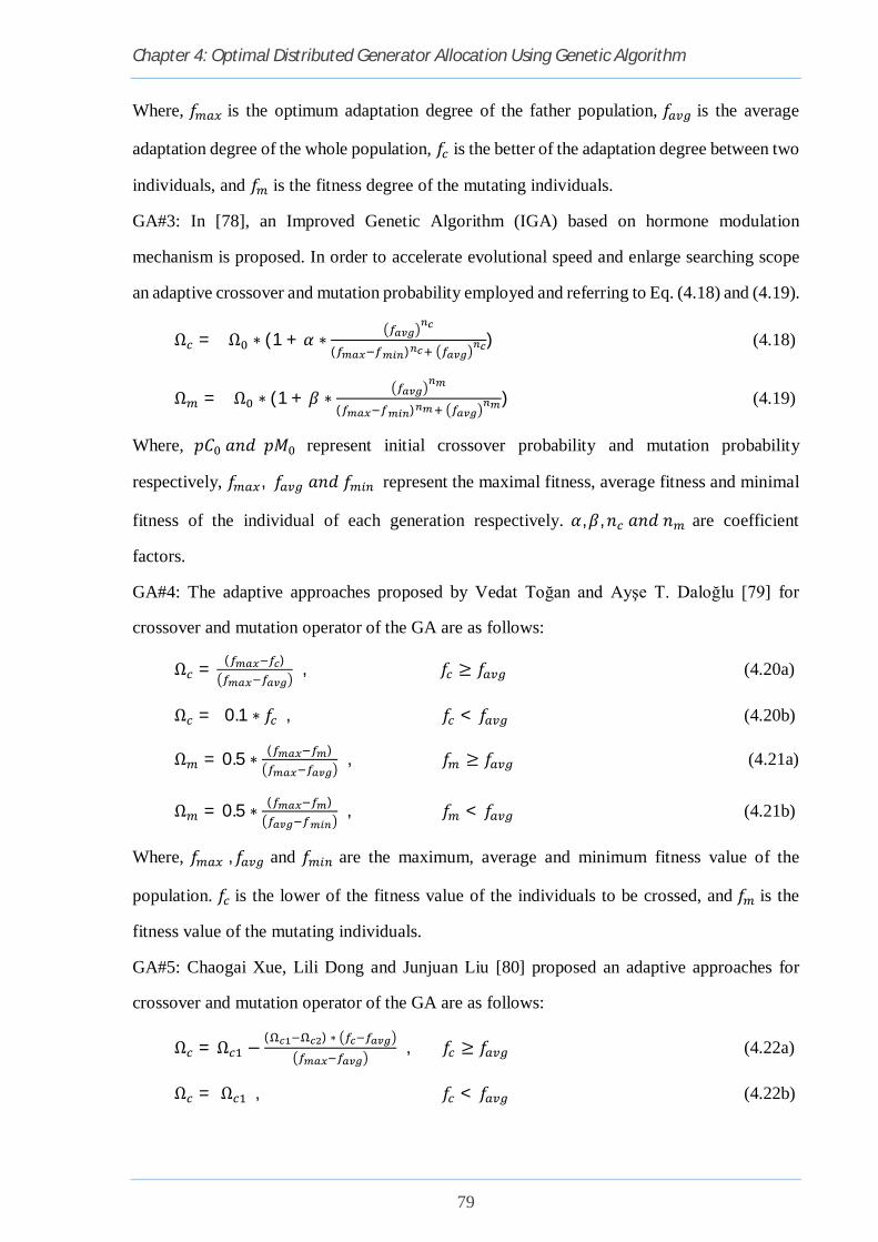
Chapter 4: Optimal Distributed Generator Allocation Using Genetic Algorithm
79
Where, 푓 is the optimum adaptation degree of the father population, 푓 is the average
adaptation degree of the whole population, 푓 is the better of the adaptation degree between two
individuals, and 푓 is the fitness degree of the mutating individuals.
GA#3: In [78], an Improved Genetic Algorithm (IGA) based on hormone modulation
mechanism is proposed. In order to accelerate evolutional speed and enlarge searching scope
an adaptive crossover and mutation probability employed and referring to Eq. (4.18) and (4.19).
Ω = Ω ∗ (1 + 훼 ∗( )
) (4.18)
Ω = Ω ∗ (1 + 훽 ∗( )
) (4.19)
Where, 푝퐶 푎푛푑푝푀 represent initial crossover probability and mutation probability
respectively, 푓 , 푓 푎푛푑푓 represent the maximal fitness, average fitness and minimal
fitness of the individual of each generation respectively. 훼,훽, 푛 푎푛푑푛 are coefficient
factors.
GA#4: The adaptive approaches proposed by Vedat Toğan and Ayşe T. Daloğlu [79] for
crossover and mutation operator of the GA are as follows:
Ω = ( ) ,푓 ≥ 푓 (4.20a)
Ω = 0.1 ∗ 푓 ,푓 < 푓 (4.20b)
Ω = 0.5 ∗ ( ) , 푓 ≥ 푓 (4.21a)
Ω = 0.5 ∗ ( ) ,푓 < 푓 (4.21b)
Where, 푓 , 푓 and 푓 are the maximum, average and minimum fitness value of the
population. 푓 is the lower of the fitness value of the individuals to be crossed, and 푓 is the
fitness value of the mutating individuals.
GA#5: Chaogai Xue, Lili Dong and Junjuan Liu [80] proposed an adaptive approaches for
crossover and mutation operator of the GA are as follows:
Ω = Ω −( )∗ ,푓 ≥ 푓 (4.22a)
Ω = Ω ,푓 < 푓 (4.22b)

Chapter 4: Optimal Distributed Generator Allocation Using Genetic Algorithm
80
Ω = Ω −( )∗ ,푓 ≥ 푓 (4.23a)
Ω = Ω ,푓 < 푓 (4.23b)
Where, 푓 , 푓 and 푓 are the maximum, average and minimum fitness value of the
population. 푓 is the grater of the fitness value of the two individuals to be crossed, and 푓 is
the fitness value of the mutating individuals,푝퐶 , 푝퐶 and 푝푀 , 푝푀 are initial values for
calculating self-adaptive crossover and mutation probability respectively.
GA#7: combination of two different IGA approach. Adaptive crossover operator taken from
[76] and adaptive mutation operator taken from [79].
GA#8: combination of two different IGA approach. Adaptive crossover operator taken from
[76] and adaptive mutation operator taken from [77].
4.7.1 Algorithm of Adaptive GA
The algorithm of all adaptive genetic algorithm is same with the basic genetic algorithm. In
basic genetic algorithm the crossover and mutation GA parameters are initialize at the starting
of the program. But in the adaptive genetic algorithm the crossover and mutation parameter
are updated in every generation before the crossover and mutation is performed. Because the
parameter are adaptive in nature. The flowchart for the adaptive genetic algorithm is presented
below.
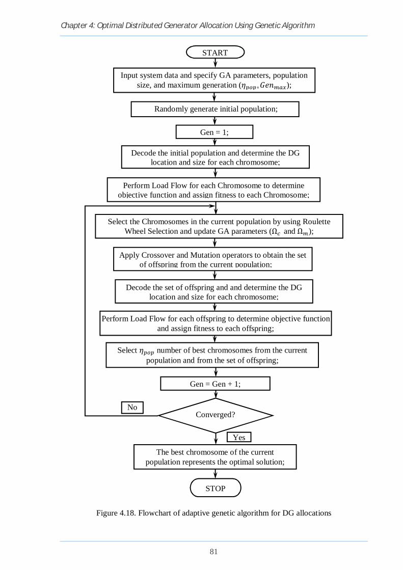
Chapter 4: Optimal Distributed Generator Allocation Using Genetic Algorithm
81
Figure 4.18. Flowchart of adaptive genetic algorithm for DG allocations
START
Input system data and specify GA parameters, population size, and maximum generation (휂 ,퐺푒푛 );
Randomly generate initial population;
Gen = 1;
Decode the initial population and determine the DG location and size for each chromosome;
Perform Load Flow for each Chromosome to determine objective function and assign fitness to each Chromosome;
Select the Chromosomes in the current population by using Roulette Wheel Selection and update GA parameters (Ω andΩ );
Apply Crossover and Mutation operators to obtain the set of offspring from the current population;
Perform Load Flow for each offspring to determine objective function and assign fitness to each offspring;
Decode the set of offspring and and determine the DG location and size for each chromosome;
Select 휂 number of best chromosomes from the current population and from the set of offspring;
Gen = Gen + 1;
Converged?
The best chromosome of the current population represents the optimal solution;
STOP
Yes
No
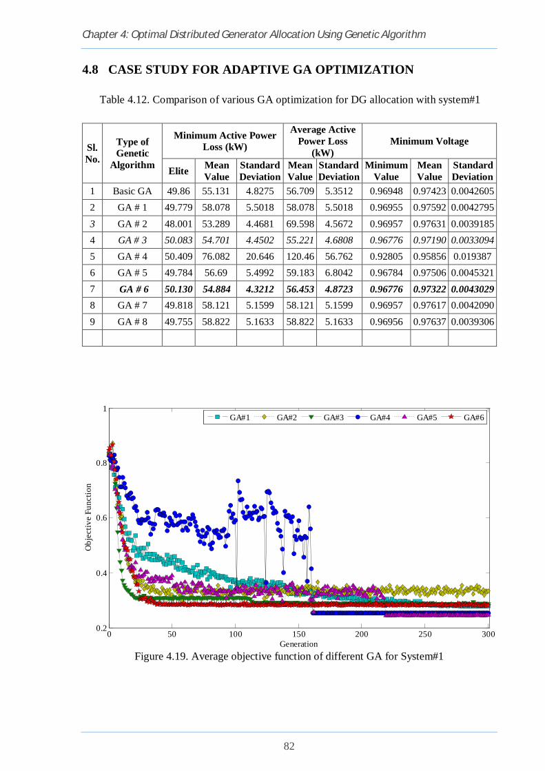
Chapter 4: Optimal Distributed Generator Allocation Using Genetic Algorithm
82
4.8 CASE STUDY FOR ADAPTIVE GA OPTIMIZATION
Table 4.12. Comparison of various GA optimization for DG allocation with system#1
Sl. No.
Type of Genetic
Algorithm
Minimum Active Power Loss (kW)
Average Active Power Loss
(kW) Minimum Voltage
Elite Mean Value
Standard Deviation
Mean Value
Standard Deviation
Minimum Value
Mean Value
Standard Deviation
1 Basic GA 49.86 55.131 4.8275 56.709 5.3512 0.96948 0.97423 0.0042605 2 GA # 1 49.779 58.078 5.5018 58.078 5.5018 0.96955 0.97592 0.0042795 3 GA # 2 48.001 53.289 4.4681 69.598 4.5672 0.96957 0.97631 0.0039185 4 GA # 3 50.083 54.701 4.4502 55.221 4.6808 0.96776 0.97190 0.0033094 5 GA # 4 50.409 76.082 20.646 120.46 56.762 0.92805 0.95856 0.019387 6 GA # 5 49.784 56.69 5.4992 59.183 6.8042 0.96784 0.97506 0.0045321 7 GA # 6 50.130 54.884 4.3212 56.453 4.8723 0.96776 0.97322 0.0043029 8 GA # 7 49.818 58.121 5.1599 58.121 5.1599 0.96957 0.97617 0.0042090 9 GA # 8 49.755 58.822 5.1633 58.822 5.1633 0.96956 0.97637 0.0039306
Figure 4.19. Average objective function of different GA for System#1
0 50 100 150 200 250 3000.2
0.4
0.6
0.8
1
Generation
Obj
ectiv
e Fu
nctio
n
GA#1 GA#2 GA#3 GA#4 GA#5 GA#6

Chapter 4: Optimal Distributed Generator Allocation Using Genetic Algorithm
83
The Table 4.12 and Figure 4.19 shows the results of various adaptive GA optimization
approaches. In this case study only case#1(a) is considered (i.e. installed DG are operated at
unity p.f. on the distribution systems). All the GA a give a well constricted result. But, some of
the GA give more satisfactory results (i.e. less standard dilation, low minimum power loss in
the generations, high minimum node voltage compare to other, etc.). The second objective
function gives the better performance with all the adaptive GA and particularly with basic GA
compare to first objective function approach. Though the basic GA have a quick convergence
criteria. Results shows that GA#3 have the best result among all of the GA previously proposed
by others though the GA is partially adaptive in nature. Table 4.12 is also contained the
proposed adaptive genetic algorithm results. It shows that the proposed adaptive GA gives the
most satisfactory and acceptable result among all the GA approach is considered in the study.
The proposed GA give the better result in all part of optimization (i.e. in case for minimum
voltage and power loss). The optimized result of GA#3 are discussed briefly in the section 4.8.1
and proposed GA are discussed letter stage of this thesis.
4.8.1 Case Study for Adaptive Ga#3 Optimization
Figure 4.20. Convergence of GA#3 for unity p.f. DG optimization with System#1
0 50 100 150 200 250 3000.1
0.2
0.3
0.4
0.5
0.6
0.7
0.8
Generation
Obj
ect F
unct
ion
EliteAverage

Chapter 4: Optimal Distributed Generator Allocation Using Genetic Algorithm
84
Figure 4.21. Adaptive crossover probability of GA#3 with System#2
0 50 100 150 200 250 3000.78
0.8
0.82
0.84
0.86
0.88
0.9
0.92
Generation
Cro
ssov
er P
roba
bilit
y
Figure 4.22. Adaptive mutation probability of GA#3 with System#2
0 50 100 150 200 250 3000.00108
0.0011
0.00112
0.00114
0.00116
0.00118
0.0012
0.00121
Generation
Mut
atio
n Pr
obab
ility

Chapter 4: Optimal Distributed Generator Allocation Using Genetic Algorithm
85
Figure 4.23. Node voltage magnitude of GA#3 for system#1 in different cases;
Figure 4.24. Active and Reactive power loss with injected DG and capacitor bank power rating.
case#1(a), unity p.f. DG; case#1(b), DG operating at 0.8 p.f. leading; case#1(c), DG operating at 0.8 p.f. lagging; case#2(a), unity p.f. DG with OLCT; case#2(b), DG operating at 0.8 p.f. leading with OLTC.; case#2(c), DG operating at 0.8 p.f. lagging with OLTC; case#3, capacitor bank; case#4, capacitor bank with OLTC; case#5, only OLTC.
0 10 20 30 40 50 60 700.9
0.92
0.94
0.96
0.98
1
Node Number
Vol
tage
Mag
nitu
de (p
.u.)
Base 1(a) 1(b) 1(c) 2(a) 2(b) 2(c) 3 4 5Case
base 1(a) 1(b) 1(c) 2(a) 2(b) 2(c) 3 4 50
500
1,000
1,500
2,000
2,500
Case
Pow
er in
W/V
AR
Active Loss Reactive Loss DG Active Rating DG Reactive Rating CB Rating

Chapter 4: Optimal Distributed Generator Allocation Using Genetic Algorithm
86
Figure 4.25. Node voltage magnitude of GA#3 for System#2
0 10 20 30 40 50 530.65
0.7
0.75
0.8
0.85
0.9
0.95
1
Node Number
Vol
tage
Mag
nitu
de (p
.u.)
Base 1(a) 1(b) 1(c) 2(a) 2(b) 2(c) 3 4 5
Case#
Figure 4.26. Node voltage magnitude of GA#3 for System#2;
case#1(a), unity p.f. DG; case#1(b), DG operating at 0.8 p.f. leading; case#1(c), DG operating at 0.8 p.f. lagging; case#2(a), unity p.f. DG with OLCT; case#2(b), DG operating at 0.8 p.f. leading with OLTC.; case#2(c), DG operating at 0.8 p.f. lagging with OLTC; case#3, capacitor bank; case#4, capacitor bank with OLTC; case#5, only OLTC.
0 10 20 30 40 50 530.65
0.7
0.75
0.8
0.85
0.9
0.95
1
Node Number
Vol
tage
Mag
nitu
de (p
.u.)
Base 1(b) 1(c) 2(b) 2(c) 3 4 5Case#
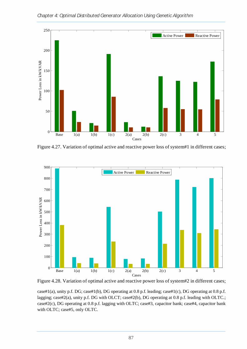
Chapter 4: Optimal Distributed Generator Allocation Using Genetic Algorithm
87
Figure 4.27. Variation of optimal active and reactive power loss of system#1 in different cases;
Base 1(a) 1(b) 1(c) 2(a) 2(b) 2(c) 3 4 50
50
100
150
200
250
Cases
Pow
er L
oss i
n kW
/kV
AR
Active Power Reactive Power
Figure 4.28. Variation of optimal active and reactive power loss of system#2 in different cases;
case#1(a), unity p.f. DG; case#1(b), DG operating at 0.8 p.f. leading; case#1(c), DG operating at 0.8 p.f. lagging; case#2(a), unity p.f. DG with OLCT; case#2(b), DG operating at 0.8 p.f. leading with OLTC.; case#2(c), DG operating at 0.8 p.f. lagging with OLTC; case#3, capacitor bank; case#4, capacitor bank with OLTC; case#5, only OLTC.
Base 1(a) 1(b) 1(c) 2(a) 2(b) 2(c) 3 4 50
100
200
300
400
500
600
700
800
900
Cases
Pow
er L
oss i
n kW
/kV
AR
Active Power Reactive Power

Chapter 4: Optimal Distributed Generator Allocation Using Genetic Algorithm
88
Table 4.13. Different case study for different system with GA#3 optimization
Different Cases
Different systems
No. of
DG
Total DG
Power
Total DG
Power No. of
Tap
No. of
CB
Total CB
Reactive Power
(kVAR)
Optimal Active Power Loss (kW)
Optimal Reactive Power Loss
(kVAR)
Min. Node
Voltage (Volt)
Max Current (Amp) Active
Power (kW)
Active Power (kW)
Base System # 1 - - - - - - 224.995 102.198 0.90919 0.49031 System # 2 - - - - - - 887.181 381.694 0.68442 2.43820
Case # 1 (a)
System # 1 4 2094.0 - - - - 50.978 23.547 0.96958 0.32700 System # 2 4 2094.0 - - - - 93.850 40.377 0.89538 1.30910
Case # 1 (b)
System # 1 4 1659.2 1244.4 - - - 20.710 14.538 0.97706 0.26130 System # 2 6 1674.4 1255.8 - - - 89.718 38.599 0.94084 1.30910
Case # 1 (c)
System # 1 3 1438.4 -1078.8 - - - 190.849 85.898 0.93630 0.46620 System # 2 5 1648.0 -1236.0 - - - 544.027 234.058 0.82427 2.09880
Case # 2 (a)
System # 1 5 2085.0 - 9 - - 23.267 10.286 0.98302 0.23862 System # 2 6 2091.0 - 20 - - 78.929 33.957 0.93245 1.30910
Case # 2 (b)
System # 1 5 1678.4 1258.8 10 - - 11.974 10.253 0.98277 0.23927 System # 2 6 1676.8 1257.6 19 - - 82.762 35.607 0.94343 1.30910
Case # 2 (c)
System # 1 5 1629.6 -1222.2 10 - - 135.960 57.730 0.95038 0.36630 System # 2 6 1459.2 -1094.4 19 - - 500.888 215.498 0.84141 1.93830
Case # 3 System # 1 - - - - 5 2082 125.206 55.427 0.93581 0.40294 System # 2 - - - - 4 2095 787.116 338.643 0.71616 2.25750
Case # 4 System # 1 - - - 9 3 1775 122.123 54.421 0.93815 0.40351 System # 2 - - - 20 4 2063 720.744 310.088 0.75501 2.13290
Case # 5 System # 1 - - - 10 - - 172.001 78.965 0.91645 0.43333 System # 2 - - - 19 - - 802.015 345.053 0.72977 2.27660
Table 4.14. Position and rating for DG and CB of GA#3 optimization in different cases
Different System
DG rating kW Capacitor bank rating kVAR
Case # 1(a) Case # 1(b) Case # 1(c) Case # 2(a) Case # 2(b) Case # 2(c) Case # 3 Case # 4
System # 1
DG59 = 447 DG18 = 472 DG57 = 598 DG21 = 177 DG16 = 176 DG58 = 567 CB57 = 394 CB 58 = 591 DG60 = 533 DG60 = 576 DG58 = 600 DG59 = 586 DG59 = 492 DG59 = 589 CB 58 = 542 CB 59 = 588 DG61 = 596 DG61 = 564 DG59 = 600 DG61 = 529 DG60 = 558 DG60 = 581 CB 59 = 585 CB 60 = 596 DG63 = 518 DG64 = 462 - DG62 = 307 DG61 = 600 DG63 = 170 CB 60 = 594 -
- - - DG63 = 486 DG63 = 272 DG65 = 130 CB 64 = 067 -
System # 2
DG11 = 596 DG11 = 594 DG16 = 352 DG12 = 375 DG16 = 509 DG18 = 316 CB 49 = 503 CB 47 = 589 DG45 = 465 DG19 = 180 DG33 = 598 DG18 = 350 DG18 = 239 DG35 = 104 CB 50 = 543 CB 50 = 567 DG47 = 572 DG36 = 126 DG35 = 372 DG46 = 206 DG37 = 121 DG39 = 426 CB 51 = 599 CB 51 = 424 DG49 = 461 DG44 = 085 DG41 = 461 DG47 = 597 DG41 = 600 DG41 = 340 CB 52 = 450 CB 52 = 483
- DG45 = 508 DG47 = 277 DG49 = 502 DG47 = 236 DG51 = 391 - - - DG49 = 600 - DG52 = 079 DG51 = 391 DG45 = 417 - - - - - - - DG47 = 221 - -

Chapter 4: Optimal Distributed Generator Allocation Using Genetic Algorithm
89
4.9 PROPOSED ADAPTIVE GA OPTIMIZATION
According to the literature review in IGA, crossover and mutation are in adaptive in nature. In
some cases either crossover or mutation is in adaptive nature. So in some case only crossover
probability or mutation probability is adaptive where other one is fixed in nature. But in some
cases both are adaptive. Basically in the most of the IGA, crossover and mutation probability
is directly related to the fitness function of the population. It can be divided into two category.
In the first category it depends upon the maximum and minimum fitness of the population. Due
to this either crossover or mutation or both are in partial adaptive in nature for all population
of a single generation (i.e. fixed for all matting chromosomes). Or we can say generation wise
adaptive in nature. But when either crossover or mutation or both depends upon individual
matting chromosome pair fitness and maximum and minimum fitness of the population it
become adaptive in nature for all population of a single generation (i.e. different for all matting
chromosomes). Thus in this second category, crossover and mutation is not only generation
wise also population wise adaptive in nature.
By considering all the concept the proposed adaptive GA is based on second category where
only crossover probability is adaptive in nature and which is used for optimal DG allocation
and size problem. The adaptive crossover probability is directly depends upon the present
generation maximum and minimum fitness and the matting chromosome fitness. This adaptive
crossover probability is mathematically formulated as follows:
Ω = 푓 − (푓 − 푓 ) ∗ 푒 ,푓 ≥ 푓 (4.24a)
Ω = 푓 − 푓 − 푓 ∗ 푒 ,푓 < 푓 (4.24b)
Where, 푓 , 푓 and 푓 are the maximum, average and minimum fitness value of the
population. 푓 is the grater of the fitness value of the two individuals to be crossed, 푛 is
coefficient factor.
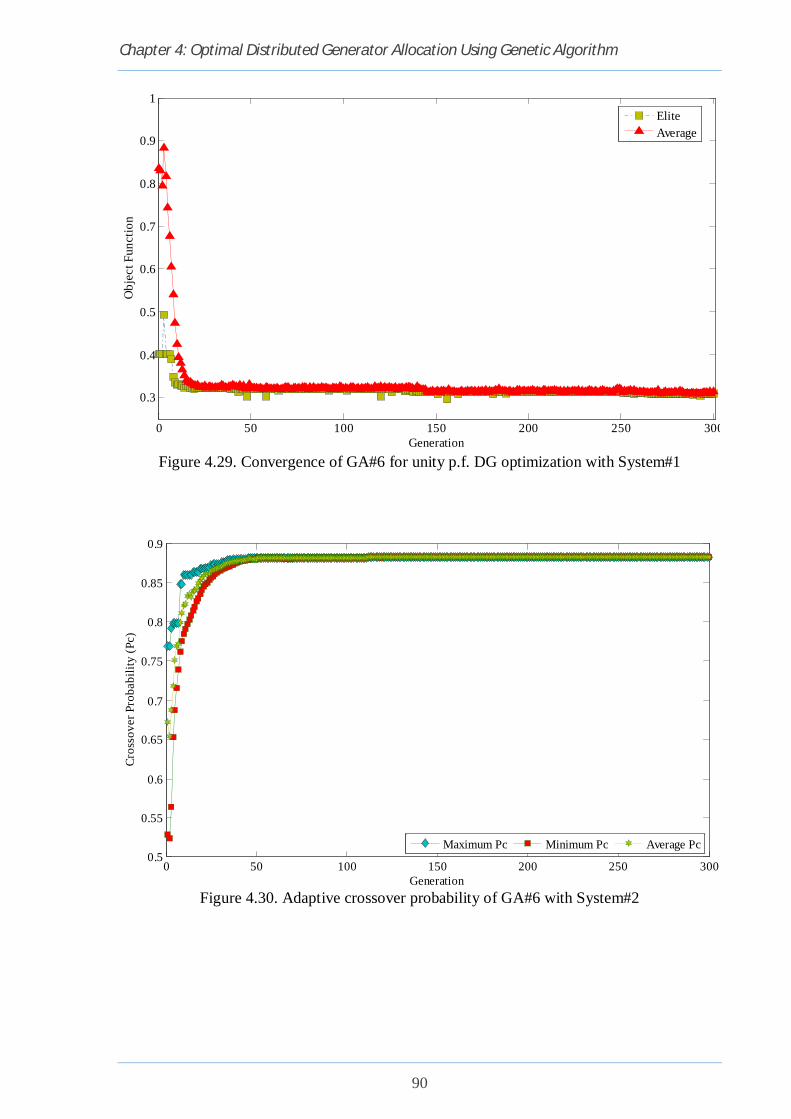
Chapter 4: Optimal Distributed Generator Allocation Using Genetic Algorithm
90
Figure 4.29. Convergence of GA#6 for unity p.f. DG optimization with System#1
0 50 100 150 200 250 300
0.3
0.4
0.5
0.6
0.7
0.8
0.9
1
Generation
Obj
ect F
unct
ion
EliteAverage
Figure 4.30. Adaptive crossover probability of GA#6 with System#2
0 50 100 150 200 250 3000.5
0.55
0.6
0.65
0.7
0.75
0.8
0.85
0.9
Generation
Cros
sove
r Pro
babi
lity
(Pc)
Maximum Pc Minimum Pc Average Pc

Chapter 4: Optimal Distributed Generator Allocation Using Genetic Algorithm
91
Figure 4.31. Variation of adaptive crossover probability of GA#6 in each and every generation with System#2
0.5 20.5 40.5 60.5 80.5 100.5 120.5 140.5 160.5 180.5 200.50.4
0.45
0.5
0.55
0.6
0.65
0.7
0.75
0.8
0.85
0.9Cr
osso
ver P
roba
bilit
y
Generation
Fixed Load & Generation
Figure 4.32. Zooming up the adaptive crossover probability of GA#6 up to generation 50
0 5 10 15 20 25 30 35 40 45 50
0.55
0.6
0.65
0.7
0.75
0.8
0.85
Cro
ssov
er P
roba
bilit
y
Generation
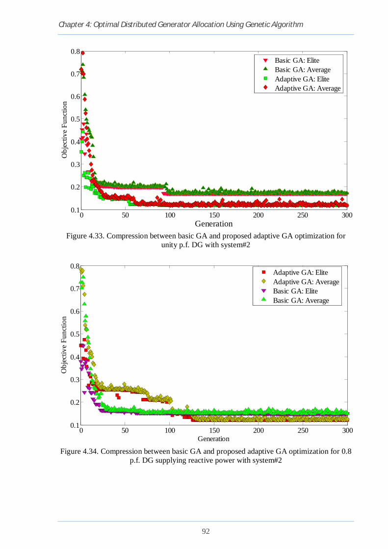
Chapter 4: Optimal Distributed Generator Allocation Using Genetic Algorithm
92
Figure 4.33. Compression between basic GA and proposed adaptive GA optimization for unity p.f. DG with system#2
0 50 100 150 200 250 3000.1
0.2
0.3
0.4
0.5
0.6
0.7
0.8
Generation
Obj
ectiv
e Fu
nctio
n
Basic GA: EliteBasic GA: AverageAdaptive GA: EliteAdaptive GA: Average
Figure 4.34. Compression between basic GA and proposed adaptive GA optimization for 0.8 p.f. DG supplying reactive power with system#2
0 50 100 150 200 250 3000.1
0.2
0.3
0.4
0.5
0.6
0.7
0.8
Generation
Obj
ectiv
e Fu
nctio
n
Adaptive GA: EliteAdaptive GA: AverageBasic GA: EliteBasic GA: Average

Chapter 4: Optimal Distributed Generator Allocation Using Genetic Algorithm
93
After analysing the above results, it can be summarised that effectively the proposed adaptive
GA give better results. The convergence criteria of the proposed adaptive GA is well
acceptable. Figure 4.31 and Figure 4.32 shows that the crossover probability is fully adaptive
in nature (i.e. it is not only generation wise also population wise adaptive in nature). The
proposed AGA is tested on both the systems for the all case considered in the study and
satisfactory results are achieved in all cases. The quick convergence of GA and stuck in a local
minima can be avoided by this adaptive crossover approach.
Table 4.15. Different case study for different system with GA#6 optimization
Different Cases
Different systems
No. of
DG
Total DG Power No.
of Tap
No. of
CB
Total CB
Reactive Power (kW)
Optimal Active Power Loss (kW)
Optimal Reactive Power Loss
(kVAR)
Min. Node
Voltage (Volt)
Max Current (Amp)
Active Power (kW)
Reactive Power
(kVAR)
Base System # 1 - - - - - - 224.995 102.198 0.90919 0.49031 System # 2 - - - - - - 887.181 381.694 0.68442 2.43820
Case # 1 (a)
System # 1 4 2088.0 - - - - 50.557 24.0396 0.96953 0.32060 System # 2 5 2095.0 - - - - 92.600 39.839 0.92560 1.30910
Case # 1 (b)
System # 1 5 1678.4 1258.8 - - - 17.624 13.135 0.98035 0.25856 System # 2 6 1679.2 1259.4 - - - 89.619 38.557 0.93813 1.30910
Case # 1 (c)
System # 1 3 1433.6 -1075.6 - - - 190.731 85.864 0.93621 0.46614 System # 2 4 1650.4 -1237.8 - - - 535.504 230.391 0.82221 2.11770
Case # 2 (a)
System # 1 5 2087.0 - 8 - - 16.598 9.694 0.97902 0.23973 System # 2 6 2095.0 - 19 - - 77.164 33.059 0.93456 1.30910
Case # 2 (b)
System # 1 5 1676.0 1257.0 9 - - 7.698 4.534 0.98803 0.21735 System # 2 6 1678.4 1258.8 20 - - 76.789 33.037 0.95106 1.30830
Case # 2 (c)
System # 1 4 1634.4 -1225.8 10 - - 128.582 56.112 0.95070 0.36631 System # 2 4 1658.4 -1243.8 20 - - 483.191 207.885 0.84036 1.91430
Case # 3 System # 1 - - - - 4 2099 128.676 57.0404 0.93814 0.40236 System # 2 - - - - 4 2096 786.995 338.591 0.71626 2.25760
Case # 4 System # 1 - - - 7 4 2091 120.470 56.114 0.94519 0.39981 System # 2 - - - 20 4 2090 716.607 308.308 0.75746 2.12410
Case # 5 System # 1 - - - 10 - - 169.244 77.768 0.91721 0.43167 System # 2 - - - 20 - - 796.285 342.588 0.73196 2.26360
case#1(a), unity p.f. DG; case#1(b), DG operating at 0.8 p.f. leading; case#1(c), DG operating at 0.8 p.f. lagging; case#2(a), unity p.f. DG with OLCT; case#2(b), DG operating at 0.8 p.f. leading with OLTC.; case#2(c), DG operating at 0.8 p.f. lagging with OLTC; case#3, capacitor bank; case#4, capacitor bank with OLTC; case#5, only OLTC.

Chapter 4: Optimal Distributed Generator Allocation Using Genetic Algorithm
94
4.10 CASE STUDY FOR SELECTION OF UNCROSSED PARENTS
The offspring can be selected by two different method (i) best fitness parent among the parent
pair and (ii) the chromosome belongs the same location or number of the selected parent’s
pair location or number in the population and matting pool respectively. The study is carried
on the system#2 with GA#6 and the results are shown in the Table 4.16 below.
Table 4.16. Comparison of various uncrossed parents selection approach of GA optimization for dg allocation
Case Type of Approach
Minimum Active Power Loss (kW)
Average Active Power Loss
(kW) Minimum Voltage Average Objective
Function
Elite Mean Value
Standard Deviation
Mean Value
Standard Deviation
Minimum Value
Mean Value
Standard Deviation
Mean Value
Standard Deviation
1(a) First 50.913 66.426 9.165 72.702 8.548 0.93370 0.94500 0.00450 0.12190 0.00540
Second 45.649 59.642 9.319 65.573 10.720 0.93040 0.93930 0.00450 0.13690 0.00640
1(b) First 62.980 65.120 1.291 68.091 2.366 0.95000 0.95150 0.00190 0.11910 0.00360
Second 64.601 68.152 2.737 70.879 3.122 0.94130 0.94980 0.00220 0.12330 0.00490
1(c) First 474.75 536.77 22.844 561.35 13.756 0.82425 0.83348 0.00486 0.58249 0.00505
Second 484.04 540.28 21.109 559.18 15.663 0.78370 0.83064 0.01094 0.58352 0.01514
2(a) First 38.139 50.454 8.756 54.828 8.864 0.94301 0.94979 0.00403 0.11443 0.00410
Second 41.652 51.656 7.357 56.233 7.688 0.94124 0.94846 0.00391 0.11709 0.00593
2(b) First 50.191 53.987 1.875 57.001 2.794 0.95362 0.95581 0.00268 0.10053 0.00377
Second 52.423 56.212 2.222 59.661 2.778 0.95300 0.95490 0.00230 0.10980 0.00480
2(c) First 441.61 483.60 16.922 504.74 12.403 0.82323 0.84981 0.00698 0.52509 0.00817
Second 422.68 471.94 24.719 495.53 21.399 0.82810 0.84880 0.00770 0.52120 0.01160
3 First 778.25 778.58 0.1906 779.26 0.5583 0.71840 0.71890 0.00020 0.88520 0.00070
Second 778.31 778.68 0.2119 779.35 0.5547 0.71820 0.71880 0.00020 0.88540 0.00070
4 First 708.69 713.04 2.099 714.54 2.157 0.77970 0.78430 0.00080 0.78630 0.00250
Second 708.10 712.91 2.643 714.51 2.667 0.75630 0.75870 0.00100 0.78640 0.00310
5 First 792.09 797.21 3.284 798.57 3.441 0.72980 0.73100 0.00080 0.87730 0.00320
Second 792.50 796.18 2.046 797.62 2.146 0.73033 0.73130 0.00052 0.87639 0.00202
case#1(a), unity p.f. DG; case#1(b), DG operating at 0.8 p.f. leading; case#1(c), DG operating at 0.8 p.f. lagging; case#2(a), unity p.f. DG with OLCT; case#2(b), DG operating at 0.8 p.f. leading with OLTC.; case#2(c), DG operating at 0.8 p.f. lagging with OLTC; case#3, capacitor bank; case#4, capacitor bank with OLTC; case#5, only OLTC.

Chapter 4: Optimal Distributed Generator Allocation Using Genetic Algorithm
95
After analysing the above results, it can be summarised that the first approach is better than
second (i.e. when the crossover criteria is not satisfied then the offspring will bear only
chromosome belongs the same location or number of the selected parent’s pair location or
number in the population and matting pool respectively). These selection give better voltage
profile and low power losses in almost all cases except the case#5 in which only OLTC is
controlling the voltage and minimizing the power losses.
Chapter 4: Optimal Distributed Generator Allocation Using Genetic Algorithm
96
4.11 SUMMARY
In this chapter, a deterministic method to find the optimal DG sizing and placement in a
distribution network was proposed, where the total real power loss of the network were
employed as the objective to be minimised. Both the single-objective and multi-objective
optimization method was employed for DG allocation issue. After analysing the above results,
it can be summarised that DG placement in the distribution system is profitable. DG not only
minimised the power loss of the distribution system also it improved the voltage profile. The
multi-objective optimization give the better optimal result then the single-objective
optimization. All the adaptive GA gives a well constricted result. But, some of the GA give
more satisfactory results (i.e. less standard dilation, low minimum power loss in the
generations, high minimum node voltage compare to other, etc.). The second objective function
approach gives the better performance with all the adaptive GA and particularly with basic GA
compare to first objective function approach. Though the basic GA have a quick convergence
criteria it can provide considerable optimal results. Results shows that GA#3 have the best
result among all of the GA previously proposed by others though the GA is partially adaptive
in nature. The proposed adaptive GA gives the most satisfactory and acceptable result among
all the GA approach is considered in the study. The proposed GA give the better result in all
part of optimization (i.e. in case for minimum voltage and power loss).
The convergence criteria of the proposed adaptive GA is well acceptable. The crossover
probability of proposed GA is fully adaptive in nature (i.e. it is not only generation wise also
population wise adaptive in nature). The quick convergence of GA and stuck in a local minima
can be avoided by this adaptive crossover approach. Synchronous DG are profitable application
in all type of system also induction DG are considerable profitable though they consumed
reactive power from the system. Installation of induction DG in a very week distribution system
is better than the capacitor placement.

97
CHAPTER-5
OPTIMAL DG ALLOCATION UNDER VARIABLE LOAD
AND GENERATION USING GENETIC ALGORITHM
5.1 INTRODUCTION
Distributed generation (DG) technologies under smart grid concept forms the backbone of our
world Electric distribution networks [5]. These DG technologies are classified into two
categories: (i) renewable energy sources (RES) and (ii) fossil fuel-based sources. Renewable
energy source (RES) based DGs are wind turbines, photovoltaic, biomass, geothermal, small
hydro, etc. Fossil fuel based DGs are the internal combustion engines (IC), combustion
turbines and fuel cells. Environmental, economic and technical factors have a huge role in DG
development [3] [6-7]. In accord with the Kyoto agreement on climate change, many efforts
to reduce carbon emissions have been taken, and as a result of which, the penetration of DGs
in distribution systems rises [8]. Presence of Distributed generation in distribution networks
is a momentous challenge in terms of technical and safety issues [12–14]. Thus, it is critical
to evaluate the technical impacts of DG in power networks. Thus, the generators are needed
to be connected in distributed systems in such a manner that it avoids degradation of power
quality and reliability. Evaluation of the technical impacts of DG in the power networks is
very critical and laborious. Inadequate allocation of DG in terms of its location and capacity
may lead to increase in fault currents, causes voltage variations, interfere in voltage-control
processes, diminish or increase losses, increase system capital and operating costs, etc.[13].
The placement of the DG units mainly the Renewable energy sources placement, is affected
by several factors such as wind speed, solar irradiation, environmental factors, geographical
topography, political factors, etc. For example, wind generators or turbines cannot be installed
near residential areas, because of the interference in the form of public reactions and
legislations from environmental organisations. Another issue is application of the plug-in
electric vehicle (PEV) which is being paid more attention to [44-46]. However, there are
several factors or uncertainties that can possibly lead to probable risks in determining the

Chapter 5: Optimal DG Allocation under Variable Load and Generation
98
optimal siting and sizing of DGs in distribution system planning [47]. Some of the
uncertainties are possibilistic output power of a PEV due to its alteration of
charging/discharging schedule [48-50], wind power unit due to frequent variable wind speed,
from a solar generating source due to the possibilistic illumination intensity, volatile fuel
prices and future uncertain load growth. The most essential uncertainty to account for the
time-varying characteristics of both generation and demand of power are these increasing
penetrations of variable renewable generators with wind power [47][53], being the most
noteworthy of them.
5.2 MULTI-OBJECTIVE PLANNING OF RADIAL DISTRIBUTION
NETWORKS USING PLGM
In most of the planning models, the optimal distribution network is determined based on a
deterministic load demand which is usually obtained from a load forecast and DG generation.
The optimal DG power generation of a distribution network is determined based on the DG
generation (i.e., electric utilities and customers) and weather forecast in the form of wind or
solar power generation. However, such a forecast is always subject to some error. Since the
operating conditions (e.g. node voltage, branch current, illumination of sun, wind speed, etc.)
of any distribution network depend on the load, a network operating with loads that differ from
the nominal ones may be subject to violations of the acceptable operating conditions. In this
study, load demand uncertainty (LDU) and DG power generation uncertainty (PGU) is
incorporated into network planning to investigate its overall influence on planned networks. A
possibilistic (fuzzy-based) approach can be used to model the uncertainty of LDU and PGU.
Possibilistic approach, ambiguity of load demand and DG power generation can be modelled
efficiently without any problem-specific knowledge. A fuzzy membership function can be used
to model this inexplicit and uncertain information, providing degrees of membership to all
possible values of the load demand and DG power generation for each and candidate node
respectively.

Chapter 5: Optimal DG Allocation under Variable Load and Generation
99
5.2.1 Possibilistic Load and Generation Model (PLGM)
A fuzzy number is a special case of a convex, normalized fuzzy set representing an
extension of real numbers. It is used to transform the verbal declaration of an uncertain number
or an interval into its mathematical form. Fuzzy numbers allow the incorporation of uncertainty
on parameters, properties, geometry, initial conditions, etc. A fuzzy number can be
characterized by various mathematical functions [62, 63]. Load demand uncertainty (LDU) and
DG power generation uncertainty (PGU) typically represented by triangular or trapezoidal
fuzzy numbers [64], as shown in Figure 5.1 and Figure 5.3. In practice, the most probable load
for each node of a distribution networks is forecasted by utility companies using it’s high and
low bounds. In this context, a triangular fuzzy number is a more practical way of translating
this fuzzy information into an uncertainty range (an interval) plus an interior “most credible”
value, which is obtained from the forecast [64]. Distributed generation is at present being used
by customers to various purposes (i.e., to meet some or all of their electricity needs, to reduce
demand charges by their electric utility, provide backup power, etc.). Also electric utilities are
using their won controlled DG networks to enhance their distribution networks. Due to some
electric utility controlled DG and customers uncontrolled DG, DG power generation
uncertainty (PGU) typically represented by triangular fuzzy numbers. Thus, in this work, the
load demand at each node and the DG power generation at candidate nodes are considered as
a possibilistic variable represented by two different triangular fuzzy number. For load demand
퐿 = (퐿 _ , 퐿 , 퐿 _ ) as shown in Figure 5.1, in which 퐿 _ , 퐿 and 퐿 _ represent
the minimum possible load demand, load demand with highest possibility of existence, and
maximum possible load demand for a node, and for DG power generation 푃 =
(푃 _ ,푃 ,푃 _ ) as shown in Figure 5.2, in which 푃 _ , 푃 and 푃 _
represent the minimum possible DG power generation, DG power generation with highest
possibility of existence, and maximum possible DG power generation for a candidate node.
The objective functions is a function of load demand and DG power generation, which is also
become possibilistic quantities (i.e., fuzzy numbers).

Chapter 5: Optimal DG Allocation under Variable Load and Generation
100
5.2.2 Comparison of Fuzzy Numbers
Fuzzy numbers forms the objective function for the optimization problem discussed in
the study as a result of which direct comparison between two solutions is difficult. Hence, a
suitable de-fuzzification approach is required of which a lot of literatures are available in [65-
66]. The approach used in this study involves transforming of each index of the fuzzy quantities
into real numbers where there is no need for a reference set or a fuzzy relation. In this case for
de-fuzzification various approaches can be used (i.e., center of gravity (COG), mean of maxima
(MOM), total distance criterion (TDC) index and fuzzy removal techniques) [67].COG ascribes
relatively higher weights to lower membership values whereas MOM neglects lower
membership values. TDC and removal techniques are basically equivalent [67]. The TDC or
removal value is the average of the sum of areas under the left and right sides of the fuzzy
membership function corresponding to an 훼-level. The method used in this study yields a
reasonably good representation of a fuzzy set [53, 54]. In the present study, the removal
Figure 5.1. Possibilistic variable, i.e., possibilistic load demand, as a triangular fuzzy number,
Figure 5.2 Possibilistic variable, i.e., possibilistic DG power
generation, as a triangular fuzzy number,
Figure 5.3. Fuzzy removal technique for a possibilistic objective function.
Figure 5.4. Fuzzy removal technique for a possibilistic objective
function.

Chapter 5: Optimal DG Allocation under Variable Load and Generation
101
technique was used to obtain equivalent crisp values of the fuzzy objective functions. For a
triangular fuzzy number, the removal {푅푒푚 푓 } of a fuzzy objective function 푓
corresponding to an 훼 -cut is defined as (Ramirez-Rosado & Dominiguez-Navarra, 2004)
(Figure 5.5):
푅푒푚 푓 = (푓 + 2 ∗ 푓 + 푓 )/4 (5.1)
Two fuzzy numbers, 푎 and 푏 , can be compared using their corresponding removal values
푅푒푚(푎)and푅푒푚(푏). The value of 훼 is user specific.
5.3 OBJECTIVE FUNCTIONS
A multi-objective optimization problem is consider in this distribution networks
planning problem with continuous planning decision variables. The main objective is to
determine an economical yet reliable network with better technical features, such as lower
power loss, better node voltage profile, and better branch current/thermal limit ratio. Thus, two
objective functions are formulated: minimization of (i) the total power loss (푃 )of the
distribution network and (ii) maximum node voltage deviation(푉 ) ratio. Optimization of (i)
yields an economical and high efficient network and optimization of (ii) results in a reliable
network with better technical features.
푅푒푚(푓 ) = ∑ _
∑ _ ∀푖 = 푁 (5.2)
Figure 5.5. Fuzzy removal technique for a possibilistic objective function.
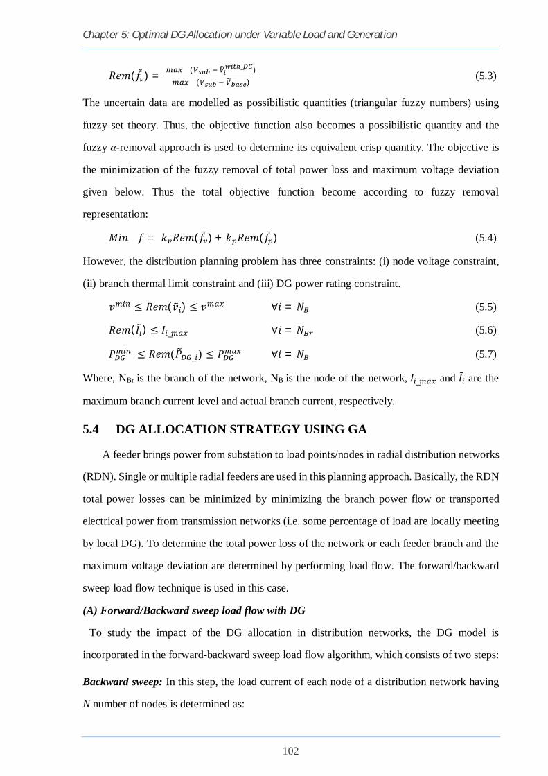
Chapter 5: Optimal DG Allocation under Variable Load and Generation
102
푅푒푚(푓 ) = ( _ )( )
(5.3)
The uncertain data are modelled as possibilistic quantities (triangular fuzzy numbers) using
fuzzy set theory. Thus, the objective function also becomes a possibilistic quantity and the
fuzzy α-removal approach is used to determine its equivalent crisp quantity. The objective is
the minimization of the fuzzy removal of total power loss and maximum voltage deviation
given below. Thus the total objective function become according to fuzzy removal
representation:
푀푖푛푓 = 푘 푅푒푚(푓 ) + 푘 푅푒푚(푓 ) (5.4)
However, the distribution planning problem has three constraints: (i) node voltage constraint,
(ii) branch thermal limit constraint and (iii) DG power rating constraint.
푣 ≤ 푅푒푚(푣 ) ≤ 푣 ∀푖 = 푁 (5.5)
푅푒푚(퐼 ) ≤ 퐼 _ ∀푖 = 푁 (5.6)
푃 ≤ 푅푒푚(푃 _ ) ≤ 푃 ∀푖 = 푁 (5.7)
Where, NBr is the branch of the network, NB is the node of the network, 퐼 _ and 퐼 are the
maximum branch current level and actual branch current, respectively.
5.4 DG ALLOCATION STRATEGY USING GA
A feeder brings power from substation to load points/nodes in radial distribution networks
(RDN). Single or multiple radial feeders are used in this planning approach. Basically, the RDN
total power losses can be minimized by minimizing the branch power flow or transported
electrical power from transmission networks (i.e. some percentage of load are locally meeting
by local DG). To determine the total power loss of the network or each feeder branch and the
maximum voltage deviation are determined by performing load flow. The forward/backward
sweep load flow technique is used in this case.
(A) Forward/Backward sweep load flow with DG
To study the impact of the DG allocation in distribution networks, the DG model is
incorporated in the forward-backward sweep load flow algorithm, which consists of two steps:
Backward sweep: In this step, the load current of each node of a distribution network having
N number of nodes is determined as:

Chapter 5: Optimal DG Allocation under Variable Load and Generation
103
퐼 ̅ (푚) = ( ) ( )∗( )
[푚 = 1,2,3 … … …푁] (5.8)
where, 푃 (푚) and 푄 (푚) represent the active and reactive power demand at node m and the
overbar notation (푥̅) indicates the phasor quantities, such as 퐼 ̅ ,푉∗.Then, the current in each
branch of the network is computed as:
퐼(̅푚푛) = 퐼 ̅ (푛) + ∑ 퐼 ̅ (푚)∈ (5.9)
where, the setΓ consists of all nodes which are located beyond the node n. To incorporate the
DG model, the active and reactive power demand at the node at which a DG unit is placed, say,
at node i, is modified by:
푃 __ = 푃 _
_ − 푃 _ (5.10)
푄 __ = 푄 _
_ ∓푄 _ (5.11)
Forward sweep: This step is used after the backward sweep so as to determine the voltage at
each node of a distribution network as follows:
푉(푛) = 푉(푚)− 퐼(̅푚푛)푍(푚푛) (5.12)
where, nodes n and m represent the receiving and sending end nodes, respectively for the branch
mn and 푍(푚푛) is the impedance of the branch.
(B) GA Optimization for DG allocation
In this analysis proposed adaptive GA is used for optimization of DG location and size.
Optimization procedure is same as discussed in section 4.4 and section 4.5. Only the load flow
is fuzzyfied and the GA is in adaptive in nature. The flowchart for the uncertainty in load and
generation approach is presented below.
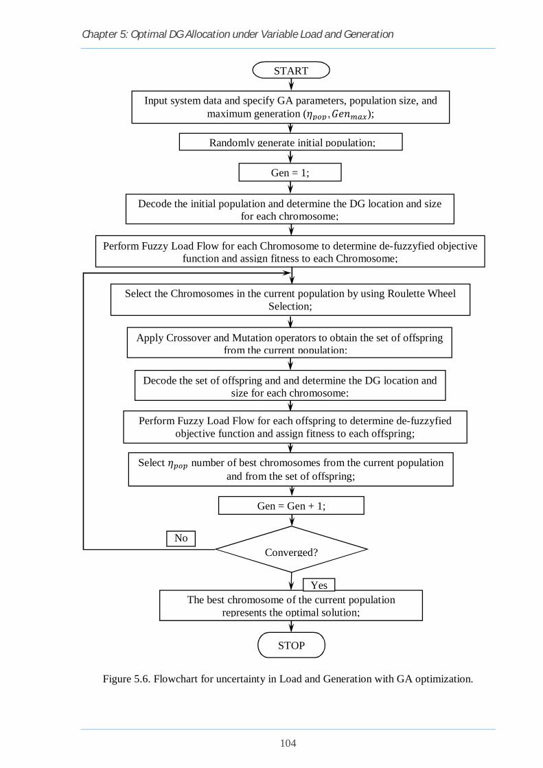
Chapter 5: Optimal DG Allocation under Variable Load and Generation
104
Figure 5.6. Flowchart for uncertainty in Load and Generation with GA optimization.
START
Input system data and specify GA parameters, population size, and maximum generation (휂 ,퐺푒푛 );
Randomly generate initial population;
Gen = 1;
Decode the initial population and determine the DG location and size for each chromosome;
Perform Fuzzy Load Flow for each Chromosome to determine de-fuzzyfied objective function and assign fitness to each Chromosome;
Select the Chromosomes in the current population by using Roulette Wheel Selection;
Apply Crossover and Mutation operators to obtain the set of offspring from the current population;
Perform Fuzzy Load Flow for each offspring to determine de-fuzzyfied objective function and assign fitness to each offspring;
Decode the set of offspring and and determine the DG location and size for each chromosome;
Select 휂 number of best chromosomes from the current population and from the set of offspring;
Gen = Gen + 1;
Converged?
The best chromosome of the current population represents the optimal solution;
STOP
Yes
No

Chapter 5: Optimal DG Allocation under Variable Load and Generation
105
5.5 CASE STUDY FOR UNCERTAINTY IN LOAD AND GENERATION
5.5.1 Deterministic load and generation analysis
Table 5.1 Study for deterministic load of 0.6 p.u. on test systems with Ga#6 optimization
Different Cases
Different systems
No. of
DG
Total DG Power No.
of Tap
No. of
CB
Total CB Reactive Power (kW)
Minimum Active Power Loss (kW)
Minimum Reactive Power Loss
(kVAR)
Min. Node
Voltage (Volt)
Max Current (Amp)
Active Power (kW)
Reactive Power
(kVAR)
Base System # 1 - - - - - - 75.5264 34.4477 0.94755 0.28777 System # 2 - - - - - - 241.251 103.794 0.84120 1.24020
Case # 1 (a)
System # 1 5 1398.0 - - - - 17.115 7.994 0.98560 0.18710 System # 2 4 1394.0 - - - - 22.128 9.520 0.96155 0.85695
Case # 1 (b)
System # 1 4 1118.4 838.8 - - - 4.032 3.636 0.99234 0.14046 System # 2 5 1115.2 836.4 - - - 24.488 10.535 0.97053 0.87447
Case # 1 (c)
System # 1 3 1019.2 -764.4 - - - 66.918 29.960 0.96530 0.27684 System # 2 3 1093.6 -820.2 - - - 125.231 53.878 0.88240 1.36410
Case # 2 (a)
System # 1 4 1397.0 - 10 - - 4.814 2.742 0.99419 0.14526 System # 2 4 1394.0 - 19 - - 11.874 5.108 0.96789 0.76714
Case # 2 (b)
System # 1 4 1118.4 838.8 10 - - 0.164 2.028 0.99487 0.12917 System # 2 5 1145.2 836.2 20 - - 14.859 6.393 0.97164 0.78049
Case # 2 (c)
System # 1 3 1115.2 -836.4 9 - - 36.222 16.880 0.97204 0.23973 System # 2 3 1115.2 -834.4 20 - - 104.621 45.011 0.89680 1.30790
Case # 3 System # 1 - - - - 4 1396 41.750 18.292 0.96443 0.23564 System # 2 - - - - 3 1394 218.801 94.135 0.85533 1.16640
Case # 4 System # 1 - - - 10 4 1398 37.337 16.783 0.96768 0.23472 System # 2 - - - 20 3 1390 200.815 86.397 0.87695 1.10720
Case # 5 System # 1 - - - 10 - - 49.156 22.526 0.95545 0.23938 System # 2 - - - 20 - - 218.739 94.108 0.86491 1.15550
System # 1 and System # 2 with a deterministic load of 0.6 p.u base Load; case#1(a), unity p.f. DG; case#1(b), DG operating at 0.8 p.f. leading; case#1(c), DG operating at 0.8 p.f. lagging; case#2(a), unity p.f. DG with OLCT; case#2(b), DG operating at 0.8 p.f. leading with OLTC.; case#2(c), DG operatingat 0.8 p.f. lagging with OLTC; case#3, capacitor bank; case#4, capacitor bank with OLTC; case#5, only OLTC.

Chapter 5: Optimal DG Allocation under Variable Load and Generation
106
Table 5.2. Study for deterministic load of 1.0 p.u. on test systems with Ga#6 optimization
Different Cases
Different systems
No. of
DG
Total DG Power No.
of Tap
No. of
CB
Total CB Reactive Power (kW)
Minimum Active Power Loss (kW)
Minimum Reactive Power Loss
(kVAR)
Min. Node
Voltage (Volt)
Max Current (Amp)
Active Power (kW)
Reactive Power
(kVAR)
Base System # 1 - - - - - - 224.995 102.198 0.90919 0.49031 System # 2 - - - - - - 887.181 381.694 0.68442 2.43820
Case # 1 (a)
System # 1 4 2088.0 - - - - 50.557 24.0396 0.96953 0.32060 System # 2 5 2095.0 - - - - 92.600 39.839 0.92560 1.30910
Case # 1 (b)
System # 1 5 1678.4 1258.8 - - - 17.624 13.135 0.98035 0.25856 System # 2 6 1679.2 1259.4 - - - 89.619 38.557 0.93813 1.30910
Case # 1 (c)
System # 1 3 1433.6 -1075.6 - - - 190.731 85.864 0.93621 0.46614 System # 2 4 1650.4 -1237.8 - - - 535.504 230.391 0.82221 2.11770
Case # 2 (a)
System # 1 5 2087.0 - 8 - - 16.598 9.694 0.97902 0.23973 System # 2 6 2095.0 - 19 - - 77.164 33.059 0.93456 1.30910
Case # 2 (b)
System # 1 5 1676.0 1257.0 9 - - 7.698 4.534 0.98803 0.21735 System # 2 6 1678.4 1258.8 20 - - 76.789 33.037 0.95106 1.30830
Case # 2 (c)
System # 1 4 1634.4 -1225.8 10 - - 128.582 56.112 0.95070 0.36631 System # 2 4 1658.4 -1243.8 20 - - 483.191 207.885 0.84036 1.9143
Case # 3 System # 1 - - - - 4 2099 128.676 57.0404 0.93814 0.40236 System # 2 - - - - 4 2096 786.995 338.591 0.71626 2.25760
Case # 4 System # 1 - - - 7 4 2091 120.470 56.114 0.94519 0.39981 System # 2 - - - 20 4 2090 716.607 308.308 0.75746 2.12410
Case # 5 System # 1 - - - 10 - - 169.244 77.768 0.91721 0.43167 System # 2 - - - 20 - - 796.285 342.588 0.73196 2.26360
System # 1 and System # 2 with a deterministic load of 1.0 p.u Load; case#1(a), unity p.f. DG; case#1(b), DG operating at 0.8 p.f. leading; case#1(c), DG operating at 0.8 p.f. lagging; case#2(a), unity p.f. DG with OLCT; case#2(b), DG operating at 0.8 p.f. leading with OLTC.; case#2(c), DG operating at 0.8 p.f. lagging with OLTC; case#3, capacitor bank; case#4, capacitor bank with OLTC; case#5, only OLTC.
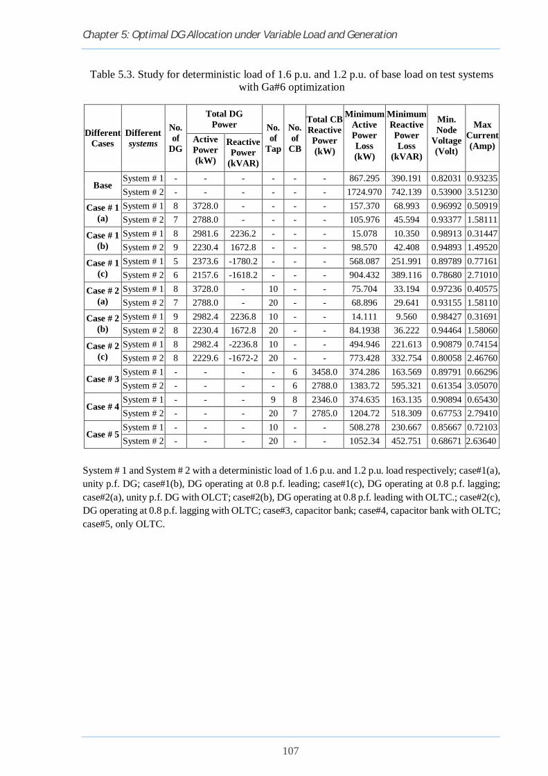
Chapter 5: Optimal DG Allocation under Variable Load and Generation
107
Table 5.3. Study for deterministic load of 1.6 p.u. and 1.2 p.u. of base load on test systems with Ga#6 optimization
Different Cases
Different systems
No. of
DG
Total DG Power No.
of Tap
No. of
CB
Total CB Reactive Power (kW)
Minimum Active Power Loss (kW)
Minimum Reactive Power Loss
(kVAR)
Min. Node
Voltage (Volt)
Max Current (Amp)
Active Power (kW)
Reactive Power
(kVAR)
Base System # 1 - - - - - - 867.295 390.191 0.82031 0.93235 System # 2 - - - - - - 1724.970 742.139 0.53900 3.51230
Case # 1 (a)
System # 1 8 3728.0 - - - - 157.370 68.993 0.96992 0.50919 System # 2 7 2788.0 - - - - 105.976 45.594 0.93377 1.58111
Case # 1 (b)
System # 1 8 2981.6 2236.2 - - - 15.078 10.350 0.98913 0.31447 System # 2 9 2230.4 1672.8 - - - 98.570 42.408 0.94893 1.49520
Case # 1 (c)
System # 1 5 2373.6 -1780.2 - - - 568.087 251.991 0.89789 0.77161 System # 2 6 2157.6 -1618.2 - - - 904.432 389.116 0.78680 2.71010
Case # 2 (a)
System # 1 8 3728.0 - 10 - - 75.704 33.194 0.97236 0.40575 System # 2 7 2788.0 - 20 - - 68.896 29.641 0.93155 1.58110
Case # 2 (b)
System # 1 9 2982.4 2236.8 10 - - 14.111 9.560 0.98427 0.31691 System # 2 8 2230.4 1672.8 20 - - 84.1938 36.222 0.94464 1.58060
Case # 2 (c)
System # 1 8 2982.4 -2236.8 10 - - 494.946 221.613 0.90879 0.74154 System # 2 8 2229.6 -1672-2 20 - - 773.428 332.754 0.80058 2.46760
Case # 3 System # 1 - - - - 6 3458.0 374.286 163.569 0.89791 0.66296 System # 2 - - - - 6 2788.0 1383.72 595.321 0.61354 3.05070
Case # 4 System # 1 - - - 9 8 2346.0 374.635 163.135 0.90894 0.65430 System # 2 - - - 20 7 2785.0 1204.72 518.309 0.67753 2.79410
Case # 5 System # 1 - - - 10 - - 508.278 230.667 0.85667 0.72103 System # 2 - - - 20 - - 1052.34 452.751 0.68671 2.63640
System # 1 and System # 2 with a deterministic load of 1.6 p.u. and 1.2 p.u. load respectively; case#1(a), unity p.f. DG; case#1(b), DG operating at 0.8 p.f. leading; case#1(c), DG operating at 0.8 p.f. lagging; case#2(a), unity p.f. DG with OLCT; case#2(b), DG operating at 0.8 p.f. leading with OLTC.; case#2(c), DG operating at 0.8 p.f. lagging with OLTC; case#3, capacitor bank; case#4, capacitor bank with OLTC; case#5, only OLTC.

Chapter 5: Optimal DG Allocation under Variable Load and Generation
108
5.5.2 Possibilistic load and generation analysis
Table 5.4. Study for possibilistic load of 0.4 p.u to 1.4 p.u. on test systems with Ga#6 optimization
Different Cases
Different systems
No. of
DG
Total DG Power No.
of Tap
No. of
CB
Total CB Reactive Power (kW)
Minimum Active Power Loss (kW)
Minimum Reactive Power Loss
(kVAR)
Min. Node
Voltage (Volt)
Max Current (Amp)
Active Power (kW)
Reactive Power
(kVAR)
Base System # 1 - - - - - - 201.193 91.435 0.91416 0.46444 System # 2 - - - - - - 764.177 328.774 0.70890 2.25270
Case # 1 (a)
System # 1 7 2213.0 - - - - 49.174 21.871 0.98114 0.29830 System # 2 7 2207.0 - - - - 59.896 25.769 0.94218 1.24160
Case # 1 (b)
System # 1 6 1770.4 1327.8 - - - 10.003 9.095 0.98860 0.22293 System # 2 9 1765.6 1324.2 - - - 58.806 25.300 0.95715 1.18690
Case # 1 (c)
System # 1 4 1529.6 -1147.2 - - - 176.867 78.843 0.94305 0.44430 System # 2 6 1759.2 -1319.4 - - - 480.434 206.698 0.83001 1.88320
Case # 2 (a)
System # 1 6 2213.0 - 10 - - 12.781 6.527 0.98875 0.19997 System # 2 6 2206.0 - 18 - - 39.247 16.885 0.94462 1.24160
Case # 2 (b)
System # 1 5 1766.4 1324.8 10 - - 4.004 2.892 0.99454 0.18590 System # 2 8 1765.6 1324.2 19 - - 47.984 20.644 0.95665 1.24280
Case # 2 (c)
System # 1 5 1700.0 -1275.0 10 - - 133.115 59.834 0.95312 0.40433 System # 2 5 1763.2 -1322.4 20 - - 436.000 187.581 0.86231 1.87720
Case # 3 System # 1 - - - - 5 2213.0 116.100 50.726 0.94395 0.37919 System # 2 - - - - 4 2207.0 675.519 290.630 0.73967 2.08190
Case # 4 System # 1 - - - 8 5 2212.0 108.008 47.871 0.94566 0.37645 System # 2 - - - 20 5 2203.0 621.814 267.525 0.77587 1.97270
Case # 5 System # 1 - - - 10 - - 148.999 68.500 0.92255 0.40624 System # 2 - - - 20 - - 691.949 297.699 0.75144 2.10830
System # 1 and System # 2 with a possibilistic load of 0.4 p.u to 1.4 p.u. base Load; case#1(a), unity p.f. DG; case#1(b), DG operating at 0.8 p.f. leading; case#1(c), DG operating at 0.8 p.f. lagging; case#2(a), unity p.f. DG with OLCT; case#2(b), DG operating at 0.8 p.f. leading with OLTC.; case#2(c), DG operating at 0.8 p.f. lagging with OLTC; case#3, capacitor bank; case#4, capacitor bank with OLTC; case#5, only OLTC.

Chapter 5: Optimal DG Allocation under Variable Load and Generation
109
5.5.3 Multiple run for deterministic and possibilistic load and generation
Figure 5.7. System #1, DG location repetition probability for multiple run for the case#1(b); case#1(b), DG operating at 0.8 p.f. leading;
Figure 5.8. System #1, DG location repetition probability for multiple run for the case#1(c); case#1(c), DG operating at 0.8 p.f. lagging;
17 18 21 24 58 59 60 61 62 63 64 650
10
20
30
40
50
60
70
80
90
100
Node Number
Repe
titio
n Pr
obab
ility
Deterministic L & G Possibilistic L Possibilistic G Possibilistic L & G
55 56 57 58 59 60 64 650
10
20
30
40
50
60
70
80
90
100
Node Number
Repe
titio
n Pr
obab
ility
Deterministic L & G Possibilistic L Possibilistic G Possibilistic L & G
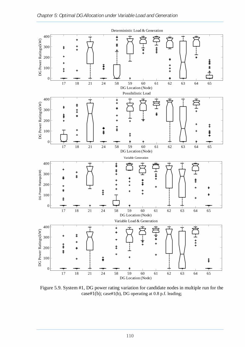
Chapter 5: Optimal DG Allocation under Variable Load and Generation
110
Figure 5.9. System #1, DG power rating variation for candidate nodes in multiple run for the case#1(b); case#1(b), DG operating at 0.8 p.f. leading;
17 18 21 24 58 59 60 61 62 63 64 650
100
200
300
400D
G P
ower
Rat
ings
(kW
)
DG Location (Node)
Deterministic Load & Generation
17 18 21 24 58 59 60 61 62 63 64 650
100
200
300
400
DG
Pow
er R
atin
gs(k
W)
DG Location (Node)
Possibilistic Load
17 18 21 24 58 59 60 61 62 63 64 650
100
200
300
400
DG
Pow
er R
atin
gs(k
W)
DG Location (Node)
Variable Generation
17 18 21 24 58 59 60 61 62 63 64 650
100
200
300
400
DG
Pow
er R
atin
gs(k
W)
DG Location (Node)
Variable Load & Generation

Chapter 5: Optimal DG Allocation under Variable Load and Generation
111
Figure 5.10. System #1, DG power rating variation for candidate nodes in multiple run for the case#1(c); case#1(c), DG operating at 0.8 p.f. lagging;
55 56 57 58 59 60 64 650
100
200
300
400D
G P
ower
Rat
ings
(kW
)
DG Location (Node)
Deterministic Load & Generation
55 56 57 58 59 60 64 650
100
200
300
400
DG
Pow
er R
atin
gs(k
W)
DG Location (Node)
Possibilistic Load
55 56 57 58 59 60 64 650
100
200
300
400
DG
Pow
er R
atin
gs(k
W)
DG Location (Node)
Possibilistic Generation
55 56 57 58 59 60 64 650
100
200
300
400
DG
Pow
er R
atin
gs(k
W)
DG Location (Node)
Possibilistic Load & Generation

Chapter 5: Optimal DG Allocation under Variable Load and Generation
112
Figure 5.11. System #2, DG location repetition probability for multiple run for the case#1(b);
case#1(b), DG operating at 0.8 p.f. leading
Figure 5.12. System #2, DG power rating variation for candidate nodes in multiple run for the
case#1(c); case#1(c), DG operating at 0.8 p.f. lagging
11 12 15 16 18 19 24 36 37 41 44 45 47 49 510
10
20
30
40
50
60
70
80
Node Number
Rep
etiti
on P
roba
bilit
y
Deterministic L & G Possibilistic L Possibilistic G Possibilistic L & G
9 10 16 32 33 35 39 41 45 47 490
10
20
30
40
50
60
70
80
90
100
Node Number
Repe
titio
n Pr
obab
ility
Deterministic L & G Possibilistic L Possibilistic G Possibilistic L & G

Chapter 5: Optimal DG Allocation under Variable Load and Generation
113
Figure 5.13. System #2, DG power rating variation for candidate nodes in multiple run for the case#1(b); case#1(b), DG operating at 0.8 p.f. leading;
11 12 15 16 18 19 24 36 37 41 44 45 47 49 510
100
200
300
400
500
600D
G P
ower
Rat
ings
(kW
)
DG Location (Node)
Deterministic Load & Generation
11 12 15 16 18 19 24 36 37 41 44 45 47 49 510
100
200
300
400
500
600
DG
Pow
er R
atin
gs(k
W)
DG Location (Node)
Possibilistic Load
11 12 15 16 18 19 24 36 37 41 44 45 47 49 510
100
200
300
400
500
600
DG
Pow
er R
atin
gs(k
W)
DG Location (Node)
Possibilistic Generation
11 12 15 16 18 19 24 36 37 41 44 45 47 49 510
100
200
300
400
500
600
DG
Pow
er R
atin
gs(k
W)
DG Location (Node)
Possibilistic Load & Generation

Chapter 5: Optimal DG Allocation under Variable Load and Generation
114
Figure 5.14. System #2, DG power rating variation for candidate nodes in multiple run for the case#1(c);.; case#1(c), DG operating at 0.8 p.f. lagging;
9 10 16 32 33 35 39 41 45 47 490
100
200
300
400
500
600D
G P
ower
Rat
ings
(kW
)
DG Location (Node)
Deterministic Load & Generation
9 10 16 32 33 35 39 41 45 47 490
100
200
300
400
500
600
DG
Pow
er R
atin
gs(k
W)
DG Location (Node)
Possibilistic Load
9 10 16 32 33 35 39 41 45 47 490
100
200
300
400
500
600
DG
Pow
er R
atin
gs(k
W)
DG Location (Node)
Possibilistic Generation
9 10 16 32 33 35 39 41 45 47 490
100
200
300
400
500
600
DG
Pow
er R
atin
gs(k
W)
DG Location (Node)
Possibilistic Load & Generation

Chapter 5: Optimal DG Allocation under Variable Load and Generation
115
5.5.4 Multiple run uncertainty analysis with different system and GA
parameter
With a new system and GA parameter the optimization is carried out for three different cases
(i.e. case#1(a), case#1(b), and case #1(c)). This system and GA parameter are also taken for
the analysis of uncertainty with different DG rating.
Table 5.5. Effective nodes DG ratings median value for various cases
System #1 (69 node) System #2 (52 node) Case#1(b) Case#1(b)
Node no. #AA #BB #CC #DD Node
no. #AA #BB #CC #DD
21 293.5 262.5 325.5 300.5 18 282.5 217 288 233 59 351 337 382 324 36 303 218 260 258.5 60 373.5 365 356 366 44 140 107.5 170.5 108 61 377.5 363 385 371 45 284.5 141 336 129.5 62 362 373 343 328 49 454 452 460 389 63 155.5 124 277.5 139.5 64 368.5 369 376 374
Case#1(c) Case#1(c) 57 397.5 395 397.5 395 16 149.5 0 0 0 58 398 398 398 398 33 557.5 425.5 480.5 322.5 59 397 397 397 397 39 369.5 401 351.5 392 60 357.5 384.5 357.5 384.5 41 100 37 317.5 241 64 364 361 364 361 47 115.5 159.5 0 0
Case#1(b), DG operating at 0.8 p.f. leading; case#1(c), DG operating at 0.8 p.f. lagging and #AA; Deterministic Load and Generation; #BB; Possibilistic Load; #CC; PossibilisticGeneration; #DD; Possibilistic Load and Generation
Table 5.6. GA and network parameters considered for the optimization process
GA parameter Network parameter Population size (Ƞmax) 80 DGs power rating range (PDG): (50 – 600) kW Maximum Generation
(Genmax) 270 Minimum Voltage (Vmin): System#2: 0.90 p.u.
Crossover probability (Ωc) adaptive Maximum Thermal Limit (Imax):
System#2: 1.2 p.u.
Mutation Probability (Ωm) 0.005 Maximum number of DG (ψn): 5 Maximum iteration for load
flow 300 DG penetration limit Max 50% of total load
Accuracy label in load flow 10-9

Chapter 5: Optimal DG Allocation under Variable Load and Generation
116
Table 5.7. Effective nodes DG ratings median value for various cases
System #2 (DG range 50-600) Case#1(a)
Node no. #AA #BB #CC #DD 11 0 0 147.5 0 16 0 483.5 249 0 18 329.5 0 117.5 198 36 0 0 0 0 45 519 502.5 445.5 528.5 47 501.5 466.5 508.5 453.5 49 540.5 543 554.5 518.5
Power Loss 133.03 110.56 103.15 182.39 Minimum Voltage 0.85937 0.88407 0.89363 0.83514
Case#1(b) 11 217 439.5 225 446 16 463 0 466.5 0 18 0 278.5 0 114.5 36 311.5 0 184.5 208 41 0 510 471.5 529 49 527 552 557.5 552
Power Loss 194.04 132.47 113.38 122.78 Minimum Voltage 0.86286 0.90697 0.92554 0.90436
Case#1(c) 33 506.5 347.5 263.5 550.5 39 139 512.5 50.5 488.5 41 439.5 78.5 546 114.5 47 0 298.5 0 0
Power Loss 592.16 563.34 626.14 584.27 Minimum Voltage 0.78064 0.78370 0.76967 0.77897
Case#1(b), DG operating at 0.8 p.f. leading; case#1(c), DG operating at 0.8 p.f. lagging and #AA; Deterministic Load and Generation; #BB; Possibilistic Load; #CC; PossibilisticGeneration; #DD; Possibilistic Load and Generation

Chapter 5: Optimal DG Allocation under Variable Load and Generation
117
5.5.5 Multiple run uncertainty analysis with different DG rating limit
Figure 5.15. Percentage of repetition as DG location in multiple runs for System #2 with a DG rating limit of (50-600) kW
Figure 5.16. Percentage of repetition as DG location in multiple runs for System #2 with a DG rating limit of (50-600) kW Case#1(b), DG operating at 0.8 p.f. leading; and Case# A, Deterministic Load and Generation; Case# B, Possibilistic Load; Case# C, Possibilistic Generation; Case# D, Possibilistic Load and Generation
11 12 16 18 35 36 37 41 43 45 47 490
10
20
30
40
50
60
70
80
90
100
Node Number
Perc
enta
ge o
f Rep
etiti
on a
s D
G L
ocat
ion
in M
ultip
le R
uns
Case#A Case#B Case#C Case#D
11 12 16 18 36 41 43 45 49 510
20
40
60
80
100
110
Node Number
Perc
enta
ge o
f Rep
etiti
on a
s DG
Loc
atio
n in
Mul
tiple
Run
s
Case#A Case#B Case#C Case#D

Chapter 5: Optimal DG Allocation under Variable Load and Generation
118
In uncertainty analysis with different DG rating limit it is concluded that the location of DG is
changes with the DG ratings.
Figure 5.17. Percentage of repetition as DG location in multiple runs for System #2 with a DG rating limit of (50-200) kW
Case#1(b), DG operating at 0.8 p.f. leading; and Case# A, Deterministic Load and Generation; Case# B, Possibilistic Load; Case# C, Possibilistic Generation; Case# D, Possibilistic Load and Generation
13 15 18 19 44 49 50 510
20
40
60
80
100
110
Node Number
Perc
enta
ge o
f Rep
etiti
on a
s DG
Loc
atio
n in
Mul
tiple
Run
s
Case#A Case#B Case#C Case#D
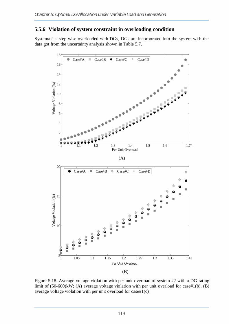
Chapter 5: Optimal DG Allocation under Variable Load and Generation
119
5.5.6 Violation of system constraint in overloading condition
System#2 is step wise overloaded with DGs, DGs are incorporated into the system with the data got from the uncertainty analysis shown in Table 5.7.
(A)
(B)
Figure 5.18. Average voltage violation with per unit overload of system #2 with a DG rating limit of (50-600)kW; (A) average voltage violation with per unit overload for case#1(b), (B) average voltage violation with per unit overload for case#1(c)
1 1.1 1.2 1.3 1.4 1.5 1.6 1.740
2
4
6
8
10
12
14
16
18
Per Unit Overload
Vol
tage
Vio
latio
n (%
)
Case#A Case#B Case#C Case#D
1 1.05 1.1 1.15 1.2 1.25 1.3 1.35 1.415
10
15
20
Per Unit Overload
Vol
tage
Vio
latio
n (%
)
Case#A Case#B Case#C Case#D

Chapter 5: Optimal DG Allocation under Variable Load and Generation
120
(A)
(B)
Figure 5.19. Maximum voltage violation with per unit overload of system #2 with a DG rating limit of (50-600) kW
(A) Maximum voltage violation with per unit overload for case#1(b), (B) maximum voltageviolation with per unit overload for case#1(c)
1 1.1 1.2 1.3 1.4 1.5 1.6 1.740
5
10
15
20
25
30
35
40
45
Per Unit Overload
Vol
tage
Vio
latio
n (%
)
Case#A Case#B Case#C Case#D
1 1.05 1.1 1.15 1.2 1.25 1.3 1.35 1.4110
15
20
25
30
35
40
45
Per Unit Overload
Vol
tage
Vio
latio
n (%
)
Case#A Case#B Case#C Case#D

Chapter 5: Optimal DG Allocation under Variable Load and Generation
121
(A)
(B)
Figure 5.20. Average current violation with per unit overload of system #2 with a DG rating limit of (50-600)
(A) Average current violation with per unit overload for case#1(b), (B) average current violation with per unit overload for case#1(c)
1 1.1 1.2 1.3 1.4 1.5 1.6 1.740
5
10
15
20
25
30
35
40
45
Per Unit Overload
Ther
mal
Lim
it V
iola
tion
(%)
Case#A Case#B Case#C Case#D
1 1.05 1.1 1.15 1.2 1.25 1.3 1.35 1.410
5
10
15
20
25
30
35
40
Per Unit Overload
Ther
mal
Lim
it V
iola
tion
(%)
Case#A Case#B Case#C Case#D

Chapter 5: Optimal DG Allocation under Variable Load and Generation
122
(A)
(B)
Figure 5.19. Maximum current violation with per unit overload of system #2 with a DG rating limit of (50-600)
(A) Maximum current violation with per unit overload for case#1(b), (B) maximum current violation with per unit overload for case#1(c)
1 1.1 1.2 1.3 1.4 1.5 1.6 1.740
10
20
30
40
50
60
70
80
90
100
Per Unit Overload
Ther
mal
Lim
it V
iola
tion
(%)
Case#A Case#B Case#C Case#D
1 1.05 1.1 1.15 1.2 1.25 1.3 1.35 1.410
10
20
30
40
50
60
Per Unit Overload
Ther
mal
Lim
it V
iola
tion
(%)
Case#A Case#B Case#C Case#D

Chapter 5: Optimal DG Allocation under Variable Load and Generation
123
5.6 SUMMARY
In this chapter, a multi-objective optimization method to find the optimal DG sizing and
placement in a distribution network was proposed, where the total real power loss of the
network were employed as the objective to be minimised. Thus, the load demand at each node
and the DG power generation at candidate nodes are considered as a possibilistic variable
represented by two different triangular fuzzy number. An IEEE 69-node radial test distribution
system and 52-node practical radial systems are used to demonstrate the effectiveness of the
proposed methods. The simulation results shows that reduction of power loss in distribution
system is possible and all node voltages variation can be achieved within the required limit if
DG are optimally placed in the system. Induction DG placement into the distribution system
also give a better performance from capacitor bank placement. In modern load growth
scenario uncertainty load and generation model shows that reduction of power loss in
distribution system is possible and all node voltages variation can be achieved within the
required limit without violating the thermal limit of the system.

124
CHAPTER-6
CONCLUSION AND SCOPE FOR FUTURE WORK
6.1 CONCLUSIONS
The installation of DG units in power distribution networks is becoming more
prominent. Consequently, utility companies have started to change their electric infrastructure
to adapt to DGs due to the benefits of DG installation on their distribution systems. These
benefits include reducing power losses, improving voltage profiles, reducing emission impacts
and improving power quality. Additional benefits are avoiding upgrading the present power
systems and preventing a reduction of T&D network capacity during the planning phase.
Nevertheless, achieving these benefits depends highly on the capacity of the DG units and
their installation placement in the distribution systems.
In this work, an innovative approach for management of DG power is represented. The
proposed method deals with optimal selection of nodes for the placement and size of the DG
by using GA. The load flow problem has been solved by forward/backward load flow
methodology. The rating and location has been optimised using Genetic Algorithm. In GA,
coding is developed to carry out the allocation problem, which is identification of location
and rating by one dimensional array. The effectiveness of the approach is demonstrated on
the IEEE 69-node reliability test system and a practical 52-node system.
If DGs are connected to the system, the simulation results concludes that reduction of
active power loss in distribution system is possible and all node voltages variation can be
achieved within the required limit. Multi-objective optimization give the better optimal result
then the single-objective optimization. Induction DGs are connected into the systems power
loss and voltage profile is better from when the capacitor bank is connected into the systems,
though the induction DGs are consuming reactive power from the system where extra amount
of power loss is occur due to reactive power flow through the line.
In some of the IGA have only adaptive crossover probability or mutation probability
where other one is fixed. But in some cases both are adaptive. Basically in the most of the IGA,

Chapter 6: Conclusions And Scope For Future Work
125
crossover and mutation probability is directly related to the fitness function of the population.
It can be divided into two category. In the first category it depends upon the maximum and
minimum fitness of the population. Due to this either crossover or mutation or both are in
partial adaptive in nature for all population of a single generation (i.e. fixed for all matting
chromosomes). Or we can say generation wise adaptive in nature. But when either crossover
or mutation or both depends upon individual matting chromosome pair fitness and maximum
and minimum fitness of the population it become adaptive in nature for all population of a
single generation (i.e. different for all matting chromosomes). Thus in this second category,
crossover and mutation is not only generation wise also population wise adaptive in nature. By
considering all the concept the proposed adaptive GA is based on second category where only
crossover probability is adaptive in nature and which is used for optimal DG allocation and
size problem. The adaptive crossover probability is directly depends upon the present
generation maximum and minimum fitness and the matting chromosome fitness.
The proposed adaptive GA gives the most satisfactory and acceptable result among all
the GA approach is considered in the study. The proposed GA give the better result in all part
of optimization (i.e. in case for minimum voltage and power loss). The convergence criteria of
the proposed adaptive GA is well acceptable. The crossover probability of proposed GA is fully
adaptive in nature (i.e. it is not only generation wise also population wise adaptive in nature).
The quick convergence of GA and stuck in a local minima can be avoided by this adaptive
crossover approach. Synchronous DG are profitable application in all type of system also
induction DG are considerable profitable though they consumed reactive power from the
system. Installation of induction DG in a very week distribution system is better than the
capacitor placement.
In modern load growth scenario probabilistic load and generation model shows that the
system, reduction of power loss in distribution system is possible and all node voltages
variation can be achieved within the required limit without violating the thermal limit of the
system. From the analysis of load and generation uncertainty, system#1 gives a better
performance for both synchronous and induction DG. Though the system#2 give a better
performance with synchronous DG but with induction DG it give very poor performance. In

Chapter 6: Conclusions And Scope For Future Work
126
normal operating condition system#2 have huge power loss with a very poor voltage profile.
Due to this when then the induction DG are connected to the system it consumed a large amount
of reactive power from the system and it over loaded the system where the system is already
hugely over loaded. The management approach presented in work is suitable to be integrated
into energy management scheme under smart grid concept. From the study the following
conclusions are drawn.
1. The compensation is yielding leading to increase in voltage profile, reduction in losses.
2. The developed algorithm is effective in interpreting the allocation of distributed
generator for different number of candidate nodes and distributed generator sizes.
3. The developed algorithm is also effective in interpreting the allocation of tap changing
transformer for different number of candidate branch’s and tap settings.
4. Even without DG reactive power the voltage could be maintain within ±5 % of the rated
voltage. This is due to the fact that even DG injecting power, voltage drop in the line is
smaller due to smaller current flowing from upstream and the action of main substation
transformer OLCT.
5. Induction DGs placement is better from the capacitor bank placement distribution
system.
6. Adaptive GA have better performance over basic GA on the issue of DG allocation.
7. In very weak system placement of induction DG are not favourable.

Chapter 6: Conclusions And Scope For Future Work
127
6.2 SCOPE FOR FUTURE WORK
The completion of research project opens the avenues for work in many other related areas.
The following areas are identified for future work:
1. The same work can be extended to 119 node networks or more.
2. Optimization process has been carried out on basic genetic algorithm optimization
process. The improved version of genetic algorithm is available and can be applied in
this networks for better optimization.
3. The study has been carried out on balanced distribution networks. The DGs allocation
problem can be extended to unbalanced distribution networks.
4. The boundary conditions (tap change settings, DGs rating, total DGs power injection)
can be modified and applied into the networks.
5. The DGs allocation problem can be extended for DGs reactive power optimization.
DG technology that fit this requirement for example are micro-turbines generation
networks and fuel cell. These two technologies can be used to generate both electricity
and thermal power.

128
REFERENCES
[1] R. E. Brown, electric power distribution reliability, CRC press, 2008. [Online].
[2] S.H. Horowitz, A.G. Phadke, Power System Relaying, 2nd Ed. Baldock: Research
Studies Press Ltd, 2003. [Online].
[3] T. Ackermann, G. Andersson, and L. Sder, “Distributed generation: a definition,”
Electric Power Systems Research, vol. 57, pp. 195–204, 2001. [Online].
[4] T. Ackerman and V. Knyazkin, " Interaction between distributed generation and the
distribution network: operation aspects," IEEE PES Transmission and Distribution
Conference and Exhibition, vol. 2 (2002), pp. 1357- 1362. [Online].
[5] P. S. Georgilakis and N. D. Hatziargyriou, “Optimal distributed generation placement in
power distribution networks: models, methods, and future research,” IEEE Trans. Power
Syst., 2013, 28, (3), pp. 3420–3428. [Online].
[6] Y. A. Katsigiannis and P. S. Georgilakis, “Effect of customer worth of interrupted supply
on the optimal design of small isolated power systems with increased renewable energy
penetration,” IET Gener. Transm. Distrib., 2013, 7, (3), pp. 265–275. [Online].
[7] J. A. Peças Lopes, N. Hatziargyriou, J. Mutale, P. Djapic, and N. Jenkins, “Integrating
distributed generation into electric power systems: a review of drivers, challenges and
opportunities,” Elect. Power Syst. Res., 2007, 77, (9), pp. 1189–1203. [Online].
[8] R. Jabr, and B. Pal, “Ordinal optimisation approach for locating and sizing distributed
generation,” IET Generation Transmission Distribution, 2009, 3, (8), pp. 713–723.
[Online].
[9] M. A Kashem, Tas Hobart, A.D.T Le, M. Negnevitsky, G. Ledwich, “Distributed
generation for minimization of power losses in distribution systems,” Power Engineering
Society General Meeting, 2006. IEEE. [Online].
[10] Mohd Zamri Che Wanik, Istvan Erlich, and Azah Mohamed, "Intelligent Management
of Distributed Generators Reactive Power for Loss Minimization and Voltage Control,"
MELECON 2010 - 2010 15th IEEE Mediterranean Electro-technical Conference, pp.

References
129
685-690, 2010. [Online].
[11] A. Gopi, and P.A. Raj, “Distributed Generation for Line Loss Reduction in Radial
Distribution System,” International Conference on Emerging Trends in Electrical
Engineering and Energy Management (ICETEEEM-2012), pp. 29-32, 2012. [Online].
[12] N.C. Sahoo, S. Ganguly, D. Das, “Recent advances on power distribution system
planning: a state-of-the-art survey,” Energy Systems. 4 (2013) 165–193. [Online].
[13] A. Pecas Lopes, N. Hatziargyriou, J. Mutale, P. Djapic, N. Jenkins, “Integrating
distributed generation into electric power systems: a review of drivers, challenges and
opportunities,” Electric Power Systems Research, vol. 77, pp. 1189–1203, 2007.
[Online].
[14] A. Keane et al. “State-of-the-Art Techniques and Challenges Ahead for Distributed
Generation Planning and Optimization,” IEEE Trans. Power Systems, vol. 28, no. 2, pp.
1493-1502, 2013. [Online].
[15] A. Alarcon-Rodriguez, G. Ault, S. Galloway, “Multi-objective planning of distributed
energy resources: A review of the state-of-the-art,” Renewable and Sustainable Energy
Reviews, vol. 14, pp. 1353–1366, Renewable and Sustainable Energy Reviews 14 (2010)
1353–1366. [Online].
[16] D.Q. Hung, N. Mithulananthan, R.C. Bansal, “Analytical expressions for DG allocation
in primary distribution networks,” IEEE Transactions on Energy Conversion, vol. 25,
no. 3, pp. 814-820, 2010. [Online].
[17] V.V.K. Satyakar, Dr. J.Viswanatha Rao and S. Manikandan, “Analysis of Radial
Distribution System By Optimal Placement of DG Using DPSO,” International Journal
of Engineering Research & Technology (IJERT), Vol. 1, 201. [Online].
[18] K. Vinoth kumar and M.P. Selvan, “Planning and Operation of Distributed Generations
in Distribution Systems for Improved Voltage Profile,” IEEE PES Power Systems
Conference and Exposition (PSCE 2009), March 15-18, 2009, Washington, USA.
[Online].

References
130
[19] J. B. V. Subrahmanyam and C. Radhakrishna “Distributed Generator Placement and
Sizing in Unbalanced Radial Distribution System,” International Journal of Electrical
and Electronics Engineering, Vol.3, pp.746 – 753. 2009. [Online].
[20] C.L.T. Borges and D.M. Falcao, "Optimal distributed generation allocation for reliability,
losses and voltage improvement," International journal of power and energy systems,
vol.28.no.6, pp.413-420, July 2006. [Online].
[21] G. Celli, E. Ghiani, S. Mocci, F. Pilo, “A multi-objective evolutionary algorithm for the
sizing and siting of distributed generation,” IEEE Trans. Power Systems, vol. 20, no. 2,
pp. 750–757, 2005. [Online].
[22] G. Carpinelli, G. Celli, S. Mocci, F. Pilo, A. Russo, “Optimisation of embedded
generation sizing and siting by using a double trade-off method,” IEE Proc.-Gener.
Transm. Distrib., vol. 152, no. 4, pp. 503–513, 2005. [Online].
[23] D. Singh, D. Singh, K.S. Verma, “Multi-objective optimization for DG planning with
load models,” IEEE Trans. power systems, vol. 24, no. 1, pp. 427–436, 2009. [Online].
[24] D. Das, “Reactive power compensation for radial distribution networks using genetic
algorithm,” International Journal of Electrical Power & Energy Systems, Volume 24,
Issue 7, pp. 573–581, October 2002. , [Online].
[25] B.A. De-Souza, J.M.C. De-Albuquerque, “Optimal placement of distributed generators
networks using evolutionary programming,” Proc. of IEEE/PES Transmission &
Distribution Conference and Exposition: Latin America: 6, 2006. [Online].
[26] A.M. El-Zonkoly, “Optimal placement of multi-distributed generation units including
different load models using particle swarm optimisation,” IET Gener. Trans. Distrib.,
vol. 5, no. 7, pp. 760–771, 2011. [Online].
[27] A.H. Mantway, M.M. Al-Muhaini, “Multi-objective BPSO algorithm for distribution
system expansion planning including distributed generation,” IEEE/PES Transmission
and Distribution Conference and Exposition, pp. 1–8, 2008. [Online].
[28] N.C. Sahoo, S. Ganguly, D. Das, “Simple heuristics-based selection of guides for multi-
objective PSO with an application to electrical distribution system planning”, Eng. Appl.
Artif. Intell. 24 (2011) 567–585. [Online].

References
131
[29] S. Ganguly, N.C. Sahoo, D. Das, “A novel multi-objective PSO for electrical distribution
system planning incorporating distributed generation,” J. Energy Syst. 1 (2010) 291–337.
[Online].
[30] G. P. Harrison, A. Piccolo, P. Siano, and A. R. Wallace, “Exploring the tradeoffs
between incentives for distributed generation developers and DNOs,” IEEE Trans.
Power Systems, vol. 22, no. 2, pp. 821-828 , 2007. [Online].
[31] N.S. Rau and Y.H. Wan, “Optimum location of resources in distributed planning,” IEEE
Trans. Power Systems, 1994, 9, (4), pp. 2014–2020. [Online].
[32] Satish Kansal, B.B.R. Sai, Barjeev Tyagi and Vishal Kumar, “Optimal placement of
distributed generation in distribution networks,” International Journal of Engineering,
Science and Technology, Vol. 3, No. 3, pp. 47-55, 2011. [Online].
[33] M.S. Kandil, M.M. El-Saadawi, A.E. Hassan, and K.M. Abo-Al-Ez, “A proposed
reactive power controller for DG grid connected systems,” Energy Conference and
Exhibition (EnergyCon), 2010 IEEE International, pp. 446 – 451, Dec 2010. [Online].
[34] D. Thukaram, H.P. Khincha and H.P. Vijaynarasimha, “Artificial Neural Network and
Support Vector Machine Approach for Locating Faults in Radial Distribution Systems,”
IEEE Transactions on Power Delivery, Volume: 20, Issue: 2, pp. 710 – 721, April 200.
[Online].
[35] M. E. Baran and F. F. Wu, "Optimal Capacitor Placement on Radial Distribution
Systems," IEEE PES winter meeting, 1988. [Online].
[36] S. Ganguly, N.C. Sahoo, D. Das, “Mono- and multi-objective planning of electrical
distribution networks using particle swarm optimization,” Appl. Soft Computing. 11
(2011) 2391–2405. [Online].
[37] J.C. Smith, “Winds of Change: Issues in Utility Integration,” IEEE Power & Energy
Magazine, vol 3, num. 6, pp. 20-25, November/December 2005. [Online].
[38] European Commission, "European Smart Grids technology platform: vision and strategy
for Europe’s electricity networks of the future," 2006. [Online].
[39] Grid 2030 – A national vision for electricity’s second 100 years. [Online].
[40] General Electric, “Low-Voltage Ride-Thru Technology”, 2004, [Online].
References
132
[41] General Electric, “Wind-VAR: Unique Var Control Technology”, 2004. [Online].
[42] R. Zavadil, N. Miller, A. Ellis, E. Muljadi, “Making Connections [wind generation
facilities]”, IEEE Power & Energy Magazine, vol 3, num. 6, pp. 26-37,
November/December 2005. [Online].
[43] N.C. Sahoo, S. Ganguly, D. Das, “Multi-objective particle swarm optimization based on
fuzzy-Pareto-dominance for possibilistic planning of electrical distribution systems
incorporating distributed generation,” Fuzzy Sets and Systems. 213 (2013) pp. 47–73.
[Online].
[44] S. Rahman and G. B. Shrestha, “An investigation into the impact of electric vehicle load
on the electric utility distribution system,” IEEE Trans. Power Del., vol. 8, no. 2, pp.
591–597, Apr. 1993. [Online].
[45] K. Clement-Nyns, E. Haesen, and J. Driesen, “The impact of charging plug-in hybrid
electric vehicles on a residential distribution grid,” IEEE Trans. Power Syst., vol. 25, no.
1, pp. 371–380, Feb. 2010. [Online].
[46] P. Mitra and G. K.Venayagamoorthy, “Wide area control for improving stability of a
power system with plug-in electric vehicles,” Inst. Eng. Technol. Generation,
Transmission. Distribution, vol. 4, no. 10, pp. 1151–1163, Oct. 2010. [Online].
[47] Zhipeng Liu, Fushuan Wen, and Gerard Ledwich, “Optimal Siting and Sizing of
Distributed Generators in Distribution Systems Considering Uncertainties,” IEEE
Transactions on Power Delivery, 26(2011) 2541-2551. [Online].
[48] P. T. Staats, W. M. Grady, A. Arapostathis, and R. S. Thallam, “A procedure for derating
a substation transformer in the presence of wide spread electric vehicle battery charging,”
IEEE Trans. Power Del., vol. 12, no. 4, pp. 1562–1568, Oct. 1997. [Online].
[49] J. G. Vlachogiannis, “Probabilistic constrained load flow considering integration of wind
power generation and electric vehicles,” IEEE Trans. Power Syst., vol. 24, no. 4, pp.
1808–1817, Nov. 2009. [Online].
[50] M. R. Haghifam, H. Falaghi, and O. P. Malik, “Risk-based distributed generation
placement,” Inst. Eng. Technol. Gen., Transm. Distrib., vol. 2, no. 2, pp. 252–260, Mar.
2008. [Online].
References
133
[51] D. Zhu, R. P. Broadwater, K. S. Tam, R. Seguin, and H. Asgeirsson, “Impact of DG
placement on reliability and efficiency with time-varying loads,” IEEE Trans. Power
Syst., vol. 21, no. 1, pp. 419–427, Feb. 2006. [Online].
[52] N.C. Sahoo, S. Ganguly, D. Das, “Fuzzy-Pareto-dominance driven possibilistic model
based planning of electrical distribution systems using multi-objective particle swarm
optimization,” Expert Systems with Applications. Vol. 39 (2012), pp. 881–893. [Online].
[53] I.J. Ramirez-Rosado, J.A. Dominguez-Navarra, “Possibilistic model based on fuzzy sets
for the multiobjective optimal planning of electric power distribution networks,” IEEE
Trans. Power Syst. 19 (2004) 1801–1810. [Online].
[54] I.J. Ramirez-Rosado, J.A. Dominguez-Navarro, “New multi-objective Tabu search
algorithm for fuzzy optimal planning of power distribution systems,” IEEE Trans. Power
Syst. 21 (2006) 224–233. [Online].
[55] N. Kagan, R.N. Adams, “Electrical power distribution systems planning using fuzzy
mathematical programming,” Int. J. Electr. Power Energy Syst. 16 (1994) 191–196.
[Online].
[56] Luis F. Ochoa, Antonio Padilha-Feltrin, and Gareth P. Harrison, “Evaluating Distributed
Time-varying Generation through a Multi-objective Index,” IEEE Transactions on power
delivery, 26(2008) 1132-1139. [Online].
[57] Evangelopoulos, V.A. and Georgilakis, P.S. “Optimal distributed generation placement
under uncertainties based on point estimate method embedded genetic algorithm,” IET
Generation, Transmission & Distribution, 8 (2014), 389 – 400. [Online].
[58] E.G. Carrano, F.G. Guimaraes, R.H.C. Takahasi, O.M. Neto, F. Campelo, “Electric
distribution network expansion under load-evolution uncertainty using an immune
system inspired algorithm,” IEEE Trans. Power Syst. 22 (2007) 851–861. [Online].
[59] Jeongje Park, Wu Liang, Jaeseok Choi, A. A. El-Keib, and Mohammad Shahidehpour,
Roy Billinton, “A probabilistic reliability evaluation of a power system including solar-
photovoltaic cell generator,” IEEE Power & Energy Society General Meeting, 2009. PES
'09. pp. 1-6. [Online].

References
134
[60] Rocha, L.F. and Borges, C.L.T., “Probabilistic generation and interruption costs and
other economic aspects related to distributed generation integration,” IEEE Power and
Energy Society General Meeting, 2010, pp. 1-6. [Online].
[61] Leite, A.P., Borges, C.L.T. and Falcao, D.M. “Probabilistic wind farms generation model
for reliability studies applied to Brazilian sites,” IEEE Transactions on Power Systems,
vol. 21, (2006), pp. 1493 - 1501. [Online].
[62] L.A. Zadeh, “Fuzzy sets as a basis for a theory of possibility,” Fuzzy Sets Syst. 1 (1978)
3–28. [Online].
[63] D. Dubois, H. Prade, “Possibility Theory: An Approach to Computerized Processing of
Uncertainty,” Plenum Press, New York, 1988.
[64] M.E. El-Hawary, “Electric Power Applications of Fuzzy Systems,” IEEE Press, New
York, 1998. [Online].
[65] X. Wang, E. Kerre, “Reasonable properties for the ordering of fuzzy quantities (I),” Fuzzy
Sets Syst. 118 (2001) 375–385. [Online].
[66] X. Wang, E. Kerre, “Reasonable properties for the ordering of fuzzy quantities (II),”
Fuzzy Sets Syst. 118 (2001) 387–405. [Online].
[67] J.J. Saade, “A unifying approach to defuzzification and comparison of the outputs of
fuzzy controllers,” IEEE Trans. Fuzzy Syst. 4 (1996) 227–237. [Online].
[68] S. Ghosh and D. Das, “Method for load-flow solution of radial distribution networks,”
IEEE Proceedings on Generation, Transmission & Distribution, vol. 146, no. 6, pp. 641-
648, 1999. [Online].
[69] Dharmasa, C. Radhakrishna, H.S. Jain, and S. Ravi, “Non-iterative Power Flow Method
for Radial Distribution Networks with Parameter Uncertainties,” TENCON - IEEE-
Conference, 23rd-26th Jan. 2009, pp. 1-7, Singapore. [Online].
[70] J. H. Teng, “A Direct Approach for Distribution System Load Flow Solutions,”
IEEE Transactions on Power Delivery, vol. 18, no. 3, pp. 882-887, 2003. [Online].
[71] R. Ranjan and D. Das, “Simple and Efficient Computer Algorithm to Solve Radial
Distribution Networks,” Electric Power Components and Systems, vol. 31, no. 1, pp. 95-
107, 2003. [Online].

References
135
[72] B. Venkatesh and R. Ranjan, “Data Structure for Radial Distribution Load Flow
Analysis,” IEE Proceedings in Generation, Transmission and Distribution, vol 150,
num. 1, pp. 101-106, January 2003. [Online].
[73] A. Alsaadi, and B. Gholami, “An Effective Approach for Distribution System Power
Flow Solution,” International Journal of Electrical and Electronics Engineering 3:12
2009. [Online].
[74] D. Shirmohammadi, H.W. Hong, A. Semlyen, and G.X. Luo, “A Compensation-Based
Power Flow Method for Weakly Meshed Distribution and Transmission Networks,”
IEEE Transactions on Power Systems, Vol. 3, No. 2, pp. 753 - 762 May 1988. [Online].
[75] D. E. Goldberg, “Genetic Algorithm in search, optimization and machine learning,”
2002. [Online].
[76] Li Zhang and Ning Wanga, ”A modified DNA genetic algorithm for parameter estimation
of the 2-Chlorophenol oxidation in supercritical water,” Applied Mathematical
Modelling, Volume 37, Issue 3, pp. 1137–1146, February 2013. [Online].
[77] Zhenliang Liao, Xuewei Mao, Phillip M. Hannam and Tingting Zhao, “Adaptation
methodology of CBR for environmental emergency preparedness system based on an
Improved Genetic Algorithm,” Expert Systems with Applications, Volume 39, Issue 8,
pp. 7029–7040, 15 June 2012. [Online].
[78] Lei Wang and Dun-bing Tang, “An improved adaptive genetic algorithm based on
hormone modulation mechanism for job-shop scheduling problem,” Expert Systems with
Application, Volume 38, Issue 6, pp. 7243–7250, June 2011. [Online].
[79] Vedat Toğan and Ayşe T. Daloğlu, “An improved genetic algorithm with initial
population strategy and self-adaptive member grouping,” Computers & Structures,
Volume 86, Issues 11–12, pp. 1204–1218, June 2008. [Online].
[80] Chaogai Xue, Lili Dong and Junjuan Liu, “Enterprise information system structure
optimization based on time property with improved immune genetic algorithm and binary
tree,” Computers & Mathematics with Applications, Volume 63, Issue 7, pp. 1155–1168
April 2012. [Online].

References
136
[81] Xiang-jun Zenga, Jin Taob, Ping Zhangc, Hui Pana and Yuan-yuan Wanga, “Reactive
Power Optimization of Wind Farm based on Improved Genetic Algorithm,” Energy
Procedia, 2011 2nd International Conference on Advances in Energy Engineering
(ICAEE), Volume 14, pp. 1362–1367, 2012. . [Online].
[82] Farrokh Aminifar, Caro Lucas, Amin Khodaei, and Mahmud Fotuhi-Firuzabad, “Optimal
Placement of Phasor Measurement Units Using Immunity Genetic Algorithm,” IEEE
Transactions on Power Delivery, vol. 24, NO. 3, pp. 1014 – 1020, JULY 2009.
[Online].
[83] Jinn-Tsong Tsaia, Jia-Cen Fanga and Jyh-Horng Choub, “Optimized task scheduling and
resource allocation on cloud computing environment using improved differential
evolution algorithm,” Computers & Operations Research, Volume 40, Issue 12, pp.
3045–3055, December 2013. [Online].
[84] Ping-Hung Tanga, and Ming-Hseng Tsenga, " Adaptive directed mutation for real-coded
genetic algorithms,” Applied Soft Computing, volume 13, Issue 1, pp. 600–614, January
2013. [Online].
[85] Wenzhu Yanga, Daoliang Lib and Liang Zhua, “An improved genetic algorithm for
optimal feature subset selection from multi-character feature set,” Expert Systems with
Applications, Volume 38, Issue 3, pp. 2733–2740, March 2011. [Online].
[86] A Soroudi, M. Ehsan, R. Caire, N. Hadjsaid, “Hybrid immune-genetic algorithm method
for benefit maximisation of distribution network operators and distributed generation
owners in a deregulated environment,” IET Gener. Transm. Distrib., vol. 5, no. 9, pp.
961–972, 2011. [Online].
[87] Swagatam Das, Ajith Abraham, Uday K. Chakraborty, and Amit Konar, “Differential
Evolution Using a Neighbourhood-Based Mutation Operator,” IEEE transactions on
evolutionary computation, vol. 13, no. 3, pp. 526 – 553, June 2009. [Online].
[88] M. Asafuddoula, T. Ray and R. Sarker, “An Adaptive Differential Evolution Algorithm
and its Performance on Real World Optimization Problems,” Evolutionary Computation
(CEC), 2011 IEEE Congress on, pp. 1057-1062, 2011. [Online].

137
RESEARCH PUBLICATIONS
[1] S. Ganguly, D. Samajpati, "Distributed Generation Allocation on Radial Distribution
Networks under Uncertainties of Load and Generation Using Genetic Algorithm,"
Submitted to IEEE Trans. Sustainable Energy.
[2] D Samajpati, S. Ganguly,"Distributed Generation Allocation to Improve Power loss and
Node Voltage of Radial Distribution Networks Using Genetic Algorithm," Under
Preparation.
[3] D Samajpati, S. Ganguly, “Optimal DG Placement for Reactive Power Compensation of
Radial Distribution Systems Using Genetic Algorithm,” IEEE-International Conference
on “Emerging Trends in Science, Engineering, Business and Disaster Management” –
(ICBDM-2014), 2014.

138
APPENDIX A
69-Node Radial Distribution Networks Data
This Appendix contains the data for the 69-node RDS used for this thesis project. This networks
was also used in [34].
Table A.l gives the Node data for the 69-node RDS. Table A.2 gives the Line data for the
different loops within the 69-node RDS.
Table A.1: The 69-node radial distribution networks Line data.
Node No.
Node code
Voltage Mag.
Angle Degree
Load Generator Injected kW kVAR MW MVAR Qmin Qmax MVAR
1 1 1 0 0 0 0 0 0 0 0 1 2 0 1 0 0 0 0 0 0 0 0 1 3 0 1 0 0 0 0 0 0 0 0 1 4 0 1 0 0 0 0 0 0 0 0 1 5 0 1 0 0 0 0 0 0 0 0 1 6 0 1 0 2.6 2.2 0 0 0 0 0 1 7 0 1 0 40.4 30 0 0 0 0 0 1 8 0 1 0 75 54 0 0 0 0 0 1 9 0 1 0 30 22 0 0 0 0 0 1
10 0 1 0 28 19 0 0 0 0 0 1 11 0 1 0 145 104 0 0 0 0 0 1 12 0 1 0 145 104 0 0 0 0 0 1 13 0 1 0 8 5.5 0 0 0 0 0 1 14 0 1 0 8 5.5 0 0 0 0 0 1 15 0 1 0 0 0 0 0 0 0 0 1 16 0 1 0 45.5 30 0 0 0 0 0 1 17 0 1 0 60 35 0 0 0 0 0 1 18 0 1 0 60 35 0 0 0 0 0 1 19 0 1 0 0 0 0 0 0 0 0 1 20 0 1 0 1 0.6 0 0 0 0 0 1 21 0 1 0 114 81 0 0 0 0 0 1 22 0 1 0 5.3 3.5 0 0 0 0 0 1 23 0 1 0 0 0 0 0 0 0 0 1 24 0 1 0 28 20 0 0 0 0 0 1 25 0 1 0 0 0 0 0 0 0 0 1 26 0 1 0 14 10 0 0 0 0 0 1 27 0 1 0 14 10 0 0 0 0 0 1 28 0 1 0 26 18.6 0 0 0 0 0 1 29 0 1 0 26 18.6 0 0 0 0 0 1

Appendix A
139
30 0 1 0 0 0 0 0 0 0 0 1 31 0 1 0 0 0 0 0 0 0 0 1 32 0 1 0 0 0 0 0 0 0 0 1 33 0 1 0 14 10 0 0 0 0 0 1 34 0 1 0 19.5 14 0 0 0 0 0 1 35 0 1 0 6 4 0 0 0 0 0 1 36 0 1 0 26 18.55 0 0 0 0 0 1 37 0 1 0 26 18.55 0 0 0 0 0 1 38 0 1 0 0 0 0 0 0 0 0 1 39 0 1 0 24 17 0 0 0 0 0 1 40 0 1 0 24 17 0 0 0 0 0 1 41 0 1 0 1.2 1 0 0 0 0 0 1 42 0 1 0 0 0 0 0 0 0 0 1 43 0 1 0 6 4.3 0 0 0 0 0 1 44 0 1 0 0 0 0 0 0 0 0 1 45 0 1 0 39.22 26.3 0 0 0 0 0 1 46 0 1 0 39.22 26.3 0 0 0 0 0 1 47 0 1 0 0 0 0 0 0 0 0 1 48 0 1 0 79 56.4 0 0 0 0 0 1 49 0 1 0 384.7 274.5 0 0 0 0 0 1 50 0 1 0 384.7 274.5 0 0 0 0 0 1 51 0 1 0 40.5 28.3 0 0 0 0 0 1 52 0 1 0 3.6 2.7 0 0 0 0 0 1 53 0 1 0 4.35 3.5 0 0 0 0 0 1 54 0 1 0 26.4 19 0 0 0 0 0 1 55 0 1 0 24 17.2 0 0 0 0 0 1 56 0 1 0 0 0 0 0 0 0 0 1 57 0 1 0 0 0 0 0 0 0 0 1 58 0 1 0 0 0 0 0 0 0 0 1 59 0 1 0 100 72 0 0 0 0 0 1 60 0 1 0 0 0 0 0 0 0 0 1 61 0 1 0 1244 888 0 0 0 0 0 1 62 0 1 0 32 23 0 0 0 0 0 1 63 0 1 0 0 0 0 0 0 0 0 1 64 0 1 0 227 162 0 0 0 0 0 1 65 0 1 0 59 42 0 0 0 0 0 1 66 0 1 0 18 13 0 0 0 0 0 1 67 0 1 0 18 13 0 0 0 0 0 1 68 0 1 0 28 20 0 0 0 0 0 1 69 0 1 0 28 20 0 0 0 0

Appendix A
140
Table A.2: The 69-node radial distribution networks Line data.
Bra
nch
code
Nod
e nl
Nod
e nr
R (p
.u.)
X(p
.u)
1/2
B (p
.u.)
Tap
B
ranc
h co
de
Nod
e nl
Nod
e nr
R (p
.u.)
X(p
.u)
1/2
B (p
.u.)
Tap
1 1 2 0.0005 0.0012 0 1 35 3 36 0.0044 0.0108 0 1 2 2 3 0.0005 0.0012 0 1 36 36 37 0.064 0.1565 0 1 3 3 4 0.0015 0.0036 0 1 37 37 38 0.1053 0.123 0 1 4 4 5 0.0251 0.0294 0 1 38 38 39 0.0304 0.0355 0 1 5 5 6 0.366 0.1864 0 1 39 39 40 0.0018 0.0021 0 1 6 6 7 0.3811 0.1941 0 1 40 40 41 0.7283 0.8509 0 1 7 7 8 0.0922 0.047 0 1 41 41 42 0.31 0.3623 0 1 8 8 9 0.0493 0.0251 0 1 42 42 43 0.041 0.0478 0 1 9 9 10 0.819 0.2707 0 1 43 43 44 0.0092 0.0116 0 1
10 10 11 0.1872 0.0691 0 1 44 44 45 0.1089 0.1373 0 1 11 11 12 0.7114 0.2351 0 1 45 45 46 0.0009 0.0012 0 1 12 12 13 1.03 0.34 0 1 46 4 47 0.0034 0.0084 0 1 13 13 14 1.044 0.345 0 1 47 47 48 0.0851 0.2083 0 1 14 14 15 1.058 0.3496 0 1 48 48 49 0.2898 0.7091 0 1 15 15 16 0.1966 0.065 0 1 49 49 50 0.0822 0.2011 0 1 16 16 17 0.3744 0.1238 0 1 50 8 51 0.0928 0.0473 0 1 17 17 18 0.0047 0.0016 0 1 51 51 52 0.3319 0.1114 0 1 18 18 19 0.3276 0.1083 0 1 52 9 53 0.174 0.0886 0 1 19 19 20 0.2106 0.0696 0 1 53 53 54 0.203 0.1034 0 1 20 20 21 0.3416 0.1129 0 1 54 54 55 0.2842 0.1447 0 1 21 21 22 0.014 0.0046 0 1 55 55 56 0.2813 0.1433 0 1 22 22 23 0.1591 0.0526 0 1 56 56 57 1.59 0.5337 0 1 23 23 24 0.3463 0.1145 0 1 57 57 58 0.7837 0.263 0 1 24 24 25 0.7488 0.2745 0 1 58 58 59 0.3042 0.1006 0 1 25 25 26 0.3089 0.1021 0 1 59 59 60 0.3861 0.1172 0 1 26 26 27 0.1732 0.0572 0 1 60 60 61 0.5075 0.2585 0 1 27 3 28 0.0044 0.0108 0 1 61 61 62 0.0974 0.0496 0 1 28 28 29 0.064 0.1565 0 1 62 62 63 0.145 0.0738 0 1 29 29 30 0.3978 0.1315 0 1 63 63 64 0.7105 0.3619 0 1 30 30 31 0.0702 0.0232 0 1 64 64 65 1.041 0.5302 0 1 31 31 32 0.351 0.116 0 1 65 11 66 0.2012 0.0611 0 1 32 32 33 0.839 0.2816 0 1 66 66 67 0.0047 0.0014 0 1 33 33 34 1.708 0.5646 0 1 67 12 68 0.7394 0.2444 0 1 34 34 35 1.474 0.4873 0 1 68 68 69 0.0047 0.0016 0 1
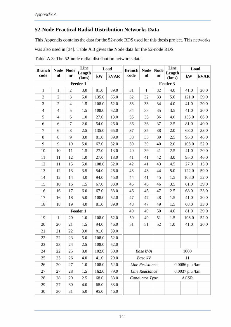
Appendix A
141
52-Node Practical Radial Distribution Networks Data
This Appendix contains the data for the 52-node RDS used for this thesis project. This networks
was also used in [34]. Table A.3 gives the Node data for the 52-node RDS.
Table A.3: The 52-node radial distribution networks data.
Branch code
Node nl
Node nr
Line Length (kms)
Load Branch
code Node
nl Node
nr
Line Length (kms)
Load
kW kVAR kW kVAR
Feeder 1 Feeder 3 1 1 2 3.0 81.0 39.0 31 1 32 4.0 41.0 20.0 2 2 3 5.0 135.0 65.0 32 32 33 5.0 121.0 59.0 3 2 4 1.5 108.0 52.0 33 33 34 4.0 41.0 20.0 4 4 5 1.5 108.0 52.0 34 33 35 3.5 41.0 20.0 5 4 6 1.0 27.0 13.0 35 35 36 4.0 135.0 66.0 6 6 7 2.0 54.0 26.0 36 36 37 2.5 81.0 40.0 7 6 8 2.5 135.0 65.0 37 35 38 2.0 68.0 33.0 8 8 9 3.0 81.0 39.0 38 33 39 2.5 95.0 46.0 9 9 10 5.0 67.0 32.0 39 39 40 2.0 108.0 52.0
10 10 11 1.5 27.0 13.0 40 39 41 2.5 41.0 20.0 11 11 12 1.0 27.0 13.0 41 41 42 3.0 95.0 46.0 12 11 15 5.0 108.0 52.0 42 41 43 4.5 27.0 13.0 13 12 13 3.5 54.0 26.0 43 43 44 5.0 122.0 59.0 14 12 14 4.0 94.0 45.0 44 41 45 1.5 108.0 52.0 15 10 16 1.5 67.0 33.0 45 45 46 3.5 81.0 39.0 16 16 17 6.0 67.0 33.0 46 45 47 2.5 68.0 33.0 17 16 18 5.0 108.0 52.0 47 47 48 1.5 41.0 20.0 18 18 19 4.0 81.0 39.0 48 47 49 1.5 68.0 33.0
Feeder 1 49 49 50 4.0 81.0 39.0 19 1 20 1.0 108.0 52.0 50 49 51 1.5 108.0 52.0 20 20 21 1.5 94.0 46.0 51 51 52 1.0 41.0 20.0 21 21 22 3.0 81.0 39.0 22 22 23 5.0 108.0 52.0 23 23 24 2.5 108.0 52.0 24 22 25 3.0 102.0 50.0 Base kVA 1000 25 25 26 4.0 41.0 20.0 Base kV 11 26 20 27 1.0 108.0 52.0 Line Resistance 0.0086 p.u./km 27 27 28 1.5 162.0 79.0 Line Reactance 0.0037 p.u./km 28 28 29 2.5 68.0 33.0 Conductor Type ACSR 29 27 30 4.0 68.0 33.0 30 30 31 5.0 95.0 46.0