Distributed Fault Detection for untimed and for timed Petri nets

1

Distributed Fault Detection

for untimed and for timed Petri nets

René Boel,

SYSTeMS Group, Ghent Universitywith thanks to:

G. Jiroveanu, G. Stremersch, B. Bordbar

2

Outline

• problem formulation and models

• centralised diagnosers via backward search

• distributed diagnosis for interacting Petri nets

• fault detection for timed Petri nets

• probabilistic fault diagnosis

3

adaptive supervisory control?

improve behaviour of large plants

consisting of many interacting components

controlled by disabling events

in order to guarantee that certain specifications are always satisfied

requires on-line estimation of current mode of operation of plant

4

feedback control paradigm

plant

observed output

state estimator

and fault detector

feedback law

controlled input

5

distributed feedback control paradigm

plant fault

detectorfeedback law

plant fault

detectorfeedback law

plantfault

detector

feedback law

plant fault detector

feedback law

6

distributed fault detection for large discrete event systems

• locally observable events at fault detection agenti (possibly small) subset of all events happening in planti

• assume: all observable events are always seen immediately by local fault detection (FD) agent, with their exact occurrence time (global clock)

7

distributed fault detection for large discrete event systems

• Can cooperation between local fault detection agents guarantee same quality of fault detection as would be achievable by a centralized fault detection agent that– observes all observable events (planti, i = 1,...,I)

– knows model of complete plant

• what is minimal information to be exchanged between FD agents for achieving same performance as centralized FD?

8

distributed state estimation for discrete event models

model includes unobservable events that cause deterioration of plant behavior, i.e. faults

each local fault detection agent implements local FD algorithm,

in order to adapt supervisor's reaction to current mode of operation of plant

local agent uses sequence of observable events generated locally

9

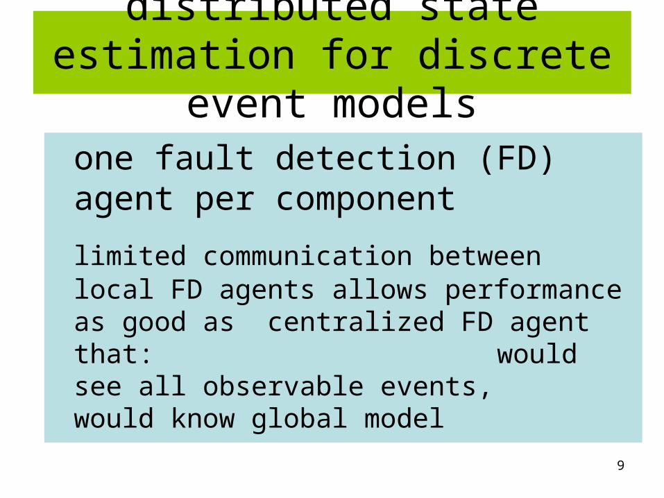
distributed state estimation for discrete event models

one fault detection (FD) agent per component

limited communication between local FD agents allows performance as good as centralized FD agent that: would see all observable events, would know global model

10

distributed observers

• distributed implementation reduces on-line computational complexity of FD agents

• distributed implementation makes fault detection more robust against communication errors that centralized FD

...provided local FD agents provide overestimate of set of possible faults

11


• distributed implementation of FD agents makes fault detection less sensitive to errors in knowledge about model

• especially knowledge of distant components often outdated when components change often

12


• but design more complicated because

– local FD agents must understand effects of interaction between components

– communication strategy between local FD agents must be designed

13

Petri net modelcommon places may be unobservable parts of physical network

interactions viacommon places -no common transitions

assume at least one observableevent in cycle covering more than one component

only very few transitions generate (locally)observable signal

14

interaction of Petri net components

• described by token passing via common places

• token entering boundary place enables events to happen only once in neighboring components

15


• described by token passing via common places

• token entering boundary place enables events to happen only once in neighboring components

16


• tight interaction between components

• local FD agenti may not know initial marking of places in planti

• forward explanations not possible for generation of allowed trajectories explaining observations

17

backward explanation

• generate all trajectories that

– are compatible with observations up to present time

– are compatible with plant model

• starting from most recently observed execution of transition t and recursively moving upward to its input places °t, its input transitions °(°t), and so on until possible previous marking is obtained

18

Petri net: example for explaining backward recursion

t13

places PP

transitions ΤΤ

Pre arc

Post arc

token

place with 2 tokens

19Algiers, 5/5/07 VECOS'07

decompose Petri net in 2 components that interact via places p5, p9

t13

each component contains one fault transition, resp. t1, t8

each component contains one observable transition,resp. t6, t10

20

observer design for one single component

• behaviour: Petri net model generates sequence of events

• observation: only some of the events are observed by control agent

• model: set T of transitions partitioned in observable transitions t To

and unobservable transitions t Tu

21

Petri net: compositional modelling

Large plants can be represented by several Petri net components, interacting with each other by unobservably exchanging tokens viacommon places

component 1 component 2

22


set P P of places of Petri net model consists of • "local places" in each component i

• for component i: "input places PPIN,i,jIN,i,j that have input transitions (Pre) in component j and output transitions (Post) in component i

• for component i: "output places PPOUT,i,jOUT,i,j that have output transitions (Pre) in component j and input transitions (Post) in component i

decomposition not constrained by limitations on decomposition not constrained by limitations on sensorssensors

23


To avoid unnecessary complications in analysis: assume Petri net bounded, i.e. all reachable markings have bounded number of tokens in each place

Problematic assumption: boundedness depends on the global structure of the Petri net, cannot be verified locally!

24


fault detection agenti for componenti

only observes local observable events

component 1 component 2

agent1 observes each occurrence of t6, at clock times (t6)n

agent2 observes each occurrence of t10

at clock times (t6)n

25

computational complexity

• combining two components of similar size leads to much more complicated behaviour

• number of possible traces of combination of two components is much larger than twice the size of the behaviour of each component separately!

• exponential explosion of computational complexity!

26

Outline


• why distributed on-line state estimation?

• backward generation of explanations

• distributed diagnosis

• extensions to timed DES models

• open questions and conclusions

27

example

p5 p8

p9

p11

p7

p6

t9

t8

t10

t11

t12

t13

only observable event: t10

fault event: t8

if only p8 is marked initially then only normal behaviour is trace {t12} and empty tracewhile possible faulty behaviour contains all prefixes of {t8, t10, t11}including empty trace

28

prefix

set of all prefixes of {t8, t10, t11}= , {t8}, {t8, t10}, {t8, t10, t11}

since untimed model does not specify any upper bound on time delays for events the model can never guarantee that an enabled event will have happened

29

example

p5 p8

p9

p11

p7

p6

t9

t8

t10

t11

t12

t13

only observable event: t10

fault event: t8

if only p5 is marked initially then normal behaviour includes all prefixes of the trace {t9, t13, t10, t11}where moreover t13 can alsooccur after t10 and after t11

30

unfolding of Petri net

• set of all prefixes and permissible reorderings of the trace {t9, t13, t10, t11}

= , {t9}, {t9, t13}, {t9, t10}, {t9, t13, t10},

{t9, t10, t13}, {t9, t10, t11}, {t9, t13, t10, t11},

{t9, t10, t13, t11}, {t9, t10, t11, t13}

• described by unfolding of the net, obtained by – by "opening all cycles" and – by "copying all places with more than 1 input

transition"

31

• example does not

contain cycles

• place p6 and place p9 must be replaced by 2, resp. 3 copies of the place


p5 p8

p9,1

p11

p7,2

p6,1

t9

t8

t11,1

t12

t13

p9,2 p9,3

p9,4

p7,1

p6,2t10,1

t11,2

t10,2

32

after unfolding a Petri net each token is generated by a uniquely defined sequence of events

problem: how to make an unfolding finite?

It is possible to obtain a finite unfolding of a Petri net so that "same behaviour" is generated (taking into account that repeating a cycle infinitely often does not generate new states)


33

forward analysis via unfolding

• if initial marking is known then one can enumerate all possible traces that end with an observable event occurrence

• and select as possible explanations of the observed events only those traces that contain the observed events in correct order

• using unfoldings avoids need for enumerating all possible orderings of unobservable events

34

forward analysis via unfolding

• but requirement that all initial markings are known (or an upper bound on these markings) is not acceptable for distributed fault detection

• since componenti does not know how many tokens componentj puts in input places PPIN,i,jIN,i,j and when it puts these tokens there

35

Outline


• why distributed on-line state estimation?

• centralised diagnosers


• extensions to timed DES models

• open questions and conclusions

36

backward search

• can avoid this difficulty

• finding minimal explanations via backward search determines where tokens should be available and by what time they must be in that place

37

example: backward search

p5 p8

p9

p11

p7

p6

t9

t8

t10

t11

t12

t13

observe: t10

at time (t10)

token must have arrived in p6

before (t10)

either fault t8 or unobservable event t9

must have fired before (t10)

38


p5 p8

p9

p11

p7

p6

t9

t8

t10

t11

t12

t13

observe: t10

at time (t10)

token must be present in p6 before (t10)or have been sent to p5 by neighboring component before (t10)

39


p5 p8

p9

p11

p7

p6

t9

t8

t10

t11

t12

t13

FD agent2 knows token was present in p8 prior to (t10) and hence it can determine that fault t8 may have occurred

but determining whether fault t8 occurred for sure requires information from neighboring component that it can put token in p5 before (t10)

40


p5 p8

p9

p11

p7

p6

t9

t8

t10

t11

t12

t13

in order to determine whether explanations (t9 t10) is also possible FD agent2 must ask niehgboring FD agent1

if it is possible that a token arrived in p5 before (t10)note that FD agent2 does not have to know model of plant1 except for fact that p5 is common place

41

possibility of token in p5

depends on whether•agent1 knows that 2 tokens in p0 present before (t10) if so then irrespective of how many times t6 has been observed by FD agent1 a token could may reach p5

prior to (t10)

VECOS'07Algiers, 5/5/07

t13


42

agent1 responds that it is possible that p5

became marked before time (t10)

from this response FD agent2 concludes that the fault t8 may or may not have

occurredVECOS'07Algiers, 5/5/07

t13


43

Note that a central observer knowing both models

and seeing all observations also would not be able to draw an unambiguous conclusion


t13


44

FD agent1 will return the same response if only 1 token is in p0 but t6 has not been observed yet, and the conclusion of FD agent2 will be the same however FD agent1 will know then that the token in p0 can no longer be used for future explanations


t13



t13


if only 1 token werepresent in p0 prior to (t10) and FD agent1 has observed the occurrence of t6 prior to (t10) then the token in p5 can only occur via (t0, t3, t6)which requires a token in p9 prior to (t10)


t13


but then ...agent1 must return the question to agent2 andask it is possible that p9 has received a token prior to (t10)FD agent2 will answer that this is indeed possible, and will receive a positive answer from FD agent1


t13


moreover FD agent2

knows that in that case the only explanation of t10 occurring at (t10)is the sequence of events(t9,t10)then FD agent2 can deduce that the fault t8 has not occurred

48

distributed fault diagnosis via backward search

• method described in simple example can be applied for all compositions of Petri nets interacting via common places

• using general algorithm for generating minimal explanations (backward unfolding)

• at random times any FD agent can initiate communication round that is assumed to reach a conclusion instantaneously (before any other fault or observable event can occur)

49

local explanation

= ordered sequence of local unobservable and observable events, so that

– ordering of observable events corresponds to observations

– uppermost transition of local explanation is either a place that is known locally to be marked initially, or a place where a token can enter the local component from a neighbouring component

50

fault diagnosis

• Relaxed diagnosis goal!• Enumerate only the minimal traces containing

sequences of events that must have happened for OBSOBSii to be allowable

• do not expand minimal traces, i.e. do not include transitions that do not lead to satisfaction of constraints necessary for occurrence of observable event

51

Minimal explanations

• Set ℇi,Min(OBSi ) of minimal local explanations using model of component i and local observations in model i

• would allows us – to decide if a fault happened for sure in

component i if we could detect the tokens entering via boundary places

52

Construction of minimal explanations

• assume OBS = OBS = {t1o}, 1st observation at time (t1

o)

• necessary constraint for execution of event t1o is

marking by at least 1 token of each place pink in

Pre(t1o)

• this in turn requires that for each place pink at least

one of the input transitions (determined by Post(., pin

k) of pink) has fired prior to (t1

o)

53

Construction of minimal explanations

• assumption no unobservable cycles with choice places sufficient to guarantee search stops in finite time

(ensures no problems occur due to tokens moving unobservably through cycles containing several initially marked places)

• all unobservable cycles must be trap circuits

54

faults should not be predictable

• theorem about equivalence of distributed and centralized diagnosis only true if reasonable assumption is made that faults are not predictable,

• i.e. there does not exist a marking that does inevitably lead to a fault transition

55

Some particularities of model

• Unlike many other distributed anayses (Fabre, Jard, Su,...)

• we assume global clock available• but each agent only knows local model and

interactions with neighbouring models• justification:

– GPS timer sufficiently accurate for applications, – but many reconfigurations make it difficult for

each agent to know global model– applications "slow" networks

56

distributed fault detection

• From time to time local agents should exchange enough information

• so that local diagnosis result in component i detects all the local faults that global diagnoser would detect at same time

• i.e. after communication between agents

local diagnosis = projection of global diagnosis

57

Outline


• why on-line state estimation?

• centralised diagnosers


• fault diagnosis for time Petri net models

• probabilistic DES, open questions and conclusions

58

timed discrete event models

• if minimal and maximal time delays for executing transitions are specified by model

• then not every untimed prefix of a possible trace is possible for timed model

• alternatively stated: adding a token may reduce reachable space

• analysis much more difficult, since set of reachable states not monotonely growing

• simplify notation: only 1-safe nets

59

time Petri net model

• assume t becomes enabled at p then t must be executed at some time [en(t) +L(t), en(t) +U(t)]

where en(t) = maxp●t {p}

• if t has not been executed yet, and no other enbabled transition has removed a token form one place in ●t, then t is forced to execute at en(t) +U(t)

60

time Petri net model

• consider choice place p with t1, t2 p●

if L(t2) > U(t1)

then t2 always pre-empted by t1

drop t2 from model

backward explanation of observations for timed model should remove such a path, even if it appears in explanation

for timed model

t1 t2

61

diagnosis can be refined by adding timing information to model

• start diagnosis for time Petri net model by developing, via backward search, set of minimal explanations of observations, compatible with untimed PN model

• check whether there exists for each event occurrence in untimed minimal explanation a non-empty interval of execution times that satisfies all the constraints

[en(t) +L(t), en(t) +U(t)]

62

• diagnosis for timed model starts with diagnosis for untimed model

• and then checks if there exists a legal valuation of all the event times in the untimed minimal explanation


63

• valuation of variables in set of linear inequalities = possible execution times of events in set of possible untimed explanations of observed events

• at time when observation occurs fix this execution time, and check if each element in set of explanations is still compatible with timed model


64

• for timed model also need to expand set of explanations forward since timed model may force events to happen by a certain and not observing such a forced event implies elimination of such an explanation from set of possible explanations


65

• need to recalculate set of solutions to conjunctive/disjunctive set of linear inequalities at each time when

– an observed event is executed

– an enabled unobservable transition is forced to occur

• reduce problem on real valued sets to finite state problem by using state classes of time Petri nets


66

• problem becomes further complicated if one takes into account that concurrently executed traces may be forced to remove a token from a place and thus may also eliminate a traces from set of possible explanations of an observed event


67

diagnosis for timed Petri nets

• variables in linear (in)equalities: execution times t of all events

t minimal explanation ℇMin(OBS ) of observed set OBS

• must satisfy equations:

min_explan/)(max)(min

)(max)(max

''

''

''''''''''''

''

TtU

UL

tttttt

ttttttttt

68

Outline

• problem formulation and models• why on-line state estimation?• centralised diagnosers • distributed diagnosis• extensions to timed DES models• probabilistic fault diagnosis, open questions

and conclusions

69

probabilistic diagnosis

• for free choice PNs it is possible to "easily" derive probability distribution over set of possible explanations of observed event sequence

• if t Tu: #(●t)=1 then it suffices to define for each place p a probability distribution over set of transitions in set p●

70


• if trace (t1 t2...tnO) {possible explanations}

of observation tnO at time (tn

O)

• and if pn = probability that token in unique place {pk} = ●tk moves to tk (i.e. pk = probability that tk is executed if pk becomes marked)

• then the weight of trace (t1 t2...tnO) in the of

possible explanations is k=1,...,n pk

71


• the probability of trace (t1 t2...tnO) in the of

possible explanations is obtained by normalizing these weights k=1,...,n pk over all elements in the set of explanations

• summing the probabilities of all traces that contain a fault defines the Bayesian (conditional) probability that the fault occurred, given the probabilistic model and given the observed sequence of events

72


• for free choice PNs need to assign probability per set of places in ●tj for set of concurrent transitions with common ●tj

• calculation remains largely identical then as before

• for non-free choice nets the compatible definition of the probabilities of choices made by tokens in places becomes very difficult

73

probabilitistic diagnosis of timed Petri nets

• timed petri nets where each firing time distribution is exponentially leads to Markov process (= stochastic PN)

• probababilistic diagnosis in principle easy (Bayesian recursive algorithm) in that case

• but set of explanations of sequence of observed events for stochastic PN = set of explanations of untimed PN

74

probabilitistic diagnosis of timed Petri nets

• combining forced transitions (= probability distribution over interval with finite upper bound) leads to very complicated analysis

• computational complexity probably same as using finite state abstraction of such a probabilistic PN

75

other case studies

• traffic modelling via hybrid systems

incident detection via failure diagnosis

• differences: – stochasticity much more important– really hybrid system: use fluid Petri nets or hybrid

automata– initial state belongs to large set of possible initial states

• concept of minimal explanation may be relevant in this case study too!

76

main ideas - open problems

• backward search more efficient/more easily distributed than forward search– for minimal explanations (faults that must have

occurred - diagnosis versus prognosis) – computational complexity– stopping criteria/saturated languages

• concurrency expressed via Petri nets• interaction between Petri net components via

common places

77

conclusions

• applying fault diagnosis to realistic plant model requires computationally efficient algorithms

• combine analysis of this talk with computer science approaches for describing large sets, and for reachability analysis

• abstraction leads to pessimistic fault detection results but may be inevitable

Documents

Distributed Fault Detection for untimed and for timed Petri nets