Embed Size (px)
Citation preview
ISSN 0280-5316 ISRN LUTFD2/TFRT--5883--SE
Distributed Control of Wind Farm
Benjamin Biegel
Department of Automatic Control Lund University
June 2011


Lund University Department of Automatic Control Box 118 SE-221 00 Lund Sweden
Document name
MASTER THESIS Date of issue
June 2011 Document Number
ISRN LUTFD2/TFRT--5883--SE Author(s)
Benjamin Biegel
Supervisor
Jakob Stoustrup Aalborg University, Denmark. Daria Madjidian Automatic Control Lund, Sweden. Anders Rantzer Automatic Control Lund, Sweden (Examiner) Sponsoring organization
Title and subtitle
Distributed Control of Wind Farm (Distribuerad reglering av vindkraftspark)
Abstract
The growing use of wind energy as major energy source, has led to the construction of large wind farms. The control of such wind farms is typically separated into control at wind turbine level and at wind farm level. The wind farm controller assures that the wind farm produces the demanded amount of power, by providing set-points for the turbines in the farm. The local turbine control assures that the local set-point is tracked. Current wind farm controllers conduct the power distribution in a static manner. In this work it is explored, how fatigue reduction in the wind farm can be achieved, by letting the controller distribute the power demand dynamically. In the first part of this work, the problem of reducing the fatigue on the turbines by dynamic power distribution is presented. A controller is designed based on this problem formulation, taking both tower and shaft fatigue into account. The controller is designed, such that it is both modular and scalable. This has the advantage of the controller being identical on all turbines in the wind farm. Also, the modularity allows turbines to be added or removed from the wind farm, without changing the controllers on the remaining turbines. Evaluation of the controller in a realistic simulation environment verifies the functionality of the controller, and shows that fatigue reductions of the tower and shaft in the magnitude of 10 % and 50 % respectively, can be expected. The final part of this work examines how the concept of fatigue reduction through dynamic wind farm control can be implemented on the offshore wind farm Thanet. Simulations indicate that the limitations of the server system at Thanet does not render this type of control possible.
Keywords
Classification system and/or index terms (if any)
Supplementary bibliographical information
ISSN and key title
0280-5316 ISBN
Language
English Number of pages
79 Recipient’s note
Security classification
http://www.control.lth.se/publications/


Preface
This thesis is the result of my 10th semester at Aalborg University. The project has been con-ducted as a study abroad at Lund University in Lund, Sweden.
The work consists of this thesis along with an appended CD.
I owe my supervisor, prof. Jakob Stoustrup great thanks for his support through the course ofthe semester, and especially for setting up the connection to Lund University. I also give greatthanks to all the people at Lund University, who have made the stay at Lund University possible.Anders Rantzer and Daria Madjidian for many hours of support through the project, and forincluding me in the Aeolus experiments. Eva Westin for helping with all practical aspects andfor finding an apartment in Lund.
Also I want to thank Joachim Løvgaard, for designing the beautiful cover pages.
Finally, I want to thank Siemens A/S Fond and Otto Mønsteds Fond, for supporting my studiesfinancially.

Contents
1 Introduction 7
2 Overview 8
2.1 Wind Farm Control . . . . . . . . . . . . . . . . . . . . . . . . . . . . . . . . . . . 8
2.2 Distributed Control . . . . . . . . . . . . . . . . . . . . . . . . . . . . . . . . . . . . 10
2.3 Thesis Overview . . . . . . . . . . . . . . . . . . . . . . . . . . . . . . . . . . . . . 11
I Modular Distributed Wind Farm Control 14
3 Outline Part I 15
4 Modeling 16
4.1 Wind Turbine Model . . . . . . . . . . . . . . . . . . . . . . . . . . . . . . . . . . . 16
4.2 Wind Farm Model . . . . . . . . . . . . . . . . . . . . . . . . . . . . . . . . . . . . 21
4.3 Wind Model . . . . . . . . . . . . . . . . . . . . . . . . . . . . . . . . . . . . . . . . 22
4.4 Fatigue Model . . . . . . . . . . . . . . . . . . . . . . . . . . . . . . . . . . . . . . . 23
5 Wind Farm Problem Formulation 25
5.1 Initial Problem Formulation . . . . . . . . . . . . . . . . . . . . . . . . . . . . . . . 25
5.2 Linear Wind Farm Description . . . . . . . . . . . . . . . . . . . . . . . . . . . . . 27
5.3 Quadratic Fatigue Description . . . . . . . . . . . . . . . . . . . . . . . . . . . . . . 30
5.4 Quadratic Problem Formulation . . . . . . . . . . . . . . . . . . . . . . . . . . . . . 34
6 Modular Distributed Wind Farm Controller 37
6.1 Iterative State Feedback . . . . . . . . . . . . . . . . . . . . . . . . . . . . . . . . . 37
6.2 Distributed Synthesis . . . . . . . . . . . . . . . . . . . . . . . . . . . . . . . . . . . 38
6.3 Control Algorithm . . . . . . . . . . . . . . . . . . . . . . . . . . . . . . . . . . . . 43
6.4 Alternative Algorithms . . . . . . . . . . . . . . . . . . . . . . . . . . . . . . . . . . 44
7 Controller Performance Evaluation 48
7.1 Evaluation in Linear Wind Farm . . . . . . . . . . . . . . . . . . . . . . . . . . . . 48
7.2 Evaluation in NREL Wind Farm . . . . . . . . . . . . . . . . . . . . . . . . . . . . 51
5 of 79
CONTENTS
II Distributed Controller for Thanet Wind Farm 55
8 Outline Part II 56
9 Thanet Wind Farm Experiment Description 57
9.1 Experiment Goal . . . . . . . . . . . . . . . . . . . . . . . . . . . . . . . . . . . . . 57
9.2 Experiment Setup . . . . . . . . . . . . . . . . . . . . . . . . . . . . . . . . . . . . 57
9.3 System Limitations . . . . . . . . . . . . . . . . . . . . . . . . . . . . . . . . . . . . 58
10 Control Strategy 60
10.1 Simplified Distributed Wind Farm Controller . . . . . . . . . . . . . . . . . . . . . 60
10.2 Distribution of Controller . . . . . . . . . . . . . . . . . . . . . . . . . . . . . . . . 61
10.3 Control Objective . . . . . . . . . . . . . . . . . . . . . . . . . . . . . . . . . . . . . 62
10.4 Linear Quadratic Control . . . . . . . . . . . . . . . . . . . . . . . . . . . . . . . . 63
11 Controller Design and Evaluation 64
11.1 Problem Formulation . . . . . . . . . . . . . . . . . . . . . . . . . . . . . . . . . . . 64
11.2 Accommodating System Limitations . . . . . . . . . . . . . . . . . . . . . . . . . . 65
11.3 Controller Design . . . . . . . . . . . . . . . . . . . . . . . . . . . . . . . . . . . . . 66
11.4 Performance Evaluation . . . . . . . . . . . . . . . . . . . . . . . . . . . . . . . . . 67
III Epilogue 69
12 Conclusion 70
12.1 Modular Distributed Wind Farm Control . . . . . . . . . . . . . . . . . . . . . . . 70
12.2 Distributed Controller for Thanet Wind Farm . . . . . . . . . . . . . . . . . . . . . 71
A Rainflow Counting Algorithm 72
B List of Acronyms 74
Bibliography 75
6 of 79 CONTENTS
Chapter 1
Introduction
The earth’s fossil energy resources are limited and large resistance exists towards the use ofnuclear power plants, supported by recent events. This calls for alternative ways of meeting theworld’s increasing need of power. Renewable energy is expected to play a big role in solving thisproblem [Sti08], [Bul01].
With an exponential growth over a long period of years, wind energy is a promising source ofrenewable energy [Sti08]. A large amount of research in the area of wind turbine control hastherefore been conducted. The typical focus of this research is power production maximization,power quality optimization, and fatigue minimization, see e.g. [BSJB01], [WWB10], [NCVT10],[XXZ+08], [JPP08], [BJS+11].
For economic reasons, it is desirable to place wind turbines close to each other. This has led tothe construction of wind farms, where large numbers of wind turbines operate together to meetsome total power demand. The control of such wind farms is the topic of this thesis.
The wind farm control must assure, that the wind turbines in the farm produce the demandedpower. This is accomplished by distributing the total power demand among the turbines in thewind farm, by providing each turbine with a power set-point. The turbines in the farm then usetheir local wind turbine controller to track this power set-point.
When the wind farm power demand is less than the available power, the controller is free todistribute the power set-points among the turbines, as long as the farm power demand is met.This introduces a freedom in the wind farm control. In current wind farms this freedom is notexploited, as the power distribution is done in a static manner based on long term measurementsand predictions [KBS09], [HSBF05]. The focus of this thesis is to benefit from this freedom, bydesigning a wind farm controller that reduces the fatigue on the turbines in the wind farm, whilemeeting the farm power demand.
The first part of the thesis is based on a modular control strategy developed in [MMR11]. Thecontrol strategy achieves wind farm fatigue minimization by dynamically changing the powerproduction set-points of the turbines in the wind farm. This is done in a distributed manner,based on communication between neighboring turbines in the wind farm. In this work, thismethod is described, modified and evaluated through realistic wind farm simulations.
In the second part, the focus is the development of a controller suitable for real wind farmexperiments. These experiments are planned to be performed at Thanet wind farm in the UK inthe summer of 2011. As the wind turbines at Thanet are not constructed with dynamic controlin mind, the turbines only offer a limited possibility to apply this type of control, which must betaken into account in the controller design. Based on these limitations, a controller is designedand evaluated through simulations.
7 of 79
Chapter 2
Overview
In this chapter, the concepts of wind farm control and distributed control are introduced. Further,
this chapter describes the scope of the two parts of this work. The first part concerns modular
distributed controller design, while the subject of the second part is a distributed controller designed
for Thanet wind farm.
2.1 Wind Farm Control
Wind Farm Control Overview
In a wind farm, a large number of wind turbines are positioned close to each other. The controlof such a wind farm is illustrated in Figure 2.1. The turbines in the wind farm are illustrated tothe right, each producing the power P i
out, thus producing a total power of Pfarm,out =∑N
i=1 Piout,
where N is the number of turbines. Also, each turbine experiences some measure of fatigueJ i, which means that the total fatigue in the farm becomes Jfarm =
∑Ni=1 J
i. The fatigue candescribe the mechanical loads on the turbines, the quality of the power, etc.
The control of the wind farm is split up into farm level control and turbine level control. Thewind farm control distributes power set-points to all the turbines in the farm, i.e. turbine i isgiven the set-point P i
dem etc. The local turbine controller in each wind turbine ensures that theoutput power of turbine P i
out tracks the given power set-point P idem. At the same time, the local
wind turbine controller seeks other objectives, e.g. ensures structural stability.
As illustrated by 2.1, the wind farm controller distributes the power set-points P idem based on the
power demand to the whole wind farm Pfarm,dem. Also various measurements from the turbinesin the farm ymeas,i, and often also from a meteorological mast, are available to the wind farmcontroller.
Currently the wind farm controller determines the power set-points P idem based on wind measure-
ments in the wind farm and on long term wind predictions. Based on these and the demand tothe whole wind farm Pfarm,dem, the wind farm controller provides static power set-points to allthe turbines in the farm.
In this work we examine how to exploit the freedom in choosing the power set-points dynamically,such that the fatigue on the turbines in the wind farm is reduced, while honoring the powerdemand of the network operator.
By the terminology of Figure 2.1, we can roughly state that the current wind farm controllersensure that Pfarm,out = Pfarm,dem by static power distribution. In this work, we seek to use
8 of 79
2.1. WIND FARM CONTROL
Pfarm,available
Pfarm,demP idem
ymeas,i
Pfarm,out
Jfarm
Wind farmcontroller
NetworkOperator
Wind farmturbines
Figure 2.1: Illustration of a wind farm controller, operating based on measurements and onthe power demanded by the network operator. The figure is based on [KBS09].
feedback to control the power set-points P idem dynamically, leading to a minimization of Jfarm,
while still ensuring that Pfarm,out = Pfarm,dem.
Wind Farm Control Illustration
To illustrate the concept of a wind turbine control, the following simple fictive example is con-sidered.
A wind farm consisting of five wind turbines is controlled by a wind farm controller. This iscurrently very roughly done in the following manner. Based on measurements from each windturbine, the total available power in the farm can be determined. If there is more power availablethan demanded, each turbine is asked to generate a fraction of the power available to the giventurbine.
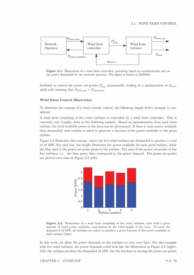
Figure 2.2 illustrates this concept, where the five wind turbines are demanded to produce a totalof 10 MW. For each bar, the height illustrates the power available for each given turbine, whilethe blue part is the power set-point given to the turbine. The sum of the power set-points of thefive turbines, i.e. the blue parts, then correspond to the power demand. The power set-pointsare plotted over time in Figure 2.3 (left).
Pow
er[M
W]
Turbine number1 2 3 4 5
0
0.5
1
1.5
2
2.5
3
Figure 2.2: Illustration of a wind farm consisting of five wind turbines, each with a givenamount of wind power available, represented by the total height of the bars. To meet thedemand of 10 MW, all turbines are asked to produce a given fraction of the power available ateach turbine (blue).
In this work, we allow the power demands to the turbines to vary over time. For this examplewith five wind turbines, the power demands could look like the illustration in Figure 2.3 (right).Still, the turbines produce the demanded 10 MW, but the freedom in varying the power set-points
CHAPTER 2. OVERVIEW 9 of 79
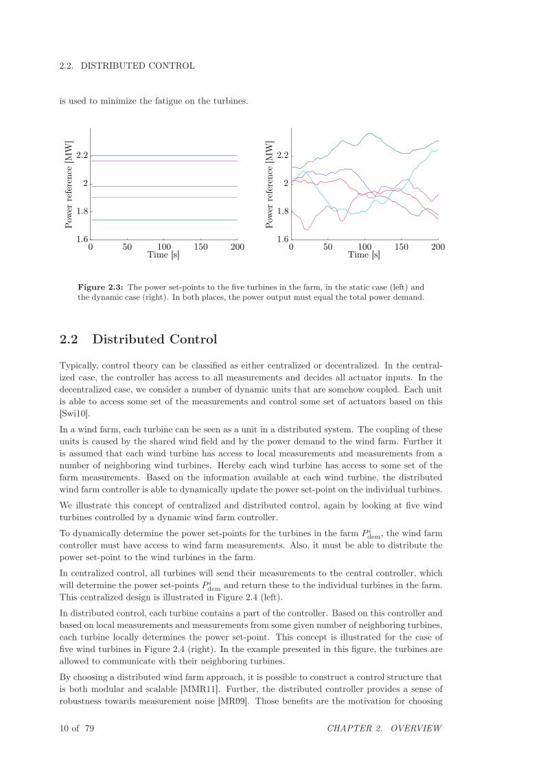
2.2. DISTRIBUTED CONTROL
is used to minimize the fatigue on the turbines.
Pow
erre
fere
nce
[MW
]
Time [s]0 50 100 150 200
1.6
1.8
2
2.2
Pow
erre
fere
nce
[MW
]
Time [s]0 50 100 150 200
1.6
1.8
2
2.2
Figure 2.3: The power set-points to the five turbines in the farm, in the static case (left) andthe dynamic case (right). In both places, the power output must equal the total power demand.
2.2 Distributed Control
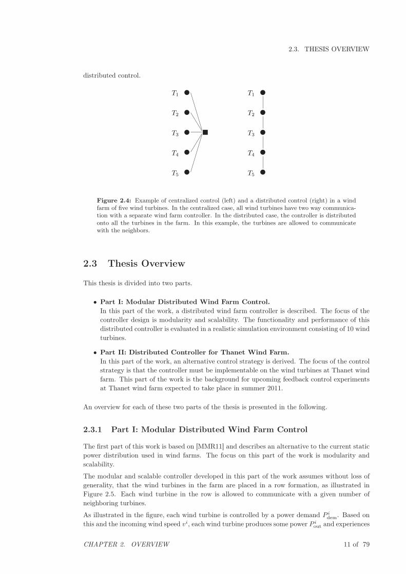
Typically, control theory can be classified as either centralized or decentralized. In the central-ized case, the controller has access to all measurements and decides all actuator inputs. In thedecentralized case, we consider a number of dynamic units that are somehow coupled. Each unitis able to access some set of the measurements and control some set of actuators based on this[Swi10].
In a wind farm, each turbine can be seen as a unit in a distributed system. The coupling of theseunits is caused by the shared wind field and by the power demand to the wind farm. Further itis assumed that each wind turbine has access to local measurements and measurements from anumber of neighboring wind turbines. Hereby each wind turbine has access to some set of thefarm measurements. Based on the information available at each wind turbine, the distributedwind farm controller is able to dynamically update the power set-point on the individual turbines.
We illustrate this concept of centralized and distributed control, again by looking at five windturbines controlled by a dynamic wind farm controller.
To dynamically determine the power set-points for the turbines in the farm P idem, the wind farm
controller must have access to wind farm measurements. Also, it must be able to distribute thepower set-point to the wind turbines in the farm.
In centralized control, all turbines will send their measurements to the central controller, whichwill determine the power set-points P i
dem and return these to the individual turbines in the farm.This centralized design is illustrated in Figure 2.4 (left).
In distributed control, each turbine contains a part of the controller. Based on this controller andbased on local measurements and measurements from some given number of neighboring turbines,each turbine locally determines the power set-point. This concept is illustrated for the case offive wind turbines in Figure 2.4 (right). In the example presented in this figure, the turbines areallowed to communicate with their neighboring turbines.
By choosing a distributed wind farm approach, it is possible to construct a control structure thatis both modular and scalable [MMR11]. Further, the distributed controller provides a sense ofrobustness towards measurement noise [MR09]. Those benefits are the motivation for choosing
10 of 79 CHAPTER 2. OVERVIEW
2.3. THESIS OVERVIEW
distributed control.
T1
T2
T3
T4
T5
T1
T2
T3
T4
T5
Figure 2.4: Example of centralized control (left) and a distributed control (right) in a windfarm of five wind turbines. In the centralized case, all wind turbines have two way communica-tion with a separate wind farm controller. In the distributed case, the controller is distributedonto all the turbines in the farm. In this example, the turbines are allowed to communicatewith the neighbors.
2.3 Thesis Overview
This thesis is divided into two parts.
• Part I: Modular Distributed Wind Farm Control.
In this part of the work, a distributed wind farm controller is described. The focus of thecontroller design is modularity and scalability. The functionality and performance of thisdistributed controller is evaluated in a realistic simulation environment consisting of 10 windturbines.
• Part II: Distributed Controller for Thanet Wind Farm.
In this part of the work, an alternative control strategy is derived. The focus of the controlstrategy is that the controller must be implementable on the wind turbines at Thanet windfarm. This part of the work is the background for upcoming feedback control experimentsat Thanet wind farm expected to take place in summer 2011.
An overview for each of these two parts of the thesis is presented in the following.
2.3.1 Part I: Modular Distributed Wind Farm Control
The first part of this work is based on [MMR11] and describes an alternative to the current staticpower distribution used in wind farms. The focus on this part of the work is modularity andscalability.
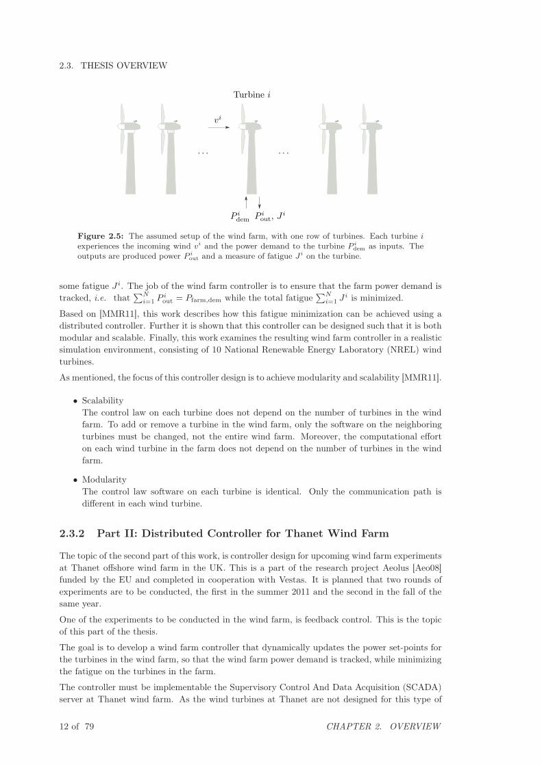
The modular and scalable controller developed in this part of the work assumes without loss ofgenerality, that the wind turbines in the farm are placed in a row formation, as illustrated inFigure 2.5. Each wind turbine in the row is allowed to communicate with a given number ofneighboring turbines.
As illustrated in the figure, each wind turbine is controlled by a power demand P idem. Based on
this and the incoming wind speed vi, each wind turbine produces some power P iout and experiences
CHAPTER 2. OVERVIEW 11 of 79
2.3. THESIS OVERVIEW
. . . . . .
vi
Turbine i
P idem P i
out, Ji
Figure 2.5: The assumed setup of the wind farm, with one row of turbines. Each turbine i
experiences the incoming wind vi and the power demand to the turbine P i
dem as inputs. Theoutputs are produced power P i
out and a measure of fatigue J i on the turbine.
some fatigue J i. The job of the wind farm controller is to ensure that the farm power demand istracked, i.e. that
∑Ni=1 P
iout = Pfarm,dem while the total fatigue
∑Ni=1 J
i is minimized.
Based on [MMR11], this work describes how this fatigue minimization can be achieved using adistributed controller. Further it is shown that this controller can be designed such that it is bothmodular and scalable. Finally, this work examines the resulting wind farm controller in a realisticsimulation environment, consisting of 10 National Renewable Energy Laboratory (NREL) windturbines.
As mentioned, the focus of this controller design is to achieve modularity and scalability [MMR11].
• ScalabilityThe control law on each turbine does not depend on the number of turbines in the windfarm. To add or remove a turbine in the wind farm, only the software on the neighboringturbines must be changed, not the entire wind farm. Moreover, the computational efforton each wind turbine in the farm does not depend on the number of turbines in the windfarm.
• ModularityThe control law software on each turbine is identical. Only the communication path isdifferent in each wind turbine.
2.3.2 Part II: Distributed Controller for Thanet Wind Farm
The topic of the second part of this work, is controller design for upcoming wind farm experimentsat Thanet offshore wind farm in the UK. This is a part of the research project Aeolus [Aeo08]funded by the EU and completed in cooperation with Vestas. It is planned that two rounds ofexperiments are to be conducted, the first in the summer 2011 and the second in the fall of thesame year.
One of the experiments to be conducted in the wind farm, is feedback control. This is the topicof this part of the thesis.
The goal is to develop a wind farm controller that dynamically updates the power set-points forthe turbines in the wind farm, so that the wind farm power demand is tracked, while minimizingthe fatigue on the turbines in the farm.
The controller must be implementable the Supervisory Control And Data Acquisition (SCADA)server at Thanet wind farm. As the wind turbines at Thanet are not designed for this type of
12 of 79 CHAPTER 2. OVERVIEW
2.3. THESIS OVERVIEW
control, some very strict limitations are present.
For this reason, the focus on this second part of the work is to examine and accommodate thelimitations of the SCADA server. Further it is desired that the controller is simplified as muchas possible, while still illustrating the benefit of wind farm control.
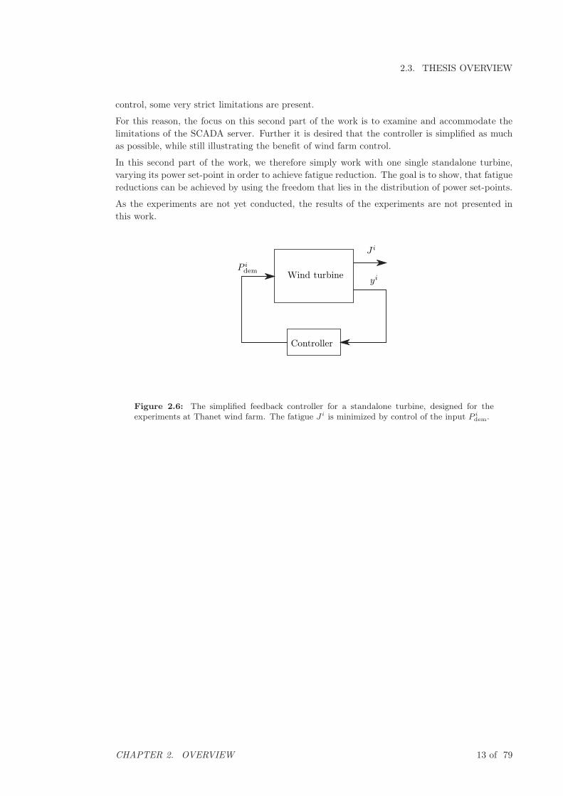
In this second part of the work, we therefore simply work with one single standalone turbine,varying its power set-point in order to achieve fatigue reduction. The goal is to show, that fatiguereductions can be achieved by using the freedom that lies in the distribution of power set-points.
As the experiments are not yet conducted, the results of the experiments are not presented inthis work.
Wind turbineyi
P idem
J i
Controller
Figure 2.6: The simplified feedback controller for a standalone turbine, designed for theexperiments at Thanet wind farm. The fatigue J i is minimized by control of the input P i
dem.
CHAPTER 2. OVERVIEW 13 of 79
Part I
Modular Distributed Wind Farm
Control
14 of 79

Chapter 3
Outline Part I
This chapter describes the outline of this first part of the Thesis. This part of the work modifies
and evaluates the wind farm controller described in [MMR11].
• Modeling, Chapter 4This chapter describes how a dynamic wind farm model is obtained for a farm consistingof a number of National Renewable Energy Laboratory (NREL) wind turbines. Further itis examined how wind turbine fatigue can be modeled.
• Wind Farm Problem Formulation, Chapter 5This chapter describes how a linear wind turbine model can be obtained through lineariza-tion of the dynamic non-linear wind turbine model. Similarly it is described, how a quadraticfunction can be used to describe the wind turbine fatigue.
• Modular Distributed Wind Farm Controller, Chapter 6This chapter describes how a modular and scalable wind farm controller can be developedbased on the linearized model, and by letting the wind turbines communicate with a limitednumber of neighbors.
• Controller Performance Evaluation, Chapter 7This chapter evaluates the performance of the modular and scalable wind farm controller,by simulating the performance in a wind farm consisting of 10 NREL wind turbines.
15 of 79

Chapter 4
Modeling
This chapter seeks to construct a model of a wind farm, useful for controller design. This includes
wind turbine modeling, wind field modeling and fatigue modeling.
4.1 Wind Turbine Model
This section describes the wind turbine used as basis of the controller design throughout thefollowing chapters.
4.1.1 The NREL Wind Turbine
It is chosen to base the wind farm controller design and later simulations, on the National Re-
newable Energy Laboratory (NREL) offshore 5-MW baseline wind turbine. A thorough model ofthis wind turbine has been constructed and is available [JBMS09], along with simplifications ofthe model [SJBMV07], [GSK+10]. The motivation for choosing this model as vantage point forthe controller design, is that this model is designed to be representative of typical land- and seabased multimegawatt turbines [JBMS09].
Note further, that it is trivial to design the controller for another type of wind turbines, simplyby replacing the NREL model in the controller design phase.
The NREL wind turbine, is a 5 MW variable speed offshore wind turbine with active hydraulicpitch control. In the following, an overview will be given of the NREL wind turbine, to provide thenecessary understanding of the dynamics of the wind turbine. Note that this model is presentedon an overview level, as the focus of this work is wind farm control rather than wind farmmodeling. For more detail on the model of the NREL wind turbine, refer to [JBMS09]. Alsonote, that [SJBMV07] is the background for the modeling of the NREL wind turbine.
Note that the following model description, including data, is taken from [SJBMV07], [JBMS09],[Aeo10b] and [Aeo10a]. Parts of the scripts used in the sequel are likewise provided by the authorsof [SJBMV07]. All source code is found in the enclosed CD, and the paths to the different scripsare presented in the following.
4.1.2 Model Purpose
The purpose of the model of the wind turbine, is to achieve a model useful for controller designat wind farm level. The model we are seeking is thus a closed loop wind turbine model with a
16 of 79
4.1. WIND TURBINE MODEL
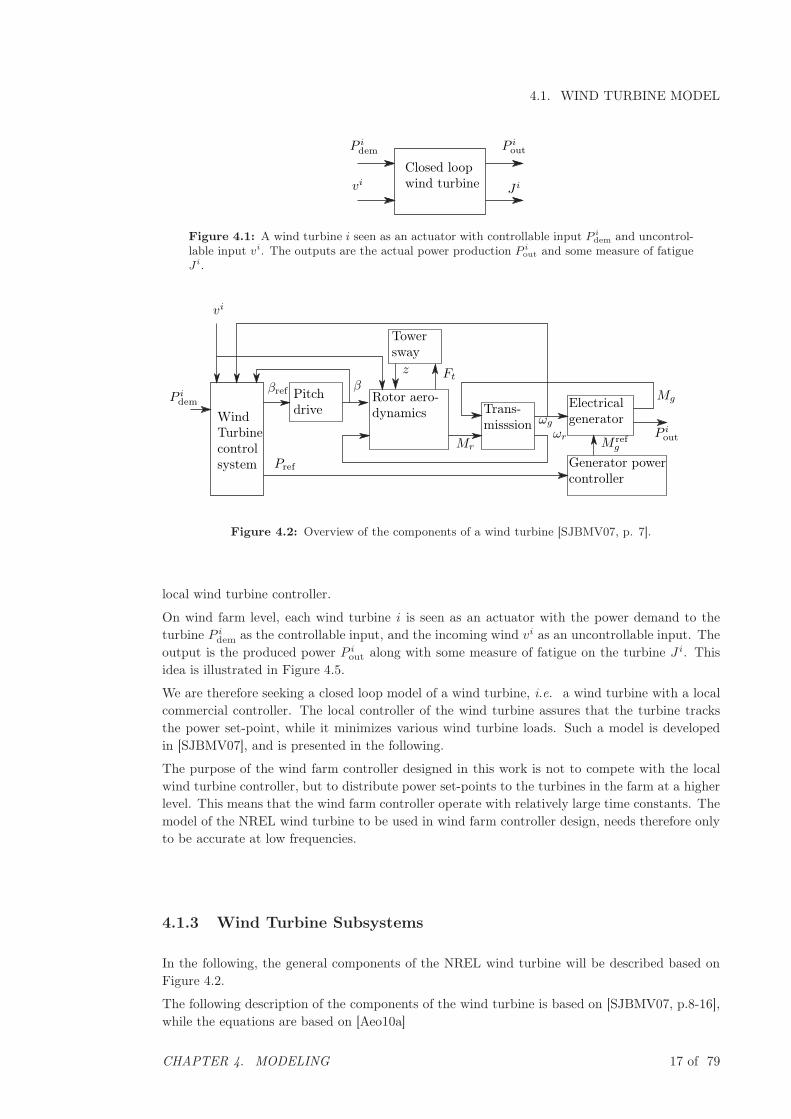
Closed loopwind turbine J ivi
P idem P i
out
Figure 4.1: A wind turbine i seen as an actuator with controllable input P i
dem and uncontrol-lable input vi. The outputs are the actual power production P i
out and some measure of fatigueJ i.
WindTurbinecontrolsystem
P idem
Pitchdrive
Towersway
Electricalgenerator
Generator powercontroller
Mr
ωr
ωgP iout
Mg
M refg
Ftz
ββref
vi
Pref
Rotor aero-dynamics Trans-
misssion
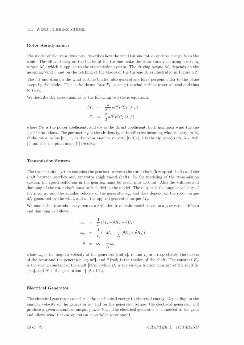
Figure 4.2: Overview of the components of a wind turbine [SJBMV07, p. 7].
local wind turbine controller.
On wind farm level, each wind turbine i is seen as an actuator with the power demand to theturbine P i
dem as the controllable input, and the incoming wind vi as an uncontrollable input. Theoutput is the produced power P i
out along with some measure of fatigue on the turbine J i. Thisidea is illustrated in Figure 4.5.
We are therefore seeking a closed loop model of a wind turbine, i.e. a wind turbine with a localcommercial controller. The local controller of the wind turbine assures that the turbine tracksthe power set-point, while it minimizes various wind turbine loads. Such a model is developedin [SJBMV07], and is presented in the following.
The purpose of the wind farm controller designed in this work is not to compete with the localwind turbine controller, but to distribute power set-points to the turbines in the farm at a higherlevel. This means that the wind farm controller operate with relatively large time constants. Themodel of the NREL wind turbine to be used in wind farm controller design, needs therefore onlyto be accurate at low frequencies.
4.1.3 Wind Turbine Subsystems
In the following, the general components of the NREL wind turbine will be described based onFigure 4.2.
The following description of the components of the wind turbine is based on [SJBMV07, p.8-16],while the equations are based on [Aeo10a]
CHAPTER 4. MODELING 17 of 79
4.1. WIND TURBINE MODEL
Rotor Aerodynamics
The model of the rotor dynamics, describes how the wind turbine rotor captures energy from thewind. The lift and drag on the blades of the turbine make the rotor turn generating a drivingtorque Ms, which is applied to the transmission system. The driving torque Ms depends on theincoming wind v and on the pitching of the blades of the turbine β, as illustrated in Figure 4.2.
The lift and drag on the wind turbine blades, also generates a force perpendicular to the planeswept by the blades. This is the thrust force Ft, causing the wind turbine tower to bend and thusto sway.
We describe the aerodynamics by the following two static equations.
Ms =π
2ωrρR2v3CP (λ, β)
Ft =π
2ρR2v2CT (λ, β)
where CP is the power coefficient, and CT is the thrust coefficient, both nonlinear wind turbinespecific functions. The parameter ρ is the air density, v the effective incoming wind velocity [m/s],R the rotor radius [m], wr is the rotor angular velocity [rad/s], λ is the tip speed ratio λ = ωrR
v
[-] and β is the pitch angle [◦] [Aeo10a].
Transmission System
The transmission system contains the gearbox between the rotor shaft (low speed shaft) and theshaft between gearbox and generator (high speed shaft). In the modeling of the transmissionsystem, the speed reduction in the gearbox must be taken into account. Also the stiffness anddamping of the rotor shaft must be included in the model. The output is the angular velocity ofthe rotor ωr and the angular velocity of the generator ωg, and they depend on the rotor torqueMs generated by the wind, and on the applied generator torque Mg.
We model the transmission system as a 3rd oder drive train model based on a gear ratio, stiffnessand damping as follows.
ωr =1
Ir(Ms − θKs − θBs)
ωg =1
Ig(−Mg +
1
N(θKs + θBs))
θ = ωr −1
Nωg
where ωg is the angular velocity of the generator [rad/s], Ir and Ig are, respectively, the inertiaof the rotor and the generator [kg/m2], and θ [rad] is the torsion of the shaft. The constant Ks
is the spring constant of the shaft [N/m], while Bs is the viscous friction constant of the shaft [Ns/m], and N is the gear ration [-] [Aeo10a].
Electrical Generator
The electrical generator transforms the mechanical energy to electrical energy. Depending on theangular velocity of the generator ωg and on the generator torque, the electrical generator willproduce a given amount of output power Pout. The electrical generator is connected to the grid,and allows wind turbine operation at variable rotor speed.
18 of 79 CHAPTER 4. MODELING

4.1. WIND TURBINE MODEL
Generator Power Controller
The generator power controller makes the wind turbine track the power set-point P idem by con-
trolling the reference signal for the turbine generator torque M refg . By increasing the generator
torque Mg, the power production will increase, while the angular velocity will remain the same.
We describe the electrical generator together with the generator power controller as a 1st ordermodel with the input being Pref. In other words, we do not model the generator torque referenceM ref
g explicitly. We use the following model.
Mg =1
τg
(Pref
ωg−Mg
)
where τg is the generator time constant [s] [Aeo10a].
Tower Sway
The thrust force caused by the wind on the rotors, will excite the wind turbine tower. This willlead to an undesired nodding of the tower, producing fatigue to the wind turbine. Also, thisnodding affects the rotor dynamics, as the relative wind speed will change as the turbine moves.It is a task of the local wind turbine controller, to minimize this tower sway.
We model the tower deflection pnac [m], corresponding to the nacelle position, as a spring damper-system as follows.
pnac =1
mt(Ft −Ktpnac −Btpnac)
where mt is the mass of the tower and Kt and Bt are, respectively, the spring and damperconstants of the tower [Aeo10a].
Pitch Drive
In the NREL wind turbine, the actuators are hydraulic pitch actuators, with some given band-width. Therefore the pitch drive dynamics must be included in the wind turbine model, as thepath from the pitch reference βref to the pitch angle of the blades β is characterized by a delay,first order filter characteristics and quantization.
The pitch drive is modeled as a second order system with a time constant τβ and an input delaytβ , closed loop with a proportional controller with constant Kβ.
β =1
τβ(uβe
−tβs/s− β)
uβ = Kβ(βref − βmeas)
where βmeas is the measurement of the pitch [◦] [Aeo10a].
Wind Turbine Controller
The two inputs considered to the wind turbine, is the effective wind velocity vi and the powerdemand P i
dem. Here P idem is the control variable of the wind farm controller designed in this
work. The goal of the local wind turbine controller is to ensure that power set-point is tracked,i.e. that P i
out = P idem. When the power demand is not achievable, due to too low available power
in the wind, the wind turbine controller must maximize the power production. This reveals twodifferent modes of the wind turbine, power maximization and power tracking. We notice, that in
CHAPTER 4. MODELING 19 of 79
4.1. WIND TURBINE MODEL
the power maximization mode, the wind turbine no longer acts as an actuator through P idem, but
solely tries to maximize the output power P iout.
The local wind turbine controller must additionally guarantee, that the turbine obeys the givenconstraints to the wind turbine, e.g. the speed and torque on the generator. Similarly, thelocal wind turbine controller must reduce the fatigue on the wind turbine, by damping the windturbine tower bending and the shaft torsion.
It is worth noticing, that two internal control variables are the wind turbine pitch β and thereference to the generator torque M ref
g , which provides the freedom to control the wind turbinein a desired manner.
The behavior in the two different control regions is.
• Power Maximization. In the power maximization, the pitch reference is zero βref = 0. Atthe same time, the generator torque reference is affected through the power reference Pref ,to maximize the power output P i
out. The wind turbine controller does this by measuringthe generator angular velocity ωg, and by looking up the optimal generator torque Mg forthe given angular velocity ωg, and modifying Pref accordingly.
• Power Tracking. In the power tracking mode, the wind turbine controller makes the windturbine generator rotate with the nominal angular velocity ωg = ωnom
g , by measurements ofωg and utilization of the pitch actuator, through β. It corrects the power set-point P i
dem tocompensate for transmission losses, and provides it as the power reference Pref .
The controller is implemented in the following way. In the power maximization region, the powerreference Pref is simply found in a look-up table dependent on the generator angular velocity ωg,while the pitch is kept constant at zero.
In the power tracking region, the generator power is kept constant at the desired power, whilethe turbine is brought to rotate with the nominal angular velocity using the blade pitching. Thiscontrol system is implemented with a gain scheduled PI controller as follows.
βref = KP (β)ωe +KI(β)
∫ t
0
ωedt
KP (β) = KP,0(β)β2
β2 + β
KI(β) = KI,0(β)β2
β2 + β
where ωe is the error between the desired angular velocity of the generator, and the actualangular velocity of the generator. The proportional and integral gains KP and KI are based onthe proportional and integral base gains KP,0 and KI,0 when there is no pitching β = 0, whilethe parameter β2 is the pitch angle where the pitch sensitivity is doubled [Aeo10a].
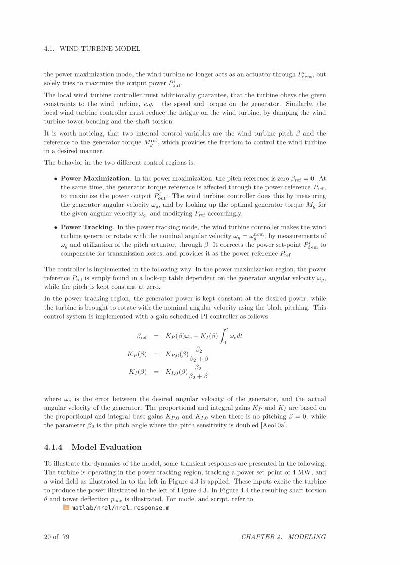
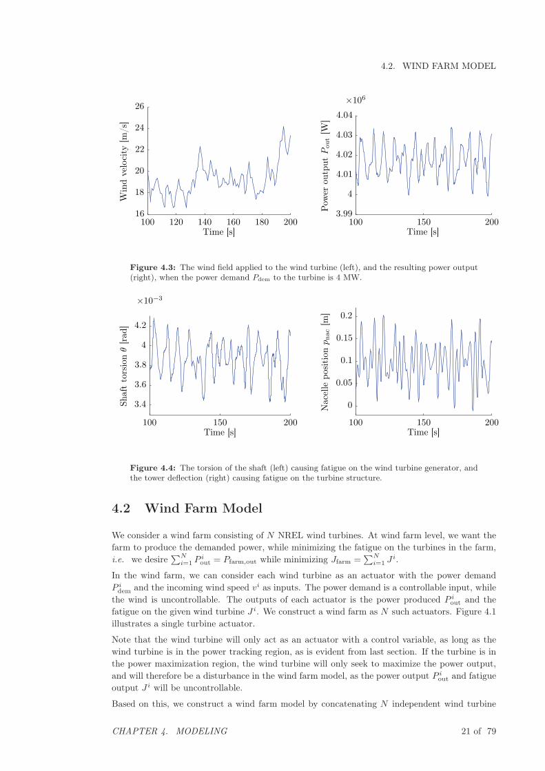
4.1.4 Model Evaluation
To illustrate the dynamics of the model, some transient responses are presented in the following.The turbine is operating in the power tracking region, tracking a power set-point of 4 MW, anda wind field as illustrated in to the left in Figure 4.3 is applied. These inputs excite the turbineto produce the power illustrated in the left of Figure 4.3. In Figure 4.4 the resulting shaft torsionθ and tower deflection pnac is illustrated. For model and script, refer to
matlab/nrel/nrel_response.m
20 of 79 CHAPTER 4. MODELING
4.2. WIND FARM MODEL
Win
dve
loci
ty[m
/s]
Time [s]100 120 140 160 180 200
16
18
20
22
24
26
Pow
erou
tput
Pout
[W]
Time [s]100 150 200
×106
3.99
4
4.01
4.02
4.03
4.04
Figure 4.3: The wind field applied to the wind turbine (left), and the resulting power output(right), when the power demand Pdem to the turbine is 4 MW.
Shaf
tto
rsio
nθ
[rad
]
Time [s]100 150 200
×10−3
3.4
3.6
3.8
4
4.2N
acel
lepo
siti
onpnac
[m]
Time [s]100 150 200
0
0.05
0.1
0.15
0.2
Figure 4.4: The torsion of the shaft (left) causing fatigue on the wind turbine generator, andthe tower deflection (right) causing fatigue on the turbine structure.
4.2 Wind Farm Model
We consider a wind farm consisting of N NREL wind turbines. At wind farm level, we want thefarm to produce the demanded power, while minimizing the fatigue on the turbines in the farm,i.e. we desire
∑Ni=1 P
iout = Pfarm,out while minimizing Jfarm =
∑Ni=1 J
i.
In the wind farm, we can consider each wind turbine as an actuator with the power demandP idem and the incoming wind speed vi as inputs. The power demand is a controllable input, while
the wind is uncontrollable. The outputs of each actuator is the power produced P iout and the
fatigue on the given wind turbine J i. We construct a wind farm as N such actuators. Figure 4.1illustrates a single turbine actuator.
Note that the wind turbine will only act as an actuator with a control variable, as long as thewind turbine is in the power tracking region, as is evident from last section. If the turbine is inthe power maximization region, the wind turbine will only seek to maximize the power output,and will therefore be a disturbance in the wind farm model, as the power output P i
out and fatigueoutput J i will be uncontrollable.
Based on this, we construct a wind farm model by concatenating N independent wind turbine
CHAPTER 4. MODELING 21 of 79

4.3. WIND MODEL
Pdem
v
P idem
vi
P iout
J i
Pout
J
Figure 4.5: The wind turbine farm consisting of N wind turbines.
actuators, as illustrated in Figure 4.5. Each wind turbine is of the form previously presented, andseen in Figure 4.1. This means that we model the wind farm as a MIMO system with controllableinput Pdem ∈ RN and uncontrollable input v ∈ RN . The outputs of the wind farm model is thefatigue J ∈ RN and the output power Pout ∈ RN .
Note that this means that it is chosen to neglect the coupling of wind turbines through wake.Obviously the wind turbines are coupled by the wind flow, as each wind turbine creates a winddeficit affecting downwind turbines [KBS09], [SKB09]. However it is unclear in what extendthis coupling can be exploited for control purpose, i.e. if pitching one turbine in the farm cangenerate a desired response several hundred meters downwind. Current work seek to examinethis coupling of wind turbines through the wind flow through wind farm experiments [Aeo11],and these results may be implemented in later work.
A second motivation for neglecting the coupling through the wind flow is that this will make theattempt to design a wind farm controller cleaner and simpler, while still showing the concept ofwind farm control.
4.3 Wind Model
The incoming wind acts as an uncontrollable input vi to each turbine in the wind farm. Itis desired to use as much knowledge about the wind field as possible, in the controller design.Therefore we develop a wind model with white noise signal wi as input, and the wind speed vias output.
It is useful to think of the wind as consisting of a mean wind speed v superimposed with turbulencefluctuations v. The mean wind speed v depends on the weather conditions, and varies on a timescale of several hours, while the wind turbine fluctuations vary on a quicker time scale but haszero mean when averaged over about 10 minutes [BSJB01, p. 17]. We thus write
v = v + v. (4.1)
The turbulence is typically generated because of thermal conditions, e.g. variations in temper-ature, and because of friction with the earth’s surface. The turbulence is characterized by theturbulence intensity, defined as
TI =σv
v(4.2)
where σv is the standard deviation of the wind speed variations around the mean wind speed v.The wind speed variations can be assumed roughly Gaussian. [BSJB01, p. 17].
The turbulence spectrum can be described by describing its frequency content. This is commonly
22 of 79 CHAPTER 4. MODELING

4.4. FATIGUE MODEL
done by the Kaimal spectrum [BSJB01, p. 23], [MMR11]
Φv(ω) = σ2 4Lu/v
(1 + ω 3Lu
πv )5/3(4.3)
where ω is the frequency of the wind speed variations [rad] and Lu is a length scale [m].
4.4 Fatigue Model
The purpose of the wind farm controller is to avoid unnecessary fatigue on the wind turbinesin the farm. It is therefore necessary to know what causes fatigue on a wind turbine. In thefollowing, we base our fatigue model on the assessment deliverable [Cou08].
4.4.1 Components Causing Fatigue
During operation, the wind turbine will experience fatigue on the whole wind turbine structure,including structure, blades, gearbox etc. In the following, we will follow the assessment deliver-able [Cou08], and only consider fatigue on the tower structure due to tower deflection, and onthe gearbox shaft, due to torsion of the shaft. Details on this follow in the problem formulationin next section.
4.4.2 Measure of Fatigue
As suggested by the assessment deliverable [Cou08], it is chosen to use rainflow counting toevaluate the fatigue on the wind turbines. The ASTM standard [AST05] is used as the algorithmfor rainflow counting in this work. In the following, we describe the concept of the rainflowalgorithm.
Cyclic Stress
The main factors in fatigue due to varying loading is the stress amplitude and the number ofstress cycles. In fatigue analysis, S-N curves are used to illustrate the relationship between thosetwo quantities, by plotting the stress level Sa versus the number of cycles before structure failureNf . The relationship is typically plotted in a log-log plots, as the relationship has characteristicsclose to
Sa(Nf ) = ANBf , (4.4)
where A and B are constants [SF01, p. 68].
A S-N curve for a given component can therefore tell how many cycles of the exact same stressamplitude can be applied to the component, before failure. The stress on a wind turbine willhowever consist of many different amplitudes. Therefore it is desired to be able to evaluate thefatigue caused by different stress amplitudes each with a given number of stress cycles. Miner’srule describe exactly this, and simply states that the damage done by a series of different stressamplitudes Sa,i with corresponding number of cycles ni and corresponding number of cycles beforestructure failure Nf,i, i = 1, ...,m, can be summed up to give the total damage [SF01, p. 275]
D =
m∑i=1
ni
Nf,i. (4.5)
Here it is defined that the damage done by one cycle with stress level Nf is D = 1Nf
.
CHAPTER 4. MODELING 23 of 79

4.4. FATIGUE MODEL
Rainflow Counting Algorithm
Based on Miner’s rule Equation 4.5, it is possible to calculate the damage D on a wind turbine,when the relationship Sa(Nf ) is known, and when the stress cycles are counted and the stressamplitudes are measured.
However, a method is needed in order to extract stress cycles and amplitudes from a time varyingsignal. Amplitudes and cycles are obvious when the signals are sinusoids, but not when the signalis a summation of various signals. Figure A.1 (right) in appendix A on page 72 illustrates such asignal, where cycles and amplitudes are not obvious. In this work the rainflow counting algorithmis used for this purpose, as this method is widely used in the literature [BSJB01], [NCVT10],[Ham06]. Also the assessment deliverable [Cou08] suggests the use of rainflow counting.
In Appendix A on page 72, the rainflow counting method is described, based on [AST05] alongwith an example, in order to enhance the understanding of the algorithm.
In the following chapter, we will show how these models of the turbine, the wind field and thefatigue on the turbine, can be used to make a problem formulation of the wind farm optimization.
24 of 79 CHAPTER 4. MODELING

Chapter 5
Wind Farm Problem Formulation
In this chapter, we describe the objective of the wind farm control, based on a performance assess-
ment deliverable [Cou08]. We then reformulate this objective into a quadratic problem based on
the wind farm model and the fatigue model. This is done by linearizing the wind field model and
the wind turbine model, and by forming a quadratic description of the wind farm performance.
5.1 Initial Problem Formulation
In the following we use the assessment deliverable [Cou08] concerning wind turbine fatigue, to tostate an initial problem formulation for wind farm control.
5.1.1 Wind Farm Performance Description
The objective of the wind farm controller is to enhance the overall wind farm performance.Ideally this performance would include both power efficiency, power quality and a large numberof mechanical loads including extreme loads, fatigue loads and thermal loads [Ham06], which inpractice is not sensible [Cou08]. Therefore it proposed in [Cou08] to use the following three termsas basis of a measure of performance.
1. Deviation from the power reference, described by the scalar cost Jpower.
2. Fatigue load due to tower oscillation, described by the scalar cost Jtower.
3. Fatigue load due to shaft torsion, described by the scalar cost Jshaft.
The reason for choosing just these three measures of performance, is that a larger number ofcomponents will increase the modeling complexity, but not lead to a different type of controlproblem [Cou08].
Deviation From Power Reference
The performance of the power is measured by using the RMS value of the deviation from thefarm power demand [Cou08]
Jpower(Pfarm,out) =
√1
T
∫ T
t=0
(Pfarm,out − Pfarm,dem)2dt (5.1)
25 of 79
5.1. INITIAL PROBLEM FORMULATION
where Pfarm,out =∑N
i=1 Piout [W] is the total power output of the N turbines in the wind farm,
while Pfarm,dem [W] is the total power demand to the wind farm.
Fatigue Load - Tower Oscillation
The fatigue caused by the tower oscillation for each turbine, is based on the position of thewind turbine nacelle pnac [m]. Rainflow counting combined with Miner’s rule, as described inSection 4.4, is used to calculate the generated damage on each turbine. This damage is summedup over all the turbines, to provide a measure of tower oscillation fatigue in the whole park. Wewrite this as follows.
Jtower(pnac) =
N∑i=1
R(pinac) (5.2)
where pinac is the position of the nacelle of wind turbine i. Here R(·) denotes the rainflowalgorithm, as described in Section 4.4.2.
Fatigue Load - Shaft Torsion
The fatigue on the shaft is based on the torsion of the shaft, θ [rad]. Again rainflow countingcombined with Minter’s rule is used to calculate the generated damage on the shaft in eachturbine. This damage is summed up over all turbines, to provide a measure of the shaft torsionfatigue in the whole park. We write this as follows.
Jshaft(θ) =
N∑i=1
R(θi) (5.3)
where θi is the angle of the nacelle of wind turbine i.
Total Performance Function
Based on the above, we can describe the total performance J ∈ R [Cou08] as
J(Pfarm,out, pnac, θ) = [Jpower, Jtower, Jshaft]c (5.4)
where c ∈ R3 is some scalarization parameter.
5.1.2 Problem Formulation
We can now state the problem formulation for the wind park controller design, based on theassessment deliverable.
The objective of the wind farm controller, is to minimize J , subject to the dynamics and constraints
of the wind farm. The optimization variables are the wind turbine set-points Pdem ∈ RN . Further,
the controller must follow the concept of distributed control. It is assumed that the turbines are
located in a row formation, and the turbines are only allowed to communicate with a given number
of neighbors.
In the following, approximations of the wind farm dynamics and the fatigue model will be con-ducted, such that the problem formulation can be stated as a quadratic optimization problemwith constraints to the communication structure.
26 of 79 CHAPTER 5. WIND FARM PROBLEM FORMULATION
5.2. LINEAR WIND FARM DESCRIPTION
5.2 Linear Wind Farm Description
For controller design purpose, a linear model of the wind farm is needed, which means that alinear wind turbine model and a linear wind field model must be derived. This is the contentof this section. The wind turbine linearization is taken from [SJBMV07], while the wind modellinearization is based on [BSJB01].
5.2.1 Linear Wind Turbine Description
A linear model of the National Renewable Energy Laboratory (NREL) wind turbine described inSection 4.1 on page 16 is needed for design purpose. The model should be linearized around anoperating point dependent on the inputs vi and P i
dem.
Such a model is developed as a part of the Aeolus project. A detailed description of the lineariza-tion can be found in [SJBMV07]. The linearization script is found in
matlab/nrel/NREL/
This linear model is developed with farm control as focus. The input to the model is thereforethe power set-point for the turbine and the uncontrollable wind input. The outputs are chosento be the torque on the shaft and tower, as reducing these is believed to reduce fatigue on theturbine. This is described further in the sequel.
As the model is developed for farm control, this also means that a number of simplifications canbe made, in order to reduce the model complexity. These simplifications can be made, as thewind farm controller will operate at a slower sampling rate, than the local wind farm controller.This motivates removing high frequency content of the wind turbine.
For this reason, the oscillation of the tower and shaft is neglected. Also, the transmission fil-ter dynamics are removed. The pitch actuator is also simplified, to being infinitely fast andlinear [SJBMV07]. The end result is a 3rd order state space model of the wind turbine, whenoperating in the power tracking region. As only this region is of relevance for the farm control,only this model will be presented. For turbine i, the state space model is described as follows,with parameters as specified in [SJBMV07, p. 60].
xt = Atxt +Btut +Bd,tdt
yt = Ctxt +Dtut +Dd,tdt
xt = [βi, ωir, ωfilt,i
g ]T
where the inputs and outputs are given as small signal values around operating points
ut = P idem − P i
dem
dt = vi − vi
yt = [M it −M i
t , M is −M i
t ]T .
Here P idem is the operation point of the power demand, vi the operation point of the incoming
wind and M it and M i
s the tower and shaft torque operation points.
Similarly, the turbine state xt also consists of small signal values such that
xt = [βi − βi, ωir − ωi
r, ωfilt,ig − ωfilt,i
g ]T
where βi is the small signal value of the turbine blade pitch, ωir is the small signal value of rotor
CHAPTER 5. WIND FARM PROBLEM FORMULATION 27 of 79
5.2. LINEAR WIND FARM DESCRIPTION
angular velocity and ωfilt,ig is the small signal value of the filtered generator angular velocity. Each
of these have corresponding operating point, as stated.
Note that the model reductions lead to the simplification that
P iout = P i
dem. (5.5)
This is due to the effect of the local turbine controller, which seeks this objective with fasterdynamics, than what can be controlled at farm level.
5.2.2 Linear Wind Model
It is also desired to find a linear model of the wind field model presented in 4.3 on page 22. Thislinear wind model is constructed such that the input is white noise, while the output is the windspeed vi.
The linear model is constructed by fitting a linear stable system Gv to the turbulence spectrumpresented in Equation 4.3. We denote the linear model Gv, and represent it on state space formas
xv = Avxv +Bvwv (5.6)
yv = Cvxv
with state xv and white noise wv with spectrum Φw(ω) = 1 as input. We here refer to [GL00, p.108] concerning the notation and note, that as white noise in continuous time has infinite energy,this equation involves some idealization. In the sequel the system will be discretized, and themathematical difficulties of infinite energy is avoided.
The goal is that the spectrum Φy(ω) of the output yv equals the turbulence spectrum Φv(ω),i.e. Φy(ω) = Φv(ω). To achieve this, it is known that the system Gv must satisfy [GL00, p. 112]
Φv(ω) = Gv(jω)Φw(ω)G∗
v(jω) = |Gv(jω)|2. (5.7)
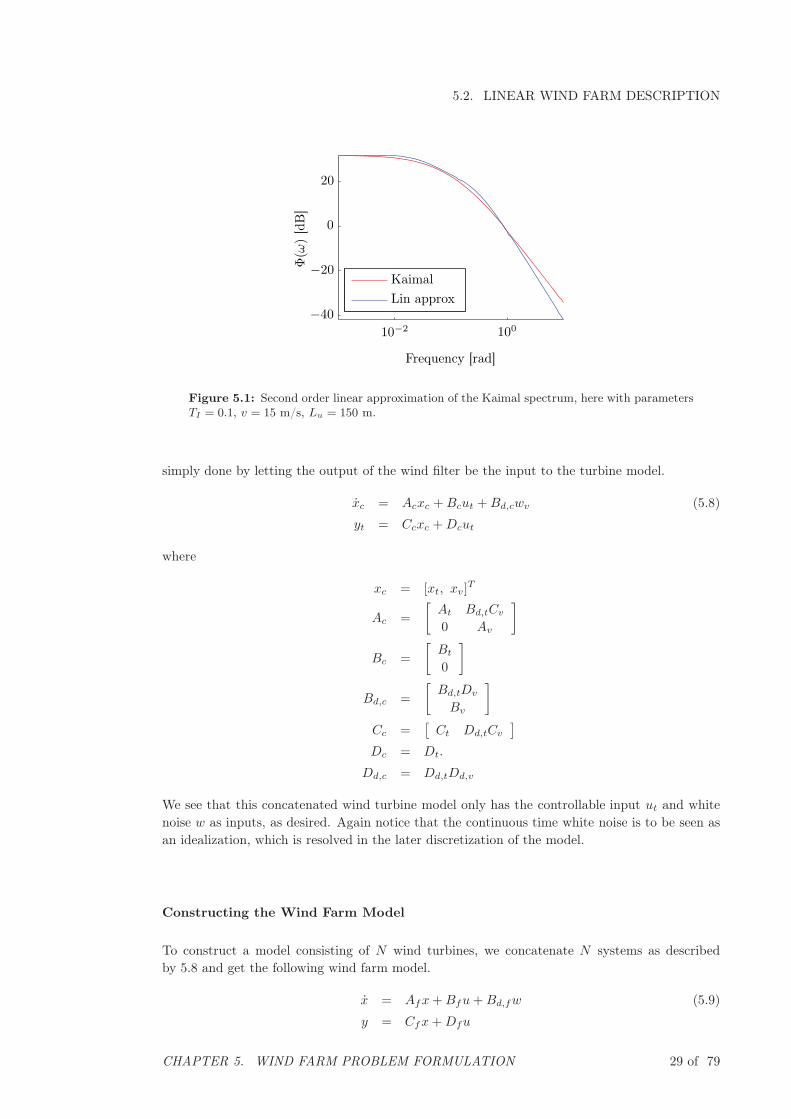
An example of the Kaimal spectrum is depicted in Figure 5.1. The spectrum is fitted manuallywith pole-zero placement with a second order linear filter G, which is depicted in the same plot.The linear model is a 2nd order model and is found in:
matlab/wind_filter/wind_filter.m
Hereby we have a linear model of the wind field dynamics by Equation 5.6.
5.2.3 Linear Wind Farm Model
We construct the wind farm model with N turbines in three steps. First we incorporate the windmodel into the wind turbine model. Secondly we concatenate N of these turbine models to obtaina model of an entire wind farm. Finally we perform a discretization of the wind farm model.
Combining the Wind Turbine and Wind Field Model
We can now concatenate the model of the wind field, with the model of the wind turbine. Herebywe obtain a model of the wind turbine, taking only white noise as uncontrollable input. This is
28 of 79 CHAPTER 5. WIND FARM PROBLEM FORMULATION
5.2. LINEAR WIND FARM DESCRIPTION
Lin approx
Kaimal
Φ(ω
)[d
B]
Frequency [rad]
10−2 100−40
−20
0
20
Figure 5.1: Second order linear approximation of the Kaimal spectrum, here with parametersTI = 0.1, v = 15 m/s, Lu = 150 m.
simply done by letting the output of the wind filter be the input to the turbine model.
xc = Acxc +Bcut +Bd,cwv (5.8)
yt = Ccxc +Dcut
where
xc = [xt, xv]T
Ac =
[At Bd,tCv
0 Av
]
Bc =
[Bt
0
]
Bd,c =
[Bd,tDv
Bv
]
Cc =[Ct Dd,tCv
]Dc = Dt.
Dd,c = Dd,tDd,v
We see that this concatenated wind turbine model only has the controllable input ut and whitenoise w as inputs, as desired. Again notice that the continuous time white noise is to be seen asan idealization, which is resolved in the later discretization of the model.
Constructing the Wind Farm Model
To construct a model consisting of N wind turbines, we concatenate N systems as describedby 5.8 and get the following wind farm model.
x = Afx+Bfu+Bd,fw (5.9)
y = Cfx+Dfu
CHAPTER 5. WIND FARM PROBLEM FORMULATION 29 of 79

5.3. QUADRATIC FATIGUE DESCRIPTION
where the system simply is obtained by block concatenation
Af = diag(Ac, . . . , Ac)
Bf = diag(Bc, . . . , Bc)
Bd,f = diag(Bd,c, . . . , Bd,c)
Cf = diag(Cc, . . . , Cc)
Df = diag(Dc, . . . , Dc)
x = [xTc,1, . . . , x
Tc,N ]T
y = [yTt,1, . . . , yTt,N ]T
w = [wv,1, . . . , wv,N ]T .
Each of the new wind farm model matrices contain N turbine model matrices. In this formulationall N turbine models are assumed identical. Inserting different turbine models can however readilybe done.
Discrete Wind Farm Model
We are now ready to present the final wind turbine model, based on the above. The last step isto discretize the continuous wind turbine model described by Equations 5.9. This is done by zeroorder hold with a given sample time Ts. The wind farm model thus becomes
x(k + 1) = Ax(k) +Bu(k) +Bdw(k) (5.10)
y(k) = Cx(k) +Du(k).
We now have a discrete linear representation of a wind farm consisting of N wind turbines. Eachturbine has p states, so A ∈ RNp×Np, B, Bd ∈ RNp×N , C ∈ RN×Np, D ∈ Rp×p.
The uncontrollable input due to wind w(k) is characterized by the covariance matrix W =
E(wwT ).
5.2.4 Evaluation of Linearized Model
It is desired to evaluate the performance of the linearized model. We do this by observing thebehavior of a single NREL wind turbine.
The performance evaluation is performed by comparing a linearized NREL wind turbine modelto the original NREL wind turbine model. This evaluation is conducted by applying a wind fieldsimilar to the one depicted in Figure 4.3 together with a power demand of 4 MW to both models.The linear model is linearized around the power demand operating point 4 MW and the windspeed operating point corresponding to the applied wind field, which is 20 m/s.
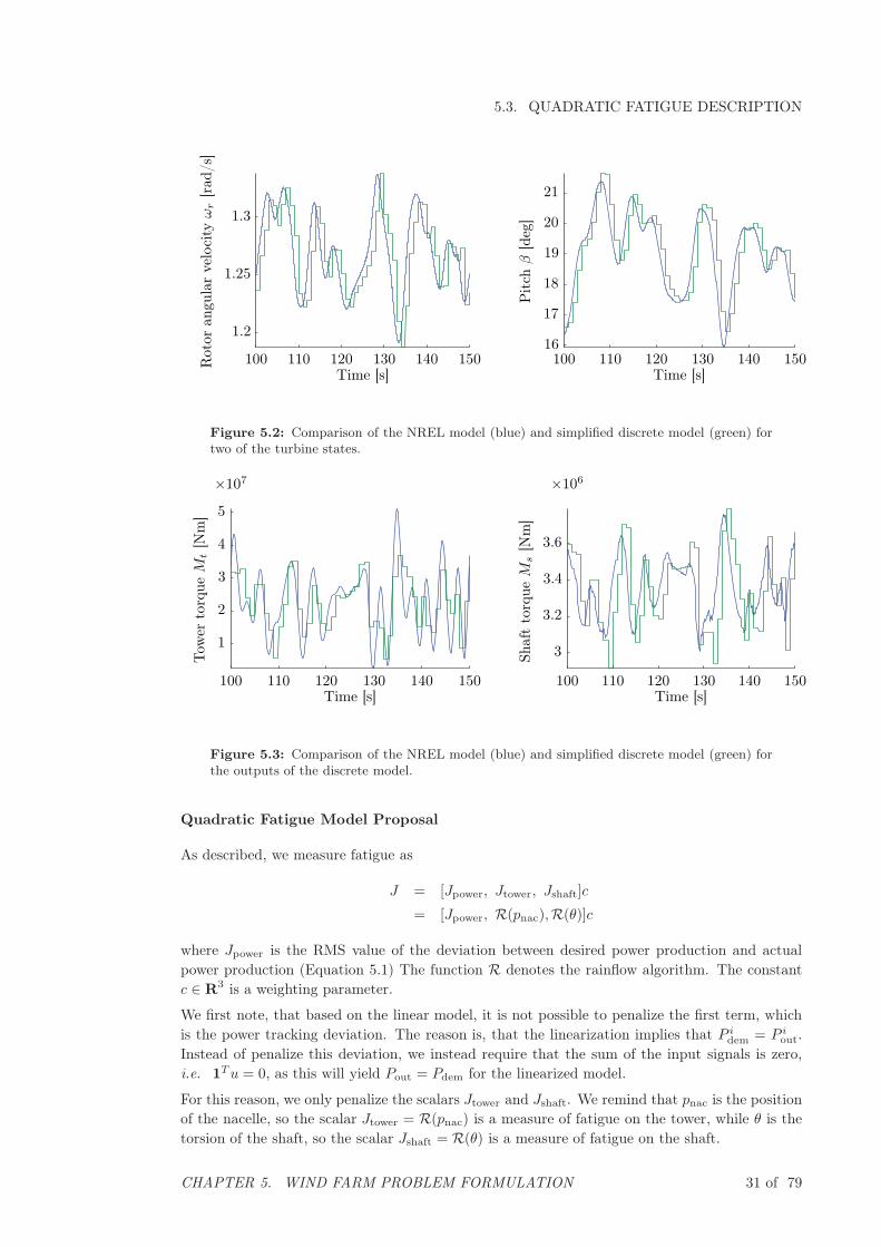
Figures 5.2 and 5.3 show four responses of the nonlinear and the discretized linear model. In thisexample a sample time of Ts = 1 is used. The figure illustrates that the linear model capturesthe dynamics of the nonlinear wind turbine model with sampling times as slow as 1 Hz.
5.3 Quadratic Fatigue Description
For controller design purpose, it is desired to have a quadratic cost function of the linearizedturbine model. This is the subject of this section, where a measure of fatigue used in the literatureis compared to the measure of fatigue base on the rainflow counting algorithm.
30 of 79 CHAPTER 5. WIND FARM PROBLEM FORMULATION
5.3. QUADRATIC FATIGUE DESCRIPTION
Rot
oran
gula
rve
loci
tyωr
[rad
/s]
Time [s]100 110 120 130 140 150
1.2
1.25
1.3
Pitch
β[d
eg]
Time [s]100 110 120 130 140 150
16
17
18
19
20
21
Figure 5.2: Comparison of the NREL model (blue) and simplified discrete model (green) fortwo of the turbine states.
Tow
erto
rque
Mt
[Nm
]
Time [s]100 110 120 130 140 150
×107
1
2
3
4
5Sh
aft
torq
ueM
s[N
m]
Time [s]100 110 120 130 140 150
×106
3
3.2
3.4
3.6
Figure 5.3: Comparison of the NREL model (blue) and simplified discrete model (green) forthe outputs of the discrete model.
Quadratic Fatigue Model Proposal
As described, we measure fatigue as
J = [Jpower, Jtower, Jshaft]c
= [Jpower, R(pnac),R(θ)]c
where Jpower is the RMS value of the deviation between desired power production and actualpower production (Equation 5.1) The function R denotes the rainflow algorithm. The constantc ∈ R3 is a weighting parameter.
We first note, that based on the linear model, it is not possible to penalize the first term, whichis the power tracking deviation. The reason is, that the linearization implies that P i
dem = P iout.
Instead of penalize this deviation, we instead require that the sum of the input signals is zero,i.e. 1Tu = 0, as this will yield Pout = Pdem for the linearized model.
For this reason, we only penalize the scalars Jtower and Jshaft. We remind that pnac is the positionof the nacelle, so the scalar Jtower = R(pnac) is a measure of fatigue on the tower, while θ is thetorsion of the shaft, so the scalar Jshaft = R(θ) is a measure of fatigue on the shaft.
CHAPTER 5. WIND FARM PROBLEM FORMULATION 31 of 79

5.3. QUADRATIC FATIGUE DESCRIPTION
The rainflow algorithm is presented in Section 4.4.2, while the parameters to be used in therainflow algorithm are presented in [Cou08]. Note that different parameters are used for thefatigue on the tower and fatigue on the shaft, such that
Bshaft = 8
Btower = 4
, see Equation 4.4.
As it is desired to have a quadratic measure of fatigue, we need an alternative to the measurebased on the rainflow algorithm. In the literature, e.g. [Spu], [MMR11] it is suggested, thatthe torque on the tower and the torque on the shaft, can be used to model fatigue on tower andshaft respectively. In the presented literature, a quadratic function of the torque on the towerQ(Mt) = |Mt|Qt
is used as a measure of fatigue on the tower, while a quadratic function on theshaft Q(Ms) = |Ms|Qs
is used as a measure of fatigue on the shaft.
This proposes that we use the following quadratic measure of fatigue
J = Q(Mt) + csQ(Ms) (5.11)
where cs ∈ R is some appropriate weight, while imposing the constraint that 1Tu = 0.
In the following, this new expression for fatigue will be evaluated based on the NREL wind turbinemodel presented in [Aeo10b].
Evaluation of Quadratic Model
In the following we will compare the proposed quadratic fatigue model Q(Ms) and Q(Mt) withthe rainflow counting based fatigue model R(θ) and R(pnac). This will be done by evaluating thecorrelation between R(pnac) and Q(Mt) and the correlation between R(θ) and Q(Ms). The goalis to verify that the quadratic model can be used as a measure of fatigue in the controller design.
The evaluation will be performed applying a control input u and wind input v to the NREL windturbine model. Based on this we measure the fatigue using both the quadratic and the rainflowmethod. Every such simulation will provide the corresponding pair (R(pnac), Q(Mt)) and thepair (R(θ), Q(Ms)). By doing this a number of time, we can observe the correlation between thetwo different fatigue measures.
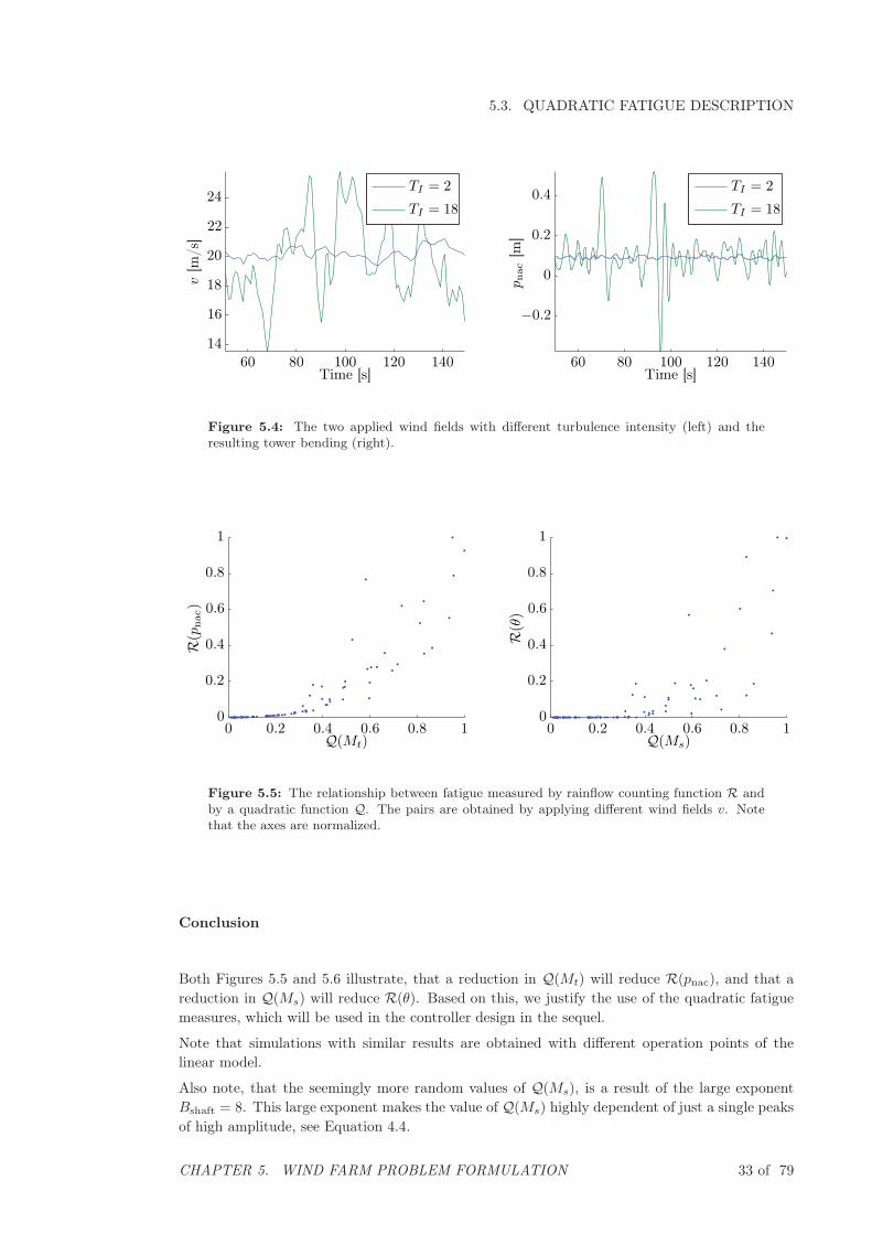
In the first evaluation, the power demand Pdem is kept constant, while wind fields of differentturbulence intensities are applied. The turbulence intensity TI is varied from 4 % to 20 %, as thiscovers the test specification in [SJBMV], which operates with turbulence intensities from 7 % to10 %.
A sample of two such wind fields is presented in Figure 5.4, along with the corresponding towerbending pnac. The tower bending obviously increases with increasing wind turbulence intensity.
The pairs (R(pnac), Q(Mt)) and (R(θ), Q(Ms)) for a number of such simulations, are illustratedin Figure 5.5.
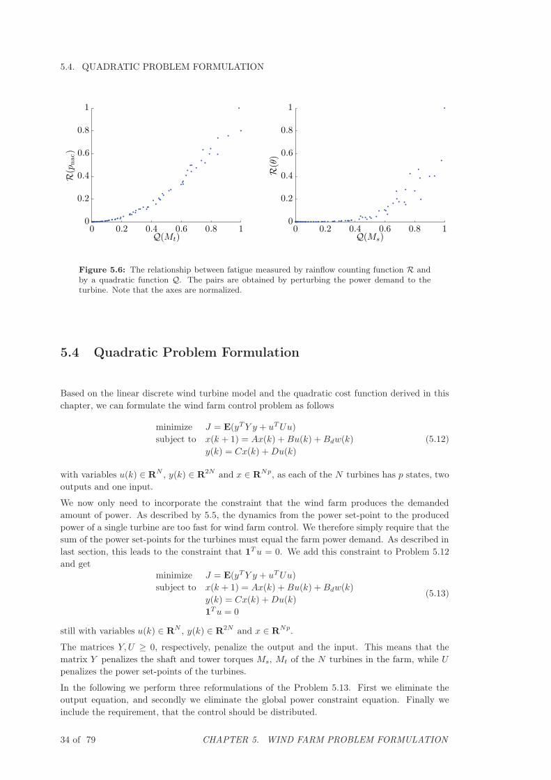
In the second evaluation, the effective wind velocity v is kept constant, while the power de-mand Pdem is perturbed with noise with different standard deviation. This results in pairs(R(pnac), Q(Mt)) and (R(θ), Q(Ms)) as illustrated in Figure 5.6.
The details of the simulations can be found in :matlab/fatigue/fatigue.m
32 of 79 CHAPTER 5. WIND FARM PROBLEM FORMULATION
5.3. QUADRATIC FATIGUE DESCRIPTION
TI = 18
TI = 2v
[m/s
]
Time [s]60 80 100 120 140
14
16
18
20
22
24TI = 18
TI = 2
pnac
[m]
Time [s]60 80 100 120 140
−0.2
0
0.2
0.4
Figure 5.4: The two applied wind fields with different turbulence intensity (left) and theresulting tower bending (right).
R(p
nac)
Q(Mt)0 0.2 0.4 0.6 0.8 1
0
0.2
0.4
0.6
0.8
1
R(θ)
Q(Ms)0 0.2 0.4 0.6 0.8 1
0
0.2
0.4
0.6
0.8
1
Figure 5.5: The relationship between fatigue measured by rainflow counting function R andby a quadratic function Q. The pairs are obtained by applying different wind fields v. Notethat the axes are normalized.
Conclusion
Both Figures 5.5 and 5.6 illustrate, that a reduction in Q(Mt) will reduce R(pnac), and that areduction in Q(Ms) will reduce R(θ). Based on this, we justify the use of the quadratic fatiguemeasures, which will be used in the controller design in the sequel.
Note that simulations with similar results are obtained with different operation points of thelinear model.
Also note, that the seemingly more random values of Q(Ms), is a result of the large exponentBshaft = 8. This large exponent makes the value of Q(Ms) highly dependent of just a single peaksof high amplitude, see Equation 4.4.
CHAPTER 5. WIND FARM PROBLEM FORMULATION 33 of 79
5.4. QUADRATIC PROBLEM FORMULATIONR(p
nac)
Q(Mt)0 0.2 0.4 0.6 0.8 1
0
0.2
0.4
0.6
0.8
1
R(θ)
Q(Ms)0 0.2 0.4 0.6 0.8 1
0
0.2
0.4
0.6
0.8
1
Figure 5.6: The relationship between fatigue measured by rainflow counting function R andby a quadratic function Q. The pairs are obtained by perturbing the power demand to theturbine. Note that the axes are normalized.
5.4 Quadratic Problem Formulation
Based on the linear discrete wind turbine model and the quadratic cost function derived in thischapter, we can formulate the wind farm control problem as follows
minimize J = E(yTY y + uTUu)
subject to x(k + 1) = Ax(k) +Bu(k) +Bdw(k)
y(k) = Cx(k) +Du(k)
(5.12)
with variables u(k) ∈ RN , y(k) ∈ R2N and x ∈ RNp, as each of the N turbines has p states, twooutputs and one input.
We now only need to incorporate the constraint that the wind farm produces the demandedamount of power. As described by 5.5, the dynamics from the power set-point to the producedpower of a single turbine are too fast for wind farm control. We therefore simply require that thesum of the power set-points for the turbines must equal the farm power demand. As described inlast section, this leads to the constraint that 1Tu = 0. We add this constraint to Problem 5.12and get
minimize J = E(yTY y + uTUu)
subject to x(k + 1) = Ax(k) +Bu(k) +Bdw(k)
y(k) = Cx(k) +Du(k)
1Tu = 0
(5.13)
still with variables u(k) ∈ RN , y(k) ∈ R2N and x ∈ RNp.
The matrices Y, U ≥ 0, respectively, penalize the output and the input. This means that thematrix Y penalizes the shaft and tower torques Ms, Mt of the N turbines in the farm, while U
penalizes the power set-points of the turbines.
In the following we perform three reformulations of the Problem 5.13. First we eliminate theoutput equation, and secondly we eliminate the global power constraint equation. Finally weinclude the requirement, that the control should be distributed.
34 of 79 CHAPTER 5. WIND FARM PROBLEM FORMULATION
5.4. QUADRATIC PROBLEM FORMULATION
Elimination of Power Output Equation
We reformulate the cost function to depend on x and u by letting
J = E(yTY y + uTUu)
= E(xTQx+ 2xTSu+ uTRu)
with Q = CTY C, S = 12 (C
TY D + CTY TD), R = DTY D + U .
Eliminating the Global Power Constraint
To eliminate the global power constraint 1Tu = 0, we find a matrix T ∈ RN×N−1 that parame-terizes the linear feasible set [BV04, p. 537]:
{u | Tu = 0} = {u | u ∈ RN−1}. (5.14)
We choose the matrix T such that [MMR11]
u1 = u1
ui = ui − ui−1, i = 1, ..., N − 1
uN = −uN−1.
which can be expressed asu = T u (5.15)
The matrix T is 1 on the main diagonal and −1 on the first lower subdiagonal. Using u asoptimization variable instead of u will guarantee that the desired power constraint 1Tu = 0 ishonored due to the transformation matrix T .
In the sequel it will become evident, that this choice of T is appropriate for the chosen formationof the wind turbines.
We change the optimization problem according to the change of variables
x(k + 1) = Ax(k) +BT u(k) +Bdw(k)
= Ax(k) + Bu(k) +Bdw(k) (5.16)
J = E(xTQx+ 2xTST u+ uTT TRT u)
= E(xTQx+ 2xT Su+ uT Ru) (5.17)
(5.18)
where we let B = BT , S = ST , R = T TRT .
It is noted, that the control signal u(k) readily is transformed to the original control signal asu = T u(k).
Distributed Feedback
Ignoring the requirement of distributed feedback, we can express the optimization problem asfollows, based on the above reformulations.
minimize J = E(xTQx+ 2xT Su+ uT Ru)
subject to x(k + 1) = Ax(k) + Bu(k) +Bdw(k)(5.19)
CHAPTER 5. WIND FARM PROBLEM FORMULATION 35 of 79

5.4. QUADRATIC PROBLEM FORMULATION
We know that the solution to a problem on this form is linear state feedback [ÅW97, p. 412]
u(k) = −Lx(k) (5.20)
with some given feedback matrix L. In terms of the original problem, the control law simplybecomes
u(k) = −Lx(k) (5.21)
where L = T L.
The requirement, that the feedback must be distributed, can be expressed by imposing a structureof the feedback matrix L. We can describe this as L ∈ L, where L ensures that the structure ofL corresponds to the available state knowledge. This imposes a structure on L which we expressas L ∈ L. In the following, we describe this structural requirement L.
For the Problem 5.19 including the constraint 5.20, we recall that
x = [xT1 , ..., x
TN ]T , u = [u1, ..., uN ]T
where xi ∈ Rp is the state of agent i and ui ∈ R is the control input of agent i.
We remind that a row formation of the turbines is assumed, where the turbines only are allowedto communicate with a given number of up- and downwind turbines. This means that agent i isallowed to calculate its respective control signal ui from the state feedback u = −Lx based solelyon knowledge of its own state xi and input ui, along with given states xj and input signals uj
from neighboring turbines, for some given set of j.
Based on this communication pattern, the structure imposed on L can be described as L ∈ L
with [MMR11]
L = {X |(X)i,j �= 0 only if i− l1 ≤ j ≤ i− l2 } , (5.22)
where l1 and l2 are parameters determining the structure. The above means that the controlinput ui to turbine i depends on l1 + 1 upwind turbines and l2 downwind turbines. This can berealized as ui = Lix = (T L)ix, and by observing the structure of T .
Final Problem Formulation
With the above reformulations, the problem formulation becomes as follows.
minimize J(L) = E(xTQx+ 2xT Su+ uT Ru)
subject to x(k + 1) = Ax(k) + Bu(k) +Bdw(k)
u(k) = −Lx(k)
L ∈ L
(5.23)
where the variables are L ∈ RN−1×Np, x ∈ RNp and u ∈ RN−1, and where E(wwT ) = W . Wenote that this is no longer a trivial Linear Quadratic Regulator (LQR) problem.
In the next chapter, we show how we iteratively can update the feedback matrix L, such that thecost J(L) is reduced.
36 of 79 CHAPTER 5. WIND FARM PROBLEM FORMULATION
Chapter 6
Modular Distributed Wind Farm
Controller
In this chapter we show how an adaptive distributed wind farm controller can be constructed,
iteratively lowering the cost of Problem 5.23. We first illustrate the principle of updating the
feedback matrix using the gradient descent method. Thereafter we show how the gradient is found
distributedly. Finally we show why the gradient descent method is used for controller updates, and
what the alternatives are.
6.1 Iterative State Feedback
The basis for the iterative feedback, is to update the optimization variable L based on measure-ments of the states x of the wind farm. Moreover, this is done distributed, such that only localmeasurements are used when updating the block of L associated with each agent.
6.1.1 The Gradient Descent Method
The problem of approximately solving a problem on a form as Problem 5.23 is treated in [MR09],and will be described in the following. The following is based on [MR09] and [MMR11].
The basis of the method, is the gradient descent method. The reason for choosing this algorithmas a basis for the distributed controller, is described in Section 6.4.
We first present the gradient descent method [BV04, p. 466].repeat
1. Set the descent direction equal to the negative gradientΔL := −∇LJ(L)
2. Choose a step length α by exact or inexact line search
3. Update the feedback matrixL := L+ αΔL
until some stopping criterion.
This algorithm must run distributed, such that each agent updates the block of the feedbackmatrix L corresponding to that agent. In the following it will be shown how this can be done by
37 of 79

6.2. DISTRIBUTED SYNTHESIS
modifying step 2 in the gradient descent method. As only local information is available at eachturbine, neither exact nor inexact line search is an option. Therefore step 2 in gradient descentmethod is omitted, and a suitable static value of α is used.
This leaves out the problem of finding ∇LJ distributed, which is the subject of the followingsection.
6.2 Distributed Synthesis
In this section, we show how the gradient of Problem 5.23 can be found by solving a set ofLyapunov equations based on the wind farm dynamics. Hereafter we show how this can be donein a distributed manner based on the adjoint system.
6.2.1 Centralized Cost Function Gradient
We observe Problem 5.23. Ignoring the structural constraint on the feedback matrix L, theproblem is given by
minimize J(L) = E(xTQx+ 2xT Su+ uT Ru)
subject to x(k + 1) = Ax(k) + Bu(k) +Bdw(k)
u(k) = −Lx(k).
(6.1)
For the function J(L) in Problem 6.1, [MMR11] shows that the gradient is given by
∇LJ = 2[RL− ST − BTP (A− BL)
]X (6.2)
where P and X are the solutions to the Lyapunov equations
X = ALXATL+W (6.3)
P = ATLPAL +QL (6.4)
with the matrices AL and QL given by
AL = A− BL (6.5)
QL = Q− SL− (SL)T + LT RL (6.6)
and where W = E(wwT ).
In the following, an argument for Equation 6.2 will be presented. We will do this by rewritingthe expression of the cost J(L), and taking the derivative.
38 of 79 CHAPTER 6. MODULAR DISTRIBUTED WIND FARM CONTROLLER

6.2. DISTRIBUTED SYNTHESIS
The cost J(L) can be expressed as
J(L) = E(xTQx+ 2xT Su+ uT Ru)
= Tr(E(xTQx+ 2xT Su+ uT Ru))
= Tr(E(xTQx− 2xT SLx+ xT LT RLx))
= Tr(E(xxT (Q− 2SL+ LT RL)))
= Tr(X(P −ATLPAL))
= Tr(XP − PALXATL))
= Tr(XP − P (X −W ))
= Tr(PW ).
Here it is used, that trace is invariant under cyclic permutations. Also it is used that E(xxT ) = X .This is realized as the system in Problem 5.13 is stationary, which means that we can write
E(x(k)x(k)T ) = E(x(k + 1)x(k + 1)T )
= E[(Ax(k) + Bu(k) + w(k))(Ax(k) + Bu(k) + w(k))T
]= ALXAT
L+W
= X.
Taking the derivative of the cost function J(L) can thus be done by taking the derivative ofTr(PW ). First we differentiate the Equation 6.4
dP = AT dPA−ATdPBL−ATPBdL− dLT BTPA− LT BT dPA+ dLT BTPBL+
LT BT dPBL+ LT BTPBdL− SdL− dLT ST + dLRL+ LRdL
= ATLdPAL +M +MT
where M = dLT (RL− ST − BTPAL). We can write this as
dP = (ATL)idPAi
L+
i−1∑k=0
(ATL)k(M +MT )Ak
L, i ∈ Z+
and thus also
dP =
∞∑k=0
(ATL)k(M +MT )Ak
L
as AL is stable.
Now we can get an expression for the desired derivative of the cost
dJ = Tr(dPW )
= Tr
(∞∑k=0
(ATL)k(M +MT )Ak
LW
)
= 2Tr(dLT (RL− ST − BTPAL)X
)(6.7)
The last equation sign follows as
X =
∞∑k=0
AkLW (AT
L)k. (6.8)
CHAPTER 6. MODULAR DISTRIBUTED WIND FARM CONTROLLER 39 of 79

6.2. DISTRIBUTED SYNTHESIS
That Equation 6.8 holds can be realized, as the right hand side is a solution to the LyapunovEquation 6.3
∞∑k=0
AkLW (AT
L)k = AL
∞∑k=0
AkLW (AT
L)kAT
L+W
=
∞∑k=1
AkLW (AT
L)k +W
=∞∑k=0
AkLW (AT
L)k.
Using the rule that dZ = Tr(dXTY ) ⇒ ∇XZ = Y [MMR11], we have the end result by Equa-tion 6.7, that
∇LJ = 2[RL− ST − BTPAL]X. (6.9)
6.2.2 Distributed Cost Function Gradient
In the distributed control method, the gradient ∇LJ must be calculated using only local andneighboring state knowledge, which calls for a reformulation of Equation 6.9. This reformulationis based on the closed loop state equation
x(k + 1) = (A− BL)x(k) + w(k) (6.10)
and on introducing the adjoint state equation with the adjoint states λ defined by
λ(k − 1) = (A− BL)Tλ(k)− (Q− SL− (SL)T + LT RL)x(k). (6.11)
By realizing that
E x(k)x(k)T = X (6.12)
Eλ(k)x(k)T = −P (A− BL)X, (6.13)
we can reformulate Equation 6.9 into [MMR11], [MR09]
∇LJ = 2((RL− ST )ExxT + BEλxT ). (6.14)
This reformulation is desired, as it enables us to find the gradient locally. The key is that bylocal and neighboring measurements of x and simulations of λ, it is possible to locally estimatethe blocks of E x(k)x(k)T and Eλ(k)x(k)T relevant to the given agent. With these estimates, itis by 6.14 possible to get an estimate of the block of ∇LJ that is relevant to the given agent.
In the following we present a proof of 6.14. It is already previously showed that Equation 6.12holds. That Equation 6.13 holds can be realized by rewriting the state Equation 6.10 as
x(k) = AiLx(k − i) +
i∑l=1
Al−1
Lw(k − l), i ∈ Z+. (6.15)
40 of 79 CHAPTER 6. MODULAR DISTRIBUTED WIND FARM CONTROLLER

6.2. DISTRIBUTED SYNTHESIS
Similarly, we can rewrite Equation 6.11 as
λ(k) = ATLλ(k + 1)−QLx(k + 1)
= (ATL)iλ(k + i)−
i−1∑j=0
(ATL)jQLx(k + 1 + j), i ∈ Z+
= −
∞∑j=0
(ATL)jQLx(k + 1 + j)
= −
∞∑j=0
(ATL)jQL
(Aj+1
Lx(k) +
j+1∑l=1
Al−1
Lw(k − l + 1 + j)
). (6.16)
The last equality sign holds as
x(k + 1 + j) = A1+j
Lx(k) +
1+j∑l=1
Al−1
Lw(k + 1 + j − l) (6.17)
by Equation 6.15.
Taking the expected value of λ(k)x(k)T using the expression for λ(k) presented in Equation 6.16yields
Eλ(k)x(k)T = E
⎛⎝−
∞∑j=0
(ATL)jQL
(Aj+1
Lx(k) +
j+1∑l=1
Al−1
Lw(k − l + 1 + j)
)x(k)T
⎞⎠
= −PALX
which is the basis of 6.14. Here it is used, that the white noise w is uncorrelated with the statex. Further it is used, that
∞∑j=0
(ATL)jQLA
j
L= P (6.18)
which follows from 6.4 as P is stable.
Motivation for the Adjoint System
In the following, we will present a short motivation for finding the adjoint system 6.11, by exam-ining the original minimization problem, and introducing the dual variable.
The optimal value of the original problem, Problem 5.13, is given by J� = J(L�). By neglectingthe noise, we can reformulate the problem as
minimize J(x, u) = xTQx+ 2xT Su+ uT Ru
subject to x(k + 1) = Ax(k) + Bu(k)(6.19)
with variables x and u. If we take the Lagrangian associated with Problem 6.19, we get [MR10]
Λ(x, u, λ) = xTQx+ 2xT Su+ uT Ru+ 2λT (x(k + 1)−Ax(k) + Bu(k)). (6.20)
Based on this, we can find the Lagrange dual function, as the minimum value of the LagrangianΛ over x, u [BV04, p. 216]. Since Λ(x, u, λ) is a convex quadratic function of x, u, we can find
CHAPTER 6. MODULAR DISTRIBUTED WIND FARM CONTROLLER 41 of 79
6.2. DISTRIBUTED SYNTHESIS
the minimizing x, u by [BV04, p. 219], [MR10]
0 = ∇xΛ(x, u, λ) = 2(Qx(k) + Su(k) + λ(k − 1)−ATλ(k))
0 = ∇uΛ(x, u, λ) = 2(STx(k) + Ru(k)− BTλ(k))
and by inserting u = Lx
0 = ∇xΛ(x, λ) = 2(Qx(k)− SLx(k) + λ(k − 1)−ATλ(k))
0 = ∇uΛ(x, λ) = 2(STx(k)− RLx(k)− BTλ(k)).
This allows us to write 0 = ∇xΛ(x, λ) − LT∇uΛ(x, λ) which leads to
λ(k − 1) = (A− BL)Tλ(k)− (Q− SL− (SL)T + LT RL)x(k) (6.21)
which is identical to Equation 6.11.
Another motivation is, that we know that distributed control is tightly related to the adjointsystems [Ran09], [MR10], [Boy10]. Also [GL00, p. 443] suggests a similar use of the adjointsystem, as an approach to iteratively finding the solution to a dynamic optimization problem.
6.2.3 Distributed System Simulation
Based on the above, we will show how the feedback matrix L can be updated iteratively in adistributed manner. Each agent updates the block of the feedback matrix relevant to the givenagent based on own measurements, and measurements from neighboring agents.
Two things are required for this distributed control to be possible. It must be possible to simulatethe adjoint states λ(k) locally on each agent. Also, it must be possible to calculate the gradient∇LJ as described by Equation 6.14 locally. Locally means, that it must be possible to do oneach individual agent using only own data and data obtained from neighboring agents. In thefollowing we will describe that this indeed is possible, due to the structure of the System 5.13.
Let us first consider the state x and the adjoint state λ. The state x can be measured locally andshared with upwind and downwind turbines.
The adjoint states must on the contrary be simulated in the backward direction based on themeasurements according to Equation 6.11. We therefore examine the structure of the terms ofEquation 6.11. The blocks in the term (A− BL)T have the structure such that
(A− BL)T ∈ {X |(X)i,j �= 0 only if i− l1 ≤ j ≤ i+ l2 + 1}
where (X)i,j denotes block i, j.
This means, that it is necessary for each turbine to know the adjoint state of l1 turbines upwindand l2 + 1 turbines downwind.
For the second term in Equation 6.11, we observe that the blocks are structured such that
(Q − SL− (SL)T + LT RL) ∈ {X |(X)i,j �= 0 only if i− l1 − 1 ≤ j ≤ i+ l2 + 1} .
This means, that to simulate the adjoint states, each turbine need to know the state of l1 + 1
turbines upwind and l2 + 1 turbines downwind.
The above concludes, that communication with l1 +1 turbines upwind and l2 +1 turbines down-wind, allows each turbine to know its own state and adjoint state. Next we show that each agentis able to calculate the local block of the gradient of the feedback matrix.
42 of 79 CHAPTER 6. MODULAR DISTRIBUTED WIND FARM CONTROLLER

6.3. CONTROL ALGORITHM
6.2.4 Distributed Gradient Calculation
We examine finding the gradient ∇LJ distributed, based on local knowledge of the state andadjoint state, using Equation 6.14. This is done by observing the two terms in Equation 6.14.The blocks of the first term are structured such that
(RL− ST ) ∈ {X |(X)i,j �= 0 only if i − l1 − 1 ≤ j ≤ i+ l2 + 1} .
This means that communication with l1 + 1 upwind turbines, and l2 + 1 turbines downwind isnecessary. With this communication enabled, E xxT can be estimated as
(E xxT )est =1
K
tk+K∑t=tk
x(t)x(x)T (6.22)
where K is the number of sample times between each update of the feedback matrix.
The second term in Equation 6.14 is BT , which has the structure
BT ∈ {X |(X)i,j �= 0 only if i− l1 ≤ j ≤ i+ l1 + 1} .
This means that communication with l1 +1 upwind turbines, and l2 turbines downwind is neces-sary. With this communication enabled, EλxT can be estimated as
(E xλT )est =1
K
tk+K∑t=tk
λ(t)x(x)T . (6.23)
6.3 Control Algorithm
We can now write the algorithm for the distributed controller. The basis of the algorithm is thateach turbine is able to access the states of l1 + 1 upwind turbines and l2 + 1 turbines downwind,and to access the simulated adjoint states of l1 turbines upwind and l2 + 1 turbines downwind.
The algorithm for turbine i can be written as [MMR11]
repeat
1. Measure local states and obtain states from neighbors, such that [xi−l1−1(t), . . . , xi+l2+1(t)]
is known for t = tk, . . . , tk+K .
2. Simulate adjoint states based on local and neighboring states and adjoint states, such that[λi−l1 (t), . . . , λi+l1+1(t)] is known for t = tk, . . . , tk+K , based on Equation 6.11.
3. Estimate the correlation of the states, and the correlation of the states and the adjointstates, based on K + 1 measured and simulated states, using Equations 6.22 and 6.23.
4. Estimate the block of the gradient corresponding to the turbine based on the correlationestimations using Equation 6.14.
5. Update the block of the gradient corresponding to the turbine by letting Li,j := Li,j +
α∇LJi,j , using a static step size α.
6. Let k = k +K.
CHAPTER 6. MODULAR DISTRIBUTED WIND FARM CONTROLLER 43 of 79

6.4. ALTERNATIVE ALGORITHMS
6.4 Alternative Algorithms
In this section, a number of alternative optimization algorithms will be described with focus onthe possibility of using them in distributed control. This will also reveal, why the gradient descentmethod is chosen above.
The reason that it is desired to find an alternative method, is to avoid the use of a static valueof α, and to increase performance.
The three alternative algorithms that are considered in the following, all seek to exploit secondorder properties of the optimization problem, in contrast to the gradient descent only using firstorder properties. Therefore we perform a second order Taylor approximation J of J at L
J(L+ v) = J(L) +∇J(L)T v +1
2vT∇2J(L)v. (6.24)
With this second order model, we capture more of the properties of the function J , that the firstorder model used in the gradient descent method. It is therefore expected that these methodswill increase the performance of the algorithm.
6.4.1 Newton’s Method
In Newton’s method, it is used that J(L + v) is a quadratic convex function in v. We can findthe minimum over v as
∂
∂vJ(L+ v) = ∇J(L) +∇2J(L)v = 0 (6.25)
which givesv = −∇2J(L)−1∇J(L). (6.26)
This is the background for Newton’s algorithm, which is [BV04, p. 487]
repeat
1. ΔL := −∇2J(L)−1∇J(L)
2. L := L+ΔL
until some stopping criterion.
A benefit of this method, is that a step size does not have to be chosen. We can therefore avoidthe use of a static α, as desired.
The method requires that the Hessian ∇2J(L) can be found distributedly. In [GL00, p. 443] it issuggested, that the Hessian also can be found by examination of the adjoint equation. But evenif the Hessian can be found in a distributed manner, the inversion of the Hessian would destroythe sparsity structure of the matrix, and make distribution of the algorithm impossible.
The use of Newton’s method in the distributed controller is therefore not examined further.
6.4.2 Conjugate Direction Method Using the Hessian
The conjugate direction method is based on the minimization of a quadratic function f(x) =
xTQx+ bTx, Q ≥ 0. We use the quadratic approximation J of J as described in Equation 6.24,and associate Q with ∇2J(L).
One form of the conjugate direction method algorithm is as follows [Lue84, p. 252].
44 of 79 CHAPTER 6. MODULAR DISTRIBUTED WIND FARM CONTROLLER

6.4. ALTERNATIVE ALGORITHMS
given some L0 initialize with g0 := ∇J(L0)T and d0 := −g0.
for k = 1 . . .N
1. Find the step length asαk := −gTk dk/d
Tk∇
2J(Lk)dk.
2. Update the solution in the direction dkLk+1 := Lk + αkdk.
3. Evaluate the gradientgk+1 := ∇J(Lk+1)
T .
4. Find a new conjugate descent directionβk := gTk+1∇
2J(Lk)gk+1/dTk∇
2J(Lk)dkdk+1 := −gk+1 + βdk.
The basis of the conjugate algorithm is as follows. Instead of always seeking for the solutionin the negative descent direction gk = −∇J(Lk)
T , as in the gradient descent method, it seeksalong a direction dk, where this direction is dependent on all previous search directions di, i < k.The method assures, that the search direction dk is conjugate to all previous search directions.With conjugate search direction we mean, that for the original minimization problem f(x) =
xTQx+ bTx it holds thatdTk Qdi = 0, for i < k. (6.27)
Hereby searching along directions we have already previously searched along is avoided. In con-trast to the gradient descent method, the minimization of a quadratic function will be independentof the condition number of the matrix. In the gradient descent method, the path of descent isoften a zig-zag movement, indicating that we essentially searched in the same directions againand again. This is avoided in the gradient descent method, as the algorithm insists that the newdirection is conjugate to the previous directions. In the pure quadratic case, we are guaranteedto find the optimum in maximum n steps, where n is the dimension of the matrix Q [Lue84, p.244].
The reason that β is chosen as described in the algorithm, is that in the quadratic case, this choicemakes the method a conjugate direction method. The motivation for choosing α as described, isthat this choice minimizes the quadratic approximation of the problem in each step [Lue84, p.245].
In contrast to Newton’s method, it is not needed to invert the Hessian, destroying the sparsitypattern. It is however seen, that in order to determine α and β, full knowledge of the directiond and the gradient g is needed. This renders this method unsuited for distributed control.
6.4.3 Conjugate Gradient Method Using Fletcher-Reeves Method
The conjugate gradient method described above can be rewritten, such that we avoid the directuse of the Hessian to represent Q [Lue84, p. 253]. Again, the method is based on the quadraticminimization problem on the form f(x) = xTQx+ bTx, Q ≥ 0.
This rewritten version of the conjugate gradient method differs from the previous algorithm in twoways. The first is, that instead of calculating the α that minimizes the quadratic approximationof the problem, a line search is performed in the conjugate direction d on the original functionJ . This line search might be exact or inexact, e.g. a backtracking line search. In this way, thismethod resembles the damped Newton’s method.
CHAPTER 6. MODULAR DISTRIBUTED WIND FARM CONTROLLER 45 of 79

6.4. ALTERNATIVE ALGORITHMS
The second change, is that the Fletcher-Reeves method is used for determination of β, assuringthat the method is a conjugate gradient method. In the quadratic case, this yields the same valueof β, as the previous method, and thus is a conjugate gradient method.
Below, the algorithm is presented [Lue84, p. 253].
given some L0 initialize with g0 := ∇J(L0)T and d0 := −g0.
for k = 1 . . .N
1. Find the step length by exact line searchαk := argminαk
J(Lk + αkdk)
or use an inexact line search algorithm.
2. Update the solution in the direction dkLk+1 := Lk + αkdk.
3. Evaluate the gradientgk+1 := ∇J(Lk+1)
T .
4. Find a new conjugate descent direction using Fletcher-Reeves methodβk := gTk+1g
Tk+1/g
Tk g
Tk
dk+1 := −gk+1 + βdk.
It is possible to implement this method distributedly, by making a few changes. As in the gradientdescent method, the choice of the step length α can not be done in a distributed manner, as thisrequires knowledge of the whole system. We therefore as in the gradient descent method, haveto use a static value of α.
The calculation of β requires full knowledge of the gradient g, in order to make the searchdirections di conjugate. This full knowledge is not available. This means that we can not requirethe full search directions di to be conjugated to each other. However, we can insist that for eachagent, the local search direction is conjugate to the previous search directions. This idea will beexplained in the following.
The variable is the feedback matrix L ∈ RN−1×Np. The descent directions di will thus have thesame structure
di =
⎡⎢⎣
d1i...
dN−1i
⎤⎥⎦ (6.28)
with dki ∈ R1×Np. The original conjugate gradient method, would require the entire searchdirection di to be conjugate to the previous search directions dj , j < i. In the distributed controlwe modify this requirement so that the conjugate direction requirement is on the basis of eachagent. This means that d1i is conjugated to d1j , j < i that d2i is conjugated to d2j , j < i etc.
The interpretation is, that each local search direction is approximately conjugate to the previouslocal search directions.
6.4.4 Choice of Optimization Algorithm
Based on the above, one candidate is found as an alternative to the gradient descent method,namely the conjugate gradient method using the Fletcher-Reeves method. This method does notresolve the problem of finding an appropriate value of the step size α. But the hope is that thissearching algorithm will converge faster, due to the fact that the method insists on making eachagent’s search direction conjugate on each other.
46 of 79 CHAPTER 6. MODULAR DISTRIBUTED WIND FARM CONTROLLER
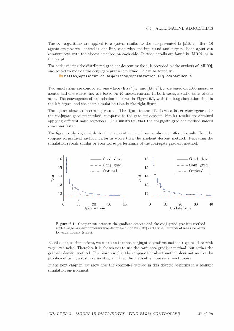
6.4. ALTERNATIVE ALGORITHMS
The two algorithms are applied to a system similar to the one presented in [MR09]. Here 10agents are present, located in one line, each with one input and one output. Each agent cancommunicate with the closest neighbor on each side. Further details are found in [MR09] or inthe script.
The code utilizing the distributed gradient descent method, is provided by the authors of [MR09],and edited to include the conjugate gradient method. It can be found in:
matlab/optimization_algorithms/optimization_alg_comparison.m
Two simulations are conducted, one where (E xxT )est and (E xλT )est are based on 1000 measure-ments, and one where they are based on 20 measurements. In both cases, a static value of α isused. The convergence of the solution is shown in Figure 6.1, with the long simulation time inthe left figure, and the short simulation time in the right figure.
The figures show to interesting results. The figure to the left shows a faster convergence, forthe conjugate gradient method, compared to the gradient descent. Similar results are obtainedapplying different noise sequences. This illustrates, that the conjugate gradient method indeedconverges faster.
The figure to the right, with the short simulation time however shows a different result. Here theconjugated gradient method performs worse than the gradient descent method. Repeating thesimulation reveals similar or even worse performance of the conjugate gradient method.
Optimal
Conj. grad.
Grad. desc.
Cos
t
Update time0 10 20 30 40
12
13
14
15
16
Optimal
Conj. grad.
Grad. desc.
Cos
t
Update time0 10 20 30 40
12
13
14
15
16
Figure 6.1: Comparison between the gradient descent and the conjugated gradient methodwith a large number of measurements for each update (left) and a small number of measurementsfor each update (right).
Based on these simulations, we conclude that the conjugated gradient method requires data withvery little noise. Therefore it is chosen not to use the conjugate gradient method, but rather thegradient descent method. The reason is that the conjugate gradient method does not resolve theproblem of using a static value of α, and that the method is more sensitive to noise.
In the next chapter, we show how the controller derived in this chapter performs in a realisticsimulation environment.
CHAPTER 6. MODULAR DISTRIBUTED WIND FARM CONTROLLER 47 of 79
Chapter 7
Controller Performance Evaluation
This chapter describes how the performance and functionality of the modular distributed wind
farm controller is evaluated, first on the linearized system, then on the more realistic wind farm
environment, using models of National Renewable Energy Laboratory (NREL) wind turbines.
7.1 Evaluation in Linear Wind Farm
In this section, the performance of the adaptive distributed control algorithm is evaluated on thelinearized wind farm using a quadratic cost function.
7.1.1 Convergence
We apply the algorithm described in Section 6.3 to a wind farm with N = 10 wind turbines.It is assumed that the turbines are placed in one row. Each wind turbine model is linearizedin the operating point vi = 15 m/s, P i
dem = 3 MW. A wind field generated according to thewind spectrum discussed in Section 4.3 on page 22 with a standard deviation of 1.5 is used asexogenous input. An example of this wind field is seen in Figure 7.3 (right). It is further assumed,that the total power demand to the whole wind farm, consisting of 10 turbines, is 30 MW.
Two different communication paths are used. The first is l1 = l2 = 0, where the turbines areallowed to communicate with one upwind and one downwind turbine. Secondly l1 = l2 = 1, wherethe turbines are allowed to have communication with two upwind and two downwind turbines.
Appropriate penalization of the input signals and output signals are chosen, through the Y and U
matrices, see Section 5.4. An appropriate static value of α is further chosen, so that the algorithmcan run distributedly
We evaluate the algorithm by allowing the system to sample the states 100 times, then updatethe feedback matrix L based on the measurement, and based on simulated adjoint states. Byletting the controller update the feedback matrix 250 times, the cost J depicted in Figure 7.1is obtained. The cost is evaluated as Tr(PW ), where P depends on L, as previously explained.The feedback matrix is initialized as L = 0, corresponding to no feedback.
The sample time used in the following results is 10 Hz. Similar results are obtained with samplingrates as slow as 1 Hz.
The conversion shows that both communication patterns lowers the cost J compared to having nofeedback, L = 0. It also shows, that it is beneficial to use the communication pattern l1 = l2 = 1,i.e. allowing communication with two upwind and two downwind turbines. At the same time it
48 of 79
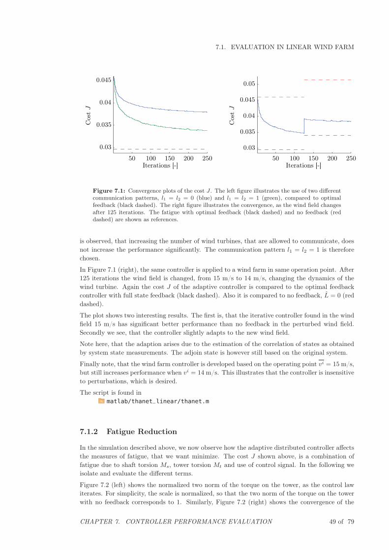
7.1. EVALUATION IN LINEAR WIND FARM
Cos
tJ
Iterations [-]50 100 150 200 250
0.03
0.035
0.04
0.045
Cos
tJ
Iterations [-]50 100 150 200 250
0.03
0.035
0.04
0.045
0.05
Figure 7.1: Convergence plots of the cost J . The left figure illustrates the use of two differentcommunication patterns, l1 = l2 = 0 (blue) and l1 = l2 = 1 (green), compared to optimalfeedback (black dashed). The right figure illustrates the convergence, as the wind field changesafter 125 iterations. The fatigue with optimal feedback (black dashed) and no feedback (reddashed) are shown as references.
is observed, that increasing the number of wind turbines, that are allowed to communicate, doesnot increase the performance significantly. The communication pattern l1 = l2 = 1 is thereforechosen.
In Figure 7.1 (right), the same controller is applied to a wind farm in same operation point. After125 iterations the wind field is changed, from 15 m/s to 14 m/s, changing the dynamics of thewind turbine. Again the cost J of the adaptive controller is compared to the optimal feedbackcontroller with full state feedback (black dashed). Also it is compared to no feedback, L = 0 (reddashed).
The plot shows two interesting results. The first is, that the iterative controller found in the windfield 15 m/s has significant better performance than no feedback in the perturbed wind field.Secondly we see, that the controller slightly adapts to the new wind field.
Note here, that the adaption arises due to the estimation of the correlation of states as obtainedby system state measurements. The adjoin state is however still based on the original system.
Finally note, that the wind farm controller is developed based on the operating point vi = 15 m/s,but still increases performance when vi = 14 m/s. This illustrates that the controller is insensitiveto perturbations, which is desired.
The script is found inmatlab/thanet_linear/thanet.m
7.1.2 Fatigue Reduction
In the simulation described above, we now observe how the adaptive distributed controller affectsthe measures of fatigue, that we want minimize. The cost J shown above, is a combination offatigue due to shaft torsion Ms, tower torsion Mt and use of control signal. In the following weisolate and evaluate the different terms.
Figure 7.2 (left) shows the normalized two norm of the torque on the tower, as the control lawiterates. For simplicity, the scale is normalized, so that the two norm of the torque on the towerwith no feedback corresponds to 1. Similarly, Figure 7.2 (right) shows the convergence of the
CHAPTER 7. CONTROLLER PERFORMANCE EVALUATION 49 of 79
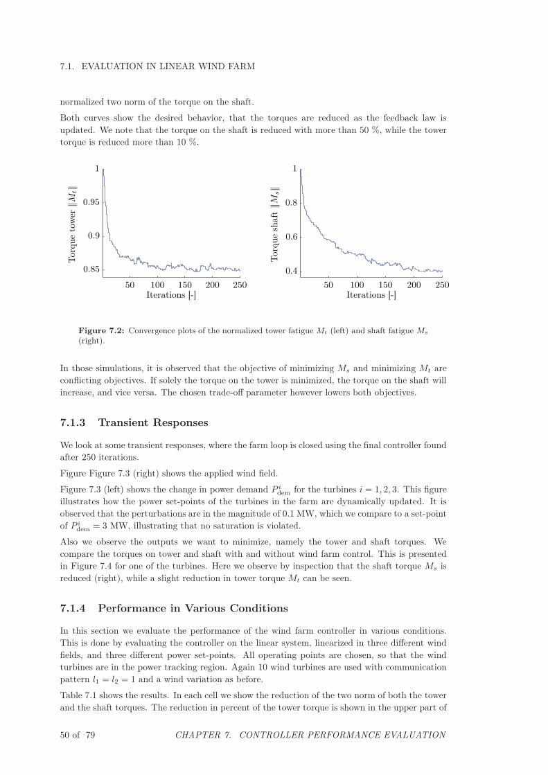
7.1. EVALUATION IN LINEAR WIND FARM
normalized two norm of the torque on the shaft.
Both curves show the desired behavior, that the torques are reduced as the feedback law isupdated. We note that the torque on the shaft is reduced with more than 50 %, while the towertorque is reduced more than 10 %.
Tor
que
tow
er‖M
t‖
Iterations [-]50 100 150 200 250
0.85
0.9
0.95
1
Tor
que
shaf
t‖M
s‖
Iterations [-]50 100 150 200 250
0.4
0.6
0.8
1
Figure 7.2: Convergence plots of the normalized tower fatigue Mt (left) and shaft fatigue Ms
(right).
In those simulations, it is observed that the objective of minimizing Ms and minimizing Mt areconflicting objectives. If solely the torque on the tower is minimized, the torque on the shaft willincrease, and vice versa. The chosen trade-off parameter however lowers both objectives.
7.1.3 Transient Responses
We look at some transient responses, where the farm loop is closed using the final controller foundafter 250 iterations.
Figure Figure 7.3 (right) shows the applied wind field.
Figure 7.3 (left) shows the change in power demand P idem for the turbines i = 1, 2, 3. This figure
illustrates how the power set-points of the turbines in the farm are dynamically updated. It isobserved that the perturbations are in the magnitude of 0.1 MW, which we compare to a set-pointof P i
dem = 3 MW, illustrating that no saturation is violated.
Also we observe the outputs we want to minimize, namely the tower and shaft torques. Wecompare the torques on tower and shaft with and without wind farm control. This is presentedin Figure 7.4 for one of the turbines. Here we observe by inspection that the shaft torque Ms isreduced (right), while a slight reduction in tower torque Mt can be seen.
7.1.4 Performance in Various Conditions
In this section we evaluate the performance of the wind farm controller in various conditions.This is done by evaluating the controller on the linear system, linearized in three different windfields, and three different power set-points. All operating points are chosen, so that the windturbines are in the power tracking region. Again 10 wind turbines are used with communicationpattern l1 = l2 = 1 and a wind variation as before.
Table 7.1 shows the results. In each cell we show the reduction of the two norm of both the towerand the shaft torques. The reduction in percent of the tower torque is shown in the upper part of
50 of 79 CHAPTER 7. CONTROLLER PERFORMANCE EVALUATION
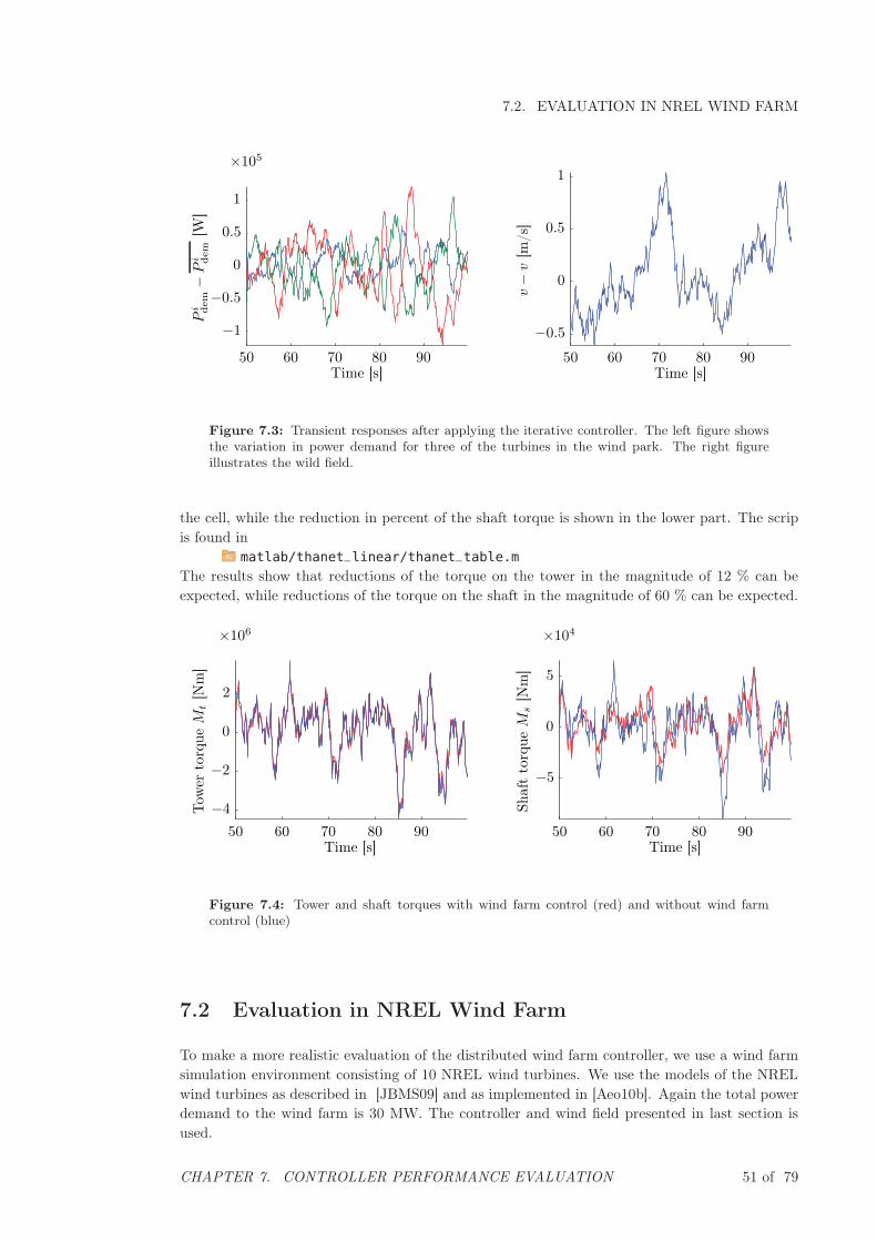
7.2. EVALUATION IN NREL WIND FARM
Pi dem−P
i dem
[W]
Time [s]50 60 70 80 90
×105
−1
−0.5
0
0.5
1
v−v
[m/s
]
Time [s]50 60 70 80 90
−0.5
0
0.5
1
Figure 7.3: Transient responses after applying the iterative controller. The left figure showsthe variation in power demand for three of the turbines in the wind park. The right figureillustrates the wild field.
the cell, while the reduction in percent of the shaft torque is shown in the lower part. The scripis found in
matlab/thanet_linear/thanet_table.m
The results show that reductions of the torque on the tower in the magnitude of 12 % can beexpected, while reductions of the torque on the shaft in the magnitude of 60 % can be expected.
Tow
erto
rque
Mt
[Nm
]
Time [s]50 60 70 80 90
×106
−4
−2
0
2
Shaf
tto
rque
Ms
[Nm
]
Time [s]50 60 70 80 90
×104
−5
0
5
Figure 7.4: Tower and shaft torques with wind farm control (red) and without wind farmcontrol (blue)
7.2 Evaluation in NREL Wind Farm
To make a more realistic evaluation of the distributed wind farm controller, we use a wind farmsimulation environment consisting of 10 NREL wind turbines. We use the models of the NRELwind turbines as described in [JBMS09] and as implemented in [Aeo10b]. Again the total powerdemand to the wind farm is 30 MW. The controller and wind field presented in last section isused.
CHAPTER 7. CONTROLLER PERFORMANCE EVALUATION 51 of 79
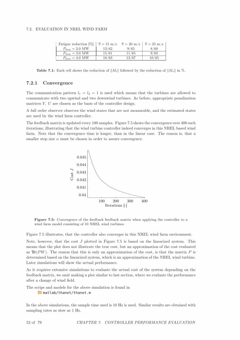
7.2. EVALUATION IN NREL WIND FARM
Fatigue reduction [%] v = 15 m/s v = 20 m/s v = 25 m/s
Pdem = 2.0 MW 13/62 9/65 8/60
Pdem = 3.0 MW 15/61 11/65 9/63
Pdem = 4.0 MW 18/63 13/67 10/65
Table 7.1: Each cell shows the reduction of ‖Mt‖ followed by the reduction of ‖Ms‖ in %.
7.2.1 Convergence
The communication pattern l1 = l2 = 1 is used which means that the turbines are allowed tocommunicate with two upwind and two downwind turbines. As before, appropriate penalizationmatrices Y, U are chosen as the basis of the controller design.
A full order observer observes the wind states that are not measurable, and the estimated statesare used by the wind farm controller.
The feedback matrix is updated every 100 samples. Figure 7.5 shows the convergence over 400 suchiterations, illustrating that the wind turbine controller indeed converges in this NREL based windfarm. Note that the convergence time is longer, than in the linear case. The reason is, that asmaller step size α must be chosen in order to assure convergence.
Cos
tJ
Iterations [-]100 200 300 400
0.04
0.041
0.042
0.043
0.044
0.045
Figure 7.5: Convergence of the feedback feedback matrix when applying the controller to awind farm model consisting of 10 NREL wind turbines.
Figure 7.5 illustrates, that the controller also converges in this NREL wind farm environment.
Note, however, that the cost J plotted in Figure 7.5 is based on the linearized system. Thismeans that the plot does not illustrate the true cost, but an approximation of the cost evaluatedas Tr(PW ). The reason that this is only an approximation of the cost, is that the matrix P isdetermined based on the linearized system, which is an approximation of the NREL wind turbine.Later simulations will show the actual performance.
As it requires extensive simulations to evaluate the actual cost of the system depending on thefeedback matrix, we omit making a plot similar to last section, where we evaluate the performanceafter a change of wind field.
The scrips and models for the above simulation is found inmatlab/thanet/thanet.m
In the above simulations, the sample time used is 10 Hz is used. Similar results are obtained withsampling rates as slow as 1 Hz.
52 of 79 CHAPTER 7. CONTROLLER PERFORMANCE EVALUATION
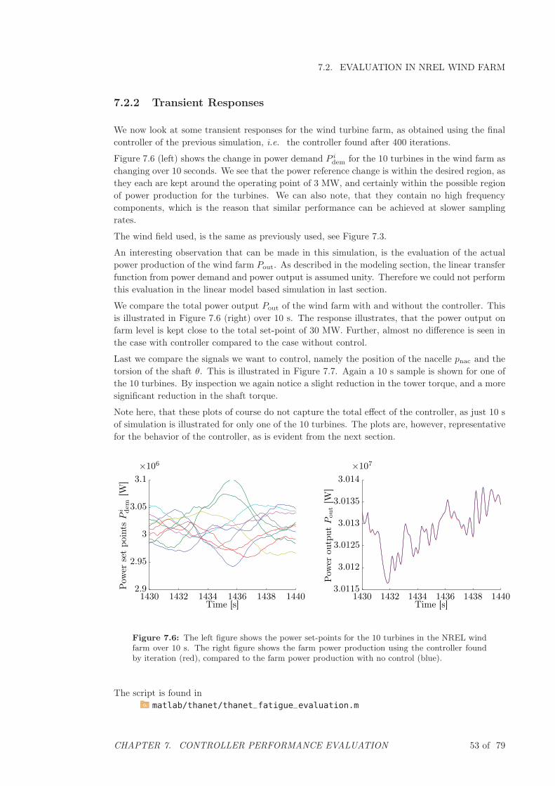
7.2. EVALUATION IN NREL WIND FARM
7.2.2 Transient Responses
We now look at some transient responses for the wind turbine farm, as obtained using the finalcontroller of the previous simulation, i.e. the controller found after 400 iterations.
Figure 7.6 (left) shows the change in power demand P idem for the 10 turbines in the wind farm as
changing over 10 seconds. We see that the power reference change is within the desired region, asthey each are kept around the operating point of 3 MW, and certainly within the possible regionof power production for the turbines. We can also note, that they contain no high frequencycomponents, which is the reason that similar performance can be achieved at slower samplingrates.
The wind field used, is the same as previously used, see Figure 7.3.
An interesting observation that can be made in this simulation, is the evaluation of the actualpower production of the wind farm Pout. As described in the modeling section, the linear transferfunction from power demand and power output is assumed unity. Therefore we could not performthis evaluation in the linear model based simulation in last section.
We compare the total power output Pout of the wind farm with and without the controller. Thisis illustrated in Figure 7.6 (right) over 10 s. The response illustrates, that the power output onfarm level is kept close to the total set-point of 30 MW. Further, almost no difference is seen inthe case with controller compared to the case without control.
Last we compare the signals we want to control, namely the position of the nacelle pnac and thetorsion of the shaft θ. This is illustrated in Figure 7.7. Again a 10 s sample is shown for one ofthe 10 turbines. By inspection we again notice a slight reduction in the tower torque, and a moresignificant reduction in the shaft torque.
Note here, that these plots of course do not capture the total effect of the controller, as just 10 sof simulation is illustrated for only one of the 10 turbines. The plots are, however, representativefor the behavior of the controller, as is evident from the next section.
Pow
erse
tpo
ints
Pi dem
[W]
Time [s]1430 1432 1434 1436 1438 1440
×106
2.9
2.95
3
3.05
3.1
Pow
erou
tput
Pout
[W]
Time [s]1430 1432 1434 1436 1438 1440
×107
3.0115
3.012
3.0125
3.013
3.0135
3.014
Figure 7.6: The left figure shows the power set-points for the 10 turbines in the NREL windfarm over 10 s. The right figure shows the farm power production using the controller foundby iteration (red), compared to the farm power production with no control (blue).
The script is found inmatlab/thanet/thanet_fatigue_evaluation.m
CHAPTER 7. CONTROLLER PERFORMANCE EVALUATION 53 of 79
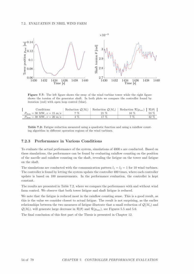
7.2. EVALUATION IN NREL WIND FARMTow
erpo
siti
onpnac
[m]
Time [s]1430 1432 1434 1436 1438 1440
0.06
0.08
0.1
0.12
0.14
Shaf
tto
rsio
nθ
[rad
]
Time [s]1430 1432 1434 1436 1438 1440
×10−3
2.7
2.8
2.9
3
Figure 7.7: The left figure shows the sway of the wind turbine tower while the right figureshows the torsion of the generator shaft. In both plots we compare the controller found byiteration (red) with open loop control (blue).
Conditions Reduction Q(Mt) Reduction Q(Ms) Reduction R(pnac) R(θ)
Pdem = 30 MW, v = 15 m/s 7 % 21 % 10 % 53 %
Pdem = 30 MW, v = 20 m/s 4 % 17 % 7 % 42 %
Table 7.2: Fatigue reduction measured using a quadratic function and using a rainflow count-ing algorithm in different operation regions of the wind turbines.
7.2.3 Performance in Various Conditions
To evaluate the actual performance of the system, simulations of 4000 s are conducted. Based onthese simulations, the performance can be found by evaluating rainflow counting on the positionof the nacelle and rainflow counting on the shaft, revealing the fatigue on the tower and fatigueon the shaft.
The simulations are conducted with the communication pattern l1 = l2 = 1 for 10 wind turbines.The controller is found by letting the system update the controller 400 times, where each controllerupdate is based on 100 measurements. In the performance evaluation, the controller is keptconstant.
The results are presented in Table 7.2, where we compare the performance with and without windfarm control. We observe that both tower fatigue and shaft fatigue is reduced.
We note that the fatigue is reduced most in the rainflow counting sense. This is a good result, asthis is the value we consider closest to actual fatigue. The result is not surprising, as the earlierrelationships between the two measures of fatigue illustrate that a small reduction of Q(Ms) andQ(Mt), will generate large decrease in R(θ) and R(pnac), see Figures 5.5 and 5.6.
The final conclusion of this first part of the Thesis is presented in Chapter 12.
54 of 79 CHAPTER 7. CONTROLLER PERFORMANCE EVALUATION

Part II
Distributed Controller for Thanet
Wind Farm
55 of 79

Chapter 8
Outline Part II
This chapter describes the outline of this second part of the Thesis. In this part of the work, a
simplified controller is developed suitable for implementation at real wind turbines. It is planned,
that this wind farm control will be evaluated in a real wind farm experiment at Thanet wind farm
in the summer of 2011.
• Thanet Wind Farm Experiment Description , Chapter 9This chapter describes possibilities and limitations for the upcoming feedback experimentsat Thanet wind farm.
• Control Strategy, Chapter 10This chapter describes how a simplified wind farm controller suitable for implementation atThanet wind farm can be designed. The goal of the controller is to illustrate the conceptof wind farm control.
• Controller Design and Evaluation, Chapter 11This final chapter describes how to design the wind farm controller, accommodating limi-tations of the wind turbines in the Thanet wind farm. Further, the controller is evaluatedon a simulation model of a wind farm.
56 of 79
Chapter 9
Thanet Wind Farm Experiment
Description
This chapter describes wind turbine experiments planned to be performed at Thanet wind farm in
the summer 2011, as a part of the Aeolus research project. Both the wind farm, the turbines in
the farm and the wind farm server are described, providing an understanding of the possibilities
and limitations of an implementation of wind farm control.
9.1 Experiment Goal
The goal of the feedback control experiment at Thanet wind farm is to illustrate than an increasein performance is achievable letting the wind turbines in the wind farm vary their power set-pointsdynamically. Demonstrating this in a real wind farm is a strong argument for further research inthis area.
9.2 Experiment Setup
The Aeolus research project has since 2009 worked with the understanding of the coupling ofwind turbines in large scale wind farms. As a primary source for development of both wind farmmodels as well as controllers, a number of experiments at the offshore wind farm Thanet are tobe performed [Ves11].
Thanet wind farm is located east of Thanet in the UK, and consists of 100 Vestas 3 MW windturbines [Ofg09], each located with a separation of 500 meters between each turbine, and 800meters between each row, see Figure 9.1.
In the Aeolus project, it is planned to evaluate a number of tests on Thanet wind farm. Theseexperiments include [Aeo11]
• Validation of single V90 turbine model.
• Validation of static and dynamic models relating effective wind speed at downwind turbineswith wind speed and the thrust coefficient of upwind turbines.
• Evaluation of static feedforward control.
• Evaluation of feedback control.
57 of 79

9.3. SYSTEM LIMITATIONS
Figure 9.1: Thanet wind farm, located 11 km off the cost of Thanet (left) [Ofg09]. The 10wind turbines selected for experiments are A01-A08 and B03-B04 (right) [Ves11].
This work treats the last item, namely feedback control.
In order to evaluate the above four tests, it has been chosen to use the 10 wind turbines A01-A08and turbines B03-B04, see figure 9.1. This choice is made such that 8 wind turbines are in arow, experiencing the wake of upwind turbines when the wind direction is along the row. Alsotwo wind turbines are located in the ambient, and thus unaffected by the wake of the 8 turbines,serving the role as a reference [Ves11].
9.3 System Limitations
The turbines in the wind farm are Vestas V90 3 MW wind turbines monitored and controlled bya Supervisory Control And Data Acquisition (SCADA) server system. The performance of thissystem, determines to what extend the experiments can be executed. The current server systemis not build with dynamic wind farm feedback control in mind, and therefore only offers limitedpossibilities options for this type of control.
In the following we present the possibilities and limitations of the SCADA server system.
Measurements of Signals
It is possible for the SCADA system controlling the wind farm to log 200 - 250 signals with afrequency of 1 Hz. It is chosen to measure the following signals during the experiments.
• Generator angular velocity
• Nacelle direction
• Pitch angle
• Power production
• Power reference
• Rotor angular velocity
• Tower acceleration longitudinal
58 of 79 CHAPTER 9. THANET WIND FARM EXPERIMENT DESCRIPTION
9.3. SYSTEM LIMITATIONS
• Tower acceleration transverse
• Wind direction
• Wind speed.
Variables
Further, the SCADA server can hold real valued variables. These variables can be updated with1 Hz based on measurements, using summation and multiplication. If x ∈ Rn are variables andy ∈ Rm are the measurements in the SCADA system, it is possible to update a variable as
x := Ax +By (9.1)
where A ∈ Rn×n and B ∈ Rn×m are constant matrices [Ves11].
Update of Power Set-Points
In the feedback control, we want to dynamically update the power set-points P idem. The SCADA
system makes it possible to update the power set-points based on multiplication and summationof measurements [Ves11]. It is assumed that also variables can be used when updating powerset-points. We can thus write the update of power set-points as
P idem := cTx+ dT y (9.2)
where c ∈ Rn and d ∈ Rm are constants.
It is desired to design the controller, such that the power set-points are updated with a frequencyof maximum 0.2 Hz. The reason is that a significant time delay is present when updating thepower set-point. Further, a significant rate on the power set-point is expected. We assume thatthe time delay is 1 second, and that the rate limit is 100 kW/s, that is∣∣∣∣P i
dem
d
dt
∣∣∣∣ ≤ 100 kW/s. (9.3)
Distributed Control
It is noticed, that all the control is implemented on the SCADA server system. This means thatthe control must be implemented in a centralized manner, not distributed.
Model of the Vestas V90 Turbine
The controller design should be based on a model of the Vestas V90 3 MW wind turbine. As thismodel is not yet available, this work will be based on the National Renewable Energy Laboratory(NREL) wind turbine model, as previously used. Designing the controller based on this windturbine will of course not give precise results, but it will be easy to change model when the VestasV90 model is available.
In the next chapter we design a controller suitable for implementation on the server system atThanet wind farm, taking the limitations present in this chapter into account.
CHAPTER 9. THANET WIND FARM EXPERIMENT DESCRIPTION 59 of 79
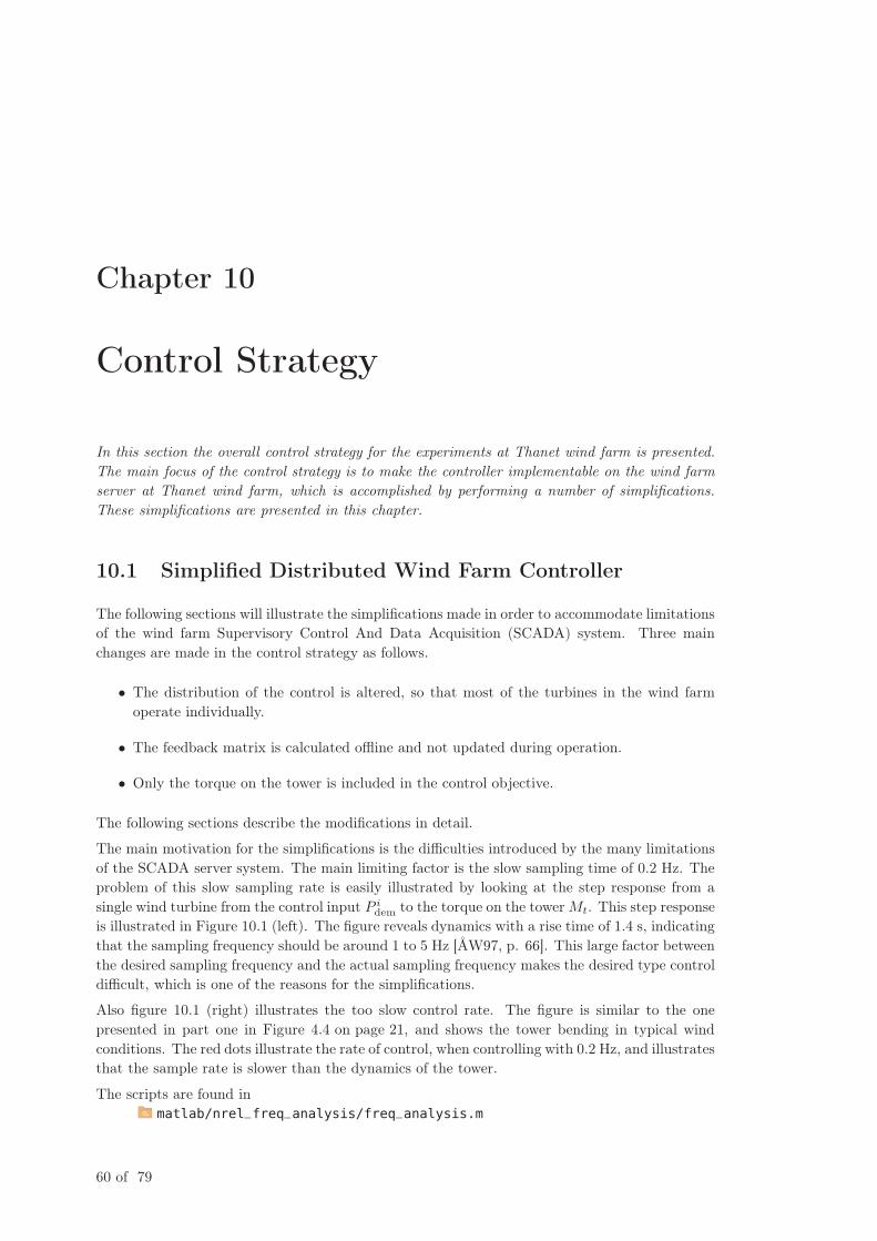
Chapter 10
Control Strategy
In this section the overall control strategy for the experiments at Thanet wind farm is presented.
The main focus of the control strategy is to make the controller implementable on the wind farm
server at Thanet wind farm, which is accomplished by performing a number of simplifications.
These simplifications are presented in this chapter.
10.1 Simplified Distributed Wind Farm Controller
The following sections will illustrate the simplifications made in order to accommodate limitationsof the wind farm Supervisory Control And Data Acquisition (SCADA) system. Three mainchanges are made in the control strategy as follows.
• The distribution of the control is altered, so that most of the turbines in the wind farmoperate individually.
• The feedback matrix is calculated offline and not updated during operation.
• Only the torque on the tower is included in the control objective.
The following sections describe the modifications in detail.
The main motivation for the simplifications is the difficulties introduced by the many limitationsof the SCADA server system. The main limiting factor is the slow sampling time of 0.2 Hz. Theproblem of this slow sampling rate is easily illustrated by looking at the step response from asingle wind turbine from the control input P i
dem to the torque on the tower Mt. This step responseis illustrated in Figure 10.1 (left). The figure reveals dynamics with a rise time of 1.4 s, indicatingthat the sampling frequency should be around 1 to 5 Hz [ÅW97, p. 66]. This large factor betweenthe desired sampling frequency and the actual sampling frequency makes the desired type controldifficult, which is one of the reasons for the simplifications.
Also figure 10.1 (right) illustrates the too slow control rate. The figure is similar to the onepresented in part one in Figure 4.4 on page 21, and shows the tower bending in typical windconditions. The red dots illustrate the rate of control, when controlling with 0.2 Hz, and illustratesthat the sample rate is slower than the dynamics of the tower.
The scripts are found inmatlab/nrel_freq_analysis/freq_analysis.m
60 of 79
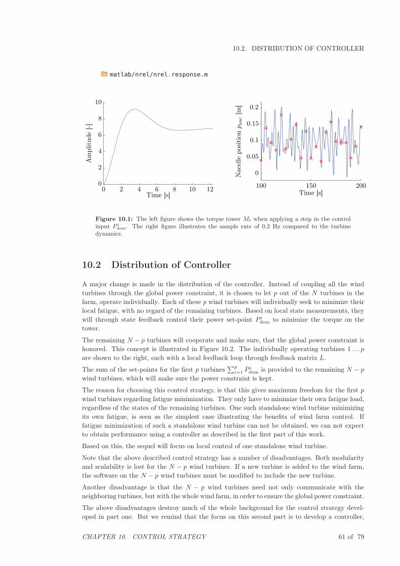
10.2. DISTRIBUTION OF CONTROLLER
matlab/nrel/nrel_response.m
Am
plit
ude
[-]
Time [s]0 2 4 6 8 10 12
0
2
4
6
8
10
Nac
elle
posi
tion
pnac
[m]
Time [s]100 150 200
0
0.05
0.1
0.15
0.2
Figure 10.1: The left figure shows the torque tower Mt when applying a step in the controlinput P i
dem. The right figure illustrates the sample rate of 0.2 Hz compared to the turbinedynamics.
10.2 Distribution of Controller
A major change is made in the distribution of the controller. Instead of coupling all the windturbines through the global power constraint, it is chosen to let p out of the N turbines in thefarm, operate individually. Each of these p wind turbines will individually seek to minimize theirlocal fatigue, with no regard of the remaining turbines. Based on local state measurements, theywill through state feedback control their power set-point P i
dem to minimize the torque on thetower.
The remaining N − p turbines will cooperate and make sure, that the global power constraint ishonored. This concept is illustrated in Figure 10.2. The individually operating turbines 1 . . . p
are shown to the right, each with a local feedback loop through feedback matrix L.
The sum of the set-points for the first p turbines∑p
i=1 Pidem is provided to the remaining N − p
wind turbines, which will make sure the power constraint is kept.
The reason for choosing this control strategy, is that this gives maximum freedom for the first p
wind turbines regarding fatigue minimization. They only have to minimize their own fatigue load,regardless of the states of the remaining turbines. One such standalone wind turbine minimizingits own fatigue, is seen as the simplest case illustrating the benefits of wind farm control. Iffatigue minimization of such a standalone wind turbine can not be obtained, we can not expectto obtain performance using a controller as described in the first part of this work.
Based on this, the sequel will focus on local control of one standalone wind turbine.
Note that the above described control strategy has a number of disadvantages. Both modularityand scalability is lost for the N − p wind turbines. If a new turbine is added to the wind farm,the software on the N − p wind turbines must be modified to include the new turbine.
Another disadvantage is that the N − p wind turbines need not only communicate with theneighboring turbines, but with the whole wind farm, in order to ensure the global power constraint.
The above disadvantages destroy much of the whole background for the control strategy devel-oped in part one. But we remind that the focus on this second part is to develop a controller,
CHAPTER 10. CONTROL STRATEGY 61 of 79
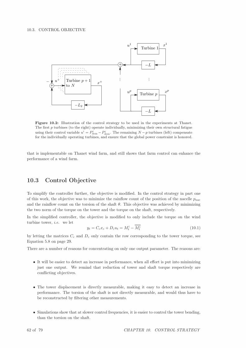
10.3. CONTROL OBJECTIVE
u1
−L
...
−L
up
−L2
...
Turbine p
Turbine 1
Turbine p+ 1to N
x1
xp
x+u+−
Figure 10.2: Illustration of the control strategy to be used in the experiments at Thanet.The first p turbines (to the right) operate individually, minimizing their own structural fatigue
using their control variable ui = P i
dem −P i
dem. The remaining N − p turbines (left) compensate
for the individually operating turbines, and ensure that the global power constraint is honored.
that is implementable on Thanet wind farm, and still shows that farm control can enhance theperformance of a wind farm.
10.3 Control Objective
To simplify the controller further, the objective is modified. In the control strategy in part oneof this work, the objective was to minimize the rainflow count of the position of the nacelle pnacand the rainflow count on the torsion of the shaft θ. This objective was achieved by minimizingthe two norm of the torque on the tower and the torque on the shaft, respectively.
In the simplified controller, the objective is modified to only include the torque on the windturbine tower, i.e. we let
yt = Ccxc +Dcut = M it −M i
t (10.1)
by letting the matrices Cc and Dc only contain the row corresponding to the tower torque, seeEquation 5.8 on page 29.
There are a number of reasons for concentrating on only one output parameter. The reasons are:
• It will be easier to detect an increase in performance, when all effort is put into minimizingjust one output. We remind that reduction of tower and shaft torque respectively areconflicting objectives.
• The tower displacement is directly measurable, making it easy to detect an increase inperformance. The torsion of the shaft is not directly measurable, and would thus have tobe reconstructed by filtering other measurements.
• Simulations show that at slower control frequencies, it is easier to control the tower bending,than the torsion on the shaft.
62 of 79 CHAPTER 10. CONTROL STRATEGY

10.4. LINEAR QUADRATIC CONTROL
10.4 Linear Quadratic Control
As mentioned above, the aspect of modularity and scalability is lost, due to the new commu-nication pattern. This means that there is no reason to update the feedback matrix online, asthis was done to achieve modularity and scalability. Moreover it is noted, the calculations andmemory necessary to update the feedback matrix exceed the limits of the SCADA system.
Therefore it is chosen to implement linear quadratic control in the wind farm, using a predeter-mined feedback matrix. A feedback controller must therefore be derived for the p individuallyoperating wind turbines, feeding back the states to the power set-point. Similarly, a feedbackmatrix must be designed for the remaining N − p cooperating turbines. This feedback matrixmust assure that the power demand is honored.
In the sequel, we will only consider the controller for the p standalone wind turbines. In the nextchapter we design this controller and evaluate the performance.
CHAPTER 10. CONTROL STRATEGY 63 of 79

Chapter 11
Controller Design and Evaluation
This chapter presents the problem formulation of tower fatigue minimization of a standalone wind
turbine. Following, a controller is designed, taking the limitations of the Supervisory Control And
Data Acquisition (SCADA) server system into account. Finally the performance is examined
through simulations.
11.1 Problem Formulation
Based on the setup described in last chapter, we develop a controller for one standalone windturbine. This corresponds to the control of one of the p wind turbines, operating alone. We donot consider the remaining N − p turbines.
In the following we present a problem formulation for fatigue minimization on a single windturbine.
After removing the shaft torque as an output, we get the system
xc(t) = Acxc(t) +Bcut(t) +Bd,cwv(t)
yt(t) = Ccxc(t),
see 5.8.
The state of this system includes the wind turbine states and the wind state. The output is thesmall signal values of the torque on the tower while the input is the small signal value of thepower set-point
xc(t) =
⎡⎢⎢⎢⎣
β(t)− β
ωr(t)− ωr
ωfiltg (t)− ωfilt
g
xv(t)− xt
⎤⎥⎥⎥⎦ yt(t) = Mt(t)−Mt ut(t) = Pdem(t)− Pdem. (11.1)
The term w is the uncontrollable noise input, due to the effect of the wind. Again we note thatthe white noise term has infinite energy, and therefore involves some idealization [GL00, p. 108].
The cost function is a trade-off between minimizing the control signal and minimizing the towertorque variation. We will formulate the cost in discrete time later in this chapter.
64 of 79
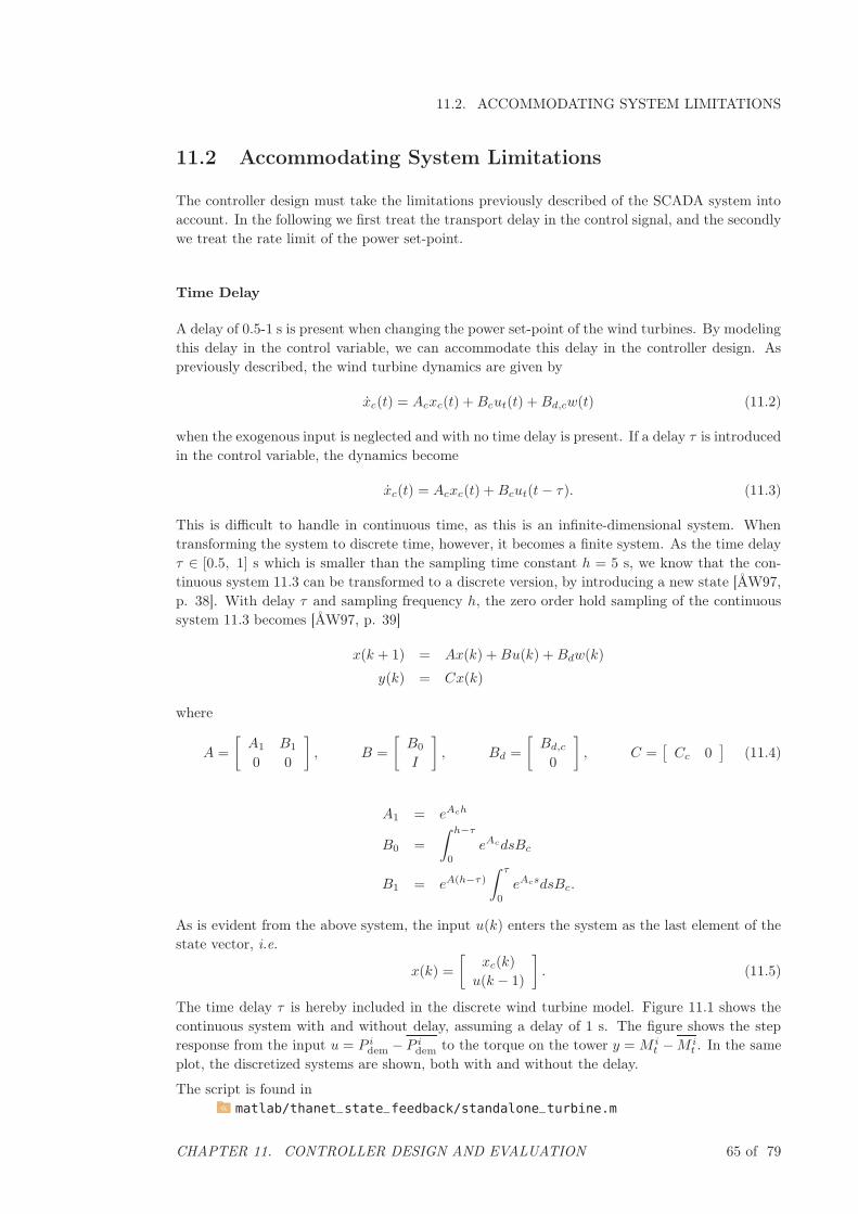
11.2. ACCOMMODATING SYSTEM LIMITATIONS
11.2 Accommodating System Limitations
The controller design must take the limitations previously described of the SCADA system intoaccount. In the following we first treat the transport delay in the control signal, and the secondlywe treat the rate limit of the power set-point.
Time Delay
A delay of 0.5-1 s is present when changing the power set-point of the wind turbines. By modelingthis delay in the control variable, we can accommodate this delay in the controller design. Aspreviously described, the wind turbine dynamics are given by
xc(t) = Acxc(t) +Bcut(t) +Bd,cw(t) (11.2)
when the exogenous input is neglected and with no time delay is present. If a delay τ is introducedin the control variable, the dynamics become
xc(t) = Acxc(t) +Bcut(t− τ). (11.3)
This is difficult to handle in continuous time, as this is an infinite-dimensional system. Whentransforming the system to discrete time, however, it becomes a finite system. As the time delayτ ∈ [0.5, 1] s which is smaller than the sampling time constant h = 5 s, we know that the con-tinuous system 11.3 can be transformed to a discrete version, by introducing a new state [ÅW97,p. 38]. With delay τ and sampling frequency h, the zero order hold sampling of the continuoussystem 11.3 becomes [ÅW97, p. 39]
x(k + 1) = Ax(k) +Bu(k) +Bdw(k)
y(k) = Cx(k)
where
A =
[A1 B1
0 0
], B =
[B0
I
], Bd =
[Bd,c
0
], C =
[Cc 0
](11.4)
A1 = eAch
B0 =
∫ h−τ
0
eAcdsBc
B1 = eA(h−τ)
∫ τ
0
eAcsdsBc.
As is evident from the above system, the input u(k) enters the system as the last element of thestate vector, i.e.
x(k) =
[xc(k)
u(k − 1)
]. (11.5)
The time delay τ is hereby included in the discrete wind turbine model. Figure 11.1 shows thecontinuous system with and without delay, assuming a delay of 1 s. The figure shows the stepresponse from the input u = P i
dem − P idem to the torque on the tower y = M i
t −M it . In the same
plot, the discretized systems are shown, both with and without the delay.
The script is found inmatlab/thanet_state_feedback/standalone_turbine.m
CHAPTER 11. CONTROLLER DESIGN AND EVALUATION 65 of 79
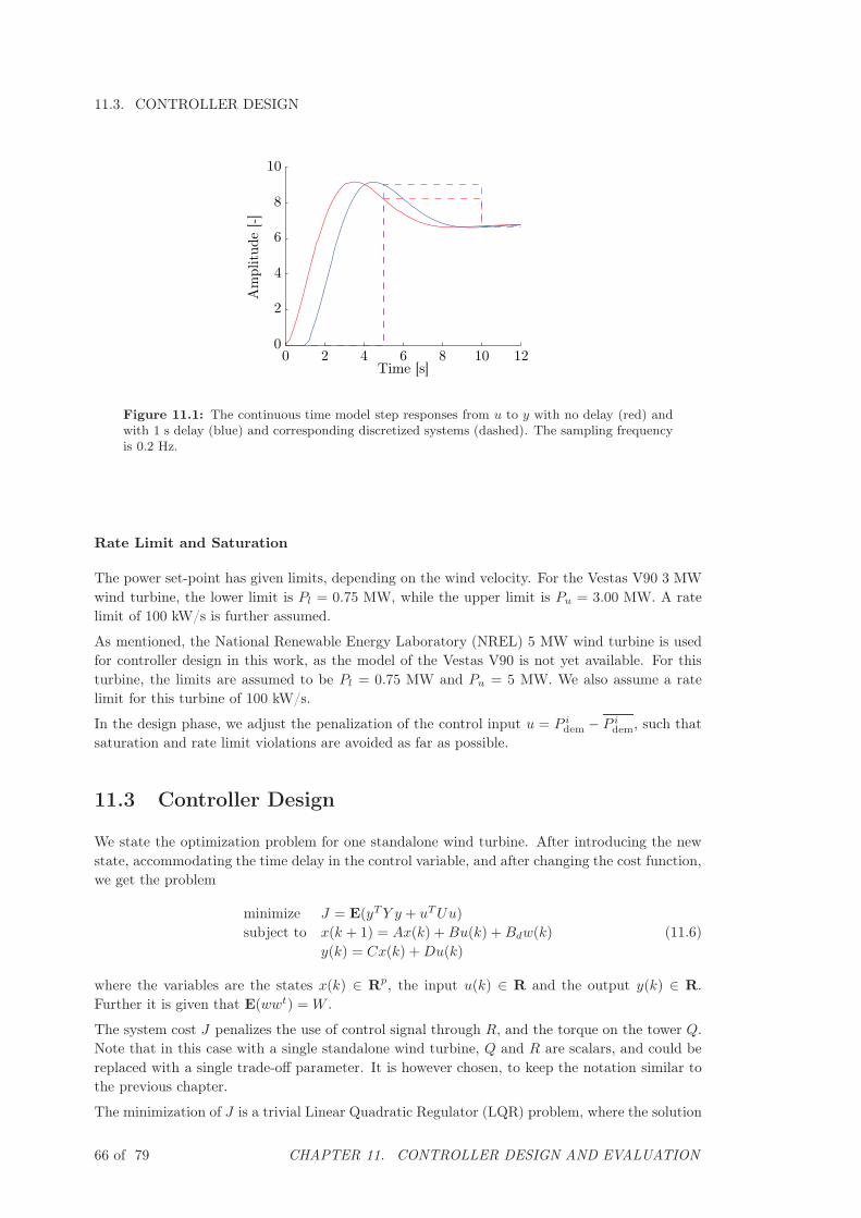
11.3. CONTROLLER DESIGN
Am
plit
ude
[-]
Time [s]0 2 4 6 8 10 12
0
2
4
6
8
10
Figure 11.1: The continuous time model step responses from u to y with no delay (red) andwith 1 s delay (blue) and corresponding discretized systems (dashed). The sampling frequencyis 0.2 Hz.
Rate Limit and Saturation
The power set-point has given limits, depending on the wind velocity. For the Vestas V90 3 MWwind turbine, the lower limit is Pl = 0.75 MW, while the upper limit is Pu = 3.00 MW. A ratelimit of 100 kW/s is further assumed.
As mentioned, the National Renewable Energy Laboratory (NREL) 5 MW wind turbine is usedfor controller design in this work, as the model of the Vestas V90 is not yet available. For thisturbine, the limits are assumed to be Pl = 0.75 MW and Pu = 5 MW. We also assume a ratelimit for this turbine of 100 kW/s.
In the design phase, we adjust the penalization of the control input u = P idem − P i
dem, such thatsaturation and rate limit violations are avoided as far as possible.
11.3 Controller Design
We state the optimization problem for one standalone wind turbine. After introducing the newstate, accommodating the time delay in the control variable, and after changing the cost function,we get the problem
minimize J = E(yTY y + uTUu)
subject to x(k + 1) = Ax(k) +Bu(k) +Bdw(k)
y(k) = Cx(k) +Du(k)
(11.6)
where the variables are the states x(k) ∈ Rp, the input u(k) ∈ R and the output y(k) ∈ R.Further it is given that E(wwt) = W .
The system cost J penalizes the use of control signal through R, and the torque on the tower Q.Note that in this case with a single standalone wind turbine, Q and R are scalars, and could bereplaced with a single trade-off parameter. It is however chosen, to keep the notation similar tothe previous chapter.
The minimization of J is a trivial Linear Quadratic Regulator (LQR) problem, where the solution
66 of 79 CHAPTER 11. CONTROLLER DESIGN AND EVALUATION
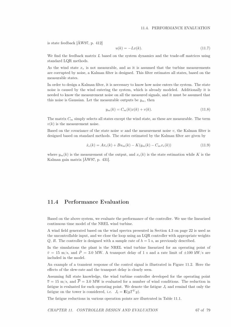
11.4. PERFORMANCE EVALUATION
is state feedback [ÅW97, p. 412]u(k) = −Lx(k). (11.7)
We find the feedback matrix L based on the system dynamics and the trade-off matrices usingstandard LQR methods.
As the wind state xv is not measurable, and as it is assumed that the turbine measurementsare corrupted by noise, a Kalman filter is designed. This filter estimates all states, based on themeasurable states.
In order to design a Kalman filter, it is necessary to know how noise enters the system. The statenoise is caused by the wind entering the system, which is already modeled. Additionally it isneeded to know the measurement noise on all the measured signals, and it must be assumed thatthis noise is Gaussian. Let the measurable outputs be ym, then
ym(k) = Cm(k)x(k) + v(k). (11.8)
The matrix Cm simply selects all states except the wind state, as these are measurable. The termv(k) is the measurement noise.
Based on the covariance of the state noise w and the measurement noise v, the Kalman filter isdesigned based on standard methods. The states estimated by the Kalman filter are given by
xe(k) = Axe(k) +Bum(k)−K(ym(k)− Cmxe(k)) (11.9)
where ym(k) is the measurement of the output, and xe(k) is the state estimation while K is theKalman gain matrix [ÅW97, p. 431].
11.4 Performance Evaluation
Based on the above system, we evaluate the performance of the controller. We use the linearizedcontinuous time model of the NREL wind turbine.
A wind field generated based on the wind spectra presented in Section 4.3 on page 22 is used asthe uncontrollable input, and we close the loop using an LQR controller with appropriate weightsQ, R. The controller is designed with a sample rate of h = 5 s, as previously described.
In the simulations the plant is the NREL wind turbine linearized for an operating point ofv = 15 m/s, and P = 3.0 MW. A transport delay of 1 s and a rate limit of ±100 kW/s areincluded in the model.
An example of a transient response of the control signal is illustrated in Figure 11.2. Here theeffects of the slew-rate and the transport delay is clearly seen.
Assuming full state knowledge, the wind turbine controller developed for the operating pointv = 15 m/s, and P = 3.0 MW is evaluated for a number of wind conditions. The reduction infatigue is evaluated for each operating point. We denote the fatigue Jt and remind that only thefatigue on the tower is considered, i.e. Jt = E(yT Y y).
The fatigue reductions in various operation points are illustrated in Table 11.1.
CHAPTER 11. CONTROLLER DESIGN AND EVALUATION 67 of 79
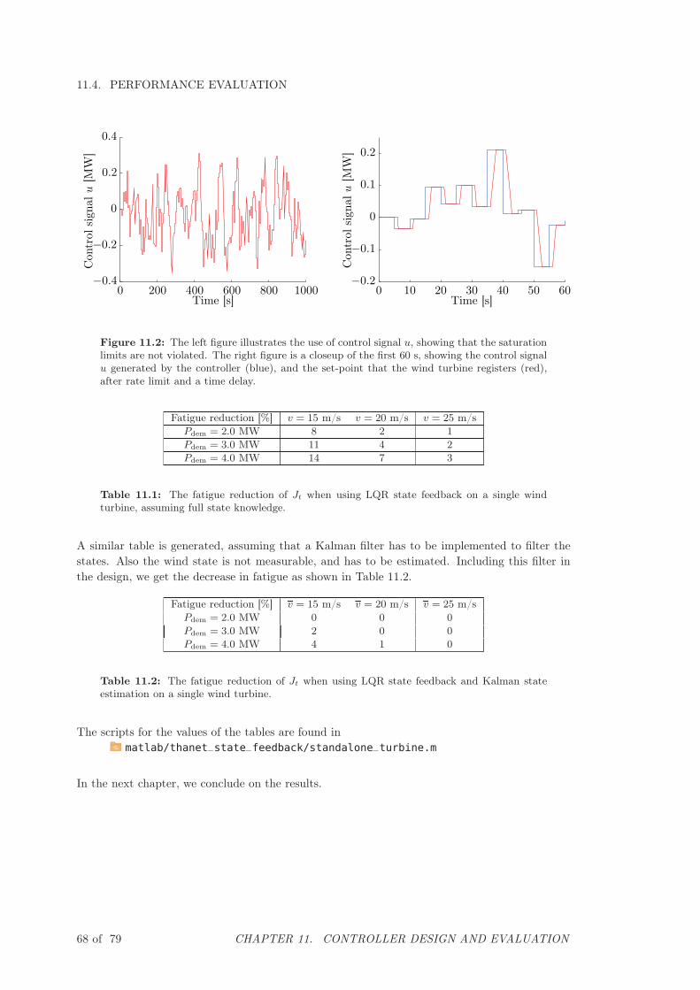
11.4. PERFORMANCE EVALUATIONC
ontr
olsi
gnal
u[M
W]
Time [s]0 200 400 600 800 1000
−0.4
−0.2
0
0.2
0.4
Con
trol
sign
alu
[MW
]
Time [s]0 10 20 30 40 50 60
−0.2
−0.1
0
0.1
0.2
Figure 11.2: The left figure illustrates the use of control signal u, showing that the saturationlimits are not violated. The right figure is a closeup of the first 60 s, showing the control signalu generated by the controller (blue), and the set-point that the wind turbine registers (red),after rate limit and a time delay.
Fatigue reduction [%] v = 15 m/s v = 20 m/s v = 25 m/s
Pdem = 2.0 MW 8 2 1
Pdem = 3.0 MW 11 4 2
Pdem = 4.0 MW 14 7 3
Table 11.1: The fatigue reduction of Jt when using LQR state feedback on a single windturbine, assuming full state knowledge.
A similar table is generated, assuming that a Kalman filter has to be implemented to filter thestates. Also the wind state is not measurable, and has to be estimated. Including this filter inthe design, we get the decrease in fatigue as shown in Table 11.2.
Fatigue reduction [%] v = 15 m/s v = 20 m/s v = 25 m/s
Pdem = 2.0 MW 0 0 0
Pdem = 3.0 MW 2 0 0
Pdem = 4.0 MW 4 1 0
Table 11.2: The fatigue reduction of Jt when using LQR state feedback and Kalman stateestimation on a single wind turbine.
The scripts for the values of the tables are found inmatlab/thanet_state_feedback/standalone_turbine.m
In the next chapter, we conclude on the results.
68 of 79 CHAPTER 11. CONTROLLER DESIGN AND EVALUATION

Part III
Epilogue
69 of 79
Chapter 12
Conclusion
In this work, we considered the control of a wind farm consisting of a large number of turbines.
The basis of this wind farm control is the freedom that lies in the power distribution among the
turbines, when there is more power available, than demanded. The focus of this work was to
distribute the power demand to the turbines in the farm dynamically, such that the total fatigue
on the turbines in the farm is minimized. At the same time the power demand to the farm must
be met. In the first part of this work we showed that this power distribution can be achieved by a
distributed controller. Moreover, we demonstrated that this controller can be designed such that
it is both modular and scalable. The second part concerned the upcoming experiments at Thanet
wind farm. In this part of the work, we developed a new controller, taking the limitations of the
wind farm server system at Thanet into account.
12.1 Modular Distributed Wind Farm Control
In the first part of the thesis, we designed a distributed modular and scalable wind farm controller.The basis of the controller was the coupling of the wind turbines through the total power demandto the wind farm. The coupling of the turbines through the wind field was neglected.
We showed that a freedom lies in the distribution of the total wind farm power demand to theindividual turbines in the wind farm. When there is an excess of wind energy available, we arefree to distribute the power demand among the wind turbines, as long as the farm power demandis met.
Based on this freedom, a controller was designed that dynamically generates set-points for theturbines in the farm, using turbine measurements. The objective of the controller was to reducethe total fatigue on the turbines in the farm, while still honoring the farm power demand. Fatigueon both turbine tower and generator shaft were taken into account.
Further we showed that the designed controller is both modular and scalable. This gives thedesired properties, that the controller on each wind turbine in the farm is identical. Also it ispossible to add or remove turbines from the wind farm, without changing the controller on theremaining turbines.
The basis of the controller is distributed state feedback. Each turbine controls its power set-point,by feeding back own and neighboring measurements. Moreover, each turbine updates the localcontrol law iteratively, based on local and neighboring measurements.
By simulations in a linear wind farm model, this iterative controller was verified. The simulationsshowed that the modular and scalable design indeed is implementable, and that the distributed
70 of 79
12.2. DISTRIBUTED CONTROLLER FOR THANET WIND FARM
controller converges. The controller was also examined in various wind fields to demonstraterobustness against changes in the wind field.
Further simulations were performed in a realistic wind farm environment consisting of 10 NRELwind turbine models. The simulations confirmed the functionality of the distributed controlstrategy. Also these simulations revealed, that fatigue reductions in the magnitude of 50 % forthe shaft and 10 % for the tower could be achieved.
Based on this we conclude that the area of wind farm control is a promising approach to fatiguereduction in wind farms. With the only requirements that the turbines are allowed to commu-nicate with neighbors and change their power set-points dynamically, we can reduce the fatigueon both the turbine tower shaft significantly. Moreover we conclude, that this controller can bedesigned as both modular and scalable such that turbines can be removed or added to the farm,without altering the software on the remaining turbines.
12.2 Distributed Controller for Thanet Wind Farm
In the second part of the thesis, we considered upcoming wind farm experiments, planned tobe performed at Thanet wind farm in the summer of 2011. The goal of the experiments is todemonstrate the concept of fatigue reduction through dynamic power distribution.
By examination of the wind farm server at Thanet wind farm, it was found that both Kalmanfiltering and state feedback can be implemented on the turbines.
The examination of the turbines at Thanet wind farm however also revealed a number of limita-tions. Updating the power set-points is characterized by both a rate limit and a significant timedelay. Also, it is only possible to update the power set-points with a relatively slow frequency.Finally the server system only offers a very limited number of variables and operations.
Based on the strict limitations, a simplified farm control strategy was designed. The basic ideaof this strategy is to allow most of the turbines in the farm to operate individually. Each ofthese individual turbines minimize their fatigue by power set-point control, feeding back localmeasurements. The remaining turbines ensure that the farm power demand is met.
We showed that the modified controller is implementable on Thanet wind farm. We furthershowed, that the modifications give the benefit that the concept of wind farm control is reducedto observing one single standalone wind turbine.
A number of simulations were performed to evaluate if performance could be obtained whenthe limitations of the system were taken into account. These simulations were conducted on alinearized model of the National Renewable Energy Laboratory (NREL) wind turbine model, asa model of the turbines at Thanet was not available. A transport delay and rate limitation wereadded to the model, and the controller operated with the sampling rate allowed by the system.Assuming perfect measurements, fatigue reductions in the magnitude of 5 % were observed. Whenincluding a Kalman filter to estimate the states, this performance was reduced to 0-1 %.
Assuming that the used model corresponds well to the turbines at Thanet wind farm, we concludethat it is not possible to achieve fatigue reduction using dynamic power distribution at Thanetwind farm. The limitations introduced by the current wind farm server system make the controllertoo slow compared to the wind farm dynamics.
CHAPTER 12. CONCLUSION 71 of 79

Appendix A
Rainflow Counting Algorithm
The first step in the rainflow algorithm, is to transform the signal from the measured signal, to asignal consisting solely of the turning points, as illustrated in Figure A.1. The plot now consistsof peaks and valleys, labeled A through I. Let a range be the difference between a peak and avalley, as illustrated in Figure A.1, where the range between valley G and peak H is illustratedand denoted |G−H |. This is the basis of the algorithm. The algorithm from [AST05] is:
Let X denote the range under consideration, and Y the previous range. Let S be the startingpoint. With the labels as in Figure A.1, the algorithm would thus start with S = A, Y = |A−B|
and X = |B − C|. The algorithm is:
1. Read next peak or valley. If out of data, go to 6.
2. If less than 3 points are read, go to Step 1. Form range X and Y of the three latestpeaks/valleys not discarded.
3. Compare the ranges X and Y , if X < Y go to Step 1, else if X ≥ Y go to Step 4.
4. If the range Y consists the starting point S, go to Step 5. Else count the range Y as onecycle, and discard the peak/valley set in Y and go to Step 2.
5. Count the range Y as one half cycle, discard the first peak or valley in Y , move the startingpoint S to the next peak/valley, and go to Step 2.
6. Count each range that has not been counted yet as one half cycle.
Rainflow Counting Example
The example presented in [AST05] is presented here, to clarify the rainflow algorithm.
First the sampled signal, Figure A.1 (right) is transformed to a signal of only the turning points,Figure A.1 (left). Starting from the start of the history, with turning point A, the signal isprocessed as follows. It is reminded that S is the starting point, X is the range under considerationwhile Y is the previous range.
1. S := A, Y := |A− B|, X := |B − C|
X > Y , S ∈ Y
Y = |A−B| is counted as a half cycle, and A is discarded.
72 of 79
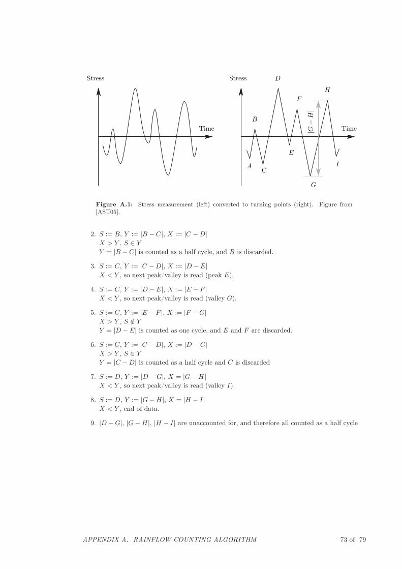
Time
A
B
C
D
E
F
G
H
I
Time
Stress Stress
|G−H|
Figure A.1: Stress measurement (left) converted to turning points (right). Figure from[AST05].
2. S := B, Y := |B − C|, X := |C −D|
X > Y , S ∈ Y
Y = |B − C| is counted as a half cycle, and B is discarded.
3. S := C, Y := |C −D|, X := |D − E|
X < Y , so next peak/valley is read (peak E).
4. S := C, Y := |D − E|, X := |E − F |
X < Y , so next peak/valley is read (valley G).
5. S := C, Y := |E − F |, X := |F −G|
X > Y , S /∈ Y
Y = |D − E| is counted as one cycle, and E and F are discarded.
6. S := C, Y := |C −D|, X := |D −G|
X > Y , S ∈ Y
Y = |C −D| is counted as a half cycle and C is discarded
7. S := D, Y := |D −G|, X = |G−H |
X < Y , so next peak/valley is read (valley I).
8. S := D, Y := |G−H |, X = |H − I|
X < Y , end of data.
9. |D −G|, |G−H |, |H − I| are unaccounted for, and therefore all counted as a half cycle
APPENDIX A. RAINFLOW COUNTING ALGORITHM 73 of 79

Appendix B
List of Acronyms
LQR Linear Quadratic Regulator
NREL National Renewable Energy Laboratory
SCADA Supervisory Control And Data Acquisition
74 of 79

APPENDIX B. LIST OF ACRONYMS 75 of 79
Bibliography
[Aeo08] Aeolus. Aeolus distributed control of large scale offshore wind farms. Fact Sheet,September 2008.http://ict-aeolus.eu/pub/fp7-fact-sheet-aeolus_en.pdf.
[Aeo10a] Aeolus. Simplified nrel5mw turbine. Webpage, August 2010. Detailed descriptionof NREL 5 MW Wind Turbine.http://www.ict-aeolus.eu/SimWindFarm/model-turbine.html.
[Aeo10b] Aeolus. Simwindfarm. Webpage, February 2010. Fast wind farm simulationenvironment for development of wind farm control algorithms.http://www.ict-aeolus.eu/SimWindFarm/.
[Aeo11] Aeolus. Experiment description. Aeolus Deliverable, April 2011.
[AST05] ASTM. Astm e 1049-85, standard practices for cycle counting in fatigue analysis.Designation: E 1049 85, Reapproved 2005.
[ÅW97] K. Åström and B. Wittenmark. Conputer-Controlled Systems. Prentice Hall, 3rdedition, 1997. ISBN 0-13-314899-8.
[BJS+11] B. Biegel, M. Juelsgaard, J. Stoustrup, M. Kranning, and S. Boyd. Wind turbinepitch optimization. Submitted to The 2011 IEEE Multi-Conference on Systems and
Control, 2011.
[Boy10] S. Boyd. Primal and dual decomposition. Lecture Notes, 2010. Stanford University,http://www.stanford.edu/class/ee364b/lectures/decomposition_slides.pdf.
[BSJB01] T. Burton, D. Sharpe, N. Jenkins, and E. Bossanyi. Wind Energy Handbook. Wiley,2001.
[Bul01] S. R. Bull. Renewable energy today and tomorrow. In Proceedings of the IEEE,
vol. 89, no. 8, August 2001.
[BV04] S. Boyd and L. Vandenberghe. Convex Optimization. Cambridge University Press,1st edition, 2004. ISBN 978-0-521-83378-3.
[Cou08] Ian Couchman. Plan for performance assessment. Aeolus deliverable 5.5, April 2008.
[GL00] T. Glad and L. Ljung. Control Theory, Multivariable and Nonlinear Methods.Taylor & Francis, 1st edition, 2000. ISBN 0-7484-0878-9.
[GSK+10] Jacob Deleuran Grunnet, Mohsen Soltani, Torben Knudsen, Martin Kragelund,and Thomas Bak. Aeolus toolbox for dynamic wind farm model, simulation andcontrol. In Proc. of the 2010 European Wind Energy Conference, 2010.
76 of 79
BIBLIOGRAPHY
[Ham06] K. Hammerum. A fatigue approach to wind turbine control. 2006. Master’s Thesisprepared at Vestas Wind Systems.
[HSBF05] A. D. Hansen, P. Sørensen, F. Blaabjerg, and I. Florin. Grid support of a windfarm with active stall wind turbines and ac grid connection. Wind Engineering,(9):341–359, 2005.
[JBMS09] J. Jonkman, S. Butterfield, W. Musial, and G. Scott. Definition of a 5-mwreference wind turbine for offshore system development. Technical report, NationalRenewable Energy Laboratory, 2009.http://www.nrel.gov/wind/pdfs/38060.pdf.
[JPP08] M. Jelavić, V. Petrović, and N. Perić. Individual pitch control of wind turbinebased on loads estimation. Industrial Electronics, 2008. IECON. 34th Annual
Conference of IEEE, November 2008.
[KBS09] Torben Knudsen, Thomas Bak, and Mohsen Soltani. Distributed control oflarge-scale offshore wind farms. In European Wind Energy Conference and
Exhibition (EWEC) 2009, Marseille, France, 2009.
[Lue84] D. G. Luenberger. Linear and Nonlinear Programming. Addison-Wesley, 2ndedition, 1984. ISBN 0-201-15794-2.
[MMR11] Daria Madjidian, Karl Mårtensson, and Anders Rantzer. A distributed powercoordination scheme for fatigue load reduction in wind farms. Submitted to
American Control Conference, San Francisco, June 2011.
[MR09] Karl Mårtensson and Anders Rantzer. Gradient methods for iterative distributedcontrol synthesis. In Proceedings of the 48th IEEE Conference on Decision and
Control, Shanghai, China, December 2009.
[MR10] Karl Mårtensson and Anders Rantzer. Sub-optimality bound on a gradient methodfor iterative distributed control synthesis. In Proc. 19th International Symposium
on Mathematical Theory of Networks and Systems, Budapest, Hungary, July 2010.
[NCVT10] S. Nourdine, H. Camblong, I. Vechiu, and G. Tapia. Comparison of wind turbinelqg controllers using individual pitch control to alleviate fatigue loads. 18th
Mediterranean Conference on Control & Automation, June 2010.
[Ofg09] Ofgem. Thanet offshore transmission assets. Technical report, 2009.http://www.ofgem.gov.uk/Networks/offtrans/rott/Documents1/Thanet%20-%20Project
[Ran09] Anders Rantzer. Dynamic dual decomposition for distributed control. InProceedings of American Control Conference, St. Louis, June 2009.
[SF01] R. I. Stephens and H. O. Fuchs. Metal Fatigue in Engineering. John Wiley & Sons,Inc., 2nd edition, 2001. ISBN 0-417-51059-9.
[SJBMV] V. Spudić, M. Jelavić, M. Baotić, and N. Perić M. Vasak. Deliverable 1.6: Plan forvalidation of control strategies. Public Aeolus Deliverables.
[SJBMV07] V. Spudić, M. Jelavić, M. Baotić, and N. Perić M. Vasak. Deliverable 3.3:Reconfigurable control extension. Public Aeolus Deliverables, 2007. University ofZagreb.
[SKB09] Mohsen Soltani, Torben Knudsen, and Thomas Bak. Modeling and simulation ofoffshore wind farms for farm level control. In European Offshore Wind Conference
and Exhibition (EOW) 2009, Stockholm, Sweden, 2009.
BIBLIOGRAPHY 77 of 79

BIBLIOGRAPHY
[Spu] V. Spudić. Hierarchical wind farm control for power/load optimization. Aeolus
Deliverable.
[Sti08] M. Stiebler. Wind Energy Systems for Electric Power Generation. Springer, 2008.
[Swi10] John Swigart. Optimal controller synthesis for decentralized systems. Ph.D.Dissertation, Stanford University, December 2010.http://junction.stanford.edu/~jswigart/publications/swigart_phd_dissertation.pdf.
[Ves11] Vestas. Aeolus test campaign at thanet offshore wind farm, uk. Technical report,Vestas Wind Systems, 2011.
[WWB10] H. Wang, W. Wang, and L. Bin. Application of individual pitch controller forflicker reduction on variable speed wind turbines. Power and Energy Engineering
Conference (APPEEC), 2010 Asia-Pacific, March 2010.
[XXZ+08] Y. Xingjia, W. Xiaodong, X. Zuoxia, L Yingming, and L. Jun. Individual pitchcontrol for variable speed turbine blade load mitigation. Sustainable Energy
Technologies, ICSET 2008. IEEE International Conference., November 2008.
78 of 79 BIBLIOGRAPHY