Distortion Analyzer – a New Tool for Assessing and Improving

Electrodynamic Transducer

Wolfgang Klippel

KLIPPEL GmbH, Aussiger Str. 3, 01277 Dresden, Germany www. klippel.de

Abstract: The dominant nonlinear distortions in loudspeakers, headphones and other actuators are predictable and are closely related with the general principle, particular design, materials and assembling techniques applied to the transducer. The Distortion Analyzer uses novel system identification techniques to measure the large signal parameters of the expanded loudspeaker model, the instantaneous state signals and the distortion components generated by each nonlinearity. This information is crucial for assessing the performance of transducer in the large signal domain as well as for finding the physical causes of the distortion to improve the transducer in respect with sound quality, weight, size and cost. 1 INTRODUCTION

At higher amplitudes most electrodynamic actuators behave as a time-variant and nonlinear system producing additional distortion components in the output signal [1 – 17]. To assess the nonlinear behavior quantitatively we usually apply spectrum analysis to evaluate the harmonic or intermodulation components in the output signal for multi-tone excitation input. Cross-correlation techniques have been introduced to measure the coherence between input and output signal which describes how good the transfer behavior of the transducer can be explained by a linear system. However, noise corrupting the measurement also deteriorates the coherence. All of the straightforward techniques used so far are not capable in measuring dynamically the particular nonlinearity inherent in the transducer and to quantify their contribution to the total distortion. However, in order to improve the transducer in the large signal domain we have to analyze the nonlinear distortion to understand by which nonlinear mechanism it is generated. Thus, distortion analysis turns out to be basically identification of the transducer nonlinearities. A new measurement system is required which fills the gap between loudspeaker theory and praxis. This paper describes the first implementation of the

1

system identification in the Distortion Analyzer 1 and practical applications to the diagnosis of a woofer system.

2 TRANSDUCER MODEL

At low frequencies electrodynamic actuators such as woofers, shakers and headphones can be modeled successfully by an electro-mechanic equivalent circuit comprising lumped elements and characterized by state quantities. 2.1 State Quantities The state of the transducer can be described by using the following quantities x(t) displacement of the voice coil, v(t) velocity of the voice coil, i(t) the electric input current, u(t) the driving voltage at loudspeaker terminals, P(t) real electric input power, TV(t) temperature of the voice coil temperature, TM(t) temperature of the magnet structure, TA temperature of the cold loudspeaker (ambient temperature), ∆TV(t)= TV(t)-TA increase of voice coil temperature and ∆TM(t) = TM(t)-TA increase of the temperature of magnet structure. 2.2 Linear Elements

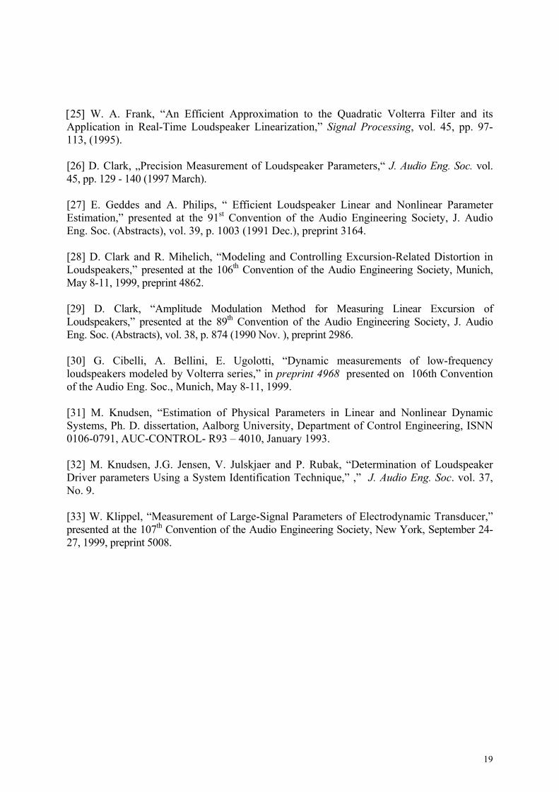
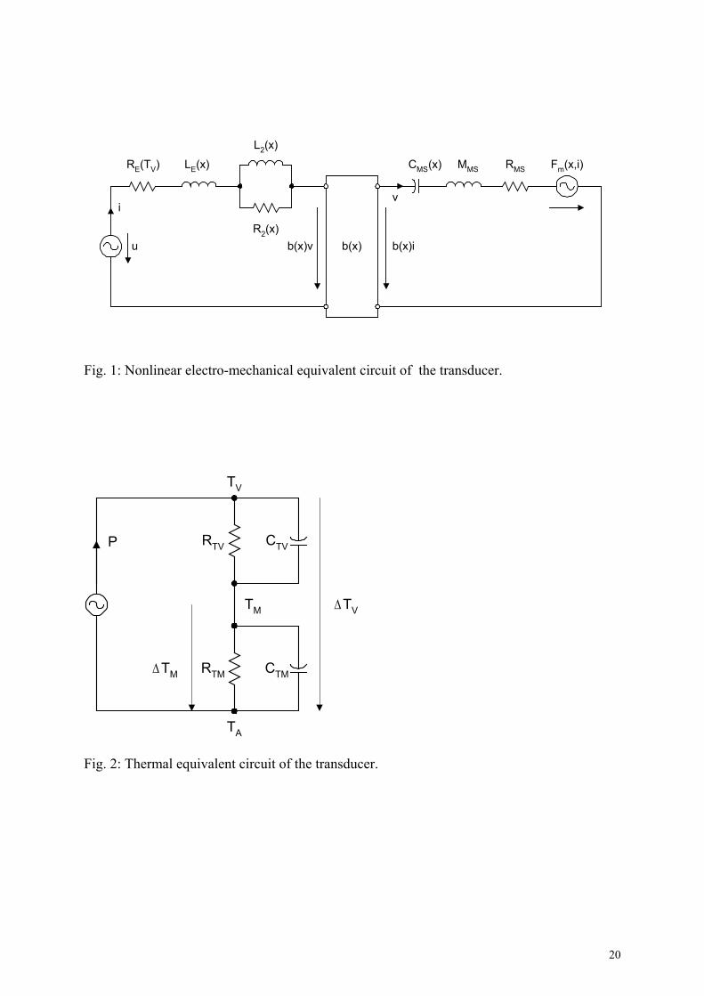
The relationship between those state signals is represented by an electromechanical and a thermal equivalent circuit as shown in Fig. 1 and 2. Some of the lumped elements have parameters which are almost independent on time and on any loudspeaker state. In congruence with linear loudspeaker theory they are defined as constant parameters:

MMS mechanical mass of driver diaphragm assembly including voice-coil and air load, RMS mechanical resistance of total-driver losses, RTV thermal resistance of path from coil to magnet structure, RTM thermal resistance of magnet structure to ambient air, CTV thermal capacitance of voice coil and nearby surroundings, CTM thermal capacitance of magnet structure. The time-constant τTV=RTVCTV representing the voice coil is in the range of a few seconds whereas the time-constant τTM=RTMCTM reaches values up to an hour. 2.3 Nonlinear Elements

2

The dominant nonlinearities are modeled by displacement depending parameters such as b(x) instantaneous electrodynamic coupling factor (force factor of the motor)

defined by the integral of the magnetic flux density B over voice coil length l,

CMS(x,t)=1/ KMS(x,t) compliance of driver suspension + air load (the inverse of stiffness), LE(x) part of voice coil inductance which is independent on frequency, ZL(x,s) electric impedance representing the influence of eddy currents, which

can be approximated by

Z x s R x L x sR x L x sL ( , ) ( ) ( )

( ) ( )=

+2 2

2 2

(1)

where s=2πfj Laplace Operator using frequency f and j=√-1, L2(x) represents the para-inductance of the voice coil and R2(x) the electric resistance due to additional losses caused by eddy currents. Since of the inductance parameters LE(x), L2(x) and R2(x) are directly related with the magnetic field generated by the voice coil current i(t), it may be assumed that these parameters vary in the same way on the displacement x:

Z x sZ s

L xL

L xL

R xR

L

L

E

E

( , )( , )

( )( )

( )( )

( )( )0 0 0

2

2

2

2

= = =0

(2)

This variation of the magnetic field energy on voice coil displacement also generates a reluctance force Fm(x,i) which can be approximated by

F x i i t L xxm

E( , ) ( ) ( )≈

2

2∂

∂.

(3)

The force factor b(x) and the inductance parameters depend on the instantaneous displacement only and are almost time-invariant as long as the rest-position of the voice coil is not changed. However, stiffness kMS(x,t) of the mechanical suspension is also a function of the preceding displacement values to explain fatigue, hystereses, creep and temporal changes. 2.4 Time-variant Elements

The electric resistance RE(TV) of the voice coil is a linear but time-varying parameter which depends on the instantaneous voice coil temperature TV.

3

2.5 Derived Loudspeaker Parameters

For the analysis and synthesis of loudspeaker system it is convenient to use special parameters derived from the physical parameters such as the mechanical resonance frequency of the driver

f xM C xS

M S M S

( )( )

=1

2π (4)

the loss factor of driver at fs and at voice coil temperature TV considering electrical resistance RE(TV) only defined by

Q T x f x M R Tb xE S V

S M S E( , ) ( ) ( )( )

=2

2Vπ , (5)

the loss factor of driver at fs considering driver non-electrical resistances only defined by

Q xf x R C x

f x MRM S

S M S M S

S M

M S

( )( ) ( )

( )= =

12

2π

Sπ , (6)

the total loss factor at fs and voice coil temperature TV including all system resistances defined by

Q T x Q x Q T xQ x Q T xT V

M S E S V

M S E S V

( , ) ( ) ( , )( ) ( , )

=+

, (7)

and the volume of air

V x c S C xA S D M S( ) ( )= ρ 02 2 (8)

having the same acoustic compliance as the driver suspension with the density of air (ρ0=1.18 kg/m3 ) and the velocity of sound in air c=345 m/s. Clearly these parameters are not constant but depend on the instantaneous state of the transducer (displacement x, the voice coil temperature TV). 2.6 Relationship to Small Signal Modeling

The expanded model corresponds with the results of traditional linear modeling if the amplitude of the state signals is sufficiently small such that the variation of the nonlinear parameters and the heating of the voice coil can be neglected. Then the derived parameters in Eqs. 4 - 8 coincide with the well-known Thiele-Small parameters [1-3].

4

3 IDENTIFICATION OF THE MODEL

The Distortion Analyzer measures the free parameters and state signals in the equivalent circuits by system identification techniques based on digital signal processing [18-24]. 3.1 Sensing Physical Quantities

To apply the model to a particular transducer we have to estimate the free parameters in such a way that our theoretical model describes the behavior of the real transducer as precisely as possible. The behavior of the transducer can be characterized by the state signals found in the equivalent circuits. Transducers in normal operation mode are usually driven by a low impedance source and the electric voltage at the terminals is used as an excitation input. The remaining states depend on the input signal and the measurement of at least one state signal is necessary to identify the model successfully. The measurement of the displacement, velocity or acceleration of the voice coil require an expensive sensor. The direct measurement of the voice coil temperature is also impractical because the moving voice coil in the gap is not accessible. However, the current signal i(t) is a state signal which can easily be measured and provides sufficient information about the mechanical and thermal mechanisms in the transducer. The system identification based on current measurement is illustrated in Fig. 3. Both the transducer and the model are provided with an excitation signal. The difference between measured current i(t) and estimated current i’(t) is used as error signal e(t) for the adjustment of the free model parameters. Due to the impedance measurement the Distortion Analyzer identifies electric equivalent circuit presented in Fig. 4 primarily. In a second step the electrical capacitance representing moving mass

C x Mb xM E S

M S( )( )

= 2 , (9)

the electrical inductance of driver compliance

L x C x b x b xK xC E S M S

M S

( ) ( ) ( ) ( )( )

= =22

, (10)

the electrical resistance due to driver suspension

R x b xRE S

M S

( ) ( )=

2

(11)

and the current source representing the electromagnetic drive

i x i F x ib xmm( , ) ( , )( )

= (12)

5

are transformed into mechanical parameters represented by Fig. 1 using the force factor b(x). 3.2 Adaptive Parameter Estimation

The model is adjusted to the particular transducer in a optimal way when the magnitude of the error becomes minimal. The Distortion Analyzer solves this optimization problem by using an adaptive scheme as described in [33]. In this approach the transducer model is implemented in a DSP as a digital system and gradient signals are correlated with the error e(t) to update the parameter estimates iteratively. This approach has the advantage that the system identification can be accomplished on-line while the transducer is operated under normal working condition and the variation of the states and parameters can be monitored over time.

3.3 System Components

The Distortion Analyzer 1 which is optimized for transducers with a resonance frequency between 10-200 Hz consists of the following components: - processor unit - audio power amplifier - cable for connecting speaker and amplifier - IBM compatible computer with USB interface under Windows 98 - analyzer and simulation software The processor unit is a stand-alone system capable for making long-term measurements of loudspeakers with a minimum of equipment. In addition to the analog hardware (AD/DA and current and voltage sensors) the processor hosts sufficient DSP processing power to do the nonlinear calculations on-line. As a stand-alone system it also has a minimal user-interface to start parameter measurements without computer and to display important information permanently. The parameter and state information are sampled regularly at fixed intervals and stored in a database inside the processor unit. The serial interface USB makes it possible to connect one or more processor units to a computer and to investigate the reported measurement results more thoroughly. An AC-coupled audio amplifier is required for driving the transducer in the large signal domain. The Distortion Analyzer supervises the linearity of the amplifier and stops the measurement when the amplifier starts with limiting. 3.4 Measurement Condition

6

3.4.1 Mounting the Transducer

In the first version of the Distortion Analyzer the transducer should be measured under conditions such that the mechanical system including any acoustical load can be represented as a second-order system in accordance with the modeling above. Woofers may be operated in free air or in a sealed enclosure. Knowing the volume of the enclosed air the parameters of the driver can be separated from the results measured at the total system. Shakers should be mounted on a solid platform to avoid any higher-order modes which have not yet considered in the model. There is further research going on to allow system identification of transducers connected to an acoustical or mechanical system with higher complexity such as vented- or bandpass system. This measurements may be helpful to identify port nonlinearities and to investigate their influence on the driver more thoroughly.

In any case, the measurement of the woofer in free air is very convenient because the mechanical properties can be measured with a minimum of electric power applied to the loudspeaker system while producing minimal sound pressure. A special stand proved to be convinient to mount woofers in a vertical position and to measure the displacement of the diaphragm by a laser displacement meter or to use a microphone in near field measurements. Because the acoustic environment in greater distance has a minor influence on the loudspeaker parameter, the measurement can also be performed in a normal working room or in a power test room.

An additional mass Madd can be fasten on the diaphragm to measure the shift of the resonance frequency and to identify the moving mass MMS of the transducer from the shift of the resonance frequency. However, techniques approved for traditional linear measurements showed to be not practical at high displacements. 3.4.2 Excitation signal 3.4.2.1 Spectral and amplitude distribution

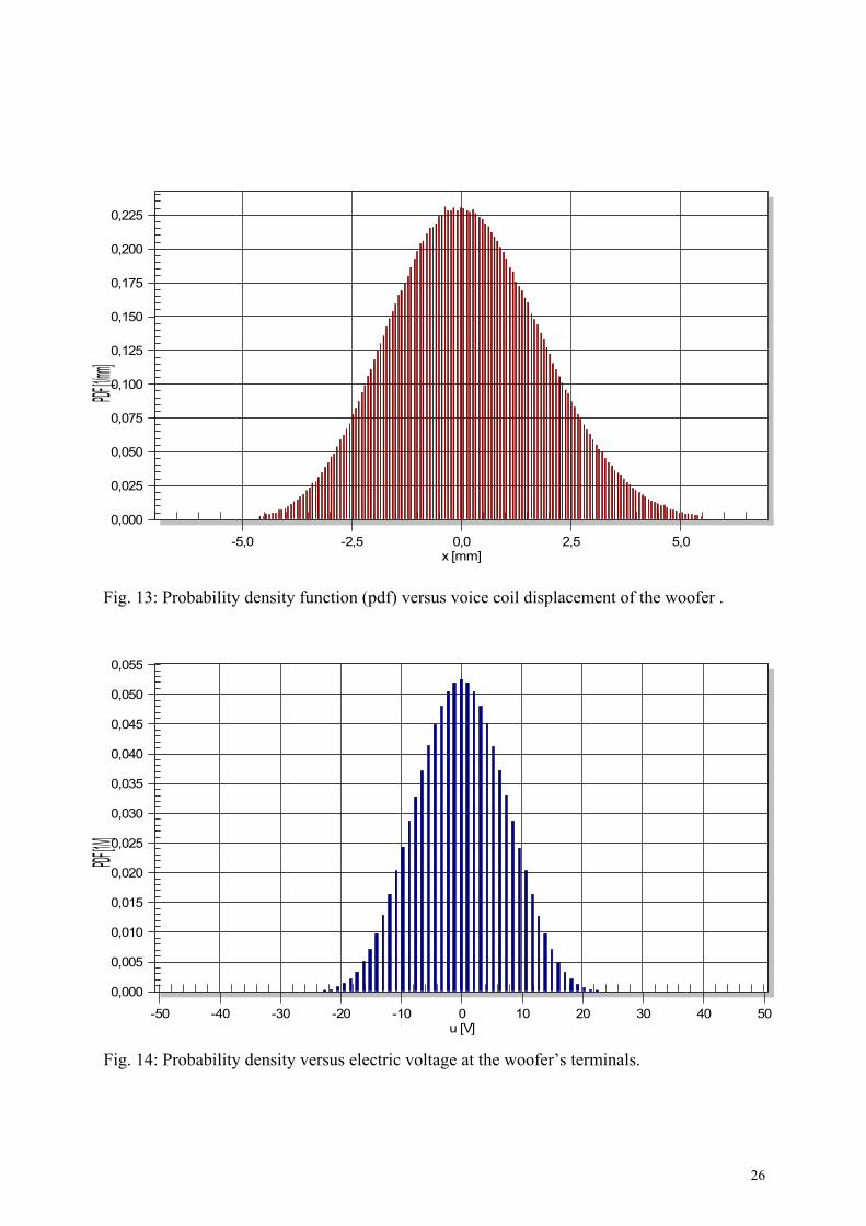
This Distortion Analyzer needs an excitation signal with sufficient amplitude and spectral properties to identify the transducer completely. A single sinusoidal signal with constant frequency and amplitude would allow to identify a system with two free parameters only. Clearly a multi-tone signal at high frequencies or a flute concert without any bass content would not generate high excursions of the voice coil and would not produce enough nonlinear distortion which is the basis for detecting the transducer’s nonlinearities. Most of ordinary audio signals such as full orchestra music or pop music give persistent excitation but require a signal source (CD-player). However, an artificial noise signal used for simulating program material as specified in IEC 60268-1 is preferable to transducer measurements. This signal can easily be generated in a DSP with desired properties in respect with spectral properties and reasonable amplitude distribution and enables the system identification to find the optimal parameters in a short time. Fig. 13 shows the probability density function (pdf) of the displacement for the noise which has a similar amplitude distribution as an ordinary audio signal.

7

3.4.2.2 Signal Amplitude

Although the transducer is measured in the large signal domain up to the physical limits it is expected from the Distortion Analyzer to ensure a nondestructive measurement. Sometimes the power handling capacity or the maximal displacement of a valuable prototype are not available or far away from the true values. Therefore, the Distortion Analyzer has to detect the safe working range of the particular transducer automatically. That is possible because the identified models give sufficient indications about the instantaneous load imposed to the transducer. The maximal power handling capacity in respect with the thermal load can easily be determined by monitoring the increase of the voice coil temperature ∆TV(t). The mechanical load put on the suspension corresponds with the variation of the compliance CMS(x) defined by

V C xCC x x x

M S

M S

=

− < <m in ( )

( )m a x m a x 0.

(13)

Most woofer systems can handle temporary decreases down to 20% without any damage. In a reasonable transducer design the mechanical capability is limited by the spider or at least by the surround but a contact of the voice coil former with the back plate should be avoided in any case.

The maximal variation of the force factor

V b xbB x x x

=

− < <m in ( )

( )m a x m a x 0,

(14)

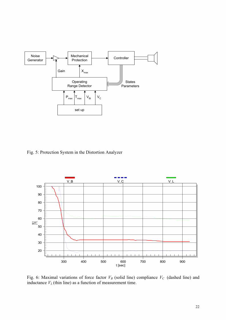
is another useful criterion to detect the working range of the transducer. The Distortion Analyzer uses this information in a protection system illustrated in Fig. 5. The external audio signal or the internally generated noise signal is fed via a gain control unit, mechanical protection system and the controller to the transducer. At the start of the measurement procedure the excitation signal is small where even an unidentified transducer can be operated safely. Slowly the gain of the excitation signal is increased and the voice coil temperature, the maximal variations of the nonlinear parameters CMS(x), b(x) and the true electric input power P is measured simultaneously. When one of these criteria exceeds a user defined threshold the gain of the excitation signal is attenuated to find the optimal working range. In order to protect the transducer against mechanical destruction, the envelope of the displacement signal is calculated to predict the next peak value. In the case of an imminent overload situation the very low frequency components of the excitation signal are attenuated by shifting the cut-off frequency of a variable high-pass filter in time to keep the excursion in the allowed working range. For each protection criteria a limit value can be specified in the user interface:

∆TVmax allowed increase of voice coil temperature ∆TV, VBmax allowed maximal variation of the force factor VB, VCmax allowed maximal variation of the mechanical compliance VC, Pmax maximal electric input power.

8

The first three limit values ∆TVmax, VBmax and VCmax are general setup parameter independent on the maximal displacement xmax and the power P admissible for the particular driver. The maximal electric input power Pmax can be used as a more restrictive protection parameter which is independent on the identification of the thermal and nonlinear mechanisms. 3.5 Execution of the Measurement 3.5.1 User Interaction

After placing the transducer in a vertical measurement position and connecting its terminals, the measurement is started either from the stand-alone processing unit or from a connected computer. Based on the general protection parameters defined in the user set up no additional input parameters are required. The safe range of operation is found for any woofer between a small 3 inch multimedia speaker and a 18 inch woofer used in professional application automatically. 3.5.2 Measurement Procedure The measurement procedure is organized in 5 steps processed sequentially. 3.5.2.1 1st step: Amplifier Test

Before driving the loudspeaker with the excitation signal the additional equipment (power amplifier, cables, clamps) are checked in respect with

- connectivity - gain of the amplifier - polarity (180 degree phase shift) of the signal - nonlinear distortion produced by the amplifier - linear transfer function (phase and amplitude response)

If the test is not successful the controller goes automatically into an exception state where further processing is aborted and a malfunction message is released. 3.5.2.2 2nd step: Small-Signal Measurement

After passing the amplifier test, the loudspeaker is supplied with a small amplitude excitation signal. Since the variations of the nonlinear parameters and the heating of the voice coil can be neglected, the identified parameters corresponds with the results of a traditional small-signal measurement. The voice coil resistance related to the ambient temperature TV = TA measured in this step is used as a reference to estimate the increase of voice coil temperature ∆TV = TV - TA in the following measurements.

9

3.5.2.3 3rd step: Detection of Operation Range

After convergence of the linear parameter estimation the thermal and nonlinear parameters are estimated in the large signal domain by increasing slowly the amplitude of the excitation signal until one of the protection criteria reaches the predefined limit values and the safe range of operation is detected. 3.5.2.4 4th step: Detection of Thermal Parameters

Driving the loudspeaker in the allowed working range the thermal resistance RTV and capacity CTV of the voice coil are measured by attenuating the speaker’s input power for a short period of 2 min and monitoring the voice coil temperature ∆TV. 3.5.2.5 5th step: Slow Speed Learning

Finally the learning speed of the update algorithm is reduced to minimize the influence of measurement noise on the parameter estimates. The instantaneous states and parameters are stored in the data base at a reduced sample rate to monitor long-term variations of the transducer parameters and to measure the thermal resistance RTM and capacitance CTM of the magnet structure. 4 RESULTS

The Distortion Analyzer provides permanently general control information about the progress of the system identification as well as physical information about the state and parameters of transducer. In addition to the most important information displayed at the processing unit, a computer allows access to further details. All of this information is also stored in the database and makes it possible to investigate the identification process systematically. 4.1 General Control Information

The general control unit gives information about the measurement time, mode of operation, progress in the parameter updating and releases warnings in malfunction situations. The protection criteria ∆Tv, VB, VC and P contrasted to the corresponding limit values ∆Tvmax, VBmax, VCmax and Pmax report about the progress in working range detection. Fig. 6 shows the maximal variations of force factor VB, compliance VC and inductance VL versus measurement time where

V L xLL x x x

E

E

=

− < <m in ( )

( )m a x m in 0.

(15)

10

The other protection criteria electric power P and increase in voice coil temperature ∆Tv are presented in Fig 7. In this example the variation of VC reaches the allowed limit of VCmax=20% first showing that the allowed working range is limited by the mechanical suspension.

The maximal peak values of the error signals used in the identification of the transducer, in amplifier check and in the adjustment of the optional laser displacement meter are expressed as relative quantities. These error signals does not only reflect imperfections in the modeling but also the occurrence of measurement noise and minor time delay and phase shifts caused by the DA/AD conversion. Fig. 8 shows the peak value of the identification error for the particular transducer versus measurement time. 4.2 Transducer Parameters 4.2.1 Small Signal Parameters 4.2.1.1 Electrical Parameters

The first data which becomes available are the parameters of the electrical equivalent circuit in Fig. 4 at the rest position (x=0) of the cold voice coil (∆Tv =0) comprising the electric dc resistance RE(0 ), and the parameters of the para-inductance LE(0) ,L2(0),R2(0) and the mechanical elements represented in the electric domain by CMES(0) ,LCES(0) and RES(0) listed in the third column of Table I. 4.2.1.2 Mechanical and Acoustical Parameters

To identify the force factor and the other elements in the mechanical domain we need additional information that are not available in the electric impedance of the transducer. There are different ways to provide this information to the Distortion Analyzer. It is possible to import the force factor and/or the moving mass determined by traditional methods based on two impedance measurements of the driver with and without additional mass or with or without enclosure. However, it is more convenient to measure the displacement of the diaphragm by using an inexpensive laser and to supply this signal to the Distortion Analyzer. If the measured displacement signal correlates significantly with the reference displacement of the model, the parameter transformation is performed automatically.

In order to calculate the electroacoustical efficiency η and the reference sound pressure in axis the diaphragm area SD has to provided as an additional geometric driver parameter. 4.2.2 Large Signal Parameters 4.2.2.1 Nonlinear Parameters

After the model is identified in the rest position of the voice coil, the nonlinear and

11

thermal characteristics are identified in the 3rd step of the measurement procedure while the gain of the excitation signal is permanently increased to find the limits of the working range. The current parameter estimates on the nonlinear elements LE(x), L2(x), R2(x), b(x), CMES(x), LCES(x), RES(x), CMS(x), KMS(x) are displayed as a function of the displacement in the range -xmax < x < xmax where xmax is the maximal allowed displacement detected by the protection system. If the mechanical system has been identified by using an import parameter or laser displacement meter all of these parameters can be expressed in their physical units depending on the displacement in mm. If this information is not yet available the mechanical compliance and the force factor are expressed as relative quantities CMS(xrel)/CMS(0) and b(xrel)/b(0), respectively, to show the nonlinear characteristic of these and the other parameters LE(xrel), L2(xrel), R2(xrel), CMES(xrel) ,LCES(xrel), RES(xrel) as a function of the relative displacement (xrel =x/xmax).

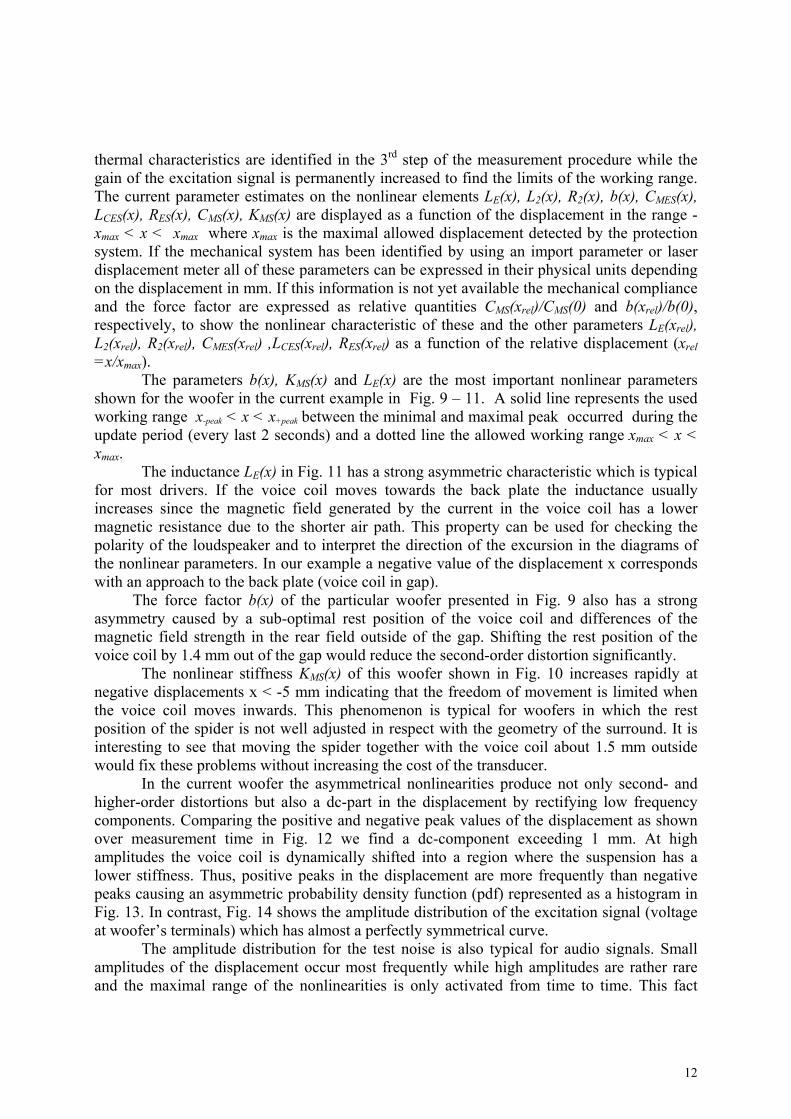
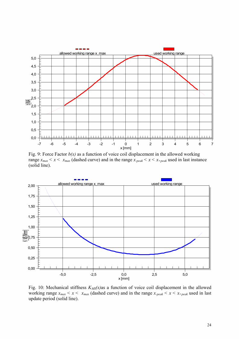
The parameters b(x), KMS(x) and LE(x) are the most important nonlinear parameters shown for the woofer in the current example in Fig. 9 – 11. A solid line represents the used working range x-peak < x < x+peak between the minimal and maximal peak occurred during the update period (every last 2 seconds) and a dotted line the allowed working range xmax < x < xmax.

The inductance LE(x) in Fig. 11 has a strong asymmetric characteristic which is typical for most drivers. If the voice coil moves towards the back plate the inductance usually increases since the magnetic field generated by the current in the voice coil has a lower magnetic resistance due to the shorter air path. This property can be used for checking the polarity of the loudspeaker and to interpret the direction of the excursion in the diagrams of the nonlinear parameters. In our example a negative value of the displacement x corresponds with an approach to the back plate (voice coil in gap).

The force factor b(x) of the particular woofer presented in Fig. 9 also has a strong asymmetry caused by a sub-optimal rest position of the voice coil and differences of the magnetic field strength in the rear field outside of the gap. Shifting the rest position of the voice coil by 1.4 mm out of the gap would reduce the second-order distortion significantly. The nonlinear stiffness KMS(x) of this woofer shown in Fig. 10 increases rapidly at negative displacements x < -5 mm indicating that the freedom of movement is limited when the voice coil moves inwards. This phenomenon is typical for woofers in which the rest position of the spider is not well adjusted in respect with the geometry of the surround. It is interesting to see that moving the spider together with the voice coil about 1.5 mm outside would fix these problems without increasing the cost of the transducer.

In the current woofer the asymmetrical nonlinearities produce not only second- and higher-order distortions but also a dc-part in the displacement by rectifying low frequency components. Comparing the positive and negative peak values of the displacement as shown over measurement time in Fig. 12 we find a dc-component exceeding 1 mm. At high amplitudes the voice coil is dynamically shifted into a region where the suspension has a lower stiffness. Thus, positive peaks in the displacement are more frequently than negative peaks causing an asymmetric probability density function (pdf) represented as a histogram in Fig. 13. In contrast, Fig. 14 shows the amplitude distribution of the excitation signal (voltage at woofer’s terminals) which has almost a perfectly symmetrical curve. The amplitude distribution for the test noise is also typical for audio signals. Small amplitudes of the displacement occur most frequently while high amplitudes are rather rare and the maximal range of the nonlinearities is only activated from time to time. This fact

12

explains why the identification of a linear system and the nonlinearities at small displacement can be accomplished within a few seconds but the measurement of the nonlinarities at the very end of the operating range takes a few minutes. In respect with the optimal parameter adjustment and the minimization of the error amplitude the amplitude distribution of the displacement is a kind of a weighting function. Imperfections in the modeling affect more the precision of the nonlinear parameters at high displacement than at small and medium values.

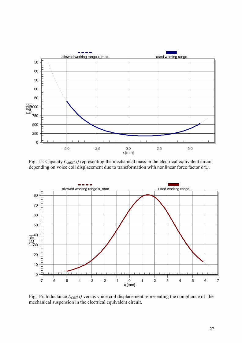
The remaining nonlinear parameters L2(x), R2(x), CMES(x), LCES(x) and RES(x) are closely related with the primary parameters b(x), KMS(x) and LE(x). According to Eq. (2) the para inductance L2(x) and the losses R2(x) due to eddy currents have the same characteristic as LE(x). The parameters CMES(x) ,LCES(x), RES(x), representing the mechanical elements in the electrical equivalent circuit are shown in Fig. 15 – 17. By transforming the moving mass MMS and the mechanical resistance RMS into the electric domain they become nonlinear elements depending on the squared force factor b(x)2 as shown in Eqs. 9 – 11. Thus the electric equivalent circuit gives a distorted picture of the mechanical elements and is less suitable for loudspeaker modeling in the large signal domain. More interesting are the resonance frequency fS(x), electric loss factor QES(TV,x), mechanical loss factor QMS(x) and the total loss factor QT(TV,x) which are presented in Fig. 18 – 21. According to Eqs. 4 – 7 all of these parameters depend on the nonlinear parameters b(x) and CMS(x) and vary with the instantaneous displacement. For instance, when the voice coil moves through the rest position the resonance frequency is only fS(0)=43Hz but increases to fS(x-peak)= 78 Hz at the peak value x-peak= -5mm happened in the last update period (within the preceding 2 sec) and would reach fS(-xmax)=105 Hz if the voice coil would be displaced to the allowed maximal value xmax = -7mm defined by the protection system.

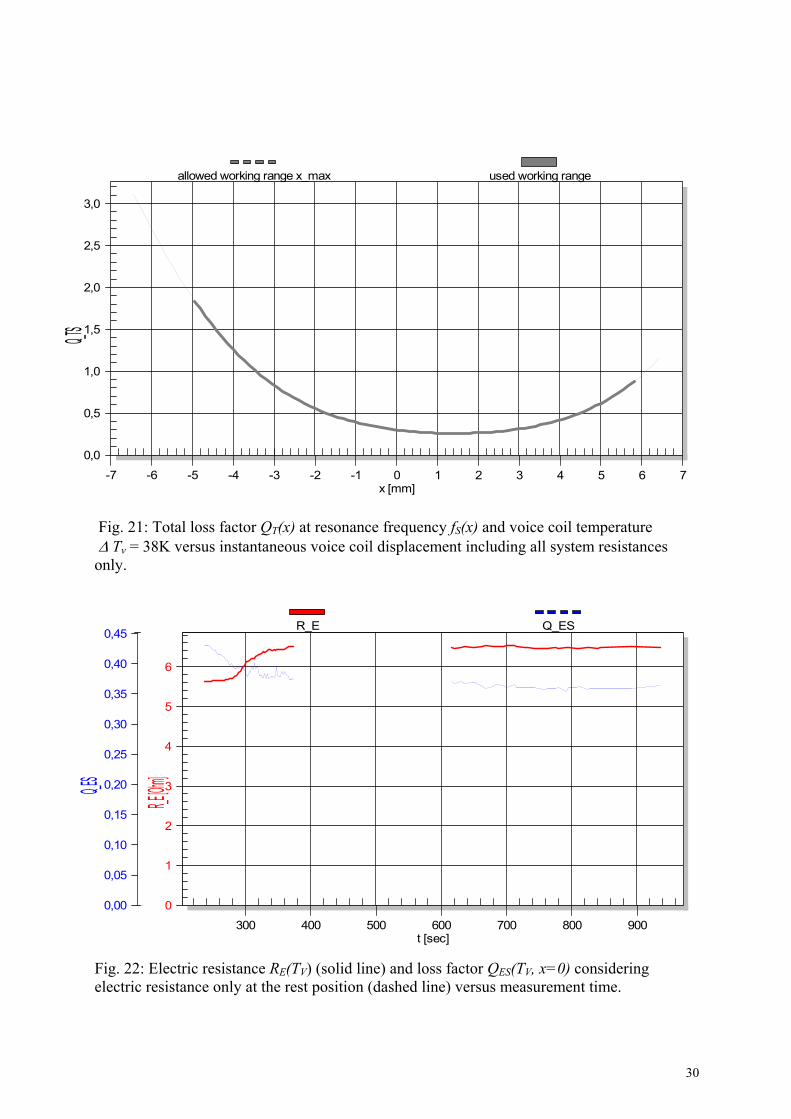
The loss factor QES(TV,x) at resonance frequency fS(x) considering electrical resistance RE(TV) at ∆ Tv = 38K only, varies dramatically with voice coil displacement. Only at very small displacements we have the high electrical damping QES(TV,0) ≈ 0.35 usually desired in the application which dominates the total QT(TV,0) ≈ 0.3. However, when the voice coil moves out of the gap the electric damping disappears literally resulting in a high QES(TV, -xmax) ≈ 9. Simultaneously, the mechanical QMS(x) also increases with fS(x) due to the nonlinear suspension resulting in a total system having a high QT(TV, -xmax) ≈ 1.8 at maximal displacement. However, the enormous rise of QT(TV, x) does not cause a similar increase of the amplitude response because the higher loss factor partly compensates for the reduced excitation of the driver due to the force factor decay b(x). These effects can be investigated in greater detail by numerical simulations based on the identified model. In order to represent the nonlinear parameters by a minimal set of parameters and to simplify the export to numerical simulations the force factor b(x), compliance CMS(x) and inductance LE(x) are expanded into a power series and the nonlinear coefficients are calculated which give the best fitting to primary data. Table II gives such a set of data for the woofer used in our example. 4.2.2.2 Parameters at the Rest Position

To compare the results of large signal measurements with the results of the small signal measurements we consider the values of the nonlinear parameters at x=0 when the voice coil passes the rest position. The parameters of the warm driver at full drive are

13

presented in the first column of Table I. Some of the parameters such as force factor b(0), inductance LE(x) and moving mass MMS are very close to the linear parameters in the third column measured in the small signal domain. Of course the resistance RE(TV) of the warm driver is higher then RE(TA) of the cold driver. Fig. 22 shows the RE(TV) and the loss factor QES(TV, x=0) at the rest position versus measurement time. For the particular woofer used in the example, the variations of QES(TV, x=0) due to the increase of voice coil temperature in Fig. 22 are negligible in comparison to the variations caused by voice coil displacement as shown in Fig. 19.

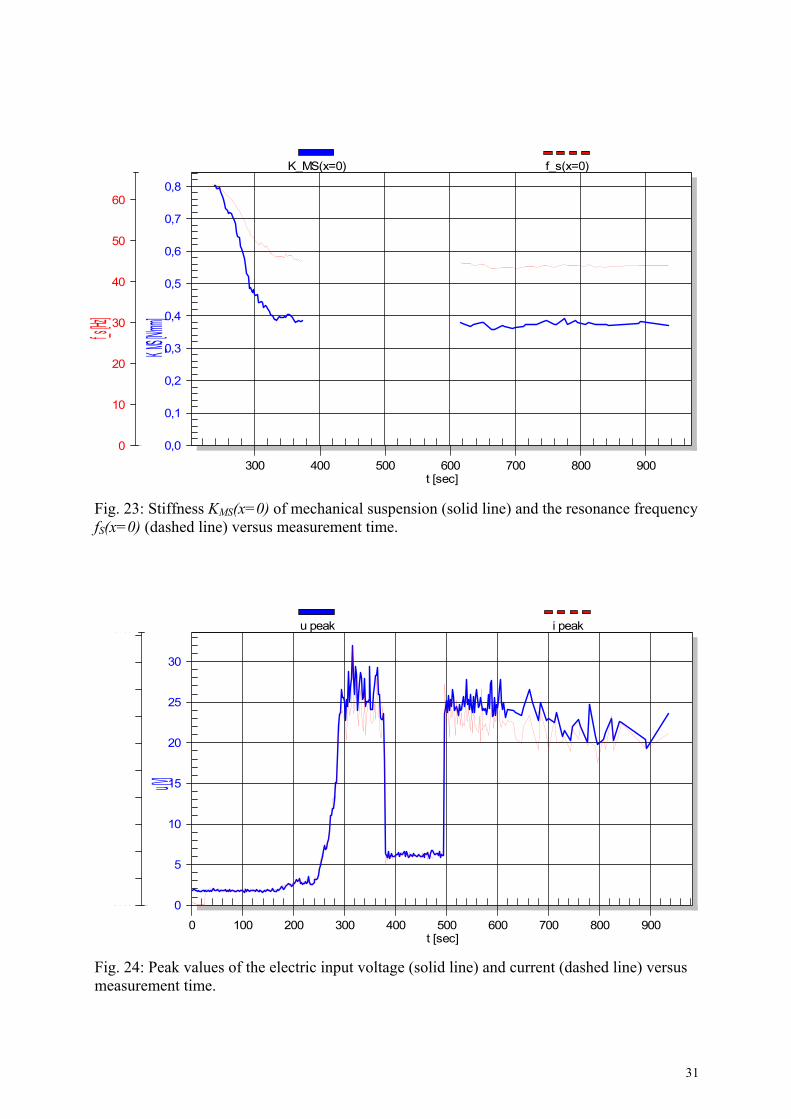
In the second column of Table I the influence of voice coil temperature on the linear loudspeaker parameters is compensated by using instead of resistance RE(TV ) of the warm transducer the initial value RE(TA) of the transducer at ambient temperature. There are still some differences in the loss factors due to higher values of mechanical resistance RMS and stiffness KMS(x=0) at high amplitudes. The occurrence of air turbulences in the gap and in the vent of the back plate and microscopic changes in the suspension might increase the mechanical losses at high amplitudes but these variations are still minor in comparison to the nonlinear damping caused by b(x) nonlinearity. More significantly is the fact that the driver’s suspension at the rest position becomes softer when the amplitude xpeak is increased. Fig. 23 shows the stiffness KMS(x=0) and the resonance frequency fS(x=0) versus measurement time in detail. In contrast to the irreversible parameter changes found at new woofers operating the first time under full load (break-in), the resonance frequency fS(x=0) approaches the initial value after reducing the amplitude of the excitation signal. This effect can be measured on most woofers (compare Fig. 1 in [26]) which use conventional design and spider materials. It seems that the mechanical suspension should be understood as a nonlinear system having some memory in which the stiffness KMS(x,t) depends not only on the instantaneous displacement but also on the previous history of the displacement signal exposed on the suspension a few seconds before. There is more research required to confirm the hypothesis and to explain these mechanisms by a physical model. 4.2.2.3 Thermal Parameters

The thermal parameters are identified from the time characteristic of the temperature ∆TV and the electric input power P stored in the database as shown in Fig. 7. In the 4th step of the measurement procedure the input power is reduced for 120 seconds and the thermal resistance RTV and capacity CTV of the voice coil are calculated from the early changes of the temperature curve since the time constant τTV of the voice coil is always much smaller than τTM . Using the voice coil parameters RTV and CTV , the thermal resistance RTM and the capacity CTM of the magnet are estimated from the further increase of the voice coil temperature recorded in the last 5th step of the learning procedure. For the particular loudspeaker the thermal parameters are: thermal resistance of path from coil to magnet structure, RTV= 2.31 K/W

thermal resistance of magnet structure to ambient air, RTM= 2.22 K/W thermal capacitance of voice coil and nearby surroundings, CTV= 23 J/K thermal capacitance of magnet structure. CTM= 310 J/K.

14

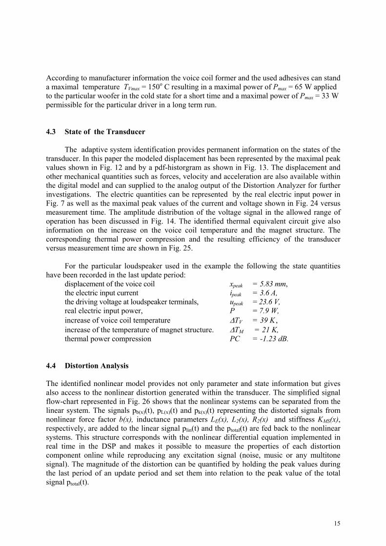
According to manufacturer information the voice coil former and the used adhesives can stand a maximal temperature TVmax = 150o C resulting in a maximal power of Pmax = 65 W applied to the particular woofer in the cold state for a short time and a maximal power of Pmax = 33 W permissible for the particular driver in a long term run. 4.3 State of the Transducer

The adaptive system identification provides permanent information on the states of the

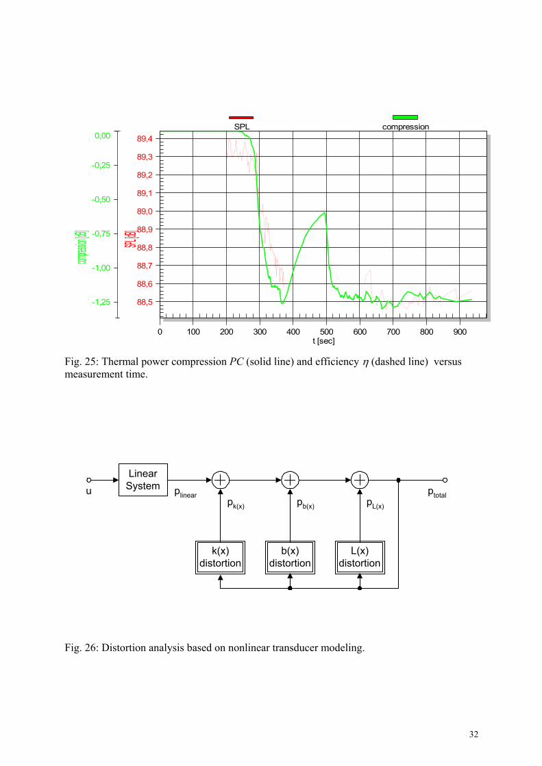
transducer. In this paper the modeled displacement has been represented by the maximal peak values shown in Fig. 12 and by a pdf-historgram as shown in Fig. 13. The displacement and other mechanical quantities such as forces, velocity and acceleration are also available within the digital model and can supplied to the analog output of the Distortion Analyzer for further investigations. The electric quantities can be represented by the real electric input power in Fig. 7 as well as the maximal peak values of the current and voltage shown in Fig. 24 versus measurement time. The amplitude distribution of the voltage signal in the allowed range of operation has been discussed in Fig. 14. The identified thermal equivalent circuit give also information on the increase on the voice coil temperature and the magnet structure. The corresponding thermal power compression and the resulting efficiency of the transducer versus measurement time are shown in Fig. 25.

For the particular loudspeaker used in the example the following the state quantities

have been recorded in the last update period: displacement of the voice coil xpeak = 5.83 mm, the electric input current ipeak = 3.6 A , the driving voltage at loudspeaker terminals, upeak = 23.6 V, real electric input power, P = 7.9 W, increase of voice coil temperature ∆TV = 39 K , increase of the temperature of magnet structure. ∆TM = 21 K, thermal power compression PC = -1.23 dB.

4.4 Distortion Analysis

The identified nonlinear model provides not only parameter and state information but gives also access to the nonlinear distortion generated within the transducer. The simplified signal flow-chart represented in Fig. 26 shows that the nonlinear systems can be separated from the linear system. The signals pb(x)(t), pL(x)(t) and pk(x)(t) representing the distorted signals from nonlinear force factor b(x), inductance parameters LE(x), L2(x), R2(x) and stiffness KMS(x), respectively, are added to the linear signal plin(t) and the ptotal(t) are fed back to the nonlinear systems. This structure corresponds with the nonlinear differential equation implemented in real time in the DSP and makes it possible to measure the properties of each distortion component online while reproducing any excitation signal (noise, music or any multitone signal). The magnitude of the distortion can be quantified by holding the peak values during the last period of an update period and set them into relation to the peak value of the total signal ptotal(t).

15

dppb x

b x

to ta l( )

( )= . (16)

dppL x

L x

to ta l( )

( )= . (17)

dppk x

k x

to ta l( )

( )= . (18)

These relative degrees of distortion specify the contribution of each primary

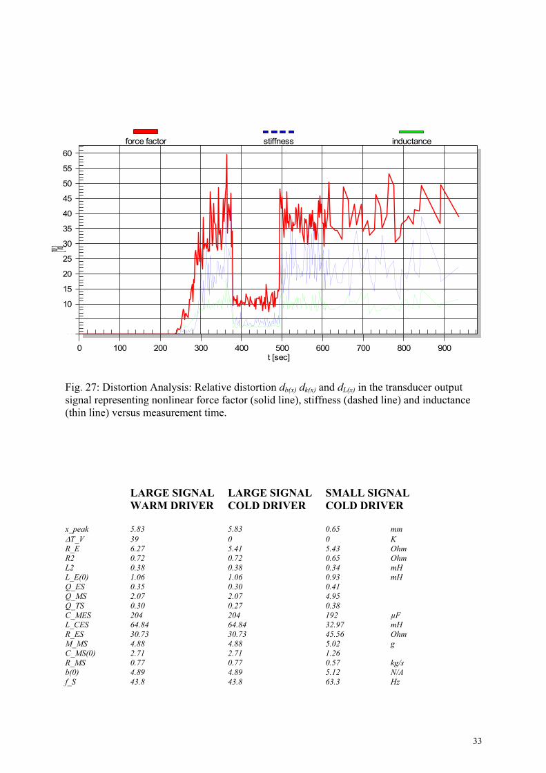
nonlinearity to the signal and are represented in Fig. 25 versus measurement time. Clearly, all of the distortion components rises with the amplitude of the excitation. At maximal amplitudes the particular woofer produces dominant force factor distortion exceeding 50 % signal amplitude due to the asymmetry in the motor structure and the low voice coil overhang. The contribution of the mechanical suspension only reaches 30 - 40 % mainly generated when the moving capability of the mechanical surround is limited at negative displacements. The nonlinear inductance produces about 10 % distortion in the reproduced sound which is still substantial in comparison to any other system (amplifier, AD-DA converter, ...) in the electroacoustic chain. The access to the separated nonlinear distortion signals as a time signal via analog output also allow more elaborate investigations such as spectral analysis and amplitude distribution.

5 CONCLUSION

Nonlinear system identification as performed by the Distortion Analyzer 1 is a new kind of a dynamic measurement to identify the parameters, state information and distortion components of a transducer operated under normal working conditions. The system identification is based on an expanded transducer model considering thermal and nonlinear mechanisms at large signal amplitudes. The model is adjusted to the particular transducer by minimizing the error between estimated and measured state (electric current) for a broadband excitation signal. The measurement of the input current dispenses with an additional sensor and makes long term testing of transducers under hostile conditions more practical. The safe range of operation for the particular transducer is detected automatically. The criteria used by the protection system such as maximal variations of the primary nonlinearities and increase of voice coil temperature are an objective basis to specify the maximal displacement xmax and the maximal electric input power Pmax for the particular transducer. They are important large signal parameters to describe the thermal and mechanical limits of the particular transducer. Both parameters allow to predict the maximal sound pressure level which can be produced in the particular application.

The nonlinear parameters are the basis for numerical simulations to predict the nonlinear and thermal behavior of the transducer in different applications. Harmonic and intermodulation distortion components can be calculated for any multi-tone excitation signal and compared with measured responses. Simulation of the nonlinear behavior is less time-

16

consuming than the direct measurement and allows an analysis of the loudspeaker’s nonlinearities. The contribution of each nonlinearity to the total distortion can be calculated and thus the source for the dominant distortions can be detected. The thermal parameters gives more insight into the heating and cooling dynamics.

All of this information is crucial for finding the weakest point in the loudspeaker design and to give some indications for constructional improvements. Some of the nonlinearities can be reduced without increasing the cost of the speaker. 6 REFERENCES [1] R. H. Small, „Direct-Radiator Loudspeaker System Analysis,“ J. Audio Eng. Soc., vol. 20, pp. 383 – 395 (1972 June). [2] R.H. Small, „Closed-Box Loudspeaker Systems, Part I: Analysis,“ J. Audio Eng. Soc., vol. 20, pp. 798 – 808 (1972 Dec.). [3] A. N. Thiele, „Loudspeakers in Vented Boxes: Part I and II,“ in Loudspeakers, vol. 1 (Audio Eng. Society, New York, 1978). [4] J. R. Ashley and M. D. Swan, „Experimental Determination of Low-Frequency Loudspeaker Parameters,“ in Loudspeakers, vol.1 (Audio Eng. Society, New York, 1978). [5] R. H. Small, “Assessment of Nonlinearity in Loudspeakers Motors,” in IREECON Int. Convention Digest (1979 Aug.), pp. 78-80. [6] M.R. Gander, “ Moving-Coil Loudspeaker Topology as an Indicator of Linear Excursion Capability,” in Loudspeakers, vol.2 (Audio Engineering Society, New York, 1984). [7] A. Dobrucki, C. Szmal, “Nonlinear Distortions of Woofers in Fundamental Resonance Region,” presented at the 80th convention Audio Eng. Soc., Montreux, March 4-7, 1986, preprint 2344. [8] C. Zuccatti, “Thermal Parameters and Power Ratings of Loudspeakers,” J. Audio Eng. Soc., vol. 38, pp. 34 – 39, (Jan./Feb. 1990). [9] D. Button, “A Loudspeaker Motor Structure for Very High Power Handling and High Linear Excursion,” J. Audio Eng. Soc., vol. 36, pp. 788 – 796, (October 1988). [10] C. A. Henricksen, “Heat-Transfer Mechanisms in Loudspeakers: Analysis, Measurement, and Design,” J. Audio Eng. Soc., vol. 35, pp. 778 – 791, (October 1987). [11] W. Klippel, “Dynamic Measurement and Interpretation of the Nonlinear Parameters of Electrodynamic Loudspeakers,” J. Audio Eng. Soc., vol. 38, pp. 944 - 955 (1990).

17

[12] E. R. Olsen and K.B. Christensen, “Nonlinear Modeling of Low Frequency Loudspeakers - a more complete model,” presented at the 100th convention Audio Eng. Soc., Copenhagen, May 11-14, 1996, preprint 4205. [13] M.H. Knudsen and J.G. Jensen, “Low-Frequency Loudspeaker Models that Include Suspension Creep,” J. Audio Eng. Soc., vol. 41, pp. 3 - 18, (Jan./Feb. 1993). [14] A. Dobrucki, “Nontypical Effects in an Electrodynamic Loudspeaker with a Nonhomogeneous Magnetic Field in the Air Gap and Nonlinear Suspension,” J. Audio Eng. Soc., vol. 42, pp. 565 - 576, (July./Aug. 1994). [15] A. J. M. Kaizer, “Modeling of the Nonlinear Response of an Electrodynamic Loudspeaker by a Volterra Series Expansion,” J. Audio Eng. Soc., vol. 35, pp. 421-433 (1987 June). [16] W. Klippel, “Nonlinear Large-Signal Behavior of Electrodynamic Loudspeakers at Low Frequencies,” J. Audio Eng. Soc. , vol. 40, pp. 483-496 (1992). [17] J.W. Noris, “Nonlinear Dynamical Behavior of a Moving Voice Coil,” presented at the 105th Convention of the Audio Engineering Society, San Francisco, September 26-29, 1998, preprint 4785. [18] W. Klippel, " The Mirror Filter - A New Basis for Reducing Nonlinear Distortion and Equalizing Response in Woofer Systems," J. Audio Eng. Soc., vol. 40, pp. 675 - 691 (1992). [19] J. Suykens, J. Vandewalle and J. van Gindeuren, “Feedback Linearization of Nonlinear Distortion in Electrodynamic Loudspeakers,” J. Audio Eng. Soc., Vol. 43, No. 9, pp. 690-694 (1995). [20] W. Klippel, “Direct Feedback Linearization of Nonlinear Loudspeaker Systems,” J. Audio Eng. Soc., Vol. 46, pp. 499-507 (1995 June). [21] H. Schurer, C. H. Slump, O.E. Herrmann, “Theoretical and Experimental Comparison of Three Methods for Compensation of Electrodynamic Transducer Nonlinearity,” Audio Eng. Soc., Vol. 46, pp. 723-739 (1998 September). [22] W. Klippel, “Adaptive Nonlinear Control of Loudspeaker Systems,” J. Audio Eng. Soc. vol. 46, pp. 939 - 954 (1998). [23] F.Y. Gao, “Adaptive Linearization of a Loudspeaker,” presented at 93rd Convention of the Audio Eng. Soc., October 1 -4, 1992, San Francisco, preprint 3377. [24] W. Klippel, “Nonlinear Adaptive Controller for Loudspeakers with Current Sensor,” presented at the 106th Convention of the Audio Engineering Society, Munich, May 8-11, 1999, preprint 4864.

18

[25] W. A. Frank, “An Efficient Approximation to the Quadratic Volterra Filter and its Application in Real-Time Loudspeaker Linearization,” Signal Processing, vol. 45, pp. 97-113, (1995). [26] D. Clark, „Precision Measurement of Loudspeaker Parameters,“ J. Audio Eng. Soc. vol. 45, pp. 129 - 140 (1997 March). [27] E. Geddes and A. Philips, “ Efficient Loudspeaker Linear and Nonlinear Parameter Estimation,” presented at the 91st Convention of the Audio Engineering Society, J. Audio Eng. Soc. (Abstracts), vol. 39, p. 1003 (1991 Dec.), preprint 3164. [28] D. Clark and R. Mihelich, “Modeling and Controlling Excursion-Related Distortion in Loudspeakers,” presented at the 106th Convention of the Audio Engineering Society, Munich, May 8-11, 1999, preprint 4862. [29] D. Clark, “Amplitude Modulation Method for Measuring Linear Excursion of Loudspeakers,” presented at the 89th Convention of the Audio Engineering Society, J. Audio Eng. Soc. (Abstracts), vol. 38, p. 874 (1990 Nov. ), preprint 2986. [30] G. Cibelli, A. Bellini, E. Ugolotti, “Dynamic measurements of low-frequency loudspeakers modeled by Volterra series,” in preprint 4968 presented on 106th Convention of the Audio Eng. Soc., Munich, May 8-11, 1999. [31] M. Knudsen, “Estimation of Physical Parameters in Linear and Nonlinear Dynamic Systems, Ph. D. dissertation, Aalborg University, Department of Control Engineering, ISNN 0106-0791, AUC-CONTROL- R93 – 4010, January 1993. [32] M. Knudsen, J.G. Jensen, V. Julskjaer and P. Rubak, “Determination of Loudspeaker Driver parameters Using a System Identification Technique,” ,” J. Audio Eng. Soc. vol. 37, No. 9. [33] W. Klippel, “Measurement of Large-Signal Parameters of Electrodynamic Transducer,” presented at the 107th Convention of the Audio Engineering Society, New York, September 24-27, 1999, preprint 5008.

19

MMSCMS(x) RMS

b(x)

LE(x)RE(TV)

v

Fm(x,i)

i

b(x)v b(x)i

L2(x)

R2(x)u

Fig. 1: Nonlinear electro-mechanical equivalent circuit of the transducer.

RTV

RTM

CTV

CTM

P

∆TV

∆TM

TA

TM

TV

Fig. 2: Thermal equivalent circuit of the transducer.

20

Signalsource

Model

transducer

currentsensor

u(t)

i(t)

e(t)

i'(t)-

Fig. 3: Identification of the Transducer Model

CMES(x)

LE(x)RE(TV)

i

L2(x)

R2(x)u LCES(x) RES(x)

Fm(x,i)/b(x)

Fig. 4: Electrical equivalent circuit.

21

NoiseGenerator

MechanicalProtection

OperatingRange Detector

Xmax

Pmax

set up

Tmax VBl VC

StatesParameters

Controller

Gain

Fig. 5: Protection System in the Distortion Analyzer

20

30

40

50

60

70

80

90

100

300 400 500 600 700 800 900

[%]

t [sec]

V_B V_C V_L Fig. 6: Maximal variations of force factor VB (solid line) compliance VC (dashed line) and inductance VL (thin line) as a function of measurement time.

22

0

10

20

30

40

50

60

70

80

90

100

0,0

2,5

5,0

7,5

10,0

12,5

100 200 300 400 500 600 700 800 900

delta T_V [K]

P [W]

t [sec]

delta T_V P

Fig. 7: Electric input power P supplied to the woofer system (thin line) and voice coil temperature Tv (solid line) as a function of measurement time.

0

10

20

30

40

50

60

70

80

90

100

0 100 200 300 400 500 600 700 800 900

[%]

t [sec]

identification error

Fig. 8: Peak value of the error signal used in transducer identification versus measurement time.

23

0,0

0,5

1,0

1,5

2,0

2,5

3,0

3,5

4,0

4,5

5,0

-7 -6 -5 -4 -3 -2 -1 0 1 2 3 4 5 6 7

b [N/A]

x [mm]

allowed working range x_max used working range

Fig. 9: Force Factor b(x) as a function of voice coil displacement in the allowed working range xmax < x < xmax (dashed curve) and in the range x-peak < x < x+peak used in last instance (solid line).

0,00

0,25

0,50

0,75

1,00

1,25

1,50

1,75

2,00

-5,0 -2,5 0,0 2,5 5,0

K_MS [N/mm

]

x [mm]

allowed working range x_max used working range

Fig. 10: Mechanical stiffness KMS(x)as a function of voice coil displacement in the allowed working range xmax < x < xmax (dashed curve) and in the range x-peak < x < x+peak used in last update period (solid line).

24

0,0

0,1

0,2

0,3

0,4

0,5

0,6

0,7

0,8

0,9

1,0

1,1

1,2

-7 -6 -5 -4 -3 -2 -1 0 1 2 3 4 5 6 7

L_E [mH]

x [mm]

allowed working range x_max used working range

Fig. 11: Inductance LE(x) as a function of voice coil displacement in the allowed working range xmax < x < xmax (dashed curve) and in the range x-peak < x < x+peak used in last instance (solid line).

-7,5

-5,0

-2,5

0,0

2,5

5,0

7,5

200 300 400 500 600 700 800 900

x [mm]

t [sec]

positive peak negative peak

Fig. 12: Negative and positive peak values of the voice coil displacement versus measurement time.

25

0,000

0,025

0,050

0,075

0,100

0,125

0,150

0,175

0,200

0,225

-5,0 -2,5 0,0 2,5 5,0

PDF [1/mm

]

x [mm]

Fig. 13: Probability density function (pdf) versus voice coil displacement of the woofer .

0,000

0,005

0,010

0,015

0,020

0,025

0,030

0,035

0,040

0,045

0,050

0,055

-50 -40 -30 -20 -10 0 10 20 30 40 50

PDF [1/V]

u [V]

Fig. 14: Probability density versus electric voltage at the woofer’s terminals.

26

22

20

17

15 12

0

250

500

750

1000

50

00

50

00

50

-5,0 -2,5 0,0 2,5 5,0

C_MES [µF]

x [mm]

allowed working range x_max used working range

Fig. 15: Capacity CMES(x) representing the mechanical mass in the electrical equivalent circuit depending on voice coil displacement due to transformation with nonlinear force factor b(x).

0

10

20

30

40

50

60

70

80

-7 -6 -5 -4 -3 -2 -1 0 1 2 3 4 5 6 7

L_CES [mH

]

x [mm]

allowed working range x_max used working range

Fig. 16: Inductance LCES(x) versus voice coil displacement representing the compliance of the mechanical suspension in the electrical equivalent circuit.

27

0

5

10

15

20

25

30

35

-7 -6 -5 -4 -3 -2 -1 0 1 2 3 4 5 6 7

R_ES [Ohm

]

x [mm]

allowed working range x_max used working range

Fig. 17: Resistance RES(x) representing the mechanical losses in the electrical equivalent circuit depending on voice coil displacement due to transformation with nonlinear force factor b(x). 90 80 70

60 40 30

20

10

0

50

100

-7 -6 -5 -4 -3 -2 -1 0 1 2 3 4 5 6 7

f_s [Hz]

x [mm]

allowed working range x_max used working range

Fig. 18: Resonance frequency fS(x) of the driver versus voice coil displacement while considering the nonlinear suspension.

28

0

1

2

3

4

5

6

7

8

9

-7 -6 -5 -4 -3 -2 -1 0 1 2 3 4 5 6 7

Q_ES

x [mm]

allowed working range x_max used working range

Fig. 19: Loss factor QES(x) at resonance frequency fS(x) and voice coil temperature ∆ Tv = 38K versus instantaneous voice coil displacement considering electrical resistance RE(TV) only.

0,0

0,5

1,0

1,5

2,0

2,5

3,0

3,5

4,0

4,5

5,0

-7 -6 -5 -4 -3 -2 -1 0 1 2 3 4 5 6 7

Q_MS

x [mm]

allowed working range x_max used working range

Fig. 20: Loss factor QMS(x) at resonance frequency fS(x) and voice coil temperature ∆ Tv = 38K versus instantaneous voice coil displacement considering nonelectrical resistances only.

29

0,0

0,5

1,0

1,5

2,0

2,5

3,0

-7 -6 -5 -4 -3 -2 -1 0 1 2 3 4 5 6 7

Q_TS

x [mm]

allowed working range x_max used working range

Fig. 21: Total loss factor QT(x) at resonance frequency fS(x) and voice coil temperature ∆ Tv = 38K versus instantaneous voice coil displacement including all system resistances only.

0,00

0,05

0,10

0,15

0,20

0,25

0,30

0,35

0,40

0,45

300 400 500 600 700 800 900

Q_ES

t [sec]

R_E Q_ES

0

1

2

3

4

5

6

R_E [Ohm]

Fig. 22: Electric resistance RE(TV) (solid line) and loss factor QES(TV, x=0) considering electric resistance only at the rest position (dashed line) versus measurement time.

30

0,0

0,1

0,2

0,3

0,4

0,5

0,6

0,7

0,8

300 400 500 600 700 800 900

K_MS [N/mm

]

t [sec]

K_MS(x=0) f_s(x=0)

Fig. 23: Stiffness KMS(x=0) of mechanical suspension (solid line) and the resonance frequency fS(x=0) (dashed line) versus measurement time.

0

10

20

30

40

50

60

f_s [Hz]

0,0

0,5

1,0

1,5

2,0

2,5

3,0

3,5

4,0

4,5

5,0

i [A]

0

5

10

15

20

25

30

0 100 200 300 400 500 600 700 800 900

u [V]

t [sec]

u peak i peak

Fig. 24: Peak values of the electric input voltage (solid line) and current (dashed line) versus measurement time.

31

-1,25

-1,00

-0,75

-0,50

-0,25

0,00

0 100 200 300 400 500 600 700 800 900

compressio

n [dB]

t [sec]

SPL compression

88,5

88,6

88,7

88,8

88,9

89,0

89,1

89,2

89,3

89,4SPL [d

B]

Fig. 25: Thermal power compression PC (solid line) and efficiency η (dashed line) versus measurement time.

LinearSystem

k(x)distortion

b(x)distortion

L(x)distortion

ptotalu plinearpk(x) pb(x) pL(x)

Fig. 26: Distortion analysis based on nonlinear transducer modeling.

32

5 0

10

15

20

25

30

35

40

45

50

55

60

0 100 200 300 400 500 600 700 800 900

[%]

t [sec]

force factor stiffness inductance

Fig. 27: Distortion Analysis: Relative distortion db(x) dk(x) and dL(x) in the transducer output signal representing nonlinear force factor (solid line), stiffness (dashed line) and inductance (thin line) versus measurement time. LARGE SIGNAL LARGE SIGNAL SMALL SIGNAL WARM DRIVER COLD DRIVER COLD DRIVER x_peak 5.83 5.83 0.65 mm ∆T_V 39 0 0 K R_E 6.27 5.41 5.43 Ohm R2 0.72 0.72 0.65 Ohm L2 0.38 0.38 0.34 mH L_E(0) 1.06 1.06 0.93 mH Q_ES 0.35 0.30 0.41 Q_MS 2.07 2.07 4.95 Q_TS 0.30 0.27 0.38 C_MES 204 204 192 µF L_CES 64.84 64.84 32.97 mH R_ES 30.73 30.73 45.56 Ohm M_MS 4.88 4.88 5.02 g C_MS(0) 2.71 2.71 1.26 R_MS 0.77 0.77 0.57 kg/s b(0) 4.89 4.89 5.12 N/A f_S 43.8 43.8 63.3 Hz

33

V_AT 19.79 19.79 9.19 l V_AS 19.79 19.79 9.19 l n 0.43 0.50 0.52 % SPL 88.6 89.2 89.3 dB Table I: Parameters at rest position x=0 (linear parameters) b_0 4.893538 N/A constant part in force factor = b(x=0) b_1 0.412026 N/Amm linear force factor coefficient b_2 -0.122283 N/Amm^2 quadratic-order force factor coefficient b_3 -0.018353 N/Amm^3 third-order force factor coefficient b_4 0.001830 N/Amm^4 fourth-order force factor coefficient b_5 0.000420 N/Amm^5 fifth-order force factor coefficient b_6 -0.000010 N/Amm^6 sixth-order force factor coefficient b_7 -0.000004 N/Amm^7 seventh-order force factor coefficient b_8 -0.000000 N/Amm^8 eighth-order force factor coefficient l_0 1.055022 mH constant part in inductance = l(x=0) l_1 -0.040733 mH/mm linear inductance coefficient l_2 -0.005616 mH/mm^2 quadratic-order inductance coefficient l_3 -0.000081 mH/mm^3 third-order inductance coefficient l_4 0.000062 mH/mm^4 fourth-order inductance coefficient l_5 -0.000001 mH/mm^5 fifth-order inductance coefficient l_6 -0.000001 mH/mm^6 sixth-order inductance coefficient l_7 0.000000 mH/mm^7 seventh-order inductance coefficient l_8 0.000000 mH/mm^8 eighth-order inductance coefficient c_0 2.707750 mm/N constant part in compliance = C_MS(x=0) c_1 0.320052 N linear compliance coefficient c_2 -0.066547 N/mm quadratic-order compliance coefficient c_3 -0.013720 N/mm^2 third-order compliance coefficient c_4 0.000073 N/mm^3 fourth-order compliance coefficient c_5 0.000237 N/mm^4 fifth-order compliance coefficient c_6 0.000021 N/mm^5 sixth-order compliance coefficient c_7 -0.000002 N/mm^6 seventh-order compliance coefficient c_8 -0.000000 N/mm^7 eighth-order compliance coefficient Table II: Coefficients in power series expansion of nonlinear parameters

34