Distinguishing Features Common Examples EOQ … · 400 300 200 100 0 0 5 10 15 20 25 30 15.057 Spring 03 Vande Vate 8 . ... Standard Deviation is the square root It’s measured in

Non-Linear Optimization

Distinguishing Features Common Examples

EOQ Balancing Risks

Minimizing Risk

15.057 Spring 03 Vande Vate 1

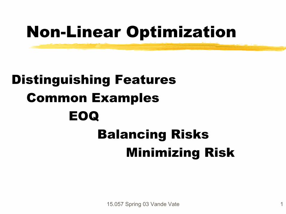
Hierarchy of Models

Network Flows

Linear Programs Mixed Integer Linear Programs



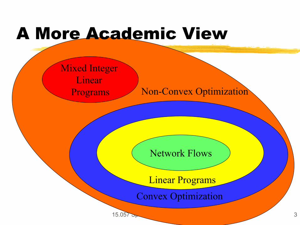
A More Academic View

Network Flows

Linear Programs Convex Optimization

Mixed Integer Linear

Programs Non-Convex Optimization


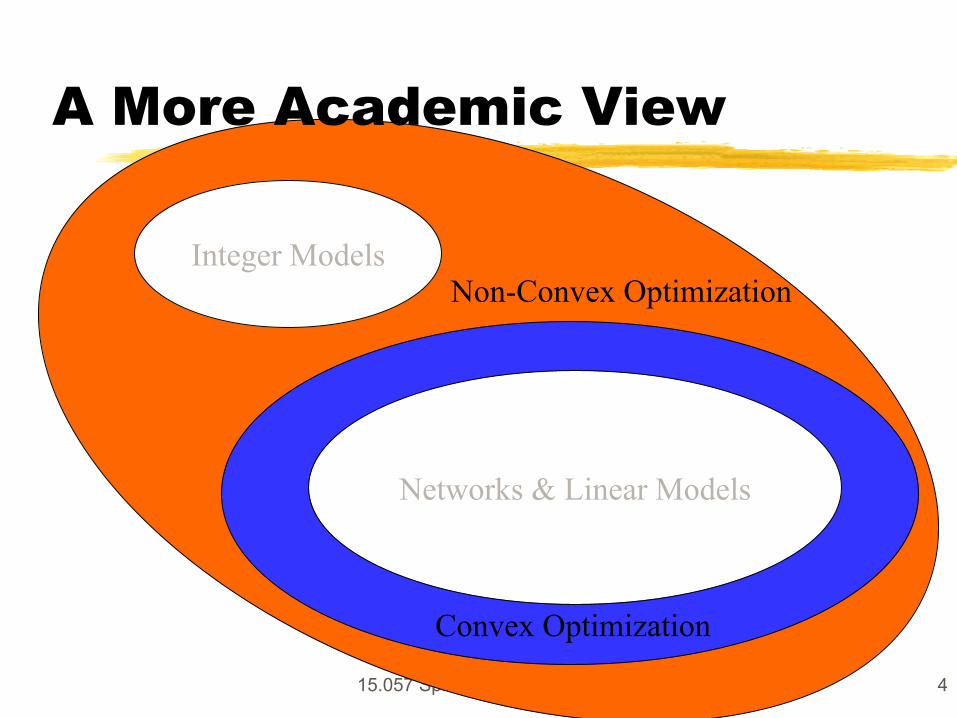
A More Academic View

Networks & Linear Models

Convex Optimization

Integer Models Non-Convex Optimization

Convexity The Distinguishing Feature

Separates Hard from Easy

Convex Combination Weighted Average

Non-negative weights Weights sum to 1


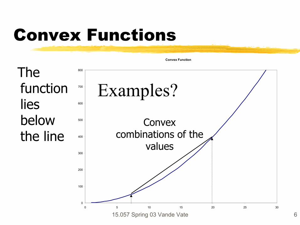
Convex Functions

The function lies below the line

Convex Function

800

700

600

500

400

300

200

100

0

Examples? Convex

combinations of the values

0 5 10 15 20 25 30


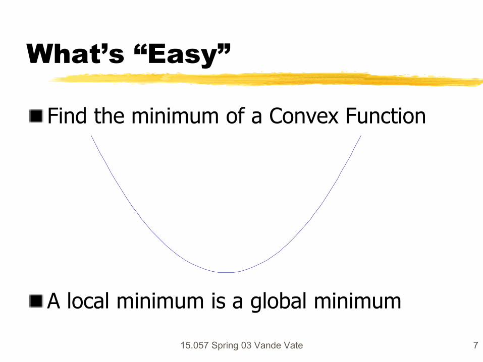
What’s “Easy”

Find the minimum of a Convex Function

A local minimum is a global minimum


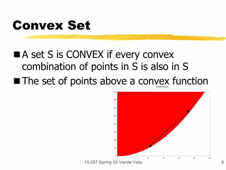
Convex Set

A set S is CONVEX if every convex combination of points in S is also in S The set of points above a convex function

Convex Function

800

700

600

500

400

300

200

100

0 0 5 10 15 20 25 30


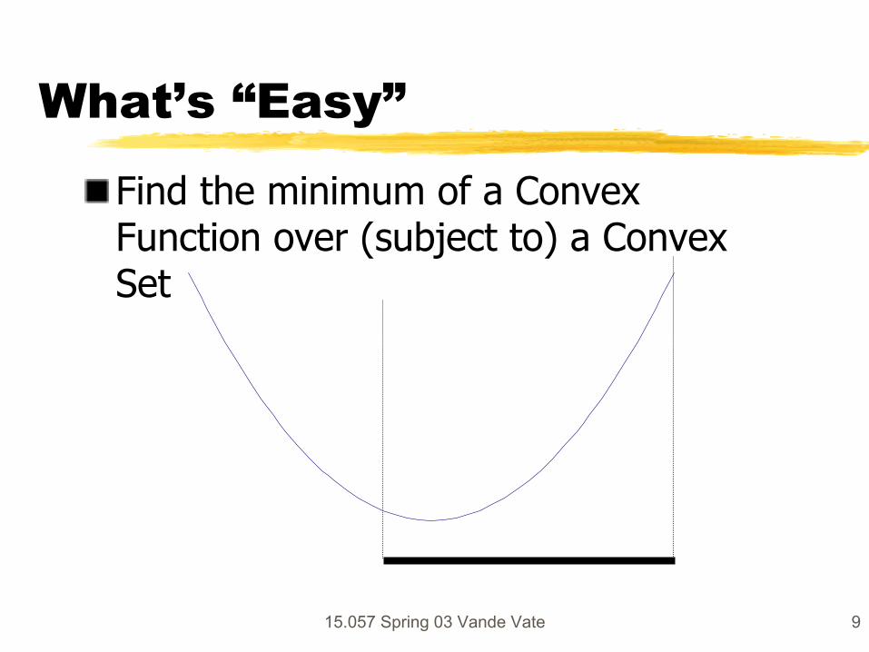
What’s “Easy”

Find the minimum of a Convex

Set Function over (subject to) a Convex


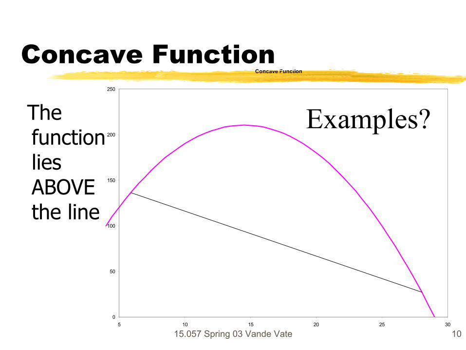
Concave Function Concave Function

The function lies ABOVE the line

0

50

100

150

200

250

Examples?

5 10 15 20 25 30


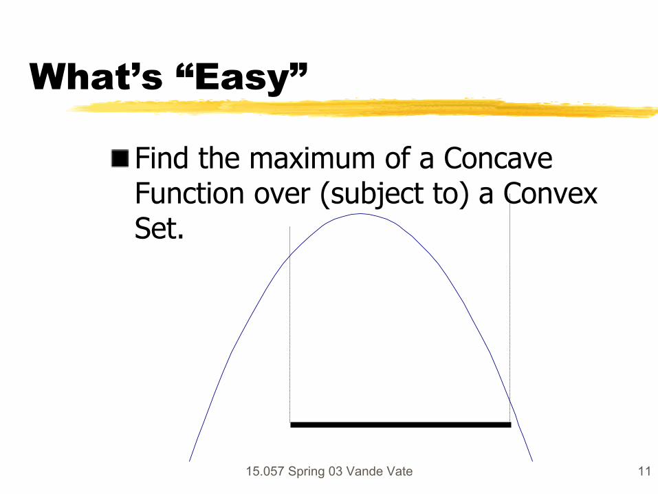
What’s “Easy”

Find the maximum of a Concave

Set. Function over (subject to) a Convex


Academic Questions

Is a linear function convex or concave? Do the feasible solutions of a linear program form a convex set?

program form a convex set?

12

Do the feasible solutions of an integer

15.057 Spring 03 Vande Vate

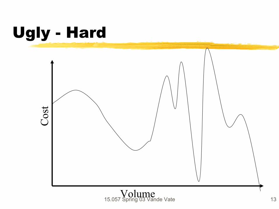
Ugly - HardC

ost

Volume15.057 Spring 03 Vande Vate 13

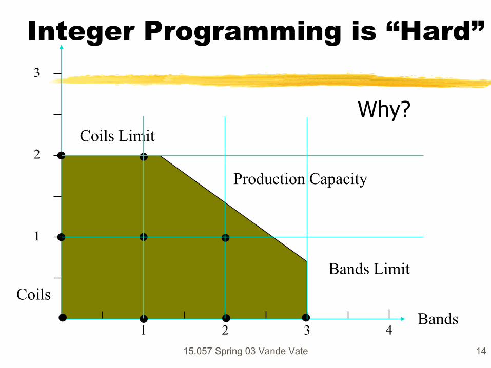
Integer Programming is “Hard”

Bands Coils

Bands Limit

Coils Limit

Production Capacity

Why?

3

2

1

1 2 3 4


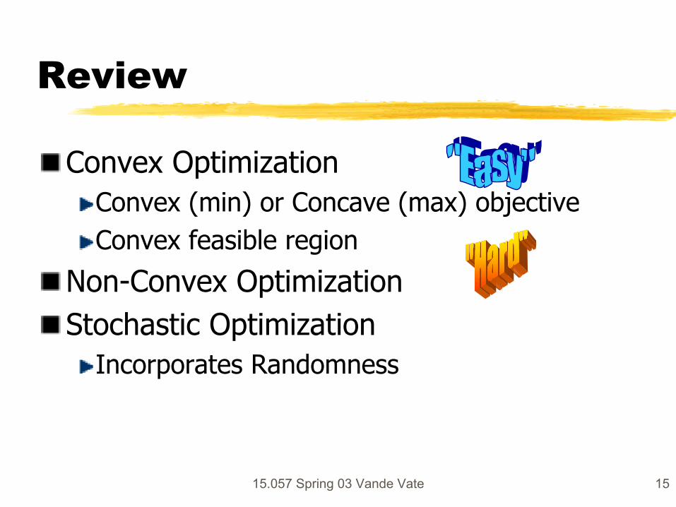
Review

Convex Optimization Convex (min) or Concave (max) objective Convex feasible region

Non-Convex Optimization Stochastic Optimization

Incorporates Randomness


Agenda

Convex Optimization Unconstrained Optimization Constrained Optimization

Non-Convex Optimization Convexification Heuristics


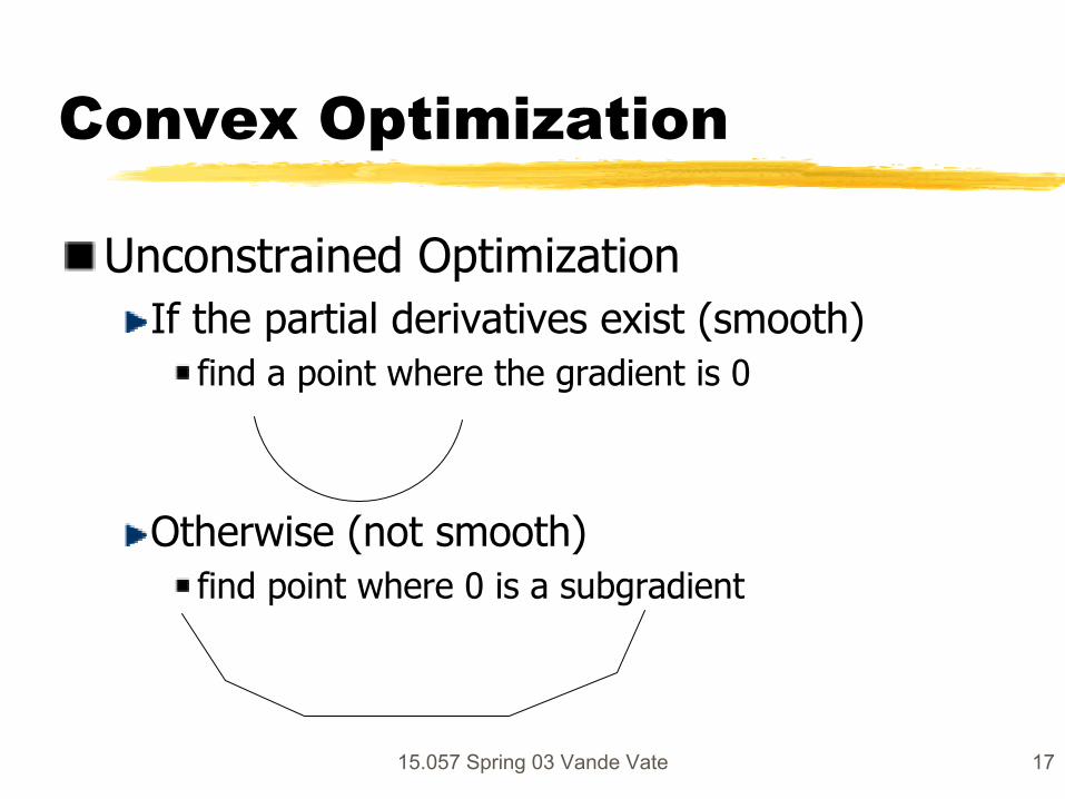
Convex Optimization

Unconstrained Optimization If the partial derivatives exist (smooth)

find a point where the gradient is 0

Otherwise (not smooth) find point where 0 is a subgradient


Unconstrained Convex Optimization

Smooth Find a point where the Gradient is 0 Find a solution to ∇f(x) = 0

Analytically (when possible) Iteratively otherwise


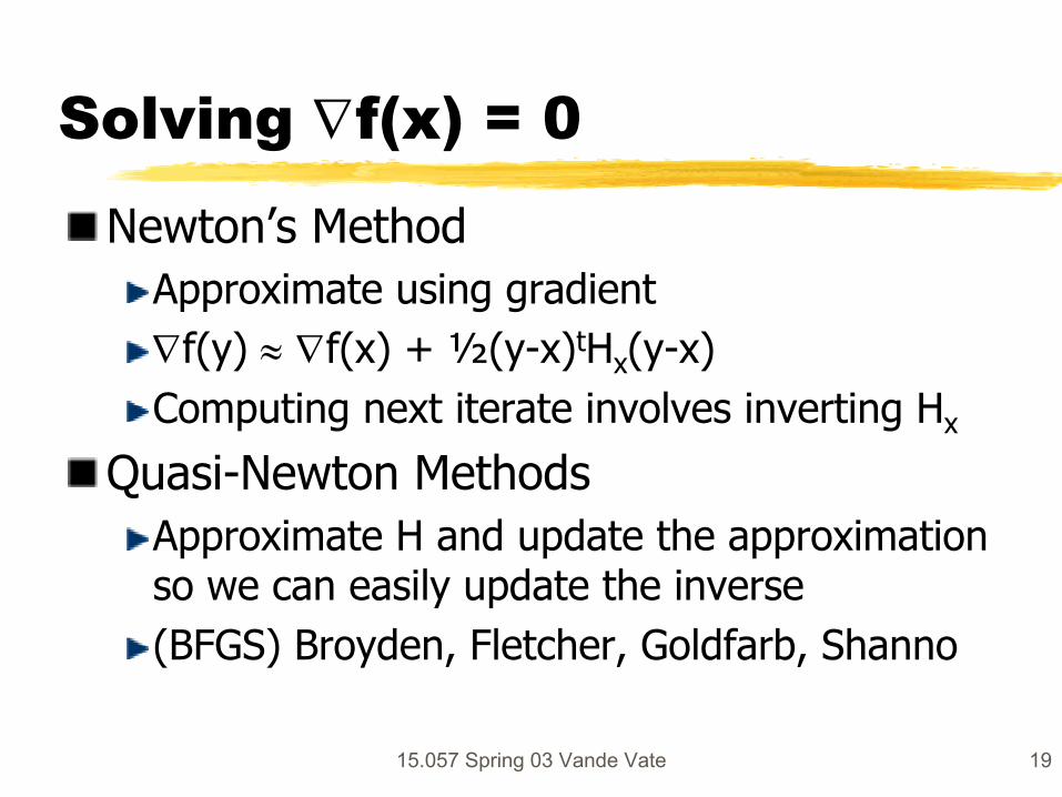
Solving ∇f(x) = 0

Newton’s Method Approximate using gradient ∇f(y) ≈ ∇f(x) + ½(y-x)tHx(y-x) Computing next iterate involves inverting Hx

Quasi-Newton Methods Approximate H and update the approximation so we can easily update the inverse (BFGS) Broyden, Fletcher, Goldfarb, Shanno


Line Search

Newton/Quasi-Newton Methods yield direction to next iterate 1-dimensional search in this direction

Several methods


Unconstrained Convex Optimization

Non-smooth Subgradient Optimization Find a point where 0 is a subgradient



What’s a Subgradient

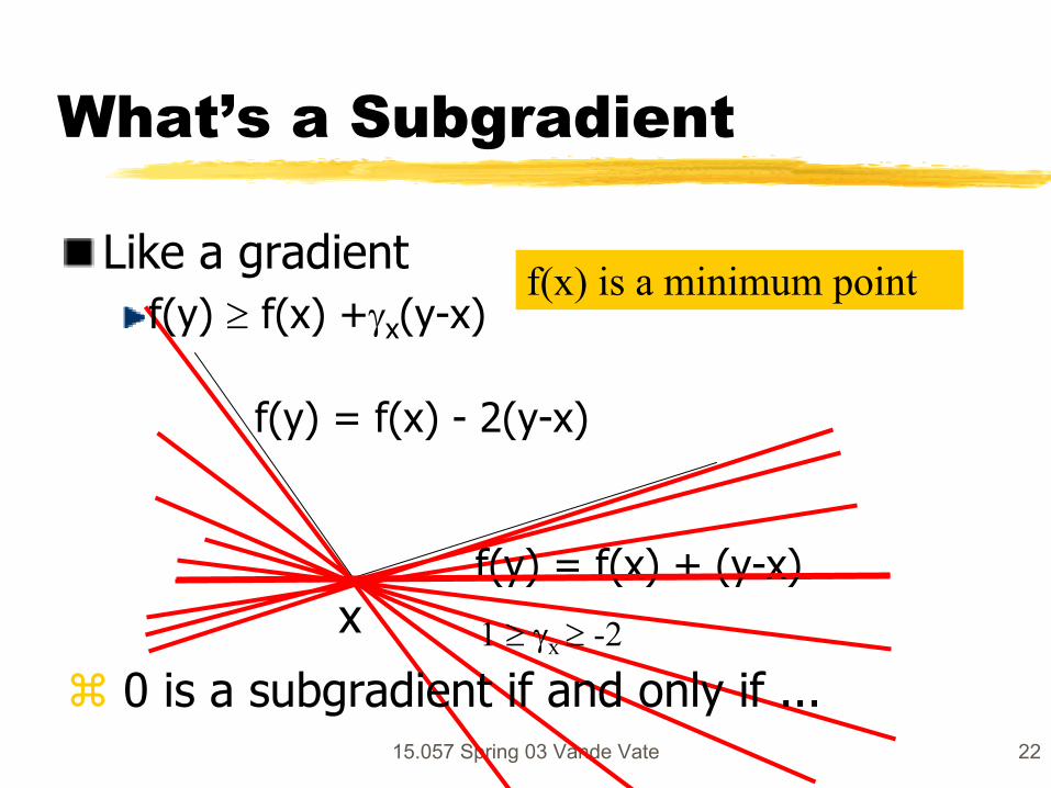
f(y) = f(x) - 2(y-x)

x

a 0 is a subgradient if and only if ... 1 ≥ γx ≥ -2

f(y) = f(x) + (y-x)

Like a gradient f(y) ≥ f(x) +γx(y-x)

f(x) is a minimum point

Steepest Descent

If 0 is not a subgradient at x, subgradient indicates where to go

Direction of steepest descent

Find the best point in that direction line search


Examples

EOQ Model Balancing Risk Minimizing Risk


EOQ

How large should each order be

Trade-off Cost of Inventory (known) Cost of transactions (what?)

Larger orders Higher Inventory Cost Lower Ordering Costs


The Idea

Increase the order size until the incremental cost of holding the last item equals the incremental savings in ordering costs If the costs exceed the savings? If the savings exceed the costs?


Modeling Costs Q is the order quantity Average inventory level is

Q/2 h*c is the Inv. Cost. in $/unit/year Total Inventory Cost

h*c*Q/2 Last item contributes what to inventory cost?

h*c/2


Modeling Costs D is the annual demand How many orders do we place?

D/Q

Transaction cost is A per transaction Total Transaction Cost

AD/Q


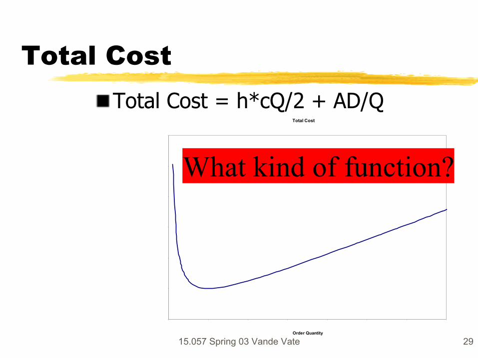
Total Cost Total Cost = h*cQ/2 + AD/Q

Total Cost

120

100

80

60

40

20

What kind of function?

0 0 10 20 30 40 50 60 70

Order Quantity


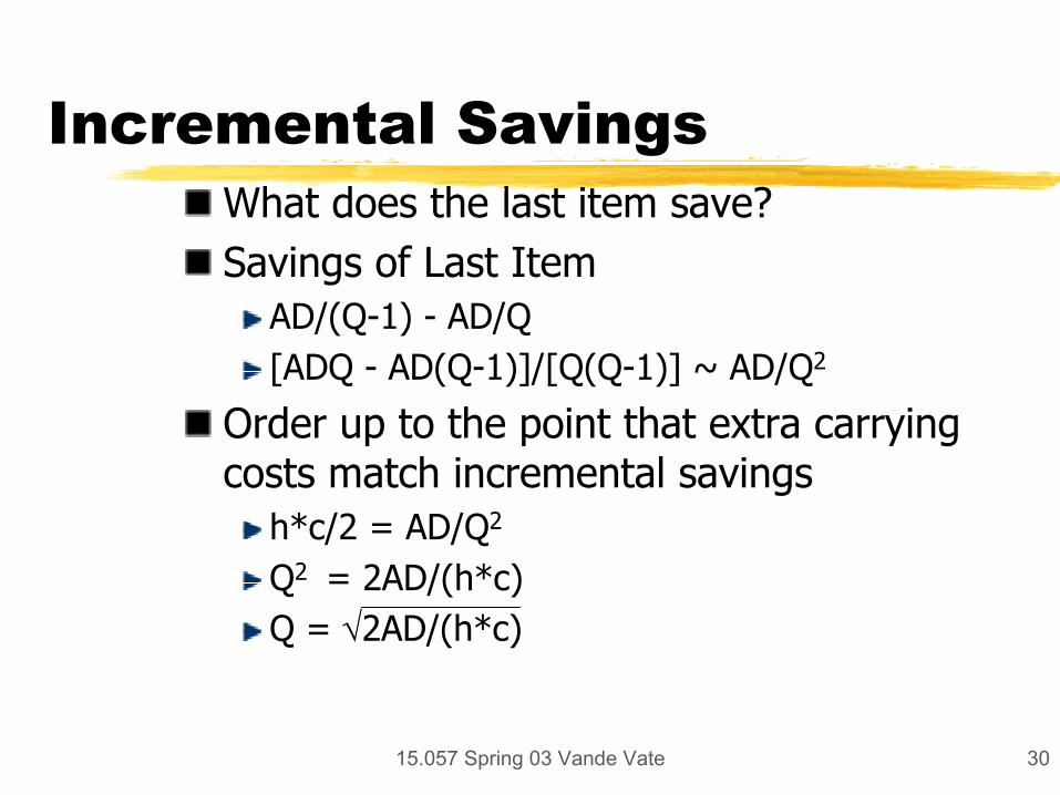
Incremental Savings What does the last item save? Savings of Last Item

AD/(Q-1) - AD/Q [ADQ - AD(Q-1)]/[Q(Q-1)] ~ AD/Q2

Order up to the point that extra carrying costs match incremental savings

h*c/2 = AD/Q2

Q2 = 2AD/(h*c) Q = √2AD/(h*c)


Key Assumptions?

Known constant rate of demand


Value?

No one can agree on the ordering costEach value of the ordering cost implies

A value of Q from which we get An inventory investment c*Q/2 A number of orders per year: D/Q

Trace the balance for each value of ordering costs


The EOQ Trade offKnown values

Annual Demand D Product value c Inventory carrying percentage h

Unknown transaction cost A For each value of A

Calculate Q = √2AD/(h*c) Calculate Inventory Investment cQ/2 Calculate Annual Orders D/Q


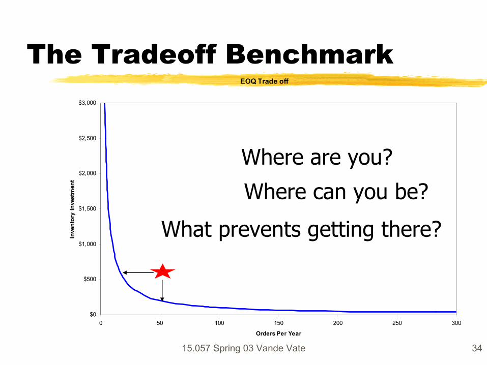
The Tradeoff BenchmarkEOQ Trade off

$3,000

$2,500

$2,000

$1,500

$1,000

$500

Inve

ntor

y In

vest

men

t

Where are you?

Where can you be?

But wait…!What prevents getting there?

$0 0 50 100 150 200 250 300

Orders Per Year


Balancing Risks


Variability Some events are inherently variable

When customers arriveHow many customers arriveTransit timesDaily usage Stock Prices...

Hard to predict exactly Dice Lotteries


Random Variables Examples

Outcome of rolling a dice Closing Stock price Daily usage Time between customer arrivals Transit time Seasonal Demand


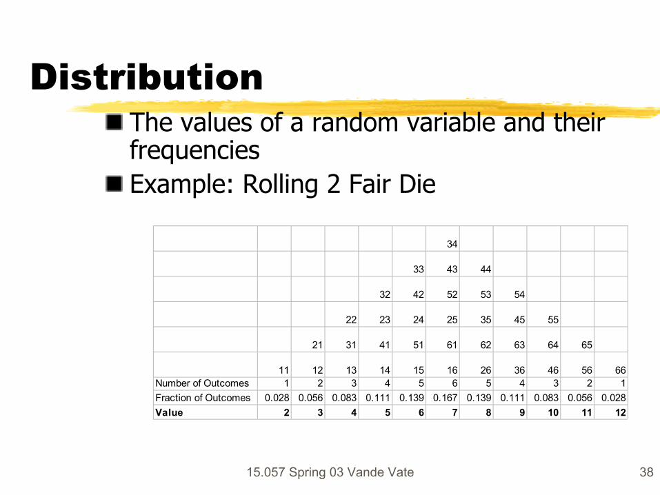
Distribution The values of a random variable and their frequencies Example: Rolling 2 Fair Die

34

33 43 44

32 42 52 53 54

22 23 24 25 35 45 55

21 31 41 51 61 62 63 64 65

11 12 13 14 15 16 26 36 46 56 66 Number of Outcomes 1 2 3 4 5 6 5 4 3 2 1 Fraction of Outcomes 0.028 0.056 0.083 0.111 0.139 0.167 0.139 0.111 0.083 0.056 0.028 Value 2 3 4 5 6 7 8 9 10 11 12


Theoretical vs Empirical

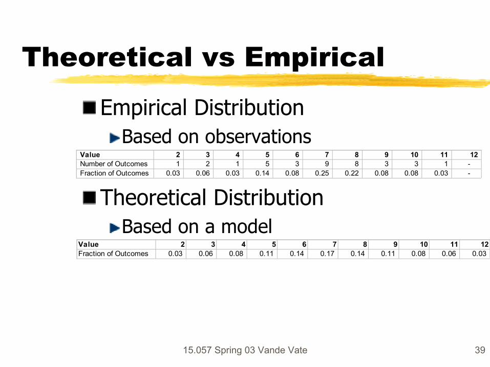
Empirical Distribution Based on observations

Value 2 3 4 5 6 7 8 9 10 11 12 Number of Outcomes 1 2 1 5 3 9 8 3 3 1 -Fraction of Outcomes 0.03 0.06 0.03 0.14 0.08 0.25 0.22 0.08 0.08 0.03 -

Theoretical Distribution Based on a model

Value 2 3 4 5 6 7 8 9 10 11 12 Fraction of Outcomes 0.03 0.06 0.08 0.11 0.14 0.17 0.14 0.11 0.08 0.06 0.03


Empirical vs Theoretical

One Perspective: If the die are fair and we roll many many times, empirical should match theoretical. Another Perspective: If the die are reasonably fair, the theoretical is close and saves the trouble of rolling.


Empirical vs Theoretical The Empirical Distribution is flawed because it relies on limited observations The Theoretical Distribution is flawed because it necessarily ignores details about reality Exactitude? It’s random.


Continuous vs Discrete

Discrete Value of dice Number of units sold …

Continuous Essentially, if we measure it, it’s discrete Theoretical convenience


Probability Discrete: What’s the probability we roll a 12 with two fair die:

1/36 Continuous: What’s the probability the temperature will be exactly 72.00o F tomorrow at noon EST?

Zero! Events: What’s the probability that the temperature will be at least 72o F tomorrow at noon EST?


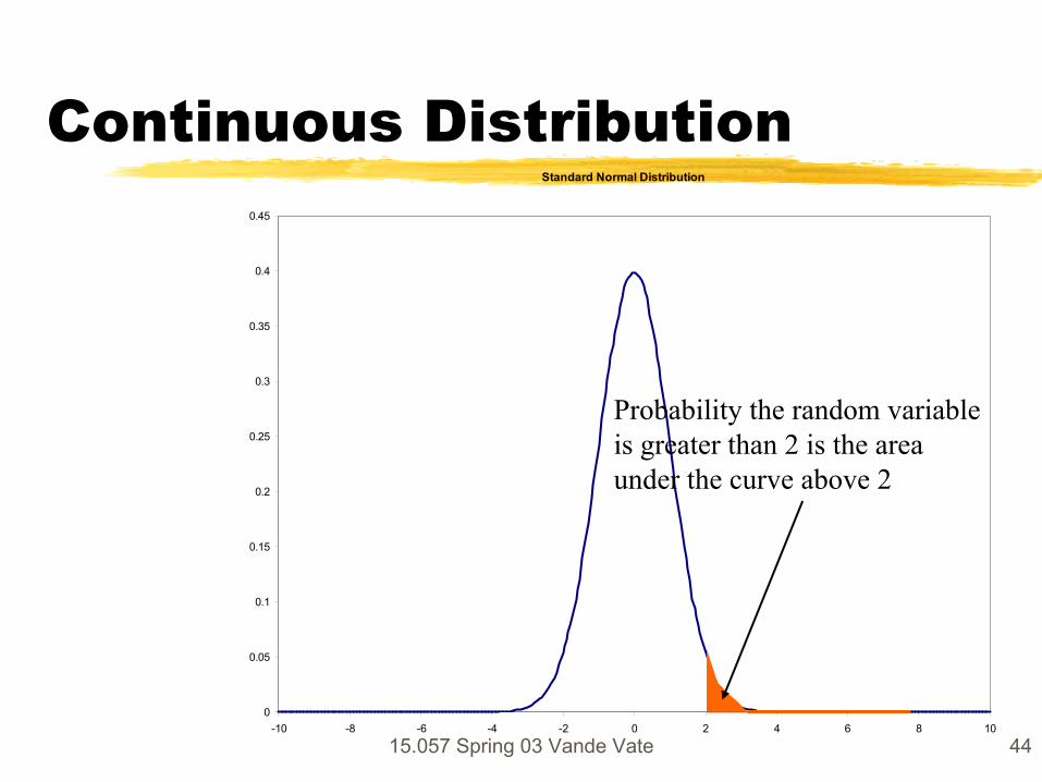
Continuous Distribution Standard Normal Distribution

0.45

0.4

0.35

0.3

0.25

0.2

0.15

0.1

0.05

Probability the random variable is greater than 2 is the area under the curve above 2

0 -10 -8 -6 -4 -2 0 2 4 6 8 10


Total Probability Empirical, Theoretical, Continuous, Discrete, … Probability is between 0 and 1

Total Probability (over all possible outcomes) is 1


Summary Stats The Mean

Weights each outcome by its probability AKA

Expected Value Average

May not even be possible Example:

Win $1 on Heads, nothing on Tails


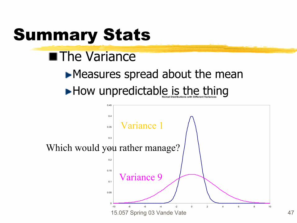
Summary Stats The Variance

Measures spread about the mean How unpredictable is the thing

Nomal Distributions with Different Variances

0.45

0.4

0.35

0.3

0.25Which would you rather manage? 0.2

0.15

0.1

Variance 1

Variance 9 0.05

0 -10 -8 -6 -4 -2 0 2 4 6 8 10


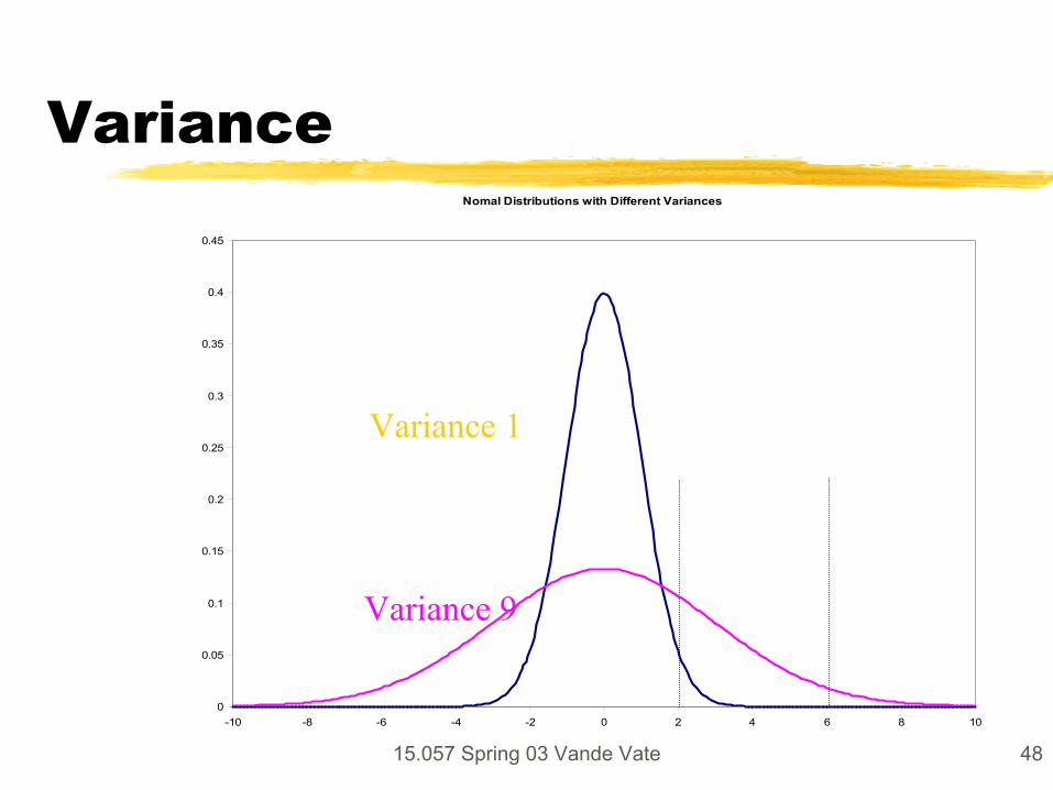
Variance Nomal Distributions with Different Variances

0.45

0.4

0.35

0.3

0.25

0.2

0.15

0.1

0.05

Variance 1

Variance 9

0 -10 -8 -6 -4 -2 0 2 4 6 8 10


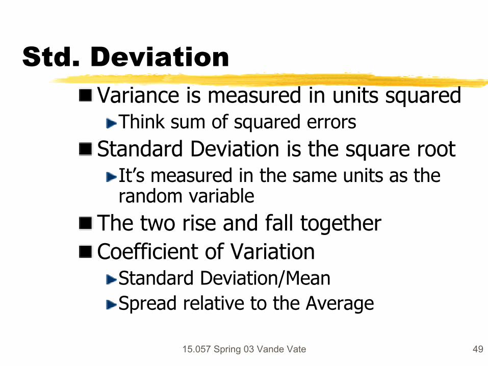
Std. DeviationVariance is measured in units squared

Think sum of squared errors Standard Deviation is the square root

It’s measured in the same units as the random variable

The two rise and fall together Coefficient of Variation

Standard Deviation/Mean Spread relative to the Average


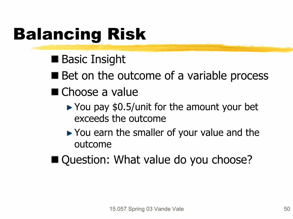
Balancing Risk Basic Insight Bet on the outcome of a variable process Choose a value

You pay $0.5/unit for the amount your bet exceeds the outcome You earn the smaller of your value and the outcome

Question: What value do you choose?


Similar to...

Anything you are familiar with?


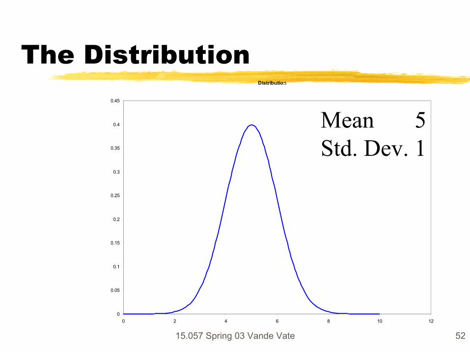
The DistributionDistribution

0.45

0.4

0.35

0.3

0.25

0.2

0.15

0.1

0.05

Mean Std. Dev. 1

5

0 0 2 4 6 8 10 12


The Idea

Balance the risks Look at the last item

What did it promise? What risk did it pose?

If Promise is greater than the risk?

If the Risk is greater than the promise?


Measuring Risk and Return Revenue from the last item

$1 if the Outcome is greater,$0 otherwise

Expected Revenue $1*Probability Outcome is greater than our choice

Risk posed by last item $0.5 if the Outcome is smaller, $0 otherwise

Expected Risk $0.5*Probability Outcome is smaller than our choice


Balancing Risk and Reward Expected Revenue

$1*Probability Outcome is greater than our choice


How are probabilities Related?


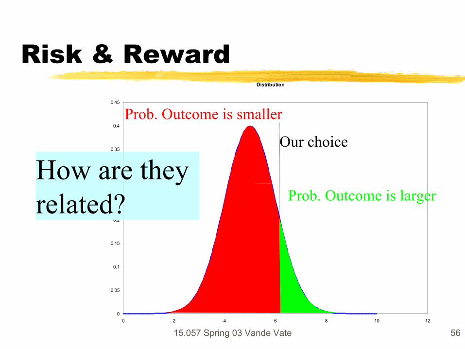
Risk & RewardDistribution

0

0.05

0.1

0.15

0.2

0.35

0.4

0.45

Prob. Outcome is smaller

Prob. Outcome is larger

Our choice

How are they related?

0 2 4 6 8 10 12


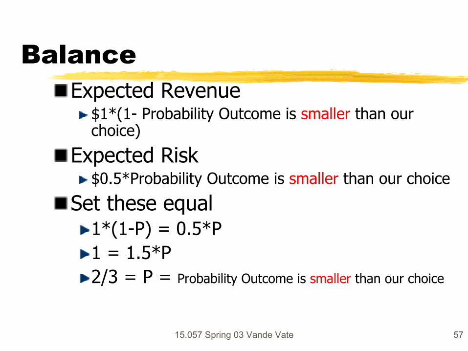
BalanceExpected Revenue

$1*(1- Probability Outcome is smaller than our choice)


Set these equal 1*(1-P) = 0.5*P1 = 1.5*P2/3 = P = Probability Outcome is smaller than our choice


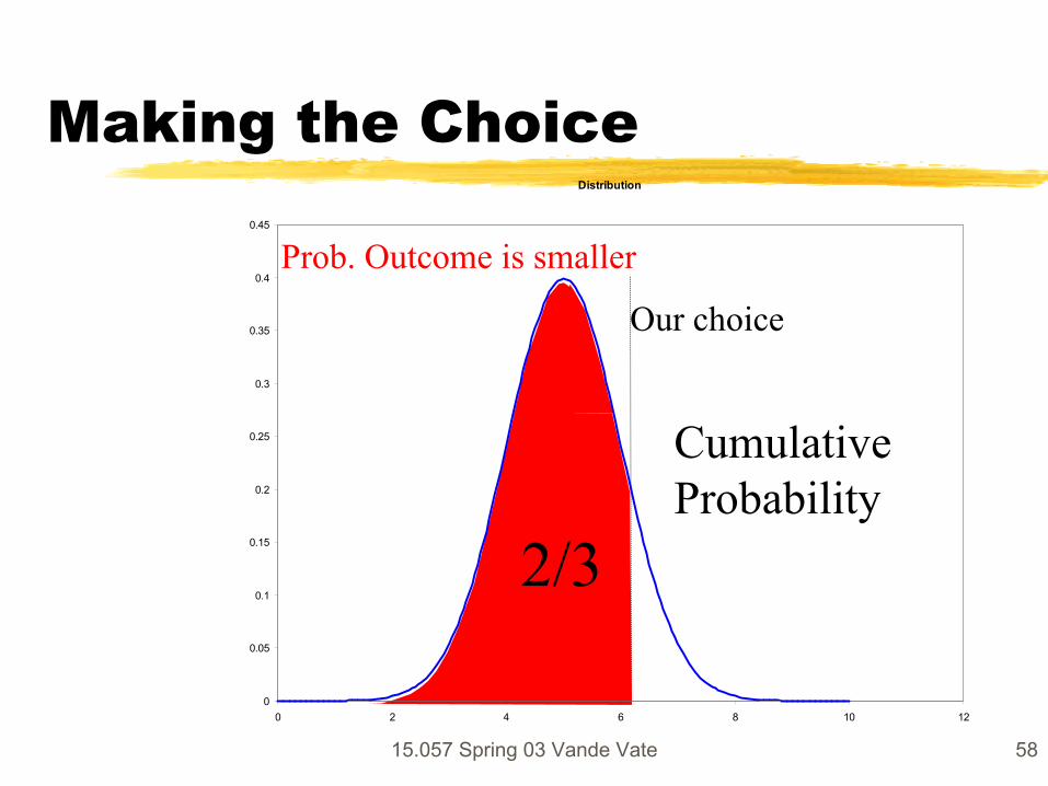
Making the Choice Distribution

0.45

0.4

0.35

0.3

0.25

0.2

0.15

0.1

0.05

Prob. Outcome is smaller

Our choice

2/3

Cumulative Probability

0 0 2 4 6 8 10 12


Constrained Optimization

Feasible Direction techniques

Eliminating constraints Implicit Function Penalty Methods

Duality


Feasible Directions

Unconstrained OptimizationX Start at a point: x0

Identify an^ improving direction: dFeasible

Find a best ^ solution in direction d: x + εd FeasibleRepeat

A Feasible direction: one you can move inA Feasible solution: don’t move too far. Typically for Convex feasible region


Constrained Optimization

Penalty Methods Move constraints to objective with penalties or barriers

As solution approaches the constraint the penalty increases Example:

min f(x) => min f(x) + t/(3x - x2) s.t. x2 ≤ 3x

as x2 approaches 3x, penalty increases rapidly


Relatively reliable tools for

Quadratic objective Linear constraints Continuous variables


Summary “Easy Problems”

Convex Minimization Concave Maximization

Unconstrained Optimization Local gradient information

Constrained problems Tricks for reducing to unconstrained or simply constrained problems

NLP tools practical only for “smaller” problems


Documents

Distinguishing Features Common Examples EOQ … · 400 300 200 100 0 0 5 10 15 20 25 30 15.057 Spring 03 Vande Vate 8 . ... Standard Deviation is the square root It’s measured in