Embed Size (px)
Citation preview
Aalborg University
Master Thesis - Electronics & IT- Signal Processing and Computing
Distant Speech Recognition
Author:Nicolai B. Thomsen
Supervisors:Zheng-Hua Tan (AAU)
Søren Holdt Jensen (AAU)John H.L. Hansen (UTD)
June 6, 2013

Department of Electronic SystemsElectronics & ITFredrik Bajers Vej 7 B9220 Aalborg ØPhone 9940 8600http://es.aau.dk
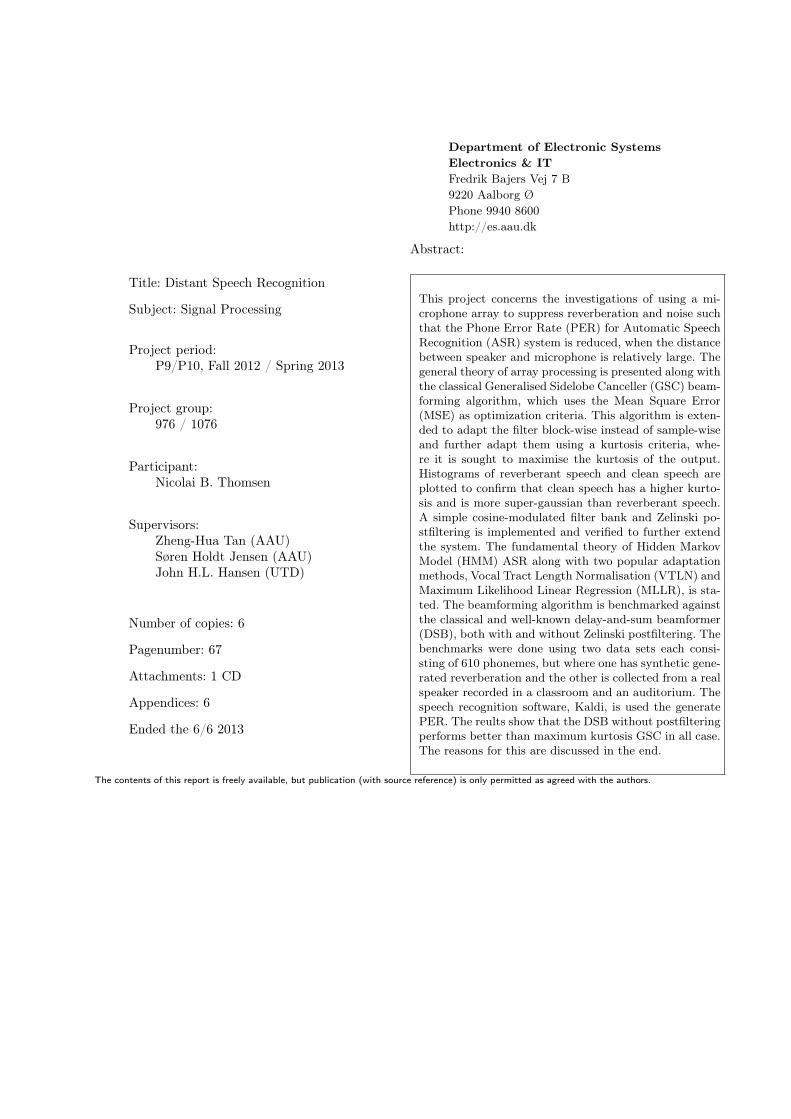
Title: Distant Speech Recognition
Subject: Signal Processing
Project period:P9/P10, Fall 2012 / Spring 2013
Project group:976 / 1076
Participant:Nicolai B. Thomsen
Supervisors:Zheng-Hua Tan (AAU)Søren Holdt Jensen (AAU)John H.L. Hansen (UTD)
Number of copies: 6
Pagenumber: 67
Attachments: 1 CD
Appendices: 6
Ended the 6/6 2013
Abstract:
This project concerns the investigations of using a mi-crophone array to suppress reverberation and noise suchthat the Phone Error Rate (PER) for Automatic SpeechRecognition (ASR) system is reduced, when the distancebetween speaker and microphone is relatively large. Thegeneral theory of array processing is presented along withthe classical Generalised Sidelobe Canceller (GSC) beam-forming algorithm, which uses the Mean Square Error(MSE) as optimization criteria. This algorithm is exten-ded to adapt the filter block-wise instead of sample-wiseand further adapt them using a kurtosis criteria, whe-re it is sought to maximise the kurtosis of the output.Histograms of reverberant speech and clean speech areplotted to confirm that clean speech has a higher kurto-sis and is more super-gaussian than reverberant speech.A simple cosine-modulated filter bank and Zelinski po-stfiltering is implemented and verified to further extendthe system. The fundamental theory of Hidden MarkovModel (HMM) ASR along with two popular adaptationmethods, Vocal Tract Length Normalisation (VTLN) andMaximum Likelihood Linear Regression (MLLR), is sta-ted. The beamforming algorithm is benchmarked againstthe classical and well-known delay-and-sum beamformer(DSB), both with and without Zelinski postfiltering. Thebenchmarks were done using two data sets each consi-sting of 610 phonemes, but where one has synthetic gene-rated reverberation and the other is collected from a realspeaker recorded in a classroom and an auditorium. Thespeech recognition software, Kaldi, is used the generatePER. The reults show that the DSB without postfilteringperforms better than maximum kurtosis GSC in all case.The reasons for this are discussed in the end.
The contents of this report is freely available, but publication (with source reference) is only permitted as agreed with the authors.

Institut for Elektroniske SystemerElektronik og ITFredrik Bajers Vej 7 B9220 Aalborg ØTelefon 9940 8600http://es.aau.dk
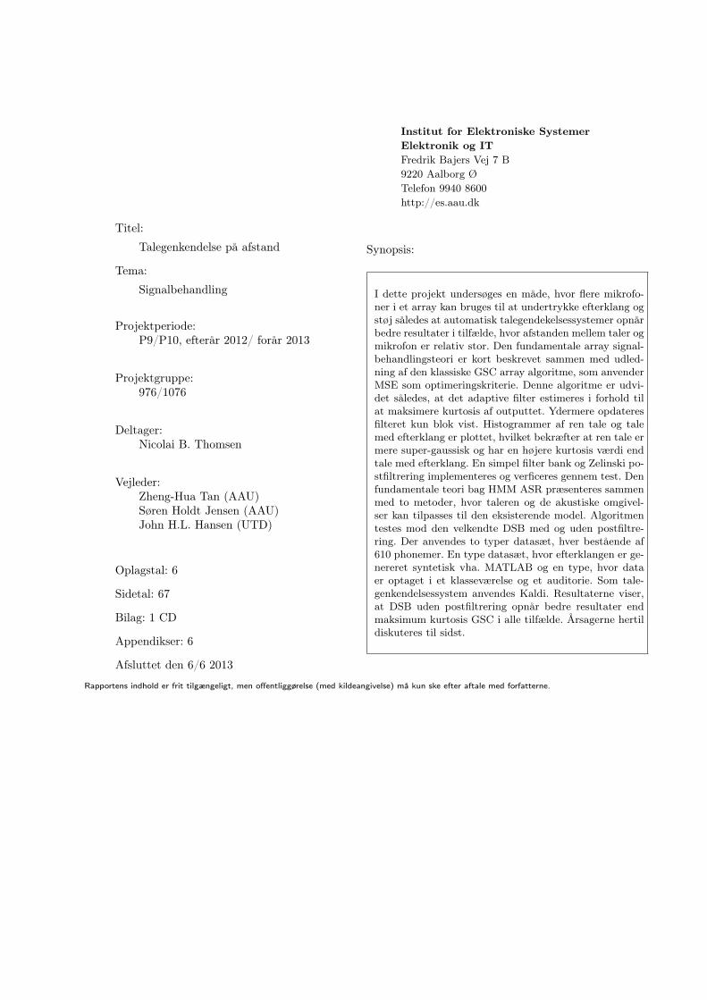
Titel:
Talegenkendelse på afstand
Tema:
Signalbehandling
Projektperiode:P9/P10, efterår 2012/ forår 2013
Projektgruppe:976/1076
Deltager:Nicolai B. Thomsen
Vejleder:Zheng-Hua Tan (AAU)Søren Holdt Jensen (AAU)John H.L. Hansen (UTD)
Oplagstal: 6
Sidetal: 67
Bilag: 1 CD
Appendikser: 6
Afsluttet den 6/6 2013
Synopsis:
I dette projekt undersøges en måde, hvor flere mikrofo-ner i et array kan bruges til at undertrykke efterklang ogstøj således at automatisk talegendekelsessystemer opnårbedre resultater i tilfælde, hvor afstanden mellem taler ogmikrofon er relativ stor. Den fundamentale array signal-behandlingsteori er kort beskrevet sammen med udled-ning af den klassiske GSC array algoritme, som anvenderMSE som optimeringskriterie. Denne algoritme er udvi-det således, at det adaptive filter estimeres i forhold tilat maksimere kurtosis af outputtet. Ydermere opdateresfilteret kun blok vist. Histogrammer af ren tale og talemed efterklang er plottet, hvilket bekræfter at ren tale ermere super-gaussisk og har en højere kurtosis værdi endtale med efterklang. En simpel filter bank og Zelinski po-stfiltrering implementeres og verficeres gennem test. Denfundamentale teori bag HMM ASR præsenteres sammenmed to metoder, hvor taleren og de akustiske omgivel-ser kan tilpasses til den eksisterende model. Algoritmentestes mod den velkendte DSB med og uden postfiltre-ring. Der anvendes to typer datasæt, hver bestående af610 phonemer. En type datasæt, hvor efterklangen er ge-nereret syntetisk vha. MATLAB og en type, hvor dataer optaget i et klasseværelse og et auditorie. Som tale-genkendelsessystem anvendes Kaldi. Resultaterne viser,at DSB uden postfiltrering opnår bedre resultater endmaksimum kurtosis GSC i alle tilfælde. Årsagerne hertildiskuteres til sidst.
Rapportens indhold er frit tilgængeligt, men offentliggørelse (med kildeangivelse) må kun ske efter aftale med forfatterne.

Preface
This report has been made by Nicolai Bæk Thomsen in the period September 2012 to June 2013as documentation of Master Thesis in Signal Processing and Computing at the Department ofElectronic Systems, Aalborg University. From ultimo January to medio April I was a visitingstudent at Center for Robust Speech Systems (CRSS) at UT Dallas, Texas, under the supervisionof Professor Dr. John H.L. Hansen. This stay was among other spent on setting up an AutomaticSpeech Recognition (ASR) system and collecting real-world data. I would like to thank everybodyat CRSS for making the stay a succes through fruitful debates and discussions within the field ofsignal processing. A special thanks to Professor Dr. Hansen for letting me visit and for helpingme collect data. Thanks to Dr. Seong-Jun Hahm the CRSS for valuable help on setting up theASR system. All code is written in MATLAB and can be found on the supplied CD. The Kaldisoftware used to do speech recognition is not supplied on the CD but can be found at http://kaldi.sourceforge.net/index.html.
Reading guide
Matrices are written in bold with capital letters (A), and vectors are just written in bold (a).Notation, which is not standardized, is explained at first encounter. All relevant equations arenumbered. The first time acronyms are used the full word/sentence is stated, and furthermore alist of acronyms is provided. The content of the report is organised in the following way: Chapter 1gives a soft introduction to the application of speech recognition and the motivation for improvingthe performance when the distance between speaker and microphone is increased. Chapter 2 statesthe reverberant signal model and the statistic properties of the signals involved. Chapter 3 givesan overview of array processing and derives the classic Generalised Sidelobe Canceller (GSC) andextends the algorithm using a kurtosis criteria. Chapter 4 gives a brief overview of the theorybehind ASR and chapter 5 states and discuss the results achieved. Finally, chapter 6 concludes onthe thesis and discusses how to proceed. Appendices are found at the back of the report.
Nicolai B. Thomsen - Aalborg 6/6, 2013
vii
Indhold
1 Introduction 1
2 Problem Description 22.1 Signal model in acoustic environment . . . . . . . . . . . . . . . . . . . . . . . . . . 22.2 Objective of speech enhancement . . . . . . . . . . . . . . . . . . . . . . . . . . . . 3
3 Array Signal Processing 53.1 Array response and signal model . . . . . . . . . . . . . . . . . . . . . . . . . . . . 53.2 Generalised Sidelobe Canceller (GSC) . . . . . . . . . . . . . . . . . . . . . . . . . 63.3 Maximum Kurtosis Subband GSC . . . . . . . . . . . . . . . . . . . . . . . . . . . 143.4 Summary . . . . . . . . . . . . . . . . . . . . . . . . . . . . . . . . . . . . . . . . . 32
4 Speech Recognition 334.1 HMM and GMM . . . . . . . . . . . . . . . . . . . . . . . . . . . . . . . . . . . . . 334.2 Features . . . . . . . . . . . . . . . . . . . . . . . . . . . . . . . . . . . . . . . . . . 354.3 Adaptation . . . . . . . . . . . . . . . . . . . . . . . . . . . . . . . . . . . . . . . . 354.4 Kaldi . . . . . . . . . . . . . . . . . . . . . . . . . . . . . . . . . . . . . . . . . . . . 37
5 Experimental Results 385.1 Data . . . . . . . . . . . . . . . . . . . . . . . . . . . . . . . . . . . . . . . . . . . . 385.2 Results . . . . . . . . . . . . . . . . . . . . . . . . . . . . . . . . . . . . . . . . . . . 385.3 Discussion . . . . . . . . . . . . . . . . . . . . . . . . . . . . . . . . . . . . . . . . . 44
6 Conclusion 45
References 47
Appendix 49A Deriving the Linear Constrained Minimum-Variance optimum filter . . . . . . . . . 51B Derivation of the sample kurtosis gradient . . . . . . . . . . . . . . . . . . . . . . . 52C Kurtosis of random variable with standard normal distribution . . . . . . . . . . . 54D Estimated kurtosis for individual phonemes . . . . . . . . . . . . . . . . . . . . . . 55E TIMIT sentences . . . . . . . . . . . . . . . . . . . . . . . . . . . . . . . . . . . . . 56F Overview of rooms used for recording . . . . . . . . . . . . . . . . . . . . . . . . . . 57
viii
Acronyms
AIR Acoustic Impulse Response. 3, 4
ASR Automatic Speech Recognition. iii, v, vii, 2, 3, 32, 33, 35–39, 44
AWGN Additive White Gaussian Noise. 3, 25, 26
CLT Central Limit Theorem. 19, 45
cMLLR constrained Maximum Likelihood Linear Regression. 36
DFT Discrete Fourier Transform. 28, 35
DOA Direction-of-Arrival. 14
DOI Direction-Of-Interest. 12, 31
DSB delay-and-sum beamformer. iii, v, 38, 39, 42–45
DSR Distant Speech Recognition. 1
EVD Eigenvalue Decomposition. 25
GMM Gaussian Mixture Model. 33, 35, 37
GSC Generalised Sidelobe Canceller. iii, v, vii, 1, 7, 12–14, 16, 19, 21, 26, 30, 32, 37–39, 41–45
HMM Hidden Markov Model. iii, v, 33–38, 45
iDFT Inverse Discrete Fourier Transform. 35
MFCC Mel-Frequency Cepstrum Coefficient. 35–37
MLLR Maximum Likelihood Linear Regression. iii, 37, 39, 42, 45
MSE Mean Square Error. iii, v, 18, 27, 32
NLMS Normalised Least-Mean-Square. 9
PDF Probability Density Function. 19, 34, 54
PER Phone Error Rate. iii, 1, 3, 33, 38, 39, 41, 43, 45
PSD Power Spectral Density. 27–29
RIR Room Impulse Response. 38
ix

SNIR signal-to-noise plus interference ratio. 29
SNR signal-to-noise ratio. 29, 30, 32, 39
SOI Signal-Of-Interest. 12–14
ULA Uniform Linear Array. 5, 14, 32, 44
VTLN Vocal Tract Length Normalisation. iii, 37, 39, 42, 45
WER Word Error Rate. 3
WSS Wide Sense Stationary. 26, 27
x
Kapitel 1
Introduction
It is becoming more and more popular for people to use some kind of computer/device (smartphone,tablet, PC etc.) on a daily basis. The interaction is primarily done using some kind of touch input,which is not very practical since it ties the user’s hands to the device or perhaps the user is not ableto use his/her hands. A typical scenario of the first case could be when driving a car, in which casethe user has to use his/her hands to operate the steering wheel and the gear stick [1]. An exampleof the second case is disabled people who simply cannot operate their hands at the required levelof precision. In such cases it is desirable to be able to interact with the device without the use ofhands or physical contact with the device. One method which is becoming more and more popularis the use of voice and speech, where the device is able to understand simple commands or wholesentences. Under ideal situations where the user is close to the microphone talking directly intoit in a low-noise environment, performance is acceptable. This can be achieved by using a user-mounted microphone, but at the price of inconvenience, which is acceptable in some applicationsand situations, but as an example thi is not acceptable in multi-user settings. When the distancebetween the user and device/microphone is increased (Distant Speech Recognition (DSR)), theperformance is seriously degraded due to background noise and echo or reverberation [1]. Theseproblems have to be overcome in order for speech interaction between human and computer tobecome popular and effective, thus a lot of research has been done within the field of DSR. Oneparticular and interesting method of combating these problems is through the use of multiplemicrophones, also known as microphone array processing or beamforming. This introduces thepossibility to direct the gain towards the user and thereby supressing other sources. The scope ofthis thesis is to investigate one recent proposed method [2] and evaluate it in terms PER. Theoutline is as follows: first the problem is described along with a signal model, next a brief overviewof basic array processing theory is given along with the derivation and implementation of a classicbeamformer called GSC. After this the algorithm is extended according to [2] and evaluated interms of recognition performance. At last a conclusion on the results is made.
1
Chapter 2. Problem Description
Kapitel 2
Problem Description
The aim of this section is to describe the phenomenon of reverberation and why this poses aproblem. Based on this a reverberant signal model will be given and mainly the statistical propertiesof these signals will be stated. This will set the stage for all further investigation in this report.This section will also explain how the enhancement/dereverberation is assessed in this report, sincethere are many different ways of measuring this.
2.1 Signal model in acoustic environment
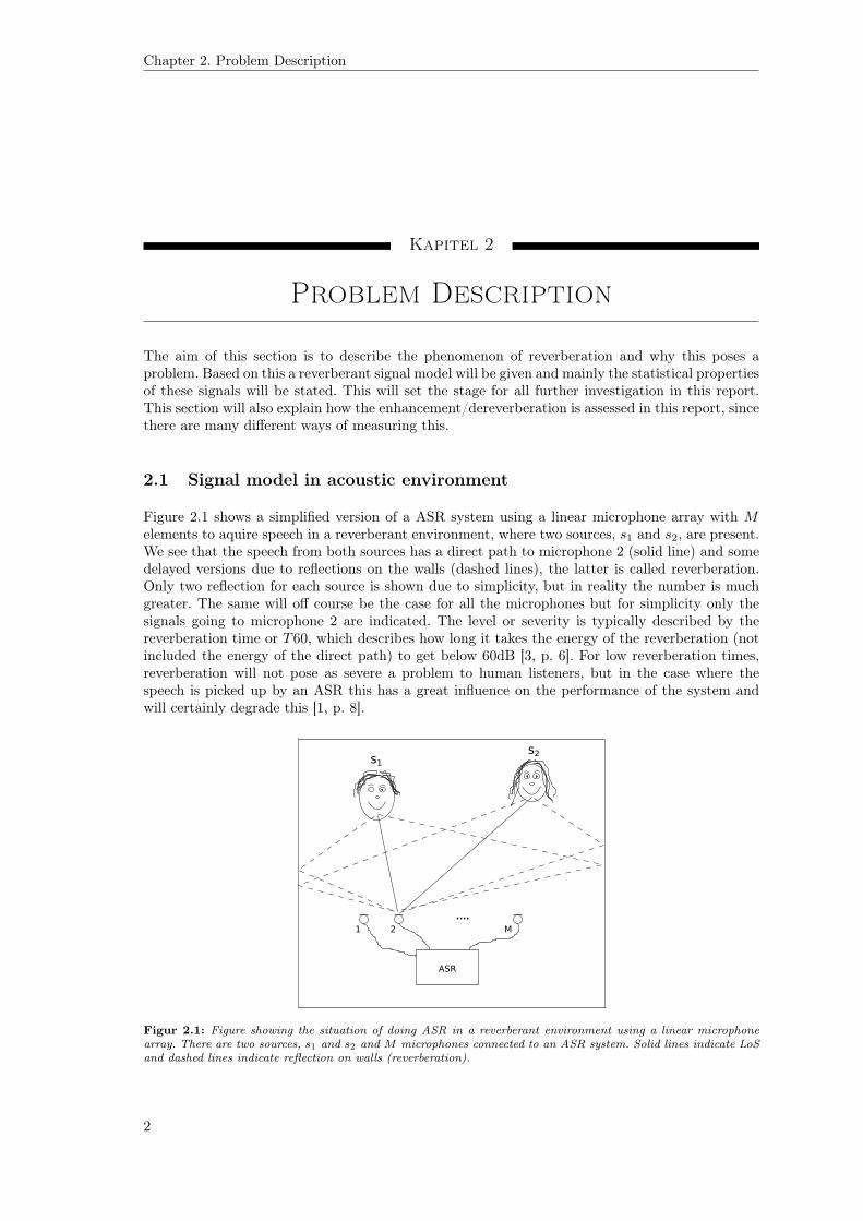
Figure 2.1 shows a simplified version of a ASR system using a linear microphone array with Melements to aquire speech in a reverberant environment, where two sources, s1 and s2, are present.We see that the speech from both sources has a direct path to microphone 2 (solid line) and somedelayed versions due to reflections on the walls (dashed lines), the latter is called reverberation.Only two reflection for each source is shown due to simplicity, but in reality the number is muchgreater. The same will off course be the case for all the microphones but for simplicity only thesignals going to microphone 2 are indicated. The level or severity is typically described by thereverberation time or T60, which describes how long it takes the energy of the reverberation (notincluded the energy of the direct path) to get below 60dB [3, p. 6]. For low reverberation times,reverberation will not pose as severe a problem to human listeners, but in the case where thespeech is picked up by an ASR this has a great influence on the performance of the system andwill certainly degrade this [1, p. 8].
ASR
....
1 2 M
s1s2
Figur 2.1: Figure showing the situation of doing ASR in a reverberant environment using a linear microphonearray. There are two sources, s1 and s2 and M microphones connected to an ASR system. Solid lines indicate LoSand dashed lines indicate reflection on walls (reverberation).
2
Section 2.2. Objective of speech enhancement
We are now able to state a signal model for the signal received at the mth microphone [4, p.68]
ym(n) =
K∑k=1
gm,k(n) ∗ sk(n) + vm(n) (2.1)
where:ym(n) is the output signal from the mth microphone at time index ngm,k(n) is the acoustic impulse response between the kth source and the mth microphone at
time index nsk(n) is the clean signal from the kth source at time index nvm(n) is additive white noise at the mth microphoneK is the number of sources
Normally one is interested in only one of the sources and consider this as the signal of interestand then regard all other sources as interference, but for convenience this is not explicitly statedin the signal model here. To get a better understanding of what is going on in equation 2.1 we willlist the known and assumed properties of the signals.
Source signals, sk(n)
These are the unknown clean speech signals from the sources, and therefore broadband signals.Each speech signal is assumed to be a non-stationary and zero-mean stochastic process. We furtherhave that the source signals are uncorrellated, e.g. E[sk1(n1)sk2(n2)] = 0 for k1, k2 = 1,2,...K,k1 6= k2 and for all n1 and n2.
Acoustic Impulse Response, gm,k(n)
These are unknown and time-variant. Because the reverberation time is between 0.1s and 1s fornormally sized rooms, the length of the Acoustic Impulse Response (AIR)’s is in the order ofthousands [3, p. 8].
Additive noise, vm(n)
We assume that the noise is Additive White Gaussian Noise (AWGN) both temporally and spatially(across microphones), e.g. E[vm(n1)vm(n2)] = 0 for all n1,n2 and n1 6= n2 and E[vm1(n)vm2(n)] =0 for m1,m2 = 1,2,...M , m1 6= m2 and for all n.
Microphone signals, ym(n)
We will assume that all microphone signals are zero-mean. Because every microphone will receivesignals from all sources (with different delays) the microphone signals are correlated with eachother, e.g. E[ym1(n1)ym2(n2)] 6= 0 for all m1,m2 = 1,2,...M and for all n1 and n2.
2.2 Objective of speech enhancement
As mentioned earlier there are mainly two reasons to do speech enhancement, where the first is thecase when a human listener is perceiving the signal, and the second case is when enhancement isneeded in order for an ASR to achieve satisfying performance in terms of Word Error Rate (WER)or PER. This thesis will focus on the last objective.
2.2.1 Suppression vs. Cancellation
Many different methods have been employed trying to eliminate the reverberation of speech andthereby achieve optimum performance of an ASR. All these methods can roughly be divided intotwo main categories as done in [5]. Here the methods are divided in reverberation cancellation andreverberation suppression. The basic idea of the two categories and the differences is now explained.
3
Chapter 2. Problem Description
CancellationWhen trying to cancel out the reverberation effect one aims at estimating the true AIR’s and thenperform an inverse filtering or deconvolution. This is also refered to as blind deconvolution due tothe fact that the AIR’s are estimated blindly. In theory this will yield a perfect reconstruction ofthe true speech signal [4, p. 152], sk(n), but the method has some drawbacks. In order for thismethod to be useful first of all the AIR’s must be estimated. Since the lengths of these are typicallyin the order of hundreds or thousands these can be very difficult to estimate in practice. Also theAIR’s cannot share any common zeros when looking at these in the z-domain as this will result ina rank-deficient filter matrix, thus making it non-invertible [4, p. 152].
SuppressionThese methods primarily relies on optimum filtering by exploiting the statistical properties of thedesired speech source. One example of a suppression method is fixed/adaptive beamforming, whereknowledge of the direction of the desired signal is used to suppress signals impinging from otherdirection. These types of method are generally more robust then cancellation methods becausenothing needs to be estimated, but as a consequence the potential is not as great [5, p. 74].
In this thesis focus will be on suppression methods using multiple microphones.
4
Chapter 3. Array Signal Processing
Kapitel 3
Array Signal Processing
3.1 Array response and signal model
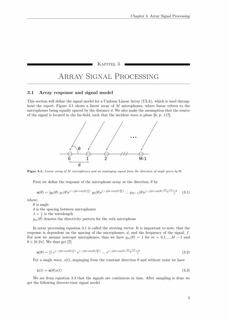
This section will define the signal model for a Uniform Linear Array (ULA), which is used throug-hout the report. Figure 3.1 shows a linear array of M microphones, where linear referes to themicrophones being equally spaced by the distance d. We also make the assumption that the sourceof the signal is located in the far-field, such that the incident wave is plane [6, p. 117].
0 1 2 M-1
...
d
θ
Figur 3.1: Linear array of M microphones and an impinging signal from the direction of angle given by Θ.
First we define the response of the microphone array at the direction, θ by
a(θ) = [g0(θ) g1(θ)e(−j2π cos(θ) dλ ) g2(θ)e(−j2π cos(θ) 2dλ ) ... gM−1(θ)e(−j2π cos(θ)
(M−1)dλ )]T (3.1)
where:θ is angled is the spacing between microphonesλ = c
f is the wavelengthgm(θ) denotes the directivity pattern for the mth microphone
In array processing equation 3.1 is called the steering vector. It is important to note, that theresponse is dependent on the spacing of the microphones, d, and the frequency of the signal, f .For now we assume isotropic microphones, thus we have gm(θ) = 1 for m = 0,1,...,M − 1 andθ ∈ [0; 2π[. We thus get [7]
a(θ) = [1 e(−j2π cos(θ) dλ ) e(−j2π cos(θ) 2dλ ) ... e(−j2π cos(θ)
(M−1)dλ )]T (3.2)
For a single wave, s(t), impinging from the constant direction θ and without noise we have
x(t) = a(θ)s(t) (3.3)
We see from equation 3.3 that the signals are continuous in time. After sampling is done weget the following discrete-time signal model
5
Chapter 3. Array Signal Processing
x(n) = a(θ)s(n) (3.4)
where:n is the sample index
We are now able to define the discrete-time output of the array when K waves are impingingand additive noise is present [7]
x(n) = A(θ)s(n) + v(n) (3.5)
where:A(θ) ∈ CM×K is a matrix, whose columns are the steering vectors corresponding to the impin-
ging signalss(n) ∈ RK×1 is a vector containing the K signals at time nv(n) ∼ N (0,σ2I) is additive noise
A very important observation is that when no noise is present x(n) is contained in the K-dimensional subspace of the M -dimensional signal-subspace, assuming that K < M [7].
3.2 Generalised Sidelobe Canceller (GSC)
This section will explain and derive a classical adaptive beamformer called the Generalised SidelobeCanceller. We start by defining the signal model and scenario. Afterwards the solution is derivedand a practical implementation based on this is explained. At last some simulations are conductedby implementing the beamformer in Matlab.
3.2.1 Problem description
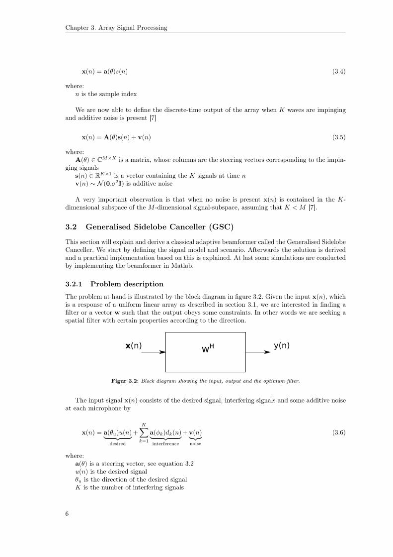
The problem at hand is illustrated by the block diagram in figure 3.2. Given the input x(n), whichis a response of a uniform linear array as described in section 3.1, we are interested in finding afilter or a vector w such that the output obeys some constraints. In other words we are seeking aspatial filter with certain properties according to the direction.
x(n) y(n)wH
Figur 3.2: Block diagram showing the input, output and the optimum filter.
The input signal x(n) consists of the desired signal, interfering signals and some additive noiseat each microphone by
x(n) = a(θu)u(n)︸ ︷︷ ︸desired
+
K∑k=1
a(φk)dk(n)︸ ︷︷ ︸interference
+ v(n)︸︷︷︸noise
(3.6)
where:a(θ) is a steering vector, see equation 3.2u(n) is the desired signalθu is the direction of the desired signalK is the number of interfering signals
6
Section 3.2. Generalised Sidelobe Canceller (GSC)
dk(n) is the kth interfering signalφk is the direction of the kth interfering signal signalv(n) ∼ N (0,σ2I)
3.2.2 Derivation
The GSC is an implementation of a the Linear Constrained Minimum-Variance (LCMV) beam-former [6, p. 120]. Some assumptions are neccessary in order for the GSC to be valid
• The direction of the desired signal is known and does not change over time
• The desired signal is narrowband
The problem of finding the LCMV optimum filter can be stated as an optimization problem,where it is sought to find the filter coefficients w, which yields a minimum output power and atthe same time obey some linear constraints.
min E[|y(n)|2] = E[y(n)y(n)∗] = E[wHx(n)(wHx(n))∗] = wHRxxw
subject to CHw = g (3.7)
where:E is the expectation operatorRxx is the correlation matrix of the input x(n)C is a constraint matrix
The solution to equation 3.7 is found by using the method of Lagrange multipliers and is givenby
wo = R−1xxC(CHR−1xxC)−1g (3.8)
The full derivation of the solution is given in appendix A. There are many ways of constrainingthe problem and thereby choosing C and g [8, p. 514-525]. We see from equation 3.8 that thesolution requires that the covariance matrix of the input signal is known in beforehand. This isnot the case in real-world problems, thus we need to do something else. The next subsection willexplain how using the covariance matrix is avoided.
3.2.3 Implementation
The idea behind the GSC is to divide the M -dimensional signal space into a subspace given bythe constraints and a subspace which is orthogonal to the constraint subspace [8]. We assume theconstraints to be linearly independent and that the number of constraints is lower than the numberof microphones, L < M . The constraint subspace therefor has the dimension L and the dimensionof the orthogonal space is M − L. The range of the constraint subspace is thus given by the spanof the columns of C and we define the matrix B, which column space span the orthogonal space.In the literature the matrix B is called the blocking matrix, so we adopt this. The orthogonalityrequirement can be stated as
CHB = 0 (3.9)
where:0 is a matrix of zeros
7
Chapter 3. Array Signal Processing
We see from 3.9 that the column of B span the null space of CH . The optimum filter is splitinto a contribution from the constraint subspace and a contribution from the orthogonal subspace[8]
wo = wq −wp (3.10)
where:wq is the part from the constraint subspacewp is the part from the orthogonal subspace
wq and wp are found by projecting wo onto C and B, respectively. The projection matrix ontothe constraint space is given by
PC = C(CHC)−1CH (3.11)
We can now find an expression for wq
wq = PCwo (3.12)
= C(CHC)−1CHR−1C(CHR−1C)−1g (3.13)
= C(CHC)−1g (3.14)
An important thing to notice here is that wq does not depend on the statistics of the inputsignal, but only the constraints. Another important thing is in the case where we constrain to haveunit gain in the desired direction, θu, we thus have the following constraint
CHw = a(θu)Hw = 1 (3.15)
This is a special case of the LCMV and is called Minimum-Variance Distortionless Response(MVDR) beamformer [6, p. 119]. We note that the single linear constraint in equation 3.15 is equalto the steering vector in equation 3.2, e.g C = a(θu). By replacing the constraint matrix, C, in thelast expression in equation 3.14 with the single constraint from equation 3.15 and using the factthat C = a(θu), we get
wq = a(θu)(a(θu)Ha(θu)
)−11 =
a(θu)
||a(θu)||22(3.16)
where:||·||2 denotes the euclidian norm.
From comparing equation 3.16 with equation 3.4 we see that wq turns out to be a matchedfilter to the desired signal.
Equation 3.11 can also be used to create a matrix B, which comply with equation 3.9, in thefollowing way
B = I−PC (3.17)
We now take the first M − L columns of B [8, p. 532].It is now possible to find wp in the same way as wq was found. This is however not satisfying
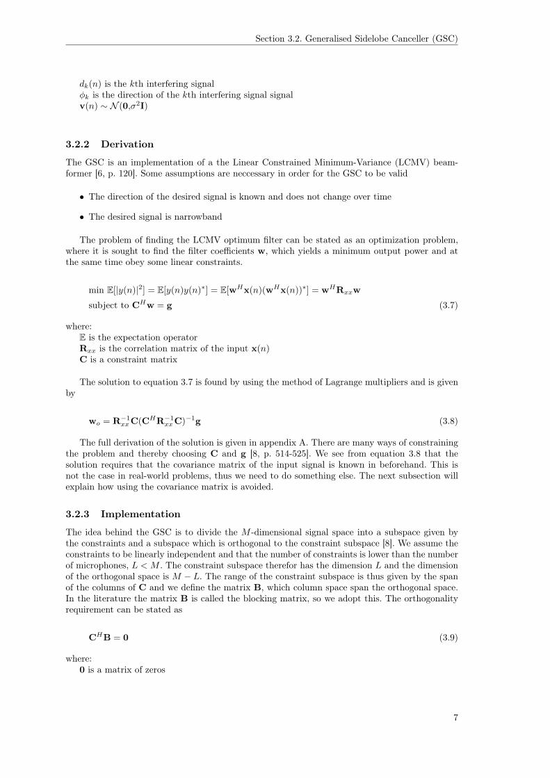
and a better solution exists. We can reformulate the problem into an optimum filtering problem.This is illustrated in figure 3.3.
Figure 3.3 shows how the input signal is split into an upper and lower path. The upper pathmakes sure that unit gain is achieved in the desired direction, and the lower path takes care ofinterference. The lower path is thus implemented as an adaptive filter, since the interference andnoise is not known before hand. In this way the filter can adapt to changing environments. Toensure that the lower path do not conflict with the upper path, the input to the lower path isfirst projected on to the orthogonal space of the constraint space by multiplying with the blockingmatrix, B, hence the name.
8
Section 3.2. Generalised Sidelobe Canceller (GSC)
wq
B wp
∑-
d(n)x(n)
y(n)
e(n)
Z(n)
Figur 3.3: Block diagram of the GSC. The dashed line frames the part, which can be considered as an optimumfilter [6, p. 123].
3.2.4 Simulation
A MATLAB implementation of the GSC has been made, where the adaptive filter in the lowerpath on figure 3.3 is a Normalised Least-Mean-Square (NLMS) adaptive filter [6, p. 320-324]. Theequation for updating the filter weight is given by
w(n+ 1) = w(n) +β
ε+ ||z(n)||22z(n)e∗(n) (3.18)
where:β is the step-size. Should obey 0 < β ≤ 2ε is a small positive constant to ensure numerical stability when ||z(n)||2 is small
It is not the scope of this report to investigate the theory behind adaptive filtering. Threescenarios are chosen to illustrate the effect of the GSC. To keep focus on its ability to suppressinterference and not noise, the simulations were run without adding noise. We construct the sig-nal using a narrowband signal-of-interest and narrowband interference. The signal received bymicrophone m is described by
xm(n) = A cos(2πFn)︸ ︷︷ ︸u(n)
·e−j2πmcos(θ)λu +
K∑k=1
Bk cos(2πfkn+ ψk)︸ ︷︷ ︸sk(n)
·e−j2πmcos(φk)
λk (3.19)
where:A is the amplitude of the desired signalF is the frequency of the desired signalθ is the direction of arrival of the desired signalK is the number of interfering signalsBk is the amplitude of the kth interfering signalfk is the frequency of the kth interfering signalψk is the phase of the kth interfering signalφk is the direction of the kth interfering signal
In both simulation we use the MVDR beamformer given by equation 3.15.
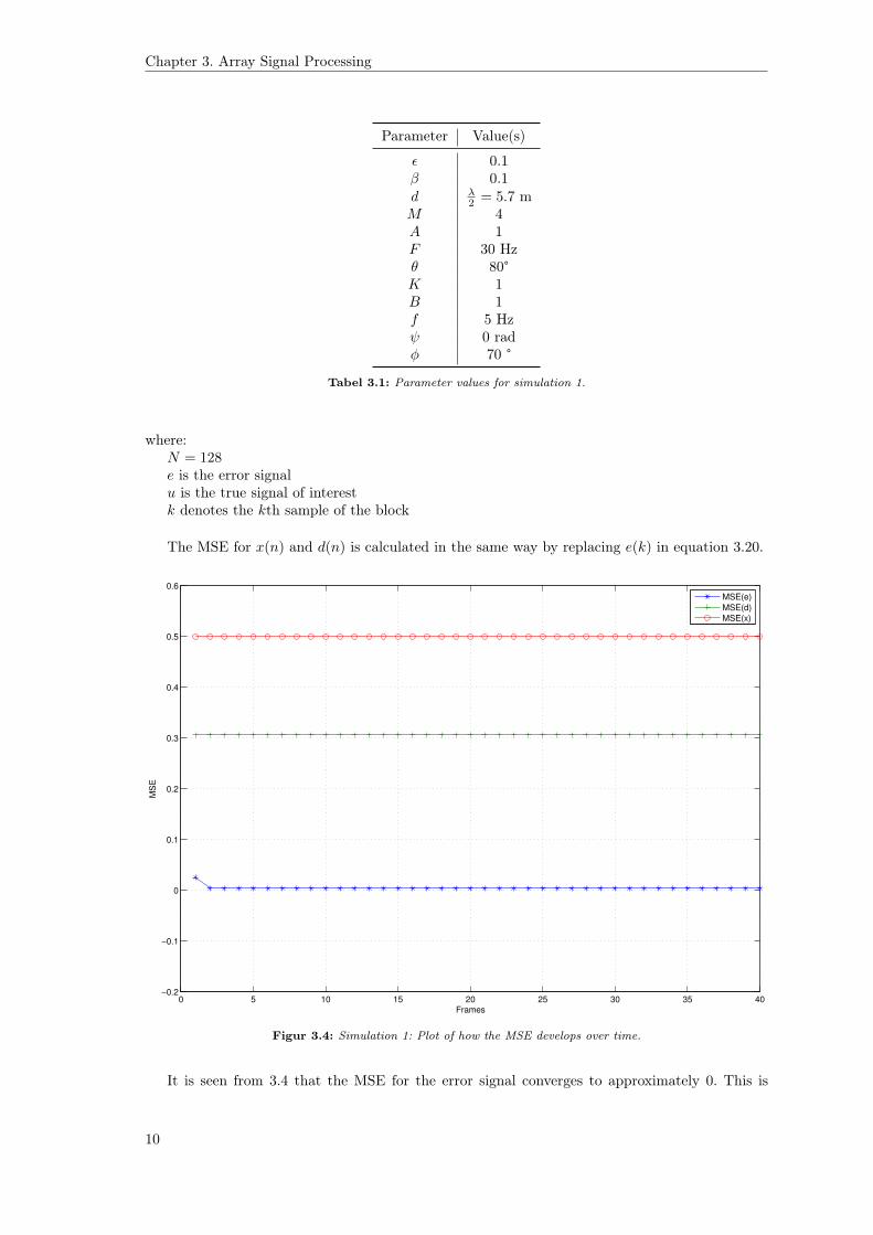
Simulation 1 - Single interfering sourceTable 3.1 shows the settings for this simulation, where only one interfering source is present.
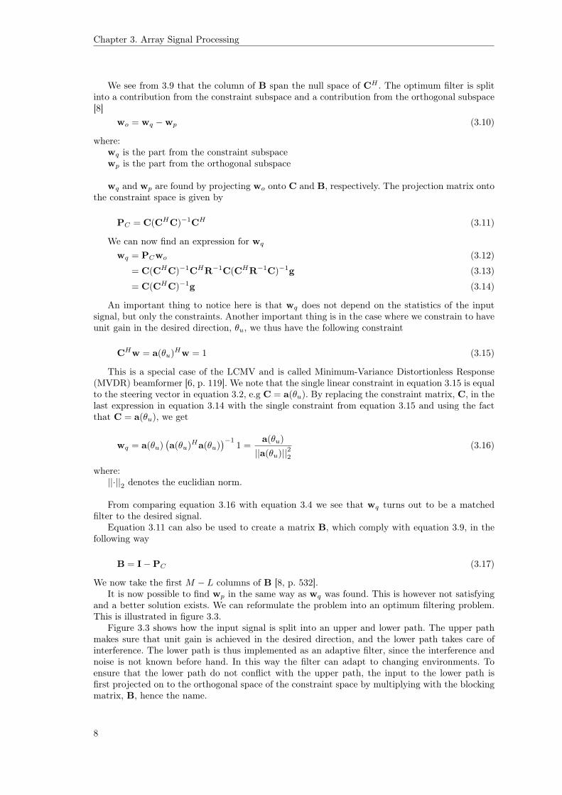
Figure 3.4 shows how the mean-squared error (MSE) develops over time in frames of 128samples for e(n), d(n) and in the case of the raw input from a single microphone x(n). The MSEfor the error signal is estimated by
MSE(e) =1
N
N∑k=1
(u(k)− e(k))2 (3.20)
9
Chapter 3. Array Signal Processing
Parameter Value(s)
ε 0.1β 0.1d λ
2 = 5.7 mM 4A 1F 30 Hzθ 80°K 1B 1f 5 Hzψ 0 radφ 70 °
Tabel 3.1: Parameter values for simulation 1.
where:N = 128e is the error signalu is the true signal of interestk denotes the kth sample of the block
The MSE for x(n) and d(n) is calculated in the same way by replacing e(k) in equation 3.20.
0 5 10 15 20 25 30 35 40−0.2
−0.1
0
0.1
0.2
0.3
0.4
0.5
0.6
Frames
MS
E
MSE(e)
MSE(d)
MSE(x)
Figur 3.4: Simulation 1: Plot of how the MSE develops over time.
It is seen from 3.4 that the MSE for the error signal converges to approximately 0. This is
10
Section 3.2. Generalised Sidelobe Canceller (GSC)
compared to the case when only a single microphone is used and no enhancement is done, wherethe MSE oscillates around approximately 0.5. The last case is when only the matched filter, wq,is used. In this case the MSE is 0.3 and we see that we get an improvement compared to thesingle microphone case, but still not as good as the whole GSC. The GSC clearly outperformsthe matched filter in this case, because the interfering signal has an impinging angle close to thedesired signal together with the fact that the beam of matched filter improves proportionally withthe number of microphones.
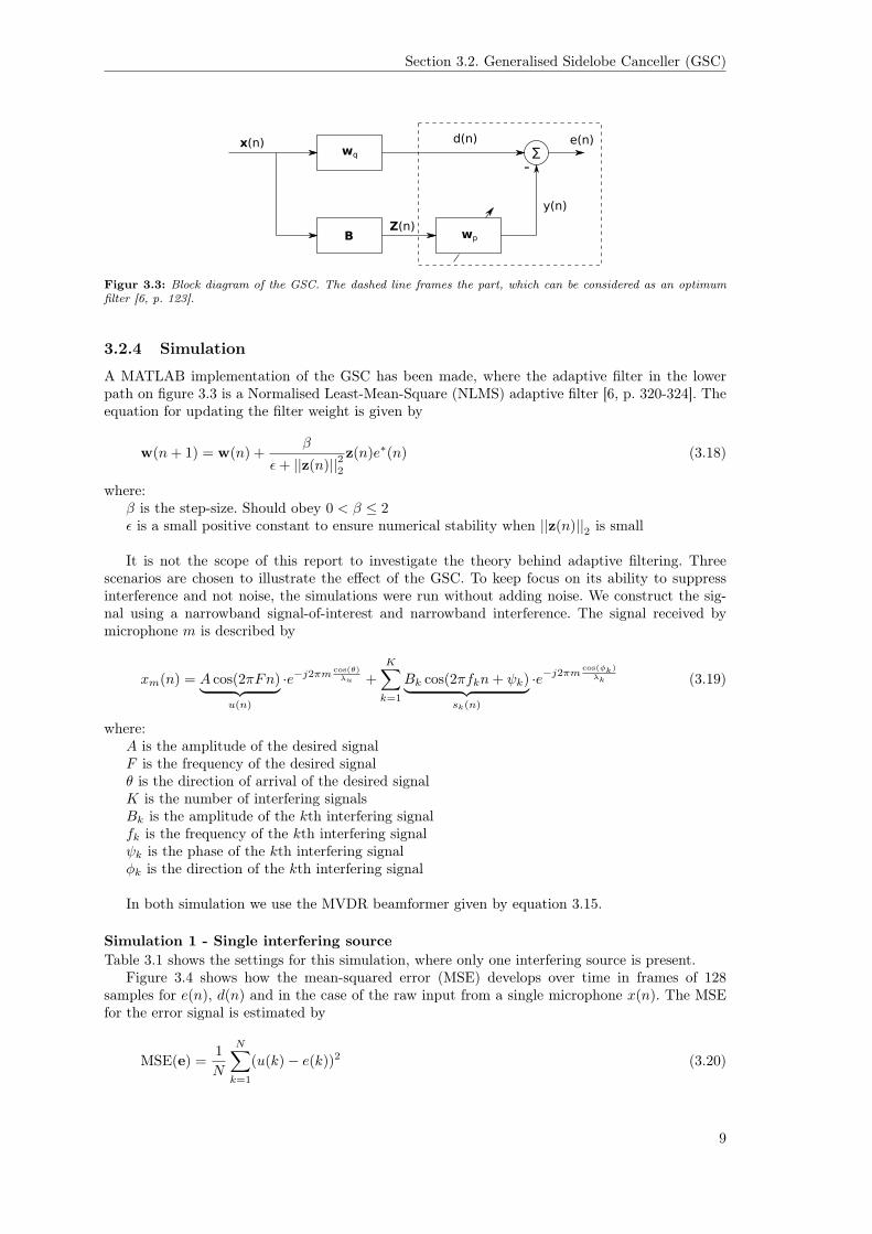
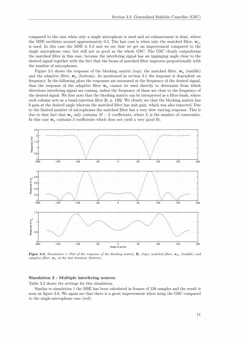
Figure 3.5 shows the response of the blocking matrix (top), the matched filter, wq (middle)and the adaptive filter, wp (bottom). As mentioned in section 3.1 the response is dependent onfrequency. In the following plots the responses are measured at the frequency of the desired signal,thus the response of the adaptive filter wp cannot be used directly to determine from whichdirections interfering signal are coming, unless the frequency of these are close to the frequency ofthe desired signal. We first note that the blocking matrix can be interpreted as a filter-bank, whereeach column acts as a band-rejection filter [6, p. 126]. We clearly see that the blocking matrix has0 gain at the desired angle whereas the matched filter has unit gain, which was also expected. Dueto the limited number of microphones the matched filter has a very slow varying response. This isdue to that fact that wq only contains M − L coefficients, where L is the number of constraints.In this case wq contains 3 coefficients which does not yield a very good fit.
−200 −150 −100 −50 0 50 100 150 2000
0.5
1
1.5
2
2.5
Response o
f B
−200 −150 −100 −50 0 50 100 150 2000
0.2
0.4
0.6
0.8
1
Response o
f w
q
−200 −150 −100 −50 0 50 100 150 2000
0.5
1
1.5
Response o
f w
a
Angle of arrival
Figur 3.5: Simulation 1: Plot of the response of the blocking matrix, B, (top), matched filter, wq, (middle) andadaptive filter, wp at the last iteration (bottom).
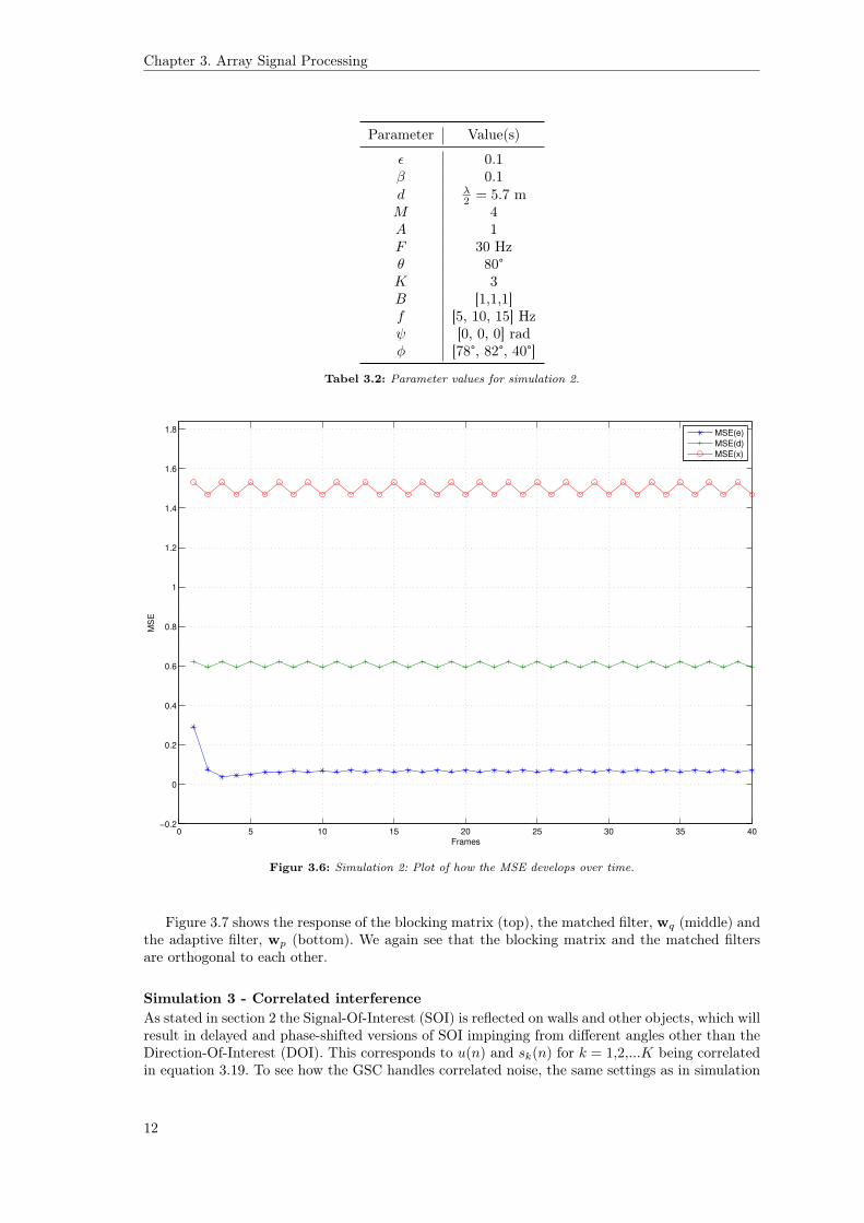
Simulation 2 - Multiple interfering sourcesTable 3.2 shows the settings for this simulation.
Similar to simulation 1 the MSE has been calculated in frames of 128 samples and the result isseen on figure 3.6. We again see that there is a great improvement when using the GSC comparedto the single-microphone case (red).
11
Chapter 3. Array Signal Processing
Parameter Value(s)
ε 0.1β 0.1d λ
2 = 5.7 mM 4A 1F 30 Hzθ 80°K 3B [1,1,1]f [5, 10, 15] Hzψ [0, 0, 0] radφ [78°, 82°, 40°]
Tabel 3.2: Parameter values for simulation 2.
0 5 10 15 20 25 30 35 40−0.2
0
0.2
0.4
0.6
0.8
1
1.2
1.4
1.6
1.8
Frames
MS
E
MSE(e)
MSE(d)
MSE(x)
Figur 3.6: Simulation 2: Plot of how the MSE develops over time.
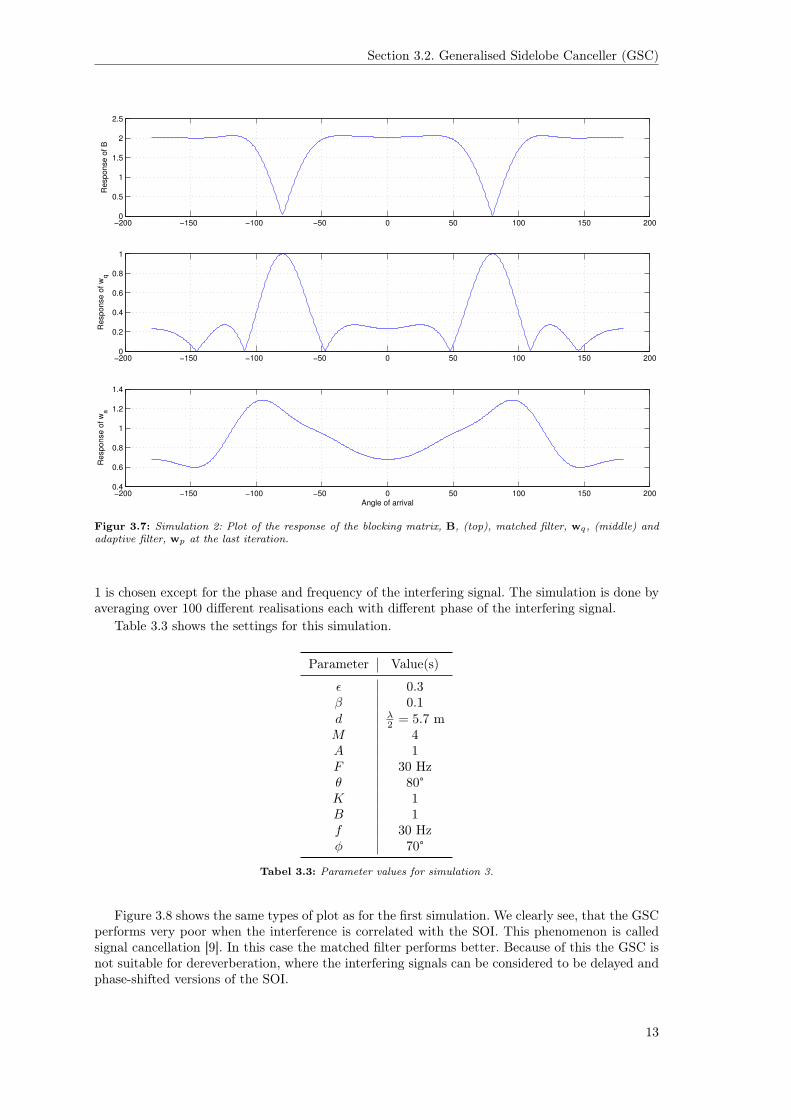
Figure 3.7 shows the response of the blocking matrix (top), the matched filter, wq (middle) andthe adaptive filter, wp (bottom). We again see that the blocking matrix and the matched filtersare orthogonal to each other.
Simulation 3 - Correlated interferenceAs stated in section 2 the Signal-Of-Interest (SOI) is reflected on walls and other objects, which willresult in delayed and phase-shifted versions of SOI impinging from different angles other than theDirection-Of-Interest (DOI). This corresponds to u(n) and sk(n) for k = 1,2,...K being correlatedin equation 3.19. To see how the GSC handles correlated noise, the same settings as in simulation
12
Section 3.2. Generalised Sidelobe Canceller (GSC)
−200 −150 −100 −50 0 50 100 150 2000
0.5
1
1.5
2
2.5
Response o
f B
−200 −150 −100 −50 0 50 100 150 2000
0.2
0.4
0.6
0.8
1
Response o
f w
q
−200 −150 −100 −50 0 50 100 150 2000.4
0.6
0.8
1
1.2
1.4
Response o
f w
a
Angle of arrival
Figur 3.7: Simulation 2: Plot of the response of the blocking matrix, B, (top), matched filter, wq, (middle) andadaptive filter, wp at the last iteration.
1 is chosen except for the phase and frequency of the interfering signal. The simulation is done byaveraging over 100 different realisations each with different phase of the interfering signal.
Table 3.3 shows the settings for this simulation.
Parameter Value(s)
ε 0.3β 0.1d λ
2 = 5.7 mM 4A 1F 30 Hzθ 80°K 1B 1f 30 Hzφ 70°
Tabel 3.3: Parameter values for simulation 3.
Figure 3.8 shows the same types of plot as for the first simulation. We clearly see, that the GSCperforms very poor when the interference is correlated with the SOI. This phenomenon is calledsignal cancellation [9]. In this case the matched filter performs better. Because of this the GSC isnot suitable for dereverberation, where the interfering signals can be considered to be delayed andphase-shifted versions of the SOI.
13
Chapter 3. Array Signal Processing
0 5 10 15 20 25 30 35 40
0.2
0.25
0.3
0.35
0.4
0.45
0.5
0.55
Frames
MS
E
MSE(e)
MSE(d)
MSE(x)
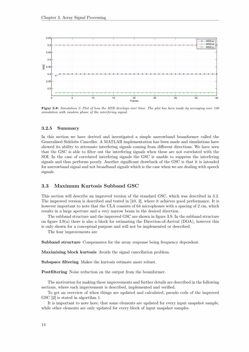
Figur 3.8: Simulation 3: Plot of how the MSE develops over time. The plot has been made by averaging over 100simulation with random phase of the interfering signal.
3.2.5 Summary
In this section we have derived and investigated a simple narrowband beamformer called theGeneralised Sidelobe Canceller. A MATLAB implementation has been made and simulations haveshowed its ability to attenuate interfering signals coming from different directions. We have seenthat the GSC is able to filter out the interfering signals when these are not correlated with theSOI. In the case of correlated interfering signals the GSC is unable to suppress the interferingsignals and thus performs poorly. Another significant drawback of the GSC is that it is intendedfor narrowband signal and not broadband signals which is the case when we are dealing with speechsignals.
3.3 Maximum Kurtosis Subband GSC
This section will describe an improved version of the standard GSC, which was described in 3.2.The improved version is described and tested in [10, 2], where it achieves good performance. It ishowever important to note that the ULA consists of 64 microphones with a spacing of 2 cm, whichresults in a large aperture and a very narrow beam in the desired direction.
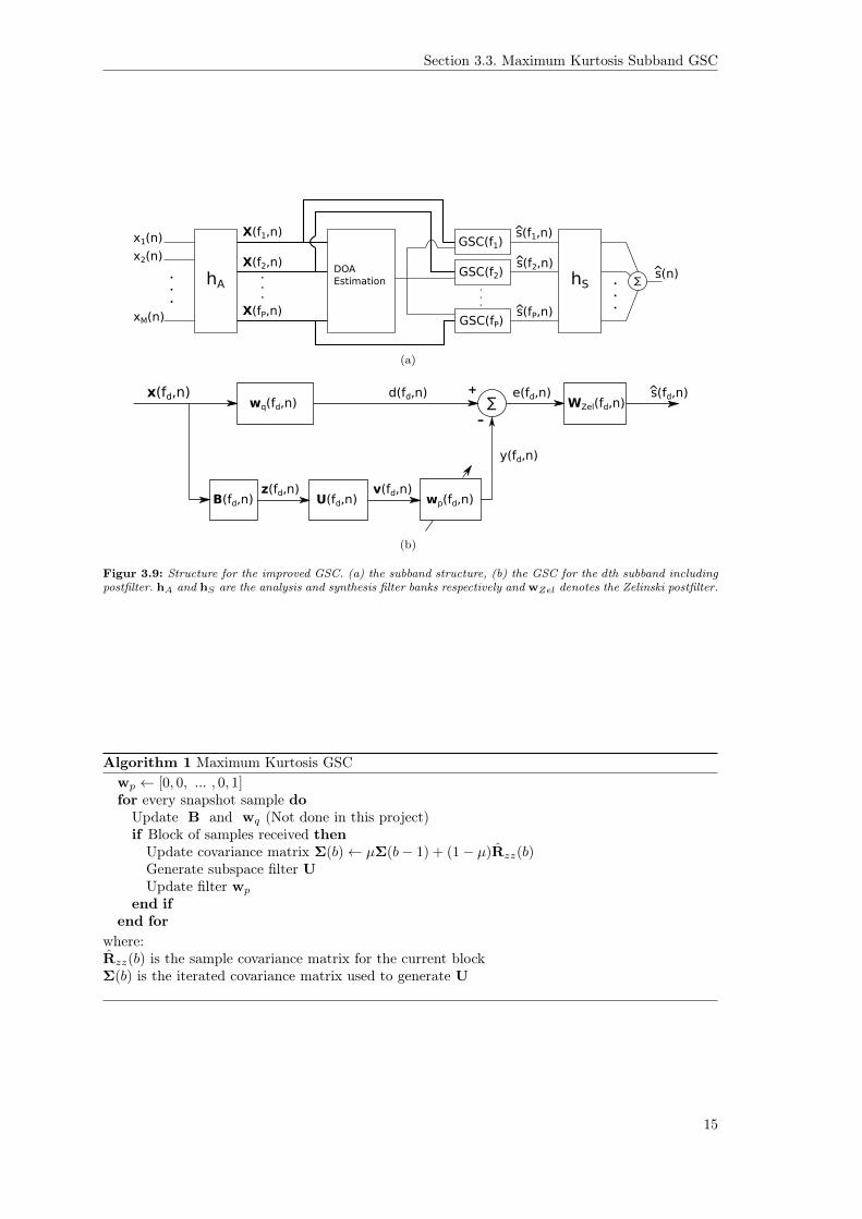
The subband structure and the improved GSC are shown in figure 3.9. In the subband structureon figure 3.9(a) there is also a block for estimating the Direction-of-Arrival (DOA), however thisis only shown for a conceptual purpose and will not be implemented or described.
The four improvements are
Subband structure Compensates for the array response being frequency dependent.
Maximising block kurtosis Avoids the signal cancellation problem.
Subspace filtering Makes the kurtosis estimate more robust.
Postfiltering Noise reduction on the output from the beamformer.
The motivation for making these improvements and further details are described in the followingsections, where each improvement is described, implemented and verified.
To get an overview of when things are updated and calculated, pseudo code of the improvedGSC [2] is stated in algortihm 1.
It is important to note here, that some elements are updated for every input snapshot sample,while other elements are only updated for every block of input snapshot samples.
14
Section 3.3. Maximum Kurtosis Subband GSC
x1(n)
x2(n)
xM(n)
.
.
.
hA
X(f1,n)
X(f2,n)...
X(fP,n)
DOAEstimation
GSC(f1)
GSC(f2)
GSC(fP)
.
.
.
hS ∑...
s(f1,n)^
s(f2,n)^
s(fP,n)^
s(n)^
(a)
wq(fd,n)
B(fd,n) wp(fd,n)
∑-
d(fd,n)x(fd,n)
y(fd,n)
e(fd,n)
z(fd,n)U(fd,n)
+
v(fd,n)
WZel(fd,n)s(fd,n)^
(b)
Figur 3.9: Structure for the improved GSC. (a) the subband structure, (b) the GSC for the dth subband includingpostfilter. hA and hS are the analysis and synthesis filter banks respectively and wZel denotes the Zelinski postfilter.
Algorithm 1 Maximum Kurtosis GSCwp ← [0, 0, ... , 0, 1]for every snapshot sample doUpdate B and wq (Not done in this project)if Block of samples received thenUpdate covariance matrix Σ(b)← µΣ(b− 1) + (1− µ)Rzz(b)Generate subspace filter UUpdate filter wp
end ifend for
where:Rzz(b) is the sample covariance matrix for the current blockΣ(b) is the iterated covariance matrix used to generate U
15
Chapter 3. Array Signal Processing
3.3.1 Filterbank
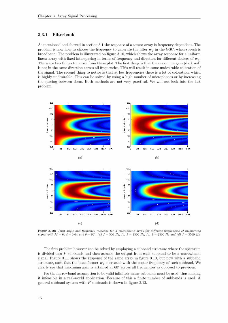
As mentioned and showed in section 3.1 the response of a sensor array is frequency dependent. Theproblem is now how to choose the frequency to generate the filter wq in the GSC, when speech isbroadband. The problem is illustrated on figure 3.10, which shows the array response for a uniformlinear array with fixed interspacing in terms of frequency and direction for different choices of wq.There are two things to notice from these plot. The first thing is that the maximum gain (dark red)is not in the same direction across all frequencies. This will result in some undesirable coloration ofthe signal. The second thing to notice is that at low frequencies there is a lot of coloration, whichis highly undesirable. This can be solved by using a high number of microphones or by increasingthe spacing between them. Both methods are not very practical. We will not look into the lastproblem.
(a) (b)
(c) (d)
Figur 3.10: Joint angle and frequency response for a microphone array for different frequencies of incommingsignal with M = 6, d = 0.04 and θ = 60°. (a) f = 500 Hz, (b) f = 1500 Hz, (c) f = 2500 Hz and (d) f = 3500 Hz.
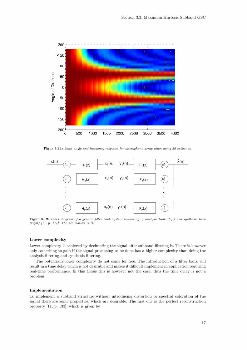
The first problem however can be solved by employing a subband structure where the spectrumis divided into P subbands and then assume the output from each subband to be a narrowbandsignal. Figure 3.11 shows the response of the same array in figure 3.10, but now with a subbandstructure, such that the beamformer wq is created with the center frequency of each subband. Weclearly see that maximum gain is attained at 60° across all frequencies as opposed to previous.
For the narrowband assumption to be valid infinitely many subbands must be used, thus makingit infeasible in a real-world application. Because of this a finite number of subbands is used. Ageneral subband system with P subbands is shown in figure 3.12.
16
Section 3.3. Maximum Kurtosis Subband GSC
Figur 3.11: Joint angle and frequency response for microphone array when using 30 subbands.
H1(z)
H2(z)
HP(z)
F1(z)
F2(z)
FP(z)
x(n) x1(n)
x2(n)
xP(n)
y1(n)
y2(n)
yP(n)
x(n)^D
D
D
D
D
D
.
.
.
.
.
.
Figur 3.12: Block diagram of a general filter bank system consisting of analysis bank (left) and synthesis bank(right) [11, p. 114]. The decimation is D.
Lower complexityLower complexity is achieved by decimating the signal after subband filtering it. There is howeveronly something to gain if the signal processing to be done has a higher complexity than doing theanalysis filtering and synthesis filtering.
The potentially lower complexity do not come for free. The introduction of a filter bank willresult in a time delay which is not desirable and makes it difficult implement in application requiringreal-time performance. In this thesis this is however not the case, thus the time delay is not aproblem.
ImplementationTo implement a subband structure without introducing distortion or spectral coloration of thesignal there are some properties, which are desirable. The first one is the perfect reconstructionproperty [11, p. 133], which is given by
17
Chapter 3. Array Signal Processing
x(n) = c · x(n− n0) (3.21)
where:c is a non-zero constant scalarn0 is some integer
In words equation 3.21 states that in order for perfect reconstruction the output of the filterbank must be a constant scaled and fixed time-delayed version of the input signal. Another designrule is that the decimation factor, D, is chosen to be at maximum equal to the number of subbands,e.g. D ≤ P . In this project it is chosen to use a cosine modulated filter bank, where the analysis-and synthesis filters are given by
hk(n) = 2p0(n) · cos
((k +
1
2
)(n+
N
2
)π
P+ (−1)k
π
4
)(3.22)
fk(n) = 2p0(n) · cos
((k +
1
2
)(n+
N
2
)π
P− (−1)k
π
4
)(3.23)
where:k = 0,1,...,P − 1 is the subband indexn = 0,1,...,N is the sample indexp0(n) is the prototype filter
It has the advantage of being simple to implement. From equation 3.23 we see that the filterbank is realised by finding a low-pass prototype filter and then multiplying by a modulating cosineto get the desired bandpass-filter. It is therefore of importance to chosse the right prototype filter.
VerificationThis section will verify the implementation of a filter bank implementation by applying it to aspeech signal and then comparing to the original signal using spectrograms and MSE. Table 3.4shows the parameter values for the verification.
Parameter Value(s)
P 8D 8N 2048Fs 8kHz
Tabel 3.4: Parameter values for filter bank verification.
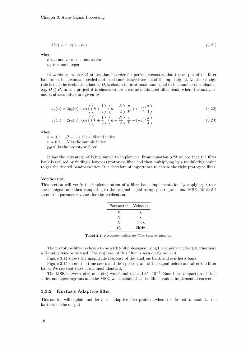
The prototype filter is chosen to be a FIR-filter designed using the window method, furthermorea Hanning window is used. The response of this filter is seen on figure 3.13.
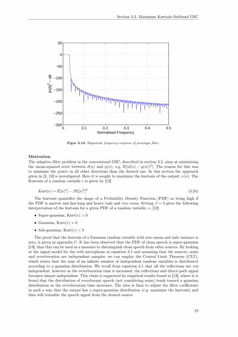
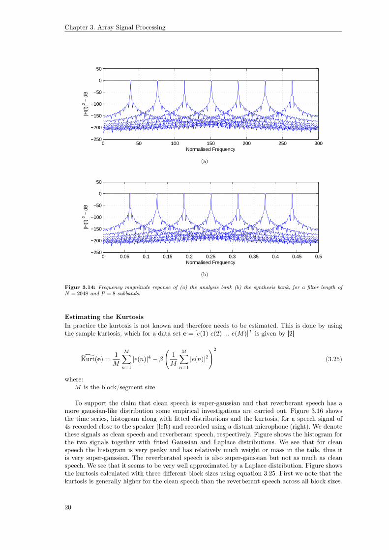
Figure 3.14 shows the magnitude response of the analysis bank and synthesis bank.Figure 3.15 shows the time series and the spectrogram of the signal before and after the filter
bank. We see that these are almost identical.The MSE between x(n) and x(n) was found to be 4.35 · 10−7. Based on comparison of time
series and spectrograms and the MSE, we conclude that the filter bank is implemented correct.
3.3.2 Kurtosis Adaptive filter
This section will explain and derive the adaptive filter problem when it is desired to maximize thekurtosis of the output.
18
Section 3.3. Maximum Kurtosis Subband GSC
0 0.1 0.2 0.3 0.4 0.5−300
−250
−200
−150
−100
−50
0
50
Normalised Frequency
|H(f
)|2 −
dB
Figur 3.13: Magnitude frequency response of prototype filter.
MotivationThe adaptive filter problem in the conventional GSC, described in section 3.2, aims at minimizingthe mean-squared error between d(n) and y(n), e.g. E[(d(n) − y(n))2]. The reason for this wasto minimise the power in all other directions than the desired one. In this section the approachgiven in [2, 10] is investigated. Here it is sought to maximize the kurtosis of the output, e(n). TheKurtosis of a random variable e is given by [12]
Kurt(e) = E[|e|4]− βE[|e|2]2 (3.24)
The kurtosis quantifies the shape of a Probability Density Function (PDF) as being high ifthe PDF is narrow and has long and heavy tails and vice versa. Setting β = 3 gives the followinginterpretation of the kurtosis for a given PDF of a random variable, e, [12]
• Super-gaussian, Kurt(e) > 0
• Gaussian, Kurt(e) = 0
• Sub-gaussian, Kurt(e) < 0
The proof that the kurtosis of a Gaussian random variable with zero mean and unit variance iszero, is given in appendix C. It has been observed that the PDF of clean speech is super-gaussian[13], thus this can be used as a measure to distuinguish clean speech from other sources. By lookingat the signal model for the mth microphone in equation 2.1 and assuming that the sources, noiseand reverberation are independent samples, we can employ the Central Limit Theorem (CLT),which states that the sum of an infinite number of independent random variables is distributedaccording to a gaussian distribution. We recall from equation 2.1 that all the reflections are notindependent, however as the reverberation time is increased, the reflections and direct-path signalbecomes almost independent. This claim is supported by empirical results found in [13], where it isfound that the distribution of reverberant speech (not considering noise) tends toward a gaussiandistribution as the reverberation time increases. The idea is then to adjust the filter coefficientsin such a way that the output has a super-gaussian distribution (e.g. maximize the kurtosis) andthus will resemble the speech signal from the desired source.
19
Chapter 3. Array Signal Processing
0 50 100 150 200 250 300−250
−200
−150
−100
−50
0
50
Normalised Frequency
|H(f
)|2 −
dB
(a)
0 0.05 0.1 0.15 0.2 0.25 0.3 0.35 0.4 0.45 0.5−250
−200
−150
−100
−50
0
50
Normalised Frequency
|H(f
)|2 −
dB
(b)
Figur 3.14: Frequency magnitude reponse of (a) the analysis bank (b) the synthesis bank, for a filter length ofN = 2048 and P = 8 subbands.
Estimating the KurtosisIn practice the kurtosis is not known and therefore needs to be estimated. This is done by usingthe sample kurtosis, which for a data set e = [e(1) e(2) ... e(M)]T is given by [2]
Kurt(e) =1
M
M∑n=1
|e(n)|4 − β
(1
M
M∑n=1
|e(n)|2)2
(3.25)
where:M is the block/segment size
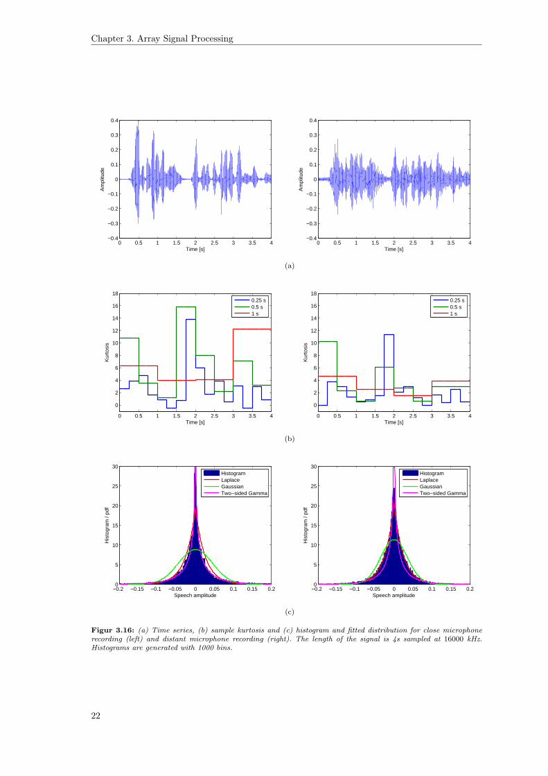
To support the claim that clean speech is super-gaussian and that reverberant speech has amore gaussian-like distribution some empirical investigations are carried out. Figure 3.16 showsthe time series, histogram along with fitted distributions and the kurtosis, for a speech signal of4s recorded close to the speaker (left) and recorded using a distant microphone (right). We denotethese signals as clean speech and reverberant speech, respectively. Figure shows the histogram forthe two signals together with fitted Gaussian and Laplace distributions. We see that for cleanspeech the histogram is very peaky and has relatively much weight or mass in the tails, thus itis very super-gaussian. The reverberated speech is also super-gaussian but not as much as cleanspeech. We see that it seems to be very well approximated by a Laplace distribution. Figure showsthe kurtosis calculated with three different block sizes using equation 3.25. First we note that thekurtosis is generally higher for the clean speech than the reverberant speech across all block sizes.
20
Section 3.3. Maximum Kurtosis Subband GSC
(a)
(b)
Figur 3.15: Spectrogram of (a) x(n) (b) x(n), for a filter length of N = 2048 and P = 8 subbands.
Second it is interesting to see how much the kurtosis varies depending on the block size. Thisindicates, that the block size can have a great influence on the estimation of the kurtosis.
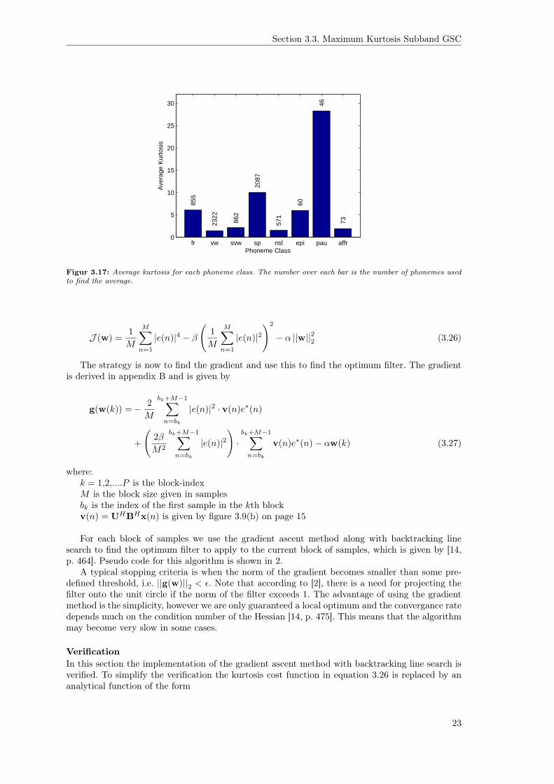
Last, we note that for the clean speech and block size of 0.25s the kurtosis is low for partswhere speech is present, which may indicate that some parts of speech do not have a super-gaussian distribution. To investigate this further the a subset of the TIMIT database was used tofind the average kurtosis of each phoneme group and each phoneme. The average kurtosis of thephoneme classes is seen in figure 3.17. It is interesting to see how much the kurtosis varies acrossphoneme classes and that some classes actually have a very low kurtosis. This shows that someparts of speech do not have a super-gaussian distribution.
The sample kurtosis calculated for the entire time series is 8.8 and 3.6 for clean speech andreverberant speech, respectively. Based on these plots, we thus confirm that reverberant speech isless super-gaussian than clean speech.
There are however drawbacks of using the kurtosis as a measure of non-gaussianity, becausethis is sensitive to outliers, which is not ideal [12, p. 182] and can lead to false estimates of thefilter weights. This issue will be addressed later.
Updating the filter coefficientsAs mentioned in the introduction to the improved GSC the adaptive filter is only updated for everyblock of samples and we are interested in finding the filter which maximizes the sample kurtosisfor the current block of samples. We can define the cost function as the sample kurtosis and add aterm which penalizes large filter coefficents. If this term is not added, it is easily seen that equation3.25 is maximized by making the coefficients of w infinitely big.
21
Chapter 3. Array Signal Processing
0 0.5 1 1.5 2 2.5 3 3.5 4−0.4
−0.3
−0.2
−0.1
0
0.1
0.2
0.3
0.4
Time [s]
Am
plitu
de
0 0.5 1 1.5 2 2.5 3 3.5 4−0.4
−0.3
−0.2
−0.1
0
0.1
0.2
0.3
0.4
Time [s]
Am
plitu
de
(a)
0 0.5 1 1.5 2 2.5 3 3.5 4
0
2
4
6
8
10
12
14
16
18
Time [s]
Kur
tosi
s
0.25 s0.5 s1 s
0 0.5 1 1.5 2 2.5 3 3.5 4
0
2
4
6
8
10
12
14
16
18
Time [s]
Kur
tosi
s
0.25 s0.5 s1 s
(b)
−0.2 −0.15 −0.1 −0.05 0 0.05 0.1 0.15 0.20
5
10
15
20
25
30
Speech amplitude
His
togr
am /
HistogramLaplaceGaussianTwo−sided Gamma
−0.2 −0.15 −0.1 −0.05 0 0.05 0.1 0.15 0.20
5
10
15
20
25
30
Speech amplitude
His
togr
am /
HistogramLaplaceGaussianTwo−sided Gamma
(c)
Figur 3.16: (a) Time series, (b) sample kurtosis and (c) histogram and fitted distribution for close microphonerecording (left) and distant microphone recording (right). The length of the signal is 4s sampled at 16000 kHz.Histograms are generated with 1000 bins.
22
Section 3.3. Maximum Kurtosis Subband GSC
fr vw svw sp nsl epi pau affr0
5
10
15
20
25
30
Phoneme Class
Ave
rage
Kur
tosi
s
855
2322
862
2087
571
60
46
73
Figur 3.17: Average kurtosis for each phoneme class. The number over each bar is the number of phonemes usedto find the average.
J (w) =1
M
M∑n=1
|e(n)|4 − β
(1
M
M∑n=1
|e(n)|2)2
− α ||w||22 (3.26)
The strategy is now to find the gradient and use this to find the optimum filter. The gradientis derived in appendix B and is given by
g(w(k)) =− 2
M
bk+M−1∑n=bk
|e(n)|2 · v(n)e∗(n)
+
(2β
M2
bk+M−1∑n=bk
|e(n)|2)·bk+M−1∑n=bk
v(n)e∗(n)− αw(k) (3.27)
where:k = 1,2,....P is the block-indexM is the block size given in samplesbk is the index of the first sample in the kth blockv(n) = UHBHx(n) is given by figure 3.9(b) on page 15
For each block of samples we use the gradient ascent method along with backtracking linesearch to find the optimum filter to apply to the current block of samples, which is given by [14,p. 464]. Pseudo code for this algorithm is shown in 2.
A typical stopping criteria is when the norm of the gradient becomes smaller than some pre-defined threshold, i.e. ||g(w)||2 < ε. Note that according to [2], there is a need for projecting thefilter onto the unit circle if the norm of the filter exceeds 1. The advantage of using the gradientmethod is the simplicity, however we are only guaranteed a local optimum and the convergance ratedepends much on the condition number of the Hessian [14, p. 475]. This means that the algorithmmay become very slow in some cases.
VerificationIn this section the implementation of the gradient ascent method with backtracking line search isverified. To simplify the verification the kurtosis cost function in equation 3.26 is replaced by ananalytical function of the form
23
Chapter 3. Array Signal Processing
Algorithm 2 Gradient ascent with backtracking line searcht = 1, α ∈]0,0.5], β ∈]0,1] and starting point wwhile Stopping criteria not satisfied dowhile J (w + tg(w)) < J (w) + αt ||g(w)||22 dot← βt
end whilew← w + tg(w)if ||w||2 > 1 then
w = w||w||2
end ifend while
J (w) = wTRw + µwTw (3.28)
and the gradient is thus given as
g(w) = Rw + µw (3.29)
To simplify even further and to be able to visualize the cost function, we constrain the problemto 2 dimenions, i.e. w ∈ R2×1. Based on the gradient we know that the optimum point is a vectorof zeros, i.e. wopt = [0 0]T . Table 3.5 shows how the paramteres are chosen for the verification.
Parameter Value(s)
t 1α 0.1β 0.4µ 0.3ε 0.0001
R
[−0.5 0
0 −1.5
]Tabel 3.5: Parameter values for gradient verification.
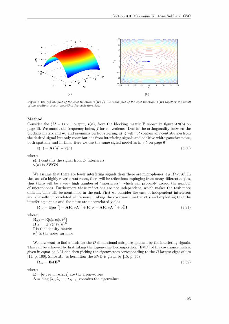
Figure 3.18 shows a 3D plot of the cost function and a contour plot with the results for gradientascent method.
The output of the algorithm after is seen in table 3.6 and we see that it reaches the optimumas expected. We thus conclude that the implementation is correct.
Parameter Value(s)
Number of iterations 49w [−4 · 10−4 −4.5 · 10−33]TJ (w) −3.2 · 10−8
Tabel 3.6: Result for gradient verification.
3.3.3 Subspace filtering
As mentioned in section 3.3.2 the sample kurtosis is sensitive to outliers, thus outliers can causeincorrect updates of the filter, wq. To avoid this the noise subspace is estimated as an average overall noise-vectors making it more robust and one-dimensional.
24
Section 3.3. Maximum Kurtosis Subband GSC
(a)
w1
w2
−20 −15 −10 −5 0 5 10 15 20−20
−15
−10
−5
0
5
10
15
20
(b)
Figur 3.18: (a) 3D plot of the cost function J (w) (b) Contour plot of the cost function J (w) together the resultof the gradient ascent algorithm for each iteration.
MethodConsider the (M − 1) × 1 output, z(n), from the blocking matrix B shown in figure 3.9(b) onpage 15. We ommit the frequency index, f for convenience. Due to the orthogonality between theblocking matrix and wq and assuming perfect steering, z(n) will not contain any contribution fromthe desired signal but only contributions from interfering signals and additive white gaussian noise,both spatially and in time. Here we use the same signal model as in 3.5 on page 6
z(n) = As(n) + v(n) (3.30)
where:s(n) contains the signal from D interferersv(n) is AWGN
We assume that there are fewer interfering signals than there are microphones, e.g. D < M . Inthe case of a highly reverberant room, there will be reflections impinging from many different angles,thus there will be a very high number of "interferers", which will probably exceed the numberof microphones. Furthermore these reflections are not independent, which makes the task moredifficult. This will be mentioned in the end. First we consider the case of independent interferersand spatially uncorrelated white noise. Taking the covariance matrix of z and exploiting that theinterfering signals and the noise are uncorrelated yields
Rzz = E[zzH ] = ARzSAH + RzV = ARzSAH + σ2V I (3.31)
where:RzS = E[s(n)s(n)H ]RzV = E[v(n)v(n)H ]I is the identity matrixσ2V is the noise-variance
We now want to find a basis for the D-dimensional subspace spanned by the interfering signals.This can be achieved by first taking the Eigenvalue Decomposition (EVD) of the covariance matrixgiven in equation 3.31 and then picking the eigenvectors corresponding to the D largest eigenvalues[15, p. 166]. Since Rzz is hermitian the EVD is given by [15, p. 348]
Rzz = EΛEH (3.32)
where:E = [e1, e2, ..., eM−1] are the eigenvectorsΛ = diag [λ1, λ2, ..., λM−1] contains the eigenvalues
25
Chapter 3. Array Signal Processing
When not taking reflections into consideration, the eigenvalues attain the following values whenthey are sorted in descending order [15, p. 166]
λk =
{σ2S + σ2
V for 1 ≤ k ≤ Dσ2V for D + 1 ≤ k ≤M
Based on this we can now define our signal subspace as SS = R{e1, e2, ..., eD} and our noisesubspace as SV = R{eD+1, eD+2, ..., eM−1}, where R{·} denotes the range operator [15]. Thesubspace filter is now constructed in the following way
U = [e1, e2, ..., eD, eV ] (3.33)
where:eV =
∑M−1−Dk=1 eD+k
We see that we have seperated the signal and noise subspaces and reduced the noise subspaceto be of one dimension instead of M −D − 1 by making an average noise vector. This makes theestimation of the noise much more robust and reduces the dimensionality in the case where manymicrophones are used.
As mentioned earlier, when many reflections are present the number of signals will exceed thenumber of microphones, e.g. D > M , which makes this method useless. However some reflectionsmay have a very small amplitude compared to the noise-variance and can therefore be neglected.Another problem arise if the signals are perfectly correlated, then it is impossible to divide therange of the covariance matrix into a signal- and noise subspace [16, p. 378].
Choosing the size of signal subspace and noise subspaceIt is necessary to find a robust and automatic way of estimating how many eigenvectors the signalsubspace and noise subspace comprises of. In [2] it is suggested to use a measure called contributionratio and then threshold on this. The contribution ratio for the ith eigenvector is given by
Ci =λi∑M−1
k=1 λk(3.34)
We then decide if an eigenvector belongs to either the signal subspace or the noise subspaceby thresholding on Ci, if Ci ≥ threshold then eigenvector ei belongs to the signal subspace and ifnot, then it belongs to the noise subspace.
3.3.4 Postfiltering
So far attention has been given to suppress interfering signals and not reducing the noise in equation3.5. This section describes how to reduce noise after beamforming has been applied, hence the namepostfiltering. We assume that the true signal has been corrupted by AWGN, thus the signal modelfor the output of the GSC can be described in the following way:
e(n) = s(n) + w(n) (3.35)
where:e(n) is the output from the GSC at time-index ns(n) is the true signal at time-index nw(n) is AWGN at time-index n
To reduce the noise, we can apply the well-known Wiener-filter [17, p. 612]. In order for theuse of this filter to be valid, s(n) and w(n) must be Wide Sense Stationary (WSS) processes anduncorrelated, E[s(n1)w(n2)] = 0 for all n1 and n2. We assume that w(n) obey the assumptions, butas mentioned in section 2 the source signals are non-stationary, hence s(n) is also non-stationary,
26
Section 3.3. Maximum Kurtosis Subband GSC
which violates the WSS assumption. This can however be overcome by considering frames of 20−30ms seperately. The Wiener-filter seeks to find a linear filter, h, which minimizes the MSE given by
E[(s(n)− s(n))2] (3.36)
where:s(n) =
∞∑k=−∞
h(k)e(n− k)
The solution is given by
H(f) =Ps(f)
Ps(f) + Pw(f)=Ps(f)
Pe(f)(3.37)
where:H(f) is the frequency-domain Wiener-filterPs(f) and Pw(f) are the Power Spectral Density (PSD) of s(n) and w(n), respectivelyPe(f) is the PSD of e(n) = s(n) + w(n)
The time-domain filter can then be obtained by applying the inverse Fourier Transform onH(f). Since we do not know Ps(f) and Pw(f), these must be estimated in some way, which willbe described next.
Zelinski postfilteringSince the signal, s(n), can only be considered WSS in frames of 20− 30 ms the PSD’s cannot beestimated by averaging over a long time series, in other words we need to estimate the PSD’s usingonly data from the current frame. One possibility is to assume ergodicity to split the data intosmaller sets and then do ensemble averaging. However this results in a degradation of resolutionin the frequency domain, which is not desirable. This problem can be tackled by using Zelinskipostfiltering [18], where the method refers to estimating the PSD’s and not the actual filter. Thismethod uses the fact that multiple microphone signals are present. We assume the following signalmodel (same as in equation 2.1) for the signal at the mth microphone
ym(n) =
K∑k=1
gm,k(n) ∗ sk(n) + vm(n) (3.38)
and also that each microphone signal, m = 1,...,M , has been compensated for delay suchthat they are aligned according to the desired direction. This compensation method will not bedescribed in this report. Using the signal model we can now find Ps(f) and Pe(f).
Estimating Pe(f)
Zelinski postfiltering estimates Pe(f) by estimating the PSD for each of the microphone signalsand then average over them. The PSD of ym(n) is given as [17, p. 569]
E[Y ∗m(f)Ym(f)] = E
[(K∑k=1
Gm,k(f)Sk(f) + Vm(f)
)∗( K∑k=1
Gm,k(f)Sk(f) + Vm(f)
)](3.39)
where:S(f) is the Discrete Fourier Transform of s(n)
For simplicity we assume that K = 2, which yieldsE[Y ∗m(f)Ym(f)] =E[(G∗m,1(f)S∗1 (f) +G∗m,2(f)S∗2 (f) + V ∗m(f))(Gm,1(f)S1(f) (3.40)
+Gm,2(f)S2(f) + Vm(f))]
=E[G∗m,1(f)S∗1 (f)Gm,1(f)S1(f) +G∗m,1(f)S∗1 (f)Gm,2(f)S2(f)+ (3.41)
G∗m,1(f)S∗1 (f)Vm(f) +G∗m,2(f)S∗2 (f)Gm,1(f)S1(f)+
G∗m,2(f)S∗2 (f)Gm,2(f)S2(f) +G∗m,2(f)S∗2 (f)Vm(f)+
V ∗m(f)Gm,1(f)S1(f) + V ∗m(f)Gm,2(f)S2(f) + V ∗m(f)Vm(f)]
27
Chapter 3. Array Signal Processing
All the cross-terms equal zero due to the assumtions that all sources are uncorrelated andzero-mean [17, p. 651] resulting in
E[Y ∗m(f)Ym(f)] = |Gm,1(f)|2 E[|S1(f)|2]︸ ︷︷ ︸Ps1 (f)
+|Gm,2(f)|2 E[|S2(f)|2]︸ ︷︷ ︸Ps2 (f)
+E[|Vm(f)|2]︸ ︷︷ ︸Pvm (f)
(3.42)
We can thus estimate Pe(f) by taking the power of the Discrete Fourier Transform (DFT) ofeach of the microphone signals and then average over them, which can be stated as
Pe(f) =1
M
M∑m=1
|F(ym(n))|2 (3.43)
where:Pe(f) denotes the estimate of Pe(f)M is the number of microphonesF() denotes the Fourier Transform
There are two things to notice from equation 3.42. The first thing is that assuming our sourceof interest is s1(n) and that the beamformer perfectly removes all other (K − 1) sources, thenequation 3.35 can be written as
e(n) = s1(n) + w(n) (3.44)(3.45)
and the PSD of e(n) is given by
Pe(f) = Ps1(f) + Pw(f) (3.46)
Comparing equation 3.42 and equation 3.46 it is seen that Pe(f) is overestimated by the sum ofthe PSD of each of the interfering signals. Another thing that is also seen by comparing equation3.42 and equation 3.46 is that unless Pw(f) = Pvm(f) the noise is also overestimated. It is thusnot taken into consideration that the beamformer itself will remove some of the noise makingPw(f) ≤ Pvm(f) for all f .
Estimating Ps(f)
Pe(f) can be estimated by taking the cross-spectrum of the microphone signals and assuming thatthe noise for two different microphones are uncorrelated, e.g. E[vm(k)vp(k)] for m,p = 1,...,M andm 6= p. The cross-spectrum is given by
E[y∗m(f)yp(f)] = E
[(K∑k=1
Gm,k(f)Sk(f) + Vm(f)
)∗( K∑k=1
Gp,k(f)Sk(f) + Vp(f)
)](3.47)
For simplicity we again assume K = 2, which yields
E[Y ∗m(f)Yp(f)] =E[(G∗m,1(f)S∗1 (f) +G∗m,2(f)S∗2 (f) + V ∗m(f))(Gp,1(f)S1(f)+ (3.48)
Gp,2(f)S2(f) + Vp(f))]
=E[G∗m,1(f)S∗1 (f)Gp,1(f)S1(f) +G∗m,1(f)S∗1 (f)Gp,2(f)S2(f)+ (3.49)
G∗m,1(f)S∗1 (f)Vp(f) +G∗m,2(f)S∗2 (f)Gp,1(f)S1(f)+
G∗m,2(f)S∗2 (f)Gp,2(f)S2(f) +G∗m,2(f)S∗2 (f)Vp(f)+
V ∗m(f)Gp,1(f)S1(f) + V ∗m(f)Gp,2(f)S2(f) + V ∗m(f)Vp(f)]
Again all the cross-terms are equal to zero due to the same assumption as before, and we thusget
E[Y ∗m(f)Yp(f)] = G∗m,1(f)Gp,1(f)E[|S1(f)|2]︸ ︷︷ ︸Ps1 (f)
+G∗m,2(f)Gp,2(f)E[|S2(f)|2]︸ ︷︷ ︸Ps2 (f)
(3.50)
28
Section 3.3. Maximum Kurtosis Subband GSC
Ps(f) can now be estimated by first estimating all possible cross-spectra and then average overthem. This can be stated by
Ps(f) =2
M(M − 1)Re
[M−1∑m=1
M∑q=m+1
F(ym(n))∗F(yq(n))
](3.51)
where:Re[·] denotes the Real-operator
Taking only the real part of the estimate is justified by the fact that the true PSD of s(n) isreal-valued [17, p. 573].
From equation 3.50 we again see that in the case where all interfering sources are removed, thePSD of s(n) = s1(n) is overestimated.
Combining the two estimates of the PSD’s we get the following
H(f) =Ps(f)
Pe(f)=
2M(M−1)Re
[∑M−1m=1
∑Mq=m+1 F(ym(n))∗F(yq(n))
]1M
∑Mm=1 |F(ym(n))|2
(3.52)
VerificationIn this section the implementation of Zelinski postfiltering is verified by running a small numericalexample as in section 3.2.4 on page 9. We use the signal-to-noise plus interference ratio (SNIR) asa measure of quality, which is defined as
SNIRdB = 10 · log10
(PS
PI + PN
)(3.53)
where:PS is the power of the desired signalPI is the power of the interfering signalPN is the power of the noise
When no interference is present SNIR corresponds to the well-known signal-to-noise ratio(SNR). The verification is done by sweeping over a range of input SNIR and then calculate theoutput SNIR in case 1: narrowband where no interference is present, case 2: narrowband whena single interferer is present, and case 3: real speech from TIMIT database. In all cases we usethe same signal model as in equation 3.19 in section 3.2.4 on page 9 and the same settings unlessstated otherwise. Furthermore the postfiltering is implemented using the overlap-add method, thusa specific window and overlap has to be chosen. The settings for both narrowband cases (1 and 2)are given in table 3.7
Case 1 and 2
Parameter Value
Fs 256 HzN 8192
Number of simulation pr. SNIR 5Window HanningOverlap 50%
Postfilter block size 32 samples = 12.5 ms
Tabel 3.7: Parameter values for postfilter.
29
Chapter 3. Array Signal Processing
Parameter Value
d λ2 = 7.6 m
M 5A 1F 45 Hzθ 90°
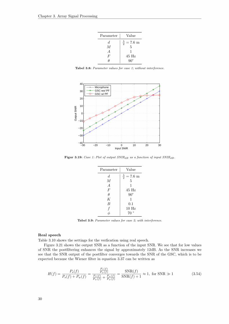
Tabel 3.8: Parameter values for case 1; without interference.
−30 −20 −10 0 10 20 30−40
−30
−20
−10
0
10
20
30
40
Input SNIR
Out
put S
NIR
MicrophoneGSC wo/ PFGSC w/ PF
Figur 3.19: Case 1: Plot of output SNIRdB as a function of input SNIRdB.
Parameter Value
d λ2 = 7.6 m
M 5A 1F 45 Hzθ 90°K 1B 0.1f 10 Hzφ 70 °
Tabel 3.9: Parameter values for case 2; with interference.
Real speechTable 3.10 shows the settings for the verfication using real speech.
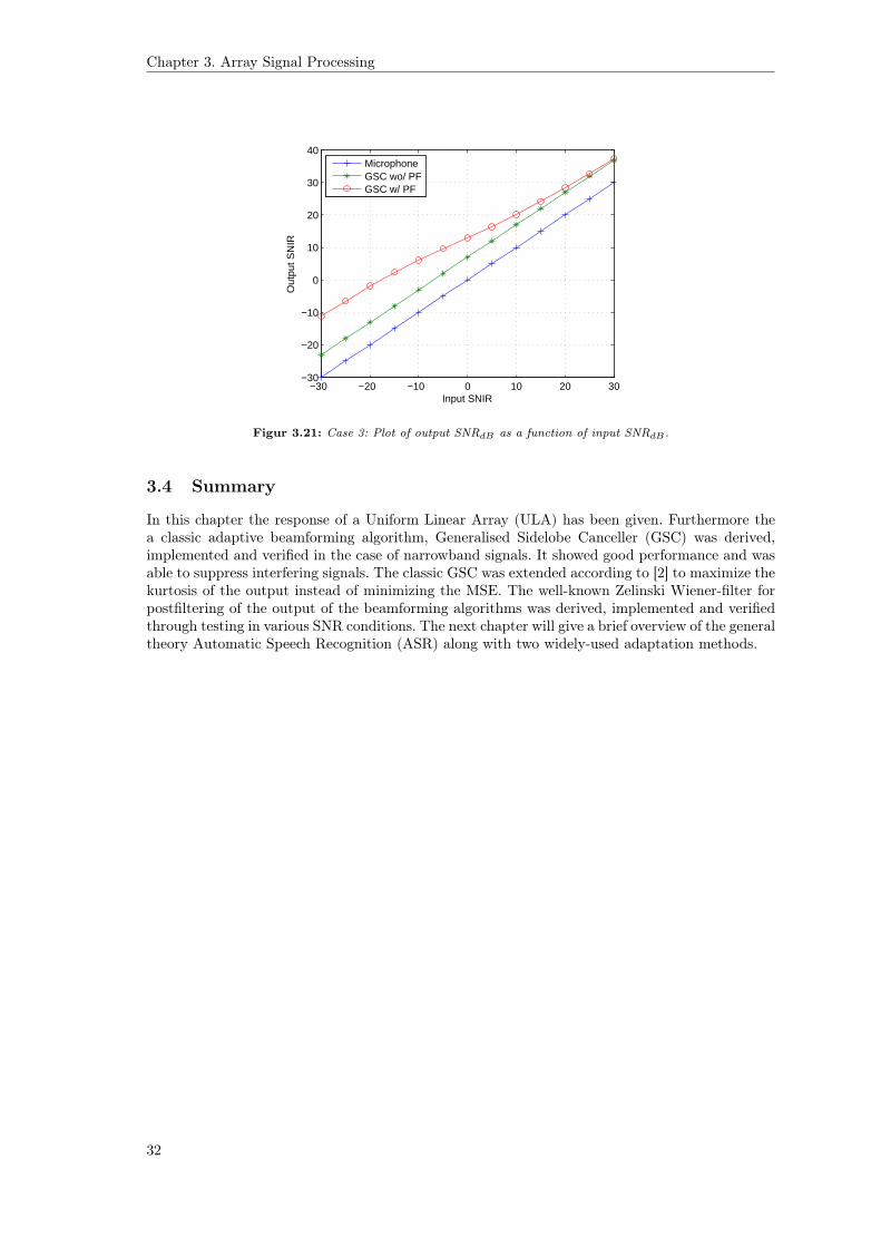
Figure 3.21 shows the output SNR as a function of the input SNR. We see that for low valuesof SNR the postfiltering enhances the signal by approximately 12dB. As the SNR increases wesee that the SNR output of the postfilter converges towards the SNR of the GSC, which is to beexpected because the Wiener filter in equation 3.37 can be written as
H(f) =Ps(f)
Ps(f) + Pw(f)=
Ps(f)Pw(f)
Ps(f)Pw(f) + Pw(f)
Pw(f)
=SNR(f)
SNR(f) + 1≈ 1, for SNR� 1 (3.54)
30
Section 3.3. Maximum Kurtosis Subband GSC
−30 −20 −10 0 10 20−30
−20
−10
0
10
20
30
Input SNIR
Out
put S
NIR
MicrophoneGSC wo/ PFGSC w/ PF
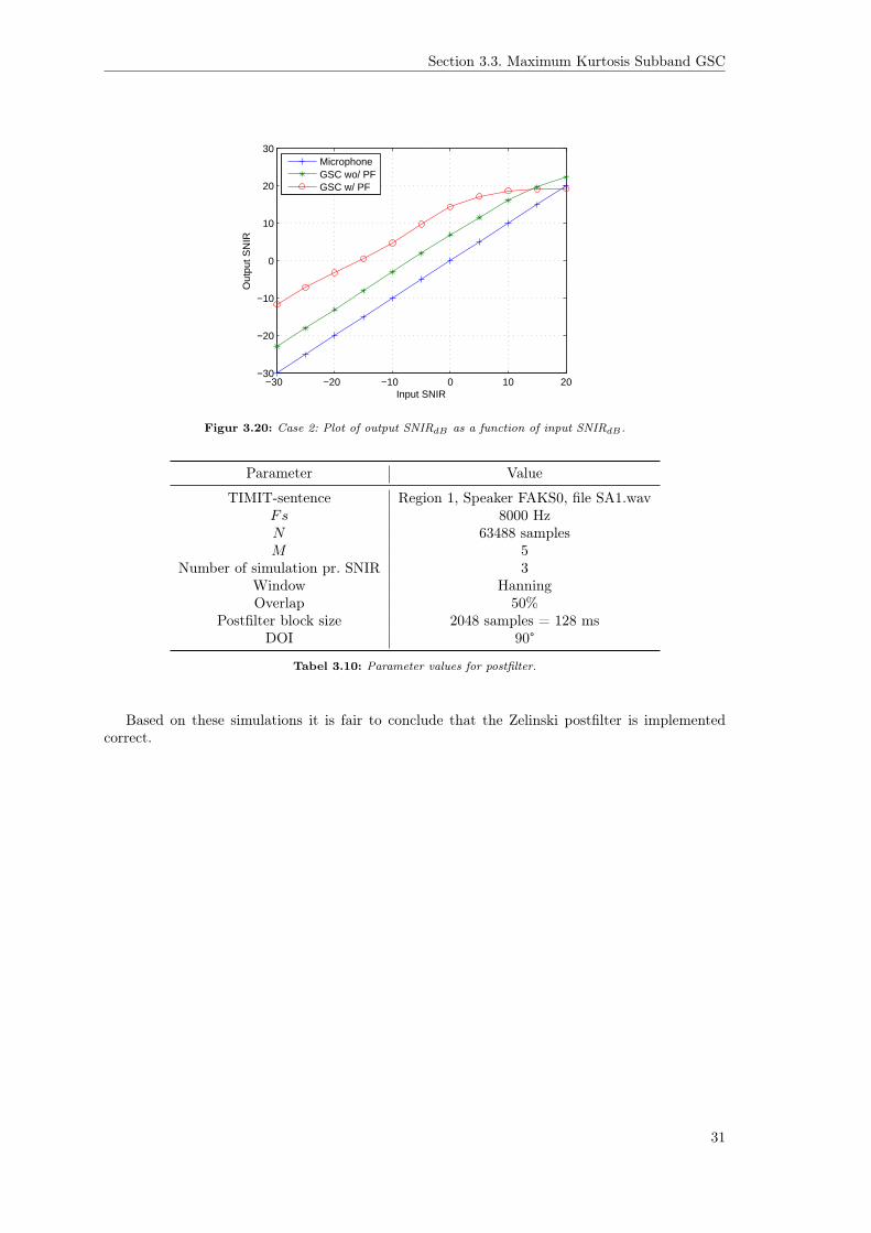
Figur 3.20: Case 2: Plot of output SNIRdB as a function of input SNIRdB.
Parameter Value
TIMIT-sentence Region 1, Speaker FAKS0, file SA1.wavFs 8000 HzN 63488 samplesM 5
Number of simulation pr. SNIR 3Window HanningOverlap 50%
Postfilter block size 2048 samples = 128 msDOI 90°
Tabel 3.10: Parameter values for postfilter.
Based on these simulations it is fair to conclude that the Zelinski postfilter is implementedcorrect.
31
Chapter 3. Array Signal Processing
−30 −20 −10 0 10 20 30−30
−20
−10
0
10
20
30
40
Input SNIR
Out
put S
NIR
MicrophoneGSC wo/ PFGSC w/ PF
Figur 3.21: Case 3: Plot of output SNRdB as a function of input SNRdB.
3.4 Summary
In this chapter the response of a Uniform Linear Array (ULA) has been given. Furthermore thea classic adaptive beamforming algorithm, Generalised Sidelobe Canceller (GSC) was derived,implemented and verified in the case of narrowband signals. It showed good performance and wasable to suppress interfering signals. The classic GSC was extended according to [2] to maximize thekurtosis of the output instead of minimizing the MSE. The well-known Zelinski Wiener-filter forpostfiltering of the output of the beamforming algorithms was derived, implemented and verifiedthrough testing in various SNR conditions. The next chapter will give a brief overview of the generaltheory Automatic Speech Recognition (ASR) along with two widely-used adaptation methods.
32
Chapter 4. Speech Recognition
Kapitel 4
Speech Recognition
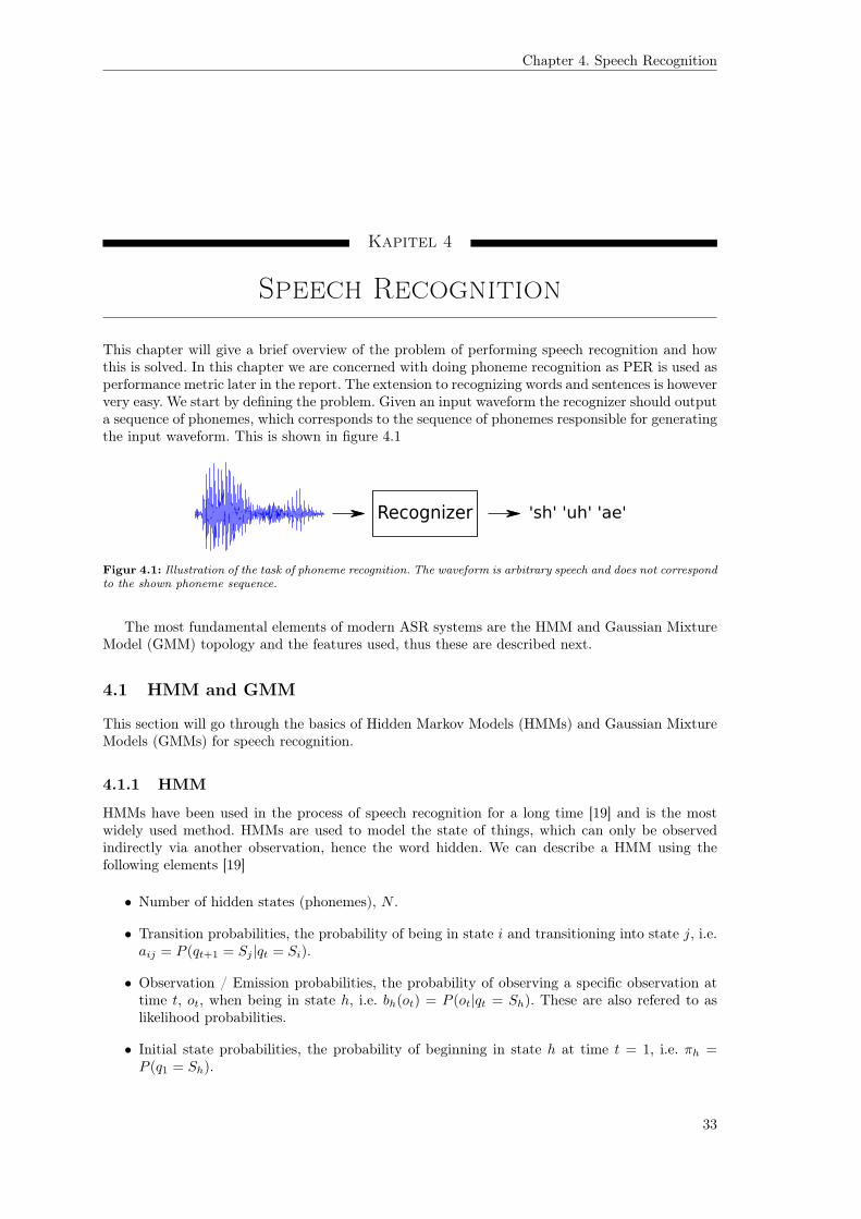
This chapter will give a brief overview of the problem of performing speech recognition and howthis is solved. In this chapter we are concerned with doing phoneme recognition as PER is used asperformance metric later in the report. The extension to recognizing words and sentences is howeververy easy. We start by defining the problem. Given an input waveform the recognizer should outputa sequence of phonemes, which corresponds to the sequence of phonemes responsible for generatingthe input waveform. This is shown in figure 4.1
Recognizer 'sh' 'uh' 'ae'
Figur 4.1: Illustration of the task of phoneme recognition. The waveform is arbitrary speech and does not correspondto the shown phoneme sequence.
The most fundamental elements of modern ASR systems are the HMM and Gaussian MixtureModel (GMM) topology and the features used, thus these are described next.
4.1 HMM and GMM
This section will go through the basics of Hidden Markov Models (HMMs) and Gaussian MixtureModels (GMMs) for speech recognition.
4.1.1 HMM
HMMs have been used in the process of speech recognition for a long time [19] and is the mostwidely used method. HMMs are used to model the state of things, which can only be observedindirectly via another observation, hence the word hidden. We can describe a HMM using thefollowing elements [19]
• Number of hidden states (phonemes), N .
• Transition probabilities, the probability of being in state i and transitioning into state j, i.e.aij = P (qt+1 = Sj |qt = Si).
• Observation / Emission probabilities, the probability of observing a specific observation attime t, ot, when being in state h, i.e. bh(ot) = P (ot|qt = Sh). These are also refered to aslikelihood probabilities.
• Initial state probabilities, the probability of beginning in state h at time t = 1, i.e. πh =P (q1 = Sh).
33
Chapter 4. Speech Recognition
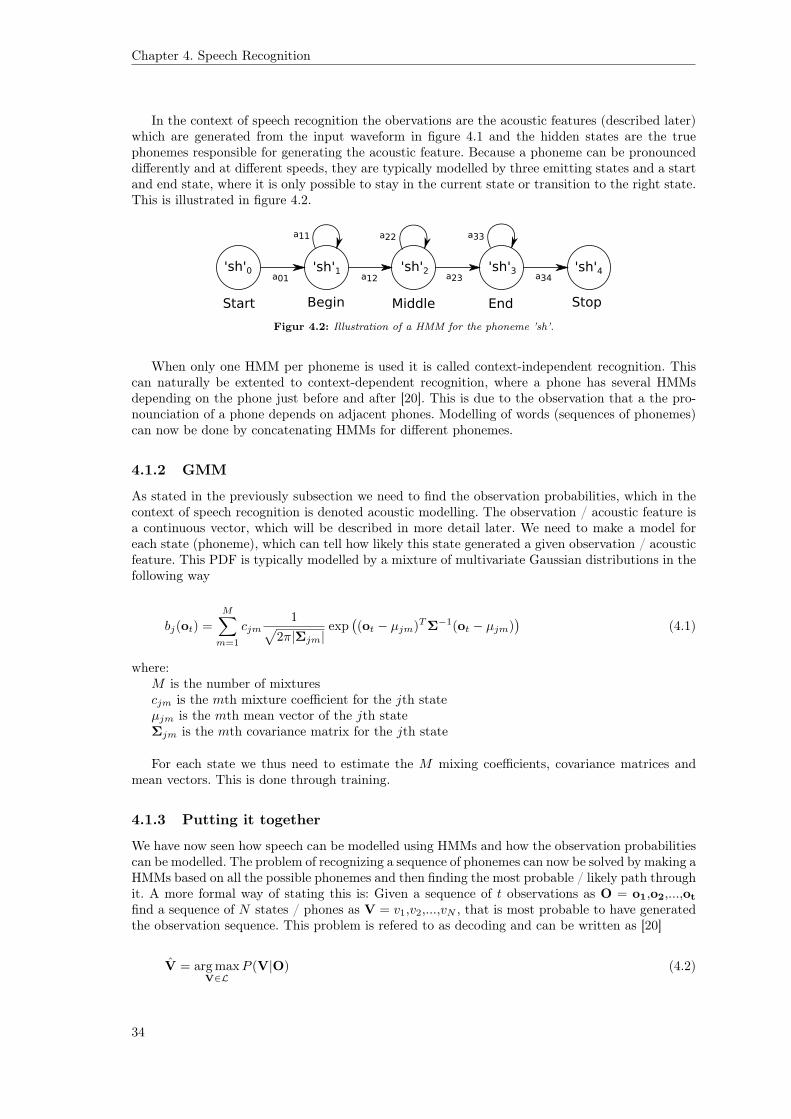
In the context of speech recognition the obervations are the acoustic features (described later)which are generated from the input waveform in figure 4.1 and the hidden states are the truephonemes responsible for generating the acoustic feature. Because a phoneme can be pronounceddifferently and at different speeds, they are typically modelled by three emitting states and a startand end state, where it is only possible to stay in the current state or transition to the right state.This is illustrated in figure 4.2.
'sh'1 'sh'2 'sh'3'sh'0 'sh'4
Begin Middle EndStart Stop
a01
a11
a12
a22
a23
a33
a34
Figur 4.2: Illustration of a HMM for the phoneme ’sh’.
When only one HMM per phoneme is used it is called context-independent recognition. Thiscan naturally be extented to context-dependent recognition, where a phone has several HMMsdepending on the phone just before and after [20]. This is due to the observation that a the pro-nounciation of a phone depends on adjacent phones. Modelling of words (sequences of phonemes)can now be done by concatenating HMMs for different phonemes.
4.1.2 GMM
As stated in the previously subsection we need to find the observation probabilities, which in thecontext of speech recognition is denoted acoustic modelling. The observation / acoustic feature isa continuous vector, which will be described in more detail later. We need to make a model foreach state (phoneme), which can tell how likely this state generated a given observation / acousticfeature. This PDF is typically modelled by a mixture of multivariate Gaussian distributions in thefollowing way
bj(ot) =
M∑m=1
cjm1√
2π|Σjm|exp
((ot − µjm)TΣ−1(ot − µjm)
)(4.1)
where:M is the number of mixturescjm is the mth mixture coefficient for the jth stateµjm is the mth mean vector of the jth stateΣjm is the mth covariance matrix for the jth state
For each state we thus need to estimate the M mixing coefficients, covariance matrices andmean vectors. This is done through training.
4.1.3 Putting it together
We have now seen how speech can be modelled using HMMs and how the observation probabilitiescan be modelled. The problem of recognizing a sequence of phonemes can now be solved by making aHMMs based on all the possible phonemes and then finding the most probable / likely path throughit. A more formal way of stating this is: Given a sequence of t observations as O = o1,o2,...,ot
find a sequence of N states / phones as V = v1,v2,...,vN , that is most probable to have generatedthe observation sequence. This problem is refered to as decoding and can be written as [20]
V = arg maxV∈L
P (V|O) (4.2)
34
Section 4.2. Features
where:L is the set of all possible sequences of states / phonemes
Equation 4.2 can be restated in the following way by using Bayes’ well-known rule
V = arg maxV∈L
P (O|V)P (V)
P (O)= arg max
V∈LP (O|V)P (V) (4.3)
We see in equation 4.3 that the denominator can be dropped since this is constant for all possibleV. We see that P (V) are the transition probabilities mentioned earlier, which is called the languagemodel in the context of speech recognition. The likelihoods, P (O|W) can be computed using thetrained acoustic models in equation 4.1. Since all possible sequences of states/phonemes have tobe evaluated it is necessary to do this efficient. This is achieved by using the Viterbi algorithm[19].
4.2 Features
As depicted in figure 4.1 the input to an ASR system is an acoustic waveform. This waveform hasto be split into features such that the HMM topology can be applied. The most popular featuresare called Mel-Frequency Cepstrum Coefficients (MFCCs) and is computed using the followingsteps [21, 22]
Pre-emphasis A high-pass filter is applied to put emphasis on higher frequencies.
Windowing A window is applied to split the waveform into frames with a typical duration of25ms and an overlap of 10ms. A non-rectangular window is often chosen to avoid problemwhen transforming to frequency domain.
DFT Transforms the time frame into frequency domain.
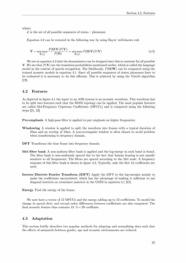
Mel filter bank A non-uniform filter bank is applied and the log-energy in each band is found.The filter bank is non-uniformly spaced due to the fact that human hearing is not equallysensitive to all frequencies. The filters are spaced according to the Mel scale. A frequencyresponse of this filter bank is shown in figure 4.3. Typically, only the first 12 coefficients areused.
Inverse Discrete Fourier Transform (iDFT) Apply the iDFT to the log-energies mainly tomake the coefficients uncorrelated, which has the advantage of making it sufficient to usediagonal matrices as covariance matrices in the GMM in equation 4.1 [21].
Energy Find the energy of the frame.
We now have a vector of 12 MFCCs and the energy adding up to 13 coefficients. To model thechange in speech first- and second order differences between coefficients are also computed. Thefinal acoustic feature thus contains 13 · 3 = 39 coeffients.
4.3 Adaptation
This section briefly describes two popular methods for adapting and normalising data such thatthe effects of mismatch between gender, age and acoustic environments are reduced.
35
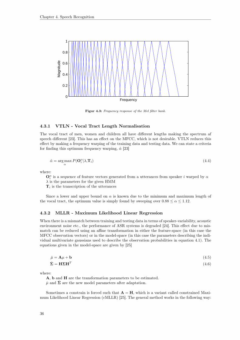
Chapter 4. Speech Recognition
0
0.2
0.4
0.6
0.8
1
Frequency
Mag
nitu
de
Figur 4.3: Frequency response of the Mel filter bank.
4.3.1 VTLN - Vocal Tract Length Normalisation
The vocal tract of men, women and children all have different lengths making the spectrum afspeech different [23]. This has an effect on the MFCC, which is not desirable. VTLN reduces thiseffect by making a frequency warping of the training data and testing data. We can state a criteriafor finding this optimum frequency warping, α [23]
α = arg maxα
P (Oαi |λ,Ti) (4.4)
where:Oαi is a sequence of feature vectors generated from a utterances from speaker i warped by α
λ is the parameters for the given HMMTi is the transcription of the utterances
Since a lower and upper bound on α is known due to the minimum and maximum length ofthe vocal tract, the optimum value is simply found by sweeping over 0.88 ≤ α ≤ 1.12.
4.3.2 MLLR - Maximum Likelihood Linear Regression
When there is a mismatch between training and testing data in terms of speaker-variability, acousticenvironment noise etc., the performance of ASR systems is degraded [24]. This effect due to mis-match can be reduced using an affine transformation in either the feature-space (in this case theMFCC observation vectors) or in the model-space (in this case the parameters describing the indi-vidual multivariate gaussians used to describe the observation probabilities in equation 4.1). Theequations given in the model-space are given by [25]
µ = Aµ+ b (4.5)
Σ = HΣHT (4.6)
where:A, b and H are the transformation parameters to be estimated.µ and Σ are the new model parameters after adaptation.
Sometimes a constrain is forced such that A = H, which is a variant called constrained Maxi-mum Likelihood Linear Regression (cMLLR) [25]. The general method works in the following way:
36
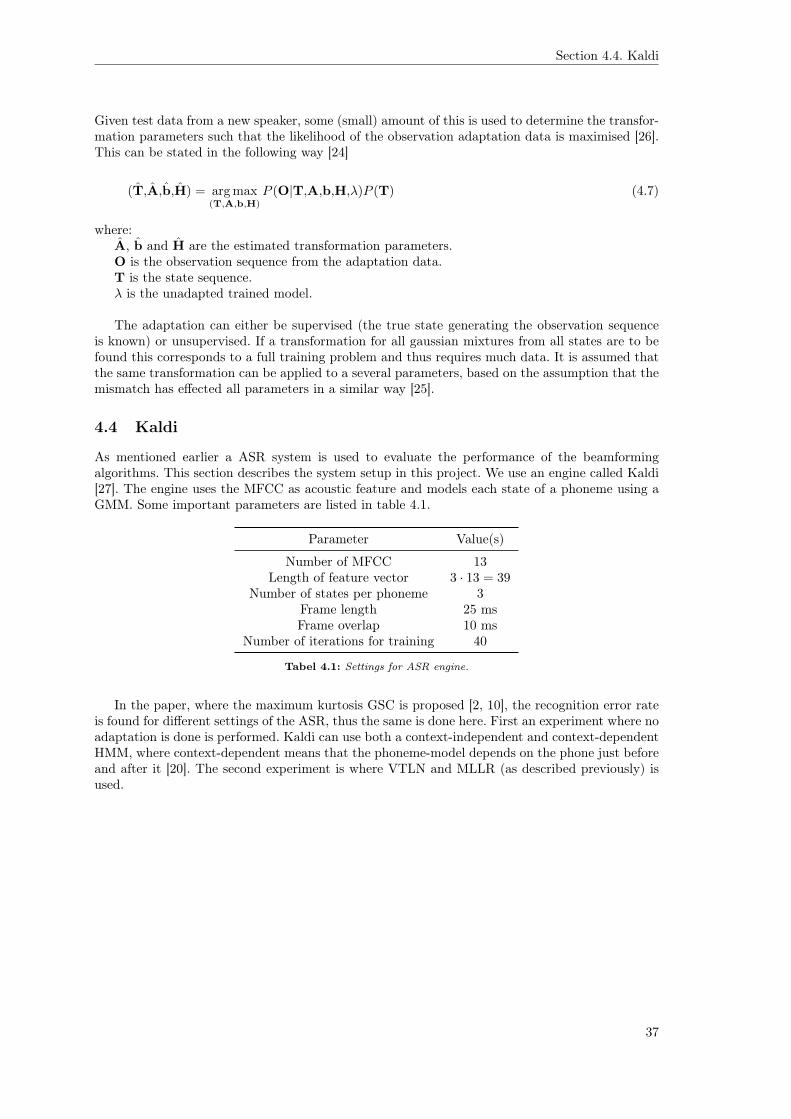
Section 4.4. Kaldi
Given test data from a new speaker, some (small) amount of this is used to determine the transfor-mation parameters such that the likelihood of the observation adaptation data is maximised [26].This can be stated in the following way [24]
(T,A,b,H) = arg max(T,A,b,H)
P (O|T,A,b,H,λ)P (T) (4.7)
where:A, b and H are the estimated transformation parameters.O is the observation sequence from the adaptation data.T is the state sequence.λ is the unadapted trained model.
The adaptation can either be supervised (the true state generating the observation sequenceis known) or unsupervised. If a transformation for all gaussian mixtures from all states are to befound this corresponds to a full training problem and thus requires much data. It is assumed thatthe same transformation can be applied to a several parameters, based on the assumption that themismatch has effected all parameters in a similar way [25].
4.4 Kaldi
As mentioned earlier a ASR system is used to evaluate the performance of the beamformingalgorithms. This section describes the system setup in this project. We use an engine called Kaldi[27]. The engine uses the MFCC as acoustic feature and models each state of a phoneme using aGMM. Some important parameters are listed in table 4.1.
Parameter Value(s)
Number of MFCC 13Length of feature vector 3 · 13 = 39
Number of states per phoneme 3Frame length 25 msFrame overlap 10 ms
Number of iterations for training 40
Tabel 4.1: Settings for ASR engine.
In the paper, where the maximum kurtosis GSC is proposed [2, 10], the recognition error rateis found for different settings of the ASR, thus the same is done here. First an experiment where noadaptation is done is performed. Kaldi can use both a context-independent and context-dependentHMM, where context-dependent means that the phoneme-model depends on the phone just beforeand after it [20]. The second experiment is where VTLN and MLLR (as described previously) isused.
37
Chapter 5. Experimental Results
Kapitel 5
Experimental Results
To show an improvement using the GSC with kurtosis criteria the algorithm is tested in terms ofPER for different acoustic environments. This chapter is dedicated to describing the data used,stating the results and finally discuss and compare them with results achieved in other projects.
5.1 Data
The purpose of this section is to describe the data used to benchmark the performance of thearray processing algorithms. In both the synthetic case and the real-world case we use data fromthe well-known TIMIT database. Appendix E lists the 16 sentences used which makes a total of610 phonemes to be recognised. This is considered enough to show a performance gain if any.The synthetic reverberation is generated using a MATLAB implementation made by [28], whichbasically uses the image-source model to generate the desired Room Impulse Response (RIR) andthen convolves this with the 16 TIMIT sentences in appendix E on page 56. Table 5.1 shows thesettings for generating the synthetic data, where xM refers to the position of the center of themicrophone array.
Parameter Value(s)
Room dimension [x,y,z] [3, 4, 2.5]xM [x,y,z] [1.5, 1, 1.3]xS [x,y,z] [1.5, 2.5, 1.5]
Incident angle 90°
Tabel 5.1: Room settings for generating synthetic data.
The real-world data was captured at in the spring 2013 at UT Dallas, Texas. It was generatedby having a speaker read the aforementioned TIMIT sentences in two rooms with different acousticcharacteristica, while recording with a microphone array and a single microphone attached close tothe speaker’s mouth. Images and drawings of the rooms are shown in appendix F along with a tableshowing dimensions of the rooms, location of the speaker and microphone array. The microphonearray used for recording has the same geometry as the one used to generate synthetic data.
5.2 Results
This section states the results achieved by applying the maximum kurtosis GSC on the datadescribed in the previously section, and then comparing with the very simple DSB, as this seemsto be the general approach. The PER for the clean speech and raw distant microphone are alsostated. Table 5.2 shows how the beamformers are abbreviated in the rest of this chapter.
As mentioned in 4 there are context-independent and -dependent HMM modelling and furt-hermore different adaptation methods which can be applied in order to increase performance ofthe ASR system. Because of this three PERs are given for each method. We denote them in thefollowing way: Context-independent recognition is denoted MONO, context-dependent recognition
38
Section 5.2. Results
Signal Abbreviation
Clean data CLEANSingle-channel reverberant data from center microphone of microphone array RAWDelay-and-sum beamformer DSBDelay-and-sum beamformer + Zelinski postfiltering DSB-PFGSC with Kurtosis criteria GSC-KGSC with Kurtosis criteria + Zelinski postfiltering GSC-K-PFGSC with Kurtosis criteria and subspace filtering GSC-K-SPGSC with Kurtosis criteria and subspace filtering + Zelinski postfiltering GSC-K-SP-PF
Tabel 5.2: Table of abbreviations
is denoted TRI and context-dependent recognition with VTLN and MLLR is denoted VTLN &MLLR. Besides using only the PER, histograms and spectrograms are also shown for selectedsettings. When looking at the gradient of the cost function given in equation 3.27 in section 3.3.2we see that for a signal with range in amplitude the two first terms might be very small. Becauseof this a sufficent high step size should be chosen. Also it is therefore very important that alphais not set too high forcing w to become all zeros. The parameters are found imperically on datanot in the test set. The gradient method used to find the optimum filter weights is terminatedwhen the kurtosis of the output has converged. Through initial experiments so change was seenusing the contribution ratio described in equation 3.34, so when testing with subspace filter thedimension of the signal space is fixed to 2.
5.2.1 Synthetic data
Two different types of experiments are conducted; First where the block size used to estimate thefilter weights is fixed and the reverberation time is varied along with different SNRs, and secondwhere the reverberation time is fixed and the block size is varied. In the first experiment the twoSNRs are chosen to be 20dB and 60dB, and the case of varying block size SNR is set to 60dB.
Different reverberation timesTable 5.3, 5.4 and 5.5 show the ASR results obtained for a reverberation time of 0.1s, 0.3s and0.5s, respectively. It is first noted that even a low reverberation time of 0.1s degrades performancedramatically and that a reverberation time of 0.5s doubles the PER. As an overall trend, both theDSB and maximum kurtosis GSC increase performance for all three settings of the ASR systemsignificantly. When comparing the DSB and the maximum kurtosis GSC, the first performs thebest in all cases when postfiltering is not considered. When comparing the maximum kurtosis GSCwithout subspace filtering to the one with subspace filtering no difference in performance is seen,however the dimension of the filter is reduced with one dimension but at the cost of calculatingthe sample covariance matrix.
To see how the maximum kurtosis improves the speech signal, spectrograms and histogramsare shown for the case of a reverberation time of 0.5s and a SNR of 60dB. Figure 5.1 shows thehistogram and fitted distributions for (a) the clean speech, (b) the raw speech and (c) the outputfrom the maximum kurtosis GSC. We clearly see that the clean speech is peaky and has heavytails, which is best modelled by a gamma distribution, whereas the raw speech is better modelledas a laplace distribution as we also saw in section 3.3.2. The output of the maximum kurtosis GSCis best fitted by a gamma distribution, which indicates that the algorithm has improved this aspectas expected.
Figure 5.2 shows the spectrogram for (a) the clean speech, (b) the raw speech, (c) the outputfrom maximum kurtosis GSC and (d) the output from the maximum kurtosis GSC with postfilte-ring. We first note the degradation of the from the clean speech to the raw speech and the effect ofthe reverberation is clearly seen. When comparing the raw speech with the output from the maxi-mum kurtosis GSC we do see an improvement and that some reverberation has been decreased,
39
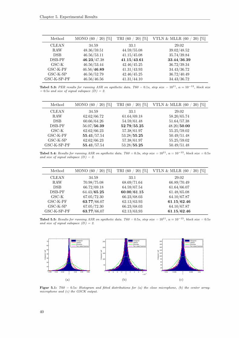
Chapter 5. Experimental Results
Method MONO (60 / 20) [%] TRI (60 / 20) [%] VTLN & MLLR (60 / 20) [%]
CLEAN 34.59 33.1 29.02RAW 48.36/59.51 44.59/55.08 39.02/48.52DSB 46.56/53.11 41.15/45.08 35.74/39.84
DSB-PF 46.23/47.38 41.15/43.61 33.44/36.39GSC-K 46.56/53.44 42.46/45.25 36.72/39.34
GSC-K-PF 46.56/46.89 41.31/43.93 34.43/36.72GSC-K-SP 46.56/52.79 42.46/45.25 36.72/40.49
GSC-K-SP-PF 46.56/46.56 41.31/44.10 34.43/36.72
Tabel 5.3: PER results for running ASR on synthetic data. T60 = 0.1s, step size = 1011, α = 10−13, block size= 0.5s and size of signal subspace (D) = 2.
Method MONO (60 / 20) [%] TRI (60 / 20) [%] VTLN & MLLR (60 / 20) [%]
CLEAN 34.59 33.1 29.02RAW 62.62/66.72 61.64/69.18 58.20/65.74DSB 60.66/64.26 54.59/61.48 51.64/57.38
DSB-PF 56.07/56.39 52.79/55.25 48.20/50.00GSC-K 62.62/66.23 57.38/61.97 55.25/59.02
GSC-K-PF 55.41/57.54 53.28/55.25 50.49/51.48GSC-K-SP 62.62/66.23 57.38/61.97 55.25/59.02
GSC-K-SP-PF 55.41/57.54 53.28/55.25 50.49/51.48
Tabel 5.4: Results for running ASR on synthetic data. T60 = 0.3s, step size = 1011, α = 10−13, block size = 0.5sand size of signal subspace (D) = 2.
Method MONO (60 / 20) [%] TRI (60 / 20) [%] VTLN & MLLR (60 / 20) [%]
CLEAN 34.59 33.1 29.02RAW 70.98/75.08 68.69/71.64 66.89/70.49DSB 66.72/69.18 64.59/67.54 61.64/66.07
DSB-PF 64.43/65.25 60.00/61.15 61.48/65.08GSC-K 67.05/72.30 66.23/68.03 64.10/67.87
GSC-K-PF 63.77/66.07 62.13/63.93 61.15/62.46GSC-K-SP 67.05/72.30 66.23/68.03 64.10/67.87
GSC-K-SP-PF 63,77/66,07 62.13/63,93 61.15/62.46
Tabel 5.5: Results for running ASR on synthetic data. T60 = 0.5s, step size = 1011, α = 10−13, block size = 0.5sand size of signal subspace (D) = 2.
−0.06 −0.04 −0.02 0 0.02 0.04 0.060
10
20
30
40
50
60
70
x
His
togr
am /
HistogramLaplaceGaussianTwo−sided Gamma
(a)
−8 −6 −4 −2 0 2 4 6 8
x 10−3
0
50
100
150
200
250
x
His
togr
am /
HistogramLaplaceGaussianTwo−sided Gamma
(b)
−0.01 −0.005 0 0.005 0.010
20
40
60
80
100
120
140
160
180
200
x
His
togr
am /
HistogramLaplaceGaussianTwo−sided Gamma
(c)
Figur 5.1: T60 = 0.5s: Histogram and fitted distributions for (a) the close microphone, (b) the center array-microphone and (c) the GSCK output.
40
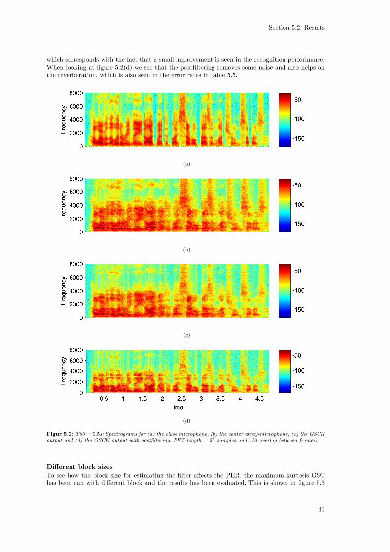
Section 5.2. Results
which corresponds with the fact that a small improvement is seen in the recognition performance.When looking at figure 5.2(d) we see that the postfiltering removes some noise and also helps onthe reverberation, which is also seen in the error rates in table 5.5.
(a)
(b)
(c)
(d)
Figur 5.2: T60 = 0.5s: Spectrograms for (a) the close microphone, (b) the center array-microphone, (c) the GSCKoutput and (d) the GSCK output with postfiltering. FFT-length = 28 samples and 1/8 overlap between frames.
Different block sizesTo see how the block size for estimating the filter affects the PER, the maximum kurtosis GSChas been run with different block and the results has been evaluated. This is shown in figure 5.3
41
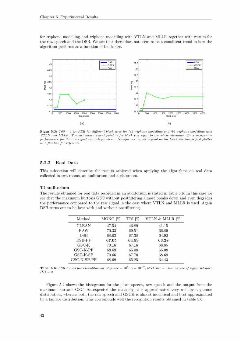
Chapter 5. Experimental Results
for triphone modelling and triphone modelling with VTLN and MLLR together with results forthe raw speech and the DSB. We see that there does not seem to be a consistent trend in how thealgorithm performs as a function of block size.
0 500 1000 1500 2000 2500 3000 3500 400041
41.5
42
42.5
43
43.5
44
44.5
45
Block size
PE
R [%
]
DSBGSCKRaw
(a)
0 500 1000 1500 2000 2500 3000 3500 400035.5
36
36.5
37
37.5
38
38.5
39
39.5
Block size
PE
R [%
]
DSBGSCKRaw
(b)
Figur 5.3: T60 = 0.1s: PER for different block sizes for (a) triphone modelling and (b) triphone modelling withVTLN and MLLR. The last measurement point is for block size equal to the whole utterance. Since recognitionperformance for the raw signal and delay-and-sum beamformer do not depend on the block size this is just plottedas a flat line for reference.
5.2.2 Real Data
This subsection will describe the results achieved when applying the algorithms on real datacollected in two rooms, an auditorium and a classroom.
TI-auditoriumThe results obtained for real data recorded in an auditorium is stated in table 5.6. In this case wesee that the maximum kurtosis GSC without postfiltering almost breaks down and even degradesthe performance compared to the raw signal in the case where VTLN and MLLR is used. AgainDSB turns out to be best with and without postfiltering.
Method MONO [%] TRI [%] VTLN & MLLR [%]
CLEAN 47.54 46.89 41.15RAW 70.33 69.51 66.89DSB 68.03 67.38 64.92
DSB-PF 67.05 64.59 63.28GSC-K 70.16 67.16 68.85
GSC-K-PF 68.69 65.08 65.08GSC-K-SP 70.66 67.70 68.69
GSC-K-SP-PF 68.69 65.25 64.43
Tabel 5.6: ASR results for TI-auditorium. step size = 105, α = 10−7, block size = 0.5s and size of signal subspace(D) = 2.
Figure 5.4 shows the histograms for the clean speech, raw speech and the output from themaximum kurtosis GSC. As expected the clean signal is approximated very well by a gammedistribution, whereas both the raw speech and GSCK is almost indentical and best approximatedby a laplace distribution. This corresponds well the recognition results obtained in table 5.6.
42
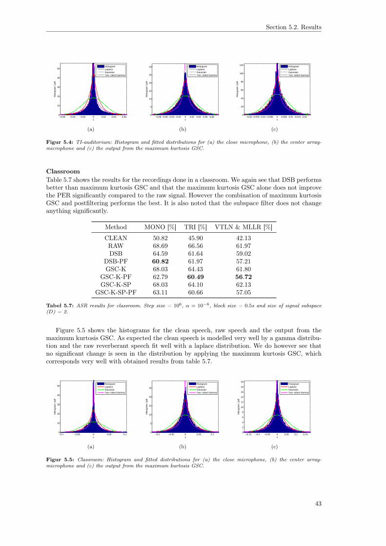
Section 5.2. Results
−0.06 −0.04 −0.02 0 0.02 0.04 0.060
10
20
30
40
50
x
His
togr
am /
HistogramLaplaceGaussianTwo−sided Gamma
(a)
−0.08 −0.06 −0.04 −0.02 0 0.02 0.04 0.06 0.080
5
10
15
20
25
30
x
His
togr
am /
HistogramLaplaceGaussianTwo−sided Gamma
(b)
−0.02 −0.015 −0.01 −0.005 0 0.005 0.01 0.015 0.020
20
40
60
80
100
120
x
His
togr
am /
HistogramLaplaceGaussianTwo−sided Gamma
(c)
Figur 5.4: TI-auditorium: Histogram and fitted distributions for (a) the close microphone, (b) the center array-microphone and (c) the output from the maximum kurtosis GSC.
ClassroomTable 5.7 shows the results for the recordings done in a classroom. We again see that DSB performsbetter than maximum kurtosis GSC and that the maximum kurtosis GSC alone does not improvethe PER significantly compared to the raw signal. However the combination of maximum kurtosisGSC and postfiltering performs the best. It is also noted that the subspace filter does not changeanything significantly.
Method MONO [%] TRI [%] VTLN & MLLR [%]
CLEAN 50.82 45.90 42.13RAW 68.69 66.56 61.97DSB 64.59 61.64 59.02
DSB-PF 60.82 61.97 57.21GSC-K 68.03 64.43 61.80
GSC-K-PF 62.79 60.49 56.72GSC-K-SP 68.03 64.10 62.13
GSC-K-SP-PF 63.11 60.66 57.05
Tabel 5.7: ASR results for classroom. Step size = 106, α = 10−6, block size = 0.5s and size of signal subspace(D) = 2.
Figure 5.5 shows the histograms for the clean speech, raw speech and the output from themaximum kurtosis GSC. As expected the clean speech is modelled very well by a gamma distribu-tion and the raw reverberant speech fit well with a laplace distribution. We do however see thatno significant change is seen in the distribution by applying the maximum kurtosis GSC, whichcorresponds very well with obtained results from table 5.7.
−0.1 −0.05 0 0.05 0.10
10
20
30
40
50
x
His
togr
am /
HistogramLaplaceGaussianTwo−sided Gamma
(a)
−0.1 −0.05 0 0.05 0.10
5
10
15
20
25
x
His
togr
am /
HistogramLaplaceGaussianTwo−sided Gamma
(b)
−0.15 −0.1 −0.05 0 0.05 0.1 0.150
2
4
6
8
10
12
14
16
18
20
x
His
togr
am /
HistogramLaplaceGaussianTwo−sided Gamma
(c)
Figur 5.5: Classroom: Histogram and fitted distributions for (a) the close microphone, (b) the center array-microphone and (c) the output from the maximum kurtosis GSC.
43
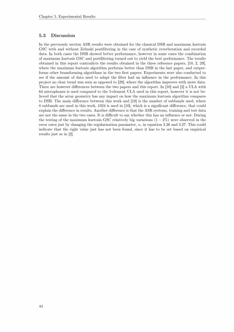
Chapter 5. Experimental Results
5.3 Discussion
In the previously section ASR results were obtained for the classical DSB and maximum kurtosisGSC with and without Zelinski postfiltering in the case of synthetic reverberation and recordeddata. In both cases the DSB showed better performance, however in some cases the combinationof maximum kurtosis GSC and postfiltering turned out to yield the best performance. The resultsobtained in this report contradicts the results obtained in the three reference papers, [10, 2, 29],where the maximum kurtosis algorithm performs better than DSB in the last paper, and outper-forms other beamforming algorithms in the two first papers. Experiments were also conducted tosee if the amount of data used to adapt the filter had an influence in the performance. In thisproject no clear trend was seen as opposed to [29], where the algorithm improves with more data.There are however differences between the two papers and this report. In [10] and [2] a ULA with64 microphones is used compared to the 5-element ULA used in this report, however it is not be-lieved that the array geometry has any impact on how the maximum kurtosis algorithm comparesto DSB. The main difference between this work and [10] is the number of subbands used, where8 subbands are used in this work, 1024 is used in [10], which is a significant difference, that couldexplain the difference in results. Another difference is that the ASR systems, training and test dataare not the same in the two cases. It is difficult to say whether this has an influence or not. Duringthe testing of the maximum kurtosis GSC relatively big variations (1− 2%) were observed in theerror rates just by changing the regularization parameter, α, in equation 3.26 and 3.27. This couldindicate that the right value just has not been found, since it has to be set based on empiricalresults just as in [2].
44
Chapter 6. Conclusion
Kapitel 6
Conclusion
This project has concerned the use of array processing to improve speech recognition in scenarioswhere reverberation is a significant problem. A reverberant signal model for a microphone array wasstated along with some important statistical properties. Focus was naroowed down to investigatethe proposed beamforming algorithm method in [10, 2]. The method is an extended version of thewell-known GSC beamforming algorithm, where kurtosis is used as an optimization criteria, basedon the observation that clean speech has a higher kurtosis than reverberant speech due to the CLT.This observation was confirmed by using histograms of clean and reverberant speech. A similarsystem as in [10, 2, 29] was implemented and each block was verified. The recognition softwareKaldi was set up such that the algorithm could be benchmarked against the classic DSB andthe general theory of HMM speech recognition was presented along with two popular adaptationmethods, namely VTLN and MLLR. As test data both synthetic data and real recorded data wasused. The method improved the recognition performance in almost all cases compared to the rawsignal, but did not perform better than DSB. This contradicts with the results stated in [10, 2],where the method achieves good results compared to other beamforming algorithms. The maindifference between the work in this project and the reference papers is the number of frequencysubbands used. This will be investigated further to determine if this is the cause of the poorperformance. The results also showed that Zelinski posfiltering had a positive effect on reducingthe PER in almost all cases.
45


References
[1] J. McDonough and M. Wölfel, Distant Speech Recognition. John Wiley & Sons, Inc., 2009.
[2] K. Kumatani, J. McDonough, and B. Raj, “Maximum kurtosis beamforming with a subspacefilter for distant speech recognition,” in Automatic Speech Recognition and Understanding(ASRU), 2011 IEEE Workshop on, dec. 2011, pp. 179 –184.
[3] P. A. Naylor and N. D. Gaubitch, Speech Dereverberation. Springer, 2010.
[4] J. Benesty, J. Chen, and Y. Huang, Microphone Array Signal Processing. Springer, 2008.
[5] E. A. P. Habets, “Single- and multi-microphone speech dereverberation using spectral enhan-cement,” Ph.D. dissertation, Eindhoven University of Technology, 2007.
[6] S. Haykin, Adaptive Filter Theory, 3rd ed. Prentice Hall, 2002.
[7] H. Krim and M. Viberg, “Two decades of array signal processing research,” IEEE SignalProcessing Magazine, jul 1996.
[8] H. L. V. Trees, Optimum Array Processing. Part IV of Detection, Estimation and ModulationTheory. Wiley, 2002.
[9] B. Widrow, K. Duvall, R. Gooch, andW. Newman, “Signal cancellation phenomena in adaptiveantennas: Causes and cures,” Antennas and Propagation, IEEE Transactions on, vol. 30, no. 3,pp. 469 – 478, may 1982.
[10] K. Kumatani, J. McDonough, and B. Raj, “Block-wise incremental adaptation algorithm formaximum kurtosis beamforming,” in Applications of Signal Processing to Audio and Acoustics(WASPAA), 2011 IEEE Workshop on, 2011, pp. 229–232.
[11] P. P. Vaidyanathan, Multirate Systems and Filter Banks. Prentice Hall, 1993.
[12] A. Hyvärinen, J. Karhunen, and E. Oja, Independent Component Analysis, 1st ed. JohnWiley & Sons, Inc., 2001.
[13] T. Petsatodis, C. Boukis, F. Talantzis, Z.-H. Tan, and R. Prasad, “Convex combination ofmultiple statistical models with application to vad,” Audio, Speech, and Language Processing,IEEE Transactions on, vol. 19, no. 8, pp. 2314 –2327, nov 2011.
[14] S. Boyd and L. Vandenberghe, Convex Optimization. Cambridge University Press, 2004.
[15] P. Stoica and R. Moses, Introduction to Spectral Analysis. Prentice Hall, 1997.
[16] D. H. Johnson and D. E. Dudgeon, Array Signal Processing - Concepts and Techniques, 1st ed.Prentice Hall, 1993.
[17] S. Kay, Intuitive Probability and Random Processes using MATLAB, 1st ed. Springer, 2006.
[18] R. Zelinski, “A microphone array with adaptive post-filtering for noise reduction in reverberantrooms,” in Acoustics, Speech, and Signal Processing, 1988. ICASSP-88., 1988 InternationalConference on, apr 1988, pp. 2578 –2581 vol.5.
47
References
[19] L. Rabiner, “A tutorial on hidden markov models and selected applications in speech recog-nition,” Proceedings of the IEEE, vol. 77, no. 2, pp. 257–286, 1989.
[20] K.-F. Lee and H.-W. Hon, “Speaker-independent phone recognition using hidden markov mo-dels,” Acoustics, Speech and Signal Processing, IEEE Transactions on, vol. 37, no. 11, pp.1641–1648, 1989.
[21] C. Becchetti and L. P. Ricotti, Speech Recognition - Theory and C++ Implementation. JohnWiley & Sons, Inc., 2009.
[22] J. R. Deller, J. H. L. Hansen, and J. G. Proakis, Discrete-Time Processing of Speech Signals.Wiley - Interscience, 2000.
[23] L. Lee and R. Rose, “Speaker normalization using efficient frequency warping procedures,” inAcoustics, Speech, and Signal Processing, 1996. ICASSP-96. Conference Proceedings., 1996IEEE International Conference on, vol. 1, 1996, pp. 353–356 vol. 1.
[24] A. Sankar and C.-H. Lee, “A maximum-likelihood approach to stochastic matching for robustspeech recognition,” Speech and Audio Processing, IEEE Transactions on, vol. 4, no. 3, pp.190–202, 1996.
[25] M. Gales, “Maximum likelihood linear transformations for hmm-based speech recognition,”Computer Speech and Language, vol. 12, pp. 75–98, 1998.
[26] C. Leggetter and P. Woodland, “Maximum likelihood linear regression for speaker adaptationof continuous density hidden markov models,” Computer Speech & Language, vol. 9, no. 2,pp. 171 – 185, 1995. [Online]. Available: http://www.sciencedirect.com/science/article/pii/S0885230885700101
[27] D. Povey, A. Ghoshal, G. Boulianne, L. Burget, O. Glembek, N. Goel, M. Hannemann, P. Mot-licek, Y. Qian, P. Schwarz, J. Silovsky, G. Stemmer, and K. Vesely, “The kaldi speech recogni-tion toolkit,” in IEEE 2011 Workshop on Automatic Speech Recognition and Understanding.IEEE Signal Processing Society, dec 2011, IEEE Catalog No.: CFP11SRW-USB.
[28] E. Lehmann and A. Johansson, “Diffuse reverberation model for efficient image-source simula-tion of room impulse responses,” Audio, Speech, and Language Processing, IEEE Transactionson, vol. 18, no. 6, pp. 1429–1439, 2010.
[29] K. Kumatani, J. Mcdonough, B. Rauch, P. N. Garner, W. Li, and J. Dines, “Maximum kurtosisbeamforming with the generalized sidelobe canceller.”
[30] C. H. Edwards and D. E. Penney, Calculus Early Transcendentals, 7th ed. Prentice Hall,2008.
48

Appendix
49

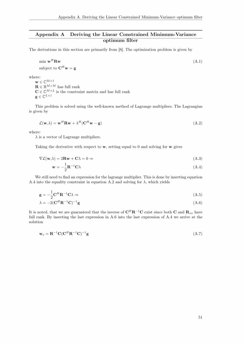
Appendix A. Deriving the Linear Constrained Minimum-Variance optimum filter
Appendix A Deriving the Linear Constrained Minimum-Varianceoptimum filter
The derivations in this section are primarily from [8]. The optimization problem is given by
min wHRw (A.1)
subject to CHw = g
where:w ∈ CM×1R ∈ RM×M has full rankC ∈ CM×L is the constraint matrix and has full rankg ∈ CL×1
This problem is solved using the well-known method of Lagrange multipliers. The Lagrangianis given by
L(w,λ) = wHRw + λH(CHw − g) (A.2)
where:λ is a vector of Lagrange multipliers.
Taking the derivative with respect to w, setting equal to 0 and solving for w gives
∇L(w,λ) = 2Rw + Cλ = 0⇒ (A.3)
w = −1
2R−1Cλ (A.4)
We still need to find an expression for the lagrange multiplier. This is done by inserting equationA.4 into the equality constraint in equation A.2 and solving for λ, which yields
g = −1
2CHR−1Cλ⇒ (A.5)
λ = −2(CHR−1C)−1g (A.6)
It is noted, that we are guaranteed that the inverse of CHR−1C exist since both C and Rxx havefull rank. By inserting the last expression in A.6 into the last expression of A.4 we arrive at thesolution
wo = R−1C(CHR−1C)−1g (A.7)
51
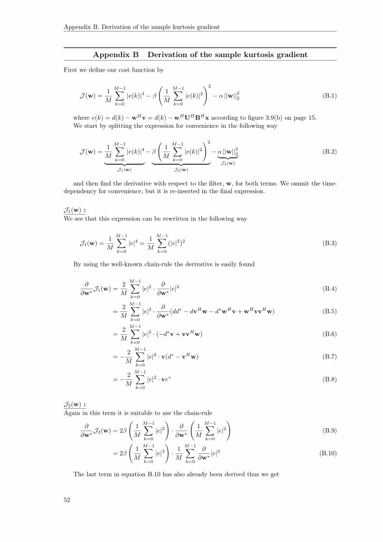
Appendix B. Derivation of the sample kurtosis gradient
Appendix B Derivation of the sample kurtosis gradient
First we define our cost function by
J (w) =1
M
M−1∑k=0
|e(k)|4 − β
(1
M
M−1∑k=0
|e(k)|2)2
− α ||w||22 (B.1)
where e(k) = d(k)−wHv = d(k)−wHUHBHx according to figure 3.9(b) on page 15.We start by splitting the expression for convenience in the following way
J (w) =1
M
M−1∑k=0
|e(k)|4︸ ︷︷ ︸J1(w)
−β
(1
M
M−1∑k=0
|e(k)|2)2
︸ ︷︷ ︸J2(w)
−α ||w||22︸ ︷︷ ︸J3(w)
(B.2)
and then find the derivative with respect to the filter, w, for both terms. We ommit the time-dependency for convenience, but it is re-inserted in the final expression.
J1(w) :We see that this expression can be rewritten in the following way
J1(w) =1
M
M−1∑k=0
|e|4 =1
M
M−1∑k=0
(|e|2)2 (B.3)
By using the well-known chain-rule the derivative is easily found
∂
∂w∗J1(w) =
2
M
M−1∑k=0
|e|2 · ∂
∂w∗|e|2 (B.4)
=2
M
M−1∑k=0
|e|2 · ∂
∂w∗(dd∗ − dvHw − d∗wHv + wHvvHw) (B.5)
=2
M
M−1∑k=0
|e|2 · (−d∗v + vvHw) (B.6)
= − 2
M
M−1∑k=0
|e|2 · v(d∗ − vHw) (B.7)
= − 2
M
M−1∑k=0
|e|2 · ve∗ (B.8)
J2(w) :Again in this term it is suitable to use the chain-rule
∂
∂w∗J2(w) = 2β
(1
M
M−1∑k=0
|e|2)· ∂
∂w∗
(1
M
M−1∑k=0
|e|2)
(B.9)
= 2β
(1
M
M−1∑k=0
|e|2)· 1
M
M−1∑k=0
∂
∂w∗|e|2 (B.10)
The last term in equation B.10 has also already been derived thus we get
52
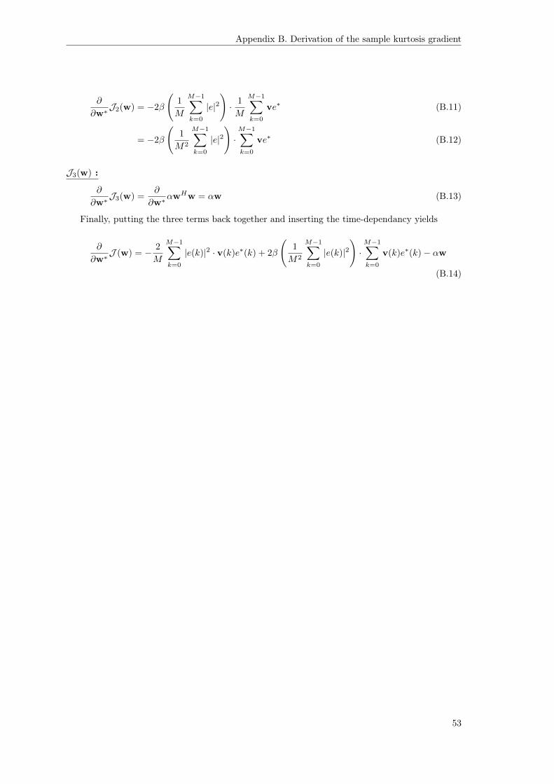
Appendix B. Derivation of the sample kurtosis gradient
∂
∂w∗J2(w) = −2β
(1
M
M−1∑k=0
|e|2)· 1
M
M−1∑k=0
ve∗ (B.11)
= −2β
(1
M2
M−1∑k=0
|e|2)·M−1∑k=0
ve∗ (B.12)
J3(w) :
∂
∂w∗J3(w) =
∂
∂w∗αwHw = αw (B.13)
Finally, putting the three terms back together and inserting the time-dependancy yields
∂
∂w∗J (w) = − 2
M
M−1∑k=0
|e(k)|2 · v(k)e∗(k) + 2β
(1
M2
M−1∑k=0
|e(k)|2)·M−1∑k=0
v(k)e∗(k)− αw
(B.14)
53
Appendix C. Kurtosis of random variable with standard normal distribution
Appendix C Kurtosis of random variable with standard normaldistribution
This aims to show that the kurtosis of a random variable with standard normal distribution iszero, i.e.
Kurt(X) = E[X4]− 3E[X2]2 = 0, for fX(x) =1√2πe
−x22 (C.1)
where:fX(x) is the PDF of the random variable X
Due to the assumption of unit variance, the expression becomesKurt(X) = E[X4]− 3 = 0; (C.2)
We thus need to show that E[X4] = 3.
E[X4] =
∫ ∞−∞
x4fX(x) dx (C.3)
=1√2π
∫ ∞−∞
x4e−x22 dx (C.4)
The method of integration by parts, which states that∫udv = uv −
∫vdu, can now be used
[30, p. 521]. Setting
u = x3 → du = 3x2dx (C.5)
dv = xe−x22 → v = −e
−x22 (C.6)
We thus get
E[X4] =1√2π
∫ ∞−∞
x4e−x22 dx (C.7)
=1√2π
(−x3e
−x22 −
∫ ∞−∞−e
−x22 3x2dx
)(C.8)
=1√2π
(−x3e
−x22 + 3
∫ ∞−∞
e−x22 x2dx
)(C.9)
=1√2π
([−x3e
−x22 + 3 ·
(√π
2erf(x√2
)− xe
−x22
)]∞−∞
)(C.10)
We clearly see that the exponentials evaluate to zero for plus and minus infinity, i.e. e−x22 = 0|±∞.
We are thus left with
E[X4] =3√2π
[√π
2erf(x√2
)]∞−∞
(C.11)
=3√2π
√π
2
(erf(∞√
2
)− erf
(−∞√
2
))(C.12)
=3√2π
√π
2(1− (−1)) (C.13)
=3√
2√π·√π√2· 2 (C.14)
= 3 (C.15)
We thus have that Kurt(X) = E[X4]− 3 = 3− 3 = 0.
54
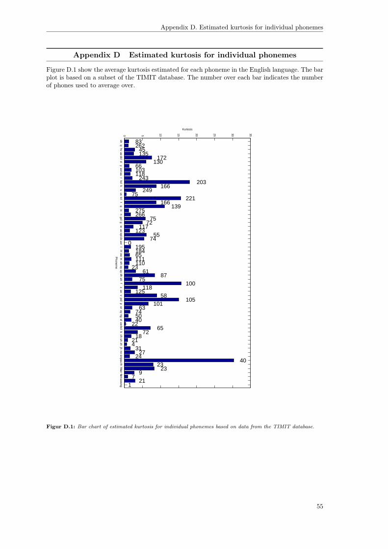
Appendix D. Estimated kurtosis for individual phonemes
Appendix D Estimated kurtosis for individual phonemes
Figure D.1 show the average kurtosis estimated for each phoneme in the English language. The barplot is based on a subset of the TIMIT database. The number over each bar indicates the numberof phones used to average over.
shiy
hvae
dcld
yaxraa
rkcl
ks
uxtcl
tq
ixn
gclg
wao
epidxaxr
lih
owm
ehoy
aydh
ahf
zax
vpcl
per
eyng
eluw
bclb
chuh
zhjh
nxen
pauth
hhax−hem
aweng
0 5 10 15 20 25 30 35
Phonem
e
Kurtosis
83262
45135
172130
66103118
243203
166249
75221
166139
275266
7572
117123
5574
019518465111110
2361
8775
100118
12558
105101
63745040
2265
7218
214
3127
2440
2323
97
211
Figur D.1: Bar chart of estimated kurtosis for individual phonemes based on data from the TIMIT database.
55

Appendix E. TIMIT sentences
Appendix E TIMIT sentences
DR1 - MDAB0• He has never, himself, done anything for which to be hated - which of us has?
• Be excited and don’t identify yourself.
• Sometimes, he coincided with my father’s being at home.
• At twilight on the twelfth day we’ll have Chablis.
• The bungalow was pleasantly situated near the shore.
• Are you looking for employment?
• A big goat idly ambled through the farmyard.
• Eating spinach nightly increases strength miraculously.
DR1 - MWBT0• To many experts, this trend was inevitable.
• However, the litter remained, augmented by several dozen lunchroom suppers.
• Books are for schnooks.
• Those musicians harmonize marvelously.
• A muscular abdomen is good for your back.
• The causeway ended abruptly at the shore.
• Please take this dirty table cloth to the cleaners for me.
• The carpet cleaners shampooed our oriental rug.
56
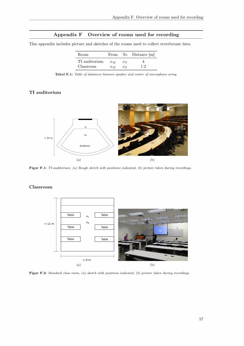
Appendix F. Overview of rooms used for recording
Appendix F Overview of rooms used for recording
This appendix includes picture and sketches of the rooms used to collect reverberant data.
Room From To Distance [m]
TI auditorium xM xS 4Classroom xM xS 1.2
Tabel F.1: Table of distances between speaker and center of microphone array.
TI auditorium
Audience
xs
xM
≈ 25 m
(a) (b)
Figur F.1: TI-auditorium, (a) Rough sketch with positions indicated, (b) picture taken during recordings.
Classroom
Table
Table
Table
Table
Table
Table
xM
xS
≈ 11 m
≈ 9 m
(a) (b)
Figur F.2: Standard class room, (a) sketch with positions indicated, (b) picture taken during recordings.
57