Distance Protection: Why Have We Started With a Circle, Does It Matter, and What Else

Is Out There? Edmund O. Schweitzer, III and Bogdan Kasztenny

Schweitzer Engineering Laboratories, Inc.

Abstract—We look back at the history of distance protection, explain the first principles, and discuss why our industry settled on designs we know and appreciate today. We look at why, after a century of refinements, a typical distance element still uses heavily filtered voltages and currents and operates on the order of one power cycle. In the second part of the paper, we explain the principles of time-domain distance protection based on incremental quantities, and operating by processing samples of voltages and currents without band-pass filtering to retrieve phasors. We discuss various choices for a time-domain distance element and present test results and field cases of an implementation with operating times of just a few milliseconds. In the third part of the paper, we discuss the feasibility of a distance element based on traveling waves and operating even faster.

I. INTRODUCTION Controlled reach is the key attribute of a distance element

applied for short-circuit protection of power lines. Using only local voltages and currents, a distance element responds to faults located within a predetermined reach explicitly set by the user. Moreover, the reach is specified in units proportional to the physical distance to the fault, hence the element’s name. Ideally, the element’s actual reach is independent of the fault current level, pre-fault load, fault type, or fault resistance. In practice, these factors affect fault coverage, but only slightly compared with that of an overcurrent element.

Selective and dependable tripping for line faults without the need for a pilot channel, as well as simple time coordination of distance relays across the system, are great advantages of distance protection. These advantages led to fast and wide-spread adoption of distance relays for protection of high-voltage networks.

Controlled reach that is independent from system and fault conditions lays a foundation for the application of a distance element for tripping line faults directly without a pilot channel (“Zone 1”). With only a small overreach, a typical Zone 1 can be set as far as 80–85 percent of the line length to cover most line faults. In directional comparison schemes, instantaneous overreaching forward-looking distance elements applied for permissive keying also have advantages over directional overcurrent elements. The finite reach of a distance element avoids problems with current reversal on parallel lines and improves security. Also, stepped distance schemes are simple to time-coordinate owing to their well-controlled reach. Today, we cannot imagine line protection without distance elements.

Distance relays emerged almost a century ago. Following the electromechanical relay technology of the day, distance elements started as concentric circles, tripping under the supervision of directional overcurrent elements. They soon evolved into the directional mho element and its many variants (offset mho, mho with reactance supervision, “lens” and “apple” characteristics, and so on). Decades later, quadrilateral distance elements emerged, promising better resistive coverage especially for very short lines and heavily loaded long lines.

Distance elements went through a series of improvements and refinements in their first decades. They followed new relaying technologies, evolving from expensive and bulky electromechanical relays, through more compact and faster static relays in the 1970s, to microprocessor-based relays in the early 1980s.

Historically, all distance elements are based on measuring an apparent impedance between the line terminal and the fault location. The terms “distance element” and “impedance element” became somehow synonymous. Moreover, a great deal of de facto standardization of distance element design took place. First, in order to properly measure the distance to the fault using fundamental frequency voltages and currents, all distance elements must go back to the same basic three-phase circuit diagram to tie the measured voltage and current with the distance. Second, the early electromechanical technology limited the designers, and their relays were therefore relatively similar. Third, the directional comparison and stepped-distance applications required coordination between multiple distance relays across the network. This need for proper coordination encouraged similar designs between multiple manufacturers.

We briefly review the history of distance element design, explain the fundamental principles, and discuss the reasons our industry arrived at the solutions we successfully use today.

Then, we look at time-domain distance protection that uses an alternative approach to the classical mho or quadrilateral elements. We explain the operating principles, share implementation details, and present test results and field cases that demonstrate significant operating-time advantage over their traditional mho and quadrilateral counterparts.

Finally, we look into the future and describe challenges and potential solutions for implementing a traveling-wave (TW) distance element. Recently, TW line protection technology [1] [2] found its way into products [3] owing to the availability of fast analog-to-digital converters, abundant processing power of

new microprocessor-based relays, and field experience with TW fault locators. A TW distance element uses the relative arrival times of TWs to measure the distance to the fault. As such, it has the potential to both operate fast and be very accurate. With the TW21 element, we will gain more Zone 1 coverage, at faster speeds.

II. DISTANCE PROTECTION BASICS

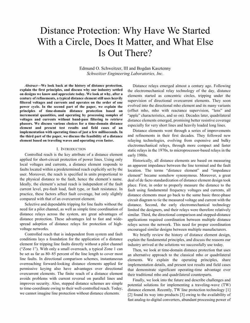
A. Measuring Distance From Voltage and Current Consider the single-phase circuit shown in Fig. 1a. A

distance relay measures the voltage (V) and current (I) at one end of the line. We want a distance element to respond to faults short of a predetermined reach point and restrain for faults beyond that reach point.

(b)Im(Z)

Re(Z)

ZR

•

Reach Point

Z

ZR(a)

I

V

Directional Supervision

(c) Spring

Pivot

RN2 VI N1

Trip Contact

Fig. 1. Distance element reach (a), nondirectional mho characteristic (b), and implementation with a balance beam relay (c).

Let us denote the impedance between the relay and the intended reach point as ZR. We can use the concept of an apparent impedance and complex-number math to define the trip equation of such a distance element:

�𝑉𝑉𝐼𝐼� < |𝑍𝑍𝑅𝑅| (1)

Equation (1) defines a concentric circle on the impedance plane. This operating characteristic is sometimes referred to as an ohm characteristic. Supervising this characteristic with a directional element gives us a forward-looking distance element having a predetermined reach ZR as desired (Fig. 2b).

How can we implement the operating equation (1) in the electromechanical relay technology? We can rewrite (1) in this form:

|𝐼𝐼| >|𝑉𝑉||𝑍𝑍𝑅𝑅| (2)

and observe that (2) compares the magnitude of the relay current (I) with the magnitude of the other current that depends on the relay voltage, V/ZR. We can use the balance-beam electromechanical relay shown in Fig. 1c as the amplitude comparator in (2). The beam pivots toward the coil with the relay current (I) when operating ampere-turns are higher than the restraining ampere-turns:

𝑁𝑁1 ∙ |𝐼𝐼| >|𝑉𝑉|𝑅𝑅∙ 𝑁𝑁2 (3)

or

|𝐼𝐼| >|𝑉𝑉|𝑅𝑅∙𝑁𝑁2𝑁𝑁1

(4)

Comparing (4) with (2), we now have a way to set the relay. We can adjust up to three relay design parameters to obtain the desired reach:

|𝑍𝑍𝑅𝑅| = 𝑅𝑅 ∙𝑁𝑁1𝑁𝑁2

(5)

Equation (5) shows that the element’s reach is controlled by the number of turns of the operating and restraining coils and the resistor used to convert the voltage signal into the current signal. By manipulating these parameters via taps, knobs, and dials, we set such a distance relay.

The distance characteristic in Fig. 1b requires two electromechanical elements: one for measuring the distance and the other for directional supervision. The cost, size, failure modes, and maintenance effort are all proportional to the number of electromechanical elements in a scheme. Can we design a distance scheme that is directional on its own and thus consists of only a single electromechanical element?

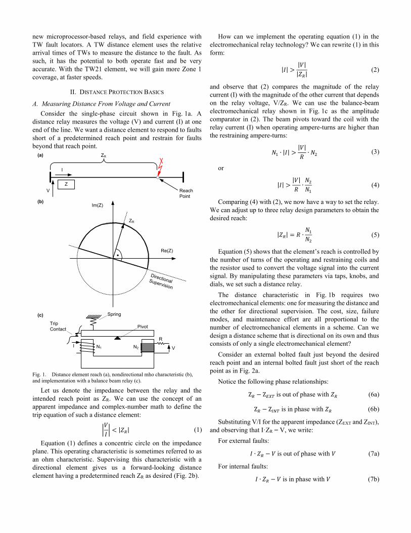
Consider an external bolted fault just beyond the desired reach point and an internal bolted fault just short of the reach point as in Fig. 2a.

Notice the following phase relationships:

Z𝑅𝑅 − Z𝐸𝐸𝐸𝐸𝐸𝐸 is out of phase with 𝑍𝑍𝑅𝑅 (6a)

Z𝑅𝑅 − Z𝐼𝐼𝐼𝐼𝐸𝐸 is in phase with 𝑍𝑍𝑅𝑅 (6b)

Substituting V/I for the apparent impedance (ZEXT and ZINT), and observing that I·ZR = V, we write:

For external faults:

𝐼𝐼 ∙ 𝑍𝑍𝑅𝑅 − 𝑉𝑉 is out of phase with 𝑉𝑉 (7a)

For internal faults:

𝐼𝐼 ∙ 𝑍𝑍𝑅𝑅 − 𝑉𝑉 is in phase with 𝑉𝑉 (7b)

We can draw the threshold in the middle between the “in-phase” (0°) and the “out-of-phase” (180°) values, i.e., at 90°, and write the following trip equation for our distance element:

∠(𝐼𝐼 ∙ 𝑍𝑍𝑅𝑅 − 𝑉𝑉,𝑉𝑉) < ±90° (8)

(a) Im(Z)

Re(Z)

ZEXT

ZR

ZINT

ZR – ZEXT

ZR – ZINT

(b) Im(Z)

Re(Z)

ZR

•

(c)

IPOL

IPOL

IOP

IOP

Trip Contact

Fig. 2. Apparent impedance for external and internal bolted faults (a), directional mho characteristic (b), and a cylinder unit relay (c).

Equation (8) defines a circle that stretches between the origin and the reach point impedance (ZR) on the impedance plane (see Fig. 2b). This operating characteristic is directional on its own, so we do not need the extra directional element to supervise it.

Again, how can we implement the operating equation (8) in the electromechanical relay technology? Equation (8) suggests a phase comparator that can be implemented with a cylinder unit relay (see Fig. 2c). In such a relay, an operating torque is proportional to the sine of the angle between the operating and polarizing currents:

|𝐼𝐼𝑂𝑂𝑂𝑂| ∙ |𝐼𝐼𝑂𝑂𝑂𝑂𝑃𝑃| ∙ sin�∠(𝐼𝐼𝑂𝑂𝑂𝑂, 𝐼𝐼𝑂𝑂𝑂𝑂𝑃𝑃)� (9)

The cylinder unit relay operates when the torque is positive and higher than a small intentional restraint typically provided by a reset spring. We need to connect the cylinder unit relay to proper operating and polarizing currents in order to obtain a cosine comparator for these operating and polarizing signals:

𝑆𝑆𝑂𝑂𝑂𝑂 = 𝐼𝐼 ∙ 𝑍𝑍𝑅𝑅 − 𝑉𝑉 (10)

𝑆𝑆𝑂𝑂𝑂𝑂𝑃𝑃 = 𝑉𝑉 (11)

In the electromechanical relay technology, the operating and restraining signals are created using a mixing circuit with the relay secondary currents and voltages, impedances that replicate the line impedance, and transformers to effectively add signals.

The term I·ZR in the operating signal is a voltage drop from the relay current (I) across the impedance between the relay and the intended reach point (ZR). In the electromechanical relay technology, this voltage is obtained by passing the relay secondary current through an impedance that replicates the line impedance. Accordingly, the term I·ZR is referred to as a replica current, even though the signal is really a voltage. The cylinder unit relay, configured to provide mho distance protection, develops the maximum operating torque when the apparent impedance has the same angle as the reach impedance (ZR). Hence, the angle of ZR defines the maximum torque angle of the mho element.

Another key to a distance element design is to ensure a consistent reach of the element for all fault types on a three-phase line. For phasors only, we can use the positive-sequence voltage and current to measure the distance to the fault. A more advanced solution, common today, is to use six protection loops and select which loop or loops shall be operational for any given fault type. We denote these loops as AG, BG, CG, AB, BC, and CA, each adequate for the corresponding fault type. For each loop, we want to use a loop voltage (VLOOP) and a loop current (ILOOP) such that the apparent impedance between that loop voltage and current is the positive-sequence line impedance between the relay and a zero-resistance (bolted) fault in that loop.

Consider a bolted AG fault. The A-phase voltage at the relay is a voltage drop from the relay current across the impedance between the relay and the fault. We write this voltage as a sum of the sequence voltages:

𝑉𝑉𝐴𝐴 = 𝑉𝑉1 + 𝑉𝑉2 + 𝑉𝑉0 (12)

Assuming Z2 = Z1 for the line, we rewrite (12) as follows:

𝑉𝑉𝐴𝐴 = 𝑍𝑍1(𝐼𝐼1 + 𝐼𝐼2) + 𝑍𝑍0𝐼𝐼0 (13)

Because 𝐼𝐼1 + 𝐼𝐼2 = 𝐼𝐼𝐴𝐴 − 𝐼𝐼0 we write:

𝑉𝑉𝐴𝐴 = 𝑍𝑍1𝐼𝐼𝐴𝐴 + 𝑍𝑍0𝐼𝐼0 − 𝑍𝑍1𝐼𝐼0 (14)

Further:

𝑉𝑉𝐴𝐴 = 𝑍𝑍1 �𝐼𝐼𝐴𝐴 +𝑍𝑍0 − 𝑍𝑍1𝑍𝑍1

𝐼𝐼0� = 𝑍𝑍1 �𝐼𝐼𝐴𝐴 +𝑍𝑍0 − 𝑍𝑍1

3𝑍𝑍1𝐼𝐼𝐺𝐺� (15)

From (15) we see that if we use:

𝑉𝑉𝑃𝑃𝐿𝐿𝐿𝐿𝐿𝐿 = 𝑉𝑉𝐴𝐴 and 𝐼𝐼𝑃𝑃𝐿𝐿𝐿𝐿𝐿𝐿 = 𝐼𝐼𝐴𝐴 +𝑍𝑍0 − 𝑍𝑍1

3𝑍𝑍1𝐼𝐼𝐺𝐺 (16)

we will measure the positive-sequence impedance between the relay and a bolted AG fault. We derive similar loop voltages and currents for the other five protection loops.

In a six-loop (six-element) distance scheme, the replica currents are derived in the mixing circuit for each of the six protection loops using both the zero- and positive-sequence line impedances.

Ideally, each loop works with a separate measuring relay. In order to avoid having six measuring relays, electromechanical designs often used a switched distance scheme. In a switched scheme, a single measuring relay was switched onto the right

pair of polarizing and operating signals based on the fault type, upon the assertion of a starting unit. Similarly, multiple zones of stepped distance protection were achieved by switching the reach of a single measuring unit to transition from one zone to the next after the previous zone timer expired and no trip was asserted. Switched distance schemes are not used anymore, because they are slower and internally more complicated than the six-loop multizone schemes.

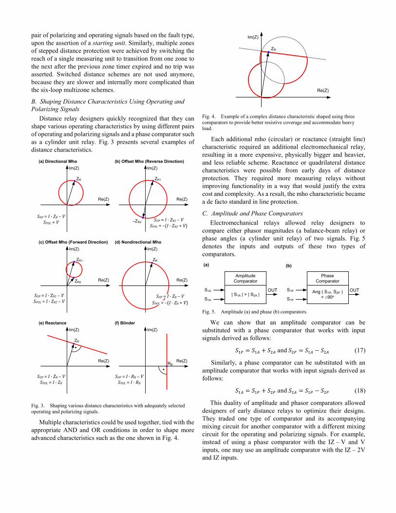
B. Shaping Distance Characteristics Using Operating and Polarizing Signals

Distance relay designers quickly recognized that they can shape various operating characteristics by using different pairs of operating and polarizing signals and a phase comparator such as a cylinder unit relay. Fig. 3 presents several examples of distance characteristics.

(a) Directional Mho (b) Offset Mho (Reverse Direction)Im(Z)

Re(Z)

ZR

Im(Z)

Re(Z)

ZR1

–ZR2

Im(Z)

Re(Z)

ZR1

ZR2

Im(Z)

Re(Z)

ZR

(c) Offset Mho (Forward Direction) (d) Nondirectional Mho

Im(Z)

Re(Z)

ZR

Im(Z)

Re(Z)RB

(e) Reactance (f) Blinder

SOP = I · ZR – VSPOL = V SOP = I · ZR1 – V

SPOL = –(I · ZR2 + V)

SOP = I · ZR1 – VSPOL = I · ZR2 – V

SOP = I · ZR – VSPOL = I · ZR

SOP = I · RB – VSPOL = I · RB

SPOL = –(I · ZR + V)SOP = I · ZR – V

Fig. 3. Shaping various distance characteristics with adequately selected operating and polarizing signals.

Multiple characteristics could be used together, tied with the appropriate AND and OR conditions in order to shape more advanced characteristics such as the one shown in Fig. 4.

Im(Z)

Re(Z)

ZR

Fig. 4. Example of a complex distance characteristic shaped using three comparators to provide better resistive coverage and accommodate heavy load.

Each additional mho (circular) or reactance (straight line) characteristic required an additional electromechanical relay, resulting in a more expensive, physically bigger and heavier, and less reliable scheme. Reactance or quadrilateral distance characteristics were possible from early days of distance protection. They required more measuring relays without improving functionality in a way that would justify the extra cost and complexity. As a result, the mho characteristic became a de facto standard in line protection.

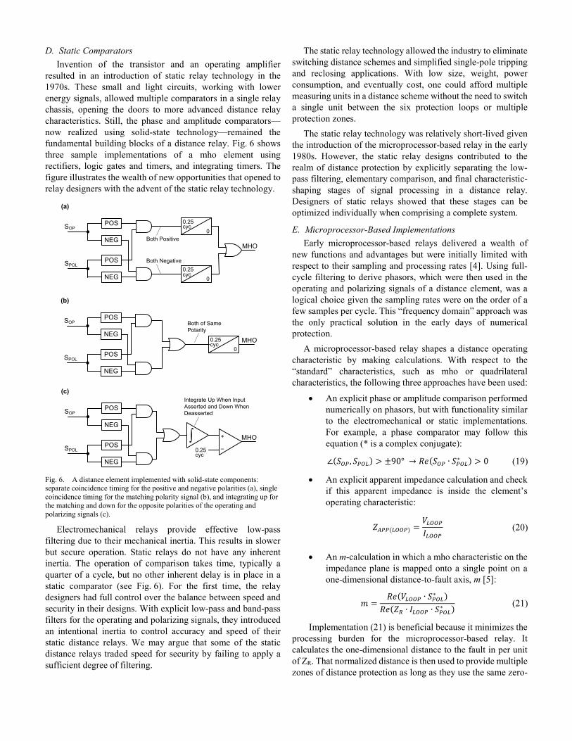
C. Amplitude and Phase Comparators Electromechanical relays allowed relay designers to

compare either phasor magnitudes (a balance-beam relay) or phase angles (a cylinder unit relay) of two signals. Fig. 5 denotes the inputs and outputs of these two types of comparators.

AmplitudeComparator

| S1A | > | S2A |S1A

S1A

(a)

Phase Comparator

Ang ( S1P, S2P ) > ±90o

OUT

(b)

S1P

S1P

OUT

Fig. 5. Amplitude (a) and phase (b) comparators.

We can show that an amplitude comparator can be substituted with a phase comparator that works with input signals derived as follows:

𝑆𝑆1𝑂𝑂 = 𝑆𝑆1𝐴𝐴 + 𝑆𝑆2𝐴𝐴 and 𝑆𝑆2𝑂𝑂 = 𝑆𝑆1𝐴𝐴 − 𝑆𝑆2𝐴𝐴 (17)

Similarly, a phase comparator can be substituted with an amplitude comparator that works with input signals derived as follows:

𝑆𝑆1𝐴𝐴 = 𝑆𝑆1𝑂𝑂 + 𝑆𝑆2𝑂𝑂 and 𝑆𝑆2𝐴𝐴 = 𝑆𝑆1𝑂𝑂 − 𝑆𝑆2𝑂𝑂 (18)

This duality of amplitude and phasor comparators allowed designers of early distance relays to optimize their designs. They traded one type of comparator and its accompanying mixing circuit for another comparator with a different mixing circuit for the operating and polarizing signals. For example, instead of using a phase comparator with the IZ – V and V inputs, one may use an amplitude comparator with the IZ – 2V and IZ inputs.

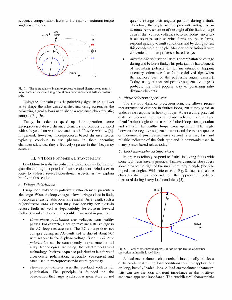
D. Static Comparators Invention of the transistor and an operating amplifier

resulted in an introduction of static relay technology in the 1970s. These small and light circuits, working with lower energy signals, allowed multiple comparators in a single relay chassis, opening the doors to more advanced distance relay characteristics. Still, the phase and amplitude comparators—now realized using solid-state technology—remained the fundamental building blocks of a distance relay. Fig. 6 shows three sample implementations of a mho element using rectifiers, logic gates and timers, and integrating timers. The figure illustrates the wealth of new opportunities that opened to relay designers with the advent of the static relay technology.

SOP

Both Positive

POS

NEG

cyc0.25

0

SPOLPOS

NEG

Both Negative

MHO

(a)

SOP Both of Same Polarity

POS

NEGcyc0.25

0SPOL

POS

NEG

MHO

(b)

SOP

Integrate Up When Input Asserted and Down When Deasserted

POS

NEG

cyc0.25SPOL

POS

NEG

MHO

(c)

∫ +

–

cyc0.25

0

Fig. 6. A distance element implemented with solid-state components: separate coincidence timing for the positive and negative polarities (a), single coincidence timing for the matching polarity signal (b), and integrating up for the matching and down for the opposite polarities of the operating and polarizing signals (c).

Electromechanical relays provide effective low-pass filtering due to their mechanical inertia. This results in slower but secure operation. Static relays do not have any inherent inertia. The operation of comparison takes time, typically a quarter of a cycle, but no other inherent delay is in place in a static comparator (see Fig. 6). For the first time, the relay designers had full control over the balance between speed and security in their designs. With explicit low-pass and band-pass filters for the operating and polarizing signals, they introduced an intentional inertia to control accuracy and speed of their static distance relays. We may argue that some of the static distance relays traded speed for security by failing to apply a sufficient degree of filtering.

The static relay technology allowed the industry to eliminate switching distance schemes and simplified single-pole tripping and reclosing applications. With low size, weight, power consumption, and eventually cost, one could afford multiple measuring units in a distance scheme without the need to switch a single unit between the six protection loops or multiple protection zones.

The static relay technology was relatively short-lived given the introduction of the microprocessor-based relay in the early 1980s. However, the static relay designs contributed to the realm of distance protection by explicitly separating the low-pass filtering, elementary comparison, and final characteristic-shaping stages of signal processing in a distance relay. Designers of static relays showed that these stages can be optimized individually when comprising a complete system.

E. Microprocessor-Based Implementations Early microprocessor-based relays delivered a wealth of

new functions and advantages but were initially limited with respect to their sampling and processing rates [4]. Using full-cycle filtering to derive phasors, which were then used in the operating and polarizing signals of a distance element, was a logical choice given the sampling rates were on the order of a few samples per cycle. This “frequency domain” approach was the only practical solution in the early days of numerical protection.

A microprocessor-based relay shapes a distance operating characteristic by making calculations. With respect to the “standard” characteristics, such as mho or quadrilateral characteristics, the following three approaches have been used:

• An explicit phase or amplitude comparison performed numerically on phasors, but with functionality similar to the electromechanical or static implementations. For example, a phase comparator may follow this equation (* is a complex conjugate):

∠(𝑆𝑆𝑂𝑂𝑂𝑂 , 𝑆𝑆𝑂𝑂𝑂𝑂𝑃𝑃) > ±90° → 𝑅𝑅𝑅𝑅(𝑆𝑆𝑂𝑂𝑂𝑂 ∙ 𝑆𝑆𝑂𝑂𝑂𝑂𝑃𝑃∗ ) > 0 (19)

• An explicit apparent impedance calculation and check if this apparent impedance is inside the element’s operating characteristic:

𝑍𝑍𝐴𝐴𝑂𝑂𝑂𝑂(𝑃𝑃𝑂𝑂𝑂𝑂𝑂𝑂) =𝑉𝑉𝑃𝑃𝑂𝑂𝑂𝑂𝑂𝑂𝐼𝐼𝑃𝑃𝑂𝑂𝑂𝑂𝑂𝑂

(20)

• An m-calculation in which a mho characteristic on the impedance plane is mapped onto a single point on a one-dimensional distance-to-fault axis, m [5]:

𝑚𝑚 =𝑅𝑅𝑅𝑅(𝑉𝑉𝑃𝑃𝑂𝑂𝑂𝑂𝑂𝑂 ∙ 𝑆𝑆𝑂𝑂𝑂𝑂𝑃𝑃∗ )

𝑅𝑅𝑅𝑅(𝑍𝑍𝑅𝑅 ∙ 𝐼𝐼𝑃𝑃𝑂𝑂𝑂𝑂𝑂𝑂 ∙ 𝑆𝑆𝑂𝑂𝑂𝑂𝑃𝑃∗ ) (21)

Implementation (21) is beneficial because it minimizes the processing burden for the microprocessor-based relay. It calculates the one-dimensional distance to the fault in per unit of ZR. That normalized distance is then used to provide multiple zones of distance protection as long as they use the same zero-

sequence compensation factor and the same maximum torque angle (see Fig. 7).

Im(Z)

Re(Z)

ZR

Line Angle m

0

1

Fig. 7. The m-calculation in a microprocessor-based distance relay maps a mho characteristic onto a single point on a one-dimensional distance-to-fault axis.

Using the loop voltage as the polarizing signal in (21) allows us to shape the mho characteristic, and using current as the polarizing signal allows us to shape a reactance characteristic; compare Fig. 3e.

Today, in order to speed up their operation, some microprocessor-based distance elements use phasors obtained with subcycle data windows, such as a half-cycle window [6]. In general, however, microprocessor-based distance relays typically continue to use phasors in their operating characteristics, i.e., they effectively operate in the “frequency domain.”

III. V/I DOES NOT MAKE A DISTANCE RELAY In addition to a distance-shaping logic, such as the mho or

quadrilateral logic, a practical distance element includes extra logic to address several operational aspects, as we explain briefly in this section.

A. Voltage Polarization Using loop voltage to polarize a mho element presents a

challenge. When the loop voltage is low during a close-in fault, it becomes a less reliable polarizing signal. As a result, such a self-polarized mho element may lose security for close-in reverse faults as well as dependability for close-in forward faults. Several solutions to this problem are used in practice:

• Cross-phase polarization uses voltages from healthy phases. For example, a design may use a BC voltage in the AG loop measurement. The BC voltage does not collapse during an AG fault and is shifted about 90° with respect to the A-phase voltage. Such quadrature polarization can be conveniently implemented in all relay technologies including the electromechanical technology. Positive-sequence polarization is a form of cross-phase polarization, especially convenient and often used in microprocessor-based relays today.

• Memory polarization uses the pre-fault voltage for polarization. The principle is founded on the observation that large synchronous generators do not

quickly change their angular position during a fault. Therefore, the angle of the pre-fault voltage is an accurate representation of the angle of the fault voltage even if that voltage collapses to zero. Today, inverter-based sources, such as wind farms and solar farms, respond quickly to fault conditions and by doing so test this decades-old principle. Memory polarization is very convenient in microprocessor-based relays.

• Mixed-mode polarization uses a combination of voltage during and before a fault. This polarization has a benefit of providing polarization for instantaneous tripping (memory action) as well as for time-delayed trips (when the memory part of the polarizing signal expires). Today, using memorized positive-sequence voltage is probably the most popular way of polarizing mho distance elements.

B. Phase Selection Supervision The six-loop distance protection principle allows proper

measurement of distance in faulted loops, but it may yield an undesirable response in healthy loops. As a result, a practical distance element requires a phase selection (fault type identification) logic to release the faulted loops for operation and restrain the healthy loops from operation. The angle between the negative-sequence current and the zero-sequence or incremental positive-sequence current is a very fast and reliable indicator of the fault type and is commonly used in many phasor-based relays today.

C. Load-Encroachment Supervision In order to reliably respond to faults, including faults with

some fault resistance, a practical distance characteristic covers some area to the right of the maximum torque angle (the line impedance angle). With reference to Fig. 8, such a distance characteristic may encroach on the apparent impedance measured during heavy load conditions [5].

Im(Z)

Re(Z)

ZR

Fig. 8. Load-encroachment supervision for the application of distance protection on heavily loaded lines.

A load-encroachment characteristic intentionally blocks a distance element during load conditions to allow applications on long, heavily loaded lines. A load-encroachment character-istic can use the loop apparent impedance or the positive-sequence apparent impedance. The quadrilateral characteristic

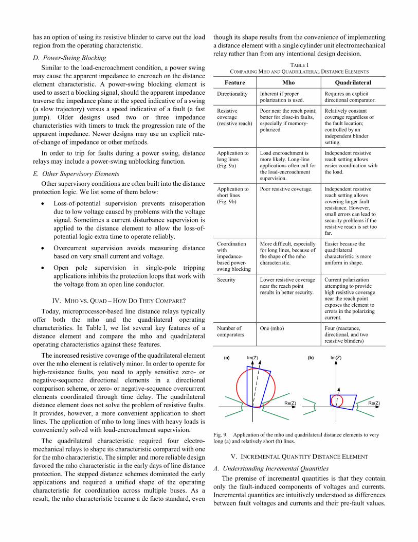
has an option of using its resistive blinder to carve out the load region from the operating characteristic.

D. Power-Swing Blocking Similar to the load-encroachment condition, a power swing

may cause the apparent impedance to encroach on the distance element characteristic. A power-swing blocking element is used to assert a blocking signal, should the apparent impedance traverse the impedance plane at the speed indicative of a swing (a slow trajectory) versus a speed indicative of a fault (a fast jump). Older designs used two or three impedance characteristics with timers to track the progression rate of the apparent impedance. Newer designs may use an explicit rate-of-change of impedance or other methods.

In order to trip for faults during a power swing, distance relays may include a power-swing unblocking function.

E. Other Supervisory Elements Other supervisory conditions are often built into the distance

protection logic. We list some of them below:

• Loss-of-potential supervision prevents misoperation due to low voltage caused by problems with the voltage signal. Sometimes a current disturbance supervision is applied to the distance element to allow the loss-of-potential logic extra time to operate reliably.

• Overcurrent supervision avoids measuring distance based on very small current and voltage.

• Open pole supervision in single-pole tripping applications inhibits the protection loops that work with the voltage from an open line conductor.

IV. MHO VS. QUAD – HOW DO THEY COMPARE? Today, microprocessor-based line distance relays typically

offer both the mho and the quadrilateral operating characteristics. In Table I, we list several key features of a distance element and compare the mho and quadrilateral operating characteristics against these features.

The increased resistive coverage of the quadrilateral element over the mho element is relatively minor. In order to operate for high-resistance faults, you need to apply sensitive zero- or negative-sequence directional elements in a directional comparison scheme, or zero- or negative-sequence overcurrent elements coordinated through time delay. The quadrilateral distance element does not solve the problem of resistive faults. It provides, however, a more convenient application to short lines. The application of mho to long lines with heavy loads is conveniently solved with load-encroachment supervision.

The quadrilateral characteristic required four electro-mechanical relays to shape its characteristic compared with one for the mho characteristic. The simpler and more reliable design favored the mho characteristic in the early days of line distance protection. The stepped distance schemes dominated the early applications and required a unified shape of the operating characteristic for coordination across multiple buses. As a result, the mho characteristic became a de facto standard, even

though its shape results from the convenience of implementing a distance element with a single cylinder unit electromechanical relay rather than from any intentional design decision.

TABLE I COMPARING MHO AND QUADRILATERAL DISTANCE ELEMENTS

Feature Mho Quadrilateral

Directionality Inherent if proper polarization is used.

Requires an explicit directional comparator.

Resistive coverage (resistive reach)

Poor near the reach point; better for close-in faults, especially if memory-polarized.

Relatively constant coverage regardless of the fault location; controlled by an independent blinder setting.

Application to long lines (Fig. 9a)

Load encroachment is more likely. Long-line applications often call for the load-encroachment supervision.

Independent resistive reach setting allows easier coordination with the load.

Application to short lines (Fig. 9b)

Poor resistive coverage. Independent resistive reach setting allows covering larger fault resistance. However, small errors can lead to security problems if the resistive reach is set too far.

Coordination with impedance- based power-swing blocking

More difficult, especially for long lines, because of the shape of the mho characteristic.

Easier because the quadrilateral characteristic is more uniform in shape.

Security Lower resistive coverage near the reach point results in better security.

Current polarization attempting to provide high resistive coverage near the reach point exposes the element to errors in the polarizing current.

Number of comparators

One (mho) Four (reactance, directional, and two resistive blinders)

Im(Z)

Re(Z)

(a) Im(Z)

Re(Z)

(b)

Fig. 9. Application of the mho and quadrilateral distance elements to very long (a) and relatively short (b) lines.

V. INCREMENTAL QUANTITY DISTANCE ELEMENT

A. Understanding Incremental Quantities The premise of incremental quantities is that they contain

only the fault-induced components of voltages and currents. Incremental quantities are intuitively understood as differences between fault voltages and currents and their pre-fault values.

“Incremental quantity” is, however, a relatively broad term. We can explain the many types of incremental quantities by referring to a range of filtering options practically used in power system protection to obtain these quantities:

• An instantaneous incremental quantity is obtained by subtracting the present (fault) value and the memorized pre-fault value (typically, several cycles old) in time domain. As such, this incremental quantity contains all frequency components present in the fault signal, including the decaying dc offset, the fault component of the fundamental frequency signal, and the high-frequency transients. This type of incremental quantity contains the maximum possible amount of information. Because it is calculated using a memorized value, this type of incremental quantity becomes invalid as soon as the memory expires. In our implementation [3], we use this type of incremental quantity with a one-cycle memory buffer.

• A phasor incremental quantity is obtained by subtracting the present (fault) value and the pre-fault value (typically, several cycles old) in frequency domain. As such, this incremental quantity is a phasor that is band-pass filtered to intentionally retain only the fundamental frequency information present in the fault quantity at the expense of filtering latency and slower operation. Using memory, this kind of incremental quantity also expires with time. Some of our protection implementations [7] obtain this type of incremental quantity using a half-cycle Fourier filter with a two-cycle memory buffer. Negative- and zero-sequence quantities are ideally zero in the pre-fault state. As such, they are effectively incremental quantities as well. A phasor incremental quantity can be obtained by extracting a phasor from the instantaneous incremental quantity.

• A high-frequency incremental quantity is obtained by high-pass filtering of the input signal. As such, this incremental quantity contains high-frequency components, excluding the fundamental frequency information present in the fault signal. Using high-pass filtering, this kind of incremental signal is short-lived (a few milliseconds at best), and it reoccurs on every sharp change in the input signal. A high-frequency incremental quantity is relatively easy to obtain using static relay technology and was therefore used in early implementations of ultra-high-speed relays [8] [9] [10]. Depending on the upper limit of the frequency spectrum, we may refer to the signal obtained through high-pass filtering as an “incremental quantity” (the spectrum is in the range of up to a few kilohertz) or a “traveling wave” (the spectrum is in the range of a few hundred kilohertz). Some past implementations of ultra-high-speed relays have been mislabeled as traveling-wave relays.

• A time derivative of a signal is one specific version of high-pass filtering. Solutions that use differentiation, or differentiation combined with smoothing, to extract time-domain features of the signal with microsecond resolution are referred to as traveling-wave techniques [1] [2].

Traveling waves are technically a form of incremental quantities. However, they carry considerable information in their arrival times in addition to information in relative polarities and magnitudes. We describe a TW-based distance element in Section VI.

Instantaneous incremental quantities are often low-pass filtered to limit the frequency band to about 300 Hz to 1 kHz. This allows the relay designers to represent the protected line and the system with an equivalent resistive-inductive (RL) circuit, simplifying the operating equations for the incremental quantity protection elements. Microprocessor-based relays typically execute the instantaneous incremental quantity calculations and logic at the rate of 5 to 10 kHz [3].

In this section, we derive an underreaching distance element based on incremental quantities and show its various implementations depending on the type of incremental quantity used and other practical considerations.

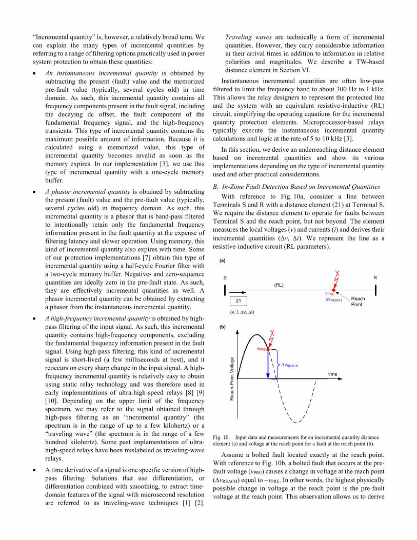
B. In-Zone Fault Detection Based on Incremental Quantities With reference to Fig. 10a, consider a line between

Terminals S and R with a distance element (21) at Terminal S. We require the distance element to operate for faults between Terminal S and the reach point, but not beyond. The element measures the local voltages (v) and currents (i) and derives their incremental quantities (∆v, ∆i). We represent the line as a resistive-inductive circuit (RL parameters).

S R

Reach Point

21

(RL)

Rea

ch-P

oint

Vol

tage

time

vPRE

∆vREACH

(a)

(b)

(v, i, ∆v, ∆i)

vPRE

∆vREACH

Fig. 10. Input data and measurements for an incremental quantity distance element (a) and voltage at the reach point for a fault at the reach point (b).

Assume a bolted fault located exactly at the reach point. With reference to Fig. 10b, a bolted fault that occurs at the pre-fault voltage (vPRE) causes a change in voltage at the reach point (∆vREACH) equal to −vPRE. In other words, the highest physically possible change in voltage at the reach point is the pre-fault voltage at the reach point. This observation allows us to derive

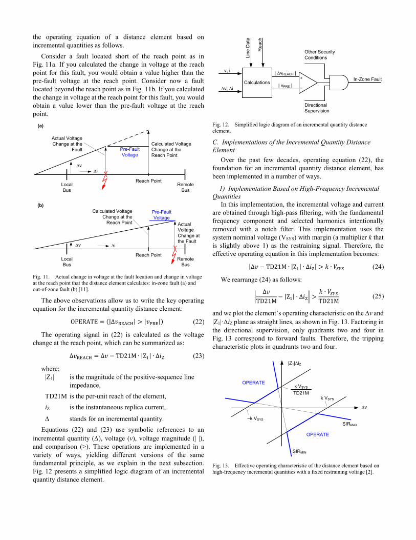
the operating equation of a distance element based on incremental quantities as follows.

Consider a fault located short of the reach point as in Fig. 11a. If you calculated the change in voltage at the reach point for this fault, you would obtain a value higher than the pre-fault voltage at the reach point. Consider now a fault located beyond the reach point as in Fig. 11b. If you calculated the change in voltage at the reach point for this fault, you would obtain a value lower than the pre-fault voltage at the reach point.

(a)

∆v∆i

(b)

Remote Bus

Calculated Voltage Change at the Reach Point

Reach PointLocal Bus

Actual Voltage Change at the

Fault

∆v ∆i

Remote Bus

Local Bus

Calculated Voltage Change at the

Reach Point Actual Voltage Change at the Fault

Reach Point

Pre-Fault Voltage

Pre-Fault Voltage

Fig. 11. Actual change in voltage at the fault location and change in voltage at the reach point that the distance element calculates: in-zone fault (a) and out-of-zone fault (b) [11].

The above observations allow us to write the key operating equation for the incremental quantity distance element:

OPERATE = (|∆𝑣𝑣REACH| > |𝑣𝑣PRE|) (22)

The operating signal in (22) is calculated as the voltage change at the reach point, which can be summarized as:

∆𝑣𝑣REACH = ∆𝑣𝑣 − TD21M ∙ |Z1| ∙ ∆𝑖𝑖Z (23)

where: |Z1| is the magnitude of the positive-sequence line

impedance, TD21M is the per-unit reach of the element, iZ is the instantaneous replica current,

∆ stands for an incremental quantity. Equations (22) and (23) use symbolic references to an

incremental quantity (∆), voltage (v), voltage magnitude (| |), and comparison (>). These operations are implemented in a variety of ways, yielding different versions of the same fundamental principle, as we explain in the next subsection. Fig. 12 presents a simplified logic diagram of an incremental quantity distance element.

_

+Calculations

| ∆vREACH |

Directional Supervision

Other Security Conditions

In-Zone Fault

Rea

ch

| vPRE |

v, i

∆v, ∆i

Line

Dat

a

Fig. 12. Simplified logic diagram of an incremental quantity distance element.

C. Implementations of the Incremental Quantity Distance Element

Over the past few decades, operating equation (22), the foundation for an incremental quantity distance element, has been implemented in a number of ways.

1) Implementation Based on High-Frequency Incremental Quantities

In this implementation, the incremental voltage and current are obtained through high-pass filtering, with the fundamental frequency component and selected harmonics intentionally removed with a notch filter. This implementation uses the system nominal voltage (VSYS) with margin (a multiplier k that is slightly above 1) as the restraining signal. Therefore, the effective operating equation in this implementation becomes:

|∆𝑣𝑣 − TD21M ∙ |Z1| ∙ ∆𝑖𝑖Z| > 𝑘𝑘 ∙ 𝑉𝑉𝑆𝑆𝑆𝑆𝑆𝑆 (24)

We rearrange (24) as follows:

�∆𝑣𝑣

TD21M− |Z1| ∙ ∆𝑖𝑖Z� >

𝑘𝑘 ∙ 𝑉𝑉𝑆𝑆𝑆𝑆𝑆𝑆TD21M

(25)

and we plot the element’s operating characteristic on the ∆v and |Z1|·∆iZ plane as straight lines, as shown in Fig. 13. Factoring in the directional supervision, only quadrants two and four in Fig. 13 correspond to forward faults. Therefore, the tripping characteristic plots in quadrants two and four.

OPERATE

OPERATE

SIRMAX

SIRMIN

|Z1|∆iZ

∆v

k VSYS

TD21M

–k VSYS

k VSYS

Fig. 13. Effective operating characteristic of the distance element based on high-frequency incremental quantities with a fixed restraining voltage [2].

We also remember that for a forward fault, the incremental voltage and incremental replica currents are tied together as follows:

∆𝑣𝑣 = −|ZSYS| ∙ ∆𝑖𝑖Z = −SIR ∙ |Z1| ∙ ∆𝑖𝑖Z (26)

where: |ZSYS| is the magnitude of the positive-sequence

impedance of the system behind the relay, SIR is the source-to-line impedance ratio.

Equation (26) further limits the operating region in Fig. 13, assuming the minimum and maximum SIR values of any given application.

This type of an incremental quantity distance element was originally introduced by Chamia and Liberman [8]; Engler, Lanz, Hanggli, and Bacchini [9]; and Vitins [10]. These imple-mentations were known to trip for heavy, close-in faults in less than half a power cycle.

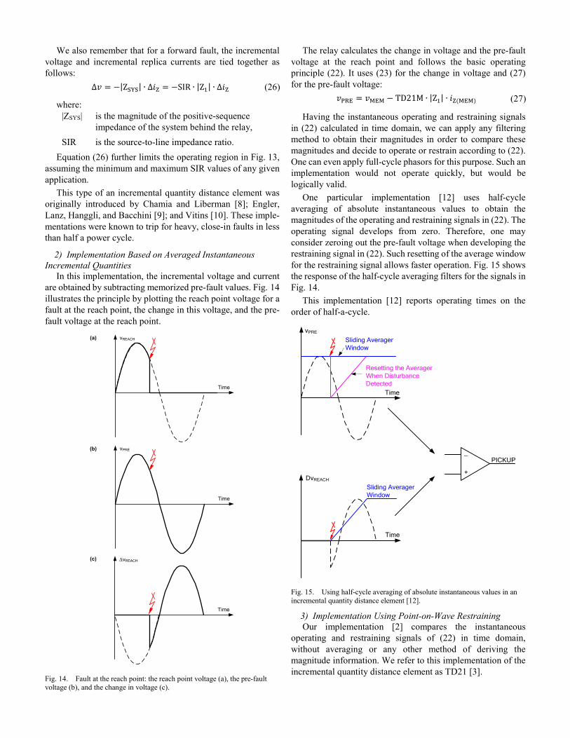
2) Implementation Based on Averaged Instantaneous Incremental Quantities

In this implementation, the incremental voltage and current are obtained by subtracting memorized pre-fault values. Fig. 14 illustrates the principle by plotting the reach point voltage for a fault at the reach point, the change in this voltage, and the pre-fault voltage at the reach point.

Time

vREACH

Time

vPRE

Time

∆vREACH

(a)

(b)

(c)

Fig. 14. Fault at the reach point: the reach point voltage (a), the pre-fault voltage (b), and the change in voltage (c).

The relay calculates the change in voltage and the pre-fault voltage at the reach point and follows the basic operating principle (22). It uses (23) for the change in voltage and (27) for the pre-fault voltage:

𝑣𝑣PRE = 𝑣𝑣MEM − TD21M ∙ |Z1| ∙ 𝑖𝑖Z(MEM) (27)

Having the instantaneous operating and restraining signals in (22) calculated in time domain, we can apply any filtering method to obtain their magnitudes in order to compare these magnitudes and decide to operate or restrain according to (22). One can even apply full-cycle phasors for this purpose. Such an implementation would not operate quickly, but would be logically valid.

One particular implementation [12] uses half-cycle averaging of absolute instantaneous values to obtain the magnitudes of the operating and restraining signals in (22). The operating signal develops from zero. Therefore, one may consider zeroing out the pre-fault voltage when developing the restraining signal in (22). Such resetting of the average window for the restraining signal allows faster operation. Fig. 15 shows the response of the half-cycle averaging filters for the signals in Fig. 14.

This implementation [12] reports operating times on the order of half-a-cycle.

Time

vPRE

Time

DvREACH

Resetting the Averager When Disturbance Detected

Sliding Averager Window

Sliding Averager Window

_

+

PICKUP

Fig. 15. Using half-cycle averaging of absolute instantaneous values in an incremental quantity distance element [12].

3) Implementation Using Point-on-Wave Restraining Our implementation [2] compares the instantaneous

operating and restraining signals of (22) in time domain, without averaging or any other method of deriving the magnitude information. We refer to this implementation of the incremental quantity distance element as TD21 [3].

To use the concept of point-on-wave restraining, we calculate the instantaneous voltage at the reach point. We know that the restraining voltage calculated with (27) is not perfectly accurate because of the finite precision of line impedance data, charging current, line transposition, and so on [2]. Nonetheless, (27) is a good approximation of the actual voltage at the reach point. Of course, we need the delayed value of (27) to represent the voltage at the reach point prior to the fault.

Fig. 16 explains our implementation. We multiply the absolute value of the voltage (27) by the factor k (slightly above 1) to add a small amplitude margin and buffer it. We extract one-period-old data and two extra sets of data—one ahead and one beyond the exact one-period-old data—to add a small phase margin. The maximum value among the minimum restraint level and the three values becomes the final restraint, V21RST. We use the minimum restraint constant to ensure that the TD21 restraint does not fall to zero for points on wave near the zero crossings (i.e., during time intervals when the restraining signal (27) is very small or zero).

Fig. 16b illustrates the rationale of the way we calculate the TD21 restraining voltage. Our goal is to create a signal that envelops the actual reach point voltage while assuming various sources of errors, yet is as small as possible to maintain the speed and sensitivity inherent in the time-domain implementation. We refer to the restraint of Fig. 16b as a point-on-wave restraint to contrast it with the two competing solutions: the constant, worst-case restraint equals the nominal system voltage plus margin (24) and the half-cycle averaged value (Fig. 15).

k BUFFER

MAX

1 period

Minimum Restraining

Level

abs

(a)

Time

Minimum Restraining Level

Final Restraining Signal

Actual Reach-Point Voltage

Security Bands

Calculated Reach-Point

Voltage

Calculated Instantaneous Reach-Point Voltage

(b)

V21RST

Volta

ge

Fig. 16. Calculations of the point-on-wave TD21 restraining signal: logic diagram (a) and example of operation (b) [13].

After calculating the operating and restraining signals, we compare them as shown in Fig. 17. We determine if the operating signal is above the restraining signal by integrating the difference between the two signals. We run the integrator if

the loop is involved in the fault and if the incremental voltage at the reach point is attributed to a voltage decrease (collapse). In general, the incremental voltage at the reach point may result from any voltage change, either a voltage decrease or increase.

Σ+

¯

∆vREACH

V21RST

∫ +

¯Overcurrent Supervision

TD21PKPRUN

Loop Involved in Fault

Reach-Point Voltage Collapse

| ∆vREACH | > V21RST

Security Margin

E21

abs

Fig. 17. TD21 integration and comparison logic [13].

We allow the TD21 to integrate only if the voltage has collapsed. We confirm the collapse by checking the relative polarity between the restraining voltage, vPRE in (27), prior to the fault and the operating voltage, ∆vREACH in (23). For a fault, the incremental voltage at the fault should be negative for a positive restraining voltage and vice versa (see Fig. 14 for an illustration). The voltage collapse check provides extra security against switching events. By applying this check, the TD21 element effectively responds to a signed restraining voltage, not the absolute value of it.

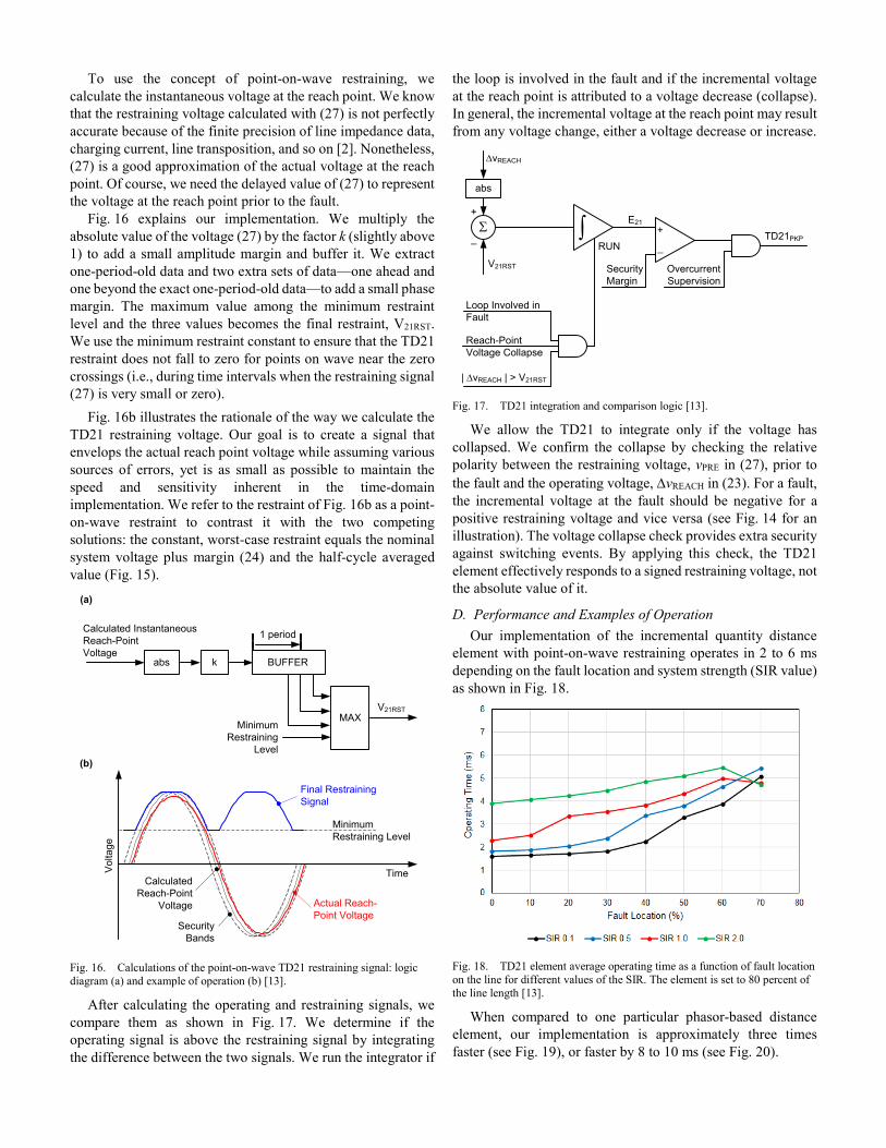
D. Performance and Examples of Operation Our implementation of the incremental quantity distance

element with point-on-wave restraining operates in 2 to 6 ms depending on the fault location and system strength (SIR value) as shown in Fig. 18.

Fig. 18. TD21 element average operating time as a function of fault location on the line for different values of the SIR. The element is set to 80 percent of the line length [13].

When compared to one particular phasor-based distance element, our implementation is approximately three times faster (see Fig. 19), or faster by 8 to 10 ms (see Fig. 20).

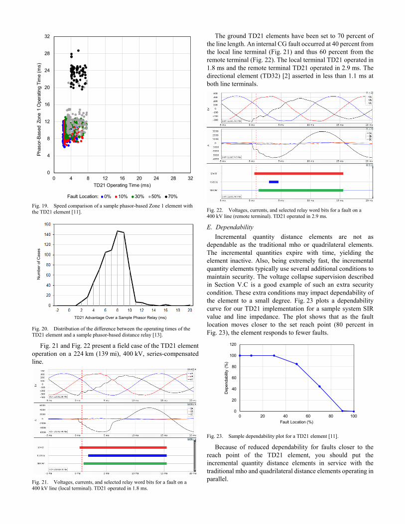
Fig. 19. Speed comparison of a sample phasor-based Zone 1 element with the TD21 element [11].

Num

ber o

f Cas

es

TD21 Advantage Over a Sample Phasor Relay (ms)

Fig. 20. Distribution of the difference between the operating times of the TD21 element and a sample phasor-based distance relay [13].

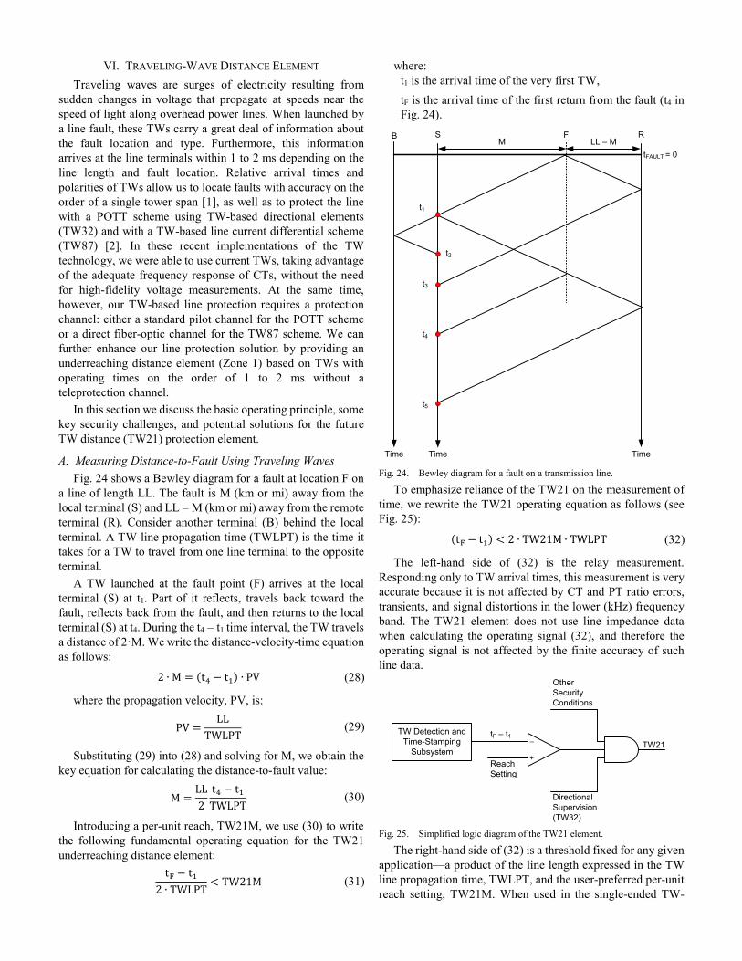
Fig. 21 and Fig. 22 present a field case of the TD21 element operation on a 224 km (139 mi), 400 kV, series-compensated line.

Fig. 21. Voltages, currents, and selected relay word bits for a fault on a 400 kV line (local terminal). TD21 operated in 1.8 ms.

The ground TD21 elements have been set to 70 percent of the line length. An internal CG fault occurred at 40 percent from the local line terminal (Fig. 21) and thus 60 percent from the remote terminal (Fig. 22). The local terminal TD21 operated in 1.8 ms and the remote terminal TD21 operated in 2.9 ms. The directional element (TD32) [2] asserted in less than 1.1 ms at both line terminals.

Fig. 22. Voltages, currents, and selected relay word bits for a fault on a 400 kV line (remote terminal). TD21 operated in 2.9 ms.

E. Dependability Incremental quantity distance elements are not as

dependable as the traditional mho or quadrilateral elements. The incremental quantities expire with time, yielding the element inactive. Also, being extremely fast, the incremental quantity elements typically use several additional conditions to maintain security. The voltage collapse supervision described in Section V.C is a good example of such an extra security condition. These extra conditions may impact dependability of the element to a small degree. Fig. 23 plots a dependability curve for our TD21 implementation for a sample system SIR value and line impedance. The plot shows that as the fault location moves closer to the set reach point (80 percent in Fig. 23), the element responds to fewer faults.

Fig. 23. Sample dependability plot for a TD21 element [11].

Because of reduced dependability for faults closer to the reach point of the TD21 element, you should put the incremental quantity distance elements in service with the traditional mho and quadrilateral distance elements operating in parallel.

0

4

8

12

16

20

24

28

32

0 4 8 12 16 20 24 28 32

Phas

or-B

ased

Zon

e 1

Ope

ratin

g Ti

me

(ms)

TD21 Operating Time (ms)

0% 10% 30% 50% 70%Fault Location:

0

20

40

60

80

100

120

0 20 40 60 80 100

Dep

enda

bility

(%

)

Fault Location (%)

VI. TRAVELING-WAVE DISTANCE ELEMENT Traveling waves are surges of electricity resulting from

sudden changes in voltage that propagate at speeds near the speed of light along overhead power lines. When launched by a line fault, these TWs carry a great deal of information about the fault location and type. Furthermore, this information arrives at the line terminals within 1 to 2 ms depending on the line length and fault location. Relative arrival times and polarities of TWs allow us to locate faults with accuracy on the order of a single tower span [1], as well as to protect the line with a POTT scheme using TW-based directional elements (TW32) and with a TW-based line current differential scheme (TW87) [2]. In these recent implementations of the TW technology, we were able to use current TWs, taking advantage of the adequate frequency response of CTs, without the need for high-fidelity voltage measurements. At the same time, however, our TW-based line protection requires a protection channel: either a standard pilot channel for the POTT scheme or a direct fiber-optic channel for the TW87 scheme. We can further enhance our line protection solution by providing an underreaching distance element (Zone 1) based on TWs with operating times on the order of 1 to 2 ms without a teleprotection channel.

In this section we discuss the basic operating principle, some key security challenges, and potential solutions for the future TW distance (TW21) protection element.

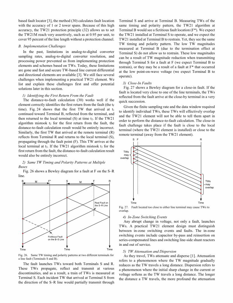
A. Measuring Distance-to-Fault Using Traveling Waves Fig. 24 shows a Bewley diagram for a fault at location F on

a line of length LL. The fault is M (km or mi) away from the local terminal (S) and LL – M (km or mi) away from the remote terminal (R). Consider another terminal (B) behind the local terminal. A TW line propagation time (TWLPT) is the time it takes for a TW to travel from one line terminal to the opposite terminal.

A TW launched at the fault point (F) arrives at the local terminal (S) at t1. Part of it reflects, travels back toward the fault, reflects back from the fault, and then returns to the local terminal (S) at t4. During the t4 – t1 time interval, the TW travels a distance of 2·M. We write the distance-velocity-time equation as follows:

2 ∙ M = (t4 − t1) ∙ PV (28)

where the propagation velocity, PV, is:

PV =LL

TWLPT (29)

Substituting (29) into (28) and solving for M, we obtain the key equation for calculating the distance-to-fault value:

M =LL2

t4 − t1TWLPT

(30)

Introducing a per-unit reach, TW21M, we use (30) to write the following fundamental operating equation for the TW21 underreaching distance element:

tF − t1

2 ∙ TWLPT< TW21M (31)

where: t1 is the arrival time of the very first TW, tF is the arrival time of the first return from the fault (t4 in Fig. 24).

S F R

t1

M LL – MtFAULT = 0

B

t2

t3

t4

t5

Time Time Time

Fig. 24. Bewley diagram for a fault on a transmission line.

To emphasize reliance of the TW21 on the measurement of time, we rewrite the TW21 operating equation as follows (see Fig. 25):

(tF − t1) < 2 ∙ TW21M ∙ TWLPT (32)

The left-hand side of (32) is the relay measurement. Responding only to TW arrival times, this measurement is very accurate because it is not affected by CT and PT ratio errors, transients, and signal distortions in the lower (kHz) frequency band. The TW21 element does not use line impedance data when calculating the operating signal (32), and therefore the operating signal is not affected by the finite accuracy of such line data.

TW Detection and Time-Stamping

Subsystem

tF – t1

Reach Setting

Directional Supervision (TW32)

Other Security Conditions

TW21–

+

Fig. 25. Simplified logic diagram of the TW21 element.

The right-hand side of (32) is a threshold fixed for any given application—a product of the line length expressed in the TW line propagation time, TWLPT, and the user-preferred per-unit reach setting, TW21M. When used in the single-ended TW-

based fault locator [3], the method (30) calculates fault location with the accuracy of 1 or 2 tower spans. Because of this high accuracy, the TW21 protection principle (32) allows us to set the TW21M reach very assertively, such as at 0.95 per unit, to cover 95 percent of the line length without a protection channel.

B. Implementation Challenges In the past, limitations in analog-to-digital converter

sampling rates, analog-to-digital converter resolution, and processing power prevented us from implementing protection elements and schemes based on TWs. Today, these limitations are gone and fast and secure TW-based line current differential and directional elements are available [3]. We still face several challenges when implementing a practical TW21 element. We list and explain these challenges first and offer potential solutions later in this section.

1) Identifying the First Return From the Fault The distance-to-fault calculation (30) works well if the

element correctly identifies the first return from the fault (the tF time). Fig. 24 shows that the first TW that arrived at t1 continued toward Terminal B, reflected from the terminal, and then returned to the local terminal (S) at time t2. If the TW21 algorithm mistook t2 for the first return from the fault, the distance-to-fault calculation result would be entirely incorrect. Similarly, the first TW that arrived at the remote terminal (R) reflects from Terminal R and returns to the local terminal (S), propagating through the fault point (F). This TW arrives at the local terminal at t3. If the TW21 algorithm mistook t3 for the first return from the fault, the distance-to-fault calculation result would also be entirely incorrect.

2) Same TW Timing and Polarity Patterns at Multiple Buses

Fig. 26 shows a Bewley diagram for a fault at F on the S–R line.

S F RMB

Time Time Time

F*M

Real Fault on the S–R Line

Fictitious Fault on the B–S Line

Fig. 26. Same TW timing and polarity patterns at two different terminals for a line fault (Terminals S and B).

The fault launches TWs toward both Terminals S and R. These TWs propagate, reflect and transmit at various discontinuities, and as a result, a train of TWs is measured at Terminal S. Each incident TW that arrived at Terminal S from the direction of the S–R line would partially transmit through

Terminal S and arrive at Terminal B. Measuring TWs of the same timing and polarity pattern, the TW21 algorithm at Terminal B would see a fictitious fault location (F*). We expect the TW21 installed at Terminal S to operate, and we expect the TW21 installed at Terminal B to restrain. Yet, they see the same TW timing and polarity pattern. The low TW magnitudes measured at Terminal B (due to the termination effect at Terminal S) do not allow us to restrain. These low magnitudes can be a result of TW magnitude reduction when transmitting through Terminal S for a fault at F (we expect Terminal B to restrain), or they may be a result of a fault at F* that occurred at the low point-on-wave voltage (we expect Terminal B to operate).

3) Close-In Faults Fig. 27 shows a Bewley diagram for a close-in fault. If the

fault is located very close to one of the line terminals, the TWs reflected from the fault arrive at the close-by terminal in a very quick succession.

Given the finite sampling rate and the data window required to identify individual TWs, these TWs will effectively overlap and the TW21 element will not be able to tell them apart in order to perform the distance-to-fault calculation. The close-in fault challenge takes place if the fault is close to the local terminal (where the TW21 element is installed) or close to the remote terminal (away from the TW21 element).

S F R

TimeTime

TWs may

overlap

TWs may overlap

Fig. 27. Fault located too close to either line terminal may cause TWs to overlap.

4) In-Zone Switching Events Any abrupt change in voltage, not only a fault, launches

TWs. A practical TW21 element design must distinguish between in-zone switching events and faults. The in-zone switching events include capacitor by-pass and reinsertion on series-compensated lines and switching line-side shunt reactors in and out of service.

5) TW Attenuation and Dispersion As they travel, TWs attenuate and disperse [1]. Attenuation

refers to a phenomenon where the TW magnitude gradually reduces as the TW travels a long distance. Dispersion refers to a phenomenon where the initial sharp change in the current or voltage softens as the TW travels a long distance. The longer the distance a TW travels, the more profound the attenuation

and dispersion, and the harder it gets to identify and time-stamp that TW. Consider a fault at 200 mi on a 220 mi line (Fig. 28). The first return from the fault is a TW that traveled 600 mi and reflected twice before arriving at the terminal. As a result, this TW can have a very low magnitude and may be considerably dispersed creating sensitivity and accuracy challenges for the TW21 element.

S F R

TimeTime

200 mi

200 mi

200 mi(1)

(2)

This TW Traveled 600 mi and Reflected Twice

200 mi

Fig. 28. TW21 element works with TWs that traveled long distances.

We use the following ideas to solve the above TW21 implementation challenges.

C. High-Fidelity Voltage Measurement A high-fidelity voltage signal is absolutely essential for the

TW21 protection element. High-fidelity voltage allows us to identify directionality of every single TW that we measure during a fault, i.e., we can tell if any given TW arrived from the direction of the line or from the area behind the terminal. Note that knowing the fault direction, such as by using any ultra-high-speed directional element, is not sufficient. For a forward fault, we still have TWs coming from the line direction as well as reflections from discontinuities behind the relay. High-fidelity voltage also allows us to separate the incident and reflected TWs, i.e., we can tell the magnitude, polarity, and shape of the TW that arrived at the terminal versus the TW that reflected from the terminal and traveled back toward the line. Separating the incident and reflected TWs allows a number of solutions to TW21 challenges as we explain later.

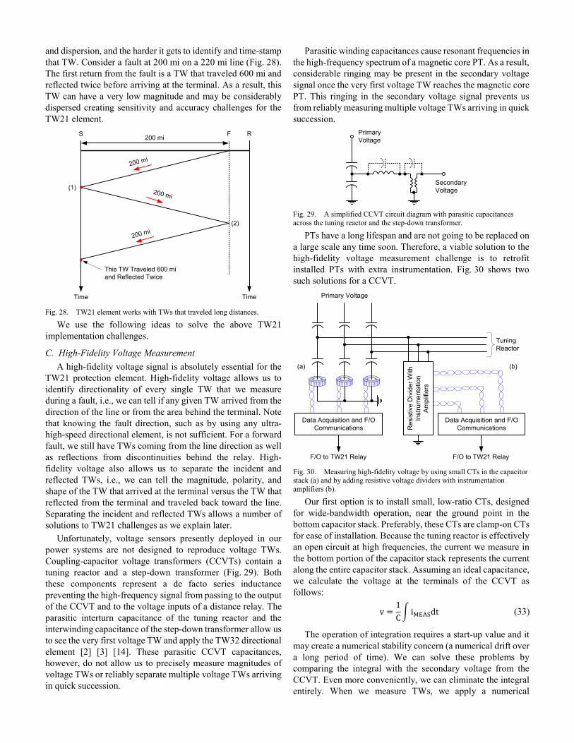
Unfortunately, voltage sensors presently deployed in our power systems are not designed to reproduce voltage TWs. Coupling-capacitor voltage transformers (CCVTs) contain a tuning reactor and a step-down transformer (Fig. 29). Both these components represent a de facto series inductance preventing the high-frequency signal from passing to the output of the CCVT and to the voltage inputs of a distance relay. The parasitic interturn capacitance of the tuning reactor and the interwinding capacitance of the step-down transformer allow us to see the very first voltage TW and apply the TW32 directional element [2] [3] [14]. These parasitic CCVT capacitances, however, do not allow us to precisely measure magnitudes of voltage TWs or reliably separate multiple voltage TWs arriving in quick succession.

Parasitic winding capacitances cause resonant frequencies in the high-frequency spectrum of a magnetic core PT. As a result, considerable ringing may be present in the secondary voltage signal once the very first voltage TW reaches the magnetic core PT. This ringing in the secondary voltage signal prevents us from reliably measuring multiple voltage TWs arriving in quick succession.

Primary Voltage

Secondary Voltage

Fig. 29. A simplified CCVT circuit diagram with parasitic capacitances across the tuning reactor and the step-down transformer.

PTs have a long lifespan and are not going to be replaced on a large scale any time soon. Therefore, a viable solution to the high-fidelity voltage measurement challenge is to retrofit installed PTs with extra instrumentation. Fig. 30 shows two such solutions for a CCVT.

Res

istiv

e D

ivid

er W

ith

Inst

rum

enta

tion

Ampl

ifier

s

Tuning Reactor

Data Acquisition and F/O Communications

F/O to TW21 Relay

Data Acquisition and F/O Communications

F/O to TW21 Relay

(a) (b)

Primary Voltage

Fig. 30. Measuring high-fidelity voltage by using small CTs in the capacitor stack (a) and by adding resistive voltage dividers with instrumentation amplifiers (b).

Our first option is to install small, low-ratio CTs, designed for wide-bandwidth operation, near the ground point in the bottom capacitor stack. Preferably, these CTs are clamp-on CTs for ease of installation. Because the tuning reactor is effectively an open circuit at high frequencies, the current we measure in the bottom portion of the capacitor stack represents the current along the entire capacitor stack. Assuming an ideal capacitance, we calculate the voltage at the terminals of the CCVT as follows:

v =1C� iMEASdt (33)

The operation of integration requires a start-up value and it may create a numerical stability concern (a numerical drift over a long period of time). We can solve these problems by comparing the integral with the secondary voltage from the CCVT. Even more conveniently, we can eliminate the integral entirely. When we measure TWs, we apply a numerical

differentiator-smoother filter [1]. Instead of treating voltage with the numerical differentiator-smoother, we can treat the measured current in the CCVT stack with a numerical smoother filter and obtain the same result. By doing so, we effectively allow the capacitor to differentiate the voltage (the signal we are interested in) into the current (the signal we measure).

Our second option is to install a low-burden fused resistive divider across the bottom stack of a CCVT and use instrumentation amplifiers to acquire the voltage signal with high fidelity.

When using either of the two solutions, we install our data acquisition system close to the CCVT in order to maximize integrity of these low-energy wide-bandwidth signals. We then use a direct fiber-optic (F/O) connection to deliver the samples representing the voltage signal to the relay.

D. Identifying Key TW Reflections for the Distance-to-Fault Measurement

Having access to a high-fidelity voltage signal, we detect directionality of every TW that arrives at the line terminal. With reference to Fig. 24, we know t2 is the time of arrival of a TW that came from behind the relay, and therefore it is not the first return from the fault. However, TW directionality itself does not entirely solve the problem of identifying the right reflection for the distance-to-fault calculations (30).

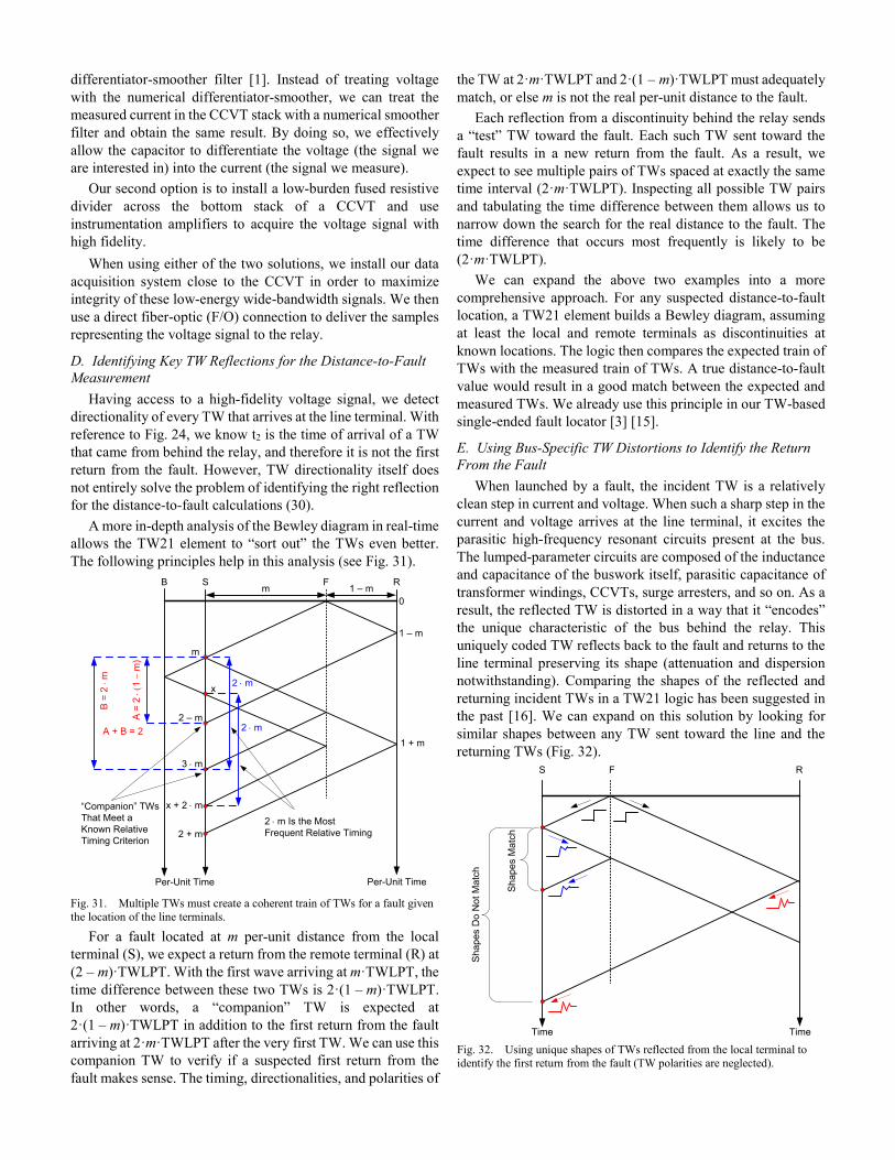
A more in-depth analysis of the Bewley diagram in real-time allows the TW21 element to “sort out” the TWs even better. The following principles help in this analysis (see Fig. 31).

S F Rm 1 – mB

Per-Unit Time

1 – m

m

2 – m

3 ⋅ m

Per-Unit Time

x

x + 2 ⋅ m

2 + m

2 ⋅ m

2 ⋅ m

A =

2 ⋅ (

1 −

m)

B =

2 ⋅ m

A + B = 2

“Companion” TWs That Meet a Known Relative Timing Criterion

2 ⋅ m Is the Most Frequent Relative Timing

1 + m

0

Fig. 31. Multiple TWs must create a coherent train of TWs for a fault given the location of the line terminals.

For a fault located at m per-unit distance from the local terminal (S), we expect a return from the remote terminal (R) at (2 – m)·TWLPT. With the first wave arriving at m·TWLPT, the time difference between these two TWs is 2·(1 – m)·TWLPT. In other words, a “companion” TW is expected at 2·(1 – m)·TWLPT in addition to the first return from the fault arriving at 2·m·TWLPT after the very first TW. We can use this companion TW to verify if a suspected first return from the fault makes sense. The timing, directionalities, and polarities of

the TW at 2·m·TWLPT and 2·(1 – m)·TWLPT must adequately match, or else m is not the real per-unit distance to the fault.

Each reflection from a discontinuity behind the relay sends a “test” TW toward the fault. Each such TW sent toward the fault results in a new return from the fault. As a result, we expect to see multiple pairs of TWs spaced at exactly the same time interval (2·m·TWLPT). Inspecting all possible TW pairs and tabulating the time difference between them allows us to narrow down the search for the real distance to the fault. The time difference that occurs most frequently is likely to be (2·m·TWLPT).

We can expand the above two examples into a more comprehensive approach. For any suspected distance-to-fault location, a TW21 element builds a Bewley diagram, assuming at least the local and remote terminals as discontinuities at known locations. The logic then compares the expected train of TWs with the measured train of TWs. A true distance-to-fault value would result in a good match between the expected and measured TWs. We already use this principle in our TW-based single-ended fault locator [3] [15].

E. Using Bus-Specific TW Distortions to Identify the Return From the Fault

When launched by a fault, the incident TW is a relatively clean step in current and voltage. When such a sharp step in the current and voltage arrives at the line terminal, it excites the parasitic high-frequency resonant circuits present at the bus. The lumped-parameter circuits are composed of the inductance and capacitance of the buswork itself, parasitic capacitance of transformer windings, CCVTs, surge arresters, and so on. As a result, the reflected TW is distorted in a way that it “encodes” the unique characteristic of the bus behind the relay. This uniquely coded TW reflects back to the fault and returns to the line terminal preserving its shape (attenuation and dispersion notwithstanding). Comparing the shapes of the reflected and returning incident TWs in a TW21 logic has been suggested in the past [16]. We can expand on this solution by looking for similar shapes between any TW sent toward the line and the returning TWs (Fig. 32).

S F R

Time

Shap

es M

atch

Shap

es D

o N

ot M

atch

Time Fig. 32. Using unique shapes of TWs reflected from the local terminal to identify the first return from the fault (TW polarities are neglected).

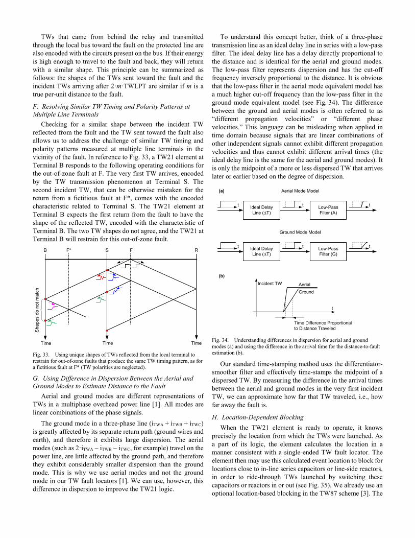
TWs that came from behind the relay and transmitted through the local bus toward the fault on the protected line are also encoded with the circuits present on the bus. If their energy is high enough to travel to the fault and back, they will return with a similar shape. This principle can be summarized as follows: the shapes of the TWs sent toward the fault and the incident TWs arriving after 2·m·TWLPT are similar if m is a true per-unit distance to the fault.

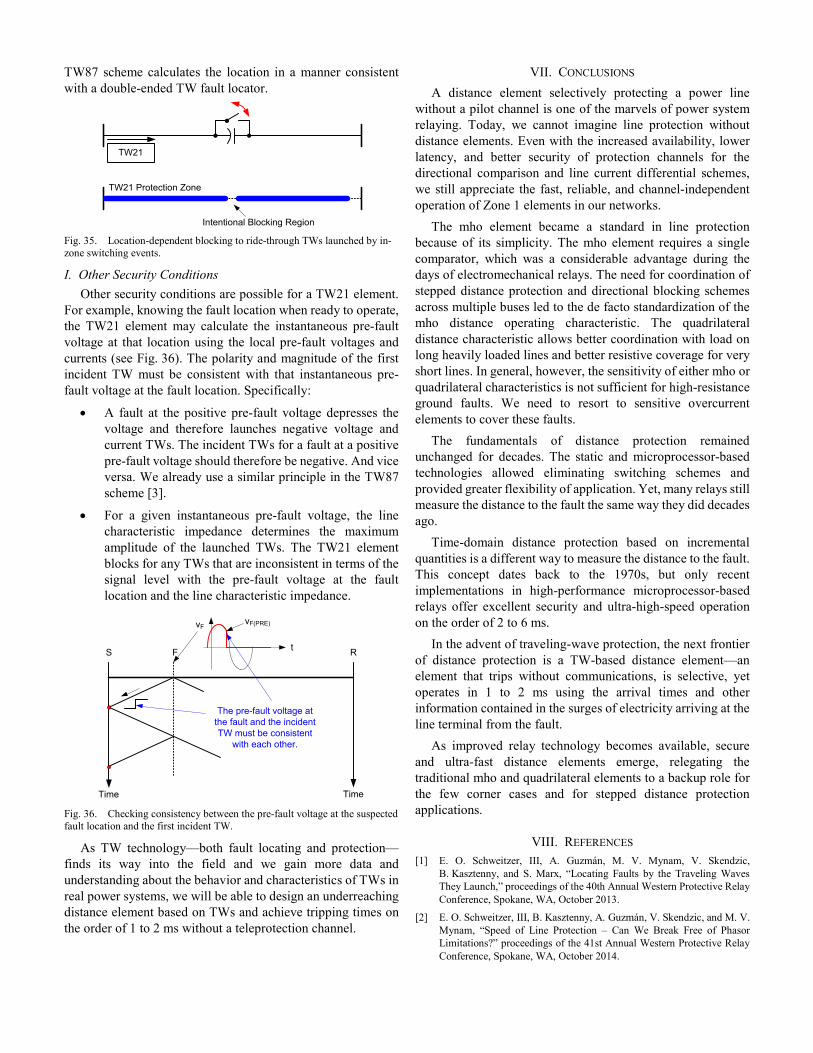
F. Resolving Similar TW Timing and Polarity Patterns at Multiple Line Terminals

Checking for a similar shape between the incident TW reflected from the fault and the TW sent toward the fault also allows us to address the challenge of similar TW timing and polarity patterns measured at multiple line terminals in the vicinity of the fault. In reference to Fig. 33, a TW21 element at Terminal B responds to the following operating conditions for the out-of-zone fault at F. The very first TW arrives, encoded by the TW transmission phenomenon at Terminal S. The second incident TW, that can be otherwise mistaken for the return from a fictitious fault at F*, comes with the encoded characteristic related to Terminal S. The TW21 element at Terminal B expects the first return from the fault to have the shape of the reflected TW, encoded with the characteristic of Terminal B. The two TW shapes do not agree, and the TW21 at Terminal B will restrain for this out-of-zone fault.

S F R

Time Time

Shap

es d

o no

t mat

ch

B

Time

F*

Fig. 33. Using unique shapes of TWs reflected from the local terminal to restrain for out-of-zone faults that produce the same TW timing pattern, as for a fictitious fault at F* (TW polarities are neglected).

G. Using Difference in Dispersion Between the Aerial and Ground Modes to Estimate Distance to the Fault

Aerial and ground modes are different representations of TWs in a multiphase overhead power line [1]. All modes are linear combinations of the phase signals.

The ground mode in a three-phase line (iTWA + iTWB + iTWC) is greatly affected by its separate return path (ground wires and earth), and therefore it exhibits large dispersion. The aerial modes (such as 2·iTWA – iTWB – iTWC, for example) travel on the power line, are little affected by the ground path, and therefore they exhibit considerably smaller dispersion than the ground mode. This is why we use aerial modes and not the ground mode in our TW fault locators [1]. We can use, however, this difference in dispersion to improve the TW21 logic.

To understand this concept better, think of a three-phase transmission line as an ideal delay line in series with a low-pass filter. The ideal delay line has a delay directly proportional to the distance and is identical for the aerial and ground modes. The low-pass filter represents dispersion and has the cut-off frequency inversely proportional to the distance. It is obvious that the low-pass filter in the aerial mode equivalent model has a much higher cut-off frequency than the low-pass filter in the ground mode equivalent model (see Fig. 34). The difference between the ground and aerial modes is often referred to as “different propagation velocities” or “different phase velocities.” This language can be misleading when applied in time domain because signals that are linear combinations of other independent signals cannot exhibit different propagation velocities and thus cannot exhibit different arrival times (the ideal delay line is the same for the aerial and ground modes). It is only the midpoint of a more or less dispersed TW that arrives later or earlier based on the degree of dispersion.

Ideal Delay Line (∆T)

Aerial Mode Model

Low-Pass Filter (A)

tt t

Ideal Delay Line (∆T)

Ground Mode Model

Low-Pass Filter (G)

tt t

t

Incident TW

Time Difference Proportional to Distance Traveled

AerialGround

(b)

(a)

Fig. 34. Understanding differences in dispersion for aerial and ground modes (a) and using the difference in the arrival time for the distance-to-fault estimation (b).

Our standard time-stamping method uses the differentiator-smoother filter and effectively time-stamps the midpoint of a dispersed TW. By measuring the difference in the arrival times between the aerial and ground modes in the very first incident TW, we can approximate how far that TW traveled, i.e., how far away the fault is.

H. Location-Dependent Blocking When the TW21 element is ready to operate, it knows

precisely the location from which the TWs were launched. As a part of its logic, the element calculates the location in a manner consistent with a single-ended TW fault locator. The element then may use this calculated event location to block for locations close to in-line series capacitors or line-side reactors, in order to ride-through TWs launched by switching these capacitors or reactors in or out (see Fig. 35). We already use an optional location-based blocking in the TW87 scheme [3]. The

TW87 scheme calculates the location in a manner consistent with a double-ended TW fault locator.

TW21

TW21 Protection Zone

Intentional Blocking Region Fig. 35. Location-dependent blocking to ride-through TWs launched by in-zone switching events.

I. Other Security Conditions Other security conditions are possible for a TW21 element.

For example, knowing the fault location when ready to operate, the TW21 element may calculate the instantaneous pre-fault voltage at that location using the local pre-fault voltages and currents (see Fig. 36). The polarity and magnitude of the first incident TW must be consistent with that instantaneous pre-fault voltage at the fault location. Specifically:

• A fault at the positive pre-fault voltage depresses the voltage and therefore launches negative voltage and current TWs. The incident TWs for a fault at a positive pre-fault voltage should therefore be negative. And vice versa. We already use a similar principle in the TW87 scheme [3].

• For a given instantaneous pre-fault voltage, the line characteristic impedance determines the maximum amplitude of the launched TWs. The TW21 element blocks for any TWs that are inconsistent in terms of the signal level with the pre-fault voltage at the fault location and the line characteristic impedance.

S F R

Time Time

vFvF(PRE)

t

The pre-fault voltage at the fault and the incident TW must be consistent

with each other.

Fig. 36. Checking consistency between the pre-fault voltage at the suspected fault location and the first incident TW.

As TW technology—both fault locating and protection—finds its way into the field and we gain more data and understanding about the behavior and characteristics of TWs in real power systems, we will be able to design an underreaching distance element based on TWs and achieve tripping times on the order of 1 to 2 ms without a teleprotection channel.

VII. CONCLUSIONS A distance element selectively protecting a power line

without a pilot channel is one of the marvels of power system relaying. Today, we cannot imagine line protection without distance elements. Even with the increased availability, lower latency, and better security of protection channels for the directional comparison and line current differential schemes, we still appreciate the fast, reliable, and channel-independent operation of Zone 1 elements in our networks.

The mho element became a standard in line protection because of its simplicity. The mho element requires a single comparator, which was a considerable advantage during the days of electromechanical relays. The need for coordination of stepped distance protection and directional blocking schemes across multiple buses led to the de facto standardization of the mho distance operating characteristic. The quadrilateral distance characteristic allows better coordination with load on long heavily loaded lines and better resistive coverage for very short lines. In general, however, the sensitivity of either mho or quadrilateral characteristics is not sufficient for high-resistance ground faults. We need to resort to sensitive overcurrent elements to cover these faults.

The fundamentals of distance protection remained unchanged for decades. The static and microprocessor-based technologies allowed eliminating switching schemes and provided greater flexibility of application. Yet, many relays still measure the distance to the fault the same way they did decades ago.

Time-domain distance protection based on incremental quantities is a different way to measure the distance to the fault. This concept dates back to the 1970s, but only recent implementations in high-performance microprocessor-based relays offer excellent security and ultra-high-speed operation on the order of 2 to 6 ms.

In the advent of traveling-wave protection, the next frontier of distance protection is a TW-based distance element—an element that trips without communications, is selective, yet operates in 1 to 2 ms using the arrival times and other information contained in the surges of electricity arriving at the line terminal from the fault.

As improved relay technology becomes available, secure and ultra-fast distance elements emerge, relegating the traditional mho and quadrilateral elements to a backup role for the few corner cases and for stepped distance protection applications.

VIII. REFERENCES [1] E. O. Schweitzer, III, A. Guzmán, M. V. Mynam, V. Skendzic,

B. Kasztenny, and S. Marx, “Locating Faults by the Traveling Waves They Launch,” proceedings of the 40th Annual Western Protective Relay Conference, Spokane, WA, October 2013.

[2] E. O. Schweitzer, III, B. Kasztenny, A. Guzmán, V. Skendzic, and M. V. Mynam, “Speed of Line Protection – Can We Break Free of Phasor Limitations?” proceedings of the 41st Annual Western Protective Relay Conference, Spokane, WA, October 2014.

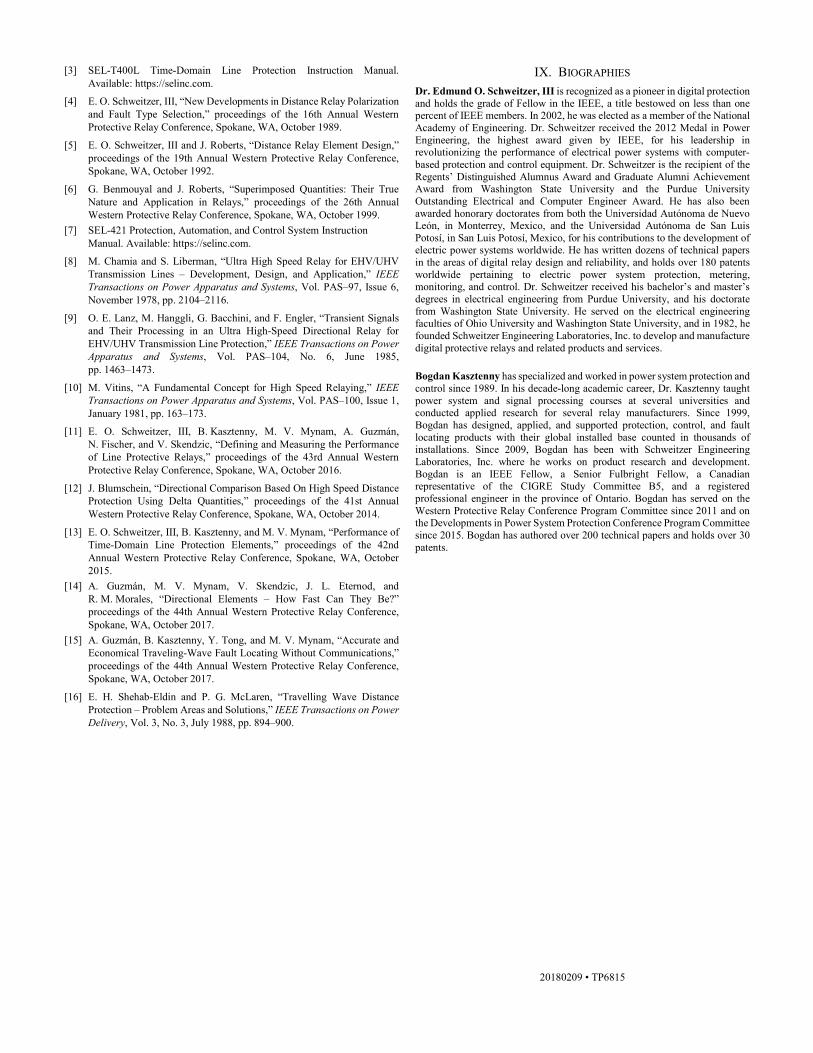
[3] SEL-T400L Time-Domain Line Protection Instruction Manual. Available: https://selinc.com.

[4] E. O. Schweitzer, III, “New Developments in Distance Relay Polarization and Fault Type Selection,” proceedings of the 16th Annual Western Protective Relay Conference, Spokane, WA, October 1989.

[5] E. O. Schweitzer, III and J. Roberts, “Distance Relay Element Design,” proceedings of the 19th Annual Western Protective Relay Conference, Spokane, WA, October 1992.

[6] G. Benmouyal and J. Roberts, “Superimposed Quantities: Their True Nature and Application in Relays,” proceedings of the 26th Annual Western Protective Relay Conference, Spokane, WA, October 1999.

[7] SEL-421 Protection, Automation, and Control System Instruction Manual. Available: https://selinc.com.

[8] M. Chamia and S. Liberman, “Ultra High Speed Relay for EHV/UHV Transmission Lines – Development, Design, and Application,” IEEE Transactions on Power Apparatus and Systems, Vol. PAS–97, Issue 6, November 1978, pp. 2104–2116.

[9] O. E. Lanz, M. Hanggli, G. Bacchini, and F. Engler, “Transient Signals and Their Processing in an Ultra High-Speed Directional Relay for EHV/UHV Transmission Line Protection,” IEEE Transactions on Power Apparatus and Systems, Vol. PAS–104, No. 6, June 1985, pp. 1463–1473.

[10] M. Vitins, “A Fundamental Concept for High Speed Relaying,” IEEE Transactions on Power Apparatus and Systems, Vol. PAS–100, Issue 1, January 1981, pp. 163–173.

[11] E. O. Schweitzer, III, B. Kasztenny, M. V. Mynam, A. Guzmán, N. Fischer, and V. Skendzic, “Defining and Measuring the Performance of Line Protective Relays,” proceedings of the 43rd Annual Western Protective Relay Conference, Spokane, WA, October 2016.

[12] J. Blumschein, “Directional Comparison Based On High Speed Distance Protection Using Delta Quantities,” proceedings of the 41st Annual Western Protective Relay Conference, Spokane, WA, October 2014.

[13] E. O. Schweitzer, III, B. Kasztenny, and M. V. Mynam, “Performance of Time-Domain Line Protection Elements,” proceedings of the 42nd Annual Western Protective Relay Conference, Spokane, WA, October 2015.

[14] A. Guzmán, M. V. Mynam, V. Skendzic, J. L. Eternod, and R. M. Morales, “Directional Elements – How Fast Can They Be?” proceedings of the 44th Annual Western Protective Relay Conference, Spokane, WA, October 2017.

[15] A. Guzmán, B. Kasztenny, Y. Tong, and M. V. Mynam, “Accurate and Economical Traveling-Wave Fault Locating Without Communications,” proceedings of the 44th Annual Western Protective Relay Conference, Spokane, WA, October 2017.

[16] E. H. Shehab-Eldin and P. G. McLaren, “Travelling Wave Distance Protection – Problem Areas and Solutions,” IEEE Transactions on Power Delivery, Vol. 3, No. 3, July 1988, pp. 894–900.

IX. BIOGRAPHIES Dr. Edmund O. Schweitzer, III is recognized as a pioneer in digital protection and holds the grade of Fellow in the IEEE, a title bestowed on less than one percent of IEEE members. In 2002, he was elected as a member of the National Academy of Engineering. Dr. Schweitzer received the 2012 Medal in Power Engineering, the highest award given by IEEE, for his leadership in revolutionizing the performance of electrical power systems with computer-based protection and control equipment. Dr. Schweitzer is the recipient of the Regents’ Distinguished Alumnus Award and Graduate Alumni Achievement Award from Washington State University and the Purdue University Outstanding Electrical and Computer Engineer Award. He has also been awarded honorary doctorates from both the Universidad Autónoma de Nuevo León, in Monterrey, Mexico, and the Universidad Autónoma de San Luis Potosí, in San Luis Potosí, Mexico, for his contributions to the development of electric power systems worldwide. He has written dozens of technical papers in the areas of digital relay design and reliability, and holds over 180 patents worldwide pertaining to electric power system protection, metering, monitoring, and control. Dr. Schweitzer received his bachelor’s and master’s degrees in electrical engineering from Purdue University, and his doctorate from Washington State University. He served on the electrical engineering faculties of Ohio University and Washington State University, and in 1982, he founded Schweitzer Engineering Laboratories, Inc. to develop and manufacture digital protective relays and related products and services.

Bogdan Kasztenny has specialized and worked in power system protection and control since 1989. In his decade-long academic career, Dr. Kasztenny taught power system and signal processing courses at several universities and conducted applied research for several relay manufacturers. Since 1999, Bogdan has designed, applied, and supported protection, control, and fault locating products with their global installed base counted in thousands of installations. Since 2009, Bogdan has been with Schweitzer Engineering Laboratories, Inc. where he works on product research and development. Bogdan is an IEEE Fellow, a Senior Fulbright Fellow, a Canadian representative of the CIGRE Study Committee B5, and a registered professional engineer in the province of Ontario. Bogdan has served on the Western Protective Relay Conference Program Committee since 2011 and on the Developments in Power System Protection Conference Program Committee since 2015. Bogdan has authored over 200 technical papers and holds over 30 patents.

20180209 • TP6815