Distance based Service Level Agreement assessment

Distance based Service Level Agreement assessment∗

Rene Serral-Gracia, Yann Labit Jordi Domingo-Pascual, Philippe OwezarskiAdvanced Broadband Communications Centre, Technical University ofCatalunya (UPC), Spain

E-mail:{rserral, jordid}@ac.upc.eduLaboratoire d’Analyse et d’Architecture des Systemes (LAAS), France

E-mail:{ylabit, owe}@laas.fr

September 8, 2008

Abstract

On-line end-to-end Service Level Agreement (SLA) monitoring is of key importance nowadays. For this purpose,past recent researches focused on measuring (when possible) or estimating (most of the times) network QoS orperformance parameters. Up to now, attempts to provide accurate techniques for estimating such parameters failed.In addition, live reporting of the estimated network status requires a huge amount of resources, and lead to unscalablesystems.

The originality of the contribution presented in this paper relies on the statement that the accurate estimation ofnetwork QoS parameters is absolutely not required in most cases: specifically it is sufficient to be aware of servicedisruptions, i.e. when the QoS provided by the network collapses. For this purpose, two different algorithms fordisruption detection of network services are proposed, each one having its own advantages. The two alternative arebased on the use of Kullback-Leibler Divergence and the well-known Hausdorff Distance algorithm, which are veryefficient comparison algorithms that use respectively entropies and geometric distances. The two algorithms morespecifically work on simple to measure time series, i.e. received inter-packet arrival times. In addition of efficientlydetecting network QoS disruptions, both algorithms, also drastically reduce the required resources, and the overheadproduced by the traffic collection for scalable SLA monitoring systems.

The validity of the proposal is verified by comparing the two alternatives, both in terms of accuracy and consumedresources in a real testbed, using different traffic profiles generated by several applications.

1 IntroductionOn-line end-to-end Service Level Agreement (SLA) monitoring is of key importance nowadays. Both ISP and

customers want to know at any time the quality of the network services, and whether it is respecting the contractedSLA. For this purpose, classical approaches for SLA assessment [1, 2, 3, 4] focused on accurately measuring (whenpossible) or estimating (most of the times) network QoS or performance parameters such as One Way Delay (OWD),Inter Packet Delay Variation (IPDV), Available BandWidth (ABW), Packet Loss Ratio (PLR), etc. Up to now, attemptsto provide accurate techniques for estimating such parameters failed (e.g. for ABW, estimation accuracy in realenvironments presents error rates greater than 50% [5]). This is essentially due to network variability, non-periodictraffic, and different effects of network anomalies which make SLA assessment a challenging problem.

In addition, computing the metrics presents several other drawbacks:

• Estimating the metrics implies to gather distributed information about the traffic and the synchronisation amongthe involved entities. Such control traffic is an important bottleneck of any solution using this approach [1].

• Computing the metrics requires multiple capture points. And in the case of using active probing a traffic gener-ation station located in some advantage point.

∗This work was partially funded by IST under contract 6FP-004503 (IST-EuQoS), NoE-038423 (Content), MCyT (Spanish Ministry of Scienceand Technology) under contract TSI 2005-07520-C03-02 and the CIRIT (Catalan Research Council) under contract 2005 SGR 00481.

1

Therefore, such systems suffer from large scalability issues.In such context, we do not intend to improve the accuracy on the QoS metric estimation. The originality of the

contribution presented in this paper relies on the statement that the accurate estimation of network QoS parametersis absolutely not required in most cases: specifically it is sufficient to be aware of service disruptions, i.e. when theQoS provided by the network collapses. In our original approach we just focus on the actual scalable detection andreporting of any potential violation of the SLA in the network. For this purpose, we propose in this paper a newapproach which:

1. Works as much as possible with a single point of analysis.

2. Computes data very efficiently in order to have a scalable system.

3. Relies on the use of existing correlation between measured parameters and network quality.

We then propose to use Inter Packet Arrival Time (IPAT) because it complies with the above restrictions: IPATscan be easily computed at destination by getting the reception timestamps of the packets; IPAT computation onlyinvolves a subtraction of two integers (timestamps). Finally, and this is what we want to prove in the rest of the paper,it exists a strong correlation between IPAT distribution and network performance: it was demonstrated by previouswork that IPATs are tightly correlated with network congestion [6, 7]. In this work, we bring this correlation one stepfurther by mapping these IPATs with the actual network conditions by using some information about the real metrics.In particular, our proposal relies on statistical analysis of the IPATs, with the goal of detecting changes on the networkstatus. This is done by comparing different IPAT distributions using well-known algorithms, such as Kullback-LeiblerDivergence and Hausdorff Distance.

We validate our solution with different real scenarios, first over a controlled testbed with customisable networkconditions, and later with an European wide scenario with 12 different local testbeds and access technologies. Inboth scenarios we performed a broad range of tests, from synthetic generated UDP traffic, to audio and video flowsgenerated by a real video streaming application.

Our results confirm the great adaptability and accurate detection of the different SLA violations found in our traces,all accomplished by reducing the resource usage down to a∼ 11%, with an accuracy of≥ 85% compared to the perfectknowledge of the SLA violations using real video streaming traffic in our testbed.

The rest of the paper is structured as follows. Next section details some related work. After this, outlining the maincontribution of this paper, we detail the proposed distance algorithms. In Section 5 we present the used methodologyin order to perform the on-line SLA Assessment. After this the paper discusses the different tests and their conditionsin order to evaluate the proposal. Section 8 details the evaluation results. Before concluding we discuss the feasibilityof implementing our solution in a real network, and finally in Section 11 we conclude and explain the open issues forfuture work.

2 Related WorkIn the active traffic analysis area, SLA Assessment has been previously studied. Some important work has been

performed by Barford et al. in [8], where the authors highlight the limitations of packet loss estimation using activeprobes, compared to the ones found via SNMP in commercial routers. This work is continued by Sommers et al. in [9],where the authors improve the loss estimation of classical Poisson-modulated probing mechanisms by presentingBadabing, a dynamic active tool that improves accuracy depending on the resources used for the estimation. Morerecently, in [4] Sommers et al. gather together all the above knowledge, and present SLAm, another active probingtool, which implements innovative packet loss, delay, and delay variation estimation techniques for SLA assessment.In all this research, the authors stress the need of proper metric estimation in order to lead to correct SLA assessment.Our work differs from this in the sense that our methodology does not focus on accurate metric estimation, but ratherin the search for relevant packet information to infer the network quality. Moreover, we use a passive traffic analysisapproach against the active solution adopted by the mentioned previous work.

Regarding passive traffic analysis, some research has been done in our previous work [1,2], in which we proposed adistributed infrastructure, for inferring the network quality by extracting the performance metrics from detailed packetinformation. The metric computation is centralised and requires several collection points on the edges of the networkthat send packet information (timestamps, etc.) to the central entity, with the consequent use of bandwidth due to this,so called, control traffic. Such received information is used by the central entity to compute the flow’s network metrics

2

(OWD, IPDV and PLR). In this paper, we use this mechanism as method for acquiring perfect knowledge about thenetwork status for our SLA assessment algorithm.

The main contribution of this work is the utilisation of two different algorithms in order to infer SLA violations.The first algorithm we study is Kullback-Leibler Divergence, which has been used before for instance in [10] toperform anomaly detection based on destination ports. The second algorithm we use is called Hausdorff Distance. Itwas used many times in image pattern recognition, and lately in networking, as in [11] for instance.

3 Background: IPAT and anomaliesThis section aims at showing empirically the relation between changes on IPAT and OWDs. In the past some

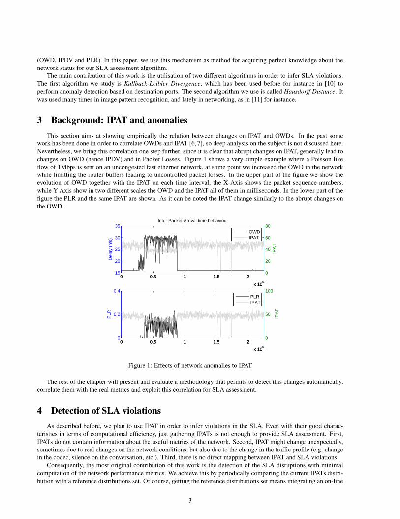
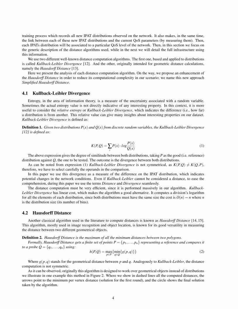
work has been done in order to correlate OWDs and IPAT [6, 7], so deep analysis on the subject is not discussed here.Nevertheless, we bring this correlation one step further, since it is clear that abrupt changes on IPAT, generally lead tochanges on OWD (hence IPDV) and in Packet Losses. Figure 1 shows a very simple example where a Poisson likeflow of 1Mbps is sent on an uncongested fast ethernet network, at some point we increased the OWD in the networkwhile limitting the router buffers leading to uncontrolled packet losses. In the upper part of the figure we show theevolution of OWD together with the IPAT on each time interval, the X-Axis shows the packet sequence numbers,while Y-Axis show in two different scales the OWD and the IPAT all of them in milliseconds. In the lower part of thefigure the PLR and the same IPAT are shown. As it can be noted the IPAT change similarly to the abrupt changes onthe OWD.

0 0.5 1 1.5 2

x 105

15

20

25

30

35Inter Packet Arrival time behaviour

Del

ay (

ms)

0 0.5 1 1.5 2

x 105

0

20

40

60

80

IPA

T

OWDIPAT

0 0.5 1 1.5 2

x 105

0

0.2

0.4

PLR

0 0.5 1 1.5 2

x 105

0

50

100

IPA

T

PLRIPAT

Figure 1: Effects of network anomalies to IPAT

The rest of the chapter will present and evaluate a methodology that permits to detect this changes automatically,correlate them with the real metrics and exploit this correlation for SLA assessment.

4 Detection of SLA violationsAs described before, we plan to use IPAT in order to infer violations in the SLA. Even with their good charac-

teristics in terms of computational efficiency, just gathering IPATs is not enough to provide SLA assessment. First,IPATs do not contain information about the useful metrics of the network. Second, IPAT might change unexpectedly,sometimes due to real changes on the network conditions, but also due to the change in the traffic profile (e.g. changein the codec, silence on the conversation, etc.). Third, there is no direct mapping between IPAT and SLA violations.

Consequently, the most original contribution of this work is the detection of the SLA disruptions with minimalcomputation of the network performance metrics. We achieve this by periodically comparing the current IPATs distri-bution with a reference distributions set. Of course, getting the reference distributions set means integrating an on-line

3

training process which records all new IPAT distributions observed on the network. It also makes, in the same time,the link between each of these new IPAT distributions and the current QoS parameters (by measuring them). Then,each IPATs distribution will be associated to a particular QoS level of the network. Then, in this section we focus onthe generic description of the distance algorithms used, while in the next we will detail the full infrastructure usingthis information.

We use two different well-known distance computation algorithms. The first one, based and applied to distributionsis called Kullback-Leibler Divergence [12]. And the other, originally intended for geometric distance calculations,namely the Hausdorff Distance [13].

Here we present the analysis of each distance computation algorithm. On the way, we propose an enhancement ofthe Hausdorff Distance in order to reduce its computational complexity in our scenario; we name this new approachSimplified Hausdorff Distance.

4.1 Kullback-Leibler DivergenceEntropy, in the area of information theory, is a measure of the uncertainty associated with a random variable.

Sometimes the actual entropy value is not directly indicative of any interesting property. In this context, it is moreuseful to consider the relative entropy or Kullback-Leibler Divergence, which indicates the difference (i.e., how far)a distribution is from another. This relative value can give many insights about interesting properties on our dataset.Kullback-Leibler Divergence is defined as:

Definition 1. Given two distributions P(x) and Q(x) from discrete random variables, the Kullback-Leibler Divergence[12] is defined as:

K(P,Q) = ∑i

P(x) · logP(x)Q(x)

(1)

The above expression gives the degree of similitude between both distributions, taking P as the good (i.e. reference)distribution against Q, the one to be tested. The outcome is the divergence between both distributions.

As can be noted from expression (1) Kullback-Leibler Divergence is not symmetrical, as K(P,Q) 6= K(Q,P),therefore, we have to select carefully the operands in the comparison.

In this paper we use this divergence as a measure of the difference on the IPAT distribution, which indicatespotential changes in the network conditions. Even if Kullback-Leibler cannot be considered a distance, to ease thecomprehension, during this paper we use the terms Distance and Divergence seamlessly.

The distance computation must be very efficient, since it is performed massively in our algorithm. Kullback-Leibler Divergence has linear cost, which makes the algorithm a good alternative. It computes a division’s logarithmfor all the elements of each distribution, since both distributions must have the same size the cost is O(n) = n where nis the distribution size (its number of bins).

4.2 Hausdorff DistanceAnother classical algorithm used in the literature to compute distances is known as Hausdorff Distance [14, 15].

This algorithm, mostly used in image recognition and object location, is known for its good versatility in measuringthe distance between two different geometrical objects.

Definition 2. Hausdorff Distance is the maximum of all the minimum distances between two polygons.Formally, Hausdorff Distance gets a finite set of points P = {p1, . . . , pn} representing a reference and compares it

to a probe Q = {q1, . . . ,qn} using:h(P,Q) = max

p∈P{min

q∈Q{g(p,q)}} (2)

Where g(p,q) stands for the geometrical distance between p and q. Analogously to Kullback-Leibler, the distancecomputation is not symmetric.

As it can be observed, originally this algorithm is designed to work over geometrical objects instead of distributionswe illustrate in one example this method in Figure 2. Where we show in dashed lines all the computed distances, thearrows point to the minimum per vertex distance (solution for the first round), and the circle shows the final solutiontaken by the algorithm.

4

a

b

c

1

2

3

Figure 2: Hausdorff Distance example

The efficiency, taken as computational cost is worse than. Kullback-Leibler Divergence Here we have to get theminimum distance from one element of P towards all the elements of Q, hence the cost is O(n) = nm where n is thesize of P and m is Q’s. In general we can assume that n≈ m, thus O(n) = n2.

This complexity for an on-line algorithm as the one we are proposing in this work represents a bottleneck on thesystem, but in general, as we will see in the evaluation section, Hausdorff Distance uses less network resources thanKullback-Leibler. Therefore, it is an interesting alternative in our environment.

4.3 The Simplified Hausdorff DistanceHausdorff Distance was designed in order to operate in the geometric plane, but we use distributions instead of

polygons, which allows us to reduce the algorithm’s complexity.Hausdorff Distance basically compares all the elements of a set with all the elements of the other. Although, when

working with distributions, there is a new dimension that does not exist on the geometrical plane, namely the bin size.Therefore, to reduce the computational cost, we only need to compare similar bins (in position and value) opposed tothe “all-against-all” policy of the original algorithm, this differences are illustrated in Figure 3.

2 4 6 80

0.2

0.4

2 4 6 80

0.2

0.4

2 4 6 80

0.2

0.4

0 2 4 6 80

0.2

0.4

0.6

0.8. . .

Figure 3: Hausdorff and Direct Hausdorff Distance differences

Hence, we define the Direct Hausdorff Distance as:

5

Definition 3. Let’s define o as the bin offset threshold, and P,Q two distributions, where P is the reference and Q theacquired distribution, with n and m elements respectively. We define the “Simplified Hausdorff Distance” as:

HD(P,Q) = maxi=1...n

{i+ominj=i−o{g(Pi,Q j)}} (3)

With this enhancement, the Simplified Hausdorff Distance has O(n) = n, linear cost for small values of o (0≤ o≤n), which in fact are the most useful in our context.

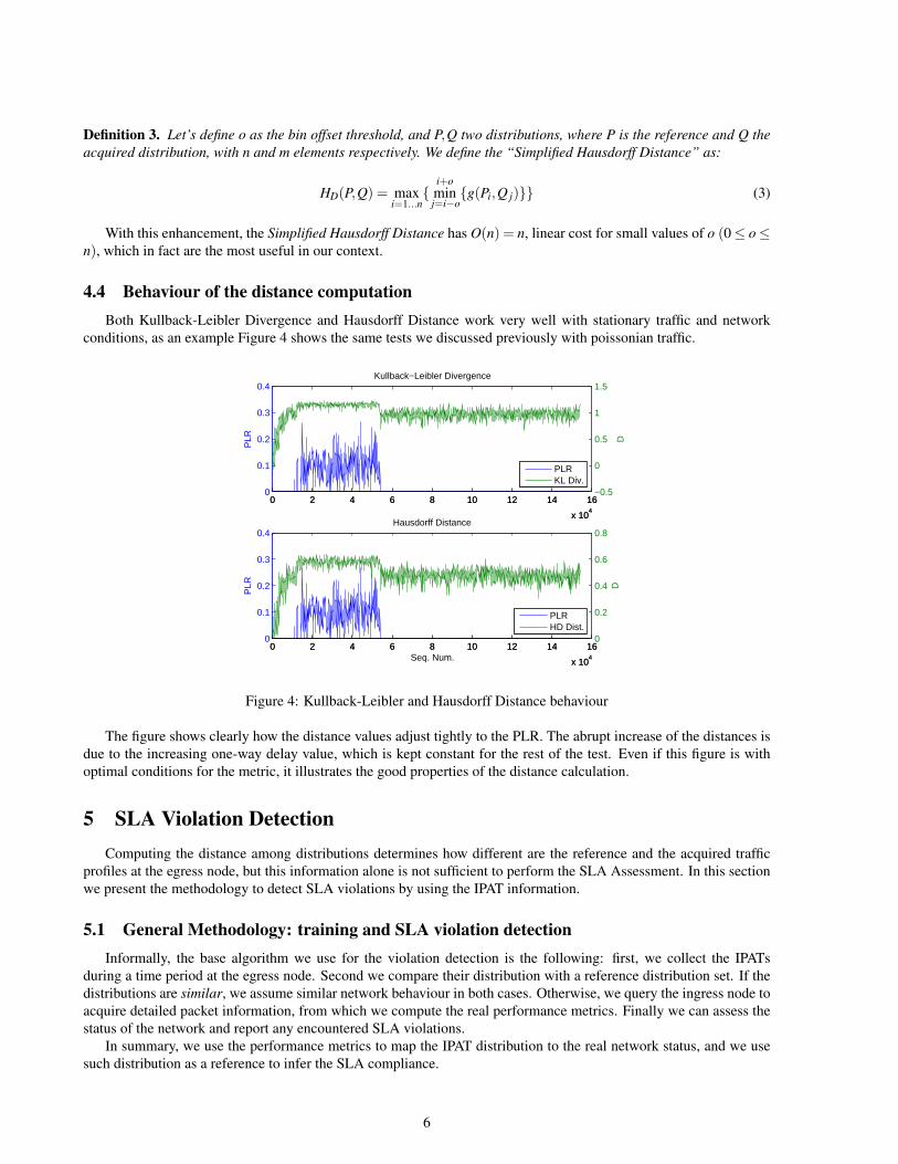
4.4 Behaviour of the distance computationBoth Kullback-Leibler Divergence and Hausdorff Distance work very well with stationary traffic and network

conditions, as an example Figure 4 shows the same tests we discussed previously with poissonian traffic.

0 2 4 6 8 10 12 14 16

x 104

0

0.1

0.2

0.3

0.4Kullback−Leibler Divergence

PLR

0 2 4 6 8 10 12 14 16

x 104

−0.5

0

0.5

1

1.5

D

0 2 4 6 8 10 12 14 16

x 104

0

0.1

0.2

0.3

0.4Hausdorff Distance

PLR

Seq. Num.

0 2 4 6 8 10 12 14 16

x 104

0

0.2

0.4

0.6

0.8

D

PLRKL Div.

PLRHD Dist.

Figure 4: Kullback-Leibler and Hausdorff Distance behaviour

The figure shows clearly how the distance values adjust tightly to the PLR. The abrupt increase of the distances isdue to the increasing one-way delay value, which is kept constant for the rest of the test. Even if this figure is withoptimal conditions for the metric, it illustrates the good properties of the distance calculation.

5 SLA Violation DetectionComputing the distance among distributions determines how different are the reference and the acquired traffic

profiles at the egress node, but this information alone is not sufficient to perform the SLA Assessment. In this sectionwe present the methodology to detect SLA violations by using the IPAT information.

5.1 General Methodology: training and SLA violation detectionInformally, the base algorithm we use for the violation detection is the following: first, we collect the IPATs

during a time period at the egress node. Second we compare their distribution with a reference distribution set. If thedistributions are similar, we assume similar network behaviour in both cases. Otherwise, we query the ingress node toacquire detailed packet information, from which we compute the real performance metrics. Finally we can assess thestatus of the network and report any encountered SLA violations.

In summary, we use the performance metrics to map the IPAT distribution to the real network status, and we usesuch distribution as a reference to infer the SLA compliance.

6

Algorithm 1 SLA AssessmentInput: f , D { f : Current Flow, D : Global RDS}S← getFlowSourceMP( f ) {Source Monitoring Point}Q← acquireDistribution( f )if D = ∅ then

5: status← Training(Q,S) {Does metric computation}else

status← compareDistributions(Q,S)end ifif status < ν then {Not valid network conditions}

10: trigger SLAViolation(status)end ifOutput: status

Algorithm 1 shows the general logic to perform the detection of SLA violation, regarding the collection of IPATdistributions, it is performed in a per flow f basis, during a predefined time interval t. The empirical distribution iscomputed in bins of width w (referring to IPAT ranges), therefore, a particular IPAT i falls in bin k = b i

wc. We deferthe study of proper t and w values to Section 9.

As a simple example, Figure 5 illustrates this behaviour, we assume a single flow and a single time interval.

P

1

P

2

P

3

P

4

P

5

P

6

P

7

P

8

P

9

t

Figure 5: Flow to distribution process

After the distribution acquisition, to cope with the aforementioned IPAT variability, our algorithm considers thefollowing actions:

• Training and update the traffic profile.

– Map it to the actual network status.– Update the set of valid distributions if needed.

• Compare the current profile with the learned status.

– Decide whether the traffic conditions changed or not.

The rest of the section performs a step by step description for the algorithm. We start by how the system learns thereal offered network quality. Later we focus in the distributions comparison.

5.2 Training and Update StrategyAny system with adaptability requirements must have a robust Training mechanism. Before entering with the full

description of the Training and Update Strategy, we need to define a few concepts.

Definition 4. A Valid IPAT Distribution (VID) V is such a distribution where a function of the real metrics (OWD,IPDV and PLR) fall above a specified SLA threshold ν. The complete discussion about how V is computed is done inSection 5.4.

Definition 5. Let’s define a Reference Distribution Set (RDS) D , as a set of strictly different VID distributions. Where|D| is the cardinality of the set, D1 is the first element and D |D| the last one, with a maximum size for the RDS boundedby a predefined ∆, which limits the maximum memory usage of the RDS.

7

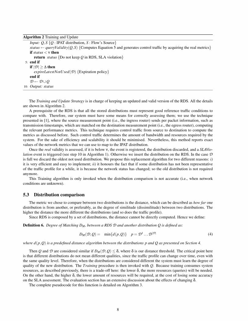
Algorithm 2 Training and UpdateInput: Q,S {Q : IPAT distribution, S : Flow’s Source}status← queryValidity(Q,S) {Computes Equation 5 and generates control traffic by acquiring the real metrics}if status < ν then

return status {Do not keep Q in RDS, SLA violation}5: end if

if |D| ≥ ∆ thenexpireLatestNotUsed(D) {Expiration policy}

end ifD←D ∪Q

10: Output: status

The Training and Update Strategy is in charge of keeping an updated and valid version of the RDS. All the detailsare shown in Algorithm 2.

A prerequisite of the RDS is that all the stored distributions must represent good reference traffic conditions tocompare with. Therefore, our system must have some means for correctly assessing them; we use the techniquepresented in [1], where the source measurement point (i.e., the ingress router) sends per packet information, such astransmission timestamps, which are matched on the destination measurement point (i.e., the egress router), computingthe relevant performance metrics. This technique requires control traffic from source to destination to compute themetrics as discussed before. Such control traffic determines the amount of bandwidth and resources required by thesystem. For the sake of efficiency and scalability it should be minimised. Nevertheless, this method reports exactvalues of the network metrics that we can use to map to the IPAT distribution.

Once the real validity is assessed, if it is below ν, the event is registered, the distribution discarded, and a SLAVio-lation event is triggered (see step 10 in Algorithm 1). Otherwise we insert the distribution on the RDS. In the case Dis full we discard the oldest not used distribution. We propose this replacement algorithm for two different reasons: i)it is very efficient and easy to implement; ii) it honours the fact that if some distribution has not been representativeof the traffic profile for a while, it is because the network status has changed; so the old distribution is not requiredanymore.

This Training algorithm is only invoked when the distribution comparison is not accurate (i.e., when networkconditions are unknown).

5.3 Distribution comparisonThe metric we chose to compare between two distributions is the distance, which can be described as how far one

distribution is from another, or preferably, as the degree of similitude (dissimilitude) between two distributions. Thehigher the distance the more different the distributions (and so does the traffic profile).

Since RDS is composed by a set of distributions, the distance cannot be directly computed. Hence we define:

Definition 6. Degree of Matching DM , between a RDS D and another distribution Q is defined as:

DM(D,Q) = min{d(p,Q)} p = D1 . . .D |D| (4)

where d(p,Q) is a predefined distance algorithm between the distributions p and Q as presented on Section 4.

Then Q and D are considered similar if DM(D,Q)≤ δ, where δ is our distance threshold. The critical point hereis that different distributions do not mean different qualities, since the traffic profile can change over time, even withthe same quality level. Therefore, when the distributions are considered different the system must learn the degree ofquality of the new distribution. The Training procedure is then invoked with Q. Because training consumes systemresources, as described previously, there is a trade-off here: the lower δ, the more resources (queries) will be needed.On the other hand, the higher δ, the lower amount of resources will be required, at the cost of losing some accuracyon the SLA assessment. The evaluation section has an extensive discussion about the effects of changing δ.

The complete pseudocode for this function is detailed on Algorithm 3.

8

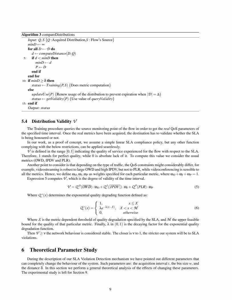
Algorithm 3 compareDistributionsInput: Q,S {Q :Acquired Distribution,S : Flow’s Source}minD← ∞

for all D←D dod← computeDistance(D,Q)

5: if d < minD thenminD← dP← D

end ifend for

10: if minD≥ δ thenstatus← Training(P,S) {Does metric computation}

elseupdateUse(P) {Renew usage of the distribution to prevent expiration when |D|= ∆}status← getValidity(P) {Use value of queryValidity}

15: end ifOutput: status

5.4 Distribution Validity VThe Training procedure queries the source monitoring point of the flow in order to get the real QoS parameters of

the specified time interval. Once the real metrics have been acquired, the destination has to validate whether the SLAis being honoured or not.

In our work, as a proof of concept, we assume a simple linear SLA compliance policy, but any other functioncomplying with the below restrictions, can be applied seamlessly.

V is defined in the range [0,1] indicating the quality of service experienced for the flow with respect to the SLA.Therefore, 1 stands for perfect quality, while 0 is absolute lack of it. To compute this value we consider the usualmetrics (OWD, IPDV and PLR).

Another point to consider is that depending on the type of traffic, the QoS constraints might considerably differ, forexample, videostreaming is robust to large OWD and high IPDV, but not to PLR, while videoconferencing is sensible toall the metrics. Hence, we define ωO,ωI ,ωP as weights specified for each particular metric, where ωO +ωI +ωP = 1.

Expression 5 computes V , which is the degree of validity of the time interval.

V = Q O(OWD) ·ωO +Q I(|IPDV |) ·ωI +Q P(PLR) ·ωP (5)

Where Q ∗(x) determines the exponential quality degrading function defined as:

Q ∗(x) =

1, x≤ Xλe−λ(x−X ), X < x < M0, otherwise

(6)

Where X is the metric dependent threshold of quality degradation specified by the SLA, and M the upper feasiblebound for the quality of that particular metric. Finally, λ in (0,1) is the decaying factor for the exponential qualitydegradation function.

Then V ≥ ν the network behaviour is considered stable. The closer is ν to 1, the stricter our system will be to SLAviolations.

6 Theoretical Parameter StudyDuring the description of our SLA Violation Detection mechanism we have pointed out different parameters that

can completely change the behaviour of the system. Such parameters are: the acquisition interval t, the bin size w, andthe distance δ. In this section we perform a general theoretical analysis of the effects of changing these parameters.The experimental study is left for Section 9.

9

6.1 The acquisition interval t

The acquisition interval is the first critical parameter we have to study to tune our SLA violation detection system.Tweaking such parameter has a number of implications depending on its size.

Here we detail separately the different effects caused by increasing and decreasing t.

Increasing t

Increasing the acquisition time interval has the following positive effects:

• More samples to consider: This implies that we will have more statistical soundness as the number of samplesincreases. Hence, our distributions are more statistically representative of the real network status.

• Better Training periods: If the acquired traffic is suitable to be part of the RDS then its distribution will be moreindicative since it considers larger time periods. From the practical point of view this implies that the referencedistributions will be more valid.

On the other hand, having large sizes of t derives in a number of negative effects:

• Increased lag on the reporting: The most important implication is that t determines the degree of “Reactivity” ofthe system, (i.e., the response time of the reporting). To understand this point, we have to have a clear idea aboutthe system behaviour in general. First we gather IPAT during t time units, after this we compare its distributionwith the RDS, and if necessary, we ask the ingress point about particular network metrics. The ingress pointresponds back with per packet information.

As it can be noted, one of the critical parameters for this response time, is the time t itself, which bounds thetime required to compute the distances, and therefore, start the violation detection process.

Other factors such as the time invested by the comparison algorithm, or the network latency, are also relevantbut out of the scope of this particular study.

• More probability of varying traffic: The longer we get statistics the more probable is that we have variations onthe underlying network, which on its turn makes it more difficult to have representative distributions.

Decreasing t

Reducing the acquisition time t also has positive and negative effects over the system behaviour. The positiveimplication are:

• More interactivity on the reporting: the less time we spend on the gathering the quicker we will react to anySLA violation.

• Less samples: Having less samples implies that we will have faster computation, hence, faster reporting.

Nevertheless, it also has a number of negative effects:

• Less samples: At the same time of being a good thing, having less samples means that we will have lessstatistical information in our distribution, therefore, we could incurr in inaccuracies in the detection.

• More variability: Derived from the previous case, the less samples we have, the higher is the probability ofhaving different distributions. Therefore, we will have more queries to the ingress node (even if these queriesare faster and smaller because of the reduced number of samples per time interval). This does not necessarilymeans that it will require more resources. In fact, as we show in below sections decreasing t usually impliesalso a reduction in resource requirements.

10

6.2 The bin size w

As we discussed previously, one of the most critical parameters of our SLA violation detection system is the binsize w.

Intuitively, w determines the degree of granularity of our system. Hence, for little values of w, we will have highresolution, which means that we distiguish among closer values per bin. On the other hand, if we increase the bin size,we are losing resolution, that is, we are aggregating a larger set of IPAT within the same bin. This, as expected, has anumber of effects over the final result. In this section we perform a basic theoretical study about the effects of tuningthe bin size. We defer the experimental analysis to section 9.2.

Increasing w

As introduced before, increasing w reduces our resolution in terms of higher aggregation degrees in our bins. Whenwe have larger w, we can observe different effects. The good properties of having large w are:

• Less bins to analyse: Since our aggregation level is higher, for a given tests we are reducing the number of binsto consider per t interval.

• More efficient: Derived from the previous advantage, having less bins implies less processing time to calculatethe IPAT, generate the distributions, and perform the distance comparisons.

• Less network resources: Reducing the amount of bins implies that we will have less probability of havingdifferent distributions. We can formally prove this:

Proof. Let’s define p as a reference distribution, and Q as the acquired distribution. Assuming that w→ ∞ forthe acquisition interval then the probability P of having exact IPAT distributions is determined by:

limw→∞

DM(p,Q) = 0 (7)

Therefore, P(DM(p,Q) ≤ δ) = 1 for any p, Q, and δ. Hence, the system will consider all the distributions asequal.

On the other hand, if w→ 0 we have infinite bins, by basic statistics we know that P(DM(p,Q)≤ δ)→ 0 sincewe have more bins to match, therefore having two exact distributions is much less probable.

The final effect then is that we invoke the Training process fewer times, hence, reducing the required networkresources. But this reduction of the resources is not for free, it has some bad implications as we detail now:

• Less accuracy: Analogously to the fact that we have higher probability of having similar distributions, we willconsider different traffic profiles as equal with higher accuracy, which in practice means that we will reduce thedetection of SLA violations, mostly due to lack of Training.

Decreasing w

In the case that we are reducing the bin size, we will face opposite effects than before. In particular, the positiveeffects of decreasing w are:

• Finer accuracy: The more bins we have to compare, the more resolution we have in order to distinguish differentIPAT distributions. This leads to the fact that in general we have more accuracy in the reporting.

But, as expected, this also leads to some negative properties:

• More computation time: Derived from above, if we have more bins to analyse, it implies that we will need moretime to compute the IPATs distributions so we need more CPU power to do the on-line detection.

• More network resources: If we have finer detail in the IPAT distribution as detailed above the probability ofequal distributions decreases, meaning that we invoke the Training process more often, which leads to highernetwork resource requirements.

As it can be noted there is a trade-off in this situation, normally we desire good accuracy, but in practice thenetwork resources reserved for control traffic are limited. In Section 9.2 we experimentally show such effects.

11

6.3 The Distance threshold δ

The last system parameter to study is the distance threshold δ. It determines the confidence we have in ourdistance algorithm, high values represent loose constraints on the distance comparison, while small values indicatetight constraints that trigger the Training process more easily. Therefore, there is a trade-off selecting the size of thisparameter.

Increasing δ

Increasing δ implies that we are relaxing the constraints of our distace algorithms. In practice, this means that weconsider as similar very different distributions.

In detail, since the outcome of the distance algorithms range in [0..1], for values of δ closer to 1 the algorithmcannot distinguish among the distributions and all of them are considered as equal. This, as expected, comes with anassociated loss in accuracy.

The good side of this increase, is the considerable reduction in control traffic derived of such action. If we considertwo distributions as equan we do not need to invoke the Training, thus, we reduce the required resources.

Decreasing δ

Logically, decreasing δ, gives the opposite effect, this means that for δ→ 0 we are tightening the constraits of oursimilarity threshold, which make more difficult for our algorithm consider two different distributions as similar. Thisimples that we will increase the accuracy, toghether with an increase in the used network resources.

7 Tests and TestbedsIn order to validate our proposal we set up three different testbeds, where we performed several tests. In particular,

i) synthetic traffic under controlled testbed conditions, ii) synthetic traffic over the European Research network Geant,iii) real traffic over a controlled testbed.

7.1 Synthetic traffic under controlled testbed conditionsThe first set of tests have been performed under a tightly controlled environment. We configured two end nodes

with Linux Debian in order to generate and collect traffic. On the core of the testbed we installed two servers also withLinux Debian, Traffic Control and NetEM emulator capabilities. We then can change the network conditions accordingto our needs and experience a wide range of controlled network disruptions.

Figure 6: Controlled testbed

All the links on the testbed were configured with Fast Ethernet and no cross traffic. Furthermore, all the Linuxboxes were synchronised by using GPS signal with NTP and PPS patches on the kernel for accurate timestamping.

In this testbed the set of emulated network conditions are:

1. Good Network Conditions: no SLA disruptions and good network behaviour all over the test.

2. Mild Network Disruptions: moderated increase of OWD with periods of high IPDV and some packet losses.Some traffic disruptions but only with few SLA violations per test.

3. Medium Network Disruptions: similar to the mild network disruptions but with limited buffers on the routerswhich leads to moderate periods of packet losses. Some SLA violations in many intervals during the test.

12

4. Severe Network Disruptions: random losses from 1% to 10% with variable OWD. Severe SLA violations inperiodic intervals on the test.

All the tests have in common that the SLA disruptions are applied at regular time intervals all over the tests,combining periods of good behaviour with others with disruptions.

We performed tests with Periodic, Poissonian and Synthetic Real Traffic [16] traffic profiles with all the abovenetwork conditions. Since the controlled traffic conditions are tightly controlled, to have meaningful results it wasenough to repeat 3 times each set of tests. Using these traffic profiles we have from predictable packet rates (Periodic)to unpredictable realistic profiles (Synthetic Real Traffic).

7.2 Synthetic traffic over the European Research networkIn this testbed we performed a set of more than 500 experimental tests during 2006 and 2007 using twelve different

testbeds across Europe. We performed the tests at different hours, including weekends, to have a real variety of crosstraffic and congestion. The testbeds were provided by the IST-EuQoS [17] partners, covering a total of 5 countries and4 different access technologies (LAN, xDSL, UMTS and WiFi) with an overlay architecture over the Geant researchnetwork.

We evaluated the performance of our system by actively generating UDP traffic on the network with differentproperties. Specifically, we generated periodic flows, with varying packet rates, from 16 to 900 packets per secondamong all the involved nodes in the testbed. We used different packet sizes ranging from 80 to 1500 bytes per packet.Specifically, we focus on three different sets of tests. The first one simulates a low rate, small size packets with a usedbandwidth of 64Kbps. We label this traces as (synthetic) VoIP.

The second type of traffic is a periodic flow with average packet rate of ∼ 96 packets per second, with MTU sizepackets amounting to a total of 1Mbps of UDP traffic. We call this trace UDP1. Finally, the third kind of traffic is aaverage sized, high rate UDP flow with ∼ 1.4Mbps. We call this test UDP2.

7.3 Real traffic over a controlled testbedGenerating synthetic traffic gives tight control over the different characteristics of the traffic to stress: rate, packet

size, etc., but on the other hand, it does not reflect how a real application performs. Therefore, in order to have insightsabout the behaviour of our system with real applications we used the local testbed described before in Section 7.1 witha video streaming application, namely VLC, transmitting high quality video with variable bit rate over the network.In the same fashion as before, we inserted various degrees of network disruption to analyse the accuracy of our SLAassessment system.

8 EvaluationThe validation of the proposal is issued by performing a wide variety of tests in different testbeds as described on

the previous section.We focus the study in the system’s accuracy, that is, in the SLA violation detection rate, measured in terms of false

negatives (i.e., not detected SLA violations). We compare the three presented distance algorithms against the case ofhaving perfect knowledge about the SLA violations. We also analyse the amount of resources required by the system;such resources are counted in terms of reduction ratio of the required bandwith used by the control traffic. Therefore,we compare the cost of reporting per packet information with our solution, which only demands information whenthere is a change in the traffic reception profile.

During all the analysis we use the same parameters across the tests for the estimation. In particular, we set up, asa proof of concept, the following values: distance threshold of δ = 3%, bin width of w = 3ms, and an acquisition timeinterval of t = 175ms. The discussion about the different parameters, such as distance threshold selection, or time binsize is done in Section 9.

8.1 MethodologyAnalysing all the information obtained from the tests is complex. To ease the comprehension of the validation

process, we unify the evaluation for all the tests and testbeds under the same methodology as follows:

13

1. For each test we collect the full trace on both end nodes.

2. We match the packets extracting the network performance metrics as described in [1], using them as referencequality (perfect knowledge), since the process gives exact results.

3. We identify the different SLA violation periods with the reference results acquired above.

4. We apply off-line our algorithm (by using Kullback-Leibler, Hausdorff and Simplified Hausdorff ). Here weregister: i) required control traffic due to Training. ii) estimated SLA violation periods.

5. Finally, we match the SLA violations with the ones obtained in Step 3.

We apply our system off-line with the goal of comparing the results. But in the actual deployment the systemperforms on-line assessment. By using this methodology we can guarantee accurate comparison between the perfectknowledge of the network behaviour and our system.

8.2 Accuracy and Resources requirementsIn order to study the behaviour of our system, here we discuss the achieved accuracy together with the analysis of

the required resources for each algorithm in the different testbeds.

8.2.1 Synthetic traffic with controlled network

The goal of this synthetic traffic generation is to evaluate the reaction of each algorithm in a controlled environmentwith the different traffic profiles.

We analyse in Table 1 the Accuracy and the Resource utilisation for the different generated traffic. The accuracy iscomputed for the overall test duration, counting the ratio of detected SLA violations over the total, while the requiredresources are computed by the ratio of the actual number of queries, over the maximum possible queries per test. Ourgoal is to achieve high accuracy with low resource consumption.

(a) Periodic

AccuracyGood Mild Medium Severe

KL 1.000 1.000 0.987 1.000Hausdorff 1.000 1.000 0.088 1.000

D. Haus. 1.000 1.000 0.868 1.000Resources

Good Mild Medium SevereKL 0.001 0.256 0.385 0.394

Hausdorff 0.001 0.020 0.019 0.394D. Haus. 0.001 0.130 0.267 0.394

(b) Poisson


KL 1.000 0.250 0.940 0.893Hausdorff 1.000 0.750 0.067 0.225

D. Haus. 1.000 1.000 0.994 0.999Resources


Hausdorff 0.122 0.143 0.132 0.190D. Haus. 0.464 0.601 0.699 0.721

(c) Synthetic Real Traffic


KL 1.000 0.667 1.000 1.000Hausdorff 1.000 1.000 1.000 1.000

D. Haus. 1.000 0.667 1.000 1.000Resources


Hausdorff 0.002 0.003 0.397 0.397D. Haus. 0.002 0.002 0.397 0.397

Table 1: Accuracy and Resources for δ = 0.03

14

As it can be observed in the table, the accuracy of the solution is higher for the extreme cases. When there areGood network conditions in the network we always estimate correctly, and with very low resource consumption ingeneral. This is because our algorithm assumes correct network behaviour by design. In the case of Severe networkconditions, where our contribution is more useful, we can detect with very good accuracy the SLA disruption periods.On the other hand, in the fuzzy case when there are few SLA violations, the accuracy of the system drops sensiblyfor some algorithms. The cause of this is the statistical resolution achieved when there are few SLA violations, wheremissing only one violation is statistically significative. Moreover, in a real deployment, such SLA violations are ofno practical interest since they represent very short, sporadic, periods of light congestion, with no high impact on thefinal network behaviour.

Comparing the various distance algorithms we can notice some general properties: first, the better accuracy in mostcases is achieved by the Simplified Hausdorff Distance proposed as an extension in this paper, with similar results forKullback-Leibler. It is also interesting to highlight the poor performance obtained with Hausdorff, except in the caseof synthetic real traffic. This is caused by the “all-against-all” comparison we pointed out previously.

The second consideration is the resources needed by the Severe, and some Medium network conditions. As it canbe noted, in some traffic profiles, the results are exactly the same regardless of the algorithm used. This is because thealgorithms always query the ingress node when an unknown IPAT distribution is found. With bad network conditionsthis situation is common. Hence it forces the system to query for exact metrics. Here the minimum number of queriesis bounded by the amount of SLA violations, which in our experimental case is 0.39 as shown in the Table 1. In thespecific case of Poissonian Traffic, we need more resources than this lower bound for Kullback-Leibler and SimplifiedHausdorff. Notice though, that requiring less resources than that implies non detection of some SLA violations.

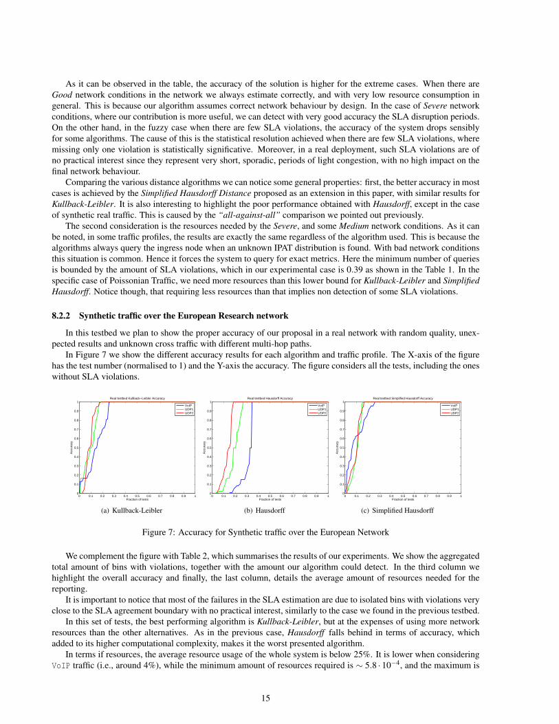
8.2.2 Synthetic traffic over the European Research network

In this testbed we plan to show the proper accuracy of our proposal in a real network with random quality, unex-pected results and unknown cross traffic with different multi-hop paths.

In Figure 7 we show the different accuracy results for each algorithm and traffic profile. The X-axis of the figurehas the test number (normalised to 1) and the Y-axis the accuracy. The figure considers all the tests, including the oneswithout SLA violations.

0 0.1 0.2 0.3 0.4 0.5 0.6 0.7 0.8 0.9 10

0.1

0.2

0.3

0.4

0.5

0.6

0.7

0.8

0.9

1

Fraction of tests

Acc

urac

y

Real testbed Kullback−Leibler Accuracy

VoIPUDP1UDP2

(a) Kullback-Leibler

0 0.1 0.2 0.3 0.4 0.5 0.6 0.7 0.8 0.9 10

0.1

0.2

0.3

0.4

0.5

0.6

0.7

0.8

0.9

1

Fraction of tests

Acc

urac

y

Real testbed Hausdorff Accuracy

VoIPUDP1UDP2

(b) Hausdorff

0 0.1 0.2 0.3 0.4 0.5 0.6 0.7 0.8 0.9 10

0.1

0.2

0.3

0.4

0.5

0.6

0.7

0.8

0.9

1

Fraction of tests

Acc

urac

y

Real testbed Simplified Hausdorff Accuracy

VoIPUDP1UDP2

(c) Simplified Hausdorff

Figure 7: Accuracy for Synthetic traffic over the European Network

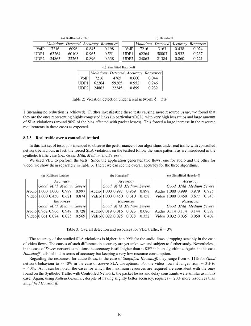
We complement the figure with Table 2, which summarises the results of our experiments. We show the aggregatedtotal amount of bins with violations, together with the amount our algorithm could detect. In the third column wehighlight the overall accuracy and finally, the last column, details the average amount of resources needed for thereporting.

It is important to notice that most of the failures in the SLA estimation are due to isolated bins with violations veryclose to the SLA agreement boundary with no practical interest, similarly to the case we found in the previous testbed.

In this set of tests, the best performing algorithm is Kullback-Leibler, but at the expenses of using more networkresources than the other alternatives. As in the previous case, Hausdorff falls behind in terms of accuracy, whichadded to its higher computational complexity, makes it the worst presented algorithm.

In terms if resources, the average resource usage of the whole system is below 25%. It is lower when consideringVoIP traffic (i.e., around 4%), while the minimum amount of resources required is ∼ 5.8 ·10−4, and the maximum is

15


Violations Detected Accuracy ResourcesVoIP 7216 6096 0.845 0.198

UDP1 62264 60108 0.965 0.551UDP2 24863 22265 0.896 0.338

(b) Hausdorff


UDP1 62264 58003 0.932 0.237UDP2 24863 21384 0.860 0.221



UDP1 62264 59265 0.952 0.246UDP2 24863 22345 0.899 0.232

Table 2: Violation detection under a real network, δ = 3%

1 (meaning no reduction is achieved). Further investigating these tests causing more resource usage, we found thatthey are the ones representing highly congested links (in particular xDSL), with very high loss ratios and large amountof SLA violations (around 90% of the bins affected with packet losses). This forced a large increase in the resourcerequirements in these cases as expected.

8.2.3 Real traffic over a controlled testbed

In this last set of tests, it is intended to observe the performance of our algorithms under real traffic with controllednetwork behaviour, in fact, the forced SLA violations on the testbed follow the same patterns as we introduced in thesynthetic traffic case (i.e., Good, Mild, Medium and Severe).

We used VLC to perform the tests. Since the application generates two flows, one for audio and the other forvideo, we show them separately in Table 3. There, we can see the overall accuracy for the three algorithms.



Audio 1.000 1.000 0.999 0.997Video 1.000 0.450 0.621 0.874

ResourcesGood Mild Medium Severe

Audio 0.962 0.966 0.947 0.728Video 0.061 0.074 0.085 0.569

(b) Hausdorff


Audio 1.000 0.997 0.969 0.898Video 1.000 0.450 0.610 0.758


Audio 0.019 0.016 0.023 0.086Video 0.022 0.025 0.038 0.352



Audio 1.000 0.999 0.979 0.975Video 1.000 0.450 0.677 0.848


Audio 0.114 0.114 0.144 0.397Video 0.032 0.035 0.050 0.407

Table 3: Overall detection and resources for VLC traffic, δ = 3%

The accuracy of the studied SLA violations is higher than 99% for the audio flows, dropping sensibly in the caseof video flows. The causes of such difference in accuracy are yet unknown and subject to further study. Nevertheless,in the case of Severe network conditions the accuracy is still higher than∼ 85% in both algorithms. Again, in this caseHausdorff falls behind in terms of accuracy but keeping a very low resource consumption.

Regarding the resources, for audio flows, in the case of Simplified Hausdorff, they range from ∼ 11% for Goodnetwork behaviour to ∼ 40% in the case of Severe SLA disruptions. For the video flows it ranges from ∼ 3% to∼ 40%. As it can be noted, the cases for which the maximum resources are required are consistent with the onesfound on the Synthetic Traffic with Controlled Network: the packet losses and delay constraints were similar as in thiscase. Again, using Kullback-Leibler, despite of having slightly better accuracy, requires ∼ 20% more resources thanSimplified Hausdorff.

16

9 Experimental Parameter tuningComplementary to the theoretical analysis performed in Section 6, this section studies all the different experimental

parameter selection and tunning for our system. Specifically, the considered parameters are: the acquisition interval t,the bin size w, and the distance δ.

All the parameters are studied by using the tests described above, in particular for the study of t and w we use RealTraffic over a Controlled Network, with the VLC flows. Regarding the δ we use the Poissonian flows generated underthe EuQoS project.

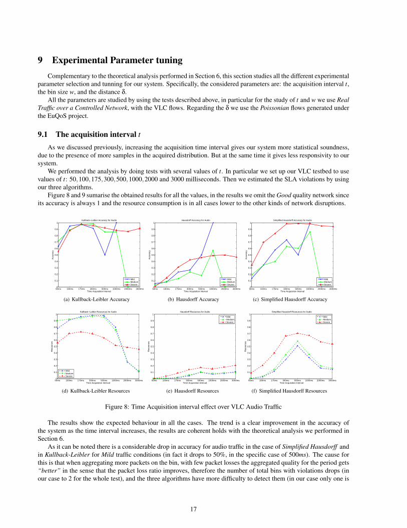
9.1 The acquisition interval t

As we discussed previously, increasing the acquisition time interval gives our system more statistical soundness,due to the presence of more samples in the acquired distribution. But at the same time it gives less responsivity to oursystem.

We performed the analysis by doing tests with several values of t. In particular we set up our VLC testbed to usevalues of t: 50,100,175,300,500,1000,2000 and 3000 milliseconds. Then we estimated the SLA violations by usingour three algorithms.

Figure 8 and 9 sumarise the obtained results for all the values, in the results we omit the Good quality network sinceits accuracy is always 1 and the resource consumption is in all cases lower to the other kinds of network disruptions.

50ms 100ms 175ms 300ms 500ms 1000ms 2000ms 3000ms0

0.1

0.2

0.3

0.4

0.5

0.6

0.7

0.8

0.9

1

Time Acquisition Interval

Acc

urac

y

Kullback−Leibler Accuracy for Audio

MildMediumSevere

(a) Kullback-Leibler Accuracy


0.1

0.2

0.3

0.4

0.5

0.6

0.7

0.8

0.9

1


Acc

urac

y

Hausdorff Accuracy for Audio

MildMediumSevere

(b) Hausdorff Accuracy


0.1

0.2

0.3

0.4

0.5

0.6

0.7

0.8

0.9

1


Acc

urac

y

Simplified Hausdorff Accuracy for Audio

MildMediumSevere

(c) Simplified Hausdorff Accuracy


0.1

0.2

0.3

0.4

0.5

0.6

0.7

0.8

0.9

1


Res

ourc

es

Kullback−Leibler Resources for Audio

MildMediumSevere

(d) Kullback-Leibler Resources


0.1

0.2

0.3

0.4

0.5

0.6

0.7

0.8

0.9

1


Res

ourc

es

Hausdorff Resources for Audio

MildMediumSevere

(e) Hausdorff Resources


0.1

0.2

0.3

0.4

0.5

0.6

0.7

0.8

0.9

1


Res

ourc

es

Simplified Hausdorff Resources for Audio

MildMediumSevere

(f) Simplified Hausdorff Resources

Figure 8: Time Acquisition interval effect over VLC Audio Traffic

The results show the expected behaviour in all the cases. The trend is a clear improvement in the accuracy ofthe system as the time interval increases, the results are coherent holds with the theoretical analysis we performed inSection 6.

As it can be noted there is a considerable drop in accuracy for audio traffic in the case of Simplified Hausdorff andin Kullback-Leibler for Mild traffic conditions (in fact it drops to 50%, in the specific case of 500ms). The cause forthis is that when aggregating more packets on the bin, with few packet losses the aggregated quality for the period gets“better” in the sense that the packet loss ratio improves, therefore the number of total bins with violations drops (inour case to 2 for the whole test), and the three algorithms have more difficulty to detect them (in our case only one is

17


0.1

0.2

0.3

0.4

0.5

0.6

0.7

0.8

0.9

1


Acc

urac

y

Kullback−Leibler Accuracy for Video

MildMediumSevere



0.1

0.2

0.3

0.4

0.5

0.6

0.7

0.8

0.9

1


Acc

urac

y

Hausdorff Accuracy for Video

MildMediumSevere



0.1

0.2

0.3

0.4

0.5

0.6

0.7

0.8

0.9

1


Acc

urac

y

Simplified Hausdorff Accuracy for Video

MildMediumSevere



0.1

0.2

0.3

0.4

0.5

0.6

0.7

0.8

0.9

1


Res

ourc

es

Kullback−Leibler Resources for Video

MildMediumSevere



0.1

0.2

0.3

0.4

0.5

0.6

0.7

0.8

0.9

1


Res

ourc

es

Hausdorff Resources for Video

MildMediumSevere



0.1

0.2

0.3

0.4

0.5

0.6

0.7

0.8

0.9

1


Res

ourc

es

Simplified Hausdorff Resources for Video

MildMediumSevere


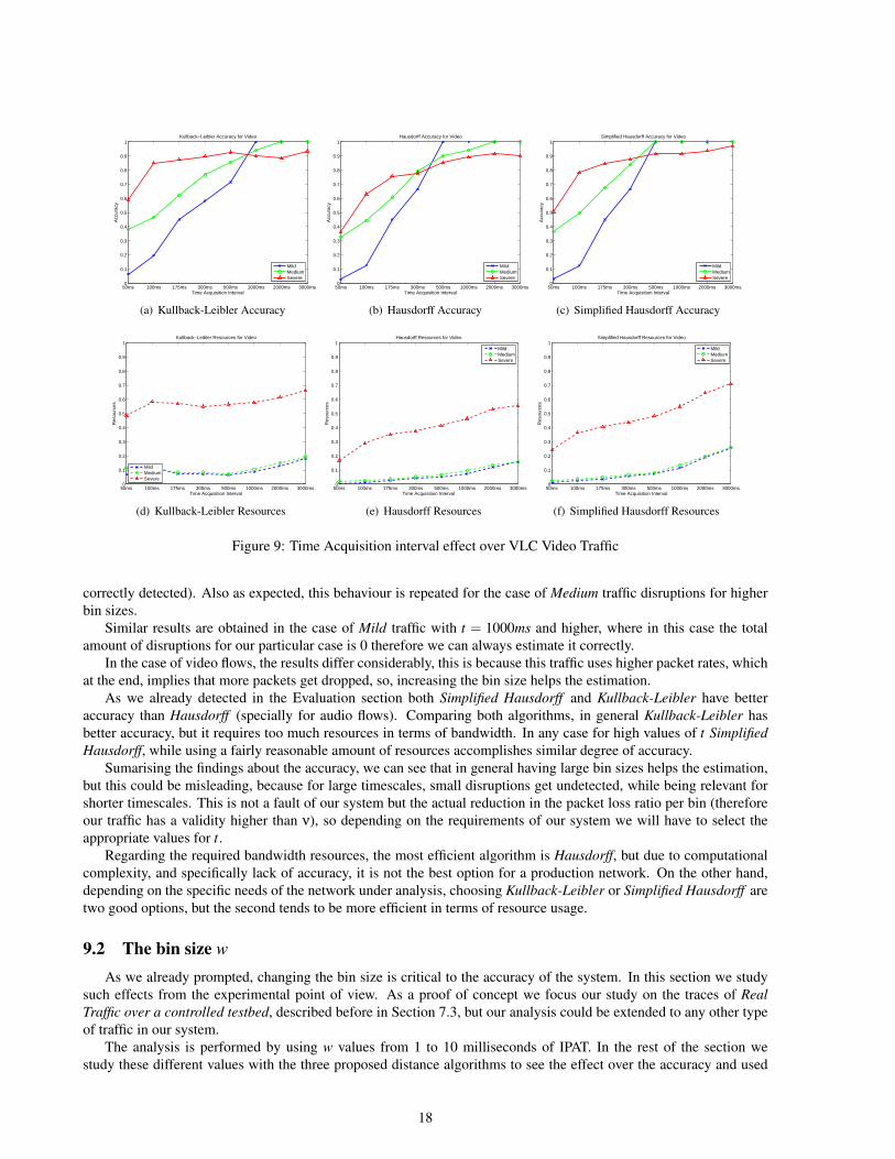
Figure 9: Time Acquisition interval effect over VLC Video Traffic

correctly detected). Also as expected, this behaviour is repeated for the case of Medium traffic disruptions for higherbin sizes.

Similar results are obtained in the case of Mild traffic with t = 1000ms and higher, where in this case the totalamount of disruptions for our particular case is 0 therefore we can always estimate it correctly.

In the case of video flows, the results differ considerably, this is because this traffic uses higher packet rates, whichat the end, implies that more packets get dropped, so, increasing the bin size helps the estimation.

As we already detected in the Evaluation section both Simplified Hausdorff and Kullback-Leibler have betteraccuracy than Hausdorff (specially for audio flows). Comparing both algorithms, in general Kullback-Leibler hasbetter accuracy, but it requires too much resources in terms of bandwidth. In any case for high values of t SimplifiedHausdorff, while using a fairly reasonable amount of resources accomplishes similar degree of accuracy.

Sumarising the findings about the accuracy, we can see that in general having large bin sizes helps the estimation,but this could be misleading, because for large timescales, small disruptions get undetected, while being relevant forshorter timescales. This is not a fault of our system but the actual reduction in the packet loss ratio per bin (thereforeour traffic has a validity higher than ν), so depending on the requirements of our system we will have to select theappropriate values for t.

Regarding the required bandwidth resources, the most efficient algorithm is Hausdorff, but due to computationalcomplexity, and specifically lack of accuracy, it is not the best option for a production network. On the other hand,depending on the specific needs of the network under analysis, choosing Kullback-Leibler or Simplified Hausdorff aretwo good options, but the second tends to be more efficient in terms of resource usage.

9.2 The bin size w

As we already prompted, changing the bin size is critical to the accuracy of the system. In this section we studysuch effects from the experimental point of view. As a proof of concept we focus our study on the traces of RealTraffic over a controlled testbed, described before in Section 7.3, but our analysis could be extended to any other typeof traffic in our system.

The analysis is performed by using w values from 1 to 10 milliseconds of IPAT. In the rest of the section westudy these different values with the three proposed distance algorithms to see the effect over the accuracy and used

18

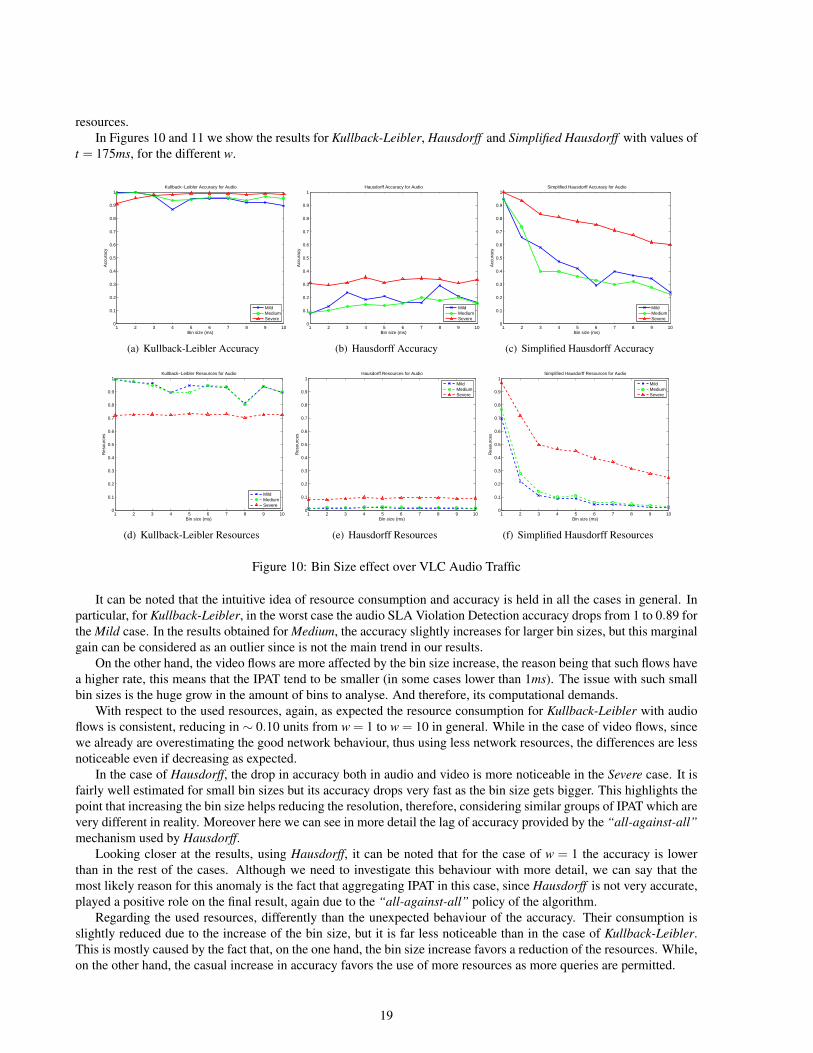
resources.In Figures 10 and 11 we show the results for Kullback-Leibler, Hausdorff and Simplified Hausdorff with values of

t = 175ms, for the different w.

1 2 3 4 5 6 7 8 9 100

0.1

0.2

0.3

0.4

0.5

0.6

0.7

0.8

0.9

1

Bin size (ms)

Acc

urac

y

Kullback−Leibler Accuracy for Audio

MildMediumSevere


1 2 3 4 5 6 7 8 9 100

0.1

0.2

0.3

0.4

0.5

0.6

0.7

0.8

0.9

1

Bin size (ms)

Acc

urac

y

Hausdorff Accuracy for Audio

MildMediumSevere


1 2 3 4 5 6 7 8 9 100

0.1

0.2

0.3

0.4

0.5

0.6

0.7

0.8

0.9

1

Bin size (ms)

Acc

urac

y

Simplified Hausdorff Accuracy for Audio

MildMediumSevere


1 2 3 4 5 6 7 8 9 100

0.1

0.2

0.3

0.4

0.5

0.6

0.7

0.8

0.9

1

Bin size (ms)

Res

ourc

es

Kullback−Leibler Resources for Audio

MildMediumSevere


1 2 3 4 5 6 7 8 9 100

0.1

0.2

0.3

0.4

0.5

0.6

0.7

0.8

0.9

1

Bin size (ms)

Res

ourc

es

Hausdorff Resources for Audio

MildMediumSevere


1 2 3 4 5 6 7 8 9 100

0.1

0.2

0.3

0.4

0.5

0.6

0.7

0.8

0.9

1

Bin size (ms)

Res

ourc

es

Simplified Hausdorff Resources for Audio

MildMediumSevere


Figure 10: Bin Size effect over VLC Audio Traffic

It can be noted that the intuitive idea of resource consumption and accuracy is held in all the cases in general. Inparticular, for Kullback-Leibler, in the worst case the audio SLA Violation Detection accuracy drops from 1 to 0.89 forthe Mild case. In the results obtained for Medium, the accuracy slightly increases for larger bin sizes, but this marginalgain can be considered as an outlier since is not the main trend in our results.

On the other hand, the video flows are more affected by the bin size increase, the reason being that such flows havea higher rate, this means that the IPAT tend to be smaller (in some cases lower than 1ms). The issue with such smallbin sizes is the huge grow in the amount of bins to analyse. And therefore, its computational demands.

With respect to the used resources, again, as expected the resource consumption for Kullback-Leibler with audioflows is consistent, reducing in ∼ 0.10 units from w = 1 to w = 10 in general. While in the case of video flows, sincewe already are overestimating the good network behaviour, thus using less network resources, the differences are lessnoticeable even if decreasing as expected.

In the case of Hausdorff, the drop in accuracy both in audio and video is more noticeable in the Severe case. It isfairly well estimated for small bin sizes but its accuracy drops very fast as the bin size gets bigger. This highlights thepoint that increasing the bin size helps reducing the resolution, therefore, considering similar groups of IPAT which arevery different in reality. Moreover here we can see in more detail the lag of accuracy provided by the “all-against-all”mechanism used by Hausdorff.

Looking closer at the results, using Hausdorff, it can be noted that for the case of w = 1 the accuracy is lowerthan in the rest of the cases. Although we need to investigate this behaviour with more detail, we can say that themost likely reason for this anomaly is the fact that aggregating IPAT in this case, since Hausdorff is not very accurate,played a positive role on the final result, again due to the “all-against-all” policy of the algorithm.

Regarding the used resources, differently than the unexpected behaviour of the accuracy. Their consumption isslightly reduced due to the increase of the bin size, but it is far less noticeable than in the case of Kullback-Leibler.This is mostly caused by the fact that, on the one hand, the bin size increase favors a reduction of the resources. While,on the other hand, the casual increase in accuracy favors the use of more resources as more queries are permitted.

19

1 2 3 4 5 6 7 8 9 100

0.1

0.2

0.3

0.4

0.5

0.6

0.7

0.8

0.9

1

Bin size (ms)

Acc

urac

y

Kullback−Leibler Accuracy for Video

MildMediumSevere


1 2 3 4 5 6 7 8 9 100

0.1

0.2

0.3

0.4

0.5

0.6

0.7

0.8

0.9

1

Bin size (ms)

Acc

urac

y

Hausdorff Accuracy for Video

MildMediumSevere


1 2 3 4 5 6 7 8 9 100

0.1

0.2

0.3

0.4

0.5

0.6

0.7

0.8

0.9

1

Bin size (ms)

Acc

urac

y

Simplified Hausdorff Accuracy for Video

MildMediumSevere


1 2 3 4 5 6 7 8 9 100

0.1

0.2

0.3

0.4

0.5

0.6

0.7

0.8

0.9

1


Res

ourc

es

Kullback−Leibler Resources for Video

MildMediumSevere


1 2 3 4 5 6 7 8 9 100

0.1

0.2

0.3

0.4

0.5

0.6

0.7

0.8

0.9

1

Bin size (ms)

Res

ourc

es

Hausdorff Resources for Video

MildMediumSevere


1 2 3 4 5 6 7 8 9 100

0.1

0.2

0.3

0.4

0.5

0.6

0.7

0.8

0.9

1


Res

ourc

es

Simplified Hausdorff Resources for Video

MildMediumSevere


Figure 11: Bin Size effect over VLC Video Traffic

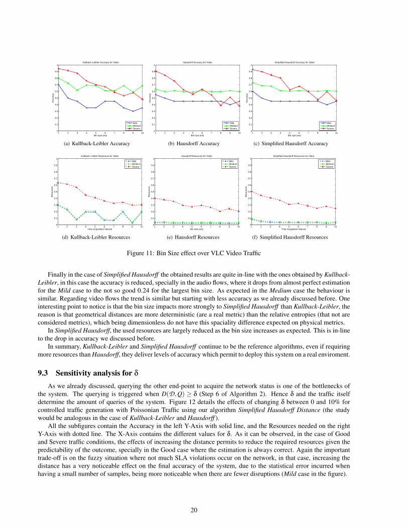
Finally in the case of Simplified Hausdorff the obtained results are quite in-line with the ones obtained by Kullback-Leibler, in this case the accuracy is reduced, specially in the audio flows, where it drops from almost perfect estimationfor the Mild case to the not so good 0.24 for the largest bin size. As expected in the Medium case the behaviour issimilar. Regarding video flows the trend is similar but starting with less accuracy as we already discussed before. Oneinteresting point to notice is that the bin size impacts more strongly to Simplified Hausdorff than Kullback-Leibler, thereason is that geometrical distances are more deterministic (are a real metric) than the relative entropies (that not areconsidered metrics), which being dimensionless do not have this spaciality difference expected on physical metrics.

In Simplified Hausdorff, the used resources are largely reduced as the bin size increases as expected. This is in-lineto the drop in accuracy we discussed before.

In summary, Kullback-Leibler and Simplified Hausdorff continue to be the reference algorithms, even if requiringmore resources than Hausdorff, they deliver levels of accuracy which permit to deploy this system on a real enviroment.

9.3 Sensitivity analysis for δ

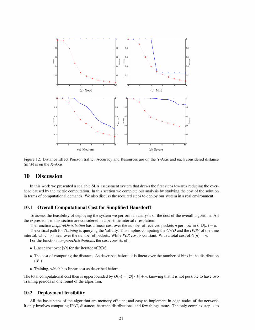
As we already discussed, querying the other end-point to acquire the network status is one of the bottlenecks ofthe system. The querying is triggered when D(D,Q) ≥ δ (Step 6 of Algorithm 2). Hence δ and the traffic itselfdetermine the amount of queries of the system. Figure 12 details the effects of changing δ between 0 and 10% forcontrolled traffic generation with Poissonian Traffic using our algorithm Simplified Hausdorff Distance (the studywould be analogous in the case of Kullback-Leibler and Hausdorff ).

All the subfigures contain the Accuracy in the left Y-Axis with solid line, and the Resources needed on the rightY-Axis with dotted line. The X-Axis contains the different values for δ. As it can be observed, in the case of Goodand Severe traffic conditions, the effects of increasing the distance permits to reduce the required resources given thepredictability of the outcome, specially in the Good case where the estimation is always correct. Again the importanttrade-off is on the fuzzy situation where not much SLA violations occur on the network, in that case, increasing thedistance has a very noticeable effect on the final accuracy of the system, due to the statistical error incurred whenhaving a small number of samples, being more noticeable when there are fewer disruptions (Mild case in the figure).

20

0 2 4 6 8 100

0.2

0.4

0.6

0.8

1

Acc

urac

y

0 2 4 6 8 100

0.2

0.4

0.6

0.8

1

Res

ourc

es

(a) Good

0 2 4 6 8 100

0.2

0.4

0.6

0.8

1

Acc

urac

y

0 2 4 6 8 100

0.2

0.4

0.6

0.8

1

Res

ourc

es

(b) Mild

0 2 4 6 8 100

0.2

0.4

0.6

0.8

1

Acc

urac

y

0 2 4 6 8 100

0.2

0.4

0.6

0.8

1

Res

ourc

es

(c) Medium

0 2 4 6 8 100

0.2

0.4

0.6

0.8

1

Acc

urac

y

0 2 4 6 8 100

0.2

0.4

0.6

0.8

1

Res

ourc

es

(d) Severe

Figure 12: Distance Effect Poisson traffic. Accuracy and Resources are on the Y-Axis and each considered distance(in %) is on the X-Axis

10 DiscussionIn this work we presented a scalable SLA assessment system that draws the first steps towards reducing the over-

head caused by the metric computation. In this section we complete our analysis by studying the cost of the solutionin terms of computational demands. We also discuss the required steps to deploy our system in a real environment.

10.1 Overall Computational Cost for Simplified HausdorffTo assess the feasibility of deploying the system we perform an analysis of the cost of the overall algorithm. All

the expressions in this section are considered in a per-time interval t resolution.The function acquireDistribution has a linear cost over the number of received packets n per flow in t: O(n) = n.The critical path for Training is querying the Validity. This implies computing the OWD and the IPDV of the time

interval, which is linear over the number of packets. While PLR cost is constant. With a total cost of O(n) = n.For the function compareDistributions, the cost consists of:

• Linear cost over |D| for the iterator of RDS.

• The cost of computing the distance. As described before, it is linear over the number of bins in the distribution(|P|).

• Training, which has linear cost as described before.

The total computational cost then is upperbounded by O(n) = |D| · |P|+n, knowing that it is not possible to have twoTraining periods in one round of the algorithm.

10.2 Deployment feasibilityAll the basic steps of the algorithm are memory efficient and easy to implement in edge nodes of the network.

It only involves computing IPAT, distances between distributions, and few things more. The only complex step is to

21

give feedback to the system about the real metrics of the network, because it requires to match packets of the flowsunder analysis on the different edge nodes. This can be performed by using different techniques as described in ourprevious work [1,2] with dedicated boxes forming an overlay network within the network under analysis. Therefore itis removing complexity from the edges.

11 ConclusionsWe have presented a novel approach to on-line SLA Assessment, where differently of previous research, our

work separates and reduces the performance metric computation and the interaction between the edge nodes of thenetwork. This is accomplished by: i) a smart algorithm for gathering the distribution of Inter-Packet Arrival Time(IPAT); ii) distance algorithms to compare the distributions; and iii) a robust Training methodology that delivers a verycompetitive solution regarding SLA violation detection.

As an additional contribution, we improved Hausdorff Distance, by using the knowledge about the data we aredealing with. With this improved version we can efficiently infer the network quality with very good accuracy and avery low amount of resources.

We validated our methodology with a set of different tests, which involved a controlled and European-widetestbeds, using synthetic and real traffic. The experimental results show that we can reduce the required resourcesconsiderably, with a low effect on the final accuracy of the system.

As lines left for further research, an interesting upgrade of the system would be to infer the real metrics of thenetwork by comparing ingress and egress packet arrival times (Inter Packet Generation Time with Inter Packet ArrivalTime).

AcknowledgementsWe would like to thank Marcelo Yannuzzi for all the effort and good advise during this work. We also are in debt

with the EuQoS testbed owners who helped us during the project to perform the tests presented here.

References[1] Rene Serral-Gracia, Pere Barlet-Ros, and Jordi Domingo-Pascual. Coping with Distributed Monitoring of QoS-

enabled Heterogeneous Networks. In 4th International Telecommunication Networking Workshop on QoS inMultiservice IP Networks, pages 142–147, 2008.

[2] Rene Serral-Gracia, Albert Cabellos-Aparicio, and Jordi Domingo-Pascual. Network performance assessmentusing adaptive traffic sampling. IFIP Networking, LNCS 4982:252–263, May 2008.

[3] T. Zseby. Deployment of Sampling Methods for SLA Validation with Non-Intrusive Measurements. Proceedingsof Passive and Active Measurement Workshop (PAM), pages 25–26, 2002.

[4] Joel Sommers, Paul Barford, Nick Duffeld, and Amos Ron. Accurate and Efficient SLA Compliance Monitoring.In Proceedings of ACM SIGCOMM, pages 109–120, 2007.

[5] Y. Labit, P. Owezarski, and N. Larrieu. Evaluation of active measurement tools for bandwidth estimation inreal environment. 3rd IEEE/IFIP Workshop on End-to-End Monitoring Techniques and Services (E2EMON’05),pages 71–85, 2005.

[6] D.A. Vivanco and A.P. Jayasumana. A Measurement-Based Modeling Approach for Network-Induced PacketDelay. Local Computer Networks (LCN). 32nd IEEE Conference on, pages 175–182, 2007.

[7] NM Piratla, AP Jayasumana, and H. Smith. Overcoming the effects of correlation in packet delay measurementsusing inter-packet gaps. Networks (ICON). Proceedings. 12th IEEE International Conference on, 1, 2004.

[8] Paul Barford and Joel Sommers. Comparing probe -and router- based methods for measuring packet loss. IEEEInternet Computing, Special Issue on Measuring the Internet, 2004.

22

[9] Joel Sommers, Paul Barford, Nick Duffeld, and Amos Ron. Improving Accuracy in End-to-end Packet LossMeasurement. In Proceedings of ACM SIGCOMM, 2005.

[10] Andrew McCallum, Don Towsley, and Yu Gu. Detecting Anomalies in Network Traffic Using Maximum EntropyEstimation. In Internet Measurement Conference (IMC), pages 345–350, 2005.

[11] Yann Labit and J. Mazel. HIDDeN: Hausdorff distance based Intrusion Detection approach DEdicated to Net-works. In The Third International Conference on Internet Monitoring and Protection (ICIMP 2008), Bucharest(Romania), pages 11–16, 29 June - 5 July 2008.

[12] S. Kullback and R.A. Leibler. On information and sufficiency. Annals of Mathematical Statistics, 22(1):79–86,1951.

[13] E. Baudrier, N. Girard, and J.M. Ogier. A non-symmetrical method of image local-difference comparison forancient impressions dating. Workshop on Graphics Recognition (GREC), 2007.

[14] MJ Atallah. Linear time algorithm for the Hausdorff distance between convex polygons. INFO. PROC. LETT.,17(4):207–209, 1983.

[15] O. Jesorsky, K.J. Kirchberg, R. Frischholz, et al. Robust face detection using the hausdorff distance. Proceedingsof Audio and Video based Person Authentication, pages 90–95, 2001.

[16] P. Owezarski, P. Berthou, Y. Labit, and D. Gauchard. LaasNetExp: a generic polymorphic platform for net-work emulation and experiments. Proceedings of the 4th International Conference on Testbeds and researchinfrastructures for the development of networks & communities, 2008.

[17] IST-EuQoS – End-to-end Quality of Service support over heterogeneous networks - http://www.euqos.eu/,September 2004.

23

Documents

Distance based Service Level Agreement assessment