Turk J Math

(2017) 41: 1404 – 1432

c⃝ TUBITAK

doi:10.3906/mat-1610-83

Turkish Journal of Mathematics

http :// journa l s . tub i tak .gov . t r/math/

Research Article

Dissipative operator and its Cayley transform

Ekin UGURLU∗, Kenan TASDepartment of Mathematics, Faculty of Arts and Sciences, Cankaya University, Ankara, Turkey

Received: 21.10.2016 • Accepted/Published Online: 10.01.2017 • Final Version: 23.11.2017

Abstract: In this paper, we investigate the spectral properties of the maximal dissipative extension of the minimal

symmetric differential operator generated by a second order differential expression and dissipative and eigenparameter

dependent boundary conditions. For this purpose we use the characteristic function of the maximal dissipative operator

and inverse operator. This investigation is done by the characteristic function of the Cayley transform of the maximal

dissipative operator, which is a completely nonunitary contraction belonging to the class C0. Using Solomyak’s method

we also introduce the self-adjoint dilation of the maximal dissipative operator and incoming/outgoing eigenfunctions of

the dilation. Moreover, we investigate other properties of the Cayley transform of the maximal dissipative operator.

Key words: Cayley transform, completely nonunitary contraction, unitary colligation, characteristic function, CMV

matrix

1. Introduction

If an operator T1 acting on a Hilbert space H1 is equivalent to another operator T2 acting on another Hilbert

space H2 in a certain sense, then one can say that T2 is a model of T1. There exist models up to unitary

equivalence, similarity equivalence, quasi-similarity, pseudo-similarity, and other equivalences [27]. A useful

model was given by Sz.-Nagy and Foias [24, 25]. Sz.-Nagy and Foias constructed the model operator for the

contractive operators acting on Hilbert spaces. This construction is based on the dilation. An operator U acting

on a Hilbert space H is called a dilation of an operator T acting on a Hilbert space H such that H ⊂ H if

Tnf = PHUnf, f ∈ H, n ≥ 0,

where PH is the orthogonal projection of H onto H, and H is called the dilation space. If U is unitary on

H , then U is called unitary dilation of T. Moreover, if the minimal subspace of H containing H and being

invariant with respect to U and U∗ coincides with H , then U is called minimal. In 1965, Sarason gives the

geometric structure of the dilation space [32]. In fact, Sarason showed that an operator U acting on H is a

dilation of its compression PHU | H if and only if H decomposes in the following way

H = G∗ ⊕H ⊕G,

where UG ⊂ G and U∗G∗ ⊂ G∗. Moreover, if an operator T has a unitary dilation then T is a contraction,

i.e. ∥T∥ ≤ 1. The geometric structure of the dilation space allows one to give a more useful description of the

∗Correspondence: ekinugurlu@cankaya.edu.tr

2010 AMS Mathematics Subject Classification: Primary 47B36; Secondary 47B44, 47A48, 34B20, 62M15

1404

UGURLU and TAS/Turk J Math

minimal unitary dilation of a contraction. Namely, if U is a minimal unitary dilation on H = G∗ ⊕H ⊕G of

contraction T acting on H, then

U =

PG∗U | G∗ 0 0DT∗V ∗

∗ T 0−V T ∗V ∗

∗ V DT U | G

,

where DT∗ = (I − TT ∗)1/2, DT = (I − T ∗T )1/2, V is a partial isometry with initial space DT = DTH

and final space E = G ⊖ UG and V∗ is a partial isometry with initial space DT∗ = DT∗H and final space

E∗ = G∗ ⊖ U∗G∗. Note that an operator V : H → K is called partial isometry if H = Hi ⊕ H0 , where

V : Hi → H is an isometry and V | H0 = 0. Hi is called the initial space of V and its range V Hi = V H the

final space of V.

Another description of the dilation U of contraction T can be given with the following unitary mappings

U | span (Un (G⊖ UG) : n ∈ Z) = U |⊕n∈Z

Un (G⊖ UG) ,

U | span (Un (G∗ ⊖ U∗G∗) : n ∈ Z) = U |⊕n∈Z

Un (G∗ ⊖ U∗G∗) .

Let us consider the spaces E and E∗ such that

dimE = dim (G⊖ UG) , dimE∗ = dim (G∗ ⊖ U∗G∗) .

Then the unitary mappings given above are the multiplication operators g(z) → zg(z) on L2(E) and L2(E∗),

respectively. Let

υ : E → G⊖ UG, υ∗ : E∗ → G∗ ⊖ U∗G

be the unitary mappings and

∏: L2(E)⊕ L2(E∗) → H,

(f, g) → πf + π∗g,

where

π : L2(E) →⊕n∈Z

Un(G⊖ UG),∑nznen →

∑nUnυen,

and

π∗ : L2(E∗) →⊕n∈Z

Un(G∗ ⊖ U∗G∗),∑nzne∗n →

∑nUn+1υ∗e

∗n.

The operators π and π∗ are called functional embeddings. The function

π∗∗π = Θ : E → E∗

is called the characteristic function of the contraction T. An explicit formula for the characteristic function is

given as

1405

UGURLU and TAS/Turk J Math

ΘT (z)h = V∗(−T + zDT∗(I − zT ∗)−1DT )V∗h, h ∈ E,

where V and V∗ are the unitary identifications such as

V : DT ↔ E, V∗ : DT∗ ↔ E∗.

If one chooses E = DT and E∗ = DT∗ , then ΘT is reduced to

ΘT = −T + zDT∗(I − zT ∗)−1DT ,

which is the well-known characteristic function given by Sz.-Nagy and Foias.

An operator B with domain D(B) acting on a Hilbert space H is called dissipative if

Im(By, y) ≥ 0, y ∈ D(B)

and accumulative if

Im(By, y) ≤ 0, y ∈ D(B).

There is a connection between dissipative operators and contractions. Indeed, the Cayley transform of a

dissipative operator defines a contraction. Solomyak used this connection and free parameters to obtain the

characteristic function of the maximal dissipative operator [35]. For this purpose, Solomyak used the boundary

spaces of the maximal dissipative operator. Indeed, let B be a maximal dissipative operator, GB be its

Hermitian part, and P be the natural projection defined on the quotient space such as P : D(B) → D(B)/GB .

The completion F (B) of the quotient space D(B)/GB is called the boundary space. Similarly, F∗(B) is defined

as F∗(B) = F (−B∗). Moreover, P∗ is defined from D(B∗) onto D(B∗)/GB . Then Solomyak introduced the

connection of the characteristic functions between the maximal dissipative operator B and its Cayley transform

T as

SB(λ) = ΘT

(λ− i

λ+ i

), Imλ > 0

with the rule

SB(λ) = P∗(B∗ − λI)−1(B − λI)P−1.

Moreover, with the help of free parameters Solomyak constructed a self-adjoint dilation of the maximal dissi-

pative operator. Using the characteristic function he described directly the generalized eigenfunctions of the

self-adjoint dilation.

In this paper, we investigate the spectral properties of the maximal dissipative extension generated by a

second order differential expression in the limit-circle case and two boundary conditions in which the domain of

the minimal symmetric operator contains a spectral parameter in the boundary conditions. To indicate that the

extension is maximal dissipative we use Gorbachuks’ theorem on extension, which requires the equal deficiency

indices [19]. Although the second order differential expression is in the limit-circle case, the minimal symmetric

operator has the deficiency indices (1, 1). This connection has been studied by Maozhu et al. in [22]. On the

other hand, it is known that any symmetric operator with deficiency indices (n, n) has a boundary value space

1406

UGURLU and TAS/Turk J Math

with dimension n. Therefore, this relation allows us to construct a maximal dissipative extension of the minimal

symmetric operator.

The investigation of the spectral properties of the maximal dissipative operator is based on the charac-

teristic function and the inverse operator of the maximal dissipative operator. Using the connection between

the characteristic functions of the maximal dissipative operator and its Cayley transform we obtain the charac-

teristic function of the Cayley transform. We also prove that the Cayley transform is a completely nonunitary

(c.n.u.) contraction belonging to the class C0 , which consists of those c.n.u. contractions T for which there

exists a nonzero function u ∈ H∞ (Hp denotes the Hardy class) such that u(T ) = 0. It is well known that

u has a canonical factorization into the product of an inner function ui and outer function ue. The equation

u(T ) = 0 implies that ui(T ) = 0 and therefore one may ask whether for a c.n.u. contraction T belonging to the

class C0 there exists an inner function u with u(T ) = 0 such that every other function v ∈ H∞ with v(T ) = 0

is a multiple of u. Such a function mT is called a minimal function of T and this function is determined up to

a constant factor of modulus one. Sz.-Nagy and Foias proved that for every contraction T ∈ C0 there exists a

minimal function mT . With the help of mT , some spectral properties of T ∈ C0 can be obtained. For example,

the spectrum of the contraction T ∈ C0 and the zeros of the minimal function mT in the open disc D and

of the complement, in the unit circle C, of the union of the arcs of C on which mT is analytic, coincide with

each other. Moreover, the points of the spectrum in the interior of the unit circle C are eigenvalues of T. As a

characteristic value of T , λ has finite index, equal to its multiplicity as a zero of mT . Completeness of the root

vectors of T associated with the points of the spectrum of T in D can be proved as showing that the minimal

function mT is a Blaschke product.

We should note that this method is new and differs from Pavlov’s method [1–6, 30, 31, 36]. In fact,

Pavlov’s method is based on the fact that there is a connection between a continuous semigroup of contractions

Z(t)t≥0 and its cogenerator Z. Therefore every model of Z generates a model of Z(t)t≥0 . In this paper,

we only use the Cayley transform of the maximal dissipative operator.

For an arbitrary bounded operator it is important to find the least subspace that is a generating subspace

for the bounded operator. The dimension of such a subspace is called the spectral multiplicity or multiplicity

of the bounded operator. The characteristic function may help one to find the multiplicity of the contraction.

Therefore we find the multiplicity of the contraction of the maximal dissipative operator.

It is known that unitary colligation theory is more general than the characteristic function theory of

contractions given by Sz.-Nagy and Foias. Since the Cayley transform of our maximal dissipative operator has

finite defect indices, embedding the contraction to its unitary colligation we introduce some results with the

help of the results reported by Arlinskiı et al. [10].

Jacobi matrices are useful to understand the characterization of self-adjoint, nonself-adjoint, and unitary

operators acting on separable Hilbert spaces. Indeed, multiplication operators on the Hilbert spaces L2(R) or

L2(C) associated with the probability measure m on the real line R or on the unit circle C , respectively, are

unitary equivalent to the self-adjoint or unitary operators with a simple spectrum acting on some Hilbert spaces

[8]. Tri-diagonal Jacobi matrix representation of self-adjoint operators with simple spectrum was introduced by

Stone [9]. The nonself-adjoint version of Stone’s theorem has been introduced by Arlinskiı and Tsekanovskiı [11].

Moreover, the canonical matrix representation of unitary operators with simple spectrum has been introduced

by Cantero et al. [15] with the help of five-diagonal unitary matrices called CMV matrices. Arlinskiı et al. [10]

obtained a connection between truncated CMV matrix and Sz.-Nagy-Foias characteristic function. Therefore,

we introduce a truncated CMV matrix associated with the Cayley transform.

1407

UGURLU and TAS/Turk J Math

This paper is organized as follows. In section 2, we construct the maximal dissipative extension of the

minimal symmetric differential operator. In section 3, passing to the Cayley transform of the dissipative operator

we obtain a contraction. Moreover, we find the characteristic functions of the maximal dissipative operator and

its Cayley transform and using the properties of the Cayley transform and its characteristic function we introduce

some results about the spectral analysis of both the maximal dissipative operator and its Cayley transform.

In section 4, we obtain the inverse operator of the dissipative operator, which is an integral operator with

finite-rank imaginary component. Then we introduce the complete spectral analysis of the dissipative operator.

In section 5, we construct the self-adjoint dilation and its incoming/outgoing eigenfunctions directly. In section

6, we introduce some results on the Cayley transform of the dissipative operator.

Finally we should note that the notations C and D will be used to describe the unit circle C = µ :

|µ| = 1 and unit disc D = µ : |µ| < 1 .

2. Maximal dissipative extension of the minimal symmetric operator

In this paper we consider the following second order differential equation:

ℓ(y) = λy, x ∈ I, (2.1)

where

ℓ(y) =1

w(x)[−(p(x)y′)′ + q(x)y] ,

I = [a, b), −∞ < a < b ≤ ∞ , and λ is a complex parameter. We assume that a is the regular point and b

is the singular point for the equation (2.1), p, q, w are real-valued Lebesgue measurable functions on I, p−1, q

and w are locally integrable functions on I and w > 0 for almost all x ∈ I.Let L2

w(I) denote the Hilbert space consisting of all functions y satisfying∫I

|y|2 wdx < ∞

with the inner product

(y, χ) =

∫I

yχwdx.

We denote by M a subset of L2w(I) that consists of those functions y ∈ L2

w(I) such that y and py′ are

locally absolutely continuous functions on I and ℓ(y) ∈ L2w(I). The operator L , defined by Ly = ℓ(y), y ∈ M,

is called the maximal operator with domain M. Let L∗ = L0 with domain M0 . The set M0 consists of those

functions y ∈ M satisfying y(a) = (py′)(a) = 0 and [y, χ](b) = 0 for all χ ∈ M.

The deficiency indices of the minimal operator L0 are defined as the numbers (m,n) such that

m = dim((L0 − λI

)D(L0)

)⊥, n = dim ((L0 − λI)D(L0))

⊥,

where D(L0) is the domain of L0 and λ is the complex number . It is well known that L0 is self-adjoint if

and only if m = n = 0 and L0 has self-adjoint extensions if and only if m = n . (1, 1) is known as Weyl’s

limit-point case and (2, 2) is known as Weyl’s limit-circle case for a second order operator.

1408

UGURLU and TAS/Turk J Math

In this paper, we assume that w, p and q satisfy Weyl’s limit-circle case conditions at singular point b.

In other words, we assume that the deficiency indices of L0 are (2, 2) [12, 17, 20, 26, 38].

For two arbitrary functions y, χ ∈ M the following Green’s formula holds∫I

ℓ(y)χ− yℓ(χ)wdx = [y, χ](b)− [y, χ](a),

where [y, χ](x) := y(x)χ[1](x) − y[1](x)χ(x) and y[1] = py′. Green’s formula implies that for arbitrary two

functions y, χ ∈ M, the values [y, χ](b) and [y, χ](b) exist and are finite. The secondary one follows from the

fact that p, q and w are real valued functions on I.Let u and v be the real solutions of the equation ℓ(y) = 0, x ∈ I, satisfying the conditions

u(a) = α2, u[1](a) = α1, v(a) = γ2, v[1](a) = γ1, (2.2)

such that [u, v](a) = 1. Moreover, Green’s formula and (2.2) imply that [u, v] = 1 for all x ∈ I. Therefore for

two arbitrary functions y, χ ∈ M one has

[y, χ] = [y, u][χ, v]− [y, v][χ, u], x ∈ I. (2.3)

Since the limit-circle case holds for ℓ, u and v belong to L2w(I) and M. Therefore for arbitrary y ∈ M ,

the values [y, u](b) and [y, v](b) exist and are finite.

For y ∈ M, we consider the following boundary conditions:

α1y(a)− α2y[1](a) = λ

(β1y(a)− β2y

[1](a)),

[y, v](b) + h[y, u](b) = 0,(2.4)

where α1, α2, β1, β2 are real numbers such that δ := β1α2 − β2α1 > 0 and h is a complex number such that

h = h1 + ih2 with h2 > 0.

Let H = L2w(I)⊕ C be the Hilbert space with the inner product

⟨Y,Z⟩H = (y, z) +1

δy1z1,

where

Y =

(y(x)y1

),Z =

(z(x)z1

)∈ H.

We consider the set D(L) consisting of all functions Y =(yy1

)such that y ∈ M satisfying y1 =

β1y(a)− β2y[1](a). Let L be the operator defined on D(L) with the rule

LY =

(ℓ(y)

α1y(a)− α2y[1](a)

).

Let D(L0) be the set consisting of all functions Y ∈ D(L) such that [y, z](b) = 0 for all

Z =

(z(x)z1

)∈ H.

1409

UGURLU and TAS/Turk J Math

The operator L0 is defined as the restriction of the operator L to the set D(L0). It is known that L0 is closed,

densely defined, symmetric, and L∗0 = L in H [22] . Moreover, since L0 has the deficiency indices (2, 2), the

deficiency indices of L0 are (1, 1) [22].

Recall that [19] a triple (H,Γ1,Γ2), where H is a Hilbert space and Γ1,Γ2 are linear mappings of D(A∗)

into H, is called a boundary value space of the operator A if,

(i) for any f, g ∈ D(A∗),

(A∗f, g)− (f,A∗g) = (Γ1f,Γ2g)H − (Γ2f,Γ1g)H,

(ii) for any F1, F2 ∈ H there exists a vector f ∈ D(A∗) such that Γ1f = F1,Γ2f = F2.

Theorem 2.1. [19] For any symmetric operator with deficiency indices (n, n) (n ≤ ∞) there exists a boundary

value space (H,Γ1,Γ2) with dimH = n.

Now consider the following linear mappings:

Γ1Y = [y, u](b), Γ2Y = [y, v](b).

Then we have the following theorem.

Theorem 2.2. (C,Γ1,Γ2) is a space of boundary values of L0.

Proof Let Y ∈ D(L). Then y ∈ M and for any complex numbers c1 and c2 , the values [y, u](b) = c1 and

[y, v](b) = c2 exist [1, 2, 26]. Moreover, for Y,Z ∈ D(L) one gets

⟨L∗0Y,Z⟩H − ⟨Y,L∗

0Z⟩H = [y, z](b). (2.5)

On the other hand, we have

(Γ1Y,Γ2Z)C − (Γ2Y,Γ1Z)C = [y, z](b). (2.6)

Therefore (2.5) and (2.6) complete the proof. 2

The following theorem, given by Gorbachuks, describes all maximal dissipative maximal accumulative

and maximal self-adjoint extension of a given minimal symmetric operator.

Theorem 2.3. [19] If K is a contraction on H, then the restriction of the operator A∗ to the set of vectors

f ∈ D(A∗) satisfying the condition

(K − I) Γ1f + i (K + I) Γ2f = 0, (2.7)

or(K − I) Γ1f − i (K + I) Γ2f = 0, (2.8)

is a maximal dissipative, respectively, a maximal accumulative extension of A. Conversely, any maximal

dissipative (maximal accumulative) extension of A is the restriction of A∗ to the set of vectors f ∈ D(A∗)

satisfying (2.7) ((2.8)), where a contraction K is uniquely determined by an extension. The maximal symmetric

extensions of an operator A on H are described by the conditions (2.7) ((2.8)), where K is a isometric operator.

These conditions define a self-adjoint extension if K is unitary. In the last case (2.7), (2.8) are equivalent to

(cosC)Γ2f − (sinC)Γ1f = 0,

1410

UGURLU and TAS/Turk J Math

where C is a self-adjoint operator on H. The general form of dissipative (accumulative) extension of A is given

by the condition

K(Γ1f + iΓ2f) = Γ1f − iΓ2f, Γ1f + iΓ2f ∈ D(K), (2.9)

respectively,

K(Γ1f − iΓ2f) = Γ1f + iΓ2f, Γ1f − iΓ2f ∈ D(K), (2.10)

where K is a linear operator satisfying ∥Kf∥ ≤ ∥f∥ (f ∈ D(K)), while symmetric extensions are described by

the formulas (2.9) and (2.10), where K is an isometric operator.

Therefore Theorems 2.2 and 2.3 give the following.

Theorem 2.4. All maximal dissipative extensions of the operator L0 are given by the boundary condition

[y, v](b) + h[y, u](b) = 0, y ∈ M, (2.11)

where h is a complex number as h = h1 + ih2 with h2 > 0.

Let D(Lh) be the set consisting of all functions Y ∈ D(Lh) satisfying (2.11). We define the operator Lh

on D(Lh) with the rule

LhY = LY, Y ∈ D(Lh).

Therefore Lh is the maximal dissipative extension of L0 and the equation

LhY = λY

coincides with the problem (2.1), (2.4).

Definition 2.5. A nonself-adjoint operator L acting on a Hilbert space H is called simple if there is no

invariant subspace of H on which L has a self-adjoint part there.

Theorem 2.6. Lh is simple on H.

Proof Let Hs be a subspace of H on which Lh has a selfadjoint part there. For Y ∈ D(Lh) ∩Hs one gets

0 = ⟨LhY,Y⟩Hs− ⟨Y,LhY⟩Hs

= 2ih2 |[y, u](b)|2 .

Therefore [y, u](b) = 0 and hence [y, v](b) = 0. This implies that y ≡ 0 on [a, b) and y1 = 0. Consequently

Y ≡ 0. This completes the proof. 2

Let us consider the solution φ(x, λ) of the equation (2.1) satisfying the conditions

φ(a, λ) = α2 − λβ2, φ[1](a, λ) = α1 − λβ1.

Then the zeros of the function

∆h(λ) = [φ(x, λ), v(x)](b) + h[φ(x, λ), u(x)](b)

coincide with the eigenvalues of Lh. It can be obtained that ∆h is an entire function of λ of order ≤ 1 of

growth and of minimal type. Therefore the eigenvalues of Lh are purely discrete and possible limit points of

these eigenvalues can only occur at infinity. However, more detailed analysis will be obtained with the help of

the characteristic function and inverse operator Lh.

1411

UGURLU and TAS/Turk J Math

3. Characteristic function

The following lemma gives a nice connection between maximal dissipative operators and related contractions

[24, 25, 35].

Lemma 3.1. (i) Assume the operator L0 is dissipative. Then the operator T0 = K(L0) = (L0 −iI)(L0 + iI)−1 is a contraction from (L0 + iI)D(L0) onto (L0 − iI)D(L0) and L0 = i(I + T0)(I − T0)

−1.

For each contraction T0 such that 1 /∈ σp(T0) (the point spectrum of the operator), operator L0 = K−1(T0),

D(L0) = (I − T0)D(T0), is dissipative.

(ii) Each dissipative operator L0 has a maximal dissipative extension L. A maximal dissipative operator

is closed.

(iii) A maximal dissipative operator is maximal dissipative if and only if T = K(L) is a contraction such

that D(T ) = H and 1 /∈ σp(T ).

(iv) If L is a maximal dissipative operator, L = K−1(T ), then −L∗ is also maximal dissipative,

L∗ = −K−1(T ∗).

(v) If L is a maximal dissipative operator, then σ(T ) ⊂ C+,∥∥(L− λI)−1

∥∥ ≤ |Imλ|−1, λ ∈ C−.

For a maximal dissipative operator B with domain D(B), the subspace

GB = y ∈ D(B) ∩D(B∗) : By = B∗y

is called the Hermitian part of the domain of B.

Let P be the natural projection defined as

P : D(B) → D(B)/GB,

where D(B)/GB is the quotient space. On the quotient space the following inner product is defined

⟨Py,Pχ⟩ = i

2((y,Bχ)− (By, χ)) , y, χ ∈ D(B).

We denote by F (B) the completion of the quotient space D(B)/GB with respect to the corresponding

norm. Similarly, we define F∗(B) as F∗(B) = F (−B∗). Here the projection P∗ is defined as

P∗ : D(B∗) → D(B∗)/GB .

Therefore we have

∥Py∥2F = Im(By, y), ∥P∗z∥2F∗= −Im(B∗z, z). (3.1)

F (B) and F∗(B) are Hilbert spaces and are called boundary spaces of the operator B.

We have from (3.1) that

∥PY∥2F = h2 |[y, u](b)|2 , ∥P∗Z∥2F = h2 |[z, u](b)|2 .

Note that if one has all dissipative extensions of a symmetric operator B, then GB is dense in the Hilbert

space. If y ∈ D(B) ∩D(B∗), then By = B∗y, i.e. D(B) ∩D(B∗) = GB.

Let Ch be the Cayley transform of the dissipative operator Lh as Ch = (Lh − i1)(Lh + i1)−1 from

(Lh + i1)D(Lh) onto (Lh − i1)D(Lh), where 1 is the identity operator in the direct sum Hilbert space H.

1412

UGURLU and TAS/Turk J Math

Since Lh is maximal dissipative, the domain of Ch is the Hilbert space H. Let DCh= (1− C∗

hCh)1/2

and

DC∗h= (1− ChC∗

h)1/2

be the defect operators of Ch acting on H, DCh= DCh

H and DC∗h= DC∗

hH be the defect

spaces, and dCh= dimDCh

and dC∗h= dimDC∗

hbe the defect indices of Ch.

Definition 3.2. A contraction C on a Hilbert space H is called c.n.u. if for no nonzero reducing subspace Cfor C is C | C is a unitary operator.

For (Lh + i1)F = Y, the inequality

∥(Lh − i1)Y∥2H < ∥(Lh + i1)Y∥2H (3.2)

holds if and only if

2Im ⟨LhY,Y⟩H > 0.

Particularly, (3.2) shows

∥Ch∥H < 1. (3.3)

Note that 1 cannot belong to the point spectrum of Ch [24, 25, 35]. On the other hand,

Lh = i(1+ Ch)(1− Ch)−1.

However, this does not imply that Lh is a bounded operator (see [25], p. 171).

From (3.3) one gets the following.

Theorem 3.3. Ch is a c.n.u. contraction in H.

It is known that there exist isometric isomorphisms between F (Lh) (F∗(Lh)) and DCh(DC∗

h). Indeed,

the mappings ρ : F (Lh) → DChand ρ∗ : F∗(Lh) → DC∗

h[35] such that

ρP(1− Ch) = DCh, ρ∗P∗(1− C∗

h) = DC∗h

define isometric isomorphism.

A c.n.u. contraction T is defined to within a unitary equivalence of the characteristic function

ΘT : E → E∗,

where E and E∗ are auxiliary Hilbert spaces, isomorphic to DChand DC∗

h, respectively. Fixing isometric

isomorphisms Ω : E → DCh, Ω∗ : E∗ → DC∗

h, one has

ΘCh(µ) = Ω∗

∗(−Ch + µDC∗

h(1− µC∗

h)DCh

)Ω

and

ΘCh(µ)Ω∗DCh

= Ω∗∗DC∗

h(1− µC∗

h)−1(µ1− Ch),

where µ ∈ D.

1413

UGURLU and TAS/Turk J Math

For a simple maximal dissipative operator B and its Cayley transform T , the characteristic function of

B is defined as

SB(λ) = ΘT

(λ− i

λ+ i

), Imλ > 0. (3.4)

The characteristic function SB : F (B) → F∗(B) on the sense set D(B)/GB is defined by

SB(λ) = P∗(B∗ − λI)−1(B − λI)P−1. (3.5)

Therefore we have the following theorem.

Theorem 3.4. The characteristic function of Lh is as follows

SLh(λ) =

∆h(λ)

∆h(λ).

Proof Since Lh is a dissipative extension of the symmetric operator L0 , we have GLh= D(Lh) ∩ D(L∗

h).

Moreover, F (Lh) = D(Lh)/GLhand F∗(Lh) = D(L∗

h)/GLh.

Let P and P∗ be the natural projections such that P : D(Lh) → F (Lh) and P∗ : D(L∗h) → F∗(Lh).

We set E = E∗ = C and we define the isometric isomorphisms Ψ and Ψ∗ such as

Ψ : E → F (Lh),a → Ψ(a) = PY,

(3.6)

where Y ∈ D(Lh) with

[y, u](b) =a√h2

and

Ψ∗ : E∗ → F∗(Lh),a → Ψ∗(a) = P∗Z,

(3.7)

where Z ∈ D(L∗h) with

[z, u](b) =a√h2

.

Using (3.5) we obtain the characteristic function SLhas

SLh(λ) = Ψ∗

∗P∗(L∗h − λ1)−1(Lh − λ1)P−1Ψ. (3.8)

Therefore (3.6) and (3.8) give

SLh(λ)a = Ψ∗

∗P∗Z,

where

Z = (L∗h − λ1)−1(Lh − λ1)Y, Y ∈ D(Lh) (3.9)

with [y, u](b) = a/√h2. Moreover, (3.7) implies that

Ψ∗∗P∗Z = [z, u](b)

√h2.

1414

UGURLU and TAS/Turk J Math

Therefore using (3.8) one can write

SLh(λ)a =

[z, u](b)

[y, u](b)a. (3.10)

(3.9) implies that

(L∗h − λ1)Z = (Lh − λ1)Y,

where Z ∈ D(L∗h) and Y ∈ D(Lh). Consequently, one should find a solution of the equation

−(pκ′)′ + qκ = λκ,

from the space L2w(I) subject to the condition

α1κ(a)− α2κ[1](a) = λ(β1κ(a)− β2κ[1](a)

),

where κ = z − y such that κ =(κ(x,λ)

κ1

)and κ1 = β1κ(a, λ)− β2κ[1](a, λ).

Let

φ =

(φ(x, λ)φ1

),

where φ1 = β1φ(a, λ)− β2φ[1](a, λ). Then one can infer that κ = cφ, where c is a constant.

From the equation

[φ, v](b) =[φ, v](b)

[φ, u](b)[φ, u](b)

we obtain

[z, u](b)([φ, v](b) + h[φ, u](b)

)= [y, u](b) ([φ, v](b) + h[φ, u](b)) . (3.11)

Substituting (3.11) into (3.10) we complete the proof. 2

Now using (3.4) we obtain the following theorem.

Theorem 3.5. The characteristic function of Ch is as follows:

ΘCh(µ) =

∆h(λ)

∆h(λ), µ =

λ− i

λ+ i, Imλ > 0.

Since there is a connection between the characteristic functions of Ch and C∗h with the rule

ΘC∗h(µ) = Θ∗

Ch(µ) , µ ∈ D,

we obtain the following corollary.

Corollary 3.6. The characteristic function of C∗h is

ΘC∗h(µ) =

∆h

(−i 1+µ

1−µ

)∆h

(−i 1+µ

1−µ

) , µ =λ− i

λ+ i, Imλ > 0.

1415

UGURLU and TAS/Turk J Math

Remark 3.7. Since Ch is a c.n.u. contraction, 1 cannot belong to the point spectrum of Ch. On the other

hand, the spectrum of Ch coincides with those µ belonging to the disc D for which the operator ΘCh(µ) is not

boundedly invertible, together with those µ ∈ C not lying on any of the open arcs of C on which ΘCh(µ) is a

unitary operator valued analytic function of µ and point spectrum of Ch coincides with those µ ∈ D for which

ΘCh(µ) is not invertible at all. Since the zeros of ∆h(λ), Imλ > 0, are eigenvalues of Lh , λ = i(1+µ)/(1−µ)

for λ = is, lims→∞(is) =: λ∞ cannot be a zero of ∆h(λ) or equivalently an eigenvalue of Lh.

Definition 3.8. [24, 25, 28, 29] The classes C0. and C.0 of contractions are defined as

T ∈ C0. if Tnf → 0 for all f,

T ∈ C.0 if T ∗nf → 0 for all f.

Asymptotic classifications of C0. and C.0 are given as

C0. = T : ∥T∥ ≤ 1, limn ∥Tnf∥ = 0 for every f ,C.0 = T : ∥T∥ ≤ 1, limn ∥T ∗nf∥ = 0 for every f .

C00 is defined as C00 = C0. ∩ C.0.

Theorem 3.9. Ch ∈ C00.

Proof The inequality

∥CnhF∥H ≤ ∥Ch∥nH ∥F∥H

and (3.3) give that Ch ∈ C0.. Since ∥Ch∥H = ∥C∗h∥H one arrives at Ch ∈ C.0. This completes the proof. 2

Remark 3.10. Since Ch ∈ C.0, ΘCh(µ) is an inner function.

Lemma 3.11. dCh= dC∗

h= 1.

Proof Let (Lh + i1)Y = F , where Y ∈ D(Lh), F ∈ H. Then using the idea of [28] we obtain

D2ChF = (Lh + i1)Y − (L∗

h + i1)Z, (3.12)

where Z ∈ D(L∗h) and

Z = (L∗h − i1)

−1(Lh − i1)Y. (3.13)

From (3.13) one infers that

(L∗h − i1)Z = (Lh − i1)Y.

Then we have

D2ChF = (Lh + i1) (Y − Z) = 2icφ(i, λ).

Therefore DChis spanned by φ(i, λ). Namely, the equation

−(pκ′)′ + qκ = 2icκ,

has two linearly independent solutions belonging to L2w(I). However, only one of them satisfies the condition

α1κ(a)− α2κ[1](a) = 2ic(β1κ(a)− β2κ[1](a)

).

1416

UGURLU and TAS/Turk J Math

This solution can be regarded as a multiple of φ(i, λ). Consequently, dCh= 1.

Now let (L∗h − i1)Y = F , where Y ∈ D(L∗

h), F ∈ H. Then

D2C∗hF = (L∗

h − i1)Y − (Lh − i1)Z,

where Z ∈ D(Lh) and

Z = (Lh + i1)−1

(L∗h + i1)Y.

Consequently a similar argument shows that DC∗his spanned by φ(−i, λ), i.e., dC∗

h= 1. Therefore the proof is

completed. 2

Theorems 3.9 and 3.11 give the following theorem.

Theorem 3.12. The c.n.u. contraction Ch belongs to the class C0. Moreover, the characteristic function

ΘCh(µ) of Ch coincides with the minimal function mCh

(µ) of Ch.

Theorem 3.13. ΘChis a Blaschke product in the disc D.

Proof According to Remark 3.10, ΘChcan be represented as

ΘCh(λ) = B(λ) exp(iλb), b > 0, Imλ > 0,

where B(λ) is a Blaschke product in the upper half-plane. Hence we get

|ΘCh(λ)| ≤ exp(−bImλ). (3.14)

For λs = is from (3.14) we get that ∆h(λ) → 0 as s → ∞. Therefore λ∞ = lims→∞ is is a zero of

∆h(λ) or equivalently is an eigenvalue of Lh. However, according to Remark 3.7 this is not possible. Therefore

there cannot be a singular factor in the factorization of ΘCh(λ), Imλ > 0. Letting µ = (λ− i)/(λ+ i) the proof

is completed. 2

According to the well-known theorem given by Sz.-Nagy and Foias we can introduce the following theorem.

Theorem 3.14. Root functions of Ch associated with the points of the spectrum of Ch in D span the Hilbert

space H.

Definition 3.15. Let all root functions of the operator A span the Hilbert space H . Such an operator is called

a complete operator. If every A− invariant subspace is generated by root vectors of A belonging to the subspace

then it is said A admits spectral synthesis.

It is well known that any complete operator belonging to the class C0 admits spectral synthesis [28, 29].

Therefore the following theorem is obtained.

Theorem 3.16. Ch admits spectral synthesis.

There is a connection between the completeness of the root functions of a linear operator and its Cayley

transform [13] (p. 42). Therefore we obtain the following.

Theorem 3.17. Root functions of Lh associated with the point spectrum of Lh in the open upper half-plane

Imλ > 0 span the Hilbert space H.

More detailed analysis of the spectrum of Lh will be obtained with the help of the inverse operator of

Lh in the next section.

1417

UGURLU and TAS/Turk J Math

4. Bounded integral operator with finite-rank imaginary component

In this section we find the inverse operator of Lh. For this purpose let us consider the equality

LhY = F , (4.1)

where

Y =

(yy1

)∈ D(Lh), F =

(ff1

)∈ H.

Equation (4.1) is equivalent to the nonhomogeneous equation

ℓ(y) = f(x), x ∈ I, (4.2)

subject to the conditions

α1y(a)− α2y[1](a) = f1,

[y, v](b) + h[y, u](b) = 0.(4.3)

Let us consider the solutions u and τ = v+ hu. Then the method of variation of parameters gives the solution

y of (4.2), (4.3) as the form

y(x) =

∫I

G(x, t)f(t)w(t)dt− f1τ(x). (4.4)

where

G(x, t) =

−τ(x)u(t), a ≤ t ≤ x−τ(t)u(x), x ≤ t ≤ b

. (4.5)

On the other hand, from (4.5) one obtains

G1(x) = β1G(x, a)− β2G[1](x, a) = −δτ(x). (4.6)

Therefore substituting (4.6) in (4.4) we get that

y(x) =

∫I

G(x, t)f(t)w(t)dt+G1(x)f1

δ

or

y(x) =⟨G(x, t),F(t)

⟩H,

where

G(x, t) =(

G(x, t)G1(x)

).

If we define the operator K as

KF =⟨G(x, t),F(t)

⟩H, (4.7)

1418

UGURLU and TAS/Turk J Math

then K is the inverse of Lh. Since the completeness of the root functions of K and Lh coincide, we obtain the

following theorem.

Theorem 4.1. The system of all root functions of K is complete in H .

Since h = h1 + ih2 , one can infer from (4.5)–(4.7) that K can be written as K = K1 + iK2, where

K1F =⟨G1(x, t),F1(t)

⟩H

with

G1(x, t) =

(G(1)(x, t)G(1)1(x)

), G(1)(x, t) =

−(v(x) + h1u(x))u(t), a ≤ t ≤ x−(v(t) + h1u(t))u(x), x ≤ t ≤ b

,

and

K2F =⟨G2(x, t),F1(t)

⟩H

with

G2(x, t) =

(G(2)(x, t)G(2)1(x)

), G(2)(x, t) = h2u(x)u(t).

The following theorem is important to understand the nature of the imaginary part of a densely defined

operator.

Theorem 4.2. [37] Assume that a densely defined operator B is invertible and has a dense range. If E and

F are linear components of

y ∈ D(B) ∩D(B∗) : By = B∗y

in D(B) and D(B∗), respectively, then the range of the imaginary component Im(B−1) of the inverse B−1 is

contained in E⊕ F.

Now consider the operator K = K1 + iK2. Since LhY = L∗hY for all minimal domain functions Y and

D(Lh) and D(L∗h) are only one-dimensional extensions of the minimal domain, K2 is a finite-rank (nuclear)

operator. Therefore K2 is a compact operator.

Because a complete dissipative operator with a nuclear imaginary component admits spectral synthesis

[23], we have the following.

Theorem 4.3. K admits spectral synthesis.

It is known that the nonreal spectrum of an operator with a compact imaginary part consists of eigenvalues

of finite algebraic multiplicities (dimensions of the corresponding root subspace) and the limit points of the

nonreal spectrum belong to the spectrum of the real part of the operator [10]. Therefore, together with the

results given in [21], we obtain the following theorem.

Theorem 4.4. (i) Eigenvalues of K are countable,

(ii) zero is the only possible limit point of the eigenvalues,

(iii) zero must belong to the spectrum of K, but may not be an eigenvalue of K ,

1419

UGURLU and TAS/Turk J Math

(iv) the nonreal spectrum of K consists of eigenvalues of finite algebraic multiplicities and limit points

of the nonreal spectrum belong to the spectrum of the real part K1 .

Note that K1 is the inverse of the real part ReLh of Lh , which is generated by ℓ and the conditions

(2.4) with [y, v](b) + h1[y, u](b) = 0, h1 = Reh.

Let λj and Reλj denote the eigenvalues of Lh and ReLh, respectively. Then 1/λj and 1/Reλj are the

eigenvalues of K and K1, respectively. Therefore, we immediately obtain the following corollary.

Corollary 4.5. (i) Eigenvalues of Lh are countable,

(ii) infinity is the only possible limit point of the eigenvalues of Lh ,

(iii) infinity must belong to the spectrum of Lh, but may not be an eigenvalue of Lh ,

(iv) infinity (on the real axis) belongs to the spectrum of ReLh .

5. Dilation of the maximal dissipative operator Lh

5.1. Self-adjoint dilation

Let T be the Cayley transform of the maximal dissipative operator B and let U be the minimal unitary

dilation of T acting in the direct sum Hilbert space H = G∗⊕H⊕G, where G and G∗ are U and U∗ invariant

subspaces, respectively. Setting E and E∗ as isomorphic spaces with DT and DT∗ , respectively, one can select

H as follows:

H = H2−(D, E∗)⊕H ⊕H2

+(D, E).

Moreover, a more useful representation of the space H can be obtained with the help of the maximal dissipative

operator B.

A self-adjoint operator B acting on the Hilbert space H is called a self-adjoint dilation of the maximal

dissipative operator B acting on the Hilbert space H if one of the following statements hold:

(i) (B − λI)−1 = PH(B − λI)−1 | H, λ ∈ C−,

(ii) (B + iI)−n = PH(B+iI)−n | H, n ≥ 0,

(iii) exp(iBt) = PH exp(iBt) | H, t > 0,

(iv) U = (B − iI)(B + iI)−1 is a unitary dilation of T = (B − iI)(B + iI)−1.

The following theorem gives the characterization of the minimal self-adjoint dilation on the space H =

L2(R−, E∗)⊕H ⊕ L2(R+, E), where R− := (−∞, 0] and R+ := [0,∞).

Theorem 5.1.1. [35] Let B be a maximal dissipative operator in the Hilbert space H and let T be its Cayley

transform. Then its minimal self-adjoint dilation B in the space H = L2(R−, E∗) ⊕ H ⊕ L2(R+, E) has the

form

B ⟨υ−, f, υ+⟩ =⟨iυ′

−, i

2(I − T )−1

[f − i

2DT∗Ω∗υ−(0)

]− f

, iυ′

+

⟩,

on the domain D(B), which consists of those functions ⟨υ−, f, υ+⟩ such that υ− ∈ W 12 (R−, E∗), υ+ ∈

W 12 (R+, E),

f − i√2DT∗Ω∗υ−(0) ∈ (I − T )H = D(B),

1420

UGURLU and TAS/Turk J Math

i√2DT (I − T )−1

(f − i√

2DT∗Ω∗υ−(0)

)= T ∗Ω∗υ−(0) + Ωυ+(0),

where Ω : E → DT , Ω∗ : E∗ → DT∗ are the free parameters.

If dT , dT∗ < ∞ then it is convenient to consider the boundary spaces F (B) and F∗(B) instead of DT

and DT∗ . Therefore the following theorem can be introduced.

Theorem 5.1.2. [35] Let B be a maximal dissipative operator in the Hilbert space H with finite defects. Assume

that there are given isometric isomorphisms Ψ : E → F (B), Ψ∗ : E∗ → F∗(B). The minimal selfadjoint dilation

B in the space H = L2(R−, E∗)⊕H ⊕ L2(R+, E) has the form

B ⟨υ−, f, υ+⟩ =⟨iυ′

−, B

(f − i√

2[Ψ∗υ−(0)]

)+

i√2B∗ [Ψ∗υ−(0)] , iυ

′+

⟩,

where [.] denotes some representative of the quotient class mod GB , on the domain D(B), which consists of

those functions ⟨υ−, f, υ+⟩ such that

f − i√2[Ψ∗υ−(0)] ∈ D(B),

f − i√2[Ψ∗υ−(0)] +

i√2[Ψυ+(0)] ∈ GB .

In the case that GB is dense in H, then GB = D(B) ∩D(B∗) and one has the following corollary.

Theorem 5.1.3. [35] Let B be a maximal dissipative operator with finite defects such that GB is dense in H.

Then the self-adjoint dilation has the form

B ⟨υ−, f, υ+⟩ =⟨iυ′

−, Bf, iυ′+

⟩, B = (B | GB)

∗ =

B on D(B)B∗ on D(B∗)

,

on the set D(B) consisting of all functions ⟨υ−, f, υ+⟩ such that υ− ∈ W 12 (R−, E∗), υ+ ∈ W 1

2 (R+, E),

f − i√2[Ψ∗υ−(0)] ∈ D(B), f +

i√2[Ψυ+(0)] ∈ D(B∗).

Hence we are ready to introduce the self-adjoint dilation L of the maximal dissipative operator Lh.

Theorem 5.1.4. The self-adjoint dilation L of the maximal dissipative operator Lh acts on the direct sum

Hilbert space L2(R−)⊕H ⊕ L2(R+), where H = L2w(I)⊕ C, and has the following form:

L ⟨υ−,F , υ+⟩ =⟨iυ′

−,LhF , iυ′+

⟩,

where υ− ∈ W 12 (R−), υ+ ∈ W 1

2 (R+) such that

[f, v](b) + h[f, u](b) = −√2h2υ−(0), [f, v](b) + h[f, u](b) = −

√2h2υ+(0).

1421

UGURLU and TAS/Turk J Math

Proof Let γ− := F− i√2[Ψ∗υ−(0)] ∈ D(Lh) and γ+ := F+ i√

2[Ψυ+(0)] ∈ D(L∗

h). Consider the function Y =(yy1

)∈ D(Lh) such that [y, u](b) = υ+(0)(h2)

−1/2 and Y =(zz1

)∈ D(L∗

h) such that [z, u](b) = υ−(0)(h2)−1/2.

Therefore for γ− ∈ D(Lh) one has

[f, v](b)− i√2[z, v](b) = −h[f, u](b) +

i√2h[z, u](b)

and

[f, v](b) + h[f, u](b) = −√2h2υ−(0).

Similarly for γ+ ∈ D(L∗h) one has

[f, v](b) +i√2[y, v](b) = −h[f, u](b)− i√

2h[z, u](b)

and

[f, v](b) + h[f, u](b) = −√2h2υ+(0).

This completes the proof. 2

5.2. Functional embeddings

Let H = G∗⊕H ⊕G, B is the minimal selfadjoint dilation on H of the maximal dissipative operator B acting

on H , and the following are satisfied:

(i) exp(iBt)G ⊂ G, t > 0;

(ii) exp(iBt)G∗ ⊂ G∗, t < 0.

Consider the following isometries:

πR : L2(R, E) → H, dimE = dimF (B),πR∗ : L2(R, E∗) → H, dimE∗ = dimF∗(B).

πR and πR∗ are called functional embeddings. Under the condition (B+iI)−1πR = πR(Z+iI)−1, (B+iI)−1πR

∗ =

πR∗ (Z + iI)−1, πRH2(C+, E) = G, πR

∗H2(C−, E∗) = G∗, πR and πR

∗ are uniquely determined to within

multiplications by unitary constants in E and E∗.

The operator

S = (πR∗ )

∗πR

acts from L2(R, E) into L2(R, E∗), maps H2(C+, E) into H2(C+, E∗), and commutes with the multiplication

(z + i)−1. Therefore S is multiplication by a function [35].

SB(λ) : E → E∗ is called the characteristic function of B. Therefore

S(λ) = SB(λ) = ΘT

(λ− i

λ+ i

),

where ΘT is the characteristic function of the Cayley transform of B.

1422

UGURLU and TAS/Turk J Math

Generalized eigenfunctions of the dilation B can be described by the characteristic function of the maximal

dissipative operator B. In fact, incoming eigenfunctions are of the form

⟨S(λ) exp(−iλξ)d,

i√2

((B∗ − λI)−1(B − λI)− I

)P−1Ψd, exp(−iλζ)d

⟩(5.1)

and outgoing eigenfunctions are of the form

⟨exp(−iλξ)e,− i√

2

((B − λI)−1(B∗ − λI)− I

)P−1∗ Ψ∗e, S

∗(λ) exp(−iλζ)e

⟩(5.2)

where ξ ∈ R−, ζ ∈ R+, d ∈ E, e ∈ E∗ and λ ∈ R.Therefore we have the following theorem.

Theorem 5.2.1. The incoming eigenfunctions of the dilation B is

⟨∆h(λ)

∆h(λ)exp(−iλξ),

√2h2

[φ, u](b)

[φ, v](b) + h[φ, u](b), exp(−iλζ)

⟩(5.3)

and outgoing eigenfunction of B is

⟨exp(−iλξ),

√2h2

[φ, u](b)

[φ, v](b) + h[φ, u](b),∆h(λ)

∆h(λ)exp(−iλζ)

⟩(5.4)

where ξ ∈ R−, ζ ∈ R+, d ∈ E, e ∈ E∗ and λ ∈ R.

Proof Consider the equation((L∗h − λ1

)−1 (Lh − λ1)− 1

)P−1Ψd = cφ(x, λ),

where Z − Y = cφ(x, λ), Z ∈ D(L∗h) and Y ∈ D(Lh).

On the other hand, one gets

c[φ, u](b) = [z, u](b)− [y, u](b) =−2i

√h2[φ, u](b)

[φ, v](b) + h[φ, u](b)d. (5.5)

Therefore from (5.1) and (5.5) we obtain (5.3).

Now consider the equation((Lh − λ1

)−1 (L∗h − λ1

)− 1

)P−1∗ Ψ∗e = cφ(x, λ),

where Y − Z = cφ(x, λ), Z ∈ D(L∗h) and Y ∈ D(Lh). A direct calculation gives

c[φ, u](b) = [z, u](b)− [y, u](b) =2i√h2[φ, u](b)

[φ, v](b) + h[φ, u](b)e. (5.6)

Consequently, (5.2) and (5.6) give (5.4). Therefore the proof is completed. 2

1423

UGURLU and TAS/Turk J Math

6. More on the contraction Ch6.1. Multiplicity of the contraction ChLet A : X → X , B : U → X , C = X → Y , and D : U → Y, where X,Y , and U are Banach spaces, be the

linear transformations. For x(t) ∈ X and u(t) ∈ U, consider the following linear dynamic system [28, 29]:

x′(t) = Ax(t) +Bu(t), t ≥ 0, (6.1)

y(t) = Cx(t) +Du(t), t ≥ 0, (6.2)

with x(0) = x0, t ≥ 0. The operators A and B are called the generator operator and control operator,

respectively, while C and D are called observation operators. X is called state space and x(t) is the state of

the system at time t. Finally, u is the input function, y is the output function, and x0 is the initial state.

The system (6.1) is called approximately controllable if for every x0, x1 ∈ X and arbitrary ϵ > 0 there

exists τ ∈ [0,∞) and u ∈ L2(0, τ) such that∥x(τ)− x1∥ < ϵ with x(0) = x0.

Let the system (6.1) be controllable. The system (6.1) is approximately controllable on [0,∞) if and

only if

span S(t)BU : t ≥ 0 = X, (6.3)

where S(.) is the semigroup associated with A. In the case that the generator A is bounded, then (6.3) is

satisfied if and only if

span AnBU : n ≥ 0 = X.

Therefore, it is important to find the least possible dimension of the control subspace dimBU (6.1) is approx-

imately controllable. Namely, one should find the following:

min dimBU : (A,B) is approximately controllable .

Multiplicity of the spectrum of an arbitrary bounded operator T : X → X is defined as

µT = min dimC : span (TnC : n ≥ 0) = X .

For µT = 1, T is called multiplicity-free .

It is well known that T is unitary equivalent to the model operator Z : HΘ → HΘ, where

HΘ =(H2 ⊕ closΛL2

)⊖ (Θ⊕ Λ)H2,

L2 = L2(C), H2 is the Hardy space, Λ = (1− |Θ|2)1/2

Zf = PΘzf, f ∈ HΘ,

PΘ = ΘP−Θ and P− is the projection of L2 into H2− (the Hardy space in the lower half plane).

The multiplicity of a c.n.u. contraction T may be computed with the help of the characteristic function

[28]. In the case that the characteristic function is not identical to zero, then the following theorem can be

introduced ([28], p. 247).

Theorem 6.1.1. C.n.u. contraction Ch is multiplicity-free .

1424

UGURLU and TAS/Turk J Math

In general, the adjoint of a multiplicity-free operator is not generally multiplicity-free. However, since

Ch ∈ C0 we can find the multiplicity of Ch. Before this, we shall give some definitions.

Definition 6.1.2. Let V be an isometry in the Hilbert space H. A subspace L of H is called a wandering

space for V if V pL ⊥ V qL for every pair of integers p, q ≥ 0, p = q. An isometry V on H is called a

unilateral shift if there exists in H a subspace L that is wandering for V and such that

H =∞⊕0

V nL.

The dimension of H ⊖ V L is called the multiplicity of the unilateral shift V.

Let S denote the unilateral shift of the multiplicity one acting on H2.

Definition 6.1.3. For each inner function φ ∈ H∞, the Jordan block S(φ) is the operator defined on

H(φ) = H2 ⊖ φH2 by S(φ) = PH(φ)S | H(φ) or equivalently, S(φ)∗ = S∗ | H(φ). By an affinity from

H1 to H2 it is meant a linear, one-to-one, and bicontinuous transformation X from H1 onto H2. Thus

bounded operators, say S1 on H1 and S2 on H2 , are said to be similar if there exists an affinity X from

H1 to H2 such that XS1 = S2X (and consequently X−1S2 = S1X ). By a quasi-affinity from H1 to H2 it

is meant a linear, one-to-one, and continuous transformation X from H1 onto a dense linear manifold in H2

if S1 and S2 are bounded operators, S1 on H1 and S2 on H2 , it is said that S1 is a quasi-affine transform

of S2 if there exist a quasi-affinity X from H1 to H2 such that XS1 = S2X. The operators S1 and S2 are

called quasi-similar if they are quasi-affine transforms of one another.

Definition 6.1.4. Let A be a bounded operator in H , and let A be a subspace of H . A is said to be

hyperinvariant for A if it is invariant for every bounded operator that commutes with A.

We are ready to introduce the following theorem [25] (Chap. X, Sect. 4).

Theorem 6.1.5. i) C∗h is multiplicity-free,

ii) Ch is quasi-similar to the Jordan block S(

∆h

∆h

),

iii) Ch | N is multiplicity-free, i.e. where N is a invariant subspace of Ch,

iv) M is hyperinvariant, where M is a invariant subspace of Ch .

6.2. Unitary colligation

Unitary colligation theory has been investigated in recent years by many authors. For example, one may see

the book [7] and references therein. It should be noted that Sz-Nagy–Foias characteristic function theory is a

special case of the unitary colligation theory [14].

Let H,F , and S be the separable Hilbert spaces. The set ∆ = (H,F,S;T, F,G, S) is called a unitary

colligation if the following block form

U =

(T FG S

)

1425

UGURLU and TAS/Turk J Math

is a unitary mapping such that

U =

(T FG S

): H⊕ F → H⊕S. (6.4)

In this case the Hilbert spaces H,S , and F are called, respectively, the inner, left-outer, and right-outer spaces

and U is called the connecting operator. Let P1 and P2 denote the orthogonal projections of H ⊕S onto H

and S , respectively. Then the following operators

T = P1 [U | H] , F = P1 [U | F] , G = P2 [U | H] , S = P2 [U | F]

are called the components of ∆ and T, F,G , and S are called the basic, right-channeled, left-channeled, and

duplicating operators, respectively. Moreover, the following relations hold:

T ∗T +G∗G = IH, F ∗F + S∗S = IF, T ∗F +G∗S = 0,T ∗T + F ∗F = IH, GG∗ + SS∗ = IS, TG∗ + FS∗ = 0.

If one takes F = DT∗ , G = DT , S = −T ∗, F = DT∗ , S = DT then U also provides a unitary colligation.

The connecting operator U constructed in (6.4) can be introduced with a slightly different form:

U =

(S GF T

): F⊕ H → S⊕ H. (6.5)

In this case one can infer that the following block form provides a unitary colligation:

U =

(−T ∗ DT

DT∗ T

): DT∗ ⊕H→ DT ⊕H.

Let us consider the subspaces H(c) and H(o), called controllable and the observable subspaces, respectively,

of H as follows [10]:

H(c) = span TnFF, n = 0, 1, ... ,H(o) = span T ∗nG∗S, n = 0, 1, ... .

In the case that H(c) + H(o) = H, where

(H(c)

)⊥:= H⊖ H(c),

(H(o)

)⊥:= H⊖ H(o).

then the unitary colligation is called prime . A unitary colligation ∆ = (F,S,H;S,G, F, T ) associated with

(6.5) is prime if and only if T is a c.n.u. contraction. The characteristic function Θ∆(ζ) is defined by

Θ∆(ζ) = S + ζG(IH − ζT )−1F, ζ ∈ D.

The following theorem describes all unitary colligations with basic operator T .

Theorem 6.2.1. ([10], p. 163) Let T be a contraction with dT , dT∗ < ∞ acting on Hilbert space H.

Suppose that M and N are two Hilbert spaces such that dimN = dT and dimM = dT∗ . Then all

unitary colligations with the basic operator T and left-outer and right-outer subspaces M and N take the

form ∆ = (M,N,H;−KT ∗M,KDT , DT∗M,T ) such that

1426

UGURLU and TAS/Turk J Math

(−KT ∗M KDT

DT∗M T

): M⊕H → N⊕H,

where K : DT → N and M : M → DT∗ are unitary operators. The characteristic function of ∆ is

Θ∆(ζ) = KΘT∗(ζ)M, ζ ∈ D.

Now consider the unitary colligation ∆0 = (DC∗h,DCh

,H;−C∗h, , DCh

, DC∗h, Ch) with the characteristic

function

Θ∆0(ζ) =[−C∗

h + ζDCh(1− ζCh)−1DC∗

h

]| DC∗

h.

Note that Θ∆0(ζ) is also the characteristic function of C∗h. Therefore one gets

Θ∆0(µ) =∆h

(−i 1+µ

1−µ

)∆h

(−i 1+µ

1−µ

) , µ =λ− i

λ+ i, Imλ > 0.

Since the defect indices of the contraction Ch are equal to one, the following isometric mappings K : DCh→ C

and M : C → DC∗hcan be considered. Let H(c) and H(o) be the controllable and observable subspaces in H

as follows:

H(c) = span T nDT ∗MC, n = 0, 1, ... ,H(o) = span

T ∗n (KDT )

∗ C, n = 0, 1, ....

Let(H(c)

)⊥= H ⊖H(c),

(H(o)

)⊥= H ⊖H(o). Then using the results of [10] we give the following.

Theorem 6.2.2. Ch = (Lh−i1)(Lh+i1)−1 can be included in the unitary colligation ∆0 = (C,C, H;−KC∗hM,KDCh

, DC∗hM, Ch)

as

U0 =

(−KC∗

hM KDCh

DC∗hM Ch

): C⊕H→ C⊕H. (6.6)

Let−→1 =

(10

)∈ C ⊕ H, where 0 =

(00

)∈ L2

w(I) ⊕ C. Then(H(c)

)⊥= (C ⊕ H) ⊖ span

Un

0

−→1 , n = 0, 1, ...

,(

H(o))⊥

= (C⊕H)⊖ spanU∗n

0

−→1 , n = 0, 1, ...

and

(i) ∆0 is prime,

(ii)−→1 is the cyclic vector for U0 : span

Un

0

−→1 , n ∈ Z

= C⊕H.

All other unitary colligations with basic operator Ch and left- and right-outer spaces C are of the form

∆0 = (C,C,H;−d1d2C∗h, d1DCh

, d2DC∗h, Ch) with

U0 =

(−d1d2KC∗

hM d1KDCh

d2DC∗hM Ch

): C⊕H→ C⊕H,

where |d1| = |d2| = 1.

1427

UGURLU and TAS/Turk J Math

In the unit disc D , if a holomorphic function F has the properties ReF > 0 and F (0) = 1, then F is

called the Caratheodory function . For example,

(F (U)e, e) =

∫C

F (ζ)dm(ζ)

is a Caratheodory function, where U is a unitary operator with a cyclic vector acting on a Hilbert space and

m is a nontrivial probability measure on the unit circle C (that is, not supported on a finite set) [10].

Since dT = dT ∗ = 1, we have the following theorem.

Theorem 6.2.3. Let

U0 =

(−KC∗

hM KDCh

DC∗hM Ch

): C⊕H→ C⊕H,

be the prime unitary colligation with the characteristic function Θ∆0. Let

F (µ) =((U0 + µI) (U0 − µI)

−1 −→1 ,

−→1)C⊕H

, µ ∈ D,

where

I =

[1 00 1

]: C⊕H → C⊕H,

is the operator in C⊕H such that 1 is the scalar in C and 1 is the identity operator in H. Then

F (ζ) =1 + µΘ∆0(µ)

1− µΘ∆0(µ), µ ∈ D.

6.3. Jacobi matrix representation

In the spectral theory of self-adjoint operators acting on Hilbert spaces, the theory of orthogonal polynomials

on the real line is an important tool. Similarly, in the study of unitary operators the theory of orthogonal

polynomials on the unit circle appears in the same fashion. Cantero et al. introduced a five-diagonal matrix

representation of a unitary operator called a CMV matrix with a single spectrum. Now we shall introduce this

matrix representation and associated results. Note that one can find several papers including CMV matrix

representation [15, 16, 18, 33, 34].

Given a probability measure m on C, define the Caratheodory function by

F (z) = F (z,m) :=

∫C

ζ + z

ζ − zdm(ζ) = 1 + 2

∞∑n=1

βnzn, βn =

∫C

ζ−ndm

the moments of m. The function F is an analytic function in the disc D . Moreover, F has the properties:

ReF > 0, F (0) = 1. Then one can define the following Schur function:

f(z) = f(z,m) :=1

z

F (z)− 1

F (z) + 1, F (z) =

1 + zf(z)

1− zf(z).

1428

UGURLU and TAS/Turk J Math

Schur function f becomes an analytic function in the disc D with supD |f(z)| ≤ 1 [10]. It is well known that

there is a connection between probability measures, Caratheodory function, and Schur function. Under this

correspondence m is trivial if and only if the associated Schur function is a finite Blaschke product. Let f = f0

be a Schur function and not a finite Blaschke product. Then we let

fn+1(z) =fn(z)− γn

z (1− γnfn(z)), γn = fn(0).

fn be an infinite sequence of Schur functions and neither of its terms is a finite Blaschke product. The

numbers γn are called the Schur parameters

Sf = γ0,γ1, ... .

If a Schur function f is not a finite Blaschke product, the connection between the nontangental limit

values f(ζ) and its Schur parameters γn is given by

∞∏n=0

(1− |γn|

2)= exp

∫C

ln(1− |f(ζ)|2

)dm

.

Therefore the equation holds∑∞

n=0 |γn|2= ∞ if and only if ln

(1− |f(ζ)|2

)/∈ L1(C)

Then we have the following.

Theorem 6.3.1. There exists a probability measure m on C such that Ch = (Lh − i1)(Lh + i1)−1 is unitary

equivalent to the following operator:

Lh(µ) = PK (µh(µ)) , h ∈ K := L2(C, dm)⊖ C,

where PK is the orthogonal projection in L2(C, dm) onto K . The Schur function associated with m is the

characteristic function ΘCh(µ) of Lh :

f(µ) = ΘCh(µ) =

∆h(λ)

∆h(λ), µ =

λ− i

λ+ i, Imλ > 0.

Let m be a nontrivial measure on the unit circle C . Then the monic orthogonal polynomials Φn(z,m)

are uniquely determined by

Φn(z) =n∏

j=1

(z − zn,j),

∫C

ζ−jΦn(ζ)dm = 0, j = 0, 1, ..., n− 1. (6.7)

Consequently one has (Φn,Φm) = 0, n = m on the Hilbert space L2(C, dm). The functions

ϕn =Φn

∥Φn∥

define orthonormal polynomials.

It is known that the space of polynomials of degree at most n has dimension n + 1. Then this fact

together with (6.7) implies the following:

1429

UGURLU and TAS/Turk J Math

deg(P ) ≤ n, P ⊥ ζj , j = 0, 1, ..., n− 1 ⇒ P = cΦ∗n.

This shows that Φn+1(z)− zΦn(z) is of degree n and orthogonal to zj , j = 1, 2, ..., n. Moreover,

Φn+1(z) = zΦn(z)− αn(m)Φ∗n(z). (6.8)

Here the complex numbers αn(m) are called Verblunsky coefficients and the equation (6.8) is known as the

Szego recurrence. Substituting the value z = 0 into (6.8), we get

αn(m) = αn = −Φn+1(0).

The inverse Szego recurrence is

zΦn(z) = ρ−2n (Φn+1(z) + αnΦ

∗n(z)) ,

where

ρj :=

√1− |αj |2, 0 < ρj ≤ 1, |αj |2 + ρ2j = 1. (6.9)

Consequently, the norm ∥Φn∥ in L2(C, dm) may be determined as

∥Φn∥ =

n−1∏j=0

ρj , n = 1, 2, ....

The CMV basis χn is obtained by orthonormalizing the sequence 1, ζ, ζ−1, ζ2, ζ−2, ..., and the matrix

C = C(m) = ∥cn,m∥∞n,m=0 = ∥(ζχm, χn)∥ , m, n ∈ Z+

is five-diagonal. The elements of χn may be expressed as follows:

χ2n(z) = z−nϕ∗2n(z), χ2n+1(z) = z−nϕ∗

2n+1(z), n ∈ Z+.

Therefore one can find the matrix elements in terms of α ’s and ρ ’s as

C (αn) =

α0 α1ρ0 ρ1ρ0 0 0 · · ·ρ0 −α1α0 −ρ1α0 0 0 · · ·0 α2ρ1 −α2α1 α3ρ2 ρ3ρ2 · · ·0 ρ2ρ1 −ρ2α1 −α3α2 −ρ3α2 · · ·0 0 0 α4ρ3 −α4α3 · · ·· · · · · · · · · · · · · · · · · ·

.

Here α ’s are the Verblunsky coefficients and ρ ’s are as given in (6.9). C (αn) is the matrix representation of

the unitary operator of multiplication by ζ in L2(C, dm).

Finally we get the following matrix, which is obtained from C (αn) by deleting the first row and the

first column:

1430

UGURLU and TAS/Turk J Math

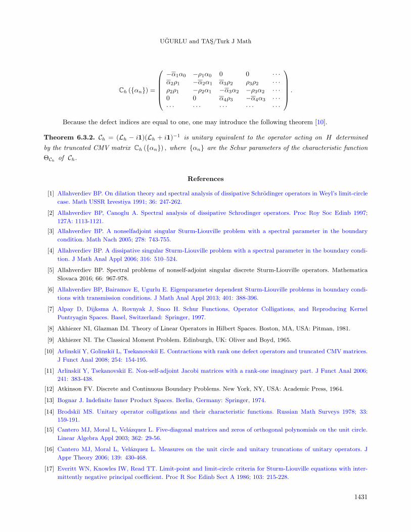
Ch (αn) =

−α1α0 −ρ1α0 0 0 · · ·α2ρ1 −α2α1 α3ρ2 ρ3ρ2 · · ·ρ2ρ1 −ρ2α1 −α3α2 −ρ3α2 · · ·0 0 α4ρ3 −α4α3 · · ·· · · · · · · · · · · · · · ·

.

Because the defect indices are equal to one, one may introduce the following theorem [10].

Theorem 6.3.2. Ch = (Lh − i1)(Lh + i1)−1 is unitary equivalent to the operator acting on H determined

by the truncated CMV matrix Ch (αn) , where αn are the Schur parameters of the characteristic function

ΘChof Ch.

References

[1] Allahverdiev BP. On dilation theory and spectral analysis of dissipative Schrodinger operators in Weyl’s limit-circle

case. Math USSR Izvestiya 1991; 36: 247-262.

[2] Allahverdiev BP, Canoglu A. Spectral analysis of dissipative Schrodinger operators. Proc Roy Soc Edinb 1997;

127A: 1113-1121.

[3] Allahverdiev BP. A nonselfadjoint singular Sturm-Liouville problem with a spectral parameter in the boundary

condition. Math Nach 2005; 278: 743-755.

[4] Allahverdiev BP. A dissipative singular Sturm-Liouville problem with a spectral parameter in the boundary condi-

tion. J Math Anal Appl 2006; 316: 510–524.

[5] Allahverdiev BP. Spectral problems of nonself-adjoint singular discrete Sturm-Liouville operators. Mathematica

Slovaca 2016; 66: 967-978.

[6] Allahverdiev BP, Bairamov E, Ugurlu E. Eigenparameter dependent Sturm-Liouville problems in boundary condi-

tions with transmission conditions. J Math Anal Appl 2013; 401: 388-396.

[7] Alpay D, Dijksma A, Rovnyak J, Snoo H. Schur Functions, Operator Colligations, and Reproducing Kernel

Pontryagin Spaces. Basel, Switzerland: Springer, 1997.

[8] Akhiezer NI, Glazman IM. Theory of Linear Operators in Hilbert Spaces. Boston, MA, USA: Pitman, 1981.

[9] Akhiezer NI. The Classical Moment Problem. Edinburgh, UK: Oliver and Boyd, 1965.

[10] Arlinskiı Y, Golinskiı L, Tsekanovskiı E. Contractions with rank one defect operators and truncated CMV matrices.

J Funct Anal 2008; 254: 154-195.

[11] Arlinskiı Y, Tsekanovskiı E. Non-self-adjoint Jacobi matrices with a rank-one imaginary part. J Funct Anal 2006;

241: 383-438.

[12] Atkinson FV. Discrete and Continuous Boundary Problems. New York, NY, USA: Academic Press, 1964.

[13] Bognar J. Indefinite Inner Product Spaces. Berlin, Germany: Springer, 1974.

[14] Brodskiı MS. Unitary operator colligations and their characteristic functions. Russian Math Surveys 1978; 33:

159-191.

[15] Cantero MJ, Moral L, Velazquez L. Five-diagonal matrices and zeros of orthogonal polynomials on the unit circle.

Linear Algebra Appl 2003; 362: 29-56.

[16] Cantero MJ, Moral L, Velazquez L. Measures on the unit circle and unitary truncations of unitary operators. J

Appr Theory 2006; 139: 430-468.

[17] Everitt WN, Knowles IW, Read TT. Limit-point and limit-circle criteria for Sturm-Liouville equations with inter-

mittently negative principal coefficient. Proc R Soc Edinb Sect A 1986; 103: 215-228.

1431

UGURLU and TAS/Turk J Math

[18] Gesztesy F, Zinchenko M. Weyl-Titchmarsh theory for CMV operators associated with orthogonal polynomials on

the unit circle. J Appr Theory 2006; 139: 172-213.

[19] Gorbachuk VI, Gorbachuk ML. Boundary Value Problems for Operator Differential Equations. Kiev, USSR:

Naukova Dumka, 1984.

[20] Harris BJ. Limit-circle criteria for second order differential expression. Quart J Math Oxford Ser (2) 1984; 35:

415-427.

[21] Kreyszig E. Introductory Functional Analysis with Applications. New2 York, NY, USA: Wiley, 1978.

[22] Maozhu Z, Sun J, Zettl A. The spectrum of singular Sturm-Liouville problems with eigenparameter dependent

boundary conditions and its approximation. Results Math 2013; 63: 1311-1330.

[23] Markus AS. The problem of spectral synthesis for operators with point spectrum. Math USSR Izvestija 1970; 4:

670-696.

[24] Nagy BSz, Foias C. Harmonic Analysis of Operators on Hilbert Space. Budapest, Hungary: Academia Kioda, 1970.

[25] Nagy BSz, Foias C, Bercovici H, Kerchy L. Harmonic Analysis of Operators on Hilbert Space. Revised and Enlarged

Edition. New York, NY, USA: Springer, 2010.

[26] Naimark MA. Linear Differential Operators. Moscow, USSR: Nauka, 1969; English transl of 1st edn New York, NY,

USA: Ungar, 1968.

[27] Nikolskiı N, Vasyunin V. Elements of spectral theory in terms of free functional model part I: basic constructions.

MSRI Publ 1998; 33: 211-302.

[28] Nikolskiı N. Operators, Functions, and Systems: An Easy Reading, vol. 2. Model Operators and Systems. Math

Surveys and Monogr 92, Amer Math Soc, Providence, RI, USA; 2002.

[29] Nikolskiı NK. Treatise on the Shift Operator. Berlin, Germany: Springer-Verlag, 1986.

[30] Pavlov BS. Dilation theory and spectral analysis of nonselfadjoint differential operators. Math Programming and

Related Questions (Proc. Seventh Winter School, Drogobych, 1974): Theory of Operators in Linear Spaces, Tsentral

Ekonom-Mat. Inst Akad Nauk, Moscow, SSSR: 1976, pp. 3-69.

[31] Pavlov BS. Spectral analysis of a dissipative singular Schr odinger operator in terms of a functional model. Itogi

Nauki Tekh Ser Sovrem Probl Math Fundam Napravleniya 1991; 65: 95-163.

[32] Sarason D. On spectral sets having connected complement. Acta Sci Math 1965; 26: 289-299 (Szeged).

[33] Simon B. CMV matrices: Five years after. J Comput Appl Math 2007; 208: 120-154.

[34] Simon B. Analogs of the m− function in the theory of orthogonal polynomials on the unit circle. J Comput Appl

Math 2004; 171: 411-424.

[35] Solomyak BM. Functional model for dissipative operators. A coordinate-free approach. J Soviet Math 1992; 61:

1981-2002.

[36] Ugurlu E, Bairamov E. Spectral analysis of eigenparameter dependent boundary value transmission problems. J

Math Anal Appl 2014; 413: 482-494.

[37] Wang Z, Wu H. Dissipative non-self-adjoint Sturm-Liouville operators and completeness of their eigenfunctions. J

Math Anal Appl 2012; 394: 1-12.

[38] Zettl A. Sturm-Liouville Theory. Mathematical Surveys and Monographs 121. American Mathematical Society,

Providence, RI, USA; 2005.

1432