NAVAL POSTGRADUATE SCHOOL Monterey, California

DISSERTATION

NEARSHORE WAVE AND CURRENT DYNAMICS

by

Bruce J. Morris

September 2001

Dissertation Advisor: Edward B. Thornton Committee Members: Thomas H.C. Herbers Timothy P. Stanton Adrianus J.H.M. Reniers Kenneth L. Davidson

Approved for public release; distribution is unlimited

Report Documentation Page

Report Date 30 Sep 2001

Report Type N/A

Dates Covered (from... to) -

Title and Subtitle Nearshore Wave and Current Dynamics

Contract Number

Grant Number

Program Element Number

Author(s) Morris, Bruce J.

Project Number

Task Number

Work Unit Number

Performing Organization Name(s) and Address(es) Research Office Naval Postgraduate School Monterey,Ca 93943-5138

Performing Organization Report Number

Sponsoring/Monitoring Agency Name(s) and Address(es)

Sponsor/Monitor’s Acronym(s)

Sponsor/Monitor’s Report Number(s)

Distribution/Availability Statement Approved for public release, distribution unlimited

Supplementary Notes

Abstract

Subject Terms

Report Classification unclassified

Classification of this page unclassified

Classification of Abstract unclassified

Limitation of Abstract UU

Number of Pages 100

REPORT DOCUMENTATION PAGE Form Approved OMB No. 0704-0188 Public reporting burden for this collection of information is estimated to average 1 hour per response, including the time for reviewing instruction, searching existing data sources, gathering and maintaining the data needed, and completing and reviewing the collection of information. Send comments regarding this burden estimate or any other aspect of this collection of information, including suggestions for reducing this burden, to Washington headquarters Services, Directorate for Information Operations and Reports, 1215 Jefferson Davis Highway, Suite 1204, Arlington, VA 22202-4302, and to the Office of Management and Budget, Paperwork Reduction Project (0704-0188) Washington DC 20503. 1. AGENCY USE ONLY (Leave blank)

2. REPORT DATE Month Year

September 2001

3. REPORT TYPE AND DATES COVERED Doctoral Dissertation

4. TITLE AND SUBTITLE: Nearshore Wave and Current Dynamics

6. AUTHOR(S) Morris, Bruce J..

5. FUNDING NUMBERS N0001401WR20023

7. PERFORMING ORGANIZATION NAME(S) AND ADDRESS(ES) Naval Postgraduate School Monterey, CA 93943-5000

8. PERFORMING ORGANIZATION REPORT NUMBER

9. SPONSORING / MONITORING AGENCY NAME(S) AND ADDRESS(ES) N/A

10. SPONSORING / MONITORING AGENCY REPORT NUMBER

11. SUPPLEMENTARY NOTES The views expressed in this thesis are those of the author and do not reflect the official policy or position of the Department of Defense or the U.S. Government. 12a. DISTRIBUTION / AVAILABILITY STATEMENT Approved for public release; distribution is unlimited.

12b. DISTRIBUTION CODE

13. ABSTRACT (maximum 200 words) Mean cross-shore wave height transformation and alongshore currents observed on near-planar and barred beaches are compared with predictions based on the nearshore numerical model Delft3D. Delft3D solves the two-dimensional, depth-averaged, alongshore momentum balance between forcing (by breaking waves and variations in mean surface elevation), changes in momentum flux, bottom stress and lateral mixing. The observations were acquired on the near-planar California beaches at Torrey Pines and Santa Barbara and the barred beach at Duck, N.C., and include a wide range of conditions with maximum mean currents of 1.5 m/s. The model has two free parameters, a depth dependent breaking term, γ , and the bed

roughness length, sk . An empirical formula to determine γ a priori from the deep water wave steepness and bed slope is developed, showing good agreement in the wave height transformation. Including rollers in the wave forcing results in improved predictions of the observed alongshore current structure by shifting the predicted velocity maxima shoreward and increasing the velocity in the trough of the bar compared with model predictions without rollers. On near-planar beaches and high-energy events on barred beaches, a 1-D (alongshore uniform bathymetry) model performs as well as 2-DH. On barred beaches under moderate conditions when alongshore non-uniform bathymetry prevails, the 2-DH model performs better than the 1-D model, particularly in the bar-trough region. Wave forcing balances the bottom stress with a second balance between alongshore variation in the mean surface elevation (pressure gradients) and the inertia of the alongshore current.

15. NUMBER OF PAGES

89

14. SUBJECT TERMS alongshore current, nearshore momentum balance, Delft3D, barred beach, planar beach, rollers.

16. PRICE CODE

17. SECURITY CLASSIFICATION OF REPORT

Unclassified

18. SECURITY CLASSIFICATION OF THIS PAGE

Unclassified

19. SECURITY CLASSIFICATION OF ABSTRACT

Unclassified

20. LIMITATION OF ABSTRACT

UL

NSN 7540-01-280-5500 Standard Form 298 (Rev. 2-89) Prescribed by ANSI Std. 239-18

i

THIS PAGE INTENTIONALLY LEFT BLANK

ii

Approved for public release; distribution is unlimited

NEARSHORE WAVE AND CURRENT DYNAMICS

Bruce J. Morris Lieutenant Commander, United States Navy B.S., United States Naval Academy, 1988

M.S., Naval Postgraduate School, 1997

Submitted in partial fulfillment of the requirements for the degree of

DOCTOR OF PHILOSOPHY IN PHYSICAL OCEANOGRAPHY

from the

Author:

Approved by:

NAVAL POSTGRADUATE SCHOOL September 2001

Bruce J. Morris

Edward B. Thornton Distinguished Professor of Oceanography Dissertation Supervisor

Timothy P. Stanton Research Associate Professor of Oceanography

Kenneth L. Davidson Professor of Meteorology

Thomas H. C. Herbers Associate Professor of Oceanography

/^Adrianus J. H. M. Reniers ^-MIC Fellow

Approved by: ^m^ ^a%&. Mary L. Batteen, Chair, Department of Oceanography

Approved by: \^/AA^\ j Q^^^^s Carson K. Eoyang, Associate Probst for Academic Affairs

in

THIS PAGE INTENTIONALLY LEFT BLANK

iv

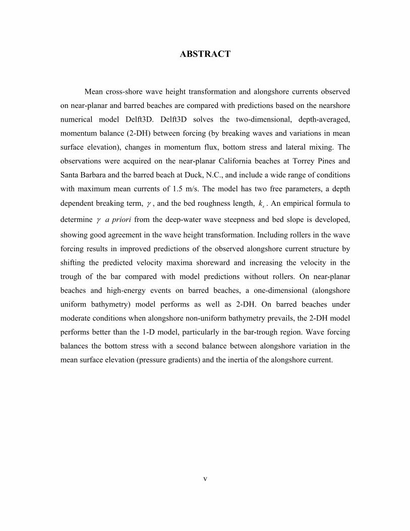
ABSTRACT Mean cross-shore wave height transformation and alongshore currents observed

on near-planar and barred beaches are compared with predictions based on the nearshore

numerical model Delft3D. Delft3D solves the two-dimensional, depth-averaged,

momentum balance (2-DH) between forcing (by breaking waves and variations in mean

surface elevation), changes in momentum flux, bottom stress and lateral mixing. The

observations were acquired on the near-planar California beaches at Torrey Pines and

Santa Barbara and the barred beach at Duck, N.C., and include a wide range of conditions

with maximum mean currents of 1.5 m/s. The model has two free parameters, a depth

dependent breaking term, γ , and the bed roughness length, sk . An empirical formula to

determine γ a priori from the deep-water wave steepness and bed slope is developed,

showing good agreement in the wave height transformation. Including rollers in the wave

forcing results in improved predictions of the observed alongshore current structure by

shifting the predicted velocity maxima shoreward and increasing the velocity in the

trough of the bar compared with model predictions without rollers. On near-planar

beaches and high-energy events on barred beaches, a one-dimensional (alongshore

uniform bathymetry) model performs as well as 2-DH. On barred beaches under

moderate conditions when alongshore non-uniform bathymetry prevails, the 2-DH model

performs better than the 1-D model, particularly in the bar-trough region. Wave forcing

balances the bottom stress with a second balance between alongshore variation in the

mean surface elevation (pressure gradients) and the inertia of the alongshore current.

v

THIS PAGE INTENTIONALLY LEFT BLANK

vi

TABLE OF CONTENTS

I. INTRODUCTION........................................................................................................1 A. MOTIVATION ................................................................................................1 B. OBJECTIVES ..................................................................................................3

II. MODEL EQUATIONS ...............................................................................................5 A. DELFT3D EQUATIONS (NO ROLLER)....................................................5

1. Wave Model..........................................................................................5 2. Flow Model ...........................................................................................6

B. DELFT3D EQUATIONS (ROLLER)............................................................7 1. Wave Model..........................................................................................7 2. Flow Model ...........................................................................................8

C. MODEL FORMULATION.............................................................................8

III. FIELD DATA.............................................................................................................11 A. PLANAR BEACH..........................................................................................11

1. Torrey pines........................................................................................11 2. Santa Barbara ....................................................................................11

B. BARRED BEACH .........................................................................................12 1. Delilah .................................................................................................12 2. Duck94 ................................................................................................13

IV. MODEL RESULTS ...................................................................................................15 A. MODEL-DATA COMPARISON TECHNIQUES .....................................15 B. MODEL PARAMETERS .............................................................................16

1. Wave Breaking Parameter ( )γ ........................................................16 a. Introduction.............................................................................16 b. Observations ............................................................................16 c. Model-Data Comparison.........................................................17

2. Bed Roughness Length ( )sk ..............................................................20 a. Best-fit Values .........................................................................20 b. Observations ............................................................................21 c. Model-Data Comparisons .......................................................22 d. Summary..................................................................................24

C. 1-DH VERSUS 2-DH MODELING .............................................................25 1. Introduction........................................................................................25 2. Barred Beach......................................................................................26

a. Introduction.............................................................................26 b. Cross-shore Variation of rmsH ...............................................27 c. Cross-shore Variation of xv ...................................................28 d. Alongshore Variation of yv ....................................................31

vii3. Planar Beach.......................................................................................32

a. Introduction.............................................................................32 b. Cross-shore Variation of and rmsH xv ...................................32

4. Summary.............................................................................................33 D. MOMENTUM ANALYSIS (BARRED BEACH).......................................34

1. Uniform vs Measured Bathymetry...................................................34 2. Alongshore Variation of the Total Momentum...............................37

E. MOMENTUM ANALYSIS (PLANAR BEACH) .......................................39 1. Model vs. Measured Results..............................................................39 2. Alongshore Variation of the Total Momentum...............................39

V. SUMMARY AND CONCLUSIONS ........................................................................41

LIST OF REFERENCES......................................................................................................85

INITIAL DISTRIBUTION LIST .........................................................................................89

viii

ACKNOWLEDGMENTS First, I wish to express my deep appreciation to Distinguished Professor Ed

Thornton, not only for his dedication and assistance as my dissertation supervisor, but

more so for his fatherly advice and mentorship.

Secondly, thanks to the rest of my committee: Professors Tom Herbers, Ken

Davidson, Tim Stanton and Dr. Ad Reniers for their advice and guidance. Ad a special

thanks for your patience and time in explaining and re-explaining nearshore concepts to

me.

I also wish to express my gratitude to the fine personel of the NPS Oceanography

Department and METOC Curricular Office for their help throughout the project;

particularly Mr. Mark Orzech for generously sharing his insight into computer

programming and Mrs. Eva Anderson for her excellent administrative support.

Most importantly I wish to thank my family, Petra, Colton, Victoria, Elizabeth

and Claire. Without whose support, encouragement and understanding, I would certainly

not have been able to finish this dissertation.

ix

THIS PAGE INTENTIONALLY LEFT BLANK

x

I. INTRODUCTION

A. MOTIVATION

On planar beaches, as depth decreases, waves shoal then break and, depending on

the slope of the beach, create a narrow to broad cross-shore distribution of breaking

waves known as the surf zone. On barred beaches, waves break over the bar, reform in

the trough and break again on the shore. Resulting nearshore currents generated by

obliquely incident breaking waves within the surf zone can exceed 1 during times of

large incident angle or high wave conditions. Thus, the modeling of nearshore circulation

assumes a special significance for military operations, where the success or failure of an

amphibious operation or infiltration/exfiltration of Special Forces is directly related to

our ability to forecast the conditions within this dynamic area.

m s

Nearshore flow modeling often assumes alongshore uniformity in the bathymetry.

This simplifies the momentum equations to 1-D in the cross-shore resulting in a

mathematical balance between the wave forcing and bottom friction in the alongshore

and the wave forcing and cross-shore pressure gradient in the cross-shore direction

(Bowen (1969), Longuet Higgins (1970) and Thornton (1970)). Verifying this

assumption using a 1-D model in conjunction with field data proves surprisingly accurate

for near-planar beaches (Thornton and Guza, 1986). However on barred beaches, the 1-D

assumption has proved less successful when compared with measured data, especially

under mild wave conditions (Church and Thornton, 1993 and Smith et al., 1993).

Random wave 1-D models that assume wave energy dissipation occurs locally at wave

breaking (Battjes and Janssen, 1978; Thornton and Guza, 1983) result in local radiation

stress gradients and alongshore currents predicted over the bar and at the shore. However,

the alongshore current profiles obtained during the Delilah field experiment at the U.S.

Army Corp of Engineers Field Research Facility (FRF) Duck, NC show that most of the

time the current maximum was within the trough and not at locations where intense wave

breaking occurred.

Varying hypotheses have been put forth to explain why the current maximum

occurred over the trough. These include rollers (turbulent layer riding on the forward face

1

of the wave crest) during breaking, alongshore pressure gradients and mixing of

momentum by various mechanisms. Svendson (1984) introduced the concept of a surface

roller that allows wave energy to be transferred to a roller prior to dissipating. The time

required for the roller to dissipate the energy creates a spatial lag between wave breaking

and the energy dissipation (Nairn et al., 1990). Comparisons of 1-D roller models with

both lab (Reniers and Battjes, 1997) and field data (Lippmann, Brookins and Thornton,

1996) have shown the effect of the roller is to shift the wave energy dissipation

shoreward. The roller dissipation mechanism has resulted in an improvement in the cross-

shore profile of the alongshore current on barred beaches, but does not completely

account for the current maxima residing in the trough.

Since most beaches fail to maintain alongshore uniformity in their bathymetry for

any length of time, assuming alongshore uniformity can prove to be too simplistic.

Therefore, in general, the full horizontal two-dimensional depth-averaged (2-DH)

equations should be used to compute the spatial distribution of the wave and flow field.

Putrevu et al., (1995) showed analytically that small alongshore variations in bottom

topography can induce alongshore pressure gradients caused by alongshore gradients in

breaking wave height and concomitant set-up that can force an alongshore current in the

trough. Sancho et al., (1995) used a quasi-3D model with no roller dissipation over

smoothed bathymetry simulating a barred beach (Duck94) to examine contributions of

the different terms in the momentum equations to the flow field. They found that the

pressure gradient plays a significant role in the alongshore flow pattern, resulting in

single-peak alongshore current profiles. Slinn et al., (2000) also examined contribution to

the momentum equations using a 2-DH depth averaged model with no roller dissipation

over smoothed sinuous bathymetry designed to approximate a barred beach from the

Delilah experiment. Again a correlation was found between the pressure gradient and

flow field structure. Neither compared wave and current model output with measured

data from the beaches they were simulating.

2

Currently the U.S. Navy utilizes the Navy Standard Surfzone Model (NSSM),

which provides predicted wave heights and mean currents across the surf zone. The

present surf model is limited by simplified hydrodynamics (1-D) and the assumption of

alongshore uniform bathymetry. Depth-averaged (2-DH) nearshore numerical models,

which allow for the inclusion of measured bathymetry and complete physics in the cross-

shore and alongshore momentum equations, have been in development in Europe over

the past two decades under the Marine and Science Technology (MAST) program. A

number of mature models have evolved including those by Delft Hydraulics (Delft3D),

Danish Hydraulic Institute, Service Technique Central des Ports Maritimes et des Voies

Navigables, HR Wallingford, Civil Engineering Department of the University of

Liverpool (Nicholson et al., 1997) and the University of Delaware. Model differences

reside in the content of the wave driver and hydrodynamics. Wave drivers vary by linear

or non-linear monochromatic or random waves, wave diffraction and wave friction.

Horizontal circulation models solve the depth-averaged Navier-Stokes equations using

eddy viscosity turbulence closure, but differ in their evaluation of eddy viscosity using

either a constant or allowing spatially variability. Bottom friction in the current models is

characterized either as a parameterization of bed shear stress utilizing wave-current

interaction or separately by wave or current forcing. The Naval Postgraduate School,

Department of Oceanography, Nearshore Group was funded by the Office of Naval

Research to assess the Delft3D model as an upgrade to the Navy Standard Surf Model.

B. OBJECTIVES

The objectives of this dissertation are to assess and improve the ability to forecast

wave and hydrodynamic conditions in the nearshore through the evaluation and

improvement of the nearshore model Delft3D. Delft3D is an improvement over NSSM in

that it includes the use of non-uniform bathymetry, an improved wave driver and the

depth averaged 2-DH momentum equations. Assessment of the robustness and accuracy

of the model is made by comparing it with existing field data from both near-planar and

barred beaches, investigating the gains realized by advancing from 1-D to 2-DH

hydrodynamics with 3-D bathymetry and assessing the implementation of a roller wave

dissipation mechanism. Once the prediction skill of the Delft3D model is established, the

focus is to improve our understanding of the contributions of the terms in the cross-shore

and alongshore momentum equations to the nearshore flow field.

3

The work is organized as follows: Model equations, sensitivity of the model to the

free parameters and the model formulation are presented in Chapter II. Chapter III

discusses beach types, instrument layout and wave/current conditions during the

experiments conducted at Torrey Pines and Santa Barbara, California and Duck, North

Carolina. The 1-D versus 2-DH model experiments of the contributions of the momentum

terms to the flow field are presented in Chapter IV. Conclusions and recommendations

are presented in Chapter V.

4

II. MODEL EQUATIONS

A. DELFT3D EQUATIONS (NO ROLLER)

1. Wave Model

Assuming steady state conditions, no mean current, no wind forcing and initial

offshore waves described in terms of a Raleigh wave height distribution, a 2-D version of

Battjes and Janssen (1978) wave transformation model is used to solve the wave energy

balance as described by HISWA (Holthuijsen et al., 1989) with local energy dissipation

described as a linear bore

( ) ( ) ( )2max 0

0 0 0 8b

g g g wx ytot

Q fH EE C E C E C D Bx y θθ π∂ ∂ ∂

+ + = − = −∂ ∂ ∂ E

(1)

where is a function of wave direction and parameterized as a frequency spectrum of

fixed shape,

0E

g xC and g y

C represent rectilinear propagation, gCθ represents refraction, B

is a coefficient of O(1), f the average frequency, is the depth limited wave height

and is proportional to the wave energy integrated over all directions. The

fraction of breaking waves, Q , is assumed to occur as a delta function at in

a truncated Raleigh distribution which results in the implicit relation

maxH

2rmsHtotE =

b maxrmsH H=

(2) ( )( ) 2

max

18

lnb tot

b

Q EQ H

−= −

where is the maximum wave height given by maxH

=

88.0tanh88.0

maxkh

kH γ (3)

in which k is the wave number corresponding to pf . In shallow water, the coefficientγ

represents the ratio of the breaking wave height to water depth, h, and is the only

unknown coefficient in the model. The input to the model is the measured bathymetry

and measured wave conditions offshore. The measured wave conditions include the

5

significant wave height, peak wave period, mean incident wave angle and the directional

spread.

ji,

κ

2. Flow Model

The flow module solves the depth averaged, non-steady, x- and y- momentum

equations given by

2 1, 21 ;1,2

jii ij i

j i j

S iu uu g ujt x x h x τ

η υ τρ ∂ =∂ ∂ ∂

+ = − − + ∇ − =∂ ∂ ∂ ∂ i (4)

where refer to horizontal components x , , u the depth-averaged velocity, y i η

represents the surface elevation, and iτ the combined wave and current bottom shear

stress in the cross-shore and alongshore direction. The radiation stresses in both the cross-

shore and alongshore are not solved directly, but formulated as proportional to the

dissipation divided by the wave celerity (Dingemans et al., 1987)

(5) i

w

j

ji kD

xS

ω≈

∂

∂

which is exact in the alongshore but approximate in the cross-shore. This approximation

prevents spurious currents from forming in the flow field. The eddy viscosity, τυ ,

associated with lateral mixing is held constant at 0.1 sm2 . The bottom shear stress is

computed using Soulsby et al., (1993) linearized summation of combined wave and

current stresses

( )i c wτ κ τ τ= +

where is a fitting function of the Fredsoe (1984) non-linear stress model. The

shear stress due to the current is calculated using a quadratic formulation, c fcτ ρ=

where U is the mean current. The bed shear stress coefficient is described after W

Colebrook

2

101218log

f

s

gch

k

=

6

(6)

bed 2

U ,

hite-

(7)

where the Nikuradse roughness length, , typically related to grain size, is used as the

fitting parameter for the circulation portion of the model. The bed stress due to the waves

is modeled as with being the wave friction factor and U the

amplitude of the near-bottom wave orbital velocity in the direction of wave propagation

based on the .

sk

wf2ˆ5.0 orbww Ufρτ =

rms

orbˆ

H

B. DELFT3D EQUATIONS (ROLLER)

1. Wave Model

The inclusion of the roller dissipation mechanism requires modification to the

wave transformation model (Reniers, 1999). The balance for the short wave energy, ,

to describe the propagation of the short wave groups on variable bathymetry is given by

wE

(8) cos( ) sin( )w g w g

w

E C E CD

x yθ θ∂ ∂

+ = −∂ ∂

where θ is the angle of incidence with respect to the x-axis, x the cross-shore distance

and the alongshore distance. y gC and θ are obtained from the pre-computed wave

refraction over the bottom bathymetry utilizing HISWA. The wave energy dissipation,

, serves as input in the balance for the roller energy balance wD

(9) wr

rr DDy

cEx

cE+−=

∂∂

+∂

∂ )sin(2)cos(2 θθ

where is the roller energy, c the phase speed, rE tr cD τ= represents the roller energy

dissipation expressed by (Deigaard, 1993) and tτ represents the wave-averaged shear

stress between the roller and the wave interface. The shear stress for a steady roller is

given by (Duncan, 1981)

(10)L

gAt

)sin(βρτ =

where ρ is the water density, g is gravitational acceleration, β represents the slope of

the wave front, is the roller area and is the wave length corresponding to the peak

period. Roller energy area is related to the roller energy by (Svendsen, 1984)

A L

(11) 7

LcAEr 2

2ρ=

combining equations (2) and (3) using the roller energy dissipation results in

(12) c

EgD rr

)sin(2 β=

with β an additional free parameter, held constant at 0.04 throughout the assessment,

consistent with values found by Walstra et al., 1996. In general, advection length of the

roller increases with decreasing β . , is taken to be zero at the upwave boundaries. rE

2. Flow Model

The momentum equations with the roller included differ in two ways. First, the

radiation stress terms include a roller contribution (Reniers, 1999)

(13) 2

1, 22 2 1 ;

1, 22g i j gw

ij w r ij

C k k C iES E Ejc k c

δ=

= + + − =

where is the wave energy, wE 2i jk k k are the direction cosines in both the cross-shore

and alongshore, is the wave number, c is the phase speed, C is group velocity and the

eddy viscosity. Secondly, eddy viscosity coefficient

k g

tυ , associated with lateral mixing is

determined using a formulation by Battjes (1975)

31

=

ρυ r

tDh

(14)

where the roller energy dissipation, , is obtained from the roller transformation.

Hereafter, the combined eddy viscosity and eddy viscosity coefficient are termed

turbulent mixing ( ).

rD

tm

C. MODEL FORMULATION

The numerical model is described in detail by Stelling (1984) and Verboom and

Slob (1984). It is a finite difference model utilizing an Alternating Direction Implicit

(ADI) technique on a staggered grid. The ADI scheme implicitly solves the water levels

and velocities in the x -direction in the first half of the time step and the directed terms y8

in the second. The grid spacing is varied based on the bathymetry feature needing to be

resolved. In general, 10 grid points are needed to capture the feature of interest. For

Delilah a grid spacing of x∆ =3 m, y∆ =6 m is used to capture the non-uniform

bathymetry in the cross-shore and alongshore. For Santa Barbara and Torrey Pines a finer

resolution was required ( x∆ =1 m, y∆ =2) due to the steepness of the beach in the cross-

shore and the longer period incident swells. The time step utilized ( t∆ = 1.5 s) is based

on the Courant number, CFL, for wave propagation

CFL t gh= <2 2

1 12 1x y

∆ + ∆ ∆ 0 (15)

where x∆ and are the smallest grid spaces in the physical space. y∆

Model bathymetry is created from bathymetry measurements taken during the

various field experiments using a triangular interpolation scheme. The criteria for

offshore boundary location consists of minimizing the number of grid points required to

fill the domain of interest and selecting a water depth well outside wave breaking. This

resulted in an offshore boundary water depth of 4 m. for all days examined except the

large wave days at Delilah (Oct. 11-13) where wave shoaling at = 4 m required the

boundaries be moved to 8 m. The daily bathymetry collected during Delilah extended to

approximately 4 m depth with a pre and post experiment extension to 8 m. In order to

develop model bathymetry to 8 m, a composite of the daily measured bathymetry was

merged with the post experiment 8 m set. This proved adequate as the bathymetry from 4

m depth to 8 m changed little between the pre and post 8 m bathymetry set. A smoothing

scheme is implemented over the model bathymetry for days when the bar was attached to

the shore (Delilah: Oct. 7-9) to prevent large alongshore depth gradients from causing

unrealistic flow patterns.

h

The boundary conditions for the wave model are separated into those required to

satisfy the HISWA wave model (Equation 1) and those for the wave model using a roller

dissipation mechanism (Equations 8 and 9). The HISWA offshore boundary requires

input of the significant wave height, incident wave angle, peak wave period and

directional spreading. Values for the offshore boundary wave input are derived from the

8m arrays and linearly shoaled and refracted to the 4 m water depth. The wave energy at

9

the lateral boundaries was chosen to be zero. In the case of the wave model that included

a roller dissipation mechanism, the roller energy is prescribed zero at the offshore and

lateral boundaries.

In addition to prescribing tidal elevation at the boundaries, the flow model

requires two boundary conditions for closure at the offshore and lateral boundaries. First

a Riemann invariant is used to allow disturbances, created by differences in water

elevation between the boundary and inner domain, traveling perpendicular to the

boundaries to pass in a non-reflective manner. The second flow boundary condition is

such that at inflow the advection of momentum in the tangential direction is neglected. At

the land-water interface it is assumed no flow through the boundary and zero tangential

shear stress (free slip).

Steep incident wave angles O(20°) can result in large setup gradients near the

lateral boundaries close to shore resulting in unrealistic circulations and flow forcing that

can propagate into the model domain. To prevent boundary generated disturbances from

contaminating the flow field, the model domain is extended in the alongshore O(500) m

on either side of the domain area of interest. The extension is created with a systematic

increase in alongshore grid spacing, culminating in a y∆ of 50 m at the lateral

boundaries. These large grid steps act to diffuse the water level gradients and prevent

spurious currents from propagating into the domain. The bathymetry in this portion of the

grid is expanded uniformly alongshore from the last measured cross-shore profile prior to

the artificial extension.

10

III. FIELD DATA

A. PLANAR BEACH

1. Torrey pines

The Torrey Pines Beach, located north of San Diego, California, is near-planar

with a gentle (1:50) slope. Due to shadowing and refraction by offshore islands, the

incident swell direction was less than 15 deg. One-hour records were analyzed for data

acquired on Nov. 10,14,18,20-21, 1978 (17 hours). The peak frequency of the incident

wave spectra varied little during the experiment and was about 0.06-0.08 Hz (T = 12.5-

16 s). The rms wave height ranged between 0.47 – 0.69 m in 8 m depth and initial

offshore rms wave height (in the model) was set equal to the measured hourly value.

During this experiment and all other experiments described herein the cross-shore

transect of wave heights and currents were measured using a cross-shore array of

pressure sensors and Marsh-McBirney electromagnetic current meters. The pressure array

extended from 8 meters depth to inside the surf zone with the current meter array from

2.5 meters depth to inside the surf zone (Thornton and Guza, 1983). The data were

sampled at 2 Hz. The tidal range is 2 m. Only data over the high tide are used when

instruments are submerged. Surface elevations are inferred from pressure data for all data

sets described herein by applying the appropriate linear wave theory spectral

transformation (Guza and Thornton, 1980). The data are band-pass filtered from 0.05 to

0.3 Hz to remove high frequency noise and low frequency (surfbeat) waves.

p

8Hrms ησ=

is calculated, where 2ησ is the surface elevation variance. Bathymetry profiles were

collected daily by rod and level survey along the measurement transect. Table 4.1

summarizes wave conditions and bottom slopes for the beaches analyzed.

2. Santa Barbara

Leadbetter Beach located in Santa Barbara, California is a mild (1:25) sloping

near-planar beach with a tidal range of 2 m. Protection by the offshore Channel Islands

11

and Point Conception to the north results in a narrow aperture for incoming ocean swell

(less than 9 deg). Pressure and velocity data were acquired at 14 locations in a cross-

shore array starting in 3 meters (Thornton and Guza, 1986). Data were sampled at 2 Hz.

The measurements were taken over high tide when all instruments were submerged. The

3 days of data (Feb. 4-6: 13 hours) utilized for model comparison consist of narrow-

banded incident waves with periods ranging between 12.0-14.3 s and relatively small

wave heights ( = 0.29-0.65 m). Daily nearshore bathymetry profiles were measured

by rod and level surveys at 5 cross-shore range lines covering an alongshore extent of

200 meters.

rmsH

B. BARRED BEACH

1. Delilah

The beach at Duck, North Carolina is typically a barred beach with a mean tidal

range of approximately 1 m. The mean foreshore slope of the beach is approximately

0.08 (1:12) and 1:35 offshore from the bar. Wave heights during the Delilah experiment

were measured using a cross-shore array of 9 pressure sensors. The data were sampled at

8 Hz continuously from Oct. 7-19 (300 hours). The area of the beach where the

instruments were deployed, known as the mini-grid region, was surveyed daily along 20

cross-shore profile lines spaced 25 m apart near the instruments and 50 m apart elsewhere

resulting in an area approximately 550 m in the alongshore and 300 m in the cross-shore

to a depth of 4 m. Offshore directional wave spectra were measured using a linear

alongshore array of 10 pressure sensors in 8m depth (Long, 1994).

The waves and resulting alongshore currents varied considerably during the

experiment, Oct.1-20. Waves and currents were mild from Oct. 7-8. On Oct. 9 a strong

frontal system from the south generated broadband waves at relatively large angles (~40

degrees from the south in 8 m depth) resulting in a strong alongshore current to the north

(1.5 m/s). The wave event began to subside on the afternoon of the 11th, but on the

evening of the 12th large swell waves began to arrive from the south due to distant

Hurricane Lilli; these waves grew to a maximum on the morning of the 13th (Hs~2.5m)

then gradually diminished to a wave height of ~1m on the morning of the 14th. Although

12

the wave heights diminished, the alongshore currents remained strong (> 1m/s) for the

remainder of the experiment. Wave directions changed considerably the last 4 days with

the incident wave direction swinging from south to north and then south again on the 16th

causing the alongshore currents to change direction. The swell became bi-modal on the

17th, persisting through the 18th with the alongshore current flowing to the north. On the

19th, a small frontal system passed to the north generating waves from the north and

currents to the south.

2. Duck94

The Duck94 nearshore experiment was conducted during Sept. and Oct. 1994 at

the Field Research Facility; Duck, North Carolina. The beach during the experiment

could be characterized as a barred beach (30-120 m offshore). Directional wave spectra

were again acquired using a linear array of 10 pressure sensors in 8 m depth.

Additionally, a 13 element cross-shore array of pressure sensors was used to measure

wave heights spanning the width of the surf zone to 8 m depth. The data were sampled at

2 Hz (Elgar et al., 1997)

The data selected for analysis are from a 24-hour data run acquired on September

16th. The 16th was a mild day ( = 0.28-0.33 m) with a long period swell (T s).

This combination of conditions resulted in wave steepness values less than 0.002. Wave

data with steepness values less than 0.002 was required in the development of an

empirical formula for determining the wave breaking free parameter,

rmsH 13.7p =

γ , a priori.

13

THIS PAGE INTENTIONALLY LEFT BLANK

14

IV. MODEL RESULTS

A. MODEL-DATA COMPARISON TECHNIQUES

Comparison is made between the measured and computed results of both the

cross-shore transformation of the root mean square ( ) wave height, , and the

mean cross-shore (

rms rmsH

xv ) and alongshore ( yv ) variation of the alongshore current to

determine model performance. Model-data comparisons are evaluated by first calculating

the relative errors defined by rms

(16) ( )

( )

2

( ) ( )

2

( )

rms Model rms Measured

rms

rms Measured

P O

Oε

−=

where denotes average over all values, P is model prediction and O is the observed

quantity. The rmsε value is then subtracted from one, generating a model skill,

1 rmsskill ε= − . Skill value represents an rms difference between model predictions and

observations normalized by a known result, with a value of 0 indicating the model has no

skill, and the value 1 indicating there is no difference between model and measured data.

The statistic is not well behaved for low forcing conditions, which have maximum

observed xv and yv along an instrument transect 0.2 m s≤ . Observations for that

transect are disregarded during that hour. The model skill aids in quantifying model

performance and is used to determine optimal γ and during model calibration. In

addition, when comparing large amounts of observed and computed data, a linear

correlation, r and absolute difference,

sk

rms ε , are used

( )2

( ) ( )rms Model rms MeasuredP Oε = −

Absolute difference is not affected by small observed data values, and provides a

quantitative value for the disparity between the observations and computed results.

15

(17)

mean

B. MODEL PARAMETERS

1. Wave Breaking Parameter ( )γ

a. Introduction

The objectives of this section are to determine model sensitivity to the

depth dependent wave breaking free parameter γ , investigate an existing empirical

formulation for the determination of γ a priori, and to develop a new formulation that

expands the predictive range of γ to more beach types.

Several surf zone wave transformation models take into account random

waves and describe breaking as a linear bore with a local probability of wave breaking

function (Battjes and Janssen, 1978, Thornton and Guza, 1983). Verification of the

Battjes and Janssen random wave-breaking model was conducted by Battjes and Stive

(1985) (hereafter denoted BS85) using both laboratory and field data. They determined

an empirical formula for the single wave breaking parameter in their transformation

model

85 00.5 0.4 tanh(33 )BS sγ = +

where the deepwater wave steepness, prms LH 00 0s = , with being the deepwater

root mean square wave height and

0rmsH

20 2 pp fgL π= , the wavelength at the peak

frequency, pf . The data used by BS85 (see Figure 4.1), produced no values for less

than 0.01, a region typically associated with longer period swell.

0s

(18)

b. Observations

Wave data acquired on the near-planar California beaches at Torrey Pines

(1:50 slope) and Santa Barbara (1:25 slope) as part of the Nearshore Sediment Transport

Study (NSTS) experiments and the barred beach at Duck, NC during the Delilah (Oct.

1990) and Duck94 (Sept.-Oct. 1994) field experiments conducted at the U.S. Army Corps

of Engineers Field Research Facility (FRF) are used to expand the work of Battjes and

Stive (1985). A 2-DH version of the wave model and longer period swell with wave

steepness values ranging from 0.0009-0.02 are used to extend the BS85 calibration

16

formula for γ . These data, dominated by long period swell, resulted in an extensive

range of values less than 0.01 (a region not yet evaluated for empirical dependence of 0s

γ on ) to include data with values less than 0.002 (a region where 0s 0s γ becomes

independent of ), Figure 4.1. 0s

c. Model-Data Comparison

The wave model was run to optimize the wave breaking parameter, optγ ,

based on iteratively minimizing the relative error, rmsε , (Equation 16) between

measurements and the model predicted along the cross-shore transect, under the

constraint

rmsH

B =1. The best fit values for the wave breaking parameter, optγ , are determined

using one hour means from the 354 hours of observed data acquired during the

Torrey Pines (17 hours), Santa Barbara (13 hours), Delilah (300 hours) and Duck94 (24

hours) experiments. Waves measured offshore during the one-hour observation are used

as input to the wave model. The resultant model output values are compared with

measured data from the various beach types with differences between the computed and

measured compared statistically.

rmsH

rmsH

rmsH

The 85BSγ values are determined using the empirical formula, Equation 18

using the same 350 hours of data. Values for are derived from the deep water wave

height determined by reverse shoaling and refracting measured from the farthest

off-shore pressure sensor (indicated with the subscript , Equation 19) in the cross-shore

transect, assuming a plane sloping bed offshore and using linear wave theory

transformation at the peak period,

0s

rmsH

r

(19)0

1 12 2

0 0

coscosr

gr rrms rms

g

CH H

Cθθ

=

where subscript indicates deepwater, 0 gC represents the group speed and θ is the mean

incident wave angle.

17

As typical examples, model predictions are compared as a function

of cross-shore distance with measured values (*) from Torrey Pines, Santa Barbara,

Delilah and Duck94 (Figure 4.2). The bottom profile is given as a reference. Model

results are shown for both

rmsH

optγ (solid line) and 85BSγ (dashed line) with skill value

included (legend box, Figure 4.2). Both the Torrey Pines and Santa Barbara observations

show a broad cross-shore distribution of wave breaking. The Delilah measurements show

two breaker regions; the first, just seaward of the bar, is somewhat broad; the second, at

the beach face, is somewhat abrupt. Smaller incident wave heights in the Duck94 case

result in a single breaker region at the beach face.

Good agreement is found between measured and modeled for all

data using

rmsH

optγ for both the near-planar NSTS data and the barred profile Delilah and

Duck94 data with skill≥ . In the Torrey Pines case, the range of 0.95 optγ over the 17-

hour span analyzed is 0.25-0.40. Correlation plots between modeled and observed

for all sensors using

rmsH

optγ result in good fit with 0.94r = and 0.91s = at all sensors (top

left panel, Figure 4.3). For Santa Barbara, 0.98r = and 0.93s = (top right panel, Figure

4.3). The data from Duck is a combination of mean hourly values of spanning 300

hours during Delilah and one 24-hour period during Duck94 (included to provide

additional values less than 0.002). Comparing measured and modeled derived

from

rmsH

0s rmsH

optγ resulted in with 0.98r = 0.93s = , (bottom panels, Figure 4.3). Correlation

coefficient for the 24-hour segment of Duck94 data is 0.72 for the optγ case, but has an

equivalent skill to Delilah. Lower correlation coefficient values for Duck94 result from

little spread in the wave height data, a consequence of an almost constant wave height

across the instrument transect. The equivalent skill value implies the model reproduces

the cross-shore wave transformation for Duck94 as well as in the Delilah case.

Correlation values from all beaches are statistically significant at the 95 % confidence

interval.

Sensitivity analyses for variations in γ were performed. It was found that

changes in optγ of 10% result in a mean variation of only 3% in the wave model skill over

18

the 350 hour span while changes of 20% showed skill changes up to 7%, indicating the

model is relatively insensitive to variations in γ values.

Model results using 85BSγ also predict the measured wave transformation

well (skill ) with correlation coefficients similar to those found in the model runs

using

0.95≥

optγ . One exception is the Torrey Pines case (skill 0.80= ) where the model under

predicts wave dissipation, indicating a predicted 85BSγ that is too large. The calculated

values of 85BSγ for the 5 days of Torrey Pines analyzed data are 0.52-0.53, which are 50-

100 % larger than optγ values, resulting in a correlation coefficient of 0.74 and a skill of

0.76 (top left panel, Figure 4.4). The larger predicted γ values lead to less dissipation

across the surf zone (top left panel, Figure 4.2) resulting in a bias showing the model

predicted wave height being larger than the measured wave height. Comparing wave and

beach conditions (Table 4.1) between the planar beaches provides insight into the

mismatch between optγ and 85BSγ allowing for an extension to the BS85 formulation. The

value of and accordingly and 0s rmsH pf are similar between Torrey Pines and Santa

Barbara resulting in equivalent incident wave energy, initial breaking depths and

predicted 85BSγ (Equation 18). However, the beach slope at Torrey Pines (1:50) is half

that of Santa Barbara (1:25) creating a cross-shore dissipation distance twice that of Santa

Barbara. This suggests that in addition to wave steepness , beach slope 0(s ) (tan )β

becomes important in the parameterization of γ for shallow sloping beaches with long

period swell. This is consistent with results from Durand and Allsop (1997) who

examined waves in a flume over varying bed slopes (1:10-1:30). They concluded that

wave breaking and energy dissipation is compressed into shorter cross-shore distances

over steeper slopes for incident waves with similar wave steepness values.

For wave steepness values less than 0.002, 85BSγ values no longer show

dependence on (Figure 4.1). Some data from Torrey Pines, Santa Barbara and Duck94

fall into this range and are separately plotted in Figure 4.5. At these small values of s

0s

0

19

there appears to be some dependence on the Iribarren number (Battjes, 1974), 0

tansβξ = ,

which includes the beach slope, tan β . A best-fit hyperbolic tangent line has been fitted

to these data described by

0.32= +

γ

f

(20)00.2 tanh( ) ; 0.002sγ ξ <

The beach slope was defined using a line connecting the depth offshore at

(outside the surf zone) to the mean water level, including tide variation,

intersection at the beach face. On barred beaches, once the wave height derived water

depth becomes less than the bar depth, the foreshore slope vice the bar slope is used,

which was the case for the Duck94 data, resulting in large Iribarren number values.

04 rmsh H=

Breaking wave types have been shown to be a function of ξ , which are

delineated in Figure 4.6. Correlation coefficients (Figure 4.6) show the improvement in

using Equation 20 for determining for wave steepness values less than 0.002. In all

cases, the wave model did as well or better than γ values determined from the BS85

parameterization Equation 18. In the case of Torrey Pines, there was a 17 % improvement

in the correlation coefficient. The prediction of breaker type using ξ with the Torrey

Pines data in the spill-plunge region and Santa Barbara data in the plunge range

corresponds well with observations from literature (Thornton and Guza, 1983 and

Thornton and Guza, 1986).

2. Bed Roughness Length ( )sk

a. Best-fit Values

The objectives of this section are to evaluate the bed roughness length

parameter sk and its empirical relationship to the bed shear stress coefficient c ,

investigate methods for determining sk a prior and to ascertain the flow model

sensitivity to sk . For steady currents, fc depends only on bottom roughness when the

bed is hydraulically rough, and several empirical relationships are available throughout

20

the literature. Delft3D determines the bed shear stress coefficient, fc , as the inverse

square of the White-Colebrook formulation (hereafter WC), Equation 7. WC is

proportional to the square of the ratio of the bed roughness length (or equivalent

Nikuradse roughness of the bed) to the total water depth, ( )2sk h , implying the fc

formulation in the model is not constant in the cross-shore spatially and temporally as a

result of varying bathymetry and tidal changes. Literature suggests that sk can be related

to sediment grain size or the bed roughness length, two length scales that can be variable

in time and space. Best fit values for sk chosen to calibrate xv and yv observations for

the entire 300-hour Delilah data set are 0.003sk = m (Roller model). The corresponding

cross-shore averaged and 0.003 . The Santa Barbara optimal value for

m for both roller and non-roller model runs results in a cross-shore averaged

.

0.002fc =

0.009sk =

0.004fc =

f

b. Observations

On the barred beach at Duck, North Carolina during the Superduck

experiment in 1985, Whitford and Thornton (1996) used a mobile instrument sled to

analyze various terms in the momentum equation. They found bed shear stress

coefficients for offshore of the bar (0.004), on top of the bar (0.003) and in the trough

(0.001). Their formulation of c was based on a residual of the local alongshore

momentum balance. No direct measurements of the bed roughness were made.

Direct estimates of the bed shear stress within the surf zone were

calculated by Garcez-Faria et al., (1998) during the Duck94 experiment from logarithmic

velocity profiles measured with a vertical array of current meters mounted on a moveable

sled. Bed roughness was measured using a sonar altimeter mounted on an amphibious

vehicle. The fc values were found proportional to the bottom roughness and varied by an

order of magnitude across the surf zone (0.0006-0.012). The fc values were also

calculated using a modified version of the Manning-Strickler bed shear stress formulation

(21)1

2.750.011 a

fkch

=

21

where is the apparent bed roughness length scale used to represent bed roughness in

the presence of waves. Garcez-Faria et al., (1998) concluded from a comparison between

their empirical relation and data that a single roughness length, equivalent to the

measured roughness, could be used to characterize combined wave-current flows over a

moveable bed at least for the case of strong alongshore currents.

ak

Gallagher et al., (2001) similarly measured roughness values in the trough

and bar region during Duck94 using sonar altimetry techniques, and found averaged

alongshore roughness heights between 0.02-0.06 m, depending on the cross-shore

location. They found large spatial and temporal variability of the bed roughness inside the

surf zone (water depths < 2 m) with bed roughness decreasing in the offshore direction.

rms

Over a planar beach during the NSTS experiment at Santa Barbara,

Thornton and Guza (1986) calculated cross-shore average fc values based on a least

square fit to the alongshore current model solution. The mean fc values for the

alongshore current inside the breaker line were 0.009 using a linearized bed shear stress

formulation, and using a more realistic non-linear bed stress formulation. The

wave-breaking model utilized by Thornton and Guza to calculate the current field did not

include a roller dissipation mechanism.

0.006fc =

Another approach in determining sk would be to use a formulation related

to the sand grain size. One often applied estimate is 502.5sk d= (Soulsby, 1997), which in

this case gives m for Delilah and 0.006 m for Santa Barbara. 0.00045sk =

c. Model-Data Comparisons

A wide range of sk values is calculated based on the measured sediment

grain size and bed roughness values. Since sk is the only tuning parameter used in the

flow portion of the model, it is important to understand the model sensitivity to sk and

the resultant effect on the cross-shore and alongshore current profile. Values, one order of

magnitude on either side of best fit mean sk

0

(0.003 m), are chosen for the barred beach

case based on sediment grain size ( .00045sk = m) and average rms bed roughness

22

height ( k m) resulting in a 0.04s = fc range using the WC formulation of 0.001-0.004,

consistent with literature. For Santa Barbara no bed roughness measurements were made.

Instead, the fc value (0.006) found by Thornton and Guza, (1986) using a non-linear bed

shear stress formulation will be used as the upper bound ( 0.04sk = m). The lower bound

is based on the measured mean sediment grain size ( 0.0006sk = m).

sk

s

x

f

k

fc

The value of sk influences the shape of the cross-shore and alongshore

distribution of the alongshore current using the WC formulation for fc . The degree of

influence is investigated in sensitivity tests by comparing model output with observations

from the low and high tides of the Delilah (Oct. 10,15) and the high tide of the Santa

Barbara (Feb. 5) experiments (Figures 4.7 and 4.8). In general for the barred beach case,

decreasing an order of magnitude (0.00045) based on the sediment grain size, results

in an increase in xv and yv from the bar region to the beach face, which may (low tide,

Oct. 10) or may not (low tide Oct. 15) improve the fit. The magnitude of fc , for fixed sk

shows little variation in the cross-shore. Increasing k an order of magnitude, to the

average measured bed roughness length (0.04), decreases v and yv resulting in

underestimates of the currents. For the larger sk value, c is inversely related (through

depth, h) to the cross-shore bathymetry profile. On Oct. 15, increasing sk at low tide

would provide a better match to xv observations. This corresponds to increased bottom

roughness qualitatively seen in the trough from bathymetry measurements (see cross-

shore profile, Figure 4.8) after the Oct. 13 storm. Likewise, decreasing sk at low tide on

Oct. 10, due to decreased roughness in the trough would prove a better fit (see cross-

shore profile, Figure 4.7). The smaller s value (0.00045 m) resulted in a smoother cross-

shore current profile with a clearly defined maximum. The larger sk (0.04 m) created a

cross-shore current profile with two maxima residing at the deeper portions of the profile

(trough and offshore the bar), with strongest signal at low tide. Water elevation changes

from the high to the low tide at Delilah increased on the bar crest, with the greatest

change (0.001) found for the largest value of sk (0.04 m). Due to the WC log rhythmic 23

dependency of fc on sk , order of magnitude changes in sk result in smaller, non-linear

changes in fc .

c

x

fc

x

=

s

s

For the planar beach case, using sk derived from the sediment grain size

relation (0.0006 m), shifts the location of xv maximum to the beach face and doubles the

magnitude (Figure 4.9). There is a gradual increase of f in the cross-shore from

offshore to the beach face, with an average value of 0.002. A spike in fc at the beach

face causes v to abruptly reduce to zero. Increasing sk an order of magnitude from best

fit, and subsequently , does not change the shape of the cross-shore xv profile and only

reduces the magnitude of the velocity O( 0.1m s ).

d. Summary

The values for sk that provided a best fit to v and yv

k

observations for the

barred beach data set is m and for the planar beach is m. These

values did not correspond to either the measured bed roughness length or the sediment

grain size for the beaches examined. The corresponding cross-shore averaged

0.003sk = 0.009s =

fc

resulting from the WC bed shear stress formulation was 0.002 for the barred beach case.

Values of fc are similar to the mean results found by Whitford and Thornton (1993) for

the same barred beach when using estimates of various terms in the momentum equations

to determine the bed shear stress coefficient, but were less than those found by Garcez-

Faria et al. (1998) using a variant of the Manning-Strickler fc formulation. Planar beach

best-fit values for m resulted in a cross-shore average 0.009sk 0.004fc = . The value

for fc is slightly less than that found by Thornton and Guza (1986) by fitting an

alongshore current model with data using a non-linear bed stress formulation.

The assumption that the cross-shore distribution of the bottom roughness

length scale ( k ) remains unchanged during the span of the Delilah experiment, during

which significant changes in wave forcing and bathymetry occurred, is not realistic.

Nevertheless, a single k based on fitting all the data gives reasonable results Oct. 7-19,

24

which suggests that the cross-shore variation of fc is not overly sensitive to changes in

sk and is mostly controlled by bathymetric changes and tidal variation. The tests indicate

that model predictions vary with variations in sk but are not overly sensitive to order

magnitude variations in sk . A bed shear stress formulation in which sk represented a

measurable quantity would be more appropriate.

C. 1-DH VERSUS 2-DH MODELING

1. Introduction

The importance of using the roller dissipation mechanism and inclusion of

pressure gradients induced by non-uniform bathymetry (1-D versus 2-DH modeling) is

examined on both barred and planar beaches. The conditions using measured bathymetry

(MB) and uniform bathymetry (UB) with roller (R) and no roller (NR) wave dissipation

mechanisms are compared with measured data. In the case of the barred beach, where

continuous wave and current observations were made, the model output are further

evaluated at low and high tide to examine modulation of the cross-shore radiation stress

forcing of the alongshore current as a result of the tide. The uniform bathymetry case (1-

D) is produced using the cross-shore instrument transect bathymetry profile extended

uniformly in the alongshore.

One problem with comparing computed results with observations is determining

the extent to which remote bathymetry can influence the flow field in the model domain.

Remote bathymetry is defined as strong variations in the alongshore bathymetry upstream

of the measurement mini-grid area and therefore not included in the model domain. It is

believed that these features can have a strong effect on the hydrodynamics. During the

Delilah experiment, time-lapse video exposures were used to reveal shallow regions of

bathymetry (migrating sand bars) not captured by the daily bathymetry measurements in

the mini-grid (delineated by lines in Figure 4.10 a.-m.). Remote bathymetry structures

can be seen in the video images as lightly colored areas representing wave breaking

regions owing to decreased depth. On Oct. 7-8, strong nearshore sinusoidal variation in

the alongshore was present during small waves and weak currents (Figure 4.10 a.-b.).

25

Waves and currents increased on Oct. 9-13 (Figure 4.10 c.-g.) from the south due to a

storm front and distant Hurricane Lili resulting in the linear nature of the bar and a bulge

of sand appearing south of the mini-grid lateral boundary on Oct. 12 (Figure 4.10 f.). On

Oct. 13 (Figure 4.10 l.), the bulge of sand entered the mini-grid region, but was not

measured as the CRAB (bathymetry collection vehicle) was unable to operate in the high

waves. During the first day the sand bulge was measured (Oct.14) (Figure 4.10 h.), waves

were mild, a condition which continued through Oct. 19. After Oct. 15 incident wave

direction was the result of a storm to the north and the departing hurricane to the south,

resulting in mean currents less than 0.30 on Oct 16 (Figure 4.10 j.) and a bi-modal

wave field Oct. 17-19 (Figure 4.10 k.-m.). With no knowledge of the extent of upstream

remote bathymetry (Oct. 7-13), the weak currents (

m s

, 0.30x y m sv v ≤ ) on Oct. 16 and the

bi-modal nature of the incident wave field (Oct. 17-19), Oct. 15 is chosen for modeling

and comparison at the cross-shore and alongshore transects with computed output.

Santa Barbara wave and bathymetry conditions changed little during Feb. 4-6. No

time-lapse video was taken during the experiment and no knowledge of upstream remote

bathymetry exists. Feb. 4 is chosen for comparison.

The calibrated wave model results from Delilah are described first (Section C2a),

followed by the alongshore current velocity distributions, in both the cross-shore ( xv )

(Section C2b) and alongshore ( yv ) (Section C2c) directions, based on forcing obtained

from the wave model. The same comparison format is utilized for the Santa Barbara case

(Section C3) minus the alongshore ( yv ) analysis.

2. Barred Beach

a. Introduction

Model output using both uniform and measured bathymetry are compared

with measured data from Delilah at high (0400) and low (1100) tide on Oct. 15 with the

objective of examining the cross-shore wave height transformation as well as the cross-

shore and alongshore variations of the alongshore current. Model assessment over a wide

range of conditions is also examined using the statistics of model skill ( ), linear

correlation ( ) and absolute rms difference (

s

r ε ), between observed data and computed

26

output at each functioning cross-shore and alongshore sensor for the 300 hour span

during Delilah. Observations from CM10 are not included, which was subject to

intermittent flooding and drying at low water (not present in the numerical modeling).

Instrument transects are not included in which the maximum mean (one-hour) observed

xv or yv 0.2 m s≤ (in view of signal to noise ratio).

sigH

Oct. 15 offshore conditions are characterized by moderate swell waves,

decreasing ( =1.1 m to 0.96 m) over the half tidal cycle, with a constant T = 10.7 s

incident from the southeast at an angle of –12°. Within the mini-grid, the bathymetry is

characterized as a barred beach having a continuous trough with the presence of

alongshore non-uniformities and a bar crest located at 200 m offshore (Figure 4.11). The

bulge of sand that progressed into the mini-grid due to persistent northerly alongshore

currents is located at 150 m offshore between alongshore locations 700-800 m.

p

b. Cross-shore Variation of rmsH

The cross-shore variation of rmsH at high and low tide for both local and

roller dissipation mechanisms are given in Figure 4.12. The number in the right corner of

each panel indicates the model skill with the cross-shore bottom profile given as a

reference. A bar is located near cross-shore location 200 m. Water elevation due to the

tide influences the cross-shore location of wave dissipation. At high tide (Figure 4.12,

lower panels) wave dissipation decreases over the bar allowing smaller waves to pass

without breaking, resulting in dominant wave breaking on the beach face and locally

smaller mean set-up over the bar and within the trough. At low tide (Figure 4.12, top

panels), the effect of the bar becomes more pronounced; waves break offshore of the bar,

which results in larger mean set-up over the bar and in the trough. Overall, the

computed compares well with the measurements (model skill > 0.90) with only a

slight variation in model skill between the local and roller dissipation. Agreement

between roller and no roller skill values indicates the roller does little to change the rms

wave height structure, but instead functions to delay the transfer of momentum in the

cross-shore. The trend is similar for the uniform bathymetry case and the plot is omitted.

rmsH

27

c. Cross-shore Variation of xv

The cross-shore xv transects, along with calculated 2-DH alongshore

pressure gradients using both roller and no roller dynamics are discussed (Figures 4.13

and 4.14). Pressure gradients do not form in the case of uniform alongshore bathymetry,

and therefore, are not included in the plots. At both high (0400) and low tide (1100) the

observed velocity maximum of the alongshore current (*) occurs in the trough (Figures

4.15 and 4.16). At high tide, observed velocities in the trough are slightly larger as a

result of larger incident offshore wave height at this time.

For the case of alongshore uniform bathymetry utilizing both a roller and

local wave dissipation (no roller) (upper panel, Figures 4.15 and 4.16), predominant

breaking is predicted at the bar and shore with the computed velocity maxima occurring

locally at the bar and shore. The poorest model skill is at low tide for uniform bathymetry

(top panel, Figure 4.15). For the no roller case, the wave energy is dissipated locally at

breaking resulting in changes of momentum flux with overestimation of the alongshore

current velocities at the bar and shore and an underestimation of the alongshore current

velocities in the trough. At high tide (Figure 4.16), fewer waves break on the bar, and the

velocity maximum for the local dissipation model shifts from the bar to the shore. The

roller version shows a shoreward shift of the velocity peak with an increase in the trough

velocity. With no pressure gradients contributing to the alongshore forcing, the velocity

increase in the trough for the roller case is attributed to the spatial lag in wave dissipation,

resulting in a transfer of momentum to the trough.

Examination of the local wave dissipation (no roller) results over

measured and uniform bathymetry indicates that pressure gradients can contribute to

alongshore currents. At low tide, the predictions over measured bathymetry still show a

velocity peak at the bar for the no roller case, though less than that found for uniform

bathymetry. Current speeds in the trough are larger than those found for a uniform

bathymetry and no model velocity peak is found at the shore. Model skill is doubled by

the inclusion of measured bathymetry during low tide and shows a 50 percent

improvement at high tide. The velocity differences at the bar and in the trough are the

result of a negative pressure gradient acting along the bar and a local positive gradient in

28

the trough acting at the cross-shore array (Figures 4.13 and 4.14). The difference at the

shore is due to a weak negative pressure gradient.

In comparing measured bathymetry case for roller and no roller models

(bottom panel, Figures 4.15 and 4.16), the primary interest is the computed location of

the current maximum. Including the roller case results in an even stronger flow in the

trough than the measured bathymetry with no roller, especially during low tide. This can

be attributed to first, the inclusion of the roller allowing for a spatial lag in the dissipation

of energy resulting in greater velocities in the trough, and second, the presence of a

stronger positive pressure gradient acting between CM20 and CM30 allowing for the

shift of the velocity peak from the bar region to the trough (see Figure 4.15). The cross-

shore distribution of the roller computed alongshore current profile matches the measured

distribution well (s = 0.71 low tide, s = 0.81, high tide). Over-prediction by the roller

model in the bar region is the result of utilizing a spatially constant sk . Large ripples that

form in the trough after the Oct. 12-13 storm (see profile, Figure 4.15) suggests the use of

a larger local sk value, which would reduce the cross-shore current profile and improve

skill (as demonstrated in Section 4C).

The predicted velocity distribution is improved by using the roller in

conjunction with measured bathymetry. Without the addition of pressure gradients as a

forcing term, the roller acting over uniform bathymetry over-predicts velocities at the

shore during high and low tide and predicts a velocity maximum at mid-bar during low

tide.

Measured and computed xv velocities for the various cases of roller and

no roller, and uniform and measured bathymetry, for all sensors for the 300-hours at

Delilah are plotted in Figure 4.17. Values for skill (s), linear correlation (r) and absolute

rms difference (ε ) are located in the upper left corner of each panel with a perfect

correlation line between measured and observed velocities provided as a reference. The

spread of data is largest for 0.7xv > m s which occurred during Oct. 9-13. The largest

improvement in predicting alongshore velocities is by including a roller dissipation

mechanism. Without the roller, the model consistently underestimates the flow field.

29

There is little difference in the skill between NR cases over either uniform or measured

bathymetry, indicating the roller to be the more important of the two forcing mechanisms

for high-energy events. Not including remote bathymetry may be one reason why no

improvement in model skill is realized for the MB case when compared with UB for both

R and NR. Another explanation is that during high-energy events with strong alongshore

currents, the bathymetry tends to a linear bar and 1-D, first order, balances dominate.

Measured velocities in the range of 0.0 0.5m s− encompass the periods

Oct.. 7-8, 14-15 and 18. In the R (MB) case, a group of outlying data (Oct. 8) is the result

of strong rhythmic nearshore bathymetry at low tide creating a model-developed

circulation. The gyres do not form in the R (UB) case, as the bathymetry is straight and

parallel (Figure 4.18).

Good agreement is found between observed and computed velocities on

Oct. 14 and 15 (Table 4.8). On Oct. 14 and 15 the bulge of sand is within the mini-grid

domain and is intruding into the trough region (see Figures 4.10 h, i and 4.11), suggesting

that the measured bathymetry may play a role in the alongshore current structure. Skill

(s), linear correlation (r) and absolute rms difference (ε ) are compared between

measured and modeled results using the cross-shore array without and with CM10 (only

when submerged) in conjunction with the alongshore array to determine the influence of

the sand bulge on the alongshore flow in the mini-grid domain (Table 4.8). The R (MB),

R (UB) and NR (MB) cases not including CM10, all have similar skill and correlation

values with best results provided by R (MB), suggesting both the roller and measured

bathymetry are important in this case. Including CM10 at the beach face supports the

findings, with the NR (MB) case improving in skill over the R (UB) case.

Negative velocities represent the days when the incident waves were from

the north, resulting in an alongshore current to the south (Oct. 16 and 19). All cases,

except the R (MB), underestimate the transition.

30

d. Alongshore Variation of yv

The alongshore variation of the alongshore current (Figures 4.19 and 4.20)

indicates an alternating deceleration and acceleration of the flow during low and high tide

between location 800 to 1000. The flow decelerates between alongshore location 800-850

then accelerates between 850-925, decelerating again from alongshore location 925–975

and finally accelerates 975–985. Wave forcing using both a roller and local dissipation

mechanism with measured (pressure gradients) and uniform bathymetry are utilized to

explain the observed results.

For the case of utilizing uniform alongshore bathymetry, the importance of

the roller mechanism is demonstrated by a 3 fold increase in skill at low tide and 2 fold

greater at high tide over the no roller model alongshore currents. The increased velocity

found in the roller case is a result of the roller delaying momentum transfer until the

trough. With UB (no pressure gradients) no alongshore acceleration is evident.

For the case using actual measured bathymetry, the local wave dissipation

model demonstrates the influence of the alongshore pressure gradients in the alongshore

current velocity. In both the high and low tide case, model computed flow over measured

bathymetry is able to replicate the measured alternating deceleration and acceleration in

the alongshore flow; a function of the positive pressure gradient upstream of CM35 and

negative pressure gradient near CM 32-33. This flow pattern in alongshore current

velocity due to pressure gradients is most evident when including a roller (skill = 0.85

(low tide) and 0.90 (high tide)).

Correlation plots between measured and modeled yv for the 300 hours

again shows the importance of the roller dissipation mechanism in the proper modeling of

the alongshore current profile. Values of skill and linear correlation are one-third larger

for R compared with NR cases, with the absolute error indicating the NR cases

underestimating the alongshore flow by as much as 0.5m s (Figure 4.21). The spatial lag

in momentum transfer due to the roller results in stronger alongshore flow shifted into the

trough and a mean mismatch between observed and predicted of yv 0.2 . The skill m s

31

improvement between MB and UB in the NR cases indicates bathymetry does play a roll

in the alongshore flow field structure.

3. Planar Beach

a. Introduction

Model outputs using both uniform and measured bathymetry is selected

for comparison with measured data from Santa Barbara at high tide (1100) on Feb. 4. The

representative case is used to assess model performance and determine the importance of

including a roller dissipation mechanism and measured bathymetry on a near-planar

beach. Comparison is made between the cross-shore transformation of as well as the

cross-shore variation of the alongshore current, using model skill as measure of comparison.

Skill (s), linear correlation (r) and absolute rms difference (

rmsH

ε ) between observed data and

computed output at each of the 12 cross-shore sensors for 13 hours at Santa Barbara is

examined.

The offshore conditions on Feb. 4 are characterized as narrow-banded,

moderate swell waves ( sigH = 0.8 m) over the high tide cycle with a long period (T =

14.2 s) incident from the northwest at an angle of –8°.The bathymetry within the

measurement domain can be described as a near-planar beach with a slight bend in the

alongshore depth contours, resulting in a steeper profile at alongshore location 300. The

bathymetry becomes straight and parallel offshore in 3 m depth (Figure 4.22).

p

b. Cross-shore Variation of and rmsH xv

rmsH

s

model prediction as a function of cross-shore distance is shown in

Figure 4.23. The waves gradually shoal and then decrease in height as the wave breaks.

Waves start to break just offshore the wave height maximum (Figure 23). The model

computed for all cases shows good agreement with the measured data with model

skill 0.92.

rmH

≥

The measured velocity maximum of the alongshore current occurs where

the gradient in wave transformation is the greatest, about midway between the shoreline

and the location of the maximum (Figure 4.24). The velocity appears to decay more

slowly in the seaward direction than in the shoreward direction. In general, model results

rmsH

32

show a good fit with measured data. There is an overestimation of the alongshore current

at cross-shore location 90 in the NR case over both uniform and measured bathymetry,

resulting skill values are 0.83-0.84. The R case has a better fit at cross-shore location 90,

but underestimates the observed current maximum.

Measured and computed xv velocities at each sensor for the 13-hours of

data (Feb. 4-6) at Santa Barbara are plotted in Figure 4.25. Values for skill (s), linear

correlation (r) and absolute rms difference (ε ) are located in the upper left hand side of

each panel with a perfect correlation line between measured and observed provided as a

reference.

Largest spread of data occurs for measured 0.3x mv s< . This portion of

the plot represents the flow associated with initial breaking in the outer surf zone and

beyond. At the higher velocities ( smvx 4.0> ) it appears that both the NR cases

represent the observations better. There is little difference in skill between the R (MB),

NR (MB) and NR (UB) cases, though best skill is found for the R (MB) case.

4. Summary

The predicted 2-DH cross-shore and alongshore variation of the mean

alongshore current over both a barred and near-planar beach are compared with field

observations to quantify the relative importance of contributions from the roller wave

dissipation mechanism and the alongshore pressure gradients associated with measured

bathymetry. Results show that for a planar beach (Santa Barbara) and high-energy events

on a barred beach (Delilah) 1-D dynamics perform as well as 2-DH dynamics. One

hypothesis of why 1-D works as well as 2-DH on the barred beach, are first, the bar

trough region becomes linear (alongshore uniform) during times of strong alongshore

currents resulting from large incident waves and second, the results are similar when not

including the remote bathymetry in the trough region. When the remote bathymetry was

included in the mini-grid domain, it was shown that the 2-DH model was an

improvement over 1-D, by including the pressure gradients due to non-uniform

alongshore bathymetry, in properly modeling both the cross-shore and alongshore

variation of the alongshore current. Pressure gradients induced by variable breaking over

measured bathymetry shifted the computed current maximum into the trough when a 33

roller dissipation mechanism was used. The inclusion of the roller was needed to properly

model the magnitude of the cross-shore distribution of the alongshore current. The largest

discrepancies between model predictions and observations of cross-shore and alongshore

distributions of the alongshore current occur when a local wave dissipation mechanism is

used over alongshore uniform bathymetry (1-D) case.

D. MOMENTUM ANALYSIS (BARRED BEACH)

1. Uniform vs Measured Bathymetry

The contributions to the various terms of cross-shore and alongshore momentum

balances (Equation 4) contributing to the mean flow over uniform and non-uniform

model bathymetry are examined at low tide on Oct. 15 at each of 3 cross-shore transects

(Figure 4.26). A representative cross-shore transect (transect 1) at low tide (Figure 4.27)

is used for discussion. First, the model results for cross-shore momentum utilizing

uniform and measured bathymetry are described, followed by the alongshore momentum.

Cross-shore integrated values of the momentum terms are calculated to discuss order-one

balances. Positive values for terms (see Figure 4.27) act to decelerate the flow for cross-

shore momentum changes and accelerate the flow for alongshore momentum changes. To

ascertain if the sum of the cross-shore and alongshore momentum terms balance to zero,

the changes in momentum flux terms are brought to the right hand side of Equation 4 and

become negative valued terms. In turn, to maintain cross-shore and alongshore

orientation, those terms must be multiplied by a negative sign when discussing their

contribution to the flow field.

For the cross-shore momentum utilizing uniform bathymetry, the primary balance

along all transects at all tide levels is between the cross-shore wave forcing ( ) and

hydrostatic pressure force due to the cross-shore gradient of the mean setup (

xF

xη∂∂

). The

convective mixing term ( uvy∂∂

), associated with the alongshore change in u momentum

becomes important when comparing with measured bathymetry as accelerations and

decelerations in the alongshore flow occur due to alongshore non-uniformity in the 34

bathymetry and resultant pressure gradients. Along transect 1, since is directed

alongshore positive, that portion of the cross-shore transect in which the convective

mixing term is negative (top right panel, Figure 4.27) implies offshore directed

momentum is increasing in the alongshore compensating for the alongshore decrease in

velocity (Figure 4.26).

v

u

Cross-shore integrated values of the cross-shore momentum show that for both

the uniform and measured bathymetry cases wave forcing is balanced by the cross-shore

pressure gradient and is several orders of magnitude larger than the other terms (Table

4.2 and 4.3).

The model predicted alongshore momentum balance for uniform bathymetry is

primarily between the alongshore directed wave forcing ( ) and the alongshore bottom

friction (

yF

ybτ ) (bottom left panel, Figure 4.27), which has been largely demonstrated using

a 1-D formulation both analytically (Bowen (1969), Longuet-Higgins (1970), Thornton

(1970) and others) and quantitatively compared with field data (Thornton and Guza,

1986, Fedderson et al., 1998). At the cross-shore bar region (210 m) where wave forcing

is strongest, contributions by the turbulent mixing term ( m ) act in conjunction with the

bottom friction to provide a balance. In the cross-shore trough region (150 m) as waves

reform, becomes small and the turbulent mixing completes the balance with the

bottom friction. Examination of the alongshore velocity pattern (Figure 4.19) reveals no

acceleration or deceleration in the flow.

t

yF

Cross-shore integrated values of the alongshore momentum for uniform

bathymetry are listed in Table 4.4 and support findings of the cross-shore distribution

shown in Figure 4.27. The representative case, (low tide transect 1) shows a strong

correlation between and yF ybτ . Although makes significant contributions to the flow,

cross-shore sign changes in m result in small integrated values. Pressure gradient values

are near zero, confirming that uniform bathymetry does not generate alongshore

variations in the water level. The mean momentum flux terms provide little contribution

to the flow field.

tm

t

35

All the alongshore momentum terms contribute for the measured bathymetry case

(right panels, Figure 4.27). In the cross-shore, wave forcing dominates at the bar and

shore, becoming near zero in the trough as waves reform. The alongshore pressure

gradient changes sign in the cross-shore; first it opposes wave forcing in the bar region

and decelerates flow, then becomes positive shoreward in the trough and acts to

accelerate the alongshore flow. The inertia term, which appears to act opposite the

pressure gradient, is an indication of alongshore acceleration (negative values) and

deceleration (positive values). In this case, offshore of the bar, inertia indicates a slight

acceleration in the flow due to bar induced wave breaking. At the bar, where the pressure

gradient acts opposite the wave forcing, the positive inertia slightly lags the pressure

gradient, but still indicates the deceleration in the flow. In the trough, large negative

inertia reflects the current maxima where a strong pressure gradient acts in the direction

of wave forcing. Turbulent mixing, , transfers maxima in v momentum in the trough

region to areas of slower v both in the onshore and offshore directions. Lateral mixing is

most important near the current jets where it reduces

tm

maxv and broadens xv . The

convective mixing term results in offshore advection by the undertow velocity of the

slower momentum at the shore in the direction of the trough and faster momentum

in the trough further offshore toward the bar. Both mixing terms act to diffuse the

alongshore flow resulting in a more cross-shore uniform current structure downstream as

the trough becomes more alongshore uniform.

v v

Cross-shore integration of each of the alongshore momentum terms (Table 4.5)

again shows the high correlation that exists between and yF ybτ with the magnitude of the

integrated values varying less than 10 % from the uniform bathymetry case. There

appears to be a second balance between the gradient in the alongshore set-up (yη∂∂

) and

the alongshore inertia ( vy∂∂

v ) where cross-shore integrated values between the two are

equal in magnitude but opposite in sign. In this case the magnitudes of the pressure

gradient and inertia are approximately 75 % that of the wave forcing and bottom friction.

This suggests that the non-uniform bathymetry may contribute to the flow field via set-up

36

induced pressure gradients, both in velocity and alongshore current profile. Turbulent

mixing as well as convective mixing appear small in magnitude, again the result of

integrating positive and negative contributions, but make an important contribution in

spreading velocity peaks to a more uniform cross-shore profile.

2. Alongshore Variation of the Total Momentum

The alongshore variation of the incident wave field and resultant flow field are

examined over measured bathymetry to examine the difference in contribution made by

each of the terms in the alongshore momentum equation. At low tide, wave height decay

increases over the shallower water depths at both the bar (cross-shore location 210 m, see

Figure 4.26) and sand bulge (cross-shore location 160 m between alongshore locations

700-800) resulting in locally higher set-up of the mean water level. Smaller variations in

the alongshore bathymetry (holes in the bar between 1025-1075 and 950-990) result in

local negative gradients in the mean alongshore pressure gradients (note offshore turning

of flow at hole locations in the bar). Slinn et al., (2000) found, when using sinuous

approximated bathymetry, that descending bathymetry in the alongshore results in

positive pressure gradients with local flow acceleration and ascending bathymetry in the

formation of negative pressure gradients and flow deceleration. It appears that when

using measured bathymetry rules associated with areas where positive and negative

pressure gradients form becomes more complicated as cross-shore variations in the

bathymetry become important as well. For example, for bathymetry descending in the

trough region, alongshore location 1000-1100 m, Slinn et al., (2000) would suggest

positive pressure gradients. However, holes in the bar allow smaller waves to pass

without breaking resulting in smaller set-up over the bar and trough region and the

development of negative pressure gradients (Figure 4.26).

Large non-uniform features in the alongshore bathymetry, such as the sand bulge,

can influence the velocity of the alongshore flow as much as 200 m downstream, whereas

localized pressure gradients are the result of immediate response to small changes in the

bathymetry. At the sand bulge, a double hump cross-shore current structure exists (Figure

4.26, bottom panel) as a result of the increased set-up and subsequent large alongshore

pressure gradient (Figure 4.26, middle panel). Further downstream, at location 985 where

37

the cross-shore instrument transect resides (Figure 4.26), the influence of the sand bulge

ceases and two gaps in the bar (alongshore locations 950-990 m and 1025-1075 m)

O(0.2) m deep modify the pressure gradient pattern. This pressure gradient results in a

single maximum of the alongshore current in the trough, which is verified in the

measured data (Figure 4.15).

The terms from the time-averaged x and -momentum balances (Equation 4)

using measured bathymetry are plotted at alongshore transects 1, 2 and 3 over low tide

(Figure 4.28). The cross-shore momentum terms reflect the large signature of the pressure

gradient balancing the cross-shore wave forcing. The flow decelerates in the alongshore

trough and bar region due to negative pressure gradients and divergent alongshore flow

as a result of the bar holes (transect 2,3). The convective mixing term has a positive value

and indicates that offshore directed momentum is decreasing in the alongshore as the

flow decelerates.

y

u

For the alongshore momentum, the relative strengths and cross-shore structure of

each term varies with alongshore position. The alongshore wave forcing and pressure

gradient terms are clearly not uniform in the alongshore, reflecting the variability of the

bathymetry. Transects 1 and 2 show the alongshore pressure gradient act opposite the

wave forcing at the bar and in conjunction with the wave forcing from mid-trough

shoreward. Strongest flow resides in the trough at transects 1 and 2 with flow

accelerating at transect 1 while still under the influence of the sand bulge. A large

negative pressure gradient upstream of Transect 2 decelerates the cross-shore velocity

profile. At transect 3, weak negative pressure gradients act opposite the wave forcing

across the entire cross-shore slowing the flow in the trough and creating a more uniform

cross-shore profile. The inertia term reflects the deceleration and cross-shore

redistribution of flow from trough maximum to cross-shore uniform between transect 1 to

3. The convective mixing term has its largest signature shoreward of the trough at

transect 1, at the bar and trough at transect 2 and no signature at transect 3, which

coincides with maximum v and largest positive alongshore pressure gradients. At these

locations, convective mixing works to redistribute the flow to a more cross-shore uniform

structure by reducing the velocity peaks and broadening areas of slower moving flow. v

38

E. MOMENTUM ANALYSIS (PLANAR BEACH)

1. Model vs. Measured Results

The cross-shore variation of the cross-shore and alongshore momentum terms are

discussed for transect 1 at high tide (see Figure 4.29). Positive values for the cross-shore

momentum terms and negative values for the alongshore momentum terms act to

accelerate the flow (Figure 4.29).

The dominant balance for the cross-shore momentum using measured bathymetry

on a planar beach is between the cross-shore wave forcing and the pressure gradient. All

others terms are negligible. Cross-shore integrated values (Table 4.6) support findings

from Figure 4.29.

For the alongshore momentum, all terms contribute to the force balance. The

primary balance is between the wave forcing and the friction. Unlike the non-uniform

bathymetry case from Delilah, the pressure gradient here is small in comparison to the

wave forcing. The pressure gradient acts in conjunction with the forcing at cross-shore

location 110 m and is otherwise near zero, or acting to decelerate the flow in conjunction

with bottom friction. The inertia term shows slight acceleration at the cross-shore

location where wave forcing and pressure gradient act in the same direction, otherwise it

shows deceleration. Turbulent mixing is small and the convective mixing is advecting

higher momentum offshore. v

At transect 1, the dominant balance is between wave forcing and bottom friction

(Table 4.7). The pressure gradient is O(20%) of wave forcing as a result of only minor

variations in the alongshore bathymetry.

2. Alongshore Variation of the Total Momentum

The alongshore variation of the wave transformation shows a slight increase in

wave breaking between alongshore location 300-350 m resulting from a more rapid

decrease of the bathymetry (Figure 4.30). The result of this small variation in alongshore

wave breaking is a pressure gradient pattern where a positive pressure gradient exists at

39

alongshore location 300-350 m and a negative pressure gradient between 450-500 m. The

velocity field under the influence of the weak negative pressure gradient results in a

current profile with the velocity maximum residing near the shore. In contrast, the area of

the flow field under the influence of the positive pressure gradient shows a shift of the

velocity maximum in the offshore direction with the flow speed tapering off in the

onshore and offshore direction. The influence of the pressure gradient and resultant

deceleration in the nearshore flow from transect 3 to transect 1 is shown in Figure 4.31.

40

V. SUMMARY AND CONCLUSIONS

The capabilities of the 2-DH numerical nearshore wave and current model known

as Delft3D were assessed by comparing model output with observations from barred and

planar beaches. The model solves the energy balance equation for the evolution of the

wave directional spectrum parameterized in frequency space. The current model,

initialized by the wave output, solves the depth-averaged x- and y-momentum flux

equations to determine the flow field.

The model was assessed for sensitivity to the two free parameters γ for wave

breaking and sk for bottom shear stress. The calibration formula developed by Battjes

and Stive (1985) to determine the breaking wave dissipation parameter γ as a function of

the deep water wave steepness, , in the Battjes and Janssen (1978) wave transformation

model was verified. Good comparisons of the predicted and measured values were

obtained on both barred and planar beaches using

0s

rmsH

γ from Battjes and Stive (1985) for

>0.002 with a model skill equal to 0.91. For <0.002, 0s 0s γ was found independent of

. Using long period swell (small ) data acquired at Torrey Pines and Santa Barbara,

California and Duck, North Carolina, a new parameterization for

0s 0s

γ was introduced based

on the Iribarren number, which includes the beach slope. Improved predictions

were obtained using the

rmsH

γ formulation based on the Iribarren number for <0.002 with

a model skill equal to 0.90.

0s

A bed shear stress formulation in which sk represented a measurable quantity was

sought. Values for sk that provided a computed best fit to xv and y

0.009

v observations for the

entire data sets were m for the barred beach and k0.003sk = s = m for the planar

beach. However, these values do not correspond to either the measured bed roughness

height, O(0.04), or the sediment grain size, O(0.0002 m) for the barred beach examined.

The corresponding cross-shore averaged fc value resulting from the White-Colebrook

bed shear stress formulation was 0.002 for the barred beach case. Values of fc matched

41

the mean results found by Whitford and Thornton (1993) for a barred beach when using

estimates of various terms in the momentum equations to determine the bed shear stress

coefficient, but were less than those found by Garcez-Faria et al., (1998) using a variant

of the Manning-Strickler fc formulation. The planar beach best-fit value for k

m resulted in a cross-shore average

0.009s =

0.004fc = . The value for fc was slightly less than

that found by Thornton and Guza (1986) using a non-linear bed stress formulation.

sk s

fc

The assumption that the bottom roughness height ( sk ) is constant in the cross-

shore and remains unchanged during the span of the Delilah experiment is not realistic as

significant changes in wave forcing and bathymetry occurred. Tests indicate that model

predictions are not sensitive to order of magnitude variations in . Using the best fit k

for all runs Oct. 7-19, suggests that the cross-shore variation of is not overly sensitive

to changes in sk , and is mostly controlled by depth changes associated with tidal

variation.

The predicted 2-DH cross-shore and alongshore variations of the mean alongshore

current over both barred and planar beaches were compared with field observations to

quantify the relative importance of contributions from the roller wave dissipation

mechanism and the alongshore pressure gradients associated with measured bathymetry.

Results showed that on a planar beach (Santa Barbara) and during high-energy events on

a barred beach (Delilah), 1-D dynamics perform as well as 2-DH dynamics in modeling

of the alongshore current. On the barred beach, two hypothesizes are provided to explain

the similarity in performance. First, the bar trough region tends to be uniform during

times of strong alongshore currents created by large incident waves, and second, the

results are similar when not including the remote bathymetry in the trough region. When

these remote bathymetric variations propagated into the measurement domain (Oct. 14-

15), it was shown that a 2-DH model that included the pressure gradients due to non-

uniform alongshore bathymetry is an improvement over 1-D hydrodynamics in modeling

both the cross-shore and alongshore variations of the alongshore current. The roller

tended to shift the computed current maximum into the trough owing to a shoreward

transfer of momentum. The inclusion of the roller was needed to properly model the

42

magnitude of the cross-shore distribution of the alongshore current. The largest

discrepancies between model predictions and observations of cross-shore and alongshore

distributions of the alongshore current occur when a local wave dissipation (no roller)

mechanism is used over alongshore uniform bathymetry (1-D) case.

The cross-shore and alongshore variations of the wave heights and resultant flow

field were examined over uniform and measured bathymetry to examine the difference in

contribution made by each of the terms in the cross-shore and alongshore momentum

equation using the roller dissipation mechanism. As to be expected, the primary balance

in the cross-shore was between the cross-shore wave forcing and hydrostatic pressure

force due to the cross-shore gradient of the mean set-up. These balance terms were

several orders of magnitude larger than the other momentum terms. For uniform

bathymetry, the momentum balance in the alongshore was found to be between the wave

forcing and the bottom shear stress. Using measured non-uniform alongshore bathymetry

resulted in differential wave breaking and concomitant alongshore variability in set-up

profiles, thus creating alongshore surface slopes (pressure gradients). These pressure

gradients primarily balanced by the alongshore inertia term, were found to be order one

forcing mechanisms on barred beaches, but only 30 percent as strong on planar beaches.

The change in the cross-shore directed momentum in the alongshore, convective mixing,

became important in the measured bathymetry case as a result of accelerations and

decelerations in the alongshore current.

43

Figure 4.1. Optimized values of γ versus deepwater wave steepness, , for data from Battjes & Stive (1985), Delilah, Torrey Pines, Santa Barbara and Duck94. Solid curve is Equation 18. Dashed-dot line indicates extent of Battjes & Stive data sets. Dashed line indicates values equal to 0.002.

0s

0s

44

Figure 4.2. Selected days of Torrey Pines (Nov. 10), Santa Barbara (Feb. 4), Delilah (Oct. 10) and Duck94 (Sept. 16) for model prediction of compared with observations (*). The solid line represents model prediction using an optimized

rmsHγ and the dashed line

represents model output using the parameterized γ , Equation 18. The bottom profile is given as a reference. Skill is given in the legend.

45

Torrey Pines

w 0 -

0.96 --■ 0.8

i i i ^-*.

100 200 300 400

Delilah

150 200 250 Cross-shore (m)

300

Santa Barbara

Duck 94

200 400 600 Cross-shore (m)

800

Figure 4.3. . Measured from Torrey Pines (Nov. 10,14,18,20-21), Santa Barbara (Feb. 4-6), Duck94 (Sept. 16) and Delilah (Oct. 7-19) plotted against the model using

rmsH

rmsH

optγ . Values of skill ( ), linear correlation ( ) and absolute error (s r absε ) are provided. Units for absolute error are m/s.

46

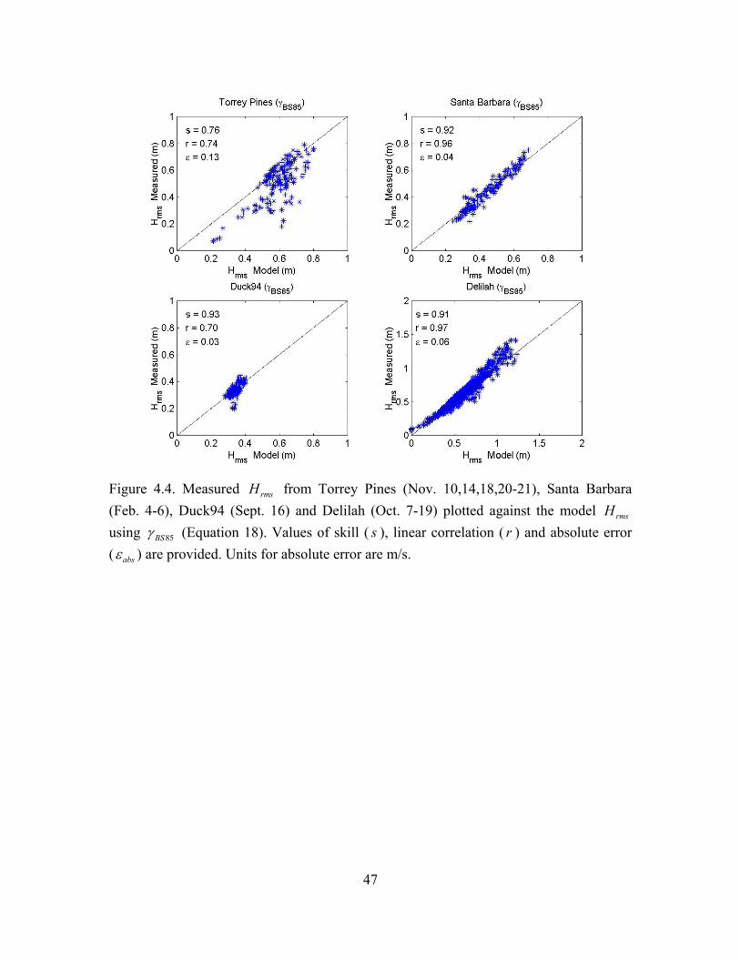
Figure 4.4. Measured from Torrey Pines (Nov. 10,14,18,20-21), Santa Barbara (Feb. 4-6), Duck94 (Sept. 16) and Delilah (Oct. 7-19) plotted against the model using

rmsH

rmsH

85BSγ (Equation 18). Values of skill ( ), linear correlation ( r ) and absolute error (

s

absε ) are provided. Units for absolute error are m/s.

47

Torrey Pines (y_

Hrms Mode'(m)

Santa Barbara (yRcR j BS85'

•0.8

0.6

s ^"o

s = 0.92 r = 0.96 /S

s = 0.04

^^jSMw/l'

«f^ **

0.2 0.4 0.6 0.8 Hrms Mode'(m) Delilah (y

E 1.5

J0.5-

1 1.5 Model (m)

Figure 4.5. Plot of optimized γ versus the Iribarren number (ξ ). Solid line represents parameterization given by Equation 20. Dashed line represents the parameterization given by BS85 (Equation 18) for 0 0.002s < . Dotted lines delineate regions of spilling, plunging and collapsing type waves.

48

Figure 4.6. Measured from Torrey Pines (Nov. 10,14,18,20 and 21), Santa Barbara (Feb. 4,5 and 6) and Duck94 (Sept. 16) plotted against the model using Equation 20. Delilah comparison not included (all ). Values of skill ( ), linear correlation ( r ) and absolute error (

rmsH

rmsH

0 0.002s > sε ) are provided. Units for absolute error are m/s.

49

Figure 4.7. Left panels: fc values based on best fit sk (0.003 m), bed roughness length (0.04 m) and sediment grain size based sk (0.00045 m) during high and low tide on Oct. 10 at Delilah. Middle panels: cross-shore variation of v for 3 sk values. Right panels: alongshore variation of v for 3 sk values.

50

High Tide (OCT 10) High Tide (OCT 10) High Tide (OCT 10) 1.5

150 200 250 300 150 200 250 300 1000 900 800

Low Tide (OCT 10) Low Tide (OCT 10) f

Low Tide (OCT 10)

150 200 250 300 Cross-shore Distance (m)

150 200 250 300 Cross-shore Distance (m)

1000 900 800 Alongshore Distance (m)

Figure 4.8. Left panels: fc values based on best fit sk (0.003 m), bed roughness length (0.04 m) and sediment grain size based sk (0.00045 m) during high and low tide on Oct. 15 at Delilah. Middle panels: cross-shore variation of v for 3 sk values. Right panels: alongshore variation of v for 3 sk values.

51

High Tide (OCT 15) 1

High Tide (OCT 15)

0.5 fay—"sJän- f\r ^s*<E-<^.]>

o l\ ^"^^»-.^.SU

High Tide (OCT 15)

150 200 250 300 150 200 250 300 1000 900 800

Low Tide (OCT 15) Low Tide (OCT 15) Low Tide (OCT 15)

0.5

j^r -^*'>

*

150 200 250 300 Cross-shore Distance (m)

150 200 250 300 Cross-shore Distance (m)

1000 900 800 Alongshore Distance (m)

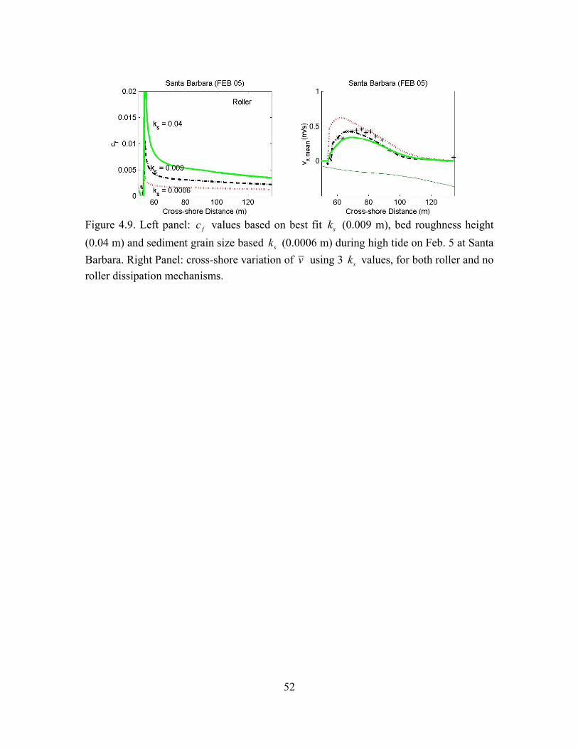
Figure 4.9. Left panel: fc values based on best fit sk (0.009 m), bed roughness height (0.04 m) and sediment grain size based sk (0.0006 m) during high tide on Feb. 5 at Santa Barbara. Right Panel: cross-shore variation of v using 3 sk values, for both roller and no roller dissipation mechanisms.

52

Santa Barbara (FEB 05) 1

Roller

0.015 - ks = 0.04

J" 0.01 - V 0.005 - £*» -—

nL £'=TOö6 • : 60 80 100 120

Cross-shore Distance (m)

Santa Barbara (FEB 05)

60 80 100 120 Cross-shore Distance (m)

Figure 4.10 (a.-f.). Time-lapse video exposures taken during the Delilah experiment (Oct. 7-12). Lightly colored areas represent wave breaking regions owing to shallow depth. The date of the picture is labeled in the right hand corner of each picture, lateral boundaries of the mini-grid are delineated with white lines.

53

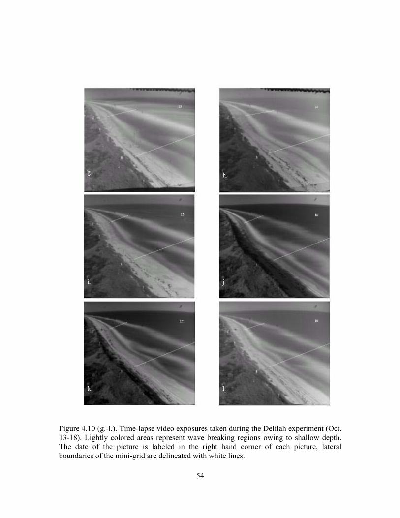
Figure 4.10 (g.-l.). Time-lapse video exposures taken during the Delilah experiment (Oct. 13-18). Lightly colored areas represent wave breaking regions owing to shallow depth. The date of the picture is labeled in the right hand corner of each picture, lateral boundaries of the mini-grid are delineated with white lines.

54

Figure 4.10 (m.). Time-lapse video exposures taken during the Delilah experiment (Oct.19). Lightly colored areas represent wave breaking regions owing to shallow depth. The date of the picture is labeled in the right hand corner of each picture, lateral boundaries of the mini-grid are delineated with white lines.

55

Figure 4.11. Delilah mini-grid bathymetry for Oct.15. Selected current meters labeled for reference. Dotted lines 1-3 denotes cross-shore transects examined for the cross-shore and alongshore momentum balance.

56

Figure 4.12. Model prediction of (solid line) compared with observations (*) for the low (1100) and high (0400) tide of Oct.15 for both no roller and roller dissipation mechanisms. Number in right corner represents model skill.

rmsH

57

No Roller 0.91

1

—>* X

0

Low Tide

*Data

- Model

100 150 200 250 300 Cross-shore Distance (m)

No Roller 0.94

1

f*—*—W £

X 0

High Tide

* Data

- Model

100 150 200 250 300 Cross-shore Distance (m)

100 150 200 250 300 Cross-shore Distance (m)

100 150 200 250 300 Cross-shore Distance (m)

Figure 4.13. Model computed alongshore pressure gradients for the low tide at Delilah on Oct.15. The lighter shades represent positive pressure gradients that act from right to left. Dark shades are negative pressure gradients that act left to right. Circles represent locations of sensors. Symbols R, NR, and MB stand for roller, no roller and measured bathymetry.

58

Figure 4.14. Model computed alongshore pressure gradients for the high tide at Delilah on Oct.15. The lighter shades represent positive pressure gradients that act from right to left. Dark shades are negative pressure gradients that act left to right. Circles represent locations of sensors. Symbols R, NR, and MB stand for roller, no roller and measured bathymetry.

59

Figure 4.15. Measured and model computed cross-shore variation of the alongshore current for low tide (1100) at Delilah on Oct.15. The solid line represents roller dissipation (R) with measured bathymetry (MB), dashed line R with uniform bathymetry (UB), dash-dot line no roller (NR) with MB and dotted line NR with UB. Numbers in right corner represent model skill values. Measured alongshore velocity are indicted by (*). Bathymetry along instrument transect provided as a reference

60

1.5 Case1:RvsNR(UB)

>

1 -

0-

— 0.44 0.31

h\, >* X, i '"HUM»'1' ^F '*?1*^

100 150 200 250 300

1.5

>

1 -

£ 0

Case 3: R vs NR (MB) ■ ■

0.71 —■ 0.6

/3T~T —-^ \ ly^%"""*''-'-•-*,"'*, i"'^.

*^>»*» *

100 150 200 250 Cross-shore Distance (m)

300

Figure 4.16. Measured and model computed cross-shore variation of the alongshore current for the high tide (0400) at Delilah on Oct.15. The solid line represents roller dissipation (R) with measured bathymetry (MB), dashed line R with uniform bathymetry (UB), dash-dot line no roller (NR) with MB and dotted line NR with UB. Numbers in right corner represent model skill values. Instrument bathymetry transect provided as a reference

61

1.5 Casel: RvsNR(UB)

>

1

— 0.71 0.51

Jt *

? '; TW**0** """Pt.frfc,«-

100 150 200 250 300

1.5

>

1

g 0

Case 3: R vs NR (MB) 1 ' 1 '

0.81 _,_, o.74

^ss*.

100 150 200 250 Cross-shore Distance (m)

300

Figure 4.17. Measured cross-shore variation of the alongshore velocity, xv from Delilah (Oct. 7-19) plotted versus model xv . Letter combinations in the title correspond to the following: Roller dissipation (R), No Roller (NR), Measured Bathymetry (MB), Uniform Bathymetry (UB). Numbers in left corner represent the model skill ( ), linear correlation ( r ) and absolute error (

sε ).

62

-0

Delilah R (MB)

s = 0.68 r = 0.89 g /- £ = 0.20 j*

* jH PP ■\dm

Jt^ä&F""** igr 0 1 v Model (m/s)

Delilah R (UB)

vx Model (m/s)

-0

Delilah NR (MB)

s r = £

= 0.43 = 0.76 = 0.35

$vß$

it* /

W*

vx Model (m/s)

Delilah NR (UB)

vx Model (m/s)

Figure 4.18. Oct. 8 model output during low tide for both R(MB) (left panels) and R(UB) (right panels). The dots in the upper panels represent locations of the cross-shore and alongshore instruments. Bottom panels are the corresponding cross-shore transects with measured data (*) plotted versus model output (solid line). Model skill (s) and cross-shore profile provided as a reference.

63

Delilah R(MB)

1200 1000 800 Alongshore Distance (m)

Delilah R(UB)

300

2b0 f^«^«^*******^«-, *#«-, t^***********,*,** ^ *

200 •.*.•.•.•.•.•.•. if •.•.•.•.•.•.•.•.*.*. *-

::::::::•::::::::::i 150 ~~*--«-«-«--«»%«»«-♦-♦-«--«-*- v

n V

100

u ♦ C

1200 1000 800 Alongshore Distance (m)

-2

l -4

-6

100 150 200 250 300 Cross-shore Distance (m)

100 150 200 250 300 Cross-shore Distance (m)

Figure 4.19. Measured and model computed alongshore variation of the alongshore current for the low tide (1100) at Delilah on Oct.15. The solid line represents roller dissipation (R) with measured bathymetry (MB), dashed line R with uniform bathymetry (UB), dash-dot line no roller (NR) with MB and dotted line NR with UB. Numbers in right corner represent model skill values.

64

Figure 4.20. Measured and model computed alongshore variation of the alongshore current for the high tide (0400) at Delilah on Oct.15. The solid line represents roller dissipation (R) with measured bathymetry (MB), dashed line R with uniform bathymetry (UB), dash-dot line no roller (NR) with MB and dotted line NR with UB. Numbers in right corner represent model skill values.

65

Figure 4.21. Measured alongshore variation of the alongshore velocity, yv from Delilah (Oct. 7-19) plotted versus model yv

s

. Letter combinations in the title correspond to the following: Roller dissipation (R), No Roller (NR), Measured Bathymetry (MB), Uniform Bathymetry (UB). Numbers in left corner represent model skill ( ), linear correlation ( r ) and absolute error (ε ).

66

-0

Delilah R (MB)

s = 0.69 ** x r = 0.89 ^^Ä./ - s = 0.22

;; infill BF

%mm* * *

"

v Model (m/s)

Delilah R (UB)

v Model (m/s)

-0

Delilah NR (MB)

s r = £

= 0.40 *^_* / = 0.76 f|ilr+ / - = 0.44 liRjf /

ä*xF±

mm

v Model (m/s)

Delilah NR (UB)

v Model (m/s)

Figure 4.22. Santa Barbara bathymetry for Feb. 4 . Selected current meters labeled for reference. Dotted lines denote cross-shore transects for the cross-shore and alongshore momentum balances.

67

Figure 4.23. Left panel: Model prediction of (solid line) using measured bathymetry compared with observations (*) for the high tide of Feb 4. Right panel: The cross-shore variation of the alongshore current. The number in the lower left hand corner indicates the model skill level. The beach profile is shown as a reference.

rmsH

68

Santa Barbara R(MB)

60 80 100 120

Santa Barbara R(UB)

60 80 100 120

Santa Barbara NR(MB)

100 120

Santa Barbara NR(UB)

100 120

Figure 4.24. Measured and model computed cross-shore variation of the alongshore current for the high tide (1100) at Santa Barbara on Feb 4. The solid line represents roller dissipation (R) with measured bathymetry (MB), dashed line R with uniform bathymetry (UB), dash-dot line no roller (NR) with MB and dotted line NR with UB. Numbers in right corner represent model skill values. Instrument bathymetry transect provided as a reference.

69

1 Casel: RvsNR(UB)

— 0.83 0.84

'S"

ID £

f ***** r **"* 4

60 80 100 120

1r Case 3: RvsNR(MB)

0.84

iv «Äe*, —■ 0.83

F *^**(«

60 80 100 120 Cross-shore Distance (m)

Case 2: NR vs NR (MB/UB)

100 120

Case 4: R vs R (MB/UB)

60 80 100 120 Cross-shore Distance (m)

Figure 4.25. Measured cross-shore variation of the alongshore velocity, xv from Santa Barbara (Feb. 4-6) plotted versus model xv . Letter combinations in the title correspond to the following: Roller dissipation (R), No Roller (NR), Measured Bathymetry (MB), Uniform Bathymetry (UB). Numbers in left corner represent the model skill ( ), linear correlation ( r ) and absolute error (

sε ).

70

0.8

0.6

Santa Barbara R(MB)

£0.4

0.2

s = 0.78

r = 0.88

£ = 0.08

*

#s%% **

0.2 0.4 v. Model

0.6 0.8

Santa Barbara R(UB)

0.4 v. Model

Santa Barbara NR(MB)

0.4 v Model

Santa Barbara NR(UB)

0.2 0.4 0.6 v. Model

Figure 4.26. Top panel: Delilah mini-grid bathymetry for Oct. 15 at low tide overlaid with contours. Middle panel: model computed pressure gradients at low tide. The lighter shades represent positive pressure gradients that act in the direction of wave forcing (right to left). Dark shades are negative pressure gradients that act left to right. Bottom panel: Mean (1 hour) velocities at low tide. The shaded background represents velocity magnitude in m/s.

rmsH

71

Figure 4.27. Top panels: model predicted cross-shore variation of the x-momentum terms Equation 4 for both uniform and measured bathymetry for the low tide (1100) of Oct. 15 transect 1 at Delilah. Bottom panels: cross-shore variation of the y-momentum terms Equation 4 for both uniform and measured bathymetry. Model depth profile provided for reference.

72

Uniform Bathymetry (Low Tide)

150 200 250 300

Uniform Bathymetry (Low Tide)

150 200 250 300

Measured Bathymetry (Low Tide)

150 200 250 300

Measured Bathymetry (Low Tide)

150 200 250 300

Figure 4.28. Top panel: model computed mean alongshore pressure gradients overlaid with the mean velocity computed for Delilah on Oct.15 at low tide. Middle panel: the cross-shore variation of the cross-shore momentum. Bottom panel: the cross-shore variation of the alongshore momentum. Transect lines numbered 1-3 are provided for reference.

73

Cross-shore Momentum (Low Tide)

150 200 250 300 150 200 250 300 150 200 250 300

Alongshore Momentum (Low Tide)

150 200 250 300 150 200 250 300 150 200 250 300

Figure 4.29. Left panel: model predicted cross-shore variation of the x-momentum terms Equation 4 for measured bathymetry for the high tide (1100) of Feb. 4 transect 1 at Santa Barbara. Right panel: cross-shore variation of the y-momentum terms Equation 4 for measured bathymetry. Model depth profile provided for reference.

74

35 Measured Bathymetry (High Tide)

x-momentum

Transect 1

£ 0

Measured Bathymetry (High Tide)

Figure 4.30. Top panel: Santa Barbara bathymetry for Feb. 4 at high tide overlaid with contours. Middle panel: model computed pressure gradients at high tide. The lighter shades represent positive pressure gradients that act opposite the direction of wave forcing (left to right). Dark shades are negative pressure gradients that act right to left. Bottom panel: Mean (1 hour) velocities at high tide. The shaded background represents velocity magnitude in m/s.

rmsH

75

Figure 4.31. Top panel: model computed mean alongshore pressure gradients overlaid with the mean velocity computed for Santa Barbara on Feb. 4 at high tide. Middle panel: the cross-shore variation of the cross-shore momentum. Bottom panel: the cross-shore variation of the alongshore momentum. Transect lines numbered 1-3 are provided for reference.

76

35 x-momentum Transect 1

Measured Bathymetry (High Tide) 35 x-momentum

Transect 2 35 x-momentum

Transect 3

60 80 100 120 60 80 100 120 60 80 100 120

y-momentum Transect 1

y-momentum Transect 2

y-momentum Transect 3

60 80 100 120 60 80 100 120 60 80 100 120

Day ( )rmsH m ( )pf Hz 0s tan β Torrey Pines Nov. 10,14,18,20,21 0.47-0.69 0.06-0.08 0.0011-0.002 0.019-0.025 Santa Barbara Feb. 4-6 0.29-0.65 0.07-0.09 0.001-0.002 0.038-0.043 Delilah Oct. 7-19 0.33-1.76 0.08-0.18 0.003-0.02 0.035 (off) Duck94 Sept. 16 0.28-0.33 0.07 0.0009-0.001 0.066-0.105 (fore) Table 4.1. Wave and beach conditions.

77

Transect xF x

bτ gxη∂∂

uux∂∂

tm uv

y∂∂

Residual

High Tide 1 -472.5 1.3 477.9 0.3 3.0 -2.7 7.2 2 -472.3 1.2 474.4 0.2 2.9 -0.3 6.1 3 -476.0 1.3 478.7 0.5 3.5 -1.6 6.5 Mid Tide 1 -461.0 2.2 478.2 1.1 0.3 -8.3 12.5 2 -461.9 1.7 478.0 0.8 0.7 -4.0 15.3 3 -458.1 1.7 457.6 2.4 -0.4 12.0 15.1 Low Tide 1 -513.4 2.9 528.0 -0.1 0.2 -2.3 15.3 2 -512.1 2.6 526.0 -0.1 -0.1 0.0 16.3 3 -509.9 2.5 524.3 -0.1 -0.1 -0.5 16.3

Table 4.2. Cross-shore integrated cross-shore momentum values using uniform bathymetry for high, mid and low tides at each of the alongshore transects for Delilah on Oct. 15. Units are in N/m.

78

Transect xF x

bτ gxη∂∂

uux∂∂

tm uvy∂∂

Residual

High Tide 1 -479.7 -7.0 574.6 15.8 -4.6 -83.0 16.1 2 -621.9 -10.2 354.9 2.4 0.6 288.1 13.9 3 -578.3 -2.2 397.2 3.4 13.1 180.3 13.7 Mid Tide 1 -517.5 -4.7 592.6 4.3 -4.1 -53.5 17.1 2 -688.6 -12.5 407.5 4.8 -1.1 309.5 19.6 3 -601.8 -0.9 445.0 2.2 11.4 159.7 15.5 Low Tide 1 -551.6 -2.4 617.1 3.4 -4.0 -44.0 18.5 2 -708.2 -11.2 443.4 2.0 1.4 293.2 20.6 3 -612.9 1.5 447.9 0.2 9.4 165.2 11.3

Table 4.3. Cross-shore integrated cross-shore momentum values using measured bathymetry for high, mid and low tides at each of the alongshore transects for Delilah on Oct. 15. Units are in N/m.

79

Transect yF y

bτ gyη∂∂

vvy∂∂

tm vux∂∂

Residual

High Tide 1 89.2 -67.3 -1.5 -10.2 -5.7 -10.4 -5.8 2 89.8 -69.3 0.3 -10.2 -7.0 -9.7 -6.2 3 89.9 -70.7 -2.9 -8.1 -5.1 -9.3 -6.4 Mid Tide 1 105.9 -93.2 -2.0 -12.9 14.8 -7.8 4.8 2 106.4 -96.5 2.4 -16.1 13.4 -4.0 5.5 3 105.6 -98.8 3.2 -10.4 8.5 -1.8 6.4 Low Tide 1 82.0 -75.9 0.6 -10.1 7.6 -8.2 -4.0 2 82.0 -78.5 1.3 -9.2 6.6 -6.3 -4.0 3 81.8 -80.6 1.8 -7.3 5.6 -5.3 -4.0

Table 4.4. Cross-shore integrated alongshore momentum values using uniform bathymetry for high, mid and low tides at each of the alongshore transects for Delilah on Oct. 15. Units are in N/m.

80

Transect yF y

bτ gyη∂∂

vvy∂∂

tm vux∂∂

Residual

High Tide 1 75.7 -81.8 50.1 -55.9 1.2 9.3 -1.4 2 81.7 -79.3 123.7 -124.2 -61.9 61.9 -5.3 3 78.8 -73.6 -32.5 20.6 -6.6 11.3 -1.9 Mid Tide 1 101.4 -100.8 56.8 -61.8 2.5 6.9 5.0 2 117.1 -99.7 166.9 -182.3 -59.3 60.1 2.8 3 98.2 -92.0 -101.8 85.4 3.9 11.8 5.6 Low Tide 1 79.5 -89.8 54.2 -42.6 -1.4 -3.1 -3.2 2 91.4 -85.8 107.2 -110.9 -52.7 46.3 -4.5 3 68.0 -74.4 -78.3 78.0 1.4 2.3 -3.1

Table 4.5. Cross-shore integrated alongshore momentum values using measured bathymetry for high, mid and low tides at each of the alongshore transects for Delilah on Oct. 15. Units are in N/m.

81

Transect xF x

bτ gxη∂∂

uux∂∂

tm uvy∂∂

Residual

High Tide 1 -1578.4 -6.3 1664.7 11.2 -15.4 13.2 89.1 2 -1690.3 13.8 1814.6 0.7 3.7 -49.4 93.1 3 -1657.3 17.5 1750.9 0.0 2.3 -18.6 94.8

Table 4.6. Cross-shore integrated cross-shore momentum values over measured bathymetry at high tide for each of the alongshore transects at Santa Barbara on Feb. 4. Units are in N/m.

82

Transect

yF ybτ g

yη∂∂

vvy∂∂

tm vux∂∂

Residual

High Tide 1 -142.9 118.4 20.8 30.0 19.1 -34.8 10.5 2 -151.4 141.3 35.2 -0.7 -7.0 -9.4 8.0 3 -152.4 140.4 -61.1 48.5 8.3 25.2 8.9

Table 4.7. Cross-shore integrated alongshore momentum values over measured bathymetry at high tide for each of the alongshore transects at Santa Barbara on Feb. 4. Units are in N/m.

83

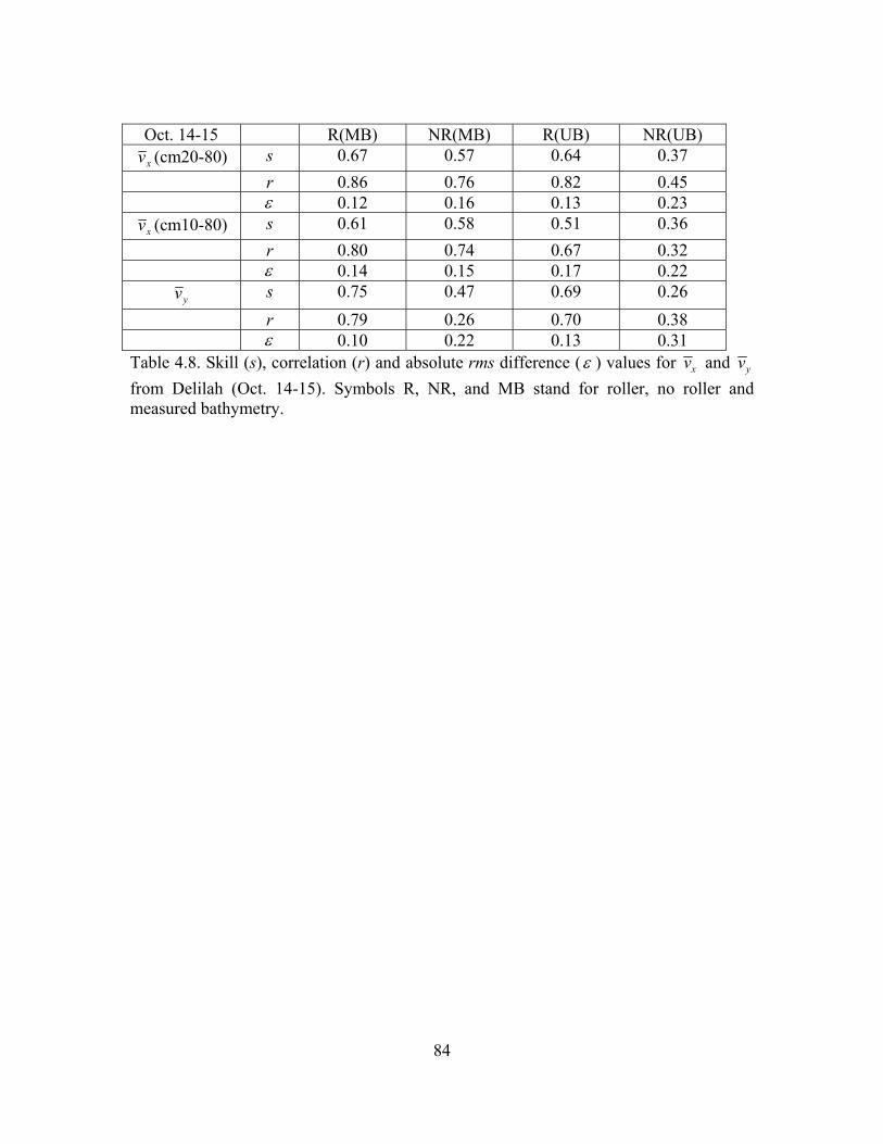
Oct. 14-15 R(MB) NR(MB) R(UB) NR(UB) xv (cm20-80) s 0.67 0.57 0.64 0.37

r 0.86 0.76 0.82 0.45 ε 0.12 0.16 0.13 0.23

xv (cm10-80) s 0.61 0.58 0.51 0.36 r 0.80 0.74 0.67 0.32 ε 0.14 0.15 0.17 0.22 yv s 0.75 0.47 0.69 0.26 r 0.79 0.26 0.70 0.38 ε 0.10 0.22 0.13 0.31

Table 4.8. Skill (s), correlation (r) and absolute rms difference (ε ) values for xv and yv from Delilah (Oct. 14-15). Symbols R, NR, and MB stand for roller, no roller and measured bathymetry.

84

LIST OF REFERENCES

Battjes, J.A., Surf Similarity, in Proc. 14th Int Conf. Coastal Eng., ASCE, pp466-480, New York, 1974.

Battjes, J.A., Modelling of Turbulence in the Surfzone, Proc. Symp. Model. Techniques, San Francisco, 1050-1061, 1975.

Battjes, J.A. and J.P.F.M. Janssen, Energy Loss and Set-up Due to Breaking Waves, in Proceedings of the 16th International Conference Coastal Engineering, p.569, American Society of Civil Engineers, New York, 1978.

Battjes, J.A. and M.J.F. Stive, Calibration and Verification of a Dissipation Model for Random Breaking Waves, J. Geophys. Res., 90, 9159-9167, 1985.

Bowen, A.J., The Generation of Longshore Currents on a Plane Beach, J. Mar. Res., 27, 206-215, 1969.

Church, J.C., and E.B. Thornton, Effects of Breaking Induced Turbulence Within a Longshore Current Model, Coastal Eng., 20, 1-28, 1993.

Deigaard, R., A Note on Three Dimensional Shear Stress Distribution in a Surf Zone, Coastal Eng., 20, 157-171, 1993.

Dingemans, M.W., A.C. Radder and H.J. de Vriend, Computations of the Driving Forces of Wave-induced Currents, Coastal Eng., 11, 539-563, 1987.

Duncan, J.H., An Experimental Investigation of Breaking Waves Produced by a Towed Hydrofoil, Proc. Roy. Lond., A377, 331-348, 1981.

Durand, N. and N.W.H. Allsop, Effects of Steep Bed Slopes on Depth-limited Wave Breaking, Proc. of Waves 97 Conf., Virginia Beach, 1997.

Elgar, S.E., R.T. Guza, B. Raubenheimer, T.H.C. Herbers and E.L. Gallagher, Spectral Evolution of Shoaling and Breaking Waves on a Barred Beach, J. Geophys. Res., 102, 15797-15805, 1997

Feddersen, F., R.T. Guza, S. Elgar and T.H.C. Herbers, Alongshore Momentum Balances in the Nearshore, J. Geophys. Res., 103, 15667-15676, 1998.

Fredsoe, J., Turbulent Boundary Layer in Wave-Current Motion, J. Hydraul. Eng. ASCE, 110, 1103-1120, 1984.

Gallagher, E.L., E.B. Thornton and T.P. Stanton, Sand Bed Roughness in the Nearshore, submitted to J. Geophys. Res.

Garcez-Faria, A.F., E.B. Thornton, T.P. Stanton, C.V. Soares and T.C. Lippmann, Vertical Profiles of Longshore Currents and Related Bed Shear Stress and Bottom Roughness, J. Geophys. Res., 103, 3217-3232, 1998.

Guza, R.T. and E.B. Thornton, Local and Shoaled Conaprisons of Sea Surface Elevations, Pressures and Velocities, J. Geophs. Res., 85, 1524-1530, 1980.

85

Holthuijsen, L.H., N. Booij and T.H.C. Herbers, A Prediction Model for Stationary, Short-Crested Waves in Shallow Water with Ambient Currents, Coastal Eng., 13, 23-54. 1989.

Lippmann, T.C., A.H. Brookins and E.B. Thornton, Wave Energy Transformation on Natural Profiles, Coastal Eng., 27, 1-20, 1996.

Long, C.E., Index and Bulk Parameters for Frequency-direction spectra Measured at CERC Field Research Facility, September 1990 to August 1991, Misc Pap., CERC-94-5, U.S. Army Eng. Waterw. Exp. Stn., Vicksburg, Miss., 1994.

Longuet-Higgins, M.S., Longshore Currents Generated by Obliquely Incident Sea Waves, 1, J. Geophys. Res., 75, 6778-6789, 1970.

Nairn, R.B., J.A. Roelvink and H.N. Southgate, Transition Zone Width and Implications for Modeling Surfzone Hydrodynamics, Proc. 22nd Int. Conf. Coastal Eng., New York, 68-81, 1990.

Nicholson, J., I. Broker, J.A. Roelvink, D. Price, J.M. Tanguy and L. Moreno, Intercomparison of Coastal Area Morphodynamic Models, Coastal Eng., 31, 97-123, 1997.

Putrevu, U., J. Oltmay-Shay and I.A. Svendsen, Effects of Alongshore Nonuniformities on Longshore Current Predictions, J. Geophys. Res., 100, C8, 16119-16130, 1995.

Reniers, A.J.H.M. and J.A. Battjes, A Laboratory Study of Longshore Currents Over Barred and Non-Barred Beaches, J. of Coastal Eng., vol 30, 1-22, 1997.

Reniers, A.J.H.M., Longshore Current Dynamics, Ph.D. Dissertation, Communications on Hydraulic and Geotechnical Engineering, Fac of Civil Engineering and Geosciences, Report no. 99-2, ISSN 0169-6548, 133p.

Sancho, F.E., I.A. Svendsen, A.R. Van Dongeren and U. Putrevu, Longshore Non-uniformities of Nearshore Currents, in Coastal Dynamics 1995, pp425-436, Am. Soc. Of Civ. Eng., New York, 1995.

Slinn, D.N., J.S. Allen and R.A. Holman, Alongshore Currents Over Variable Beach Topography, J. Geophys.Res., 105, 16971-16998, 2000.

Smith, J.M., M. Larson and N.C. Kraus, Longshore Current on a Barred Beach: Field Measurements and Calculations, J. Geophys. Res., 98, 22,717-22,731, 1993.

Soulsby, R.L., L. Hamm, G. Klopman, D. Myrhaug, R.R. Simons and G.P. Thomas, Wave-Current Interaction Within and Outside the Bottom Boundary Layer, Coastal Eng., 21, 41-69, 1993.

Soulsby, R.L., Dynamics of Marine Sands, Telford, 1997.

Stelling, G.S., On the Construction of Computational Methods for Shallow Water Flow Problems, Rijkswaterstaat Communications, No 35, 1984.

Svendsen, I.A., Wave Heights and Set-up in a Surfzone, Coastal Eng., 8, 303-329, 1984.

Thornton, E.B., Variation of Longshore Current Across the Surf Zone, in Proc. 12th Int Coastal Engineering Conf., pp. 291-308, Am. Soc. of Civ. Eng., New York, 1970.

86

Thornton, E.B. and R.T. Guza, Transformation of Wave Height Distribution, J. Geophys. Res., 88, 5925-5938, 1983.

Thornton, E.B. and R.T. Guza, Surf-zone Longshore Currents and Random Waves: Field Data and Models, J. Phys. Oceanogr., 16, 1165-1178, 1986.

Verboom, G.K. and A. Slob, Weakly-reflective Boundary Conditions for Two-dimensional Water Flow Problems, 5th Int. Conf. On Finite Elements in Water Resources, 1984.

Whitford, D.J., and E.B. Thornton, Comparison of Wind and Wave Forcing of Longshore Currents, Cont. Shelf. Res., 13, 1205-1218, 1993.

Whitford, D.J., and E.B. Thornton, Bed Shear Stress Coefficients for Longshore Currents Over a Barred Beach, Coastal Eng., 27, 243-262, 1996.

87

THIS PAGE INTENTIONALLY LEFT BLANK

88

INITIAL DISTRIBUTION LIST

1. Defense Technical Information Center....................................................................2 8725 John J. Kingman Road, Suite 0944 Ft. Belvoir, VA 22060-6218

2. Dudley Knox Library...............................................................................................2 Naval Postgraduate School 411 Dyer Road Monterey, CA 93943-5101

3. Distinguished Professor Edward B. Thornton Department of Oceanography, Naval Postgraduate School thornton@nps.navy.mil

4. Doctor Adrianus Reniers

Department of Oceanography, Naval Postgraduate School reniers@nps.navy.mil

89