Embed Size (px)
Citation preview

Ing. Milan Hanus
Mathematical Modeling ofNeutron Transport
Field of study
Applied Mathematics
Submitted in partial fulfillment
of the requirements for the degree of
Doctor of Philosophy (Applied Mathematics)
Pilsen, January 6th, 2015

The dissertation thesis was prepared as a part of a doctoral program Applied Mathemat-ics at the Department of Mathematics, Faculty of Applied Sciences, University of WestBohemia in Pilsen, Czech Republic.
Applicant: Ing. Milan HanusDepartment of MathematicsFaculty of Applied SciencesUniversity of West Bohemia in PilsenUniverzitni 22, 306 14 Pilsen, Czech Rep.
Supervisor: doc. Ing. Marek Brandner, Ph.D.Department of MathematicsFaculty of Applied SciencesUniversity of West Bohemia in PilsenUniverzitni 22, 306 14 Pilsen, Czech Rep.
Reviewers: doc. RNDr. Ivana Pultarova, Ph.D.Department of MathematicsFaculty of Civil EngineeringCzech Technical University in PragueThakurova 7, 166 29 Prague 6, Czech Rep.
Ryan G. McClarren, Ph.D.Department of Nuclear EngineeringTexas A&M University253 Bizzell West, 3133 TAMUCollege Station, US-TX 77843-3133
The report was distributed on: . . . . . . . . . . . . . . . . . . . . . . . . .
The defense of the dissertation thesis is scheduled for . . . . . . . . . . . . . . . . . . . . . . . . in front ofthe committee of Applied Mathematics at the Faculty of Applied Sciences, University ofWest Bohemia in Pilsen, Univerzitni 22, 306 14 Pilsen, Czech Rep., in room
. . . . . . . . . . . . . . . . . . . . . . . . at . . . . . . . . . . . . . . . . . . . . . . . . .
The dissertation thesis will be available at the Department of Ph.D. Study of the Universityof West Bohemia, Univerzitni 22, UV 206.
prof. RNDr. Pavel Drabek, DrSc.Head of the branch board for Applied Mathematics
v

Declaration
I hereby declare that this doctoral thesis is my own work, unless clearly statedotherwise.
. . . . . . . . . . . . . . . . . . . . . . . . . . .Ing. Milan Hanus
vi
Abstract
The subject of this work is computational modeling of neutron transport rele-vant to economical and safe operation of nuclear facilities. The general math-ematical model of neutron transport is provided by the linear Boltzmann’stransport equation and the thesis begins with its precise mathematical formu-lation and presentation of known conditions for its well-posedness.
In the following part, we study approximation methods for the transport equa-tion, starting with the classical discretization of energetic dependence and fol-lowed by the review of two most widely used methods for approximating direc-tional dependence (the SN and PN methods). While these methods are usuallypresented independently of each other, we show that they can be put into asingle framework of Hilbert space projection techniques. This fact is then usedin conjunction with the results of the first part to rigorously prove rotationalinvariance of the PN equations and to analyze convergence of the basic iterativescheme for solving the SN equations. This part is concluded by the descriptionof a finite element method for the final discretization of spatial dependence anda discussion of solution of the resulting system of algebraic equations.
The main new results are contained in the following two chapters focusing on thesimplified PN approximation, which is a computationally more convenient albeitnot as mathematically well-founded variant of the PN approximation. We provewell-posedness of the weak form of the SP3−7 equations and present a new wayof deriving the equations from an alternative set to the PN equations, obtainedfrom special linear combination of spherical harmonics – the so-called Maxwell-Cartesian spherical harmonics, hence the abbreviation MCPN . We explicitlyshow how the MCP3 equations may be transformed to the SP3 equations.
The final part of the thesis contains numerical examples of the SN and hp-adaptive SPN calculations using a neutronics framework that has been imple-mented by the author to the hp-adaptive finite element library Hermes2D. TheSP1 (or diffusion) model also serves as a basis of a real-world reactor calculationsuite co-developed by the author for the purposes of “Project TA01020352 –Increasing utilization of nuclear fuel through optimization of an inner fuel cycleand calculation of neutron-physics characteristics of nuclear reactor cores”. Anexample benchmark used to test the code concludes the thesis.
vii
Keywords:
Neutron transport, Boltzmann equation, reactor criticality, multigroup approx-imation, PN approximation, simplified PN approximation, discrete ordinates,ray effects, source iteration, angular quadrature, projection, diffusion, sphericalharmonics, well-posedness, weak formulation, Maxwell-Cartesian spherical har-monics, tensor, MCPN approximation, finite elements, discontinuous Galerkinmethod, hp-adaptivity, algebraic multigrid, Hermes2D, Dolfin.
Main Goals:
The main goal of the thesis is to investigate the feasibility of using finite elementmethod for solving neutron transport problems. Particular emphasis is put onsolving problems appearing in reactor criticality studies. The goals can besummarized in the following items.
• Investigate existing neutron transport approximations and their suitabilityfor reactor-scale calculations.
• Describe mathematical properties of these approximations that have im-portant consequences for actual numerical solution.
• Provide more thorough analysis of the simplified PN approximation (SPN).
• Implement and evaluate finite element solvers based on the SPN approxi-mation.
viii
Abstrakt
Prace se zabyva matematickym a numerickym modelovanım transportu ne-utronu, se zamerenım na vypocty neutronovych charakteristik jadernych reak-toru. Obecny matematicky model transportu neutronu je reprezentovan linearnıBoltzmannovou transportnı rovnicı. Prace zacına jejı presnou matematickouformulaci a prehledem vysledku tykajıcıch se jejı resitelnosti ve druhe kapitole.Nasledujıcı kapitoly jsou zamereny na priblizne metody resenı teto rovnice.
Po strucnem popisu klasicke diskretizace energeticke zavislosti je hlavnı casttretı kapitoly venovana aproximaci smerove zavislosti pomocı dvou metod – me-tody diskretnıch ordinat (SN) a metody sferickych harmonickych funkcı (PN).Zatımco obvykle jsou tyto metody formulovany nezavisle, v praci je ukazano,jak je lze obe popsat pomocı jednotneho ramce jako projekci na podprostorHilbertova prostoru funkcı definovanych na sfere. Teto skutecnosti je vyuzitopri dukazu rotacnı invariantnosti PN rovnic a pri analyze konvergence zakladnıiteracnı metody pro resenı SN soustavy. Tretı kapitola je zakoncena popisemaplikace metody konecnych prvku na finalnı diskretizaci prostorove zavislosti.
Hlavnı nove vysledky teto prace se tykajı metody zjednodusenych sferickychharmonickych funkcı (SPN), jez predstavuje vypocetne efektivnı aproximacimetody PN . Ve ctvrte kapitole je standardnım zpusobem odvozena slaba for-mulace SPN rovnic a dokazana jejı korektnost pro N = 3, 5, 7. V pate kapitole jepak odvozena nova soustava parcialnıch diferencialnıch rovnic odpovıdajıcı PN
aproximaci (MCPN aproximace). Na prıkladu MCP3 aproximace je ukazano,jak lze vyuzıt tenzorovou strukturu techto rovnic k transformaci na soustavuekvivalentnı s SP3 aproximacı.
V seste kapitole je popsana implementace SN a SPN aproximacı do knihovnyHermes2D a na nekolika prıkladech ukazany zakladnı vlastnosti techto apro-ximacı. Specialnı pozornost je venovana implementaci nespojite Galerkinovymetody (pro SN aproximaci)a modifikaci standardnıho indikatoru chyby prohp-adaptivitu v Hermes2D pro SPN aproximaci. Prace je ukoncena ukazkouresenı standardnıho 3D benchmarku pomocı mnohagrupoveho difuznıho kodu,ktery autor na zaklade zkusenostı s vyvojem neutronickych modulu v knihovneHermes2D vyvinul pro ucely projektu “TA01020352 – Zvysenı vyuzitı jadernehopaliva pomocı optimalizace vnitrnıho palivoveho cyklu a vypoctu neutronove-fyzikalnıch charakt. aktivnıch zon jadernych reaktoru”.
ix
Klıcova slova:
Transport neutronu, Boltzmannova rovnice, kriticnost reaktoru, vıcegrupovaaproximace, PN aproximace, zjednodusena PN aproximace, metoda diskretnıchsmeru, iterace zdroje, ray efekt, smerova kvadratura, projekce, difuze, sferickeharmonicke funkce, korektnost, slaba formulace, Maxwellovy kartezske sferickeharmonicke funkce, tenzor, MCPN aproximace, konecne prvky, nespojita Galer-kinova metoda, hp-adaptivita, algebraicka metoda vıce sıtı, Hermes2D, Dolfin.
Hlavnı cıle:
Hlavnım cılem teto prace je posouzenı moznosti pouzitı metody konecnychprvku pro resenı uloh transportu neutronu. Specialnı pozornost je venovanauloham na kriticnost jadernych reaktoru. Cıle prace jsou shrnuty v nasledujıcıchbodech.
• Posouzenı vhodnosti existujıcıch aproximacı transportu neutronu pro re-aktorove vypocty.
• Popis matematickych vlastnostı zvolenych aproximacı, jez jsou podstatnepro vlastnı numericke vypocty.
• Podrobnejsı analyza zjednodusene PN aproximace (SPN).
• Implementace a pouzitı konecne-prvkoveho resice zalozeneho na SPN apro-ximaci.
x
CONTENTS
Contents
1 Introduction 1
2 Mathematical model of neutron transport 42.1 Neutron transport equation . . . . . . . . . . . . . . . . . . . . . . . . . . 42.2 Neutronic phase space . . . . . . . . . . . . . . . . . . . . . . . . . . . . . 42.3 Boundary conditions . . . . . . . . . . . . . . . . . . . . . . . . . . . . . . 62.4 Collision terms . . . . . . . . . . . . . . . . . . . . . . . . . . . . . . . . . 62.5 Quantities of interest . . . . . . . . . . . . . . . . . . . . . . . . . . . . . . 72.6 Neutron transport problems . . . . . . . . . . . . . . . . . . . . . . . . . . 8
2.6.1 Fixed source problem . . . . . . . . . . . . . . . . . . . . . . . . . . 92.6.2 Criticality problem . . . . . . . . . . . . . . . . . . . . . . . . . . . 10
2.7 Rotational invariance of the NTE . . . . . . . . . . . . . . . . . . . . . . . 12
3 Neutron transport approximations 133.1 Approximation of energetic dependence . . . . . . . . . . . . . . . . . . . . 13
3.1.1 Criticality problems . . . . . . . . . . . . . . . . . . . . . . . . . . . 143.1.2 Group source iteration . . . . . . . . . . . . . . . . . . . . . . . . . 15
3.2 The PN method . . . . . . . . . . . . . . . . . . . . . . . . . . . . . . . . . 153.2.1 Operator form . . . . . . . . . . . . . . . . . . . . . . . . . . . . . . 173.2.2 Structure of the PN system . . . . . . . . . . . . . . . . . . . . . . 183.2.3 Diffusion approximation . . . . . . . . . . . . . . . . . . . . . . . . 19
3.3 The SN method . . . . . . . . . . . . . . . . . . . . . . . . . . . . . . . . . 203.3.1 Structure of the SN system . . . . . . . . . . . . . . . . . . . . . . . 213.3.2 Operator form . . . . . . . . . . . . . . . . . . . . . . . . . . . . . . 213.3.3 Convergence of the source iteration . . . . . . . . . . . . . . . . . . 223.3.4 Discontinuous Galerkin method for the SN approximation . . . . . 23
4 The simplified PN approximation 254.1 The SP3 approximation . . . . . . . . . . . . . . . . . . . . . . . . . . . . . 25
5 The MCPN approximation 285.1 Maxwell-Cartesian spherical harmonics . . . . . . . . . . . . . . . . . . . . 285.2 MCPN approximation . . . . . . . . . . . . . . . . . . . . . . . . . . . . . 295.3 The MCP3 system . . . . . . . . . . . . . . . . . . . . . . . . . . . . . . . 31
6 Neutronics modules 336.1 Hermes2D modules . . . . . . . . . . . . . . . . . . . . . . . . . . . . . . . 336.2 SPN and diffusion examples . . . . . . . . . . . . . . . . . . . . . . . . . . 34
6.2.1 Benchmark IAEA EIR-1 . . . . . . . . . . . . . . . . . . . . . . . . 346.2.2 The 7× 7 PWR assembly example (Stankovski benchmark) . . . . 386.2.3 Two-group WWER-440 criticality benchmark (diffusion) . . . . . . 43
6.3 SN example . . . . . . . . . . . . . . . . . . . . . . . . . . . . . . . . . . . 46
xi

CONTENTS
6.3.1 Watanabe-Maynard Problem 1 . . . . . . . . . . . . . . . . . . . . 466.4 Coupled code system for quasi-static whole-core calculations . . . . . . . . 49
7 Summary 51
Index 59
xii
1 Introduction
1 Introduction
Computer simulation of radiative transfer of energy is an important task in many en-
gineering and research areas, as diverse as biomedicine, astrophysics, optics or nuclear
engineering. In nuclear engineering, the topical area of the presented thesis, there are two
main goals of computer modeling of radiative transfer. The first is to simulate short-term
transient behavior of nuclear devices under given initial conditions such as geometry and
material configuration. The second is to determine under which conditions such devices
(in this case typically nuclear reactor cores) will be capable of long-term, stable operation
satisfying certain safety, technical and economical limitations, with only a minimal human
intervention. Repeated calculations of the second type form the basis for designing new
nuclear reactors or optimizing fuel reloading of existing ones. Optimization of fuel reload-
ing schemes for nuclear reactors is the topic of a major research and development project
investigated at author’s department1. Author’s participation in this project involved the
development of a neutron-physical calculation module that could be employed by the over-
all optimization suite to evaluate fitness of its candidate configurations. This fact largely
influenced the choice of mathematical models and numerical methods studied in the thesis.
The most accurate mathematical description of the relevant physical processes is pro-
vided by the linear Boltzmann transport equation. As the primary application domain
of interest is the simulation of long-term behavior of nuclear reactors driven by neutron-
induced reactions, a particular form of the equation – the steady state neutron transport
equation (shortly NTE) – is specifically considered in the thesis. We note, however, that
methods described in the work provide basic building blocks of time-dependent calculations
as well as of simulations involving other mutually non-interacting particles like photons.
Mathematical modelling of neutron transport
The steady state NTE is introduced in the second chapter of the thesis as an integro-
differential equation with 6 independent variables (three characterizing position of neu-
trons, two their streaming direction and one their energy) and its theoretical properties
are reviewed. The high dimensionality of the equation requires either a direct particle sim-
ulation and use of statistical methods for obtaining the required physical quantities (the
Monte Carlo approach) or a deterministic approach involving multiple discretizations. As
1Project TA01020352 – Increasing utilization of nuclear fuel through optimization of an inner fuel
cycle and calculation of neutron-physics characteristics of nuclear reactor cores. Principal investigators:
R. Cada (University of West Bohemia) and J. Rataj (Czech Technical University).
1
1 Introduction
the second approach is still preferable in terms of overall efficiency, it has been chosen as
the subject matter of the thesis.
The work focuses on two widely used methods of this category – the method of spherical
harmonics, abbreviated PN and the method of discrete ordinates, abbreviated SN . Both
can be viewed as projections of the NTE onto a particular Hilbert subspace of L2(S2) –
the space of square integrable functions of the directional variables. This is the way how
the PN method is usually presented, but it is not immediately obvious in the SN case, as
described in the third chapter of the thesis.
The subspace projection interpretation of both methods has been used to study their
numerical behavior by translating properties of the continuous NTE to the discrete case.
As a first application, we give a proof of rotational invariance property of the PN ap-
proximation. This is a well known fact preventing the undesirable “ray effects” of the
rotationally non-invariant SN approximation, of which we however couldn’t find a formal
proof in available literature. As a second application, we analyze convergence of a classical
iterative method for the SN approximation by direct application of a Banach fixed-point
argument proved for the continuous NTE in [22] (i.e. using a different approach than the
usual one based on Fourier analysis in an infinite medium).
The MCPN approximation and its relation to the SPN approximation
A new set of equations equivalent to the original PN set has been derived in Chapter 5.
The derivation starts by choosing an alternative approximation basis, composed of special
linear combinations of the original basis used in the PN approximation. These new basis
functions (the Maxwell-Cartesian surface spherical harmonics introduced in [4]) have a
clear tensorial structure formally resembling that of Legendre polynomials and lead to a
set of equations resembling the 1D PN equations. We call this set the MCPN approximation
(“Maxwell-Cartesian PN” approximation) and use its structure to uncover its connection to
another traditional approximation of neutron transport – the simplified spherical harmonic
method, shortly SPN .
The SPN method (particularly the SP3) already simplifies the NTE to the extent that
it is applicable to day-by-day whole-core calculations on usual workstations with a few
computational cores or small-scale servers with tens of cores. SPN equations are studied
in the fourth chapter, with the focus on their weak formulation needed for the finite-
element spatial discretization (including an original proof of its well-posedness for the
most important cases N = 3, 5, 7, with a straightforward extension to higher orders). As
2
1 Introduction
recalled in that chapter, when the SP3 method is used for typical reactor core calculations,
its solution captures most of the features of the true solution of the NTE. Combined
with its efficiency, this makes it attractive for physicists to quickly test their empirical
approximations used throughout their production code, which is usually based on the
most restricting transport approximation – the diffusion approximation.
Finite element framework for neutron diffusion/transport
The neutron diffusion approximation, whereby the NTE is reduced to a second-order elliptic
PDE (or, when energy dependence is taken into account implicitly, a weakly coupled non-
symmetric system of second-order PDEs with positive-definite symmetric part – the so-
called multigroup neutron diffusion approximation recalled in Chapter 3), also forms the
basis of the neutronics module prepared for the above mentioned nuclear reactor fuel usage
optimization code. The finite element method has been used to obtain the final discrete
algebraic system of equations. This distinguishes it from the majority of other codes used
for similar purposes, which are usually based on the so-called nodal method [31, 39] and
allowed us to circumvent some deficiencies of nodal methods, such as limited geometrical
flexibility, need for reconstruction procedure or stability and convergence issues.
Nevertheless, the basic principle underlying the nodal method – computing two solu-
tions with different accuracy to provide a more accurate one – still guided the initial choice
of finite element library on which to base the neutronics modules. This led the author to
the open-source finite element C++ library Hermes2D [23], which uses that principle to
drive its advanced hp-adaptivity procedure [48]. Combined with its unique way of assem-
bling coupled systems of PDEs [50], the Hermes2D library has proved to be well-suited for
testing the neutronic approximations described in the first part of the thesis.
The final chapter of the thesis describes the neutronics framework, simplifying and
unifying the formulation of multiregion, multigroup neutron diffusion, SPN or SN problems
within Hermes2D. It also discusses additions to the library required by these modules
(like the discontinuous Galerkin assembling for the SN module) as well as hp-adaptivity
tailoring for the SPN equations. As the 3D version of Hermes is still a work in progress,
the three-dimensional whole-core neutron diffusion solver required by the above mentioned
project on nuclear reactor fuel usage optimization has been ultimately developed under
the FEniCS/Dolfin framework ([40, 41]). Some of its features (such as MPI parallelism or
quasi-static solution with thermal/hydraulic feedback) are discussed and demonstrated on
the solution of a standard neutronics benchmark in the concluding part of the thesis.
3
2 Mathematical model of neutron transport
2 Mathematical model of neutron transport
2.1 Neutron transport equation
The steady state neutron transport equation is a mathematical representation of balance
between neutron gains and losses within a given macroscopic domain D ⊂ R3. Let us
consider the equation in its integro-differential form with given neutron source function q:
Ω · ∇ψ(r,Ω, E) + σt(r, E)ψ(r,Ω, E) =
=
∫ Emax
Emin
∫S2κ(r,Ω ·Ω′, E E ′)ψ(r,Ω′, E ′) dΩ′ dE ′ + q(r,Ω, E), r ∈ D.3
(1)
Function σt groups all reactions that result in a loss of neutron and is called total (macro-
scopic) cross-section, while κ represents reactions that introduce neutrons into direction Ω
and energy E by scattering from direction Ω′, slowing down (or accelerating) from higher
(lower) energies E ′ or releasing new neutrons from fissioned nuclei.
Solution of eq. (1), the angular neutron flux density ψ – is a function of the following
independent variables, which define the neutron phase space:
• r = (x, y, z) represents the spatial distribution of neutrons,
• Ω represents the angular distribution of neutrons on a unit sphere S2, i.e. their
streaming direction (Ω ∈ R3, ‖Ω‖ = 1);
• E ∈ [Emin, Emax] is the kinetic energy of neutrons.
Since the direction vectors are confined to the sphere, we can express the three Cartesian
components of Ω by only two spherical coordinates ϑ ∈ [0, π] and ϕ ∈ [0, 2π):
Ω =
Ωx
Ωy
Ωz
=
sinϑ cosϕsinϑ sinϕ
cosϑ
.2.2 Neutronic phase space
Let us assume that D is a domain bounded by a piecewise smooth boundary ∂D, which is
oriented at almost every point r ∈ ∂D (a.e. in ∂D) by its unit outward normal field n(r).
Then we may formally define the neutron phase space
X := (r,Ω, E) : r ∈ D ⊂ R3,Ω ∈ S2, E ∈ [Emin, Emax]3Boundary conditions will be described in Sec. 2.3.
4
2.2 Neutronic phase space
together with its outflow and inflow boundary subsets, respectively:
∂X± :=
(r,Ω, E) ∈ ∂D × S2 × [Emin, Emax], s.t. Ω · n(r) ≷ 0.
The whole boundary ∂X can be written as
∂X = ∂X+ ∪ ∂X− ∪ ∂X0
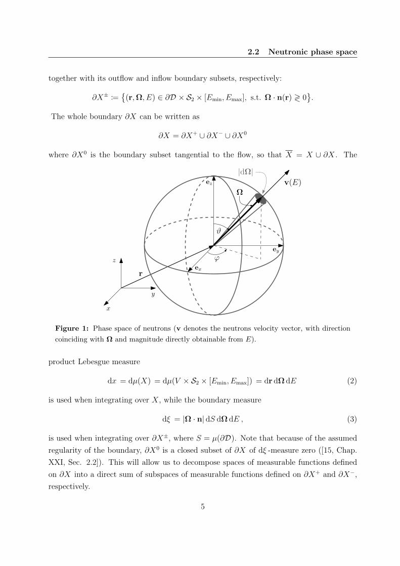
where ∂X0 is the boundary subset tangential to the flow, so that X = X ∪ ∂X . The
x
y
zex
ey
ez
r
v(E)Ω
|dΩ|
ϕ
ϑ
Figure 1: Phase space of neutrons (v denotes the neutrons velocity vector, with direction
coinciding with Ω and magnitude directly obtainable from E).
product Lebesgue measure
dx = dµ(X) = dµ(V × S2 × [Emin, Emax]) = dr dΩ dE (2)
is used when integrating over X, while the boundary measure
dξ = |Ω · n| dS dΩ dE , (3)
is used when integrating over ∂X±, where S = µ(∂D). Note that because of the assumed
regularity of the boundary, ∂X0 is a closed subset of ∂X of dξ -measure zero ([15, Chap.
XXI, Sec. 2.2]). This will allow us to decompose spaces of measurable functions defined
on ∂X into a direct sum of subspaces of measurable functions defined on ∂X+ and ∂X−,
respectively.
5
2 Mathematical model of neutron transport
2.3 Boundary conditions
In order to formulate well-posed neutron transport problems, we consider equation (1)
together with the following types of boundary conditions, specified at the inflow boundary
∂X−:
• incoming angular neutron flux
ψ|∂X− = ψin (4)
(ψin ≡ 0 corresponds to vacuum in R3 \D, which is a common assumption in nuclear
reactor modeling),
• albedo boundary reflection
ψ(r,Ω, E) = β(r)ψ(r,ΩR, E), (r,Ω, E) ∈ ∂X−, ΩR = Ω− 2n(Ω · n) (5)
where Ω is the reflection of ΩR about the boundary plane. For β ≡ 1, this corresponds
to complete specular reflection and is used to model planes of symmetry, while for
β ≡ 0, we recover the vacuum condition from above. Intermediate values mean that a
fraction of neutrons leaving the domain in direction ΩR are returned back in direction
Ω, which is commonly used to model reactor reflectors. We thus assume 0 ≤ β ≤ 1.
For description of other types of boundary conditions, we refer to [54] or [2, Sec. 1.3].
2.4 Collision terms
In writing equation (1), we used the assumption that the medium filling D is isotropic,
hence the collision kernel κ depends on the incoming and outgoing directions only through
their inner product Ω ·Ω′, and the dependence of σt on Ω need not be considered. Further
physical assumptions, valid in applications of interest to us4, yield the following splitting
κ(r,Ω ·Ω′, E E ′) = σs(r,Ω ·Ω′, E E ′) +χ(E)νσf (r, E
′)
4π. (6)
Let us first consider the fission part – σf is the fission cross-section (σf (r, E′) characterizes
the probability that neutrons with energy E ′ induce a fission reaction at r, with arbitrary
resulting energetic distribution), ν is the mean number of neutrons released from fission
and χ(E) represents the probability that fission neutrons will be released with energy E
(fission spectrum,∫ Emax
Eminχ(E) dE = 1).
4elastic scattering dominates inelastic, fission is an isotropic process
6
2.5 Quantities of interest
Unlike fission, scattering is in general not an isotropic process; nevertheless, we still
define the scattering cross-section as
σs(r, E) =
∫ Emax
Emin
∫S2σs(r,Ω
′ ·Ω, E ′ E) dΩ′ dE ′ ,
characterizing the probability of neutrons with energy E ′ inducing scattering at r (irre-
spective to the resulting energetic and angular distribution). Then
σt(r, E) = σc(r, E) + σf (r, E) + σs(r, E) ≡ σa(r, E) + σs(r, E) (7)
where
• σc(r, E) is the non-productive capture cross section (resulting in no new neutrons
being introduced into the system) and
• σa(r, E) = σc(r, E) + σf (r, E) is the absorption cross section.
2.5 Quantities of interest
From angular flux ψ, one can derive the following important integral quantities
• scalar neutron flux (density)
φ(r, E) =
∫S2ψ(r,Ω, E) dΩ , (8)
• net neutron current (density)
J(r, E) =
∫S2
Ωψ(r,Ω, E) dΩ , (9)
• reaction rate (density) (per unit time) of given type (x = t, a, f, s, c, see eq. (7)),
induced by neutrons of energies in range [E1, E2]∫ E2
E1
σx(r, E)φ(r, E) dE . (10)
Scalar flux and reaction rates may be experimentally measured by various detector mecha-
nisms, which is the reason why these quantities are more important in practical calculations
than the angular neutron flux ψ.
7
2 Mathematical model of neutron transport
2.6 Neutron transport problems
In this section, we formulate two fundamental neutron transport problems and recall known
results about their unique solvability. We note that one can generally expect only very
low regularity of the exact solution of the NTE. Therefore, we will consider the generalized
solutions of these problems (which we call just solutions), which satisfy the equation and
boundary conditions almost everywhere (a.e.) in X (or ∂X ).
Let us define the following operators:
Aψ(r,Ω, E) = Ω · ∇ψ(r,Ω, E),
Σtψ(r,Ω, E) = σt(r, E)ψ(r,Ω, E),
Kψ(r,Ω, E) =
∫ Emax
Emin
∫S2κ(r,Ω ·Ω′, E E ′)ψ(r,Ω′, E ′) dΩ′ dE ′ .
We call A, Σt, K and T := A+Σt−K the advection, reaction, collision and transport opera-
tor, respectively. All these operators are linear; the reaction operator Σt : Lp(X)→ Lp(X)
is a bounded self-adjoint multiplication operator in Lp(X) (the standard Lebesgue space
with index p w.r.t. the measure (2)), while the operator K : Lp(X)→ Lp(X) is bounded
under additional (physically justifiable) conditions (conditions (c) and/or (d) of Def. 1,
depending on p). It is self-adjoint if and only if the kernel κ of K is symmetric in E and
E ′. With the exception of the monoenergetic case, this is generally not true. To further
simplify notation, let
L := A+ Σt.
For piecewise smooth ∂D and 1 ≤ p <∞, the results of [15, Thm. 1, Appendix of §2,
Chap. XXI] or [6] ensure existence of spaces
Hp(X) = ψ | ψ ∈ Lp(X),Ω · ∇ψ ∈ Lp(X), ‖ψ|∂X±‖Lp(∂X±) <∞, 1 ≤ p ≤ ∞,
where ψ|∂X± ∈ Lp(∂X±) are the inflow and outflow traces of ψ, respectively, and Lp(∂X±)
are the Lebesgue spaces with index p w.r.t. the measure (3). Then A,L, T : Hp(X) →Lp(X).We note that H2(X) is a Hilbert space when equipped with the inner product
(ψ, ϕ)H2(X) := (Ω · ∇ψ,Ω · ∇ϕ)L2(X) + (ψ, ϕ)L2(X) + (ψ, ϕ)L2(∂X )
where
(ψ, ϕ)L2(X) =
∫X
ψϕ dx , (ψ, ϕ)L2(∂X ) =
∫∂X
ψϕ dξ . (11)
8
2.6 Neutron transport problems
We may also further use the standard lifting argument to convert a neutron transport
problem with non-homogeneous boundary conditions (4) to a problem with homogeneous
boundary conditions, thus we focus on the case with Dom (T ) = Hp0 (X) where
Hp0 (X) := ψ ∈ Hp(X), ψ|∂X− = 0.
2.6.1 Fixed source problem
Problem 1. For given q ∈ Lp(X) find ψ ∈ Hp0 (X) ⊂ Lp(X) such that Tψ = q.
Existence of unique (generalized) solution of this problem is ensured under the so-called
subcriticality conditions :
Definition 1 (Subcriticality conditions). Let
(a) σt ∈ L∞(X), σt ≥ σt > 0 a.e. in D × [Emin, Emax],
(b) κ ≥ 0 a.e. in D × S22 × [Emin, Emax]2,
(c) c ≤ c < 1 a.e. in D × [Emin, Emax] where
c(r, E) =1
σt(r, E)
∫ Emax
Emin
∫S2κ(r,Ω′ ·Ω, E ′ E) dE ′ dΩ′ (12)
is the so-called collision ratio (or scattering ratio in non-fissioning domains),
(d) d ≤ d < 1 a.e. in D × [Emin, Emax] where
d(r, E) =1
σt(r, E)
∫ Emax
Emin
∫S2κ(r,Ω ·Ω′, E E ′) dE ′ dΩ′ . (13)
Then we call
• conditions (a,b,c) the subcriticality conditions in L1(X),
• conditions (a,b,d) the subcriticality conditions in L∞(X),
• conditions (a-d) the subcriticality conditions in Lp(X), 2 ≤ p <∞.
9
2 Mathematical model of neutron transport
Various techniques have been used to prove the existence and uniqueness results. For
example, [15, Chap. XXI, §2, Proposition 5] gives the result for p <∞ and is proved using
the theory of monotone operators, while the inversion of the transport operator along the
characteristics has been used to prove the statement for p = ∞, [15, Chap. XXI, §2,
Proposition 6]. The same technique has also been used in [55] to show existence of unique
solution of the fixed source problem in the σt-weighted space H1σ(X) for right hand sides
in L1σ(X). In this case, assumption (a) may be relaxed by allowing σt = 0 in arbitrarily
large regions. For p = 2, equivalence of generalized solution of Problem 1 and that of
appropriate weak formulation with bounded and coercive bilinear form has been used e.g.
in [2, 7] in conjunction with the classical Lax-Milgram lemma to obtain the result.
Recently, Egger and Schlottbom [22] studied the convergence of the following iteration
in Lp(X):
Lψ(i+1) = Kψ(i) + q i = 0, 1, . . . . (14)
They proved that under conditions equivalent to subcriticality conditions from Def. 1, the
mapping
Tq : u 7→ L−1Ku+ L−1q, q ∈ Lp(X) (15)
is contractive for any 1 ≤ p ≤ ∞, thus proving existence and uniqueness of Problem 1.
They also exhibited the contraction factor, which in our notation with c and d given by
(12) and (13), respectively, can be written as:
ρp = 1− e−Cp , Cp =1
p‖cσt`‖L∞(X) +
p− 1
p‖dσt`‖L∞(X), 1 ≤ p ≤ ∞, (16)
where ` = `(r,Ω) is the length of the characteristic line segment passing through r in the
direction Ω.
Iteration (14) forms the basis of a basic iterative method for numerical solution of one of
the most successful approximations of the NTE, the method of discrete ordinates (Sec. 3.3).
Once this method is formulated as a projection onto a subspace of the Hilbert space L2(X),
the result of Egger and Schlottbom directly characterizes convergence behavior of this
numerical method (see Sec. 3.3.3).
2.6.2 Criticality problem
The other important problem in neutron transport (particularly in nuclear reactor engi-
neering applications) requires the determination of material composition (i.e. the values
of σx) for a given domain geometry (or vice versa) that would ensure a steady neutron
10
2.6 Neutron transport problems
distribution (that means – steady power generation) with no additional neutron sources
besides fission. This is called a “criticality problem”.
Mathematically, we are looking for a non-trivial non-negative solution of the homoge-
neous version of eq. (1) (i.e. with q ≡ 0 and boundary conditions (5)), which means solving
an eigenvalue problem. The resulting eigenvalue then describes the departure from criti-
cal (steady) state with the current set of material data and the associated eigenfunction
represents the shape of neutron flux in such a steady state.
In order to formulate the eigenvalue problem, we split the kernel of the collision operator
into the scattering and fission part:
Kψ = Sψ + Fψ,
where
Fψ(r,Ω, E) =χ(E)
4π
∫ Emax
Emin
νσf (r, E′)
∫S2ψ(r,Ω, E ′) dΩ dE ′ ,
Sψ(r,Ω, E) =
∫ Emax
Emin
∫S2σs(r,Ω ·Ω′, E E ′)ψ(r,Ω, E ′) dΩ′ dE ′ .
(17)
The criticality eigenvalue problem then reads:
Problem 2. Find nontrivial, non-negative ψ ∈ Dom (B) ⊂ Lp(X) and λ > 0, such thatBψ ≡ (L− S)ψ =1
λFψ,
Dom (B) = ψ ∈ Hp(X), ψ|∂X− = Bβψ,(18)
where Bβψ is given by the right-hand side of (5).
Existence of unique generalized solution of Problem 2 can be proved by showing posi-
tivity and compactness of B−1F (or power compactness, i.e. compactness of (B−1F )k for
some k ∈ N) and invoking the Krein-Rutmann theorem for positive linear compact opera-
tors ([20, Thm. 5.4.33], generalization to power compact operators e.g. in [29, Thm. 4.1])
to prove that the spectral radius of B−1F is a simple eigenvalue associated with the unique
positive eigenfunction. Additional assumptions on either boundary conditions, geometry
or material composition of D need to be made in order to have these properties of operator
B−1F , see [15, Chap. XXI, §3], [46] or [55].
11
2 Mathematical model of neutron transport
2.7 Rotational invariance of the NTE
An important property of the neutron transport equation is its orthogonal invariance, which
says that under certain circumstances, to obtain a solution of the NTE with source term
rotated (or reflected) around origin it is sufficient to apply the same rotation (reflection) on
the solution corresponding to the original source. We will henceforth consider only rotations
(with the same conclusions applying also for reflections). Numerical approximations should
preserve this property in order to produce physically correct results. As we will see in
Sec. 3.3, however, this is not the case for the widely used SN approximation and leads to
undesirable numerical side-effects.
Definition 2. We will say that an operator equation
Au = f (19)
is rotationally invariant, if Au = f implies ARu = Rf for any operator R corresponding
to a rotation R ∈ R3×3 of coordinate system around origin (i.e. R ∈ SO3, the special
orthogonal group in R3)5:
R : f(r,Ω) 7→ f(RT r,RTΩ)
RTR = RRT = I, det R = 1.(20)
Equation (19) is rotationally invariant if and only if its operator commutes with rota-
tions:
Lemma 1. Au = f ⇒ ARu = Rf ∀R ∈ SO(3) if and only if AR = RA.
Using definitions from previous subsections, let us write eq. (1) in the form of (19):
Tψ ≡ (L−K)ψ = q, (21)
where we now suppose generally T : V → V for some suitable function space V in which
we have assured existence of unique solution of (21) for q ∈ V . Let us also consider Ras an operator from V into itself. Then we know from [9, Theorem 3]) that the following
theorem holds true.
Theorem 1. If the coefficient functions σ and κ are invariant under the action of R, then
also
RT = TR. (22)
5by I, we will henceforth denote the unit matrix of appropriate size obvious from the context
12
3 Neutron transport approximations
3 Neutron transport approximations
In this section, we review some of the most widely used semi-discretizations with respect
to energy, angle and spatial variables and and try to put them into a unified Hilbert space
projection framework. We will mostly concern ourselves with the fixed-source problem;
solving this problem is, however, a necessary part of practically all numerical methods for
solving the generalized eigenvalue problem (18) (or transient problems) as well.
3.1 Approximation of energetic dependence
The continuous dependence on energy, is typically resolved by the so called multigroup
approximation. In this approximation, the interval of neutron energies is divided as follows:[Emin, Emax] =
[EG − ∆EG
2, EG + ∆EG
2
]∪ . . .
. . . ∪[Eg − ∆Eg
2, Eg + ∆Eg
2
]∪ . . . ∪
[E2 − ∆E2
2, E2 + ∆E2
2
]∪[E1 − ∆E1
2, E1 + ∆E1
2
],
where Eg+1 + ∆Eg+1
2= Eg − ∆Eg
2, and equations (1) and (4), (5) are integrated over each
energy group range[Eg − ∆Eg
2, Eg + ∆Eg
2
]. Note that the energy intervals (groups) are
traditionally numbered in a descending order, i.e. a group with larger index contains lower
energies than a group with lesser index; also, the group index is traditionally placed in
superscript.
The NTE (1) is thus transformed into a finite system of integro-differential equations,
each governing the flux of neutrons with energies within a particular range:
ψg(r,Ω) =1
∆Eg
∫g
ψ(r,Ω, E), dE ≡ 1
∆Eg
∫ Eg+∆Eg/2
Eg−∆Eg/2
ψ(r,Ω, E), dE ,
g = 1, 2, . . . G.
(23)
This conventional procedure leads to the following set of G coupled neutron transport
equations TGψgG = qgG,Dom (TG) =
ψgG ∈
[Hp(X|E)
]G, ψg|∂X−|E = 0, g = 1, . . . , G
,
(24)
where ψgG is a shorthand notation for the set ψgGg=1 and
X|E := (r,Ω) : r ∈ D ⊂ R3,Ω ∈ S2
13
3 Neutron transport approximations
is the 5-dimensional subspace of X (analogously for ∂X±|E). The multigroup transport
operator is defined by the following relations:
TGψgG =
(A+ Σg
r)ψg −
G∑g′=1,g′ 6=g
Kgg′ψg′
G
,
Σgrψ
g(r,Ω) = σgt (r)ψg(r,Ω)−∫S2κgg(r,Ω ·Ω′)ψg(r,Ω′) dΩ′ ,
Kgg′ψg′(r,Ω) =
∫S2κgg
′(r,Ω ·Ω′)ψg′(r,Ω′) dΩ′
where the terms with superscript g or g′ represent quantities suitably averaged over[Eg − ∆Eg
2, Eg + ∆Eg
2
], e.g. κgg
′is (in theory) obtained as
κgg′(r,Ω ·Ω′) =
∫g
∫g′κ(r,Ω ·Ω′, E E ′)ψ(r,Ω, E ′) dE ′ dE∫
gψ(r,Ω, E) dE
. (25)
Results about unique solvability presented in previous chapter carry over to the multigroup
setting by considering a counting measure on the set EG, . . . , E1 instead of the continuous
Lebesgue measure dE [15, Chap. XXI §2].
Although the multigroup system of neutron transport equations has a relatively sim-
ple form, finding an optimal grouping of energies and determining the associated group-
averaged coefficients is not an easy task in most practical applications because of the highly
complicated energetic dependence of nuclear processes and the need for a suitable approx-
imation of the unknown exact solution appearing in (25). However, we do not specifically
address this issue in the thesis and always assume that the multigroup coefficients appear-
ing in the equations are given as input.
3.1.1 Criticality problems
n criticality problems, the set of multigroup data must include both parts of the collision
kernel κgg′, i.e. the cross-sections σgg
′s and σgg
′
f , as well as νg′
and χg. Because of the
rapid decay of χ(E) for low energies (as neutrons are mostly emitted from fission with high
energies) that are nevertheless determining for the cross-sections (as most interactions are
likely to occur due to slowly moving neutrons, at least in classical moderated reactors),
there will typically be χg = 0 for g = G,G−1, . . . , G−k with k < G. The group-discretized
operator F from (17) will therefore have a non-trivial null-space, leading ultimately (af-
ter performing an arbitrary angular and spatial discretization) to a fully discrete partial
14
3.2 The PN method
generalized eigenproblem
Find (λmin,x) where λmin is minimal λ ∈ R+ such that Ax = λBx, x 6= o (26)
with singular B (which may be solved by the classical shift-and-invert method as described
e.g. in [30] or by transformation to the classical eigenvalue problem µx = A−1Bx for the
dominant eigenvalue µ = 1/λmin = keff).
3.1.2 Group source iteration
A standard way of iterative solution of the multigroup system is the group source iteration:
For a given initial approximation ψg(0), g = 1, . . . , G, solve
for i = 0,1,. . .
for g = 1,. . . ,G
(A+ Σgr)ψ
g(i+1) =
∑g′≤g−1
Kgg′ψg′
(i+1) +∑
g′≥g+1
Kgg′ψg′
(i) + qg. (27)
If we view the operator TG as a matrix operator acting on col ψgG, the vector function
with components ψg, then we can interpret this iteration as a Gauss-Seidel iteration for
(24), where TG has been split into its lower-triangular part A + Σgr − Kgg′ (g′ ≤ g) and
its upper triangular part Kgg′ (g′ > g) and the lower triangular part is being inverted by
forward substitution. Note that by employing the group source iteration, only a mono-
energetic transport problem in group g has to be solved in each iteration. We will therefore
focus on the approximation of neutron flux in a single group (index of which will be
omitted), described by the corresponding within-group equation in which contributions
from other groups have been encapsulated in the source term q (i.e., we will study the
NTE on X|E). In order to simplify notation, we will use just X instead of X|E when
referring to the solution domain.
3.2 The PN method
The method of spherical harmonics, shortly PN method, is the first representant of the two
widely used angular approximation methods, that we study in the thesis. It was originally
derived using the weighted residuals method in the angular domain: the angular flux is
expanded into infinite series of functions of Ω that span a complete basis on the unit sphere,
the continuous NTE (1) is multiplied by each member of the basis in turn and integrated
15
3 Neutron transport approximations
over the sphere; properties of the basis functions are then used to derive equations for the
expansion coefficients.
Only a finite number of expansion terms is considered to allow practical computation –
usually, the expansion is truncated to a finite length of K = K(N) terms, although other
forms of finite closures are possible (see e.g. [24]). The system of spherical basis functions
that were used in the original PN method is the system of spherical harmonics . In one
dimension, spherical harmonics reduce to Legendre polynomials and K(N) = N , while for
general three-dimensional problems,
K(N) =N∑n=0
2n+ 1 = (N + 1)2.
The PN approximation can then be written as
ψ(r,Ω) ≈K∑k=1
φk(r)Yk(Ω) ≡N∑n=0
n∑m=−n
φmn (r)Y mn (Ω) (28)
where Y mn (Ω) is the spherical harmonic function of degree n and order m and in the first
term on right, we consider the single index k (1 ≤ k ≤ K) that covers all the combinations
of n and m (0 ≤ n ≤ N , −n ≤ m ≤ n) appearing in the second term. A natural function
space to support this procedure is the Hilbert space of square-integrable functions on the
sphere L2(S2), equipped with the inner product
(u, v)L2(S2) =
∫S2u(Ω)v(Ω) dΩ . (29)
We will therefore assume ψ(r, ·) ∈ L2(S2) (as is the case, e.g., when ψ ∈ H2(X)).
Spherical harmonics form a complete orthonormal system on L2(S2) with respect to the
inner product (29) and simplify the algebraic manipulations needed to arrive at the rela-
tions determining the coefficients φk (called angular moments). These relations comprise
a system of K partial differential equations in spatial domain of the following form:
AxPN
∂Φ(r)
∂x+ Ay
PN
∂Φ(r)
∂y+ Az
PN
∂Φ(r)
∂z+[σt(r)I−KPN
(r)]Φ(r) = QPN
(r), (30)
where
Φ(r) = col φk(r)K and QPN(r) = col qk(r)K (31)
are, respectively, the vector functions of angular flux moments and angular source moments.
The Galerkin procedure results in their special form
φk(r) =
∫S2ψ(r,Ω)Yk(Ω) dΩ , qk(r) =
∫S2q(r,Ω)Yk(Ω) dΩ , (32)
16
3.2 The PN method
In order to simplify the notation we shall henceforth until the end of this section (and
when not explicitly stated otherwise) consider all functions and operators with spatial de-
pendence at an arbitrary fixed point r ∈ D. This allows us to write e.g. ψ ∈ L2(S2), KPN
becomes an ordinary matrix in RK×K , expressions (32) could be rewritten as
φk =(ψ, Yk
)L2(S2)
and qk =(q, Yk
)L2(S2)
, respectively, etc.
3.2.1 Operator form
In view of (28) and the completeness and orthogonality properties of spherical harmonics,
eq. (32) also shows that the angular flux (as a function of Ω) in the PN method is
actually approximated by its orthogonal projection onto the finite-dimensional subspace
L2K(S2) ⊂ L2(S2):
ψ ≈ ΠPNψ,
(ΠPN
ψ)(Ω) =
K∑k=1
(ψ, Yk
)L2(S2)
Yk(Ω). (33)
This suggests the definition of two mappings that take a vector F = col fkK to a function
u ∈ L2K(S2) and vice versa:
(IPN
F)(Ω) :=
K∑k=1
fkYk(Ω), IPNu = col
(u, Yk
)L2(S2)
K, (34)
so that, using (31) and (32),
IPNΦ = IPN
IPNψ = ΠPN
ψ.
The sought form of the PN system is then
IPN(L−K)IPN
Φ = QPN= IPN
q (35)
or, in the angularly continuous domain,
ΠPN(L−K)ΠPN
ψ = ΠPNq. (36)
We have thus obtained the PN approximate problem as a restriction of Problem 1 to the
(closed) subspace Range ΠPN. Note that this is still an infinite-dimensional problem.
17
3 Neutron transport approximations
3.2.2 Structure of the PN system
For any n = [nx, ny, nz]T ,
AnPN
= nxAxPN
+ nyAyPN
+ nzAzPN
is symmetric and diagonalizable with real eigenvalues. The PN system is thus (strongly)
hyperbolic in the sense of [38, Def. 18.1]. The eigenvalues depend on the vector n only
through its length ‖n‖, which shows that it describes radiation propagation at the same
speed in any direction. This hints that rotational invariance of the NTE is preserved by
the PN approximation, as is also formally proved in the thesis as a proof of Theorem 4
(Thm. 2 below).
The eigenstructure of AnPN
also determines the number of boundary conditions needed
to make the hyperbolic system (30) well-posed. Only an approximate form of boundary
conditions can be satisfied by a finite PN approximation – one consistent with the Galerkin
interpretation of the PN approximation presented above – is obtained as an (oblique)
projection of the specified incoming angular flux onto L2K(∂X−), orthogonal to the subspace
of L2(∂X−) spanned by spherical harmonics with even/odd degrees. We call boundary
conditions of this form (as in [16]) Marshak boundary conditions.
While the advection matrices couple (at most) 7 angular flux moments, no coupling is
induced by the collision terms as a consequence of the following Lemma. This is in contrast
with the other widely used transport approximation, the method of discrete ordinates
(Sec. 3.3).
Lemma 2. The spherical harmonic functions Y mn diagonalize the collision operator K and
KY mn = κnY
mn , n = 0, 1, . . . , −n ≤ m ≤ n, (37)
where
κn = 2π
∫ 1
−1
κ(µ0)Pn(µ0)dµ0 , µ0 = Ω ·Ω′,
is the n-th Legendre moment of the collision kernel κ.
Proof. Based on the Fourier series expansion of the collision kernel using the basis of
Legendre polynomials:
κ(µ0) =∞∑n=0
2n+ 1
4πκnPn(µ0) (38)
and using the addition theorem and orthogonality of spherical harmonics (see p. 44 in the
thesis for more details).
18
3.2 The PN method
Corollary 1. Matrix KPN= IPN
KIPNis diagonal, with entries given by the (repeated)
Legendre moments κn.
Corollary 2. The complete “capture” matrix
CPN= IPN
CIPN≡ IPN
(Σt −K)IPN
(corresponding to the capture cross-section σc in (7) and characterizing net neutron loss
due to all types of neutron-nuclei interactions) is diagonal.
Finally, the operator form of the PN approximation allows us to formally prove that
the PN approximation preserves rotational invariance of the continuous NTE:
Theorem 2. Let T be the transport operator defined in Sec. 2.6 such that the assumptions
of Theorem 1 are satisfied. Then the corresponding PN operator ΠPNTΠPN
satisfies
RΠPNTΠPN
= ΠPNTΠPN
R ∀R ∈ SO(3).
3.2.3 Diffusion approximation
The four monoenergetic steady state P1 equations can be (under some physically justifiable
assumptions) manipulated into a single elliptic equation:
−∇ ·D(r)∇φ(r) +[σt(r)− σs0(r)− νσf (r)
]φ(r) = q0(r),
D(r) :=1
3 [σt(r)− σs1(r)], σsn(r) = 2π
∫ 1
−1
σs(r, µ0)Pn(µ0)dµ0
(39)
with an appropriate form of the Marshak boundary conditions. Being mostly used for reac-
tor criticality calculations, it is usually associated with homogeneous boundary conditions
of type (5) (including the vanishing ψin for β = 0), which in the Marshak approximation
read
n(r) ·D(r)∇φ(r) + γ(r)φ(r) = 0, γ(r) =1− β(r)
2(1 + β(r)), r ∈ ∂D. (40)
Equations (39) and (40) comprise the familiar neutron diffusion approximation. Thanks
to its simplicity and also the efficiency of numerical solution techniques available for this
approximation, it has always served as a “workhorse computational method of nuclear
reactor physics” [57, p. 43]. Note that the self-adjoint property of the diffusion model
can only be spoiled by the multigroup energy discretization, where energy transfers in
neutron collisions result in non-symmetric coupling of the multigroup system – as we have
seen before (Sec. 3.1), this can be prevented by moving the non-symmetric parts to the
right-hand side and solving the resulting system iteratively.
19
3 Neutron transport approximations
3.3 The SN method
The other popular angular discretization method is the method of discrete ordinates, shortly
the SN method. The standard derivation uses the collocation approach in which a set of
directions (ordinates) ω = ΩmM is chosen and the solution is approximated as:
ψ(r,Ω) ≈ψ(r,Ωm) if Ω = Ωm with Ωm ∈ ω,0 if Ω 6∈ ω.
(41)
Equation (1) as well as the boundary conditions (4) or (5) are then evaluated at these
M = M(N) isolated directions. Notice that reflective (or albedo) boundary conditions
place restrictions on the set of ordinates as it should optimally contain both directions of
each reflected pair (otherwise an interpolation is needed).
In order to evaluate the integral term on the right hand side of the NTE and also
compute the scalar flux via eq. (8), the set of directions is accompanied by a corresponding
set of weights W = wmM , together defining a quadrature of the sphere S2. In our
calculations, we use the level-symmetric Gauss-Chebyshev set, constructed so as to preserve
the symmetry of the eight octants of S2 with respect to π/2 rotations and integrate spherical
harmonics of highest possible degree for given number of ordinates (Sec. 3.4.4, p. 62 of
the thesis). As in other level-symmetric sets, for general three-dimensional problems there
are M = N(N + 2) directions contained in this set (i.e., the size of the resulting SN system
is comparable to the size of the PN+1 system; we note that for subtle reasons concerning
qualitative properties of the solution, PN approximation with odd N is preferable, while
even order N is preferred for the SN approximation).
To write the system corresponding to the SN approximation, let us define the vector
functions representing SN solution and sources, respectively, as
Ψ(r) := col ψm(r)M , QSN(r) := col qm(r)M , (42)
the components of which are the fluxes and sources in ordinate directions
ψm(r) ≡ ψ(r,Ωm), qm(r) ≡ q(r,Ωm), m = 1, . . . ,M. (43)
The SN approximation consists of the following set of M spatial PDEs:
AxSN
∂Ψ(r)
∂x+ Ay
SN
∂Ψ(r)
∂y+ Az
SN
∂Ψ(r)
∂z+[σt(r)I−KSN
(r)]Ψ(r) = QSN
(r), (44)
where r ∈ D, I is the M ×M identity matrix,
AxSN
= diag ΩmxM , AySN
= diag ΩmyM , AzSN
= diag ΩmzM .
20
3.3 The SN method
and
[KSN(r)]m,n = wnκ(r,Ωm ·Ωn), Ωn,Ωm ∈ ω, wn ∈ W , 1 ≤ m,n ≤M. (45)
3.3.1 Structure of the SN system
Equation (44) represents a system of advection-reaction equations, each with constant
advection field given by the matrices AxSN,Ay
SN,Az
SN. We can see that unlike the PN
approximation, it has the form of a decoupled hyperbolic system, having M unique plane-
wave solutions propagating in directions ΩmM . A plane-wave propagating in direction
RTΩm, where R is the matrix representation of rotation R ∈ SO(3), will be a solution to
the SN equations only if RTΩm ∈ ω. We can therefore see that the fundamental property
of rotational invariance (in case of rotationally invariant input data, see Sec. 2.7) is lost
when approximating the continuous NTE by a finite SN system.
In practice, this undesirable property manifests itself in the form of so-called ray effects
– spurious spatial oscillations of scalar flux, which become more pronounced as the spatial
discretization is refined (see Sec. 6.3.1). It should be remarked that the PN approximation
is free from ray effects, but is prone to spurious oscillations as well (in its case caused
by the classical drawback of Fourier series approximation of discontinuous functions, the
Gibbs phenomenon).
Contrary to the PN system, the collision term KSNΨ induces full unknown coupling in
the SN system (as can be seen from (45)). In order to recover sparsity (and also facilitate
the use of efficient constant-advection solvers based on explicit marching in the advection
direction), the so-called source iteration (SI) can be utilized, in which the system (44) is
fully decoupled by moving KSNto the right hand side of SN equations. Each equation is
solved separately using any method suitable for an advection-reaction PDE with constant
advection vector, using ψm from previous iteration to evaluate KSNΨ. Classical iteration
methods like Jacobi and Gauss-Seidel are typically used to update Ψ during the iteration
process; e.g. the Jacobi scheme is given by the iteration
AxSN
∂Ψ(i+1)
∂x+Ay
SN
∂Ψ(i+1)
∂y+Az
SN
∂Ψ(i+1)
∂z+σtIΨ(i+1) = KSN
Ψ(i) + QSN, i = 0, 1, . . . (46)
for specified initial approximation Ψ(0).
3.3.2 Operator form
In order to study convergence properties of the source iteration by different means than
the standard Fourier analysis (as presented e.g. in [1, Chap. III]), we first represent the
21
3 Neutron transport approximations
SN method as a restriction of the original continuous NTE in an analogous way as in the
case of PN approximation. Considering the NTE in the Hilbert space L2(X) setting and
isotropic scattering:
Kψ ≡ K0ψ =σs + νσf
4π
∫S2ψ(·,Ω′) dΩ′ =
σs + νσf4π
φ,
the SN system (44) can be written, analogously to the PN case, in terms of the transport
operators from eq. (21):
ISN(L−K0)ISN
Ψ = QSN, (47)
or
ΠSN(L−K0)ΠSN
ψ = ΠSNq. (48)
Here ΠSN:= ISN
ISNis a projection operator onto VSN
⊂ V ⊂ L2(X) – a subspace of a
space of functions that are (as functions of Ω) piecewise constant on S2 and satisfy the
homogeneous inflow boundary condition – and eq. (48) represents a restriction of the
original continuous NTE onto VSN. If we wish to stay in the original discrete ordinates
framework, the projection will be non-orthogonal (orthogonal projection would lead to the
finite volume angular approximation); this is also the reason behind the restriction to the
case of isotropic scattering, as explained in Sec. 3.4.2.1 (p. 58) of the thesis.
3.3.3 Convergence of the source iteration
Having established the connection between the fully continuous NTE on the Hilbert space
V = H20 (X) and its SN approximation on VSN
⊂ V , we can use properties of operators L
and K0 to investigate convergence of source iteration in the discrete ordinates approxima-
tion. To this end, let us first write (46) as an iteration on VSN:
ΠSNLΠSN
ψ(i+1) = ΠSNK0ΠSN
ψ(i) + ΠSNq, i = 0, 1, . . . (49)
(assuming given ψ(0) ∈ V ). This is just a restriction to VSNof iteration (14) on L2(X).
Using the results of Egger and Schlottbom (see Sec. 2.6.1) and the fact that the contraction
property is preserved when restricting to a subspace, we obtain the following theorem
Theorem 3. Let V = H20 (X) and VSN
⊂ V the SN approximation subspace and let the
subcriticality conditions in L2(X) hold. Then for any Ψ(0) (corresponding to ψ(0) ∈ VSN
via the mapping ISN), the sequence of iterates Ψ(i)∞i=1 of iteration (46) converges to the
unique solution Ψ∗ of equation (47) (with QSNcorresponding to a q ∈ L2(X)). Moreover,
‖Ψ(i) −Ψ∗‖ ≤ ρi21− ρ2
‖Ψ(1) −Ψ(0)‖, ‖Ψ(i) −Ψ∗‖ ≤ ρ2
1− ρ2
‖Ψ(i) −Ψ(i−1)‖,
22
3.3 The SN method
where
ρ2 = 1− e−‖cσt`‖L∞(X) . (50)
We note that similar analysis can be used to characterize convergence behavior of
the group source iteration, once we recognize that the multigroup system (24) is again
a restriction of the continuous NTE to a subspace of piecewise constant functions with
respect to energy.
3.3.4 Discontinuous Galerkin method for the SN approximation
As we have seen in previous sections, both the SN and the PN approximations lead to
a system of linear hyperbolic PDE’s in spatial variables. The final approximation step
typically consists of laying out a mesh over the spatial domain and using finite difference
(FD), finite volume (FV) or finite element (FE) methods to discretize the PDE’s. In view
of the Galerkin formulation of the PN and SN systems, it might be tempting to formulate
the final restriction to a finite dimensional subspace of H2(X) in a consistent way, using as
the projection target a subspace of Range ΠSNor Range ΠPN
spanned by finite number of
basis functions defined on D. However, it is well known that this leads to an unstable FE
approximation and rather a non-conforming discontinuous Galerkin method is therefore
preferred in this case (with the exception of the diffusion form of the P1 approximation).
Let us assume that the SN equations were decoupled by the source iteration technique
and consider a single step of the process (46) with all terms on the right grouped under the
source term. Suppressing the iteration index, we may write the final system with vacuum
boundary conditions as
LSNΨ = QSN
, where LSN:= ISN
LISN, QSN
:= ISNq (51)
or in the expanded form as:
Ωm · ∇ψm(r) + σt(r)ψm(r) = qm(r), r ∈ D, (52)
ψm(r) = 0, r ∈ ∂D−m (53)
for m = 1, 2, . . . ,M , where
∂D±m = r ∈ ∂D : Ωm · n(r) ≷ 0.
Let V = [v1, v2, . . . , vM ]T , L2(D) =[L2(D)
]Mand
V(D) =M∏m=1
Vm(D), Vm(D) = v ∈ L2(D) : Ωm · ∇v + σtv ∈ L2(D).
23
3 Neutron transport approximations
The problem of finding a weak solution of (51) can now be formulated as a problem of
finding Ψ ∈ V(D) such that
M∑m=1
amm(ψm, vm) =M∑m=1
(qm, vm)L2(D) ∀V ∈ V(D) (54)
with
amm(u, v) =
∫D
(−uΩm · ∇v + σtuv) dr +
∫∂D+
m
uvΩm · ndS .
For fixed m, arbitrary vm ∈ Vm(D) and V = [0, . . . , vm, . . . , 0]T , we obtain from (54)
the weak form of the m-th advection-reaction equation. Let us further consider this single
advection-reaction problem and suppress the index m. To formulate the discontinuous
Galerkin approximation of order p, let us introduce the approximation space
Vdghp = vhp ∈ L2(D) : vhp|τ r ∈ Pp(τ), τ ∈ Th.
where Th = τ is a mesh of simplicial (or hypercubical) elements covering D, τ is the ref-
erence unit simplex (or hypercube), r : τ → τ is the standard reference mapping and Pp(τ)
is the space of piecewise polynomials of degree up to p on τ (tensor product polynomials
in case of τ being a hypercube), with possibly different degrees on different elements.
Because of the insufficient smoothness of functions from Vdghp , the Green’s theorem used
for obtaining the weak form must be applied element-wise, leading to the formulation (for
a particular direction Ω ∈ ω)∑τ∈Th
∫τ
(−uhpΩ · ∇vhp + σtuhpvhp) dr +∑
e 6⊂∂D−
∫e
〈Ωuhp〉 · JvhpK dS =
∫Dqvhp dr
where e denotes subsequently all faces of all elements τ ∈ Th (both interior and those
coinciding with segments of ∂D 6) and for each face
JvhpK =
vhpn
− + vhpn+ for e 6⊂ ∂D,
vhpn for e ⊂ ∂Dwith n± the outer normal of τ+ and τ−, respectively, where e = τ− ∩ τ+. There are
several ways of approximating Ωuhp by 〈Ωuhp〉 (called numerical flux ), the simplest stable
approximation being the upwind numerical flux :
〈Ωuhp〉 =
Ωu−hp, Ω · n− > 0,
Ωu+hp, Ω · n− < 0,
Ωu−hp+u+hp
2, Ω · n− = 0
where u±hp denotes the trace uhp|e taken from τ+ and τ−, respectively.
6we assume here vacuum conditions on ∂D− for simplicity; see p. 67 in the thesis for reflective b.c.
24
4 The simplified PN approximation
4 The simplified PN approximation
The simplified PN (SPN) approximation was proposed in the early 1960’s by E. Gelbard
[27, 28]) to circumvent the problem of increased complexity of the PN approximation in
multiple dimensions. Its derivation was completely formal at the beginning – amounting to
a simple replacement of differential operators ddz
in the 1D PN system by their multidimen-
sional counterparts ∇ and ∇· and recasting those scalar unknowns operated upon by the
latter as vector quantities. Despite this mathematically weak derivation, practical use of
this approximation provided encouraging results both in terms of accuracy and efficiency
comparing to either diffusion or PN models.
Various asymptotic and variational analyses (e.g. [21, 52]) established the range of
validity of the approximation by the end of the 1990’s. Although it turned out that this
range is not significantly larger than that of the diffusion theory ([21]), the SPN approxi-
mation has recently been shown to produce more accurate results than the diffusion model
under these conditions and regained attention [25, 34, 37, 44, 47, 53]. The SPN method,
particularly the SP3 case, has been experimentally shown to efficiently provide solution
comparable to high-order SN solution of reactor criticality problems, where the asymptotic
conditions predominantly hold ([11, 19]). The authors also warned, however, that more
careful spatial discretization than in the diffusion methods is required in order to capture
the sharper boundary layer behaviour of the more transport-like SP3 approximation. This
has been one of the motivations behind employing the advanced hp-adaptive finite element
method in the thesis to solve the discretized SPN equations.
Even though the SPN solution does not tend to the exact solution of the NTE as
N → ∞ in general, there are several cases in which it is equivalent to the convergent PN
expansion (see some recent papers like [14, 18, 36]) and further research of the SPN model
and its connections to the NTE appears to be an interesting topic. One contribution of
this work to this research is the description of a new way of deriving the SPN equations
from a specially formulated PN approximation, which will be summarized in Sec. 5.
4.1 The SP3 approximation
The multidimensional SP3 equations obtained by using the original Gelbard’s approach
can be written in the following form
−∇ ·Ds(r)∇Φs(r) + Cs(r)Φs(r) = Qs(r), r ∈ D,
n(r) ·Ds(r)∇Φs(r) + γ(r)GsΦs(r) = 0, r ∈ ∂D,(55)
25
4 The simplified PN approximation
where ∇Φs is the Jacobian matrix of Φs:
[∇Φs]i,α =∂φs2i−2
∂xα, i = 1, 2, α = 1, 2, 3,
v ·A =∑3
α=1 vαAiα for v = [vx, vy, vz] and ∇ =[∂∂x, ∂∂y, ∂∂z
], n = [nx, ny, nz]. The SP3
vector and matrix functions are defined as
Φs = [φs0, φs2]T , Qs = [q0,−2
3q0]T , Ds = diag
1
3Σ1
,1
7Σ3
,
Cs =
[Σ0 −2Σ0
3
−2Σ0
34Σ0
9+ 5Σ2
9
], Gs =
[1 −1
4
−14
712
],
(56)
where
Σn = σt − κn = σt − σsn − δn0νσf
and γ is the same albedo coefficient as in the diffusion case (40). The auxiliary SPN
moments (for N = 3 the unknown functions in the system (55)) are generally defined as
φsn := (n+ 1)φn + (n+ 2)φn+2, n = 0, 2, . . . , N − 1, (57)
(with N odd) and the scalar flux (the actually required solution) is obtained in terms of
these functions as
φ ≡ φ0 = φs0 −2
3φs2 +
8
15φs4 − . . . =
(N−1)/2∑n=0
Fnφs2n, Fn = (−1)n
2nn!
(2n+ 1)!!(58)
where (2n+ 1)!! = (2n+ 1)(2n− 1) · · · 3 · 1.
Problem 3 (Weak form of the fixed source problem in SP3 approximation).
Let H1(D) = [H1(D)]2. Given q0 ∈ L2(D), find Φs = col φs0, φs2 ∈ H1(D) such that
a(Φs,V) = f(V) ∀V ∈ H1(D),
a(U,V) :=
∫D
(Ds∇U : ∇V + CsU · V
)dr +
∫∂DγGsU · V dS ,
f(V) :=
∫D
Qs · V dr ,(Ds∇U
): ∇V =
2∑i=1
3∑α=1
Ds2i−1
∂ui∂xα
∂vi∂xα
,
(59)
where A : B =∑
i,j AijBij and Dsn := 1
(2n+1)Σn, n = 1, 3.
26
4.1 The SP3 approximation
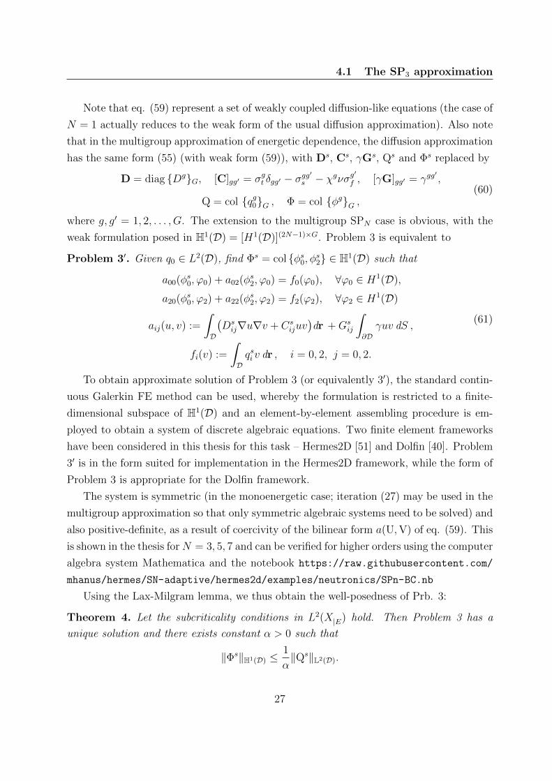
Note that eq. (59) represent a set of weakly coupled diffusion-like equations (the case of
N = 1 actually reduces to the weak form of the usual diffusion approximation). Also note
that in the multigroup approximation of energetic dependence, the diffusion approximation
has the same form (55) (with weak form (59)), with Ds, Cs, γGs, Qs and Φs replaced by
D = diag DgG, [C]gg′ = σgt δgg′ − σgg′
s − χgνσg′
f , [γG]gg′ = γgg′,
Q = col qg0G , Φ = col φgG ,(60)
where g, g′ = 1, 2, . . . , G. The extension to the multigroup SPN case is obvious, with the
weak formulation posed in H1(D) = [H1(D)](2N−1)×G. Problem 3 is equivalent to
Problem 3′. Given q0 ∈ L2(D), find Φs = col φs0, φs2 ∈ H1(D) such that
a00(φs0, ϕ0) + a02(φs2, ϕ0) = f0(ϕ0), ∀ϕ0 ∈ H1(D),
a20(φs0, ϕ2) + a22(φs2, ϕ2) = f2(ϕ2), ∀ϕ2 ∈ H1(D)
aij(u, v) :=
∫D
(Dsij∇u∇v + Cs
ijuv)dr +Gs
ij
∫∂Dγuv dS ,
fi(v) :=
∫Dqsi v dr , i = 0, 2, j = 0, 2.
(61)
To obtain approximate solution of Problem 3 (or equivalently 3′), the standard contin-
uous Galerkin FE method can be used, whereby the formulation is restricted to a finite-
dimensional subspace of H1(D) and an element-by-element assembling procedure is em-
ployed to obtain a system of discrete algebraic equations. Two finite element frameworks
have been considered in this thesis for this task – Hermes2D [51] and Dolfin [40]. Problem
3′ is in the form suited for implementation in the Hermes2D framework, while the form of
Problem 3 is appropriate for the Dolfin framework.
The system is symmetric (in the monoenergetic case; iteration (27) may be used in the
multigroup approximation so that only symmetric algebraic systems need to be solved) and
also positive-definite, as a result of coercivity of the bilinear form a(U,V) of eq. (59). This
is shown in the thesis forN = 3, 5, 7 and can be verified for higher orders using the computer
algebra system Mathematica and the notebook https://raw.githubusercontent.com/
mhanus/hermes/SN-adaptive/hermes2d/examples/neutronics/SPn-BC.nb
Using the Lax-Milgram lemma, we thus obtain the well-posedness of Prb. 3:
Theorem 4. Let the subcriticality conditions in L2(X|E) hold. Then Problem 3 has a
unique solution and there exists constant α > 0 such that
‖Φs‖H1(D) ≤1
α‖Qs‖L2(D).
27
5 The MCPN approximation
5 The MCPN approximation
Let us now return to the PN approximation. While it is possible to reduce the correspond-
ing set of equations (30) into a system of second-order partial differential equations, the
resulting set is rather complicated ([8, 45]) and in no way resembles the simple elliptic
system of the SPN approximation. This motivates the search for an alternative form of
the expansion (28) that would reveal some connection with the computationally attractive
SPN approximation. To illustrate one such possible choice and its consequences, we will
consider the monoenergetic NTE in the form
Ω · ∇ψ(r,Ω) + σt(r)ψ(r,Ω)
−∫S2
[σs(r,Ω ·Ω′) +
νσf (r)
4π
]ψ(r,Ω′) dΩ′ − q(r,Ω) = 0, (r,Ω) ∈ D × S2
(62)
and assume that ψ(r, ·) ∈ L2(S2).
5.1 Maxwell-Cartesian spherical harmonics
A general linear combination of tesseral harmonics of given degree n is called surface
spherical harmonic of degree n. As shown in [3], a surface spherical harmonic of degree n
can also be uniquely represented in a form of a special kind of Cartesian tensor.
We will denote a Cartesian tensor of rank n either by a blackboard letter (like A(n)) or
by superscribed (n) and subscribed sequence of n Greek letters indicating its 3n components
(each attaining value 1, 2, or 3, corresponding to Cartesian axes x, y, z, respectively) –
like A(2)αβ or A
(n)γ1...γn ; for vectors (rank-1 tensors), we will keep using conventional bold-face
letters. Einstein’s summation convention will be used whenever same indices appear in a
tensor expression written in component notation. When a tensor is invariant under any
permutation of its indices, it is called totally symmetric; contraction of two tensors of same
rank is a number A(n) ·B(n) := A(n)γ1...γnB
(n)γn...γ1 , contraction of a tensor A(n) in first index pair
is defined as A(n)ααγ3...γn and called trace in that index pair. Totally symmetric tensor whose
trace in any index pair vanishes is called totally symmetric traceless (abbr. TST). The
tensor product C(n+m) = A(n) ⊗ B(m) has components C(n+m)α1...αnβ1...βm
= A(n)α1...αnB
(m)β1...βm
and
the m-th power of a rank-n tensor is defined as A(n)⊗A(n)⊗ · · ·⊗A(n) (m-times). Finally,
we will consider the differential operator ∇ as a vector [ ∂∂x, ∂∂y, ∂∂z
]T , but keep writing ∇A(n)
for ∇⊗ A(n).
The paper [3] presents a systematic way of obtaining a TST tensor of any rank n whose
components are surface spherical harmonics of degree n in Cartesian frame of reference
28
5.2 MCPN approximation
as defined by Maxwell in [43, p. 160]. Specifically, Maxwell’s spherical harmonics based
on Cartesian axes can be obtained (up to a normalization constant) as components of
P(n)(Ω) = DΩn where D is the so-called detracer operator which projects a general totally
symmetric tensor of rank n into the space of TST tensors of rank n. We note that pro-
jection of P(n) along, say, z-axis (or any other because of the symmetry) yields (up to a
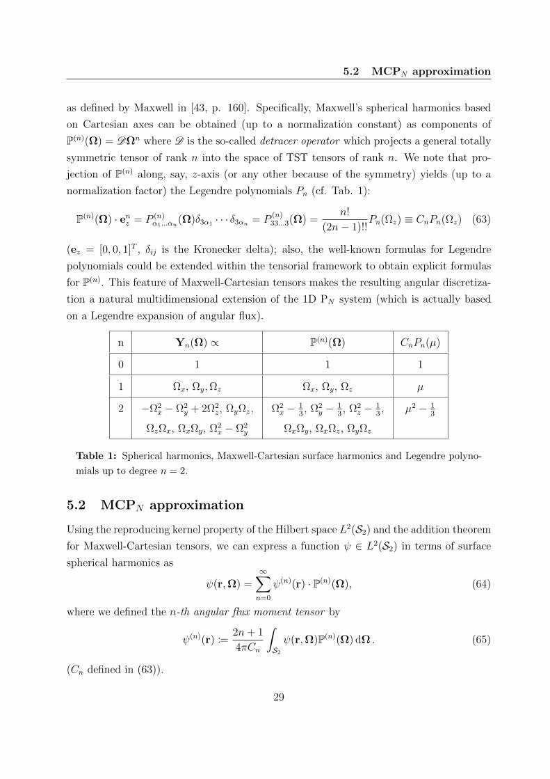
normalization factor) the Legendre polynomials Pn (cf. Tab. 1):
P(n)(Ω) · enz = P (n)α1...αn
(Ω)δ3α1 · · · δ3αn = P(n)33...3(Ω) =
n!
(2n− 1)!!Pn(Ωz) ≡ CnPn(Ωz) (63)
(ez = [0, 0, 1]T , δij is the Kronecker delta); also, the well-known formulas for Legendre
polynomials could be extended within the tensorial framework to obtain explicit formulas
for P(n). This feature of Maxwell-Cartesian tensors makes the resulting angular discretiza-
tion a natural multidimensional extension of the 1D PN system (which is actually based
on a Legendre expansion of angular flux).
n Yn(Ω) ∝ P(n)(Ω) CnPn(µ)
0 1 1 1
1 Ωx, Ωy,Ωz Ωx, Ωy, Ωz µ
2 −Ω2x − Ω2
y + 2Ω2z, ΩyΩz,
ΩzΩx, ΩxΩy, Ω2x − Ω2
y
Ω2x − 1
3, Ω2
y − 13, Ω2
z − 13,
ΩxΩy, ΩxΩz, ΩyΩz
µ2 − 13
Table 1: Spherical harmonics, Maxwell-Cartesian surface harmonics and Legendre polyno-
mials up to degree n = 2.
5.2 MCPN approximation
Using the reproducing kernel property of the Hilbert space L2(S2) and the addition theorem
for Maxwell-Cartesian tensors, we can express a function ψ ∈ L2(S2) in terms of surface
spherical harmonics as
ψ(r,Ω) =∞∑n=0
ψ(n)(r) · P(n)(Ω), (64)
where we defined the n-th angular flux moment tensor by
ψ(n)(r) :=2n+ 1
4πCn
∫S2ψ(r,Ω)P(n)(Ω) dΩ . (65)
(Cn defined in (63)).
29
5 The MCPN approximation
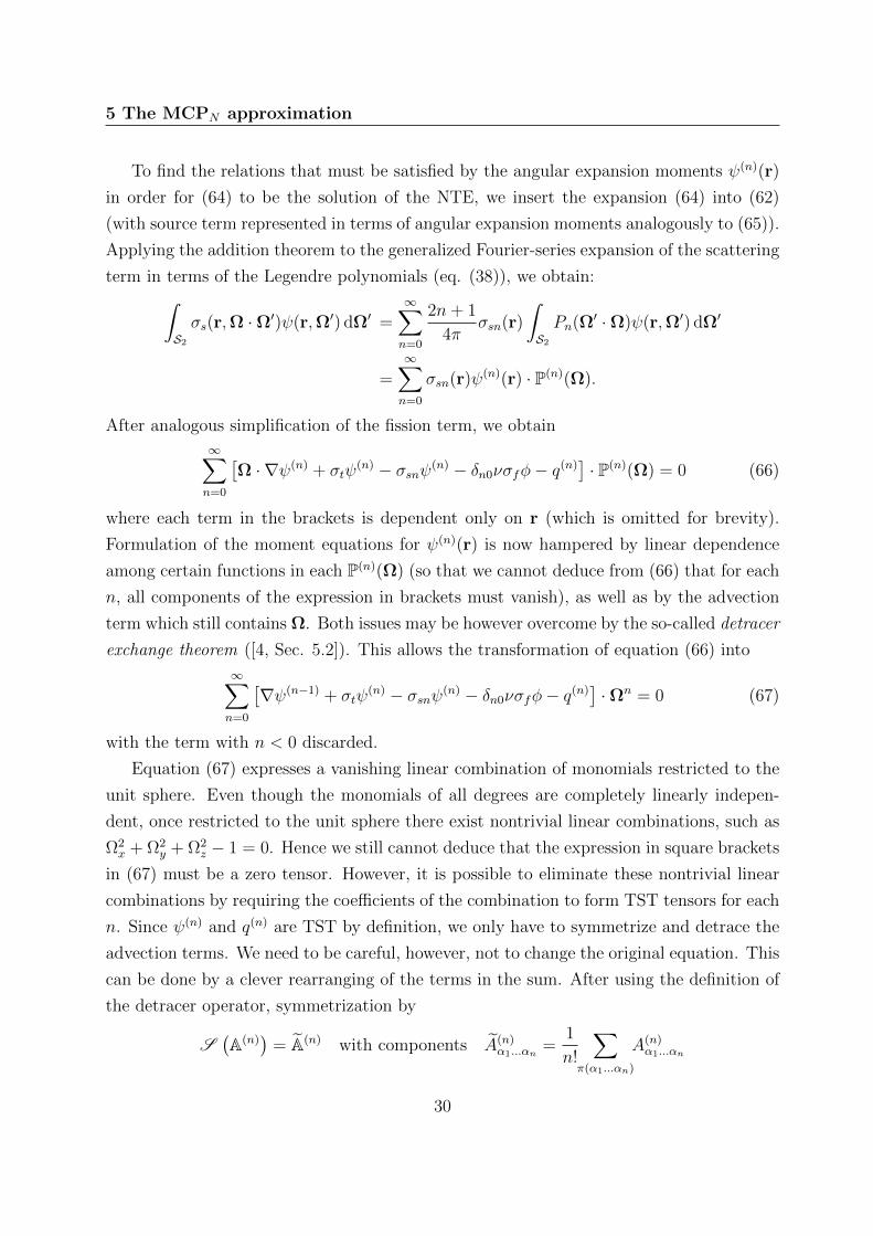
To find the relations that must be satisfied by the angular expansion moments ψ(n)(r)
in order for (64) to be the solution of the NTE, we insert the expansion (64) into (62)
(with source term represented in terms of angular expansion moments analogously to (65)).
Applying the addition theorem to the generalized Fourier-series expansion of the scattering
term in terms of the Legendre polynomials (eq. (38)), we obtain:∫S2σs(r,Ω ·Ω′)ψ(r,Ω′) dΩ′ =
∞∑n=0
2n+ 1
4πσsn(r)
∫S2Pn(Ω′ ·Ω)ψ(r,Ω′) dΩ′
=∞∑n=0
σsn(r)ψ(n)(r) · P(n)(Ω).
After analogous simplification of the fission term, we obtain
∞∑n=0
[Ω · ∇ψ(n) + σtψ
(n) − σsnψ(n) − δn0νσfφ− q(n)]· P(n)(Ω) = 0 (66)
where each term in the brackets is dependent only on r (which is omitted for brevity).
Formulation of the moment equations for ψ(n)(r) is now hampered by linear dependence
among certain functions in each P(n)(Ω) (so that we cannot deduce from (66) that for each
n, all components of the expression in brackets must vanish), as well as by the advection
term which still contains Ω. Both issues may be however overcome by the so-called detracer
exchange theorem ([4, Sec. 5.2]). This allows the transformation of equation (66) into
∞∑n=0
[∇ψ(n−1) + σtψ
(n) − σsnψ(n) − δn0νσfφ− q(n)]·Ωn = 0 (67)
with the term with n < 0 discarded.
Equation (67) expresses a vanishing linear combination of monomials restricted to the
unit sphere. Even though the monomials of all degrees are completely linearly indepen-
dent, once restricted to the unit sphere there exist nontrivial linear combinations, such as
Ω2x + Ω2
y + Ω2z − 1 = 0. Hence we still cannot deduce that the expression in square brackets
in (67) must be a zero tensor. However, it is possible to eliminate these nontrivial linear
combinations by requiring the coefficients of the combination to form TST tensors for each
n. Since ψ(n) and q(n) are TST by definition, we only have to symmetrize and detrace the
advection terms. We need to be careful, however, not to change the original equation. This
can be done by a clever rearranging of the terms in the sum. After using the definition of
the detracer operator, symmetrization by
S(A(n)
)= A(n) with components A(n)
α1...αn=
1
n!
∑π(α1...αn)
A(n)α1...αn
30
5.3 The MCP3 system
(where the sum is over all permutations of the tensor indices) and regrouping the sum by
Ωn, we arrive at the final equation (with Σn := σtψ(n) − σsnψ(n) − δn0νσf )
∞∑n=0
S
(∇ψ(n−1) − n− 1
2n− 1I⊗∇ · ψ(n−1)
)+
n+ 1
2n+ 3∇ · ψ(n+1) + Σnψ
(n) − q(n)
·Ωn = 0,
(68)
which implies that each component of the TST coefficient tensor of rank n in curly brackets
must vanish.
5.3 The MCP3 system
We can see that the MCP1 set is equivalent to the P1 set. For N ≥ 3, we have to take
into account the definition of the moments as traceless totally symmetric tensors. If we
considered general symmetric moment tensors ψ(2), ψ(3), etc., we would obtain more linearly
independent equations than in the corresponding PN set. However, by restricting to TST
tensors (by applying the detracer operator on the moments), we obtain the same number
of linearly independent equations in the set (68) as in the PN set.
Moreover, the MCPN equations can be written in the form of (30):
AxMCPN
∂Φ
∂x+ Ay
MCPN
∂Φ
∂y+ Az
MCPN
∂Φ
∂z+[σtI−KMCPN
]Φ = Q, (69)
where Φ and Q now contain the different MCPN moments.
In Appendix D of the thesis, we showed that the advection matrices AxMCP3
, AyMCP3
,
AzMCP3
have the same eigenvalues, which are moreover equal to those of the advection
matrices of the P3 approximation (only the multiplicity of the zero eigenvalue is greater,
reflecting the linear dependence between the MCP3 equations). The paper [3] shows how to
systematically select linearly independent subsets of the TST tensors, which could be used
to actually solve the MCP3 equations. However, we stress that this is not our intention
since this would be no easier than solving the ordinary P3] equations.
Rather, by exploiting the symmetric and traceless structure of the MCP3 tensors and
using some algebra, we find out that in a homogeneous region, the MCP3 equations imply
that the scalar flux is governed by the following fourth-order PDE:
3
35Σ3∇4φ−
(11
21
Σ0
Σ2+
1
3Σ
)∇2φ+ Σ0φ = q − 11
21Σ2∇2q. (70)
31
5 The MCPN approximation
(where further isotropic scattering and sources were assumed for simplicity). Moreover,
this equation may be split into two coupled diffusion-like equations
− 1
3Σ∇2φ+
55
27Σ0φ−
70
27Σθ =
55
27q,
− 1
3Σ∇2θ +
35
27Σθ − 14
27Σ0φ = −14
27q.
(71)
which are equivalent to the SP3 equations (55), (56) (Sec. 5.4.2 of the thesis).
In an infinite homogeneous medium, these equations may be solved for scalar flux
φ equivalent to one that would be obtained from the full set of 16 independent MCP3
equations. Boundary and interface conditions need to be derived for solving problems in
bounded and/or heterogeneous domains. Because of the formal equivalence with the SP3
continuity of
φ, θ,1
Σ
∂φ
∂n,
1
Σ
∂θ
∂n
and boundary conditions analogous to those of the SP3 model suggest themselves as a first
approximation. However, these conditions are obviously not in general compatible with
the MCP3 model anymore.
A concrete set of interface conditions compatible with both the equations for angular
flux moments and the diffusion-like equations has been presented in a rather puzzling
paper [56] (see also commentary in [18, Sec. 5.2]). Starting from the even-parity NTE, the
author “derived” equation (70) and equations (71), as well as conditions for the even-parity
tensorial moments and the unknowns of the diffusion-like equations – all on a half-page
space.
Even though the excessive brevity of the paper prevented further study and practical use
of these equations and conditions, the equivalence of the equations to those systematically
derived in previous subsections may motivate the search for the additional conditions in
the same form as in [56]. The approach used in [56] requires to express the second-
order moment tensor ψ(2) in terms of φ (which constitutes another puzzling equation,
eq. (7), in the paper). In a preliminary investigation, we were able to derive [56, Eq.
(7)] as a scalar part of the scalar-vector-tensor decomposition of ψ(2) ([13]), which is the
complete representation of the tensor under the assumption of ψ(1) and ψ(3) being curl-free
(conservative). This indicates one direction that may be taken in the quest for complete
understanding of Selengut’s paper (and formulating a practical way of obtaining PN scalar
flux from solving much smaller system of elliptic equations).
32
6 Neutronics modules
6 Neutronics modules
6.1 Hermes2D modules
As we have seen in Sec. 3, the various transport approximations lead to coupled systems
of differential equations with finite element approximations formulated on product spaces.
In order to implement these models into a practical solution method, it is thus necessary
to appropriately deal with the coupling of variables.
The C++ finite element library Hermes2D is particularly suited for this type of prob-
lems thanks to its original multimesh assembling approach [50]. We extended the multimesh
assembling to the case of discontinuous approximations, allowing the implementation of
the discontinuous Galerkin method and particularly the SN method. Together with the
multigroup SPN module (up to N = 9; using the Mathematica script referred to in Sec. 4
allows for simple extension to higher orders), these modules simplify the definition of stan-
dard neutronics problems (both fixed source and eigenvalue) and support experimentation
with other transport approximations7.
The multimesh assembling is also an important ingredient for efficient hp-adaptivity,
as it allows each solution component to be represented on its own approximation space
(with its own underlying mesh and distribution of local approximation orders), based on
hierarchical polynomial basis (with additional enforcement of conformity for continuous
Galerkin approximation). The adaptivity itself is driven by local error estimates based on
comparing two solutions of different approximation orders, which allows to determine the
whole shape of the approximation error over each element and use it to determine the best
refinement candidate that decreases the total approximation error for the lowest number of
added degrees of freedom (DOF). In this way, various candidate combinations of element
refinements and approximation order changes can be compared, taking into account all
elements of all meshes (i.e. the coupling of the solved PDE system).
For solving the criticality eigenvalue problems of type (26), the (inexact) inverse itera-
tion has been implemented according to paper [26]. It supports both fixed and Rayleigh
quotient shifting and exact and inexact solves (with fixed or decreasing tolerance during
the course of the eigenvalue iteration) of the associated linear system in the i-th iteration.
7The multigroup diffusion framework is available in the master branch of current Hermes2D release; the
SPN version with various examples can be downloaded from https://github.com/mhanus/hermes/
tree/neutronics-master. The development version intended mainly for testing the SN module
(including additional SN examples) is available from https://github.com/mhanus/hermes/tree/
SN-adaptive.
33
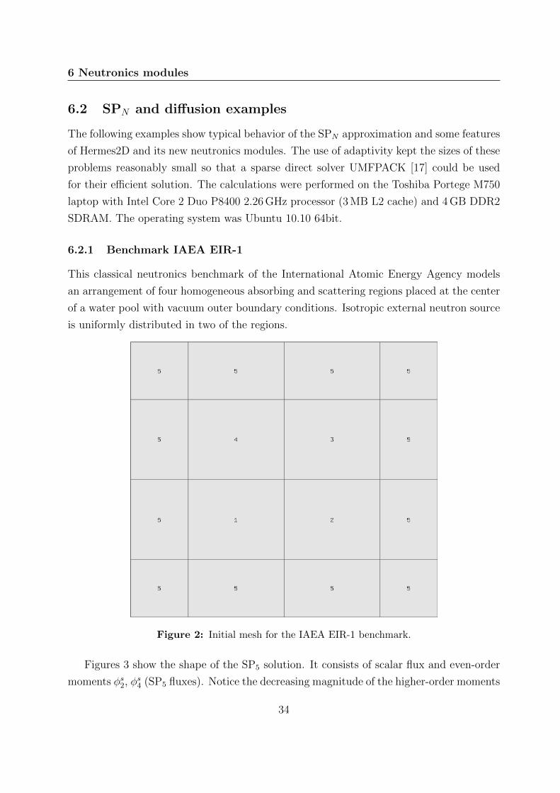
6 Neutronics modules
6.2 SPN and diffusion examples
The following examples show typical behavior of the SPN approximation and some features
of Hermes2D and its new neutronics modules. The use of adaptivity kept the sizes of these
problems reasonably small so that a sparse direct solver UMFPACK [17] could be used
for their efficient solution. The calculations were performed on the Toshiba Portege M750
laptop with Intel Core 2 Duo P8400 2.26 GHz processor (3 MB L2 cache) and 4 GB DDR2
SDRAM. The operating system was Ubuntu 10.10 64bit.
6.2.1 Benchmark IAEA EIR-1
This classical neutronics benchmark of the International Atomic Energy Agency models
an arrangement of four homogeneous absorbing and scattering regions placed at the center
of a water pool with vacuum outer boundary conditions. Isotropic external neutron source
is uniformly distributed in two of the regions.
Figure 2: Initial mesh for the IAEA EIR-1 benchmark.
Figures 3 show the shape of the SP5 solution. It consists of scalar flux and even-order
moments φs2, φs4 (SP5 fluxes). Notice the decreasing magnitude of the higher-order moments
34
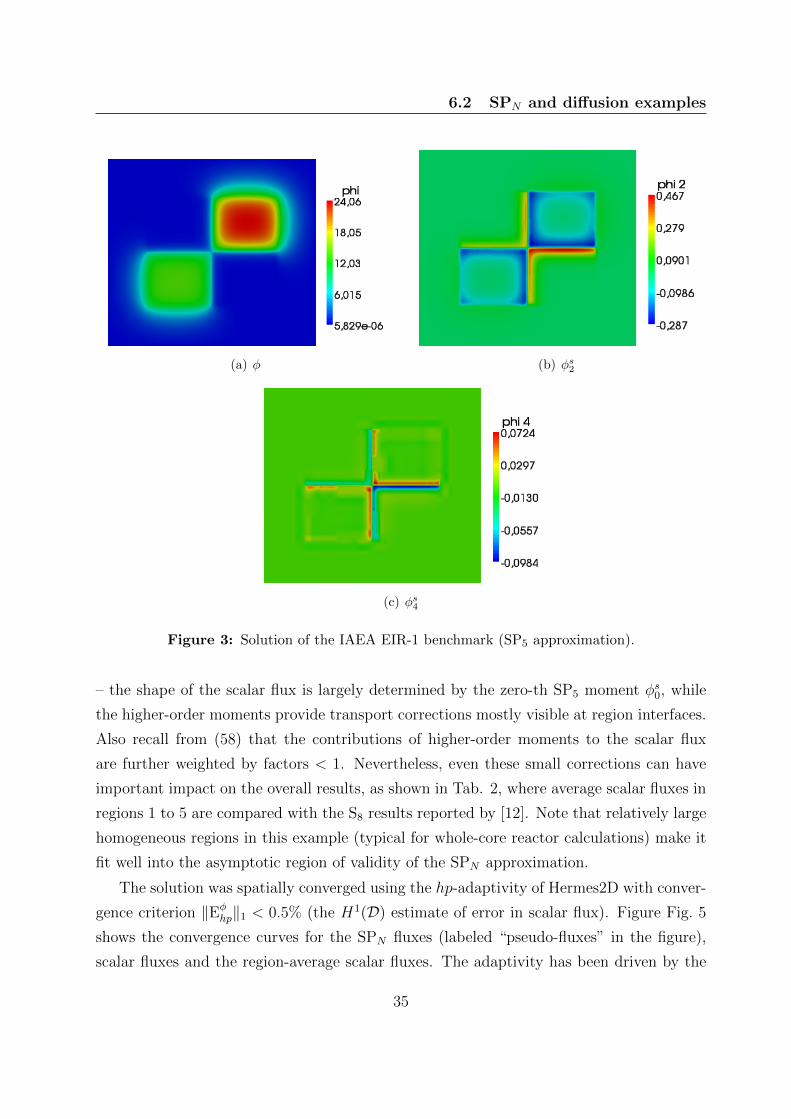
6.2 SPN and diffusion examples
(a) φ (b) φs2
(c) φs4
Figure 3: Solution of the IAEA EIR-1 benchmark (SP5 approximation).
– the shape of the scalar flux is largely determined by the zero-th SP5 moment φs0, while
the higher-order moments provide transport corrections mostly visible at region interfaces.
Also recall from (58) that the contributions of higher-order moments to the scalar flux
are further weighted by factors < 1. Nevertheless, even these small corrections can have
important impact on the overall results, as shown in Tab. 2, where average scalar fluxes in
regions 1 to 5 are compared with the S8 results reported by [12]. Note that relatively large
homogeneous regions in this example (typical for whole-core reactor calculations) make it
fit well into the asymptotic region of validity of the SPN approximation.
The solution was spatially converged using the hp-adaptivity of Hermes2D with conver-
gence criterion ‖Eφhp‖1 < 0.5% (the H1(D) estimate of error in scalar flux). Figure Fig. 5
shows the convergence curves for the SPN fluxes (labeled “pseudo-fluxes” in the figure),
scalar fluxes and the region-average scalar fluxes. The adaptivity has been driven by the
35
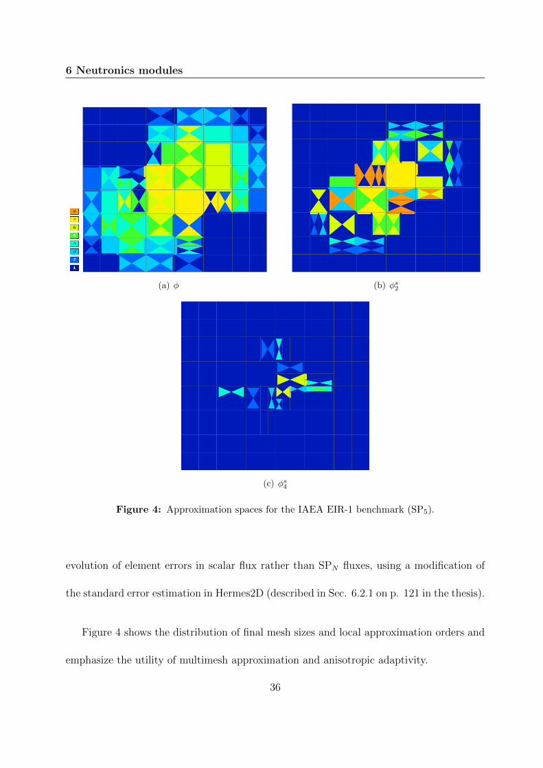
6 Neutronics modules
(a) φ (b) φs2
(c) φs4
Figure 4: Approximation spaces for the IAEA EIR-1 benchmark (SP5).
evolution of element errors in scalar flux rather than SPN fluxes, using a modification of
the standard error estimation in Hermes2D (described in Sec. 6.2.1 on p. 121 in the thesis).
Figure 4 shows the distribution of final mesh sizes and local approximation orders and
emphasize the utility of multimesh approximation and anisotropic adaptivity.
36
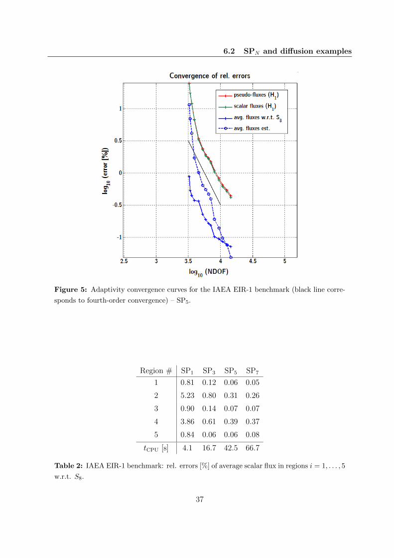
6.2 SPN and diffusion examples
Figure 5: Adaptivity convergence curves for the IAEA EIR-1 benchmark (black line corre-
sponds to fourth-order convergence) – SP5.
Region # SP1 SP3 SP5 SP7
1 0.81 0.12 0.06 0.05
2 5.23 0.80 0.31 0.26
3 0.90 0.14 0.07 0.07
4 3.86 0.61 0.39 0.37
5 0.84 0.06 0.06 0.08
tCPU [s] 4.1 16.7 42.5 66.7
Table 2: IAEA EIR-1 benchmark: rel. errors [%] of average scalar flux in regions i = 1, . . . , 5
w.r.t. S8.
37
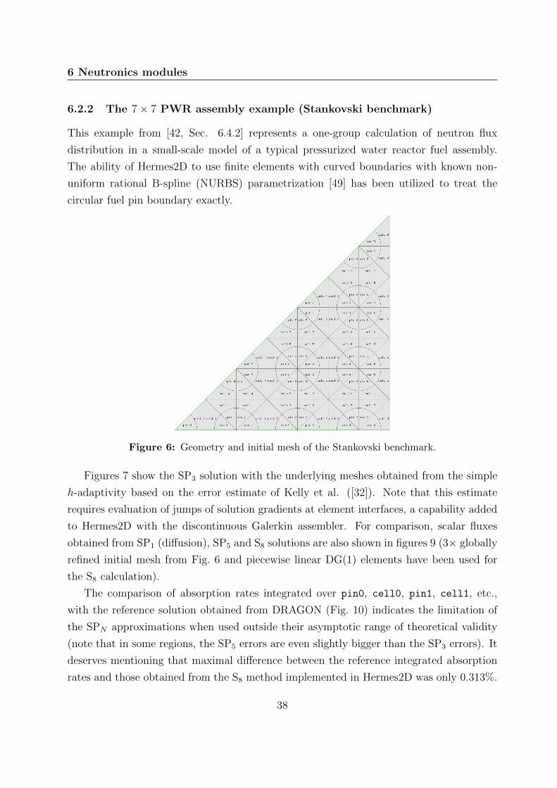
6 Neutronics modules
6.2.2 The 7× 7 PWR assembly example (Stankovski benchmark)
This example from [42, Sec. 6.4.2] represents a one-group calculation of neutron flux
distribution in a small-scale model of a typical pressurized water reactor fuel assembly.
The ability of Hermes2D to use finite elements with curved boundaries with known non-
uniform rational B-spline (NURBS) parametrization [49] has been utilized to treat the
circular fuel pin boundary exactly.
Figure 6: Geometry and initial mesh of the Stankovski benchmark.
Figures 7 show the SP3 solution with the underlying meshes obtained from the simple
h-adaptivity based on the error estimate of Kelly et al. ([32]). Note that this estimate
requires evaluation of jumps of solution gradients at element interfaces, a capability added
to Hermes2D with the discontinuous Galerkin assembler. For comparison, scalar fluxes
obtained from SP1 (diffusion), SP5 and S8 solutions are also shown in figures 9 (3× globally
refined initial mesh from Fig. 6 and piecewise linear DG(1) elements have been used for
the S8 calculation).
The comparison of absorption rates integrated over pin0, cell0, pin1, cell1, etc.,
with the reference solution obtained from DRAGON (Fig. 10) indicates the limitation of
the SPN approximations when used outside their asymptotic range of theoretical validity
(note that in some regions, the SP5 errors are even slightly bigger than the SP3 errors). It
deserves mentioning that maximal difference between the reference integrated absorption
rates and those obtained from the S8 method implemented in Hermes2D was only 0.313%.
38
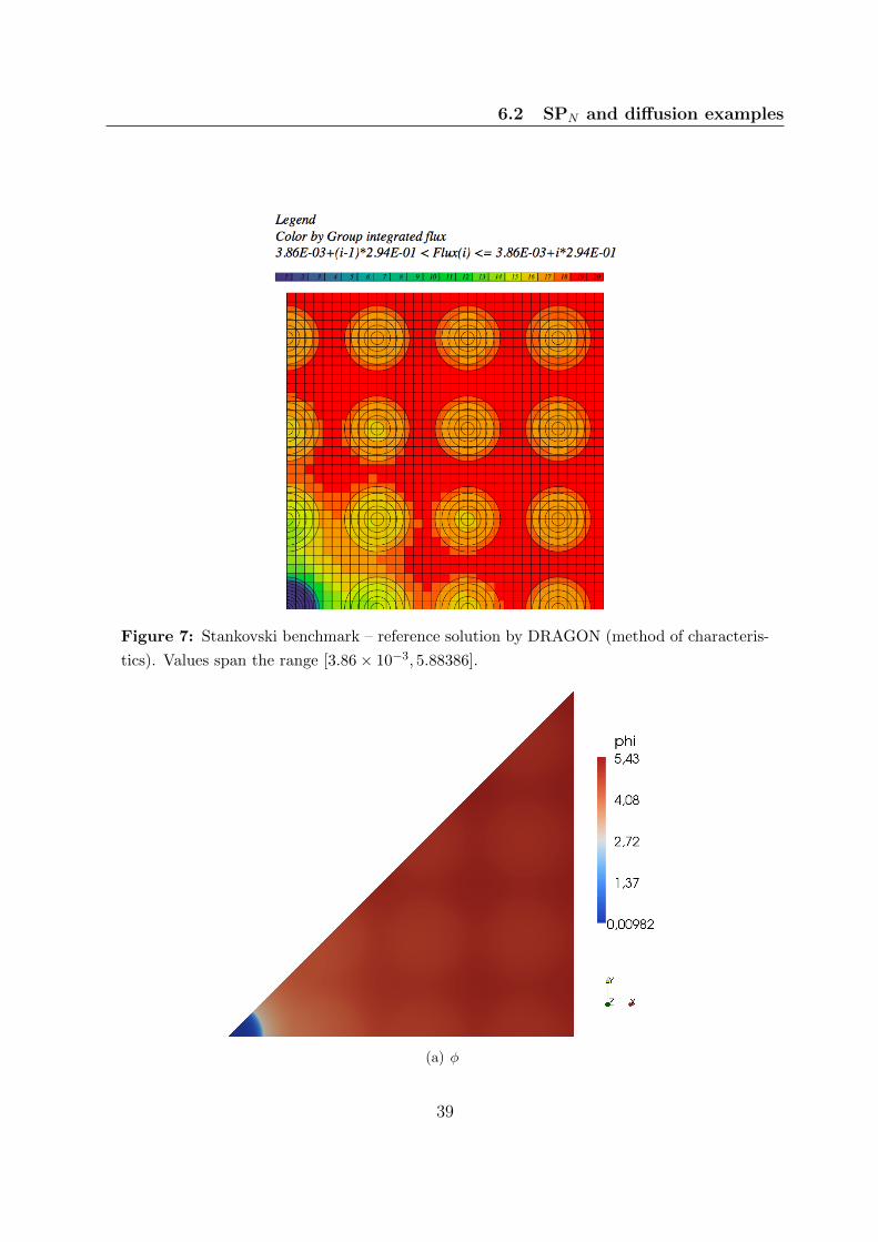
6.2 SPN and diffusion examples
Figure 7: Stankovski benchmark – reference solution by DRAGON (method of characteris-
tics). Values span the range [3.86× 10⁻³, 5.88386].
(a) φ
39
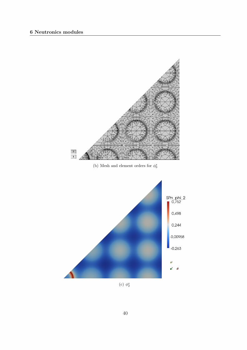
6 Neutronics modules
(b) Mesh and element orders for φs0
(c) φs2
40
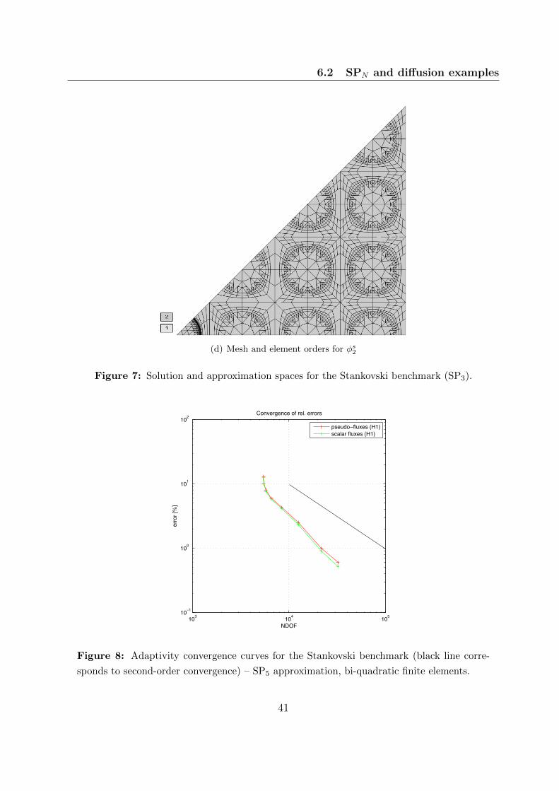
6.2 SPN and diffusion examples
(d) Mesh and element orders for φs2
Figure 7: Solution and approximation spaces for the Stankovski benchmark (SP3).
103 104 10510−1
100
101
102Convergence of rel. errors
NDOF
erro
r [%
]
pseudo−fluxes (H1)scalar fluxes (H1)
Figure 8: Adaptivity convergence curves for the Stankovski benchmark (black line corre-
sponds to second-order convergence) – SP5 approximation, bi-quadratic finite elements.
41
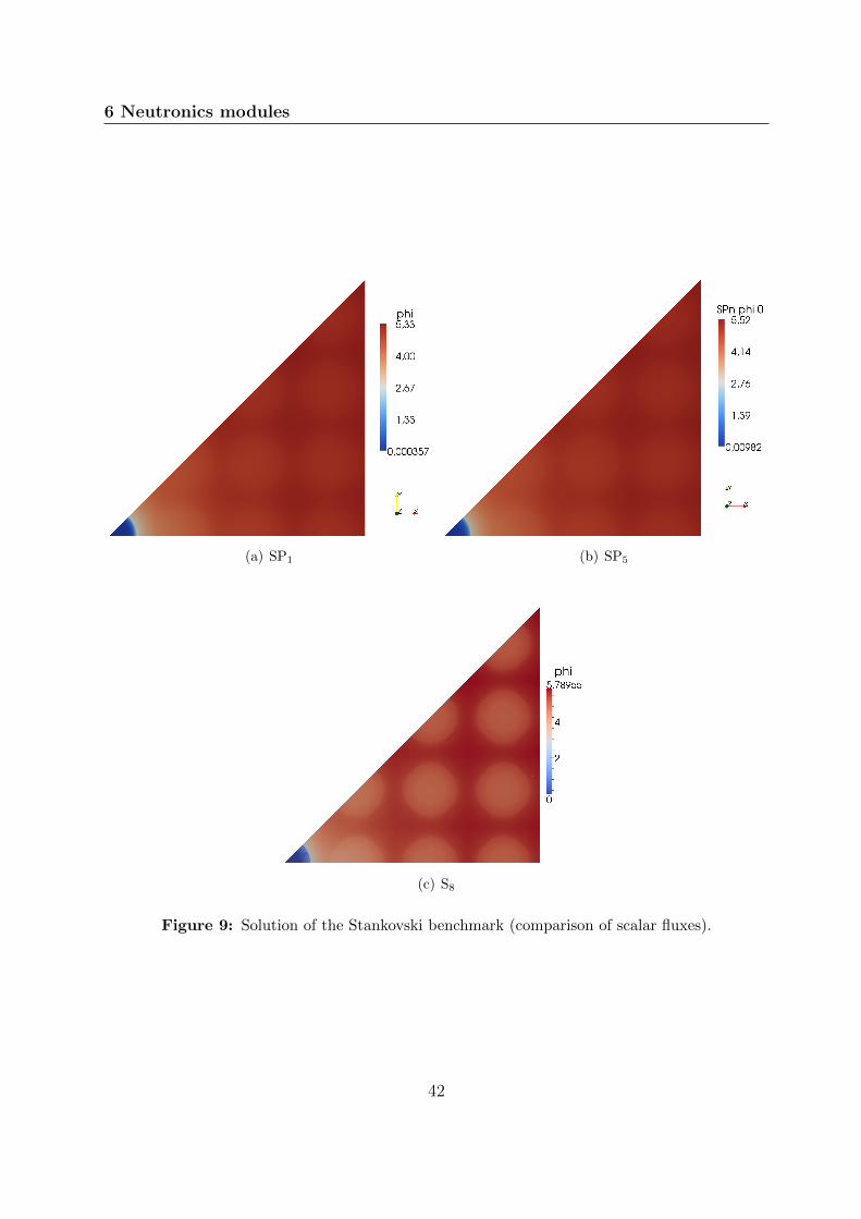
6 Neutronics modules
(a) SP1 (b) SP5
(c) S8
Figure 9: Solution of the Stankovski benchmark (comparison of scalar fluxes).
42
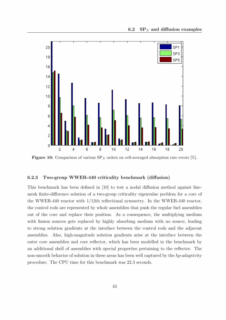
6.2 SPN and diffusion examples
Figure 10: Comparison of various SPN orders on cell-averaged absorption rate errors [%].
6.2.3 Two-group WWER-440 criticality benchmark (diffusion)
This benchmark has been defined in [10] to test a nodal diffusion method against fine-
mesh finite-difference solution of a two-group criticality eigenvalue problem for a core of
the WWER-440 reactor with 1/12th reflectional symmetry. In the WWER-440 reactor,
the control rods are represented by whole assemblies that push the regular fuel assemblies
out of the core and replace their position. As a consequence, the multiplying medium
with fission sources gets replaced by highly absorbing medium with no source, leading
to strong solution gradients at the interface between the control rods and the adjacent
assemblies. Also, high-magnitude solution gradients arise at the interface between the
outer core assemblies and core reflector, which has been modelled in the benchmark by
an additional shell of assemblies with special properties pertaining to the reflector. The
non-smooth behavior of solution in these areas has been well captured by the hp-adaptivity
procedure. The CPU time for this benchmark was 22.3 seconds.
43
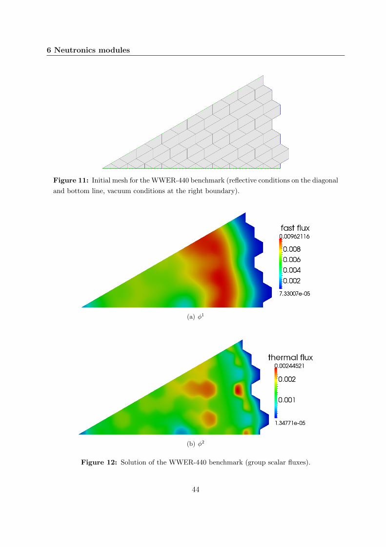
6 Neutronics modules
Figure 11: Initial mesh for the WWER-440 benchmark (reflective conditions on the diagonal
and bottom line, vacuum conditions at the right boundary).
(a) φ1
(b) φ2
Figure 12: Solution of the WWER-440 benchmark (group scalar fluxes).
44
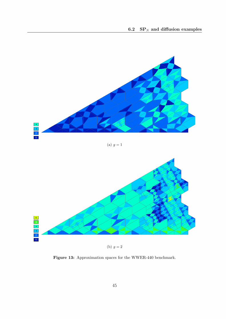
6.2 SPN and diffusion examples
(a) g = 1
(b) g = 2
Figure 13: Approximation spaces for the WWER-440 benchmark.
45
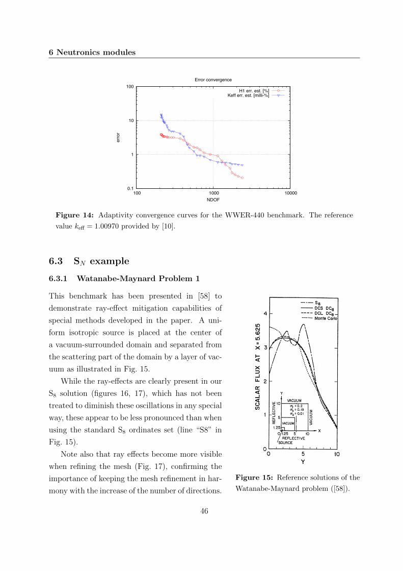
6 Neutronics modules
0.1
1
10
100
100 1000 10000
erro
r
NDOF
Error convergence
H1 err. est. [%]Keff err. est. [milli-%]
Figure 14: Adaptivity convergence curves for the WWER-440 benchmark. The reference
value keff = 1.00970 provided by [10].
6.3 SN example
6.3.1 Watanabe-Maynard Problem 1
Figure 15: Reference solutions of the
Watanabe-Maynard problem ([58]).
This benchmark has been presented in [58] to
demonstrate ray-effect mitigation capabilities of
special methods developed in the paper. A uni-
form isotropic source is placed at the center of
a vacuum-surrounded domain and separated from
the scattering part of the domain by a layer of vac-
uum as illustrated in Fig. 15.
While the ray-effects are clearly present in our
S8 solution (figures 16, 17), which has not been
treated to diminish these oscillations in any special
way, these appear to be less pronounced than when
using the standard S8 ordinates set (line “S8” in
Fig. 15).
Note also that ray effects become more visible
when refining the mesh (Fig. 17), confirming the
importance of keeping the mesh refinement in har-
mony with the increase of the number of directions.
46
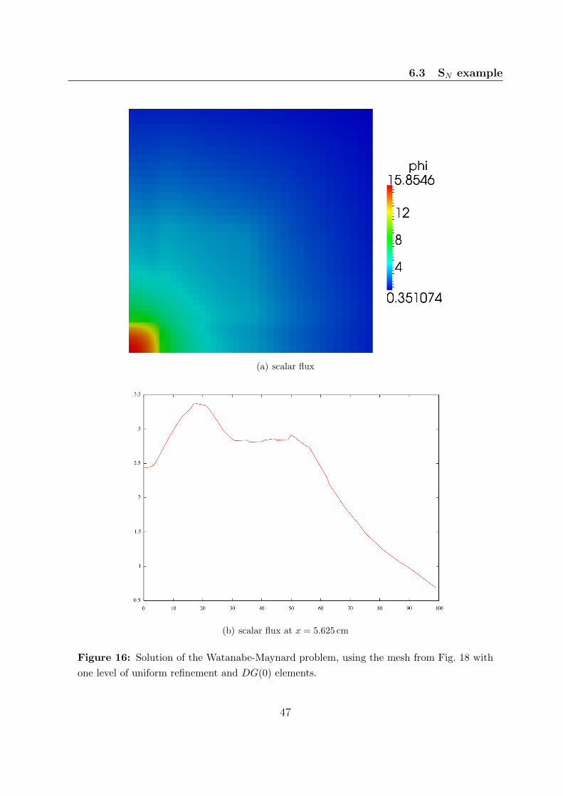
6.3 SN example
(a) scalar flux
(b) scalar flux at x = 5.625 cm
Figure 16: Solution of the Watanabe-Maynard problem, using the mesh from Fig. 18 with
one level of uniform refinement and DG(0) elements.
47
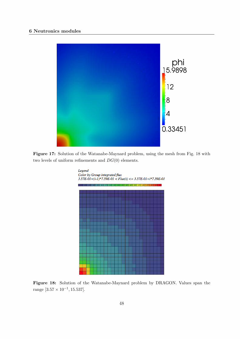
6 Neutronics modules
Figure 17: Solution of the Watanabe-Maynard problem, using the mesh from Fig. 18 with
two levels of uniform refinements and DG(0) elements.
Figure 18: Solution of the Watanabe-Maynard problem by DRAGON. Values span the
range [3.57× 10⁻¹, 15.537].
48
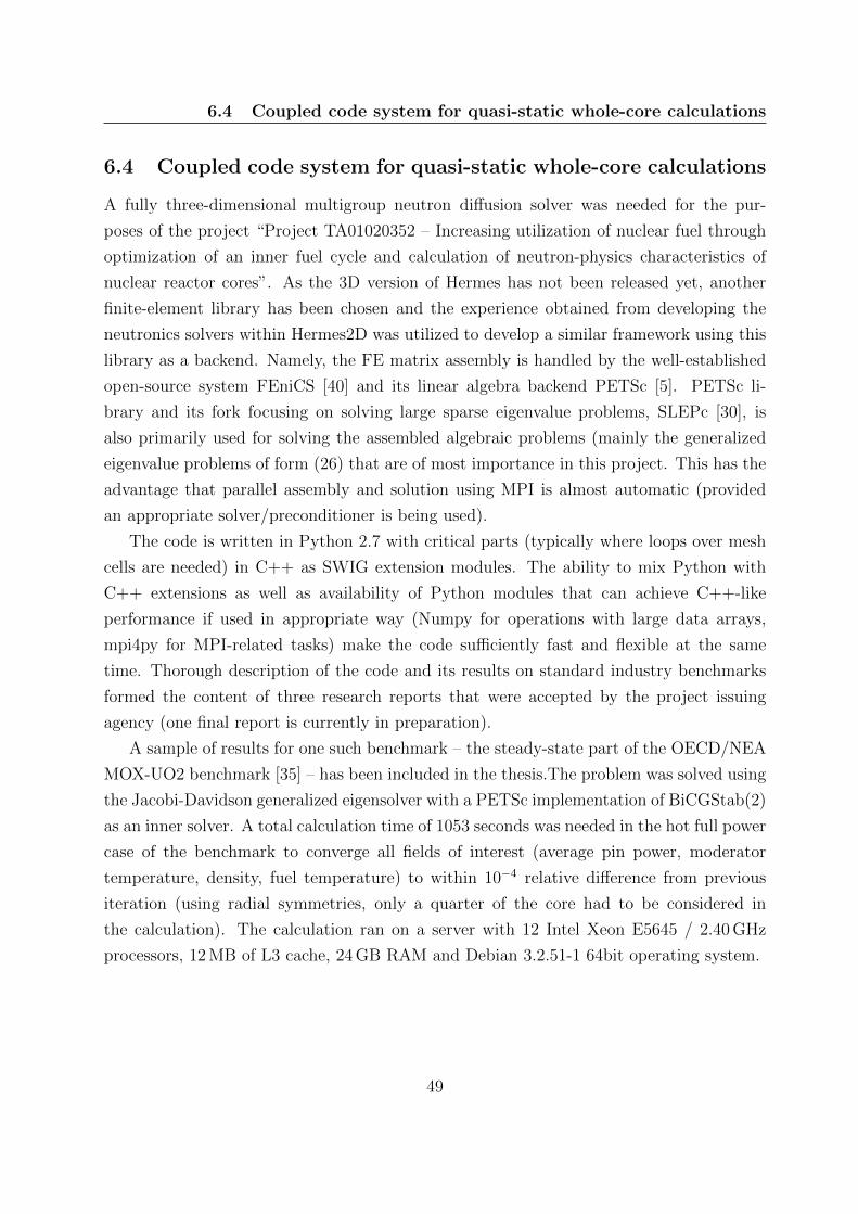
6.4 Coupled code system for quasi-static whole-core calculations
6.4 Coupled code system for quasi-static whole-core calculations
A fully three-dimensional multigroup neutron diffusion solver was needed for the pur-
poses of the project “Project TA01020352 – Increasing utilization of nuclear fuel through
optimization of an inner fuel cycle and calculation of neutron-physics characteristics of
nuclear reactor cores”. As the 3D version of Hermes has not been released yet, another
finite-element library has been chosen and the experience obtained from developing the
neutronics solvers within Hermes2D was utilized to develop a similar framework using this
library as a backend. Namely, the FE matrix assembly is handled by the well-established
open-source system FEniCS [40] and its linear algebra backend PETSc [5]. PETSc li-
brary and its fork focusing on solving large sparse eigenvalue problems, SLEPc [30], is
also primarily used for solving the assembled algebraic problems (mainly the generalized
eigenvalue problems of form (26) that are of most importance in this project. This has the
advantage that parallel assembly and solution using MPI is almost automatic (provided
an appropriate solver/preconditioner is being used).
The code is written in Python 2.7 with critical parts (typically where loops over mesh
cells are needed) in C++ as SWIG extension modules. The ability to mix Python with
C++ extensions as well as availability of Python modules that can achieve C++-like
performance if used in appropriate way (Numpy for operations with large data arrays,
mpi4py for MPI-related tasks) make the code sufficiently fast and flexible at the same
time. Thorough description of the code and its results on standard industry benchmarks
formed the content of three research reports that were accepted by the project issuing
agency (one final report is currently in preparation).
A sample of results for one such benchmark – the steady-state part of the OECD/NEA
MOX-UO2 benchmark [35] – has been included in the thesis.The problem was solved using
the Jacobi-Davidson generalized eigensolver with a PETSc implementation of BiCGStab(2)
as an inner solver. A total calculation time of 1053 seconds was needed in the hot full power
case of the benchmark to converge all fields of interest (average pin power, moderator
temperature, density, fuel temperature) to within 10−4 relative difference from previous
iteration (using radial symmetries, only a quarter of the core had to be considered in
the calculation). The calculation ran on a server with 12 Intel Xeon E5645 / 2.40 GHz
processors, 12 MB of L3 cache, 24 GB RAM and Debian 3.2.51-1 64bit operating system.
49
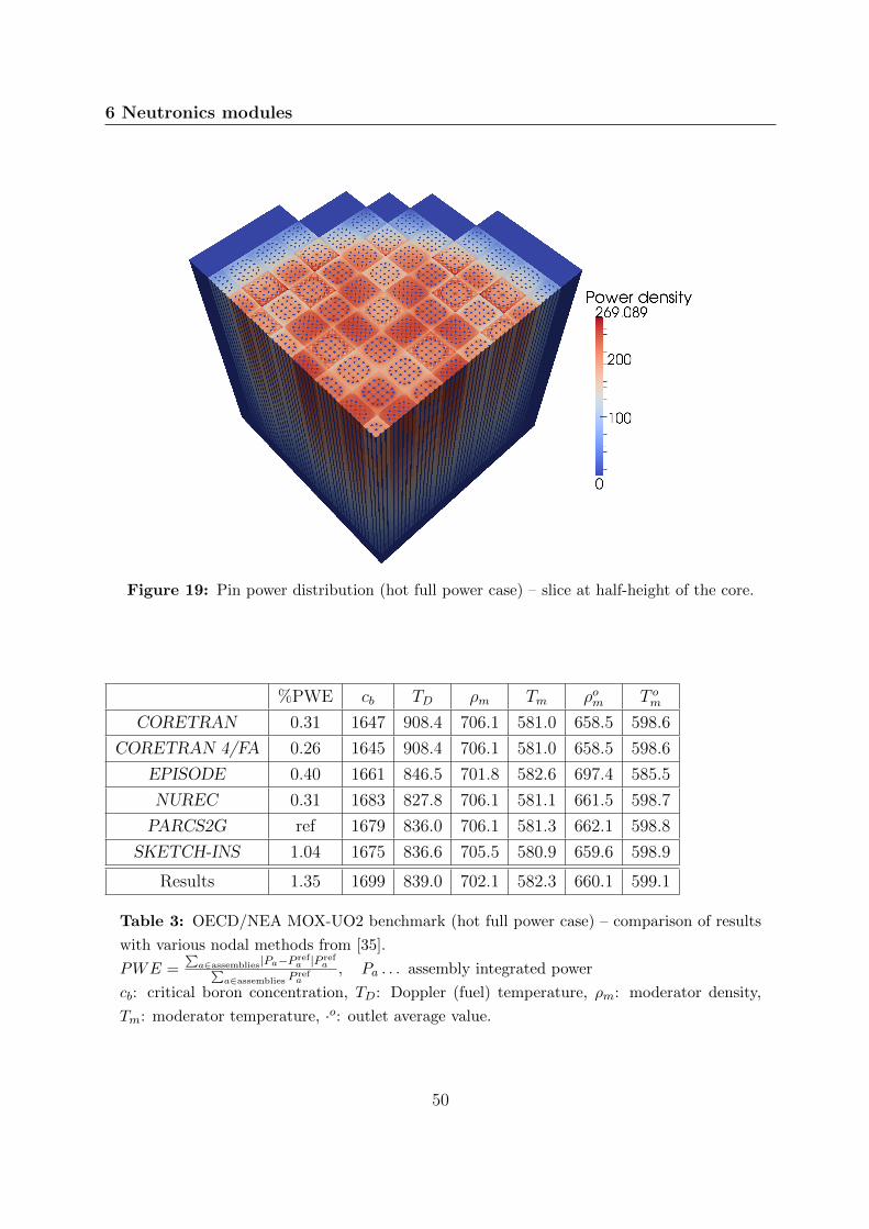
6 Neutronics modules
Figure 19: Pin power distribution (hot full power case) – slice at half-height of the core.
%PWE cb TD ρm Tm ρom T omCORETRAN 0.31 1647 908.4 706.1 581.0 658.5 598.6
CORETRAN 4/FA 0.26 1645 908.4 706.1 581.0 658.5 598.6
EPISODE 0.40 1661 846.5 701.8 582.6 697.4 585.5
NUREC 0.31 1683 827.8 706.1 581.1 661.5 598.7
PARCS2G ref 1679 836.0 706.1 581.3 662.1 598.8
SKETCH-INS 1.04 1675 836.6 705.5 580.9 659.6 598.9
Results 1.35 1699 839.0 702.1 582.3 660.1 599.1
Table 3: OECD/NEA MOX-UO2 benchmark (hot full power case) – comparison of results
with various nodal methods from [35].
PWE =∑
a∈assemblies|Pa−P refa |P ref
a∑a∈assemblies P
refa
, Pa . . . assembly integrated power
cb: critical boron concentration, TD: Doppler (fuel) temperature, ρm: moderator density,
Tm: moderator temperature, ·o: outlet average value.
50
7 Summary
7 Summary
The thesis is devoted to mathematical and numerical modeling of neutron transport. We
started by reviewing the fundamental mathematical model and some well-known approx-
imation techniques. The section on classical discretization of energetic dependence – the
multigroup method was followed by the description of two most widely used methods for
approximating angular dependence (the SN and PN methods). We demonstrated how these
two methods – well known for a long time, but typically presented independently of each
other – can be described using a single abstract mathematical framework – as a projection
of the transport equation onto a suitable Hilbert space. Viewing the SN approximation as
a subspace projection makes the properties of the continuous NTE directly translate to the
approximate method. As a particular example, we outlined how this fact could be used to
prove convergence of the basic iterative method for actual solution of the SN equations –
the source iteration.
The part devoted to angular approximation methods was concluded by introducing a
concrete angular quadrature set for the SN approximation, satisfying various requirements
uncovered during the description of the approximation. This quadrature set was later used
in an actual computer code for solving the SN equations. In order to obtain this final
neutron transport solver, the spatial dependence in the NTE had to be discretized. For
this purpose, a general discontinuous Galerkin method was applied to the SN equations
to obtain the weak formulation in a form suitable for implementing into common finite
element libraries.
Then we turned our attention to the PN approximation. We recalled the diffusion equa-
tion, a standard tool for whole-core nuclear reactor calculations that can be obtained from
the lowest order P1 approximation. Unlike the SN approximation, standard continuous
Galerkin finite elements can be used for discretizing the diffusion equation and a symmet-
ric and positive definite system of algebraic equations is obtained by the procedure in the
monoenergetic case. This allows to use mature methods for solving such algebraic systems,
like the conjugate gradient method preconditioned by algebraic multigrid.
Some recent nuclear reactor problems involving higher amount of material and geo-
metric heterogeneity, where diffusion no longer provides an adequate approximation and
using SN approximation with sufficient angular resolution would be prohibitive in terms
of computer resources, have increased the interest of nuclear engineers in the simplified
PN approximations – higher order approximations of neutron transport that preserve the
simple and numerically convenient structure of the diffusion equation. After the standard
51
7 Summary
“ad-hoc” derivation, we formulated the weak form of the SPN system and proved its well-
posedness for N = 3, 5, 7 (the orders that generally have the most impact on accuracy
while keeping the computational requirements on acceptable levels).
We were next concerned with the derivation of the SPN equations itself. An alternative
set of equations corresponding to the PN approximation was introduced, using instead
of the tesseral spherical harmonic basis as in the PN approximation a basis formed by
special linear combinations of these functions. This led to the system of MCPN equations
– first order partial differential equations for the unknown moment tensors of increasing
rank. It was then demonstrated that in the interior of a homogeneous region, operations
analogous to those used to derive the diffusion equation from the P1 approximation and
tensor structure of the equations can be used to manipulate the MCP3 system into a set of
second-order partial differential equations. Moreover, it was shown that the zero-th order
solution moment (scalar flux) satisfies a weakly coupled set of two diffusion-like equations,
equivalent to the SP3 equations.
The final chapter of the thesis addresses actual implementation of the neutron transport
approximations described in previous chapters as neutronics modules in existing finite
element frameworks (Hermes2D and Dolfin). Actual examples of solution of typical neutron
transport problems as well as standard benchmark with thermal/hydraulic feedbacks by
the developed codes conclude the thesis.
Directions for future research
There are several directions in which the topics of the presented thesis may be further
explored. We showed how the SN approximation can be formulated as a projection onto
a Hilbert subspace of L2(S2) in the case of isotropic scattering. The study of possibility
of using Dirac delta distributions instead of the piecewise constant functions ιm could lead
to extension of the analysis to general anisotropic scattering. The Hilbert space projection
approach certainly opens more ways of analyzing the behavior of numerical methods by the
means of functional analytic tools than the simple convergence analysis of the SN source
iteration – see for instance [33] for an application to general abstract preconditioning.
We derived in the thesis the general form of the MCPN equations, but then proceeded to
a coupled diffusion-like system of equations for scalar flux only for the MCP3 equations and
isotropic scattering. The possibility of extension to higher orders and anisotropic scattering
is apparent from the procedure, but would be more technically involved. However, using
computer algebra systems like Mathematica could greatly simplify and automate this task
52
REFERENCES
(as it did for the SPN derivation). The search for interface and boundary conditions remains
the largest open question regarding the coupled diffusion-like system derivable from the
MCPN approximation.
A large space for further work lies in the area of adaptive solution methods for the
NTE. Implementation of an SN solver in the general hp-FEM framework provided by
the Hermes2D library could be used as a basic building block for future investigations in
this direction. Note that some kind of angular adaptivity should also be considered in
conjunction with spatial adaptivity for the SN equations in order to keep the ray-effects
under control (cf. Sec. 6.3.1).
References
[1] Marvin L. Adams and Edward W. Larsen. Fast iterative methods for discrete-ordinates
particle transport calculations. Progress in Nuclear Energy, 40:3–159, 2002. 21
[2] V. Agoshkov. Boundary Value Problems for Transport Equations. Modeling and
Simulation in Science, Engineering and Technology. Birkhauser Boston, 1998. ISBN
9780817639860. 6, 10
[3] Jon Applequist. Traceless cartesian tensor forms for spherical harmonic functions: new
theorems and applications to electrostatics of dielectric media. Journal of Physics A:
Mathematical and General, 22:4303–4330, 1989. 28, 31
[4] Jon Applequist. Maxwell-Cartesian spherical harmonics in multipole potentials and
atomic orbitals. Theoretical Chemistry Accounts, 107:103–115, 2002. 2, 30
[5] Satish Balay, Shrirang Abhyankar, Mark F. Adams, Jed Brown, Peter Brune, Kris
Buschelman, Victor Eijkhout, William D. Gropp, Dinesh Kaushik, Matthew G. Kne-
pley, Lois Curfman McInnes, Karl Rupp, Barry F. Smith, and Hong Zhang. PETSc
Web page. http://www.mcs.anl.gov/petsc, 2014. URL http://www.mcs.anl.gov/
petsc. 49
[6] Mohamed Boulanouar. New trace theorems for neutronic function spaces. Transport
Theory and Statistical Physics, 38:228–242, 2009. 8
[7] L. Bourhrara. New variational formulations for the neutron transport equation. Trans-
port Theory and Statistical Physics, 33(2):93–124, 2004. doi: 10.1081/TT-120037803.
10
53
REFERENCES
[8] M. Capilla, C. F. Talavera, D. Ginestar, and G. Verdu. A nodal collocation approxi-
mation for the multi-dimensional PL equations – 2D applications. Annals of Nuclear
Energy, 35:1820–1830, 2008. 28
[9] K.M. Case and P.F. Zweifel. Linear transport theory. Addison-Wesley series in nuclear
engineering. Addison-Wesley Pub. Co., 1967. 12
[10] Y. A. Chao and Y. A. Shatilla. Conformal Mapping and Hexagonal Nodal Methods
– II: Implementation in the ANC-H Code. Nucl. Sci. Eng., 121:210–225, 1995. 43, 46
[11] Jin-Young Cho, Kang-Seog Kim, Chung-Chan Lee, Sung-Quun Zee, and Han-Gyu
Joo. Axial SPN and radial MOC coupled whole core transport calculation. Journal
of Nuclear Science and Technology, 44:1156–1171, 2007. 25
[12] R. Ciolini, G. G. M. Coppa, B. Montagnini, and P. Ravetto. Simplified PN and AN
Methods in Neutron Transport. Progress in Nuclear Energy, 40(2):237–264, 2002. 35
[13] Chris Clarkson and Bob Osano. Locally extracting scalar, vector and tensor modes
in cosmological perturbation theory. Classical and Quantum Gravity, 29(7):079601,
2012. URL http://arxiv.org/pdf/1102.4265.pdf. 32
[14] G. G. M. Coppa, V. Giusti, B. Montagnini, and P. Ravetto. On the relation between
spherical harmonics and simplified spherical harmonics methods. Transport Theory
and Statistical Physics, 39:164–191, 2011. 25
[15] Robert Dautray and Jacques-Louis Lions. Mathematical Analysis and Numerical
Methods for Science and Technology, volume 6 – Evolution Problems II. Springer,
2000. 5, 8, 10, 11, 14
[16] J.A. Davis. Variational vacuum boundary conditions for a PN approximation. Nov
1965. 18
[17] Timothy A. Davis. Algorithm 832: UMFPACK V4.3—an unsymmetric-pattern mul-
tifrontal method. ACM Transactions On Mathematical Software, 30(2):196–199, June
2004. ISSN 0098-3500. doi: 10.1145/992200.992206. 34
[18] Jeffery D. Densmore and Ryan G. McClarren. Moment Analysis of Angular Approx-
imation Methods for Time-Dependent Radiation Transport. Transport Theory and
Statistical Physics, 39:192–233, 2011. 25, 32
54
REFERENCES
[19] Thomas J. Downar. Adaptive nodal transport methods for reactor transient analysis.
Technical report, Purdue University, 2005. 25
[20] Pavel Drabek and Jaroslav Milota. Methods of Nonlinear Analysis. Birkhauser, 2007.
11
[21] Jim E. Morel Edward W. Larsen and John M. McGhee. Asymptotic Derivation of the
Multigroup P1 and Simplified PN equations with Anisotropic Scattering. Technical
report, Los Alamos National Laboratory, 1995. 25
[22] Herbert Egger and Matthias Schlottbom. An Lp theory for stationary radiative trans-
fer. Applicable Analysis, 93(6):1283–1296, 2014. doi: 10.1080/00036811.2013.826798.
2, 10
[23] P. Solin et al. Hermes - Higher-Order Modular Finite Element System (User’s Guide).
URL http://hpfem.org/. 3
[24] Martin Frank. Approximate models of radiative transfer. Bulletin of the Institute of
Mathematics, 2(2):409–432, 2007. 16
[25] Martin Frank, Axel Klar, Edward W. Larsen, and Shugo Yasuda. Time-dependent
simplified PN approximation to the equations of radiative transfer. Journal of Com-
putational Physics, 226:2289–2305, 2007. 25
[26] MA Freitag and A Spence. Convergence theory for inexact inverse iteration applied
to the generalised nonsymmetric eigenproblem. Electronic Transactions on Numerical
Analysis, 28:40–67, 2007. URL http://opus.bath.ac.uk/172/. This is the author’s
final, peer-reviewed version of this document, posted with the publisher’s permission.
33
[27] E. M. Gelbard. Application of spherical harmonics methods to reactor problems.
Technical Report WAPD-BT-20, Bettis Atomic Power Laboratory, 1960. 25
[28] E. M. Gelbard. Simplified spherical harmonics equations and their use in shielding
problems. Technical Report WAPD-T-1182, Bettis Atomic Power Laboratory, 1961.
25
[29] W. Greenberg and V. Protopopescu. Boundary Value Problems in Abstract Kinetic
Theory. Operator theory. Birkhauser Verlag, 1987. ISBN 9783764317652. 11
55
REFERENCES
[30] Vicente Hernandez, Jose E. Roman, and Vicente Vidal. SLEPc: A scalable and flexible
toolkit for the solution of eigenvalue problems. ACM Trans. Math. Software, 31(3):
351–362, 2005. 15, 49
[31] Mohammad Hosseini and Naser Vosoughi. Development of a VVER-1000 core load-
ing pattern optimization program based on perturbation theory. Annals of Nuclear
Energy, 39(1):35 – 41, 2012. ISSN 0306-4549. doi: http://dx.doi.org/10.1016/
j.anucene.2011.08.028. URL http://www.sciencedirect.com/science/article/
pii/S0306454911003665. 3
[32] D. W. Kelly, J. P. De S. R. Gago, O. C. Zienkiewicz, and I. Babuska. A posteriori error
analysis and adaptive processes in the finite element method: Part i—error analysis.
International Journal for Numerical Methods in Engineering, 19(11):1593–1619, 1983.
ISSN 1097-0207. doi: 10.1002/nme.1620191103. 38
[33] R. Kirby. From functional analysis to iterative methods. SIAM Review, 52(2):269–293,
2010. doi: 10.1137/070706914. URL http://dx.doi.org/10.1137/070706914. 52
[34] W. Kirschenmann, L. Plagne, A. Poncot, and S. Vialle. Parallel SPN on Multi-Core
CPUs and Many-Core GPUs. Transport Theory and Statistical Physics, 39:255-281,
2011, 39:255–281, 2011. 25
[35] T. Kozlowski and T. J. Downar. Pwr mox/uo2 core transient benchmark. Technical
report, 2007. NEA/NSC/DOC(2006)20. 49, 50
[36] Edward W. Larsen. Asymptotic Diffusion and Simplified PN Approximations for
Diffusive and Deep Penetration Problems. Part 1: Theory. Transport Theory and
Statistical Physics, 39:110–163, 2011. 25
[37] Edward W. Larsen, Guido Thommes, Axel Klar, Mohammed Seaıd, and Thomas
Gotz. Simplified PN Approximations to the Equations of Radiative Heat Transfer
and Applications. Journal of Computational Physics, 183:652–675, 2002. 25
[38] R.J. LeVeque. Finite Volume Methods for Hyperbolic Problems. Cambridge Texts in
Applied Mathematics. Cambridge University Press, 2002. ISBN 9780521009249. 18
[39] Chaung Lin and Shao-Chun Hung. Automatic multi-cycle reload design of pressur-
ized water reactor using particle swarm optimization algorithm and local search.
Annals of Nuclear Energy, 59(0):255 – 260, 2013. ISSN 0306-4549. doi: http:
56
REFERENCES
//dx.doi.org/10.1016/j.anucene.2013.04.013. URL http://www.sciencedirect.com/
science/article/pii/S0306454913002156. 3
[40] Anders Logg and Garth N. Wells. DOLFIN: Automated Finite Element Computing.
ACM Transactions on Mathematical Software, 37(2), 2010. doi: 10.1145/1731022.
1731030. 3, 27, 49
[41] Anders Logg, Kent-Andre Mardal, Garth N. Wells, et al. Automated Solution of
Differential Equations by the Finite Element Method. Springer, 2012. ISBN 978-3-
642-23098-1. doi: 10.1007/978-3-642-23099-8. 3
[42] G Marleau, A Hebert, and R Roy. A user guide for dragon version5. Technical report,
Ecole Polytechnique de Montreal, 2014. 38
[43] James C. Maxwell. A treatise on electricity and magnetism, volume I. Clarendon
Press, Oxford, UK, 1873. 29
[44] Ryan G. McClarren. Theoretical Aspects of the Simplified Pn Equations. Transport
Theory and Statistical Physics, 39:73–109, 2011. 25
[45] Michael F. Modest and Jun Yang. Elliptic PDE formulation and boundary conditions
of the spherical harmonics method of arbitrary order for general three-dimensional
geometries. Journal of Quantitative Spectroscopy and Radiative Transfer, 109(9):
1641 – 1666, 2008. URL http://www.sciencedirect.com/science/article/pii/
S0022407307003676. 28
[46] M. Mokhtar-Kharroubi. Mathematical topics in neutron transport theory. World Sci-
entific Pub. Co. Inc., 1998. 11
[47] E. Olbrant, E.W. Larsen, M. Frank, and B. Seibold. Asymptotic derivation and
numerical investigation of time-dependent simplified equations. Journal of Computa-
tional Physics, 238(0):315 – 336, 2013. ISSN 0021-9991. doi: http://dx.doi.org/10.
1016/j.jcp.2012.10.055. URL http://www.sciencedirect.com/science/article/
pii/S0021999112006614. 25
[48] I. Dolezel P. Solin, J. Cerveny. Arbitrary-level hanging nodes and automatic adaptivity
in the hp-fem. Math. Comput. Simul., 77:117 – 132, 2008. 3
57
REFERENCES
[49] I. Dolezel P. Solin, K. Segeth. Higher-Order Finite Element Methods. Chapman &
Hall / CRC Press, 2003. 38
[50] L. Dubcova D. Andrs P. Solin, J. Cerveny. Monolithic Discretization of Linear Ther-
moelasticity Problems via Adaptive Multimesh hp-FEM. J. Comput. Appl. Math,
2009. doi: doi10.1016/j.cam.2009.08.092. 3, 33
[51] P. Solin et al. Hermes - Higher-Order Modular Finite Element System (User’s Guide),
2012. URL http://hpfem.org/. 27
[52] G. C. Pomraning. Asymptotic and variational derivations of the simplified PN equa-
tions. Annals of Nuclear Energy, 20:623–637, 1993. 25
[53] Jean C. Ragusa. Application of h-, p-, and hp-mesh adaptation techniques to the SP3
equations. Transport Theory and Statistical Physics, 39:234–254, 2011. 25
[54] Richard Sanchez. Treatment of boundary conditions in trajectory-based deterministic
transport methods. Nuclear Science and Engineering, 140:23–50, 2002. 6
[55] Richard Sanchez. The Criticality Eigenvalue Problem for the Transport Operator
with General Boundary Conditions. Transport Theory and Statistical Physics, 35(5):
159–185, 2006. 10, 11
[56] D. S. Selengut. A new form of the P3 approximation. Transactions of American
Nuclear Society, 13:625–626, 1970. 32
[57] Weston M. Stacey. Nuclear Reactor Physics. John Wiley & Sons, Inc., New York, 2nd
edition, 2007. 19
[58] Y. Watnabe and Maynard C. W. The discrete cones method in two-dimensional neu-
tron transport computation. Technical report, Fusion Technology Institute, University
of Wisconsin, 1984. 46
58
REFERENCES
Index
Φ, 16, 31
Φs, 26
Ψ, 20
Σn, 26
β, see boundary conditions: albedo
γ, 19, 26
κ, 4
κn, 18
λ, 11
µ0, 18
φ, see scalar flux
φsn, see SPN : moments
φk, see angular moments
ψ, see angular flux
ψ(n), see angular moments: tensor
ψ|∂X± , 6, 8
ρp, 10
σa, see cross-section: absorption
σc, see cross-section: capture
σt, see cross-section: total
ϕ (angle), 4
ϑ, 4
ω, 20
Ω, 4
ΩR, 6
Ωm, see angular quadrature: nodes
(·, ·)H2(X), 8
(·, ·)L2(X), 9
(·, ·)L2(∂X ), 9
J·K, 24
〈·〉, 24
AxMCPN
, AyMCPN
, AzMCPN
, 31
AnPN
, 18
AxPN
, AyPN
, AzPN
, 16
AxSN
, AySN
, AzSN
, 20
angular flux, 4
angular moments, 16
tensor, 29
angular quadrature, 20
nodes, 20
weights, 20
B, 15
bilinear form, 26
boundary conditions
albedo, 6
Marshak, 19
reflective, 6
vacuum, 6
Cs, 26
c, see collision ratio
code library
DRAGON, 39, 48
Hermes2D, 3
collision ratio, 9
cross-section
absorption, 7
capture, 7
D, see diffusion coefficient
D, 4
Ds, 26
d, 9
DG(p), see method: discontinuous
Galerkin
59
REFERENCES
diffusion coefficient, 19
∂D, 4
∂D±m, 23
dx , 5
dξ , 5
E, 4
energy group, 13
Fn, 26
function space
H1(D), 26, 27
Hp0 (X), 9
Pp(τ), 24
V , 12
Vdghp , 24
Gs, 26
group, see energy group
group source iteration, 15
I, 12
J, see net current
Jacobian matrix, 26
KPN, 16, 19
KMCPN, 31
KSN, 20
`, 10
L2(S2), 2, 16
L2K(S2), 17
linear form, 26
M (number of discrete ordinates), 20
MCPN , see method of Maxwell-Cartesian
spherical harmonics
method
diffusion, 3, 27
multigroup, 3
n, 4
net current, 7
NTE, 1
numerical flux, 24
upwind, 24
operator
A, 8
B, 11
F , 11
IPN, 17
IPN, 17
K, 8, 11
K0, 22
L, 8
LSN, 23
ΠPN, 17
R, see orthogonal transformation
S, 11
Σt, 8
Σgr , 14
T , 8
ordinates, see angular quadrature: nodes
orthogonal transformation, 12
Pa, see power density
PN , see method of spherical harmonics
problem
criticality, 11
fixed-source, 9
generalized eigenvalue, 15
60
REFERENCES
Q, 31
Qs, 26
QPN, 16
QSN, 20
q, 4
R, see orthogonal transformation
r, 4
r, see reference mapping
ray effects, 21
reaction rate, 7
reference mapping, 24
scalar flux, 7
scattering
cross-section, see σs
ratio, 9
SI, see source iteration
SN , see method of discrete ordinates
spherical harmonics, 16
SPN , see method of simplified spherical
harmonics
moments, 26
subcritical, 9
τ , 24
W , see angular quadrature: weights
wm, see angular quadrature: weights
X, 4
X|E, 14
∂X±|E, 14
∂X±, ∂X , 5
Yk, see spherical harmonics
Y mn , see spherical harmonics
61
List of publications
Research reports
1. M. Hanus., R. Kuzel. SMV13 Souhrna vyzkumna zprava. Detailnı analyza imple-
mentacnıch moznostı mnohagrupoveho SP3 modelu pro nodalnı kod Hanka. 2013.
2. M. Hanus., R. Kuzel. SMV13 Souhrna vyzkumna zprava. Dvou dimenzionalnı rekon-
strukce neutronoveho toku na hexagonalnı oblasti z nodalnıch vypoctu. 2013.
3. R. Cada, M. Hanus., R. Kuzel, J. Prehradny. SMV12 Souhrna vyzkumna zprava.
2012.
Articles in journals
1. M. Brandner, M. Hanus, and R. Kuzel. Nodal methods for a two-dimensional static
multigroup diffusion calculation of nuclear reactors with hexagonal assemblies. Jour-
nal of Interdisciplinary Mathematics, 12(2):203-224, 2009.
ISSN: 0972-0502.
2. Frankova, P., Hanus, M., Kopincova, H., Kuzel, R., Marek, I., Pultarova, I., Vanek, P.,
Vastl, Z.: Convergence theory for the exact interpolation scheme with approximation
vector used as the first column of the prolongator: the partial eigenvalue problem.
Submitted to Numerische Mathematik.
Contributions to conference proceedings
1. M. Hanus. A new perspective on some approximations used in neutron transport mo-
deling. In Proceedings of the Seminar Programs and Algorithms of Numerical Mathe-
matics 16, pp. 81-87. Prague: Institute of Mathematics, Academy of Sciences of the
Czech Rep., 2013.
ISBN 978-80-85823-62-2.
2. P. Frankova, M. Hanus, H. Kopincova, R. Kuzel, P. Vanek, Z. Vastl. A short phi-
losophical note on the origin of smoothed aggregations. In Proceedings of the Inter-
national Conference Applications of Mathematics 2013, pp. 67-76. Prague: Institute
of Mathematics, Academy of Sciences of the Czech Rep., 2013.
ISBN 978-80-85823-61-5.
3. M. Hanus. On the Development of a New Optimization Code for Nuclear Power
Plants. In Proc. of the International Conference on Mathematics in Engineering &
Business Management, pp. 168-171. Chennai: Stella Maris College, India, 2012.
ISBN: 978-81-8286-015-5.
4. M. Hanus, M. Kadlecova. Numericke metody vyssıho radu pro resenı transportnıch
uloh. In Proc. of the Seminar on numerical analysis. pp. 39-42. Ostrava: Ustav geo-
niky AV CR, 2011.
ISBN: 978-80-86407-19-7.
5. M. Hanus. Vyvoj optimalizacnıho kodu pro jaderne elektrarny.
In Jaderna energetika, transmutacnı a vodıkove technologie v pracıch mlade generace
- 2011, Sbornık referatu ze seminare, pp. 176-179. Praha, 2012.
ISBN: 978-80-02-02360-9
6. M. Hanus. Modernı numericke metody pro neutroniku a sdruzene ulohy.
In Jaderna energetika, transmutacnı a vodıkove technologie v pracıch mlade generace
- 2010, Sbornık referatu ze seminare, pp. 115-120. Praha, 2011.
ISBN: 978-80-02-02288-6.
7. M. Hanus. Modelovanı neutronovych toku.
In Jaderna energetika, transmutacnı a vodıkove technologie v pracıch mlade generace
- 2009, Sbornık referatu ze seminare, pp. 25-33. Praha, 2010.
ISBN: 978-80-02-02209-1.
8. T. Berka, M. Brandner, M. Hanus, R. Kuzel and A. Matas. A 3D model of neutron
flux in nuclear reactors with hex-shaped assemblies. In Proceedings of the Seminar
Programs and Algorithms of Numerical Mathematics 14, pp. 83-90. Prague: Institute
of Mathematics, Academy of Sciences of the Czech Rep., 2008. ISBN: 978-80-85823-
55-4.
Monograph
M. Hanus. Mathematical Modeling of Neutron Transport: Theoretical and compu-
tational point of view. 1st Ed. Saarbrucken: LAP LAMBERT Academic Publishing
GmbH & Co. KG, 2011, 132 p.
ISBN: 978-3-8443-0121-2.