Embed Size (px)
Citation preview

Copyright
by
Arash Fathi
2015
The Dissertation Committee for Arash Fathicertifies that this is the approved version of the following dissertation:
Full-waveform inversion in three-dimensional
PML-truncated elastic media:
theory, computations, and field experiments
Committee:
Loukas F. Kallivokas, Supervisor
Clinton N. Dawson
Leszek F. Demkowicz
Omar Ghattas
Lance Manuel
Kenneth H. Stokoe II
Full-waveform inversion in three-dimensional
PML-truncated elastic media:
theory, computations, and field experiments
by
Arash Fathi, B.Sc., M.Sc.
DISSERTATION
Presented to the Faculty of the Graduate School of
The University of Texas at Austin
in Partial Fulfillment
of the Requirements
for the Degree of
DOCTOR OF PHILOSOPHY
THE UNIVERSITY OF TEXAS AT AUSTIN
May 2015

I don’t tell the murky world
to turn pure.
I purify myself
and check my reflection
in the water of the valley brook.
Ryokan
Acknowledgments
This dissertation would not have been possible without the help of many oth-
ers. I would like to express my sincere gratitude and appreciation to my doctoral
advisor, Professor Loukas F. Kallivokas, for his assistance, ingenuity, and supervi-
sion of this work. I am thankful to Professors Clint Dawson, Leszek Demkowicz,
Omar Ghattas, Lance Manuel, and Kenneth Stokoe, for serving on my dissertation
committee, and for their valuable comments. I also wish to thank Babak Poursartip,
Georg Stadler, Sezgin Kucukcoban, Pranav Karve, and Chanseok Jeong, for their
continuous support, and fruitful discussions, and Farn-Yuh Menq, Y.-C. Lin and
Changyoung Kim, for assisting with the field experiments, processing of the SASW
test results, and the CPT tests, respectively.
Partial support for my research has been provided by the National Science
Foundation under grant award CMMI-0619078 and through an Academic Alliance
Excellence grant between the King Abdullah University of Science and Technology
in Saudi Arabia (KAUST) and the University of Texas at Austin. This support is
gratefully acknowledged.
v
Full-waveform inversion in three-dimensional
PML-truncated elastic media:
theory, computations, and field experiments
Arash Fathi, Ph.D.
The University of Texas at Austin, 2015
Supervisor: Loukas F. Kallivokas
We are concerned with the high-fidelity subsurface imaging of the soil, which
commonly arises in geotechnical site characterization and geophysical explorations.
Specifically, we attempt to image the spatial distribution of the Lame parameters in
semi-infinite, three-dimensional, arbitrarily heterogeneous formations, using surficial
measurements of the soil’s response to probing elastic waves. We use the com-
plete waveforms of the medium’s response to drive the inverse problem. Specifically,
we use a partial-differential-equation (PDE)-constrained optimization approach, di-
rectly in the time-domain, to minimize the misfit between the observed response of
the medium at select measurement locations, and a computed response correspond-
ing to a trial distribution of the Lame parameters. We discuss strategies that lend
algorithmic robustness to the proposed inversion schemes. To limit the computa-
tional domain to the size of interest, we employ perfectly-matched-layers (PMLs).
vi
The PML is a buffer zone that surrounds the domain of interest, and enforces the
decay of outgoing waves.
In order to resolve the forward problem, we present a hybrid finite element ap-
proach, where a displacement-stress formulation for the PML is coupled to a standard
displacement-only formulation for the interior domain, thus leading to a computa-
tionally cost-efficient scheme. We discuss several time-integration schemes, including
an explicit Runge-Kutta scheme, which is well-suited for large-scale problems on par-
allel computers.
We report numerical results demonstrating stability and efficacy of the for-
ward wave solver, and also provide examples attesting to the successful reconstruc-
tion of the two Lame parameters for both smooth and sharp profiles, using synthetic
records. We also report the details of two field experiments, whose records we subse-
quently used to drive the developed inversion algorithms in order to characterize the
sites where the field experiments took place. We contrast the full-waveform-based
inverted site profile against a profile obtained using the Spectral-Analysis-of-Surface-
Waves (SASW) method, in an attempt to compare our methodology against a widely
used concurrent inversion approach. We also compare the inverted profiles, at select
locations, with the results of independently performed, invasive, Cone Penetrometer
Tests (CPTs).
Overall, whether exercised by synthetic or by physical data, the full-waveform
inversion method we discuss herein appears quite promising for the robust subsur-
face imaging of near-surface deposits in support of geotechnical site characterization
investigations.
vii
Table of Contents
Acknowledgments v
Abstract vi
List of Tables xii
List of Figures xiii
Chapter 1. Introduction 1
1.1 Background . . . . . . . . . . . . . . . . . . . . . . . . . . . . . . . . 2
1.1.1 The perfectly-matched-layer (PML) . . . . . . . . . . . . . . . 3
1.1.2 Full-waveform inversion (FWI) . . . . . . . . . . . . . . . . . . 7
1.2 Present approach . . . . . . . . . . . . . . . . . . . . . . . . . . . . . 9
1.3 Contributions . . . . . . . . . . . . . . . . . . . . . . . . . . . . . . . 11
1.4 Dissertation outline . . . . . . . . . . . . . . . . . . . . . . . . . . . . 12
Chapter 2. Simulation of wave motion in three-dimensional PML-truncated heterogeneous media 15
2.1 Complex-coordinate-stretching . . . . . . . . . . . . . . . . . . . . . . 16
2.1.1 Key idea . . . . . . . . . . . . . . . . . . . . . . . . . . . . . . 16
2.1.2 Choice of stretching functions . . . . . . . . . . . . . . . . . . . 18
2.2 Three-dimensional unsplit-field PML . . . . . . . . . . . . . . . . . . 20
2.2.1 Frequency-domain equations . . . . . . . . . . . . . . . . . . . 21
2.2.2 Time-domain equations . . . . . . . . . . . . . . . . . . . . . . 24
2.3 Hybrid finite element implementation . . . . . . . . . . . . . . . . . . 26
2.3.1 Spatial discretization . . . . . . . . . . . . . . . . . . . . . . . . 26
2.3.2 Discretization in time . . . . . . . . . . . . . . . . . . . . . . . 33
2.4 Spectral elements and explicit time integration . . . . . . . . . . . . . 35
2.5 A symmetric formulation . . . . . . . . . . . . . . . . . . . . . . . . . 37
viii
2.6 Generalization for multi-axial perfectly-matched-layers . . . . . . . . . 41
2.7 Numerical Experiments . . . . . . . . . . . . . . . . . . . . . . . . . . 44
2.7.1 Homogeneous media . . . . . . . . . . . . . . . . . . . . . . . . 47
2.7.2 Heterogeneous media . . . . . . . . . . . . . . . . . . . . . . . 56
2.7.3 Comparison of various formulations . . . . . . . . . . . . . . . 63
2.8 Summary . . . . . . . . . . . . . . . . . . . . . . . . . . . . . . . . . . 66
Chapter 3. The elastic inverse medium problem in three-dimensionalPML-truncated domains 67
3.1 The forward problem . . . . . . . . . . . . . . . . . . . . . . . . . . . 67
3.2 The inverse medium problem . . . . . . . . . . . . . . . . . . . . . . . 70
3.2.1 Optimality system . . . . . . . . . . . . . . . . . . . . . . . . . 73
3.2.1.1 The state problem . . . . . . . . . . . . . . . . . . . . 74
3.2.1.2 The adjoint problem . . . . . . . . . . . . . . . . . . . 74
3.2.1.3 The control problems . . . . . . . . . . . . . . . . . . . 77
3.2.2 The inversion process . . . . . . . . . . . . . . . . . . . . . . . 79
3.2.3 Buttressing schemes . . . . . . . . . . . . . . . . . . . . . . . . 81
3.2.3.1 Regularization factor selection and continuation . . . . 82
3.2.3.2 Source-frequency continuation . . . . . . . . . . . . . . 83
3.2.3.3 Biased search direction for λ . . . . . . . . . . . . . . . 84
3.3 Numerical experiments . . . . . . . . . . . . . . . . . . . . . . . . . . 85
3.3.1 Numerical verification of the material gradients . . . . . . . . . 87
3.3.2 Smoothly varying heterogeneous medium . . . . . . . . . . . . 90
3.3.2.1 Single parameter inversion . . . . . . . . . . . . . . . . 91
3.3.2.2 Simultaneous inversion . . . . . . . . . . . . . . . . . . 95
3.3.3 Layered medium . . . . . . . . . . . . . . . . . . . . . . . . . . 98
3.3.4 Layered medium with inclusion . . . . . . . . . . . . . . . . . . 104
3.3.5 Layered medium with three inclusions . . . . . . . . . . . . . . 109
3.4 Summary . . . . . . . . . . . . . . . . . . . . . . . . . . . . . . . . . . 117
ix
Chapter 4. Site characterization using full-waveform inversion 122
4.1 The inverse medium problem in two space dimensions . . . . . . . . . 123
4.1.1 The forward problem . . . . . . . . . . . . . . . . . . . . . . . 124
4.1.2 The inverse problem . . . . . . . . . . . . . . . . . . . . . . . . 130
4.2 The field experiment - design considerations . . . . . . . . . . . . . . 135
4.2.1 Line load truncation and spacing requirements . . . . . . . . . 138
4.2.2 Verification . . . . . . . . . . . . . . . . . . . . . . . . . . . . . 141
4.2.3 Signal design . . . . . . . . . . . . . . . . . . . . . . . . . . . . 144
4.2.4 Parametric studies . . . . . . . . . . . . . . . . . . . . . . . . . 148
4.2.5 The experiment layout . . . . . . . . . . . . . . . . . . . . . . . 149
4.3 Field experiment records and data processing . . . . . . . . . . . . . . 152
4.3.1 Signal processing . . . . . . . . . . . . . . . . . . . . . . . . . . 153
4.3.2 Data integration . . . . . . . . . . . . . . . . . . . . . . . . . . 155
4.4 Inversion results using field experiment data . . . . . . . . . . . . . . 159
4.4.1 Inversion process . . . . . . . . . . . . . . . . . . . . . . . . . . 159
4.4.2 Comparison with SASW . . . . . . . . . . . . . . . . . . . . . . 161
4.4.3 Comparison with cone penetration test (CPT) results . . . . . 164
4.5 Three-dimensional site characterization . . . . . . . . . . . . . . . . . 166
4.5.1 The experiment site and layout . . . . . . . . . . . . . . . . . . 168
4.5.2 Pre-processing the field data . . . . . . . . . . . . . . . . . . . 170
4.5.3 Full-waveform inversion using field data . . . . . . . . . . . . . 170
4.5.4 Profiling obtained from SASW . . . . . . . . . . . . . . . . . . 178
4.6 Summary . . . . . . . . . . . . . . . . . . . . . . . . . . . . . . . . . . 185
Chapter 5. Conclusions 186
5.1 Summary . . . . . . . . . . . . . . . . . . . . . . . . . . . . . . . . . . 186
5.2 Future directions . . . . . . . . . . . . . . . . . . . . . . . . . . . . . 188
Appendices 190
x
Appendix A. Submatrix definitions 191
A.1 Submatrices in equation (2.31) . . . . . . . . . . . . . . . . . . . . . . 191
A.2 Submatrices for the symmetric PML formulation . . . . . . . . . . . . 192
A.3 Submatrices for M-PML . . . . . . . . . . . . . . . . . . . . . . . . . 193
A.4 Discretization of the control problems . . . . . . . . . . . . . . . . . . 193
A.5 Submatrices in equation (4.3) . . . . . . . . . . . . . . . . . . . . . . 194
Appendix B. Time-integration schemes 196
B.1 Fourth-order Runge-Kutta method . . . . . . . . . . . . . . . . . . . . 196
B.2 Extended Newmark method . . . . . . . . . . . . . . . . . . . . . . . 197
B.3 The adjoint problem time-integration scheme . . . . . . . . . . . . . . 199
Appendix C. Gradient of a functional 201
Appendix D. On the third discrete optimality condition 202
Appendix E. On the singular convolution integral (4.21) 204
Appendix F. On the spatial integration of (4.25) 209
Bibliography 212
Vita 226
xi
List of Tables
1.1 PML developments in time-domain elastodynamics. . . . . . . . . . . 6
2.1 Legendre-Gauss-Lobatto quadrature rule. . . . . . . . . . . . . . . . . 36
2.2 Discretization details of the hybrid-PML and enlarged domain models. 48
2.3 Relative error at sampling points between hybrid-PML and enlargeddomain solutions. . . . . . . . . . . . . . . . . . . . . . . . . . . . . . 50
2.4 Test cases for comparing various formulations and their correspondingrelative error. . . . . . . . . . . . . . . . . . . . . . . . . . . . . . . . 63
3.1 Characterization of Gaussian pulses. . . . . . . . . . . . . . . . . . . 86
3.2 Comparison of the directional derivatives. . . . . . . . . . . . . . . . 90
4.1 Material properties used in load verification examples. . . . . . . . . . 141
4.2 Chirp signals used in the field experiment. . . . . . . . . . . . . . . . 147
xii

List of Figures
1.1 Problem definition: (a) interrogation of a heterogeneous semi-infinitedomain by an active source; and (b) computational model truncatedfrom the semi-infinite medium via the introduction of PMLs. . . . . . 10
2.1 A PML truncation boundary in the direction of coordinate s. . . . . . 17
2.2 PML-truncated semi-infinite domain. . . . . . . . . . . . . . . . . . . 28
2.3 Partitioning of submatrices in (2.31b). . . . . . . . . . . . . . . . . . 32
2.4 Ricker pulse time history and its Fourier spectrum. . . . . . . . . . . 45
2.5 PML-truncated semi-infinite homogeneous media. . . . . . . . . . . . 48
2.6 Snapshots of total displacement taken at t = 0.111 s, 0.219 s (verticalexcitation). . . . . . . . . . . . . . . . . . . . . . . . . . . . . . . . . 49
2.7 Snapshots of total displacement taken at t = 0.147 s, 0.219 s (hori-zontal excitation). . . . . . . . . . . . . . . . . . . . . . . . . . . . . . 50
2.8 Comparison of displacement time histories between the enlarged andPML-truncated domain solutions at the sp2, sp4, sp6, and sp8 sam-pling points (homogeneous case, vertical excitation). . . . . . . . . . . 51
2.9 Comparison of displacement time histories between the enlarged andPML-truncated domain solutions at the sp2 and sp8 sampling points(homogeneous case, horizontal excitation). . . . . . . . . . . . . . . . 52
2.10 Relative error time history e(x, t) at various sampling points (homo-geneous case, vertical excitation). . . . . . . . . . . . . . . . . . . . . 53
2.11 Relative error time history e(x, t) at various sampling points (homo-geneous case, horizontal excitation). . . . . . . . . . . . . . . . . . . . 54
2.12 Total decay of energy within the regular domain for various values ofβo (homogeneous case, vertical excitation). . . . . . . . . . . . . . . . 55
2.13 Total decay of energy within the regular domain for various values ofβo (homogeneous case, horizontal excitation). . . . . . . . . . . . . . 55
2.14 Total decay of energy within the regular domain for βo = 866 s 1
(homogeneous case). . . . . . . . . . . . . . . . . . . . . . . . . . . . 56
2.15 PML-truncated semi-infinite heterogeneous media. . . . . . . . . . . . 57
2.16 Snapshots of total displacement taken at t = 0.111 s, 0.225 s. . . . . . 59
xiii
2.17 Snapshots of total displacement taken at t = 0.233 s, and 0.290 s, onthe z = −20 m domain cross-section. . . . . . . . . . . . . . . . . . . 59
2.18 Comparison of displacement time histories between the enlarged andPML-truncated domain solutions at the sp3, sp5, sp6, and sp7 sam-pling points (heterogeneous case). . . . . . . . . . . . . . . . . . . . . 60
2.19 Relative error time history at various sampling points (heterogeneouscase). . . . . . . . . . . . . . . . . . . . . . . . . . . . . . . . . . . . . 61
2.20 Total decay of energy within the regular domain for various values ofβo (heterogeneous case). . . . . . . . . . . . . . . . . . . . . . . . . . 62
2.21 Total decay of energy within the regular domain for βo = 500 s 1
(heterogeneous case). . . . . . . . . . . . . . . . . . . . . . . . . . . . 62
2.22 Quarter model of a PML-truncated semi-infinite homogeneous media. 64
2.23 Surface load time history considered in Section 2.7.3 and its Fourierspectrum. . . . . . . . . . . . . . . . . . . . . . . . . . . . . . . . . . 65
2.24 Comparison of displacement time histories for various cases consideredin Table 2.4. . . . . . . . . . . . . . . . . . . . . . . . . . . . . . . . . 65
3.1 Time history of the Gaussian pulses and their Fourier spectrum. . . . 86
3.2 Problem configuration for the verification of the gradients. . . . . . . 89
3.3 Problem configuration: material profile reconstruction of a smoothlyvarying medium. . . . . . . . . . . . . . . . . . . . . . . . . . . . . . 91
3.4 Smoothly varying medium: (a) target λ and µ (MPa); and (b) profileat (x, y) = (0, 0). . . . . . . . . . . . . . . . . . . . . . . . . . . . . . 92
3.5 Single-parameter inversion (µ only) for a smoothly varying medium. . 93
3.6 Single-parameter inversion (λ only) for a smoothly varying medium. . 94
3.7 Variation of the misfit functional with respect to inversion iterations(single parameter inversion). . . . . . . . . . . . . . . . . . . . . . . . 95
3.8 Simultaneous inversion for λ and µ using unbiased search directions. . 96
3.9 Cross-sectional profiles of λ and µ using unbiased search directions. . 97
3.10 Simultaneous inversion for λ and µ using biased search directions. . . 98
3.11 Cross-sectional profiles of λ and µ using biased search directions. . . . 99
3.12 Variation of the misfit functional with respect to inversion iterations(simultaneous inversion). . . . . . . . . . . . . . . . . . . . . . . . . . 99
3.13 Cross-sectional profiles of cp using biased search directions. . . . . . . 100
3.14 Layered medium: (a) target λ and µ (MPa); and (b) profile at (x, y) =(0, 0). . . . . . . . . . . . . . . . . . . . . . . . . . . . . . . . . . . . . 101
xiv
3.15 Simultaneous inversion for λ and µ (layered medium). . . . . . . . . . 102
3.16 Cross-sectional profiles of λ and µ (layered medium). . . . . . . . . . 103
3.17 Cross-sectional profiles of cp (layered medium). . . . . . . . . . . . . . 103
3.18 Variation of the misfit functional with respect to inversion iterations(layered medium). . . . . . . . . . . . . . . . . . . . . . . . . . . . . . 104
3.19 Layered medium with inclusion: (a) target λ and µ; and (b) profile at(x, y) = (7.5, 0). . . . . . . . . . . . . . . . . . . . . . . . . . . . . . . 105
3.20 Simultaneous inversion for λ and µ (layered medium with inclusion). . 107
3.21 Cross-sectional profiles of λ and µ (layered medium with inclusion). . 108
3.22 Cross-sectional profiles of cp (layered medium with inclusion). . . . . 108
3.23 Variation of the misfit functional with respect to inversion iterations(layered medium with inclusion). . . . . . . . . . . . . . . . . . . . . 109
3.24 Measured displacement response of the layered medium with inclusion,at (x, y, z) = (3.125,−13.75, 0) m, due to the Gaussian pulse p20,contaminated with Gaussian noise. . . . . . . . . . . . . . . . . . . . 110
3.25 Simultaneous inversion for λ and µ using measured data contaminatedwith 1% and 5% Gaussian noise (layered medium with inclusion). . . 111
3.26 Simultaneous inversion for λ and µ using measured data contaminatedwith 10% and 20% Gaussian noise (layered medium with inclusion). . 112
3.27 Cross-sectional profiles of λ and µ at different noise levels (layeredmedium with inclusion). . . . . . . . . . . . . . . . . . . . . . . . . . 113
3.28 Layered medium with three inclusions: target λ and µ (a) along across-section that cuts through the domain from (x, y) = ( 20, 46.5)to ( 20, 20) to (46.5, 20); (b) along a cross-section that cuts throughthe medium from (x, y) = (20, 46.5) to (20, 20) to ( 46.5, 20); (c)profile at (x, y) = ( 20, 20); (d) profile at (x, y) = (20, 20); and (e)profile at (x, y) = (20, 20). . . . . . . . . . . . . . . . . . . . . . . . . 115
3.29 Layered medium with three inclusions: target λ and µ on (a) thez = −8.75 m cross-section; and (b) the z = −35 m cross-section. . . . 116
3.30 Simultaneous inversion for λ and µ: cross-section cuts through thedomain from (x, y) = ( 20, 46.5) to ( 20, 20) to (46.5, 20) (layeredmedium with three inclusions). . . . . . . . . . . . . . . . . . . . . . 117
3.31 Simultaneous inversion for λ and µ: cross-section cuts through thedomain from (x, y) = (20, 46.5) to (20, 20) to ( 46.5, 20) (layeredmedium with three inclusions). . . . . . . . . . . . . . . . . . . . . . 118
3.32 Layered medium with three inclusions: (a) inverted λ profile on thez = 8.75 m cross-section; (b) inverted µ profile on the z = 8.75 mcross-section; (c) inverted λ profile on the z = 35 m cross-section;and (d) inverted µ profile on the z = 35 m cross-section. . . . . . . . 119
xv
3.33 Cross-sectional profiles of λ and µ (layered medium with three inclu-sions). . . . . . . . . . . . . . . . . . . . . . . . . . . . . . . . . . . . 120
4.1 Problem definition: (a) interrogation of a heterogeneous semi-infinitedomain by an active source; (b) a 2D cross-section of the domain show-ing one source and multiple receivers; and (c) computational modeltruncated from the semi-infinite medium via the introduction of PMLs.125
4.2 A PML-truncated semi-infinite domain in two dimensions. . . . . . . 126
4.3 Approximation of a 3D halfspace problem by a 2D halfplane problem. 137
4.4 Line load with a finite length. . . . . . . . . . . . . . . . . . . . . . . 140
4.5 2D and 3D Green’s functions. . . . . . . . . . . . . . . . . . . . . . . 142
4.6 Comparison of 2D and 3D systems due to a suddenly applied load. . . 143
4.7 Comparison of 2D and 3D systems due to a rectangular pulse load. . 144
4.8 NEES@UTexas Liquidator Vibroseis. . . . . . . . . . . . . . . . . . . 145
4.9 Chirp with dominant frequencies between 3 Hz and 8 Hz. . . . . . . . 147
4.10 Line load truncation effect for different chirps. . . . . . . . . . . . . . 150
4.11 Comparison of infinite line load (L = ∞), a continuous line load offinite length (L = 100 m), and a series of point loads spaced s metersapart over a distance of 100 m. . . . . . . . . . . . . . . . . . . . . . 151
4.12 The field experiment layout. . . . . . . . . . . . . . . . . . . . . . . . 152
4.13 Hornsby Bend field experiment: (a) instrumentation van; and (b) T-rex at the site. . . . . . . . . . . . . . . . . . . . . . . . . . . . . . . . 153
4.14 Force (chirp C-3-8) applied by Liquidator at (ξ1, ξ2) = (0, 0). . . . . . 155
4.15 Velocity (due to force C-3-8 at (0, 0, 0)) measured at (−5, 0, 0). . . . . 156
4.16 Velocity (due to force C-3-8 at (0,−5, 0)) measured at (−5, 0, 0). . . . 157
4.17 Velocity (due to force C-3-8 at (0,−10, 0)) measured at (−5, 0, 0). . . 158
4.18 Equivalent line load (chirp C-3-8) applied at ξ1 = 0 m, and corre-sponding response at x1 = −5 m. . . . . . . . . . . . . . . . . . . . . 158
4.19 Inverted profiles for cp and cs at iteration 1900. . . . . . . . . . . . . 161
4.20 Inverted profile for cs via the SASW method. . . . . . . . . . . . . . . 163
4.21 Shear wave velocity profiles obtained via SASW and full-waveform-based inversion. . . . . . . . . . . . . . . . . . . . . . . . . . . . . . . 164
4.22 Comparison of measured surface displacement time-histories againstthose resulting from the SASW and full-waveform-based inversion. . . 165
4.23 Juxtaposition of CPT results and the inverted profiles. . . . . . . . . 167
xvi
4.24 The field experiment layout. . . . . . . . . . . . . . . . . . . . . . . . 168
4.25 Garner Valley field experiment: (a) T-rex at the site; (b) a buriedgeophone; (c) instrumentation van; and (d) the site. . . . . . . . . . . 169
4.26 Location of array 1 and array 2 sensors. . . . . . . . . . . . . . . . . . 171
4.27 Time-history of vertical displacement at sensors in array 1. . . . . . . 171
4.28 Time-history of vertical displacement at sensors in array 2. . . . . . . 172
4.29 Inverted profiles for cp and cs at iteration 4550 (part of the domain isnot shown to aid material visualization in depth). . . . . . . . . . . . 174
4.30 Inverted profiles for cp and cs at iteration 4550 (x = 10 m). . . . . . . 175
4.31 Inverted profiles for cp and cs at iteration 4550 (x = 60 m). . . . . . . 176
4.32 Inverted profiles for cp and cs at iteration 4550 (x = 90 m). . . . . . . 177
4.33 Garner Valley experiment: (a) layout; and (b) SASW method testlocations. . . . . . . . . . . . . . . . . . . . . . . . . . . . . . . . . . 178
4.34 Shear wave velocity profiles of the NEES site obtained via SASW andfull-waveform-based inversion (FWI). . . . . . . . . . . . . . . . . . . 179
4.35 Inverted profile for cs via the SASW method. . . . . . . . . . . . . . . 180
4.36 Comparison of measured surface displacement time-histories againstthose resulting from the SASW and full-waveform-based inversion(x = +10m). . . . . . . . . . . . . . . . . . . . . . . . . . . . . . . . . 181
4.37 Comparison of measured surface displacement time-histories againstthose resulting from the SASW and full-waveform-based inversion(x = +60m). . . . . . . . . . . . . . . . . . . . . . . . . . . . . . . . . 182
4.38 Comparison of measured surface displacement time-histories againstthose resulting from the SASW and full-waveform-based inversion(x = +90m). . . . . . . . . . . . . . . . . . . . . . . . . . . . . . . . . 183
4.39 Comparison of measured surface displacement time-histories againstthose resulting from the SASW and full-waveform-based inversion(x = +100m). . . . . . . . . . . . . . . . . . . . . . . . . . . . . . . . 184
xvii
Chapter 1
Introduction
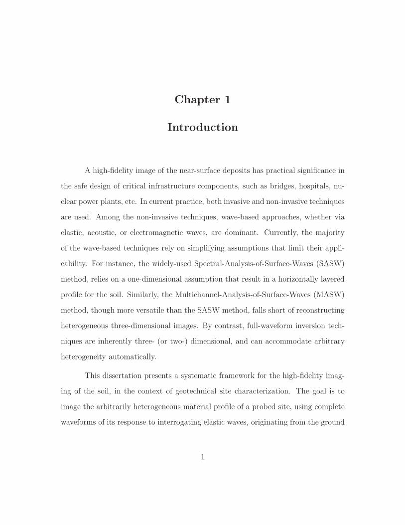
A high-fidelity image of the near-surface deposits has practical significance in
the safe design of critical infrastructure components, such as bridges, hospitals, nu-
clear power plants, etc. In current practice, both invasive and non-invasive techniques
are used. Among the non-invasive techniques, wave-based approaches, whether via
elastic, acoustic, or electromagnetic waves, are dominant. Currently, the majority
of the wave-based techniques rely on simplifying assumptions that limit their appli-
cability. For instance, the widely-used Spectral-Analysis-of-Surface-Waves (SASW)
method, relies on a one-dimensional assumption that result in a horizontally layered
profile for the soil. Similarly, the Multichannel-Analysis-of-Surface-Waves (MASW)
method, though more versatile than the SASW method, falls short of reconstructing
heterogeneous three-dimensional images. By contrast, full-waveform inversion tech-
niques are inherently three- (or two-) dimensional, and can accommodate arbitrary
heterogeneity automatically.
This dissertation presents a systematic framework for the high-fidelity imag-
ing of the soil, in the context of geotechnical site characterization. The goal is to
image the arbitrarily heterogeneous material profile of a probed site, using complete
waveforms of its response to interrogating elastic waves, originating from the ground
1
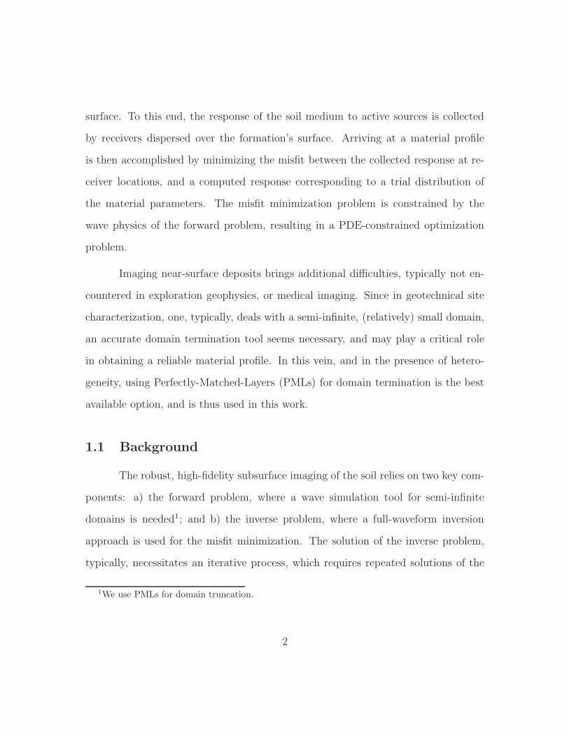
surface. To this end, the response of the soil medium to active sources is collected
by receivers dispersed over the formation’s surface. Arriving at a material profile
is then accomplished by minimizing the misfit between the collected response at re-
ceiver locations, and a computed response corresponding to a trial distribution of
the material parameters. The misfit minimization problem is constrained by the
wave physics of the forward problem, resulting in a PDE-constrained optimization
problem.
Imaging near-surface deposits brings additional difficulties, typically not en-
countered in exploration geophysics, or medical imaging. Since in geotechnical site
characterization, one, typically, deals with a semi-infinite, (relatively) small domain,
an accurate domain termination tool seems necessary, and may play a critical role
in obtaining a reliable material profile. In this vein, and in the presence of hetero-
geneity, using Perfectly-Matched-Layers (PMLs) for domain termination is the best
available option, and is thus used in this work.
1.1 Background
The robust, high-fidelity subsurface imaging of the soil relies on two key com-
ponents: a) the forward problem, where a wave simulation tool for semi-infinite
domains is needed1; and b) the inverse problem, where a full-waveform inversion
approach is used for the misfit minimization. The solution of the inverse problem,
typically, necessitates an iterative process, which requires repeated solutions of the
1We use PMLs for domain truncation.
2
forward problem, thereby accentuating the importance of an efficient and accurate
forward simulator. We review next key developments in both the forward and inverse
problems, in order to place the present work in context.
1.1.1 The perfectly-matched-layer (PML)
Numerical simulation of elastic waves in unbounded heterogeneous media has
important applications in various fields, such as seismology [1], soil-structure inter-
action [2, 3], seismic imaging [4], wave-based enhanced oil recovery [5–7], and site
characterization [8]. To keep the computation feasible, one needs to limit the extent
of the computational domain. This entails considering appropriate conditions at the
truncation boundaries such that, under ideal conditions, the boundaries become in-
visible to the outgoing waves. Perfectly-matched-layers (PML) appear to be among
the best choices for domain truncation owing, especially, to their ability to handle
heterogeneity. From a practical standpoint, implementing PML in existing codes is
also easier than competitive alternatives [9, 10]. The PML is a buffer zone that en-
forces attenuation of propagating and evanescent waves. The PML’s properties vary
gradually, from a perfectly matched interface, through a progressively attenuative
medium, to, usually, a fixed termination at the buffer zone’s end2.
The PML was first introduced by Berenger for electromagnetic waves [13].
Later, it was interpreted as a mapping of the physical coordinates onto the complex
space, referred to as complex coordinate stretching [14–16]. The interpretation al-
2Other termination conditions are also possible, including local non-reflecting boundary condi-tions [11, 12].
3
lowed the further development and adoption of the PML in elastodynamics [17, 18],
for the linearized Euler equations [19], for Helmholtz equations [9], in poroelasticity
[20], and elsewhere.
Berenger’s original development, and many other early formulations, were
based on field-splitting, which partitions a physical variable into components parallel
and perpendicular to the truncation boundary; this technique alters the structure of
the underlying differential equations and results in a manyfold increase of the number
of unknowns. Gedney [21] proposed an unsplit formulation for electromagnetic waves,
citing preservation of the Maxwellian structure, and computational efficiency among
the main advantages. Abarbanel and Gottlieb showed that Berenger’s split-form is
only weakly well-posed3, and therefore is prone to instability [23]. This motivated the
development of strongly well-posed unsplit formulations [24]; however, it turned out
that the dynamical system associated with the unsplit form suffers from degeneracy
at quiescent state, which renders the scheme unstable, and further manipulation of
the equations is necessary to ensure stability [25].
In elastodynamics, Duru and Kreiss [26] proposed a well-posed discretely-
stable unsplit formulation, and mentioned that the first-order split-form is only
weakly hyperbolic4 [27]. Among other unsplit formulations, we refer to [28–30] where
the authors’ motivation stemmed primarily from exploring alternative forms, rather
than address stability. All these developments used finite differences for spatial dis-
cretization, and exploited explicit time-stepping. Among unsplit-field finite element
3See [22] for definition of well-posedness, and hyperbolicity.4Strong hyperbolicity is a desirable property and guarantees well-posedness.
4
developments, Basu and Chopra [2] presented an, almost, displacement-only proce-
dure that relies on stress-histories and needs the evaluation of an internal force vector
at every time step, as is typically done in plasticity, via an implicit time-marching
scheme based on unsymmetric matrices. Later, Basu [31] extended this work to three-
dimensional problems, using mass-lumping and explicit time-stepping. Martin et al.
[32] developed a computationally efficient procedure that couples a velocity-stress
convolutional PML (CPML) in an ad hoc manner with a displacement-only formu-
lation in the interior domain for two-dimensional problems. The CPML formulation
was used to circumvent instabilities observed when waves travel along the inter-
face between the PML and the interior domain, when the standard PML stretching
function is used. Recently, Kucukcoban and Kallivokas [33] developed a symmet-
ric displacement-stress formulation, using mixed-field finite elements for the PML,
coupled with standard displacement-only finite elements for the interior domain, us-
ing the standard Newmark method for time integration. We remark that implicit
time-stepping can become challenging for large-scale three-dimensional problems and
should be avoided if possible.
The literature on split-field elastodynamics is rich. This approach is particu-
larly attractive because, normally, it does not use convolutions or auxiliary variables.
However, it almost always results in using mixed schemes, i.e., treating velocity and
stress components (or a similar combination) as unknowns over the entire domain.
Table 1.1 summarizes key developments in time-domain elastodynamics based on four
categories: split- or unsplit-field formulation, and finite difference or finite/spectral
element implementation.
5
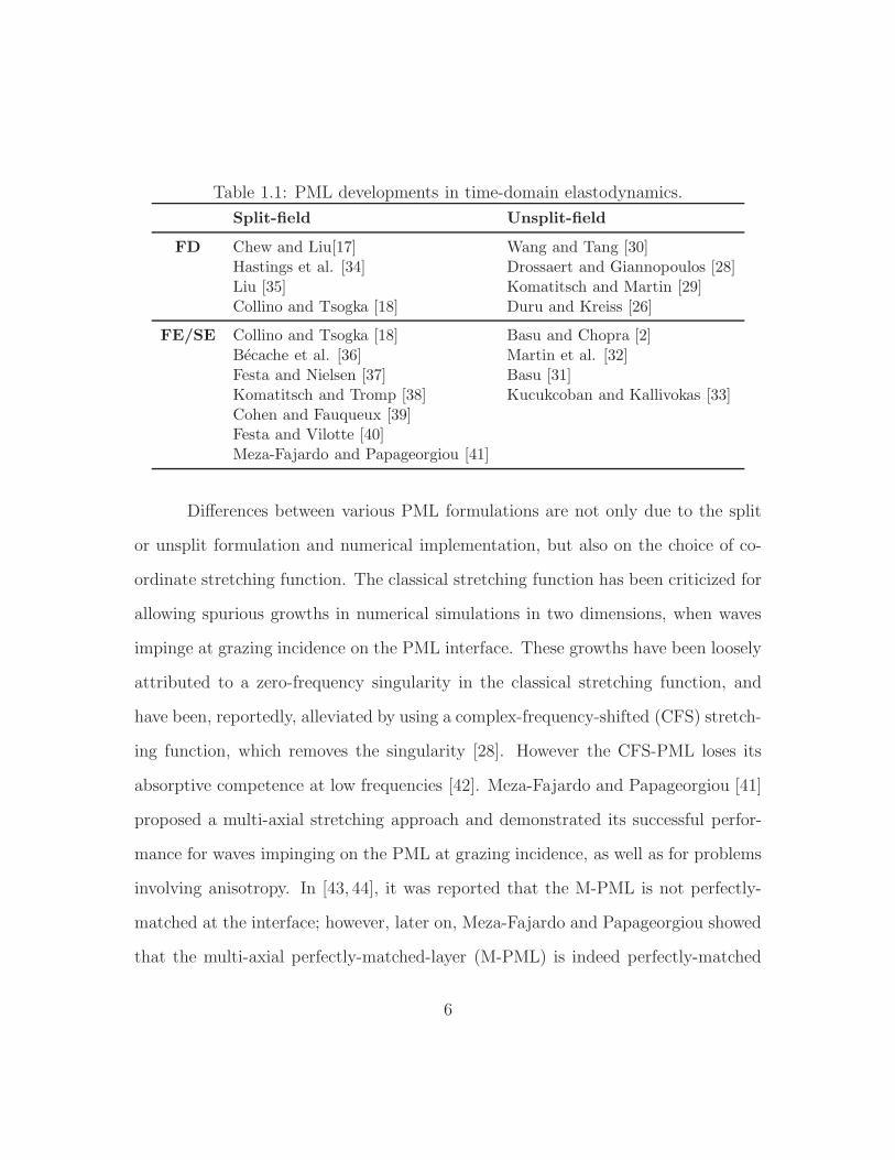
Table 1.1: PML developments in time-domain elastodynamics.
Split-field Unsplit-field
FD Chew and Liu[17] Wang and Tang [30]Hastings et al. [34] Drossaert and Giannopoulos [28]Liu [35] Komatitsch and Martin [29]Collino and Tsogka [18] Duru and Kreiss [26]
FE/SE Collino and Tsogka [18] Basu and Chopra [2]Becache et al. [36] Martin et al. [32]Festa and Nielsen [37] Basu [31]Komatitsch and Tromp [38] Kucukcoban and Kallivokas [33]Cohen and Fauqueux [39]Festa and Vilotte [40]Meza-Fajardo and Papageorgiou [41]
Differences between various PML formulations are not only due to the split
or unsplit formulation and numerical implementation, but also on the choice of co-
ordinate stretching function. The classical stretching function has been criticized for
allowing spurious growths in numerical simulations in two dimensions, when waves
impinge at grazing incidence on the PML interface. These growths have been loosely
attributed to a zero-frequency singularity in the classical stretching function, and
have been, reportedly, alleviated by using a complex-frequency-shifted (CFS) stretch-
ing function, which removes the singularity [28]. However the CFS-PML loses its
absorptive competence at low frequencies [42]. Meza-Fajardo and Papageorgiou [41]
proposed a multi-axial stretching approach and demonstrated its successful perfor-
mance for waves impinging on the PML at grazing incidence, as well as for problems
involving anisotropy. In [43, 44], it was reported that the M-PML is not perfectly-
matched at the interface; however, later on, Meza-Fajardo and Papageorgiou showed
that the multi-axial perfectly-matched-layer (M-PML) is indeed perfectly-matched
6
in Berenger’s sense, and it provides domain truncations that are at least as accu-
rate as the classical PML, when the latter is stable [45]. In a more recent study,
Ping et al. [46] have shown results according to which M-PML may perform less
accurately than the classical PML. Our own experience, both in two-dimensional
and three-dimensional simulations, is also more in accordance with Ping et al. [46].
It also seems that the original M-PML development is mathematically inconsistent
due to the improper definition of the Jacobian of the transformation. We discuss
this issue in Section 2.6. Herein, we opt for classical stretching functions for their
simplicity, satisfactory performance when parametrized carefully, and their accuracy
in low frequencies, which is important in site characterization problems [8]. We also
discuss how our formulation can accommodate the multi-axial stretching through
simple modifications.
1.1.2 Full-waveform inversion (FWI)
Seismic inversion refers to the process of identification of material properties in
geological formations [47–49]. The problem arises predominantly in exploration geo-
physics [50–53] and geotechnical site characterization [8]; it belongs to the broader
class of inverse medium problems: waves, whether of acoustic, elastic, or electro-
magnetic nature, are used to interrogate a medium, and the medium’s response
to the probing is subsequently used to image the spatial distribution of properties
(e.g., Lame parameters, or wave velocities) [54–56]. Mathematically, algorithmically,
and computationally, inverse medium problems are challenging, especially, when no
a priori constraining assumption is made on the spatial variability of the medium’s
7
properties. The challenges are further compounded when the underlying physics is
time-dependent, and involves more than a single distributed parameter to be inverted
for, as in seismic inversion.
Due to the complexity of the inverse problem at hand, most techniques to date
rely on simplifying assumptions, aiming at rendering a solution to the problem more
tractable. These assumptions can be divided into four categories: a) assumptions
regarding the dimensionality of the problem, whereby the original problem is reduced
to a two-dimensional [8, 57], or a one-dimensional problem [58]; b) assuming that the
dominant portion of the wave energy on the ground surface is transported through
Rayleigh waves, and thus, disregarding other wave types, such as compressional
and shear waves, as is the case in the Spectral-Analysis-of-Surface-Waves (SASW)
and its variants (MASW) [59]; c) inverting for only one parameter, as is done in
[60–63], where inversion was attempted only for the shear wave velocity, assuming
the compressional wave velocity (or an equivalent counterpart) is known; and d)
assumptions concerning the truncation boundaries, which are oftentimes, grossly
simplified due to the complexity associated with the rigorous treatment of these
boundaries [64]. Over the past decade, continued advances in both algorithms and
computer architectures have allowed the gradual removal of the limitations of existing
methodologies. However, a robust methodology, especially for the time-dependent
elastic case remains, by and large, elusive.
Among the recent works on inversion, which are similar in character to ours,
we refer to Pratt et al. [65] who considered two-dimensional acoustic inversion in
the frequency domain, and Epanomeritakis et al. [61] where full-waveform inversion
8
has attempted for three-dimensional time-domain elastodynamics, where a simple
boundary condition was used for domain truncation. Kang and Kallivokas [56] con-
sidered the problem for the two-dimensional time-domain acoustic case, and used
PMLs to accurately account for domain truncation. Kucukcoban [57] extended the
work of Kang and Kallivokas to two-dimensional elastodynamics, and reported suc-
cessful reconstruction of the two Lame parameters for models involving synthetic
data. Recently, Bramwell [66] used a discontinuous Petrov-Galerkin (DPG) method
in the frequency domain, endowed with PMLs, for seismic tomography problems,
advocating the DPG scheme over conventional continuous Galerkin methods, since
it results in less numerical pollution.
This dissertation extends the work of Kucukcoban [57] to three-dimensional
elastodynamics. We remark that PMLs add significant complexity to the solution
of both the forward and the inverse problem. Moreover, since we target three-
dimensional problems, using scalable parallel algorithms is essential.
1.2 Present approach
In this dissertation, we discuss a systematic framework for the numerical res-
olution of the inverse medium problem, directly in the time-domain, in the context
of geotechnical site characterization. As discussed in the introduction, the goal is to
image the arbitrarily heterogeneous material profile of a probed soil medium, using
complete waveforms5 of its response to interrogating elastic waves, originating from
5Using the complete waveform (complete recorded response) results in a full-waveform inversionapproach.
9
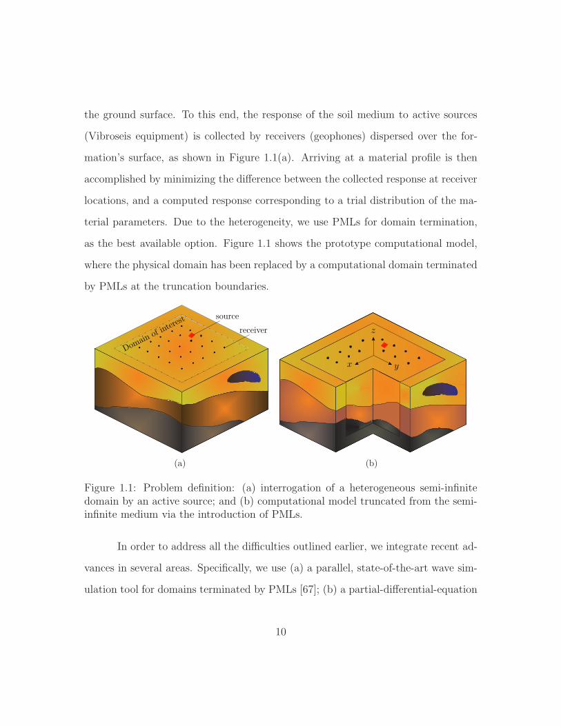
the ground surface. To this end, the response of the soil medium to active sources
(Vibroseis equipment) is collected by receivers (geophones) dispersed over the for-
mation’s surface, as shown in Figure 1.1(a). Arriving at a material profile is then
accomplished by minimizing the difference between the collected response at receiver
locations, and a computed response corresponding to a trial distribution of the ma-
terial parameters. Due to the heterogeneity, we use PMLs for domain termination,
as the best available option. Figure 1.1 shows the prototype computational model,
where the physical domain has been replaced by a computational domain terminated
by PMLs at the truncation boundaries.
(a)
x y
z
(b)
Figure 1.1: Problem definition: (a) interrogation of a heterogeneous semi-infinitedomain by an active source; and (b) computational model truncated from the semi-infinite medium via the introduction of PMLs.
In order to address all the difficulties outlined earlier, we integrate recent ad-
vances in several areas. Specifically, we use (a) a parallel, state-of-the-art wave sim-
ulation tool for domains terminated by PMLs [67]; (b) a partial-differential-equation
10
(PDE)-constrained optimization framework through which the minimization of the
difference between the collected response at receiver locations and a computed re-
sponse corresponding to a trial distribution of the material properties is attained [68];
(c) regularization schemes to alleviate the ill-posedness inherent in inverse problems;
(d) continuation schemes that lend algorithmic robustness [56]; and (e) a biasing
scheme that accelerates the convergence of the λ-profile for robust simultaneous in-
version of both Lame parameters [57].
1.3 Contributions
This work builds and improves upon the Ph.D. dissertation of Sezgin Kucuk-
coban in two-dimensional elastic full-waveform inversion [57]. Key contributions of
the present development are listed below.
In three dimensions:
• Developing a new PML formulation for the simulation of elastic waves in three-
dimensional, arbitrarily heterogeneous, semi-infinite media, where a stress-
displacement formulation for the PML, is coupled with a standard displacement-
only formulation for the interior domain. This hybrid treatment leads to a
computationally cost-efficient scheme. The formulation builds and improves
upon a recently developed two-dimensional scheme [33]. However, it is restruc-
tured, and modified, to accommodate explicit time-stepping, which makes it
suitable for large-scale problems on parallel computers [67].
• Presenting a robust full-waveform inversion methodology for three-dimensional,
11

arbitrarily heterogeneous, PML-truncated, elastic formations, leading to the
successful reconstruction of the spatially-distributed Lame parameters. A con-
sistent finite element approach was used throughout. The accuracy of the
discrete gradients, computed from this scheme, are verified by comparing them
with directional finite differences [69]. The developed framework was used
for the three-dimensional characterization of the NEES@UCSB site in Garner
Valley, CA [70].
In two dimensions:
• Developing a discretize-then-optimize scheme for the accurate computation of
the discrete gradients of the discrete objective functional. Accordingly, the
objective functional is discretized first, followed by differentiation, to yield
discrete gradients, which can then be used in a gradient-based optimization
scheme [8].
• Developing a practical procedure to accommodate field data, which are inher-
ently three-dimensional, into two-dimensional full-waveform-inversion-based co-
des. Designing and conducting a field experiment at the Hornsby Bend site in
Austin, TX, whose records were subsequently used to drive the inversion al-
gorithms in order to characterize the site where the experiment took place
[8].
1.4 Dissertation outline
The rest of this dissertation is organized as follows:
12
Chapter 2 presents a new PML formulation for the simulation of elastic waves
in three-dimensional, arbitrarily heterogeneous domains. We begin with reviewing
key ideas for developing a PML, and discuss complex coordinate stretching. Then, we
present a stress-displacement formulation for the PML, which leads to a third-order-
in-time semi-discrete form. We discuss how this formulation can be coupled with
a standard displacement-only formulation for the interior domain, thus leading to
a computationally cost-efficient scheme. We discuss several time-marching schemes.
In particular, we discuss an explicit, fourth-order, Runge-Kutta scheme which is
well-suited for large-scale problems on parallel computers. In Section 2.5, we discuss
an alternative formulation for the PML that leads to a symmetric semi-discrete
form. In Section 2.6 we show how our formulation can accommodate multi-axial
PML (M-PML), by simple modifications. Lastly, we provide numerical experiments
demonstrating stability and efficacy of the proposed formulations.
In Chapter 3, we consider the inverse medium problem in three-dimensional,
PML-truncated domains, using full-waveforms. We cast the associated inverse prob-
lem, as a misfit minimization problem, using the apparatus of PDE-constrained opti-
mization to impose the forward wave propagation equations, followed by computing
the optimality system. Next, we discuss strategies that alleviate ill-posedness, and
lend algorithmic robustness to our proposed inversion scheme. By using a numerical
experiment, we verify the accuracy of the gradients computed via the control prob-
lems, by comparing them with directional finite differences. We present numerical
experiments demonstrating successful reconstruction of the two Lame parameters for
smooth and sharp profiles, using noise-free and also highly-noisy synthetic data.
13

In Chapter 4, we discuss a full-waveform inversion methodology for site char-
acterization, using field data. We start by reviewing the two-dimensional forward
wave propagation in PML-truncated domains, followed by presenting a robust ap-
proach to tackle the associated inverse medium problem. We then report on the
design and data processing of a field experiment, whose records were used along
with the presented two-dimensional framework, to obtain the compressional, and
shear wave velocity profile of the site where the experiment took place. Next, we
compare the profiles with those obtained from the SASW method, and invasive Cone
Penetrometer Tests (CPTs). Lastly, we use the methodology described in Chapter
3 for the three-dimensional site characterization of the NEES site in Garner Valley,
CA.
We conclude with summary remarks in Chapter 5, and suggest future direc-
tions.
14
Chapter 2
Simulation of wave motion in three-dimensional
PML-truncated heterogeneous media
In this chapter, we discuss the development and parallel implementation of an
unsplit-field, displacement-stress PML formulation, using mixed-field finite elements
for the PML, which when coupled with a standard displacement-only finite element
formulation for the interior domain, leads to the efficient simulation of wave motion
in physically unbounded, three-dimensional, arbitrarily heterogeneous elastic media.
The hybrid treatment of coupling a mixed-field PML with a single-field interior-
domain leads to optimal computational cost and allows for ready incorporation of
the PML in existing closed-domain standard finite element codes, by simply attaching
the matrices corresponding to the PML buffer. The resulting semi-discrete form is
unsymmetric and third-order in time. Using spectral elements, we render the mass
matrix diagonal and exploit explicit time-stepping via the Runge-Kutta method. We
also present an alternative formulation, which results in a fully symmetric discrete
form, at the expense of utilizing an implicit time-marching scheme. We discuss how
the standard Newmark scheme can also be used for time integration. This work builds
and improves upon recent developments [33, 71] in two-dimensional elastodynamics.
15

2.1 Complex-coordinate-stretching
In this section, we briefly review the key features of the PML. Part of the
material discussed here is not new; however, it is provided to allow for context and
completeness.
2.1.1 Key idea
The key idea in constructing a PML is based on analytic continuation of so-
lutions of wave equations. This amounts to mapping the spatial coordinates onto
the complex space, using the, so-called, stretching functions. For instance, one-
dimensional outgoing waves propagate according to uout(x, t) = e−ik(x−ct), where
k is the wavenumber, and c denotes wave speed. After applying the mapping1
x 7→ ζ(x) + 1iω
η(x), we obtain uoutPML(x, t) = e−ik(ζ(x)−ct)e−η(x)/c, where the lat-
ter term enforces spatial attenuation. A similar argument also holds for evanescent
waves.
In practice, the PML has a limited thickness (see Fig. 2.1), and is termi-
nated with a fixed boundary. Therefore, reflections (i.e., incoming waves) could
develop when outgoing waves hit the fixed boundary of the PML layer. In our
one-dimensional example, uincPML(x, t) = eik(ζ(x)+ct)eη(x)/c. Since η(x) is a positive,
monotonically increasing function of x, reflected waves also get attenuated, due to
decreasing x. Hence, the PML attenuates both outgoing and incoming waves.
We briefly discuss the principal components required for constructing a PML.
1ζ(x), η(x) are positive, monotonically increasing functions of x.
16
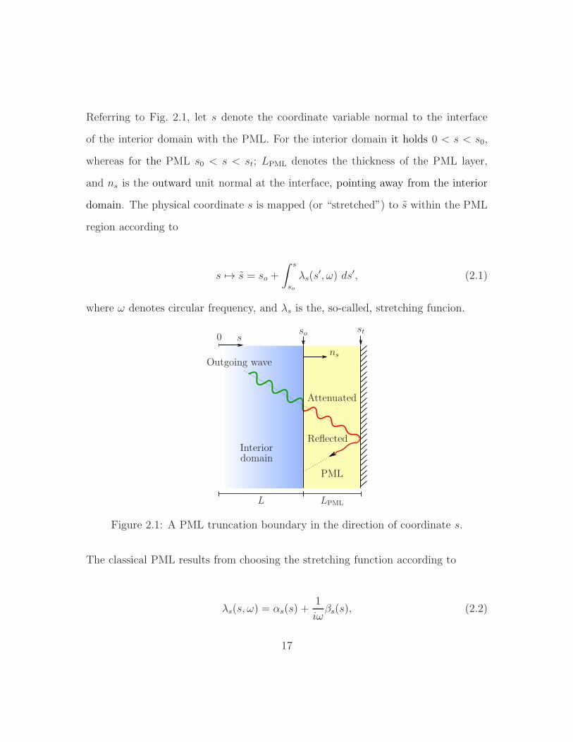
Referring to Fig. 2.1, let s denote the coordinate variable normal to the interface
of the interior domain with the PML. For the interior domain it holds 0 < s < s0,
whereas for the PML s0 < s < st; LPML denotes the thickness of the PML layer,
and ns is the outward unit normal at the interface, pointing away from the interior
domain. The physical coordinate s is mapped (or “stretched”) to s within the PML
region according to
s 7→ s = so +
∫ s
so
λs(s′, ω) ds′, (2.1)
where ω denotes circular frequency, and λs is the, so-called, stretching funcion.
Interiordomain
PML
Outgoing wave
Attenuated
Reflected
LPMLL
s
ns
sost
0
Figure 2.1: A PML truncation boundary in the direction of coordinate s.
The classical PML results from choosing the stretching function according to
λs(s, ω) = αs(s) +1
iωβs(s), (2.2)
17
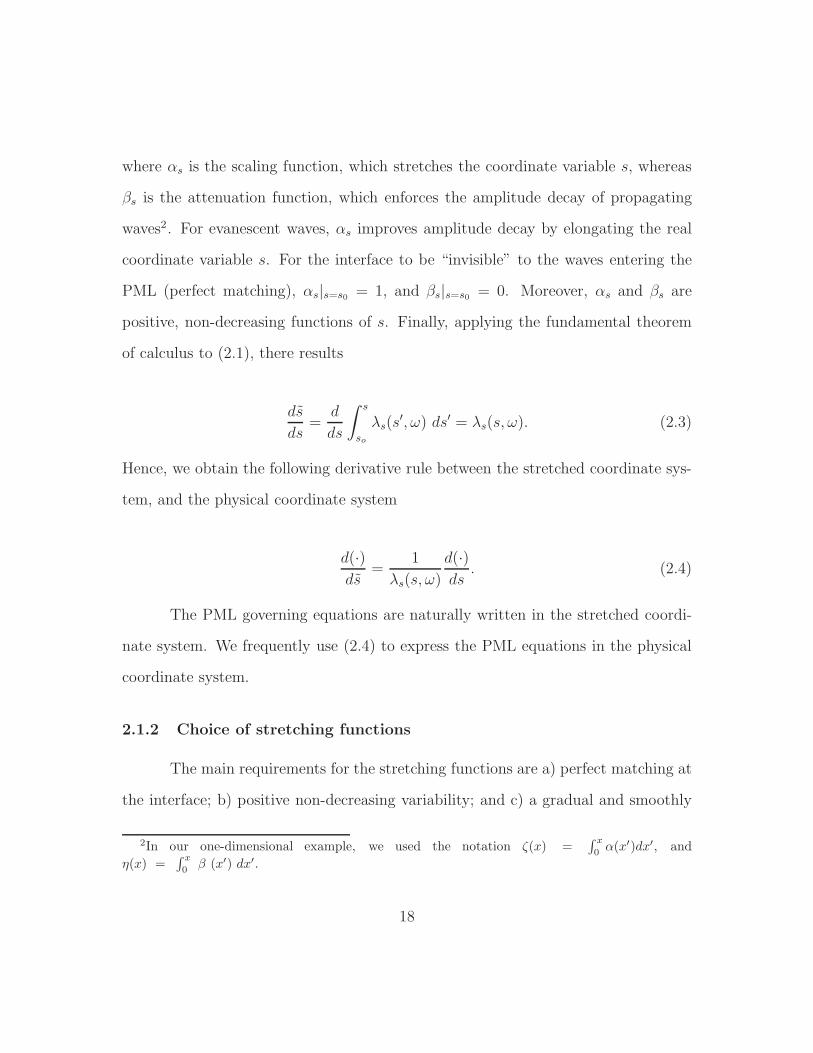
where αs is the scaling function, which stretches the coordinate variable s, whereas
βs is the attenuation function, which enforces the amplitude decay of propagating
waves2. For evanescent waves, αs improves amplitude decay by elongating the real
coordinate variable s. For the interface to be “invisible” to the waves entering the
PML (perfect matching), αs|s=s0 = 1, and βs|s=s0 = 0. Moreover, αs and βs are
positive, non-decreasing functions of s. Finally, applying the fundamental theorem
of calculus to (2.1), there results
ds
ds=
d
ds
∫ s
so
λs(s′, ω) ds′ = λs(s, ω). (2.3)
Hence, we obtain the following derivative rule between the stretched coordinate sys-
tem, and the physical coordinate system
d(·)ds
=1
λs(s, ω)
d(·)ds
. (2.4)
The PML governing equations are naturally written in the stretched coordi-
nate system. We frequently use (2.4) to express the PML equations in the physical
coordinate system.
2.1.2 Choice of stretching functions
The main requirements for the stretching functions are a) perfect matching at
the interface; b) positive non-decreasing variability; and c) a gradual and smoothly
2In our one-dimensional example, we used the notation ζ(x) =∫ x
0α(x′)dx′, and
η(x) =∫ x
0β (x′) dx′.
18
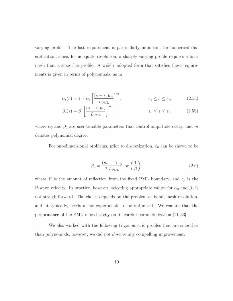
varying profile. The last requirement is particularly important for numerical dis-
cretization, since, for adequate resolution, a sharply varying profile requires a finer
mesh than a smoother profile. A widely adopted form that satisfies these require-
ments is given in terms of polynomials, as in
αs(s) = 1 + αo
[(s− so)ns
LPML
]m, so ≤ s ≤ st, (2.5a)
βs(s) = βo
[(s− so)ns
LPML
]m, so ≤ s ≤ st, (2.5b)
where α0 and β0 are user-tunable parameters that control amplitude decay, and m
denotes polynomial degree.
For one-dimensional problems, prior to discretization, β0 can be shown to be
β0 =(m+ 1) cp2 LPML
log
(1
R
), (2.6)
where R is the amount of reflection from the fixed PML boundary, and cp is the
P-wave velocity. In practice, however, selecting appropriate values for α0 and β0 is
not straightforward. The choice depends on the problem at hand, mesh resolution,
and, it typically, needs a few experiments to be optimized. We remark that the
performance of the PML relies heavily on its careful parameterization [11, 33].
We also worked with the following trigonometric profiles that are smoother
than polynomials; however, we did not observe any compelling improvement.
19
αs(s) = 1 +αo
2
[1 + sin
(π( |s− so|
LPML− 1
2
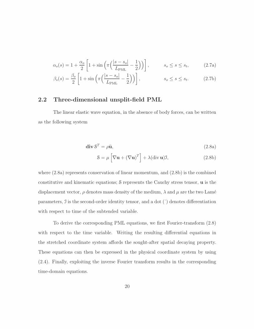
))], so ≤ s ≤ st, (2.7a)
βs(s) =βo
2
[1 + sin
(π( |s− so|
LPML
− 1
2
))], so ≤ s ≤ st. (2.7b)
2.2 Three-dimensional unsplit-field PML
The linear elastic wave equation, in the absence of body forces, can be written
as the following system
div ST = ρu, (2.8a)
S = µ[∇u+ (∇u)T
]+ λ(divu)I, (2.8b)
where (2.8a) represents conservation of linear momentum, and (2.8b) is the combined
constitutive and kinematic equations; S represents the Cauchy stress tensor, u is the
displacement vector, ρ denotes mass density of the medium, λ and µ are the two Lame
parameters, I is the second-order identity tensor, and a dot (˙) denotes differentiation
with respect to time of the subtended variable.
To derive the corresponding PML equations, we first Fourier-transform (2.8)
with respect to the time variable. Writing the resulting differential equations in
the stretched coordinate system affords the sought-after spatial decaying property.
These equations can then be expressed in the physical coordinate system by using
(2.4). Finally, exploiting the inverse Fourier transform results in the corresponding
time-domain equations.
20
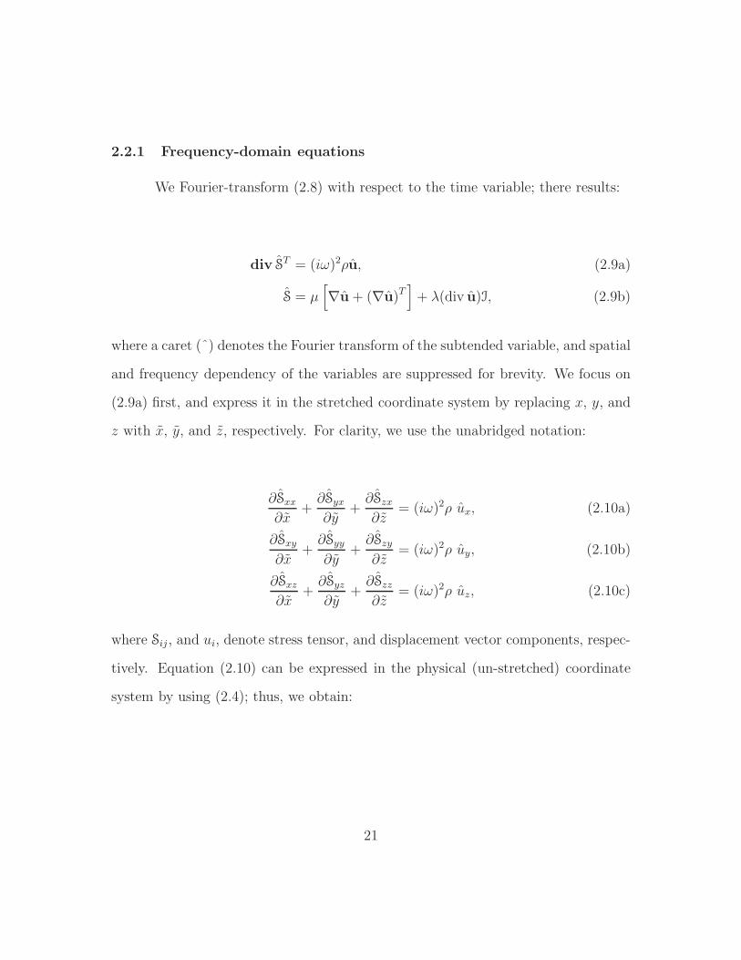
2.2.1 Frequency-domain equations
We Fourier-transform (2.8) with respect to the time variable; there results:
div ST = (iω)2ρu, (2.9a)
S = µ[∇u+ (∇u)T
]+ λ(div u)I, (2.9b)
where a caret (ˆ) denotes the Fourier transform of the subtended variable, and spatial
and frequency dependency of the variables are suppressed for brevity. We focus on
(2.9a) first, and express it in the stretched coordinate system by replacing x, y, and
z with x, y, and z, respectively. For clarity, we use the unabridged notation:
∂Sxx
∂x+
∂Syx
∂y+
∂Szx
∂z= (iω)2ρ ux, (2.10a)
∂Sxy
∂x+
∂Syy
∂y+
∂Szy
∂z= (iω)2ρ uy, (2.10b)
∂Sxz
∂x+
∂Syz
∂y+
∂Szz
∂z= (iω)2ρ uz, (2.10c)
where Sij , and ui, denote stress tensor, and displacement vector components, respec-
tively. Equation (2.10) can be expressed in the physical (un-stretched) coordinate
system by using (2.4); thus, we obtain:
21
1
λx
∂Sxx
∂x+
1
λy
∂Syx
∂y+
1
λz
∂Szx
∂z= (iω)2ρ ux, (2.11a)
1
λx
∂Sxy
∂x+
1
λy
∂Syy
∂y+
1
λz
∂Szy
∂z= (iω)2ρ uy, (2.11b)
1
λx
∂Sxz
∂x+
1
λy
∂Syz
∂y+
1
λz
∂Szz
∂z= (iω)2ρ uz. (2.11c)
Multiplying (2.11) through by λxλyλz results in
div(STΛ
)= (iω)2ρ λxλyλz u, (2.12)
where the stretching tensor Λ is defined as
Λ =
λyλz 0 00 λxλz 00 0 λxλy
=
αyαz 0 00 αxαz 00 0 αxαy
+1
(iω)
αyβz + αzβy 0 0
0 αxβz + αzβx 00 0 αxβy + αyβx
+1
(iω)2
βyβz 0 00 βxβz 00 0 βxβy
= Λe +
1
iωΛp +
1
(iω)2Λw. (2.13)
We remark that within the interior domain, Λe reduces to the identity ten-
sor, whereas Λp and Λw vanish identically. Substituting (2.13) and (2.2) in (2.12),
rearranging and grouping similar terms, results in
div
(STΛe +
1
iωSTΛp +
1
(iω)2STΛw
)= ρ
[(iω)2au+ iωbu+ cu+
d
iωu
], (2.14)
22
where
a = αx αy αz,
b = αx αy βz + αx αz βy + αy αz βx,
c = αx βy βz + αy βz βx + αz βy βx,
d = βx βy βz. (2.15)
Multiplying (2.14) by iω, we obtain
div
(iωSTΛe + STΛp +
1
iωSTΛw
)= ρ
[(iω)3au+ (iω)2bu+ iωcu+ du
]. (2.16)
Next, we focus our attention on the combined constitutive and kinematic
equations (2.9b). Writing (2.9b) in the stretched coordinate system, and using (2.4)
to express it in the physical coordinate system, there results
S = µ
(∇u)
1λx
0 0
0 1λy
0
0 0 1λz
+
1λx
0 0
0 1λy
0
0 0 1λz
(∇u)T
+ λ( 1
λx
∂ux
∂x+
1
λy
∂uy
∂y+
1
λz
∂uz
∂z
)I. (2.17)
Multiplying (2.17) by λxλyλz results in
λxλyλzS = µ[∇u Λ + Λ (∇u)T
]+ λ div(Λu)I, (2.18)
where the stretching tensor Λ is defined in (2.13). Multiplying (2.18) by (iω)2 and
using (2.13), and (2.2), rearranging and grouping similar terms, we obtain
23
(iω)2aS+ iωbS + cS+1
iωdS = µ(iω)2
[(∇u)Λe + Λe(∇u)T
]
+ µ iω[(∇u)Λp + Λp(∇u)T
]+ µ
[(∇u)Λw + Λw(∇u)T
]
+ λ(iω)2 div(Λeu)I+ λ iω div(Λpu)I+ λ div(Λwu)I. (2.19)
Equations (2.16) and (2.19) constitute the corresponding frequency-domain momen-
tum, and combined constitutive and kinematic equations in the stretched coordinate
system, respectively. They possess the desired spatial decaying property.
2.2.2 Time-domain equations
In this section, we apply the inverse Fourier transform to (2.16) and (2.19)
to obtain the corresponding time-domain equations. This operation is rather simple
due to the specific choice of the stretching function (2.2). We use
F−1
[g(ω)
iω
]=
∫ t
0
g(τ)dτ, (2.20)
where F−1 denotes the inverse Fourier transform operator3, and g(t) is a sufficiently
regular function. Applying the inverse Fourier transform to (2.16) and (2.19), we
obtain
3In general, F−1[g(ω)iω
]=
∫ t
0 g(τ)dτ−πg(0)δ(ω), but, it can be shown that since, by construction,
the overall development excludes ω = 0, the inverse transform reduces to (2.20) [71].
24
div
[STΛe + STΛp +
(∫ t
0
STdτ
)Λw
]= ρ (a
...u+ bu+ cu+ du) , (2.21a)
aS+ bS + cS+ d
(∫ t
0
Sdτ
)=
µ[(∇u)Λe + Λe(∇u)T + (∇u)Λp + Λp(∇u)T + (∇u)Λw + Λw(∇u)T
]+
λ [div(Λeu) + div(Λpu) + div(Λwu)] I. (2.21b)
The set of integro-differential equations (2.21) can be expressed as a set of
only partial differential equations, upon introducing the auxiliary variable S(x, t),
which may be interpreted as the stress history tensor [71, 72]:
S(x, t) =
∫ t
0
S(x, τ)dτ. (2.22a)
Clearly,
S(x, t) = S(x, t), S(x, t) = S(x, t),...S(x, t) = S(x, t). (2.22b)
Substituting (2.22) in (2.21), we obtain
div(STΛe + STΛp + STΛw
)= ρ (a
...u+ bu+ cu+ du) , (2.23a)
a...S+ bS+ cS+ dS =
µ[(∇u)Λe + Λe(∇u)T + (∇u)Λp + Λp(∇u)T + (∇u)Λw + Λw(∇u)T
]+
λ [div(Λeu) + div(Λpu) + div(Λwu)] I. (2.23b)
25
Equations (2.23) constitute the corresponding time-domain PML momentum,
and combined constitutive and kinematic equations.
2.3 Hybrid finite element implementation
In this section, we discuss an efficient finite element technique for transient
elastodynamics in PML-truncated domains. We use a method-of-lines approach,
where we exploit a Galerkin method for spatial discretization, thus, obtaining a
third-order, continuous-in-time system of ordinary differential equations. Various
methods exist for time-integration of such systems. We discuss three techniques that
seem suitable for practical applications.
2.3.1 Spatial discretization
The PML equations (2.23) can be used both for the interior domain and the
PML buffer zone, since by construction, they reduce to (2.8) in the interior domain.
This unified treatment amounts to considering stress and displacement components
as unknowns in both the interior domain and the PML buffer zone. While feasible
in principle, as is done in most PML formulations to date, we opt for a hybrid treat-
ment, originally developed in [33] for two-dimensional problems, where the interior
domain is treated with a standard displacement-only formulation, coupled with the
PML equations in the buffer zone. This approach results in substantial reduction
in computational cost compared to mixed-field formulations cast over the entire do-
main. It also makes the modification of existing interior-domain elastodynamic codes
straightforward, since, one needs to only add the PML-related forms, whereas for the
26
most part, the general structure of such codes remains intact.
Accordingly, find u(x, t) in ΩRD ∪ΩPML, and S(x, t) in ΩPML (see Fig. 2.2 for
domain and boundary designations), where u and S reside in appropriate function
spaces, and:
divµ[∇u+ (∇u)T
]+ λ(div u)I
+ b = ρ
...u in ΩRD × J,
(2.24a)
div(STΛe + STΛp + STΛw
)= ρ (a
...u+ bu+ cu+ du) in ΩPML × J,
(2.24b)
a...S+ bS+ cS+ dS =
µ[(∇u)Λe + Λe(∇u)T + (∇u)Λp + Λp(∇u)T + (∇u)Λw + Λw(∇u)T
]+
λ [div(Λeu) + div(Λpu) + div(Λwu)] I in ΩPML × J.(2.24c)
The system is initially at rest, and subject to the following boundary and interface
conditions:
µ[∇u+ (∇u)T
]+ λ(div u)I
n+ = gn on ΓRD
N × J,(2.25a)
(STΛe + STΛp + STΛw)n− = 0 on ΓPML
N × J,(2.25b)
u = 0 on ΓPMLD × J,(2.25c)
u+ = u− on ΓI × J,(2.25d)
µ[∇u+ (∇u)T
]+ λ(div u)I
n+ + (STΛe + STΛp + STΛw)n
− = 0 on ΓI × J,(2.25e)
27
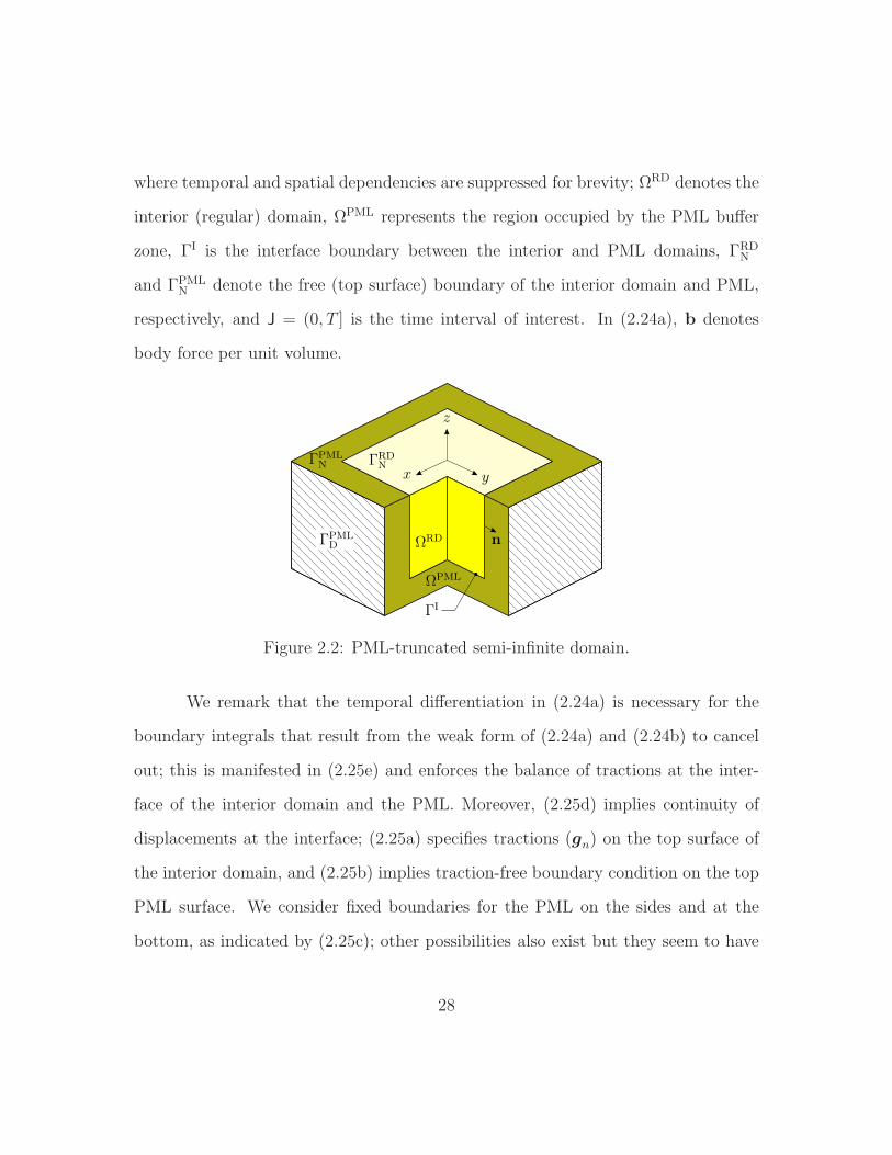
where temporal and spatial dependencies are suppressed for brevity; ΩRD denotes the
interior (regular) domain, ΩPML represents the region occupied by the PML buffer
zone, ΓI is the interface boundary between the interior and PML domains, ΓRDN
and ΓPMLN denote the free (top surface) boundary of the interior domain and PML,
respectively, and J = (0, T ] is the time interval of interest. In (2.24a), b denotes
body force per unit volume.
n
y
z
Figure 2.2: PML-truncated semi-infinite domain.
We remark that the temporal differentiation in (2.24a) is necessary for the
boundary integrals that result from the weak form of (2.24a) and (2.24b) to cancel
out; this is manifested in (2.25e) and enforces the balance of tractions at the inter-
face of the interior domain and the PML. Moreover, (2.25d) implies continuity of
displacements at the interface; (2.25a) specifies tractions (gn) on the top surface of
the interior domain, and (2.25b) implies traction-free boundary condition on the top
PML surface. We consider fixed boundaries for the PML on the sides and at the
bottom, as indicated by (2.25c); other possibilities also exist but they seem to have
28
little influence on performance [11, 12].
Next, we seek a weak solution, corresponding to the strong form of (2.24)
and (2.25), in the Galerkin sense. Specifically, we take the inner products of (2.24a)
and (2.24b) with (vector) test function w(x), and integrate by parts over their cor-
responding domains. Incorporating (2.25d-2.25e) eliminates the interface boundary
terms and results in (2.26a). Next, we take the inner product of (2.24c) with (tensor)
test function T(x); there results (2.26b). There are other possibilities for deriving a
weak form that corresponds to the strong form (2.24) and (2.25). We refer to [73]
for further details.
Accordingly, find u ∈ H1(Ω)× J, and S ∈ L2(Ω)× J, such that:
∫
ΩRD
∇w :µ[∇u+ (∇u)T
]+ λ(div u)I
dΩ +
∫
ΩPML
∇w :(STΛe + STΛp + STΛw
)dΩ
+
∫
ΩRD
w · ρ...u dΩ +
∫
ΩPML
w · ρ (a...u+ bu+ cu+ du) dΩ =
∫
ΓRD
N
w · gn dΓ +
∫
ΩRD
w · b dΩ,
(2.26a)∫
ΩPML
T :(a...S+ bS+ cS+ dS
)dΩ
=
∫
ΩPML
T :µ[(∇u)Λe + Λe(∇u)T + (∇u)Λp + Λp(∇u)T + (∇u)Λw + Λw(∇u)T
]
+T :λ [div(Λeu) + div(Λpu) + div(Λwu)] I dΩ, (2.26b)
for every w ∈ H1(Ω) and T ∈ L2(Ω), where gn ∈ L2(Ω) × J, and b ∈ L2(Ω) × J.
Function spaces for scalar- (v), vector- (v), and tensor-valued (A) functions are
defined as
29
L2(Ω) =
v :
∫
Ω
|v|2dx <∞, (2.27a)
L2(Ω) =v : v ∈ (L2(Ω))3
, (2.27b)
L2(Ω) =A : A ∈ (L2(Ω))3×3
, (2.27c)
H1(Ω) =
v :
∫
Ω
(|v|2 + |∇v|2
)dx <∞, v|ΓPML
D
= 0
, (2.27d)
H1(Ω) =v : v ∈ (H1(Ω))3
. (2.27e)
In order to resolve (2.26) numerically, we use standard finite-dimensional sub-
spaces. Specifically, we introduce finite-dimensional subspaces Ξh ⊂ H1(Ω) and
Υh ⊂ L2(Ω), with basis functions Φ and Ψ, respectively. We then approximate
u(x, t) with uh(x, t) ∈ Ξh × J, and S(x, t) with Sh(x, t) ∈ Υh × J, as detailed below
uh(x, t) =
ΦT (x)ux(t)ΦT (x)uy(t)ΦT (x)uz(t)
, (2.28a)
Sh(x, t) =
ΨT (x)Sxx(t) ΨT (x)Sxy(t) ΨT (x)Sxz(t)ΨT (x)Syx(t) ΨT (x)Syy(t) ΨT (x)Syz(t)ΨT (x)Szx(t) ΨT (x)Szy(t) ΨT (x)Szz(t)
. (2.28b)
In a similar fashion, we approximate the test functions, w(x) with wh(x) ∈
Ξh, and T(x) with Th(x) ∈ Υh; therefore:
30
wh(x) =
wT
xΦ(x)wT
y Φ(x)wT
z Φ(x)
, (2.29a)
Th(x) =
TT
xxΨ(x) TTxyΨ(x) TT
xzΨ(x)TT
yxΨ(x) TTyyΨ(x) TT
yzΨ(x)TT
zxΨ(x) TTzyΨ(x) TT
zzΨ(x)
. (2.29b)
Incorporating (2.28-2.29) into (2.26), results in the following semi-discrete form
M...d+Cd+Kd+Gd = f , (2.30)
where spatial and temporal dependencies are suppressed for brevity, and system
matrices, M, C, K, G, and vectors d and f , are defined as
M =
[MRD + Ma 0
0 Na
], C =
[Mb Aeu
−ATel Nb
], (2.31a)
K =
[KRD + Mc Apu
−ATpl Nc
], G =
[Md Awu
−ATwl Nd
], (2.31b)
d =[uh Sh
]T, f =
[fRD 0
]T, (2.31c)
where subscript RD refers to the interior (regular) domain, and MRD, KRD, and fRD,
correspond to the standard mass matrix, stiffness matrix, and vector of nodal forces in
the interior domain, respectively, and a bar indicates their extension to encompass
all the displacement degrees-of-freedom4; uh and Sh comprise the vector of nodal
4This is merely a formalism to arrive at a unified, yet informative, matrix representation. Forinstance, we take KRD and extend it by adding zero entries corresponding to the uh componentsof the PML buffer. This makes the matrix-vector operation KRD uh meaningful, where, now, uh
contains the displacement degrees-of-freedom of the entire domain.
31
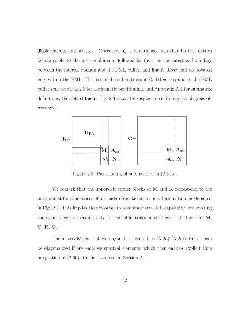
displacements and stresses. Moreover, uh is partitioned such that its first entries
belong solely to the interior domain, followed by those on the interface boundary
between the interior domain and the PML buffer, and finally those that are located
only within the PML. The rest of the submatrices in (2.31) correspond to the PML
buffer zone (see Fig. 2.3 for a schematic partitioning, and Appendix A.1 for submatrix
definitions; the dotted line in Fig. 2.3 separates displacement from stress degrees-of-
freedom).
Figure 2.3: Partitioning of submatrices in (2.31b).
We remark that the upper-left corner blocks of M and K correspond to the
mass and stiffness matrices of a standard displacement-only formulation, as depicted
in Fig. 2.3. This implies that in order to accommodate PML capability into existing
codes, one needs to account only for the submatrices on the lower-right blocks of M,
C, K, G.
The matrix M has a block-diagonal structure (see (A.2a)-(A.2c)); thus, it can
be diagonalized if one employs spectral elements, which then enables explicit time
integration of (2.30): this is discussed in Section 2.4.
32
Notice that the semi-discrete form (2.30) is not symmetric. In fact, a block-
diagonal structure for M comes at the price of losing symmetry. Alternatively, one
may preserve symmetry of the matrices in the semi-discrete form at the expense of
losing the block-diagonal form ofM, and thus the ability for explicit time integration.
We discuss this alternative formulation in Section 2.5.
2.3.2 Discretization in time
In this section, we discuss various possibilities of integrating the semi-discrete
form (2.30) in time. One may apply a time-marching scheme directly to (2.30), which
is third-order in time, or, exploit a more common scheme by first expressing (2.30)
as a second- or first-order in time system, via the introduction of auxiliary vectors.
Time-integration can be accomplished by working with either (2.30) or one of
its second- or first-order system counterparts, or, alternatively, one may (analytically)
integrate (2.30) in time first, to obviate the temporal differentiation of the forcing
vector. Assuming the system is initially at rest, there results
Md+Cd+Kd+Gd = f , (2.32a)
d =
∫ t
0
d(τ)|PML dτ, (2.32b)
where d is the vector of history terms. Equation (2.32) can be integrated via an
extended Newmark method as outlined in Appendix B.2. The scheme is implicit and
requires matrix factorization.
33
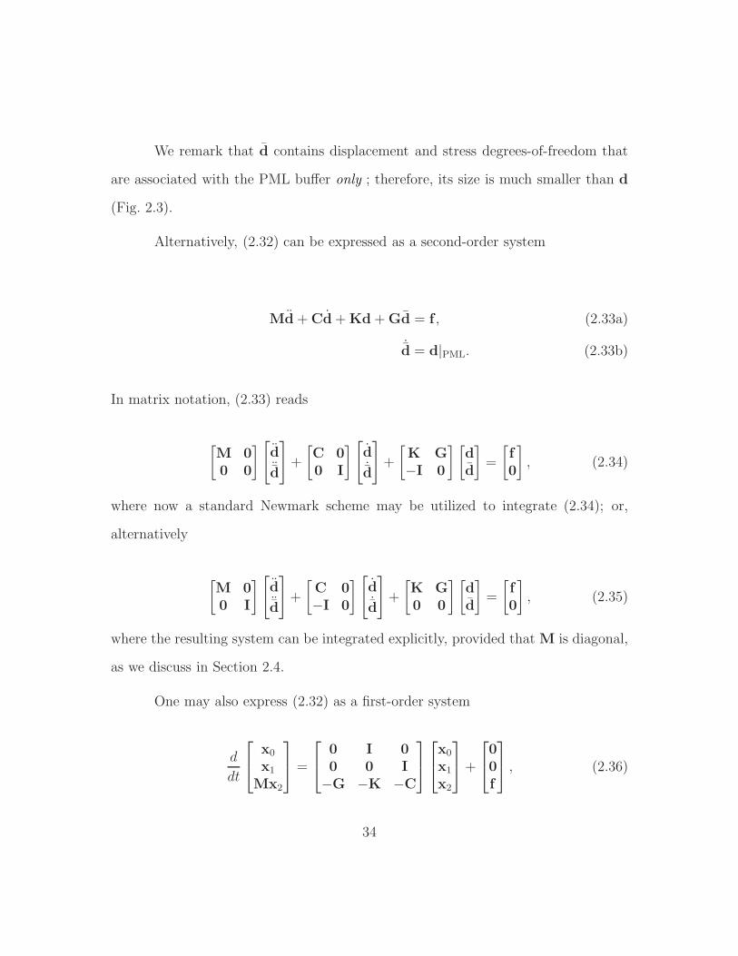
We remark that d contains displacement and stress degrees-of-freedom that
are associated with the PML buffer only ; therefore, its size is much smaller than d
(Fig. 2.3).
Alternatively, (2.32) can be expressed as a second-order system
Md+Cd+Kd+Gd = f , (2.33a)
˙d = d|PML. (2.33b)
In matrix notation, (2.33) reads
[M 00 0
][d¨d
]+
[C 00 I
] [d˙d
]+
[K G−I 0
] [dd
]=
[f0
], (2.34)
where now a standard Newmark scheme may be utilized to integrate (2.34); or,
alternatively
[M 00 I
][d¨d
]+
[C 0−I 0
] [d˙d
]+
[K G0 0
] [dd
]=
[f0
], (2.35)
where the resulting system can be integrated explicitly, provided that M is diagonal,
as we discuss in Section 2.4.
One may also express (2.32) as a first-order system
d
dt
x0
x1
Mx2
=
0 I 00 0 I−G −K −C
x0
x1
x2
+
00f
, (2.36)
34
where x0 = d, x1 = d, and x2 = d. Various standard explicit schemes could
then be used, provided that M is diagonal [74]. Here, we favor an explicit fourth-
order Runge-Kutta (RK-4) method. Based on various numerical experiments we
performed, we found out that, for the RK-4, ∆t < 0.8∆xcp
ensures stability on uniform
grids, where ∆x is the minimum distance between two grid points, and cp is the
maximum compressional wave velocity over an element. If, for a certain choice of
time step, a simulation with displacement-only finite elements is stable, then, the
associated simulation involving the PML is also stable with the same time step. In
other words, the introduction of the PML does not impose a more onerous time step
choice than an interior elastodynamics problem would require.
2.4 Spectral elements and explicit time integration
Hyperbolic initial-value-problems are, in general, advanced in time by using
explicit methods [22, 75]. This obviates the need for “inverting” a large linear system,
typically encountered in implicit schemes. Moreover, explicit schemes naturally lend
themselves to parallel computation, which is essential when dealing with large-scale
simulations in three-dimensional problems. In this section, we discuss how the matrix
M in the semi-discrete form (2.30) may be diagonalized, thus, enabling explicit time-
stepping via the techniques discussed in Section 2.3.2.
The simplest way of obtaining (discrete) diagonal mass-like matrices, is by
mass-lumping, as was done in [31, 76] where the authors used linear elements5. To
5By contrast to classical Galerkin finite elements, a finite difference formulation automaticallyyields diagonal mass-like matrices; see [74] for instance.
35
achieve high-order accuracy, however, one may use nodal spectral elements, where
numerical integration (quadrature rule) is based on the same nodes that polyno-
mial interpolation is carried out [77, 78]. This results in (discrete) diagonal mass-like
matrices, which are high-order accurate, depending on the degree of the interpolat-
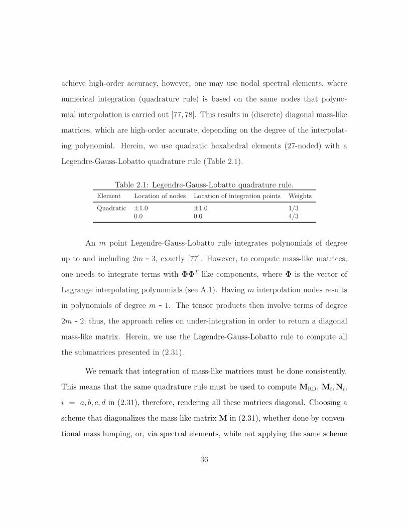
ing polynomial. Herein, we use quadratic hexahedral elements (27-noded) with a
Legendre-Gauss-Lobatto quadrature rule (Table 2.1).
Table 2.1: Legendre-Gauss-Lobatto quadrature rule.
Element Location of nodes Location of integration points Weights
Quadratic ±1.0 ±1.0 1/30.0 0.0 4/3
An m point Legendre-Gauss-Lobatto rule integrates polynomials of degree
up to and including 2m 3, exactly [77]. However, to compute mass-like matrices,
one needs to integrate terms with ΦΦT -like components, where Φ is the vector of
Lagrange interpolating polynomials (see A.1). Having m interpolation nodes results
in polynomials of degree m 1. The tensor products then involve terms of degree
2m 2; thus, the approach relies on under-integration in order to return a diagonal
mass-like matrix. Herein, we use the Legendre-Gauss-Lobatto rule to compute all
the submatrices presented in (2.31).
We remark that integration of mass-like matrices must be done consistently.
This means that the same quadrature rule must be used to compute MRD, Mi,Ni,
i = a, b, c, d in (2.31), therefore, rendering all these matrices diagonal. Choosing a
scheme that diagonalizes the mass-like matrix M in (2.31), whether done by conven-
tional mass lumping, or, via spectral elements, while not applying the same scheme
36
uniformly to all mass-like matrices, will result in instabilities, as it has also been
reported in [31, 79].
2.5 A symmetric formulation
In Section 2.2, we discussed a non-symmetric PML formulation that can be
integrated explicitly in time. In this section, we discuss an alternative formulation,
that results in a symmetric semi-discrete form, which would require an implicit time-
integration scheme due to a non-diagonal mass-like matrix. The key difference with
the Section 2.2 formulation is the handling of the combined constitutive and kine-
matic equations. To this end, we keep the equilibrium equation in (2.8a) intact, but
express (2.8b) in a different form.
Similar to what was done in [57], we start with the constitutive and kinematic
equations in the time domain
S = C[E], (2.37a)
E =1
2
[∇u+ (∇u)T
], (2.37b)
where E is the strain tensor, and C is the fourth-order constitutive tensor. For an
isotropic medium, C[E] = 2µE + λ(trE)I. Taking the Fourier transform of (2.37),
there results:
37
S = C[E], (2.38a)
E =1
2
[∇u+ (∇u)T
]. (2.38b)
Writing (2.38b) in the stretched coordinate system and using (2.4), we obtain:
E =1
2
(∇u)
1λx
0 0
0 1λy
0
0 0 1λz
+
1λx
0 0
0 1λy
0
0 0 1λz
(∇u)T
. (2.39)
Multiplying (2.39) by λxλyλz results in
λxλyλzE =1
2
[(∇u)Λ + Λ(∇u)T
]. (2.40)
Multiplying (2.40) by (iω)2 and using (2.13) and (2.2), we obtain
(iω)2aE+ iωbE+ cE+1
iωdE =
1
2(iω)2
[(∇u)Λe + Λe(∇u)T
]
+1
2iω
[(∇u)Λp + Λp(∇u)T
]+
1
2
[(∇u)Λw + Λw(∇u)T
]. (2.41)
Equation (2.41) constitutes the corresponding frequency-domain kinematic
equation in the stretched coordinate system. Taking the inverse Fourier transform
of (2.38a) and (2.41), there results
38
S = C[E], (2.42a)
aE+ bE + cE+ d
(∫ t
0
Edτ
)=
1
2
[(∇u)Λe + Λe(∇u)T + (∇u)Λp + Λp(∇u)T + (∇u)Λw + Λw(∇u)T
]. (2.42b)
Combining the resulting constitutive equation (2.42a) with the kinematic
equation (2.42b), and using the auxiliary variables introduced in (2.22), we obtain
D
[(a...S+ bS+ cS+ dS
)]=
1
2
[(∇u)Λe + Λe(∇u)T + (∇u)Λp + Λp(∇u)T + (∇u)Λw + Λw(∇u)T
], (2.43)
where D is the compliance tensor (E = D[S]). Equation (2.43) constitutes the PML
combined constitutive and kinematic equations, which is equivalent to (2.23b).
Next, similar to what we did in Section 2.3.1, we take the inner product of
(2.43) with (tensor) test function T(x) ∈ L2(Ω); there results:
∫
ΩPML
T :D(a...S+ bS+ cS+ dS
)dΩ
=1
2
∫
ΩPML
T :[(∇u)Λe + Λe(∇u)T + (∇u)Λp + Λp(∇u)T + (∇u)Λw + Λw(∇u)T
]dΩ.
(2.44)
Upon discretization of (2.26a) and (2.44) via (2.28)-(2.29), we obtain a semi-discrete
form
39
Ms
...d+Csd+Ksd+Gsd = f , (2.45)
with the following definition for system matrices
Ms =
[MRD + Ma 0
0 −Na
], Cs =
[Mb Ae
ATe −Nb
], (2.46a)
Ks =
[KRD + Mc Ap
ATp −Nc
], Gs =
[Md Aw
ATw −Nd
], (2.46b)
d =[uh Sh
]T, f =
[fRD 0
]T, (2.46c)
where a bar denotes matrix extension to encompass all the displacement degrees-of-
freedom; Mi, i = a, b, c, d are PML matrices defined in (A.2b), and Ni, i = a, b, c, d,
Ai, i = e, p, w are defined in (A.7) and (A.8), respectively. Moreover, similar to
what we did in Section 2.3.2, (2.45) can be expressed similarly to (2.32) by taking
into account (2.32b), therefore, obviating the temporal differentiation of the forcing
term:
Msd+Csd+Ksd+Gsd = f . (2.47)
System matrices defined in (2.46a)-(2.46b) are now symmetric and indefinite
by contrast to (2.31a)-(2.31b). They can become positive definite if one multiplies
their lower blocks by a minus sign, at the expense of losing symmetry. We refer to
[33, 80] for details.
40
We remark that Na in M is a block penta-diagonal matrix; this entails an
implicit time-integration scheme for the semi-discrete form. The extended Newmark
method outlined in Appendix B.2 could then be used for time-stepping, which then
necessitates factorization of a symmetric matrix.
2.6 Generalization for multi-axial perfectly-matched-layers
The aforementioned derivations are based on using the classical stretching
function (2.2), where stretching is enforced only in the direction perpendicular to
the PML interface. It has been reported that, in two dimensions, and under cer-
tain parameterizations, this stretching function creates spurious growths when waves
travel along the interface, thus leading to numerical instability. In an attempt to sta-
bilize the PML (in 2D), Meza-Fajardo and Papageorgiou [41] proposed coordinate-
stretching in all directions within the PML buffer, leading to the, so-called, multi-
axial PML (M-PML).
Herein, we show that by making minimal modifications, our framework can
also accommodate the M-PML. We focus on the “right” PML buffer zone first, i.e.,
the volume contained in x0 ≤ x ≤ xt (see Fig. 2.1 with s replaced by x); extending
the ideas to the zones where two or three layers intersect is straightforward, and
can be accomplished by using superposition. We stretch the physical coordinates
according to
41
x = x0 +
∫ x
x0
[αx(x
′) +1
iωβx(x
′)
]dx′, (2.48a)
y = y0 +
∫ y
y0
[αy(x) +
1
iωβy(x)
]dy′, (2.48b)
z = z0 +
∫ z
z0
[αz(x) +
1
iωβz(x)
]dz′. (2.48c)
where αy, αz, βy, and βz are functions of x only, and are defined as
αy(x) = 1 + αo
[(x− xo)nx
LPML
]m, βy(x) = βx(x), (2.49a)
αz(x) = 1 + αo
[(x− xo)nx
LPML
]m, βz(x) = βx(x), (2.49b)
where is a proportionality constant, and nx is the outward unit normal at the
interface, similar to ns in Fig. 2.1; αx and βx are defined in (2.5). We remark that
αy, αz would have been reduced to one, and βy, βz would have been identically zero,
in the right buffer, had we used the classical stretching. Applying the fundamental
theorem of calculus to (2.48), results in
λx :=∂x
∂x= αx(x) +
1
iωβx(x), (2.50a)
λy :=∂y
∂y= αy(x) +
1
iωβy(x), (2.50b)
λz :=∂z
∂z= αz(x) +
1
iωβz(x). (2.50c)
These are the stretching functions the authors used in [45]. However, the definition
of the stretched gradient operator in equation (3) in [45] requires additional terms,
42
which the authors had not included. For example, the derivative with respect to x
should read
∂( )
∂x=
∂( )
∂x
∂x
∂x+
∂( )
∂y
∂y
∂x+
∂( )
∂z
∂z
∂x(2.51a)
=1
λx
∂( )
∂x− λyx
λxλy
∂( )
∂y− λzx
λxλz
∂( )
∂z, (2.51b)
instead of the expression given in [45], which reads
∂( )
∂x=
1
λx
∂( )
∂x. (2.52a)
In (2.51) above, the cross-derivative terms are defined as
λyx :=∂y
∂x=
(∂
∂xαy(x) +
1
iω
∂
∂xβy(x)
)(y − y0), (2.53a)
λzx :=∂z
∂x=
(∂
∂xαz(x) +
1
iω
∂
∂xβz(x)
)(z − z0). (2.53b)
In other words, it seems that in [41, 45], the authors have not accounted prop-
erly for the Jacobian. Thus, there are at least two possible forms of the M-PML: the
uncorrected form in [41, 45], and the corrected form, which accounts for the cross-
derivatives. Interestingly, numerical experiments we performed in two dimensions
with the corrected form yielded small, but non-negligible reflections from the inter-
face. By contrast, the uncorrected form yielded better results, despite its unsound
mathematical foundation. This has led us to adopt the approach taken in [41, 45];
accordingly, the equation pertaining to the conservation of linear momentum in the
stretched coordinate system becomes
43
div(STΛ
)− ST divΛ = (iω)2ρ λxλyλz u, (2.54)
which results in the following strong form
div(STΛe + STΛp + STΛw
)−
(ST divΛe + ST divΛp + ST divΛw
)
= ρ (a...u+ bu+ cu+ du) . (2.55)
The structure of the formulation pertaining to the combined constitutive and
kinematic equation in the stretched coordinate system we previously discussed re-
mains unaltered. Hence, for accommodating the M-PML, one only needs to replace
(2.24b) in the strong form of the equations with (2.55), which, in turn, changes the
definition of submatrices Aeu,Apu, and Awu in (2.31). The new definition of these
submatrices for the M-PML case are given in Appendix A.3.
2.7 Numerical Experiments
We present three numerical experiments to test the accuracy and efficacy
of our hybrid formulation. The first example involves a homogeneous half-space;
the second one is a horizontally layered medium with an ellipsoidal inclusion. The
last example compares various formulations discussed in Sections 2.3.2 and 2.5. We
compare our results against an enlarged domain6 solution with fixed boundaries,
obtained via a standard displacement-only formulation, which may be viewed as
6denoted by ΩED, such that ΩRD ⊂ ΩED.
44
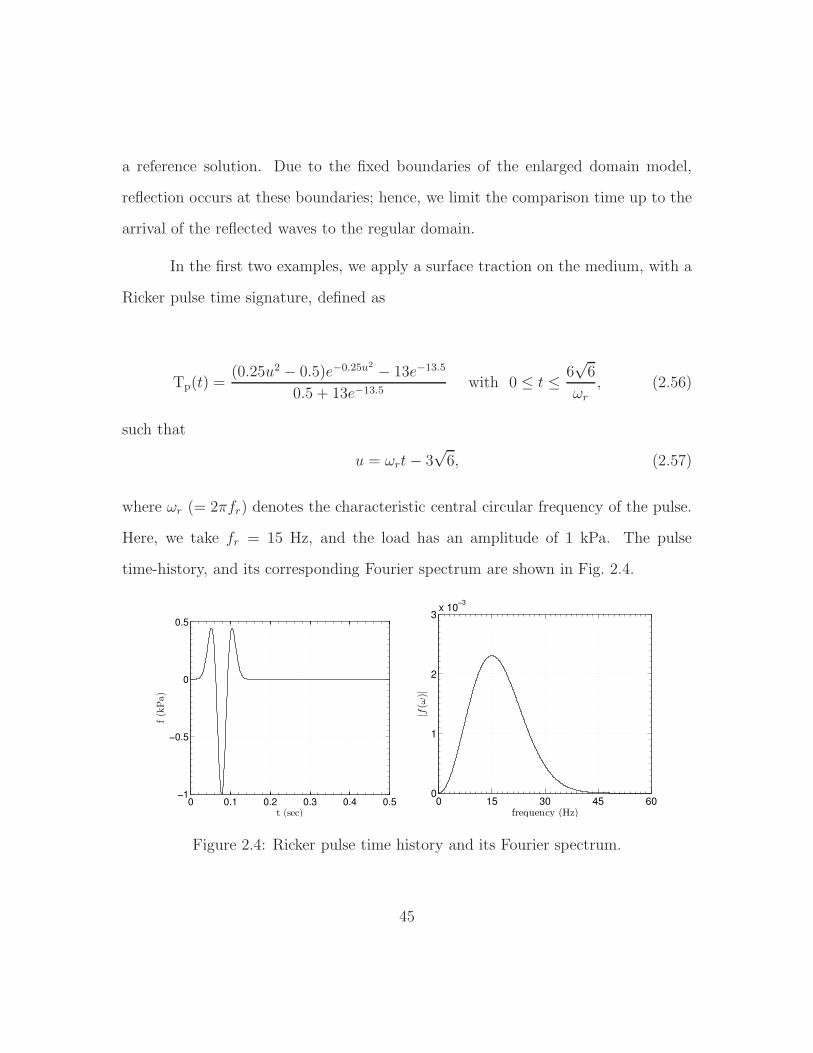
a reference solution. Due to the fixed boundaries of the enlarged domain model,
reflection occurs at these boundaries; hence, we limit the comparison time up to the
arrival of the reflected waves to the regular domain.
In the first two examples, we apply a surface traction on the medium, with a
Ricker pulse time signature, defined as
Tp(t) =(0.25u2 − 0.5)e−0.25u2 − 13e−13.5
0.5 + 13e−13.5with 0 ≤ t ≤ 6
√6
ωr, (2.56)
such that
u = ωrt− 3√6, (2.57)
where ωr (= 2πfr) denotes the characteristic central circular frequency of the pulse.
Here, we take fr = 15 Hz, and the load has an amplitude of 1 kPa. The pulse
time-history, and its corresponding Fourier spectrum are shown in Fig. 2.4.
0 0.1 0.2 0.3 0.4 0.5−1
−0.5
0
0.5
t (sec)
f(k
Pa)
0 15 30 45 600
1
2
3x 10
−3
frequency (Hz)
|f(ω
)|
Figure 2.4: Ricker pulse time history and its Fourier spectrum.
45

In order to quantify the performance of our PML formulation, we consider two met-
rics: (a) time-history comparisons at select nodes via evaluation of a time-dependent
Euclidean norm of the error, relative to the reference solution; and (b) decay of the
total energy within the regular domain.
We define the time-dependent Euclidean norm of the relative error at a point
x ∈ ΩRD as
e(x, t) =‖u(x, t)− uED(x, t)‖2
maxt‖uED(x, t)‖2
, (2.58)
where uED(x, t) represents the enlarged domain solution, and the Euclidean norm of
a vector u(x, t) = [ux(x, t), uy(x, t), uz(x, t)]T is defined as
‖u(x, t)‖2 =√(
ux(x, t))2
+(uy(x, t)
)2+(uz(x, t)
)2. (2.59)
The energy introduced into the system through the loading is carried via
waves, which then enter the PML buffer and attenuate. Therefore, an effective PML
ought to result in the rapid decay of energy. The total energy of the system can be
computed at any time via
Et(t) =1
2
∫
ΩRD
ρ(x)[uT (x, t)u(x, t)
]dΩ +
1
2
∫
ΩRD
[σT (x, t)ǫ(x, t)
]dΩ, (2.60)
where u denotes the velocity vector, and σ and ǫ are stress and strain vectors, respec-
tively. We compute and compare energy only within the regular domain. Moreover,
46
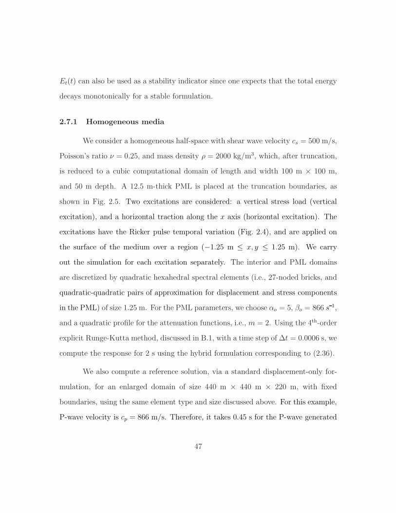
Et(t) can also be used as a stability indicator since one expects that the total energy
decays monotonically for a stable formulation.
2.7.1 Homogeneous media
We consider a homogeneous half-space with shear wave velocity cs = 500 m/s,
Poisson’s ratio ν = 0.25, and mass density ρ = 2000 kg/m3, which, after truncation,
is reduced to a cubic computational domain of length and width 100 m × 100 m,
and 50 m depth. A 12.5 m-thick PML is placed at the truncation boundaries, as
shown in Fig. 2.5. Two excitations are considered: a vertical stress load (vertical
excitation), and a horizontal traction along the x axis (horizontal excitation). The
excitations have the Ricker pulse temporal variation (Fig. 2.4), and are applied on
the surface of the medium over a region (−1.25 m ≤ x, y ≤ 1.25 m). We carry
out the simulation for each excitation separately. The interior and PML domains
are discretized by quadratic hexahedral spectral elements (i.e., 27-noded bricks, and
quadratic-quadratic pairs of approximation for displacement and stress components
in the PML) of size 1.25 m. For the PML parameters, we choose αo = 5, βo = 866 s 1,
and a quadratic profile for the attenuation functions, i.e., m = 2. Using the 4th-order
explicit Runge-Kutta method, discussed in B.1, with a time step of ∆t = 0.0006 s, we
compute the response for 2 s using the hybrid formulation corresponding to (2.36).
We also compute a reference solution, via a standard displacement-only for-
mulation, for an enlarged domain of size 440 m × 440 m × 220 m, with fixed
boundaries, using the same element type and size discussed above. For this example,
P-wave velocity is cp = 866 m/s. Therefore, it takes 0.45 s for the P-wave generated
47
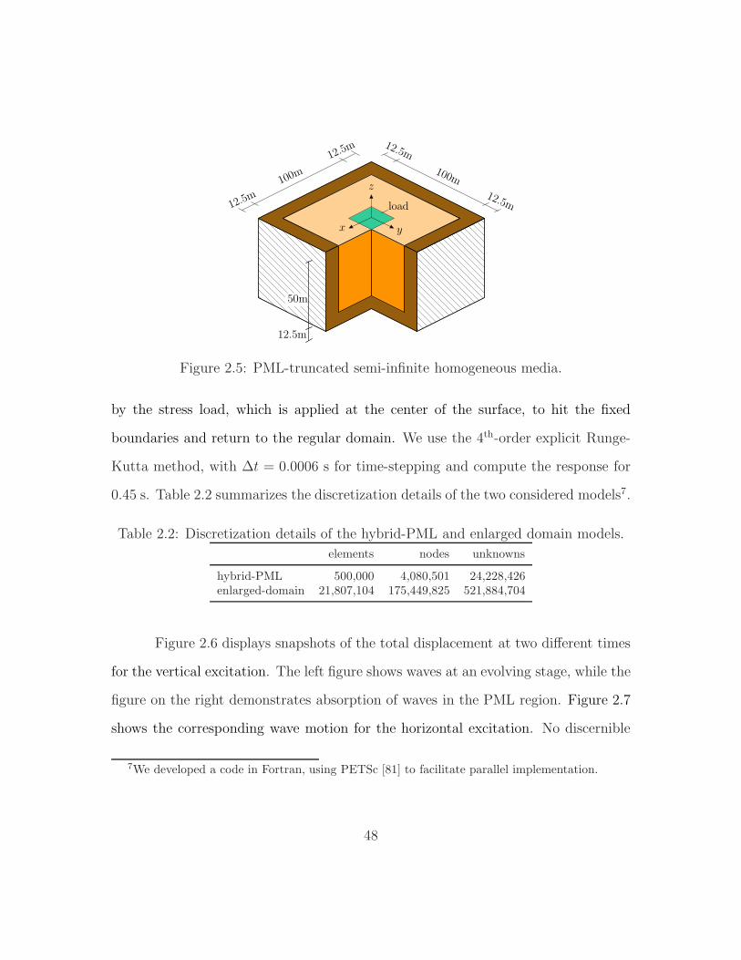
100m100m
x y
z
load
50m
Figure 2.5: PML-truncated semi-infinite homogeneous media.
by the stress load, which is applied at the center of the surface, to hit the fixed
boundaries and return to the regular domain. We use the 4th-order explicit Runge-
Kutta method, with ∆t = 0.0006 s for time-stepping and compute the response for
0.45 s. Table 2.2 summarizes the discretization details of the two considered models7.
Table 2.2: Discretization details of the hybrid-PML and enlarged domain models.
elements nodes unknowns
hybrid-PML 500,000 4,080,501 24,228,426enlarged-domain 21,807,104 175,449,825 521,884,704
Figure 2.6 displays snapshots of the total displacement at two different times
for the vertical excitation. The left figure shows waves at an evolving stage, while the
figure on the right demonstrates absorption of waves in the PML region. Figure 2.7
shows the corresponding wave motion for the horizontal excitation. No discernible
7We developed a code in Fortran, using PETSc [81] to facilitate parallel implementation.
48
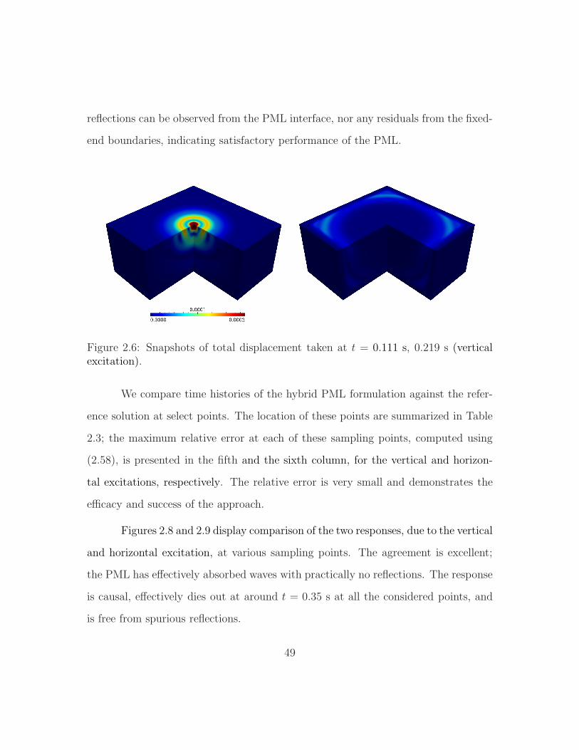
reflections can be observed from the PML interface, nor any residuals from the fixed-
end boundaries, indicating satisfactory performance of the PML.
Figure 2.6: Snapshots of total displacement taken at t = 0.111 s, 0.219 s (verticalexcitation).
We compare time histories of the hybrid PML formulation against the refer-
ence solution at select points. The location of these points are summarized in Table
2.3; the maximum relative error at each of these sampling points, computed using
(2.58), is presented in the fifth and the sixth column, for the vertical and horizon-
tal excitations, respectively. The relative error is very small and demonstrates the
efficacy and success of the approach.
Figures 2.8 and 2.9 display comparison of the two responses, due to the vertical
and horizontal excitation, at various sampling points. The agreement is excellent;
the PML has effectively absorbed waves with practically no reflections. The response
is causal, effectively dies out at around t = 0.35 s at all the considered points, and
is free from spurious reflections.
49
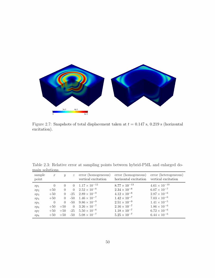
0 6e-5
2e-5 4e-5
Figure 2.7: Snapshots of total displacement taken at t = 0.147 s, 0.219 s (horizontalexcitation).
Table 2.3: Relative error at sampling points between hybrid-PML and enlarged do-main solutions.sample x y z error (homogeneous) error (homogeneous) error (heterogeneous)point vertical excitation horizontal excitation vertical excitation
sp1 0 0 0 1.17× 10⁻¹² 8.77× 10⁻¹³ 4.61× 10⁻¹⁰
sp2 +50 0 0 2.52× 10⁻⁸ 2.34× 10⁻⁸ 6.07× 10⁻⁷
sp3 +50 0 -25 2.89× 10⁻⁹ 4.12× 10⁻⁸ 2.87× 10⁻⁶
sp4 +50 0 -50 1.46× 10⁻⁷ 1.42× 10⁻⁷ 7.03× 10⁻⁶
sp5 0 0 -50 9.86× 10⁻⁹ 2.51× 10⁻⁹ 1.41× 10⁻⁵
sp6 +50 +50 0 3.26× 10⁻⁷ 2.16× 10⁻⁷ 1.86× 10⁻⁶
sp7 +50 +50 -25 5.50× 10⁻⁸ 1.18× 10⁻⁷ 6.72× 10⁻⁶
sp8 +50 +50 -50 5.08× 10⁻⁷ 5.25× 10⁻⁷ 6.44× 10⁻⁶
50
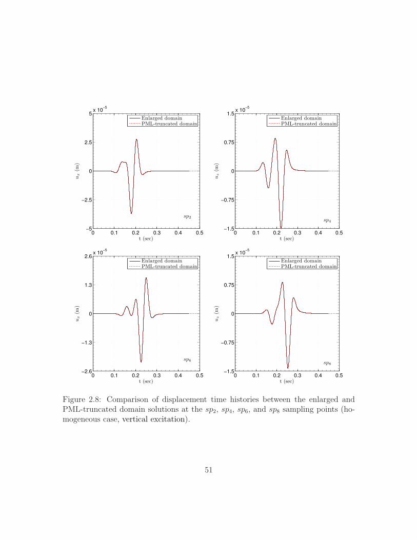
0 0.1 0.2 0.3 0.4 0.5−5
−2.5
0
2.5
5x 10
−5
t (sec)
ux
(m)
sp2
Enlarged domainPML-truncated domain
0 0.1 0.2 0.3 0.4 0.5−1.5
−0.75
0
0.75
1.5x 10
−5
t (sec)
uz
(m)
sp4
Enlarged domainPML-truncated domain
0 0.1 0.2 0.3 0.4 0.5−2.6
−1.3
0
1.3
2.6x 10
−5
t (sec)
ux
(m)
sp6
Enlarged domainPML-truncated domain
0 0.1 0.2 0.3 0.4 0.5−1.5
−0.75
0
0.75
1.5x 10
−5
t (sec)
uz
(m)
sp8
Enlarged domainPML-truncated domain
Figure 2.8: Comparison of displacement time histories between the enlarged andPML-truncated domain solutions at the sp2, sp4, sp6, and sp8 sampling points (ho-mogeneous case, vertical excitation).
51
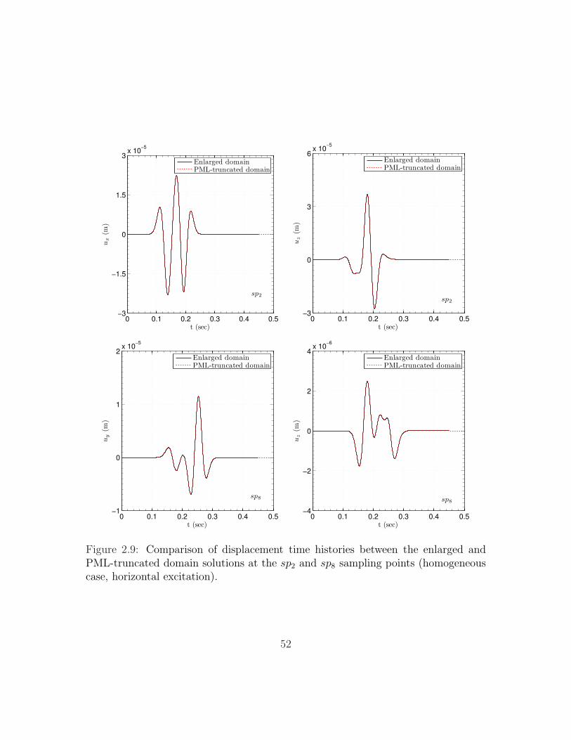
0 0.1 0.2 0.3 0.4 0.5−3
−1.5
0
1.5
3x 10
−5
t (sec)
ux
(m)
sp2
Enlarged domainPML-truncated domain
0 0.1 0.2 0.3 0.4 0.5−3
0
3
6x 10
−5
t (sec)
uz
(m)
sp2
Enlarged domainPML-truncated domain
0 0.1 0.2 0.3 0.4 0.5−1
0
1
2x 10
−5
t (sec)
uy
(m)
sp8
Enlarged domainPML-truncated domain
0 0.1 0.2 0.3 0.4 0.5−4
−2
0
2
4x 10
−6
t (sec)
uz
(m)
sp8
Enlarged domainPML-truncated domain
Figure 2.9: Comparison of displacement time histories between the enlarged andPML-truncated domain solutions at the sp2 and sp8 sampling points (homogeneouscase, horizontal excitation).
52
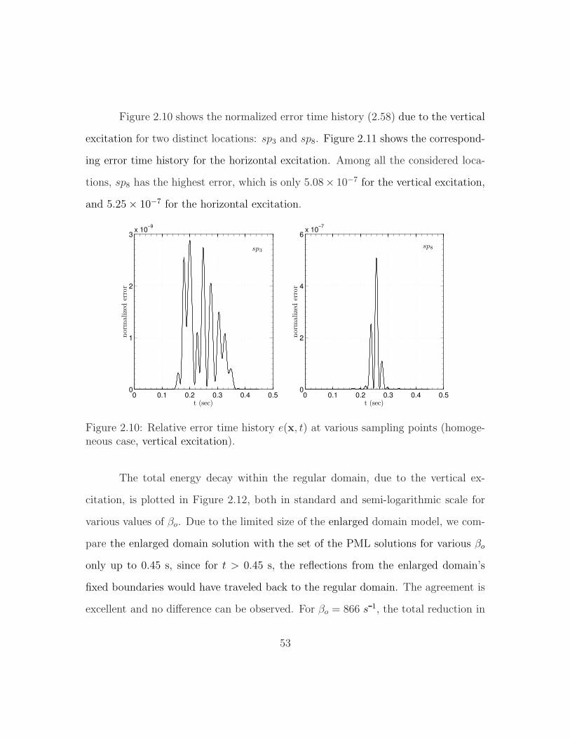
Figure 2.10 shows the normalized error time history (2.58) due to the vertical
excitation for two distinct locations: sp3 and sp8. Figure 2.11 shows the correspond-
ing error time history for the horizontal excitation. Among all the considered loca-
tions, sp8 has the highest error, which is only 5.08× 10⁻⁷ for the vertical excitation,
and 5.25× 10⁻⁷ for the horizontal excitation.
0 0.1 0.2 0.3 0.4 0.50
1
2
3x 10
−9
t (sec)
norm
alize
der
ror
sp3
0 0.1 0.2 0.3 0.4 0.50
2
4
6x 10
−7
t (sec)
norm
alize
der
ror
sp8
Figure 2.10: Relative error time history e(x, t) at various sampling points (homoge-neous case, vertical excitation).
The total energy decay within the regular domain, due to the vertical ex-
citation, is plotted in Figure 2.12, both in standard and semi-logarithmic scale for
various values of βo. Due to the limited size of the enlarged domain model, we com-
pare the enlarged domain solution with the set of the PML solutions for various βo
only up to 0.45 s, since for t > 0.45 s, the reflections from the enlarged domain’s
fixed boundaries would have traveled back to the regular domain. The agreement is
excellent and no difference can be observed. For βo = 866 s 1, the total reduction in
53
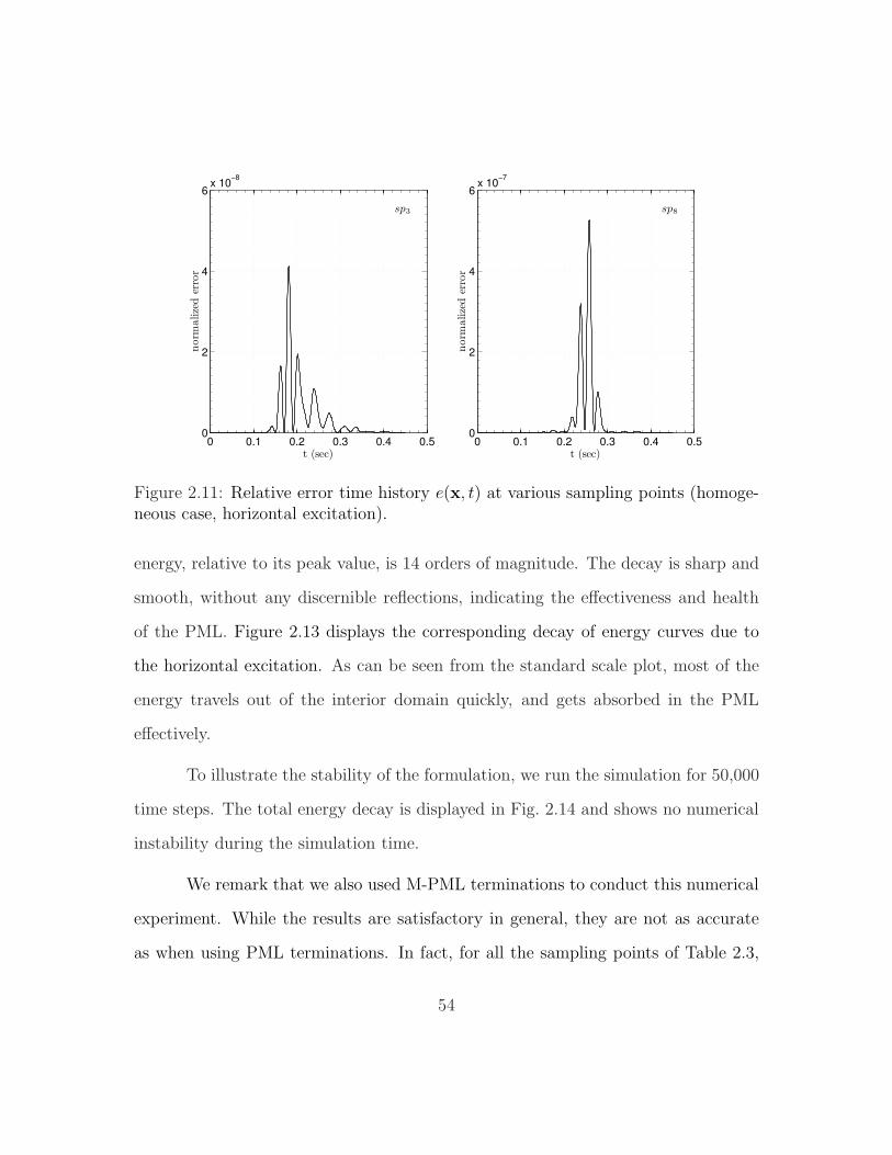
0 0.1 0.2 0.3 0.4 0.50
2
4
6x 10
−8
t (sec)
norm
alize
der
ror
sp3
0 0.1 0.2 0.3 0.4 0.50
2
4
6x 10
−7
t (sec)norm
alize
der
ror
sp8
Figure 2.11: Relative error time history e(x, t) at various sampling points (homoge-neous case, horizontal excitation).
energy, relative to its peak value, is 14 orders of magnitude. The decay is sharp and
smooth, without any discernible reflections, indicating the effectiveness and health
of the PML. Figure 2.13 displays the corresponding decay of energy curves due to
the horizontal excitation. As can be seen from the standard scale plot, most of the
energy travels out of the interior domain quickly, and gets absorbed in the PML
effectively.
To illustrate the stability of the formulation, we run the simulation for 50,000
time steps. The total energy decay is displayed in Fig. 2.14 and shows no numerical
instability during the simulation time.
We remark that we also used M-PML terminations to conduct this numerical
experiment. While the results are satisfactory in general, they are not as accurate
as when using PML terminations. In fact, for all the sampling points of Table 2.3,
54
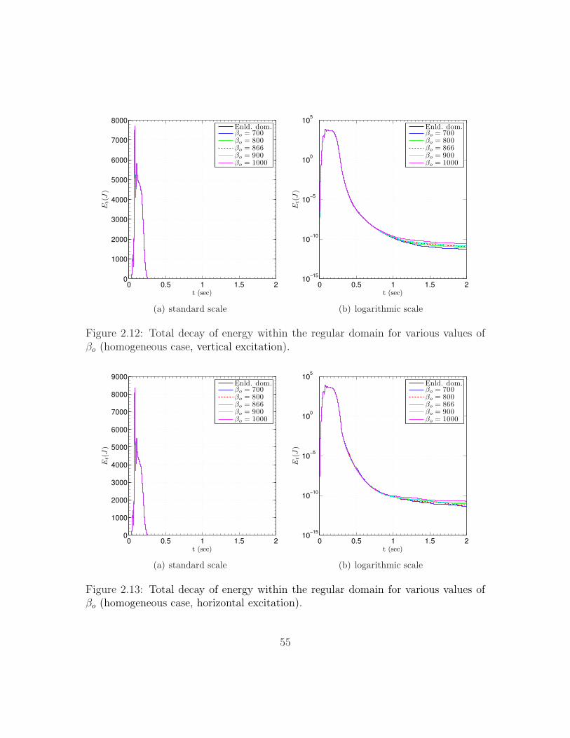
0 0.5 1 1.5 20
1000
2000
3000
4000
5000
6000
7000
8000
t (sec)
Et(J
)
Enld. dom.βo = 700βo = 800βo = 866βo = 900βo = 1000
(a) standard scale
0 0.5 1 1.5 210
−15
10−10
10−5
100
105
t (sec)E
t(J
)
Enld. dom.βo = 700βo = 800βo = 866βo = 900βo = 1000
(b) logarithmic scale
Figure 2.12: Total decay of energy within the regular domain for various values ofβo (homogeneous case, vertical excitation).
0 0.5 1 1.5 20
1000
2000
3000
4000
5000
6000
7000
8000
9000
t (sec)
Et(J
)
Enld. dom.βo = 700βo = 800βo = 866βo = 900βo = 1000
(a) standard scale
0 0.5 1 1.5 210
−15
10−10
10−5
100
105
t (sec)
Et(J
)
Enld. dom.βo = 700βo = 800βo = 866βo = 900βo = 1000
(b) logarithmic scale
Figure 2.13: Total decay of energy within the regular domain for various values ofβo (homogeneous case, horizontal excitation).
55
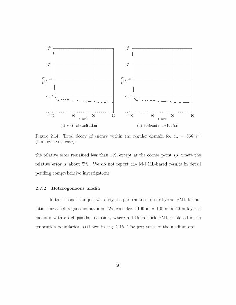
0 10 20 3010
−15
10−10
10−5
100
105
t (sec)
Et(J
)
(a) vertical excitation
0 10 20 3010
−15
10−10
10−5
100
105
t (sec)E
t(J
)
(b) horizontal excitation
Figure 2.14: Total decay of energy within the regular domain for βo = 866 s 1
(homogeneous case).
the relative error remained less than 1%, except at the corner point sp8 where the
relative error is about 5%. We do not report the M-PML-based results in detail
pending comprehensive investigations.
2.7.2 Heterogeneous media
In the second example, we study the performance of our hybrid-PML formu-
lation for a heterogeneous medium. We consider a 100 m × 100 m × 50 m layered
medium with an ellipsoidal inclusion, where a 12.5 m-thick PML is placed at its
truncation boundaries, as shown in Fig. 2.15. The properties of the medium are
56
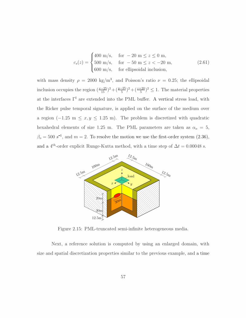
cs(z) =
400 m/s, for − 20 m ≤ z ≤ 0 m,
500 m/s, for − 50 m ≤ z < −20 m,
600 m/s, for ellipsoidal inclusion,
(2.61)
with mass density ρ = 2000 kg/m3, and Poisson’s ratio ν = 0.25; the ellipsoidal
inclusion occupies the region (x−2515
)2+(y−255
)2+( z+205
)2 ≤ 1. The material properties
at the interfaces ΓI are extended into the PML buffer. A vertical stress load, with
the Ricker pulse temporal signature, is applied on the surface of the medium over
a region (−1.25 m ≤ x, y ≤ 1.25 m). The problem is discretized with quadratic
hexahedral elements of size 1.25 m. The PML parameters are taken as αo = 5,
βo = 500 s 1, and m = 2. To resolve the motion we use the first-order system (2.36),
and a 4th-order explicit Runge-Kutta method, with a time step of ∆t = 0.00048 s.
100m10
0m
x y
z
load
20m
30m
30m
Figure 2.15: PML-truncated semi-infinite heterogeneous media.
Next, a reference solution is computed by using an enlarged domain, with
size and spatial discretization properties similar to the previous example, and a time
57
step of ∆t = 0.00048 s. Table 2.2 summarizes the spatial discretization details of the
problem.
To assess the performance of our hybrid PML formulation, we compare dis-
placement time histories at select locations against the enlarged domain solution.
The sampling points, with their corresponding relative error computed via (2.58) are
summarized in the last column of Table 2.3. The relative error values are higher than
the previous example, which was a homogeneous medium, but still, they are very
low. In fact, the highest relative error, which corresponds to sp8, is only 1.41×10⁻⁵,
which is very small in practical applications.
Snapshots of the total displacement at two different times are displayed in
Fig. 2.16. The figure on the left shows waves at an evolving stage, while the right
figure indicates absorption of waves in the PML buffer zone. Notice that no dis-
cernible reflections can be seen from the PML interfaces, nor any residuals from the
fixed-end boundaries, a visual indication of satisfactory performance of the PML
for domains involving heterogeneous material properties. Figure 2.17 depicts the
complex wave pattern around the ellipsoidal inclusion on a cross-section through the
domain situated at 20 m from the surface going through the ellipsoid’s midplane.
Various components of displacement time-histories for the enlarged domain
and the hybrid PML simulations are displayed in Fig. 2.18 for select sampling points.
The agreement is excellent. The response effectively dies out at around 0.45 s.
The relative error time histories are shown in Fig. 2.19 and indicate satisfactory
performance of the PML.
58
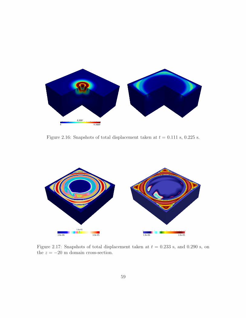
Figure 2.16: Snapshots of total displacement taken at t = 0.111 s, 0.225 s.
3.0e-06 3.0e-05
1.0e-05
1.0e-06 1.0e-05
Figure 2.17: Snapshots of total displacement taken at t = 0.233 s, and 0.290 s, onthe z = −20 m domain cross-section.
59
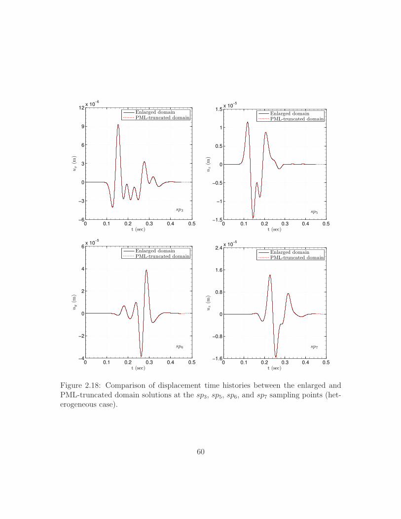
0 0.1 0.2 0.3 0.4 0.5−6
−3
0
3
6
9
12x 10
−6
t (sec)
ux
(m)
sp3
Enlarged domainPML-truncated domain
0 0.1 0.2 0.3 0.4 0.5−1.5
−1
−0.5
0
0.5
1
1.5x 10
−5
t (sec)
uz
(m)
sp5
Enlarged domainPML-truncated domain
0 0.1 0.2 0.3 0.4 0.5−4
−2
0
2
4
6x 10
−5
t (sec)
uy
(m)
sp6
Enlarged domainPML-truncated domain
0 0.1 0.2 0.3 0.4 0.5−1.6
−0.8
0
0.8
1.6
2.4x 10
−5
t (sec)
uz
(m)
sp7
Enlarged domainPML-truncated domain
Figure 2.18: Comparison of displacement time histories between the enlarged andPML-truncated domain solutions at the sp3, sp5, sp6, and sp7 sampling points (het-erogeneous case).
60
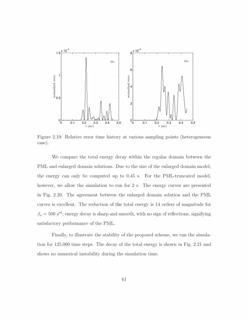
0 0.1 0.2 0.3 0.4 0.50
0.5
1
1.5x 10
−5
t (sec)
norm
alize
der
ror
sp5
0 0.1 0.2 0.3 0.4 0.50
2
4
6
8x 10
−6
t (sec)norm
alize
der
ror
sp8
Figure 2.19: Relative error time history at various sampling points (heterogeneouscase).
We compare the total energy decay within the regular domain between the
PML and enlarged domain solutions. Due to the size of the enlarged domain model,
the energy can only be computed up to 0.45 s. For the PML-truncated model,
however, we allow the simulation to run for 2 s. The energy curves are presented
in Fig. 2.20. The agreement between the enlarged domain solution and the PML
curves is excellent. The reduction of the total energy is 14 orders of magnitude for
βo = 500 s 1; energy decay is sharp and smooth, with no sign of reflections, signifying
satisfactory performance of the PML.
Finally, to illustrate the stability of the proposed scheme, we run the simula-
tion for 125,000 time steps. The decay of the total energy is shown in Fig. 2.21 and
shows no numerical instability during the simulation time.
61
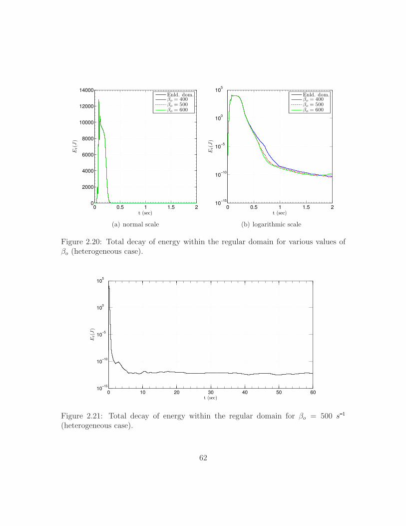
0 0.5 1 1.5 20
2000
4000
6000
8000
10000
12000
14000
t (sec)
Et(J
)
Enld. dom.βo = 400βo = 500βo = 600
(a) normal scale
0 0.5 1 1.5 210
−15
10−10
10−5
100
105
t (sec)E
t(J
)
Enld. dom.βo = 400βo = 500βo = 600
(b) logarithmic scale
Figure 2.20: Total decay of energy within the regular domain for various values ofβo (heterogeneous case).
0 10 20 30 40 50 6010
−15
10−10
10−5
100
105
t (sec)
Et(J
)
Figure 2.21: Total decay of energy within the regular domain for βo = 500 s 1
(heterogeneous case).
62
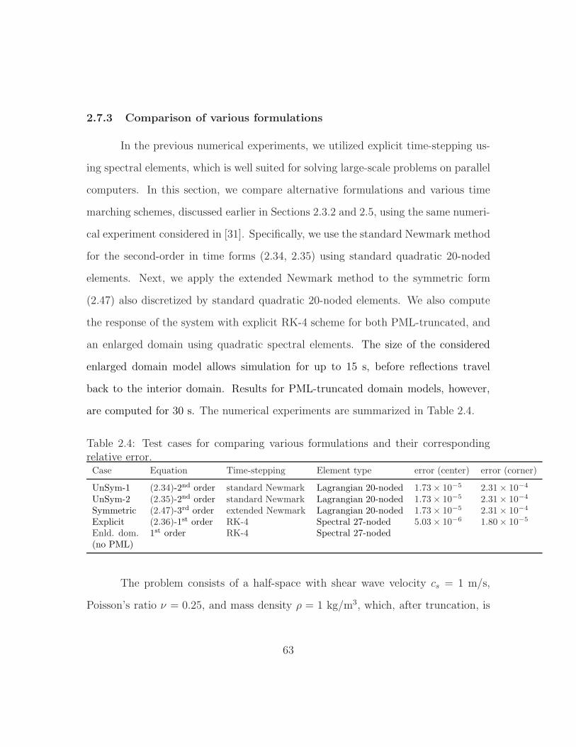
2.7.3 Comparison of various formulations
In the previous numerical experiments, we utilized explicit time-stepping us-
ing spectral elements, which is well suited for solving large-scale problems on parallel
computers. In this section, we compare alternative formulations and various time
marching schemes, discussed earlier in Sections 2.3.2 and 2.5, using the same numeri-
cal experiment considered in [31]. Specifically, we use the standard Newmark method
for the second-order in time forms (2.34, 2.35) using standard quadratic 20-noded
elements. Next, we apply the extended Newmark method to the symmetric form
(2.47) also discretized by standard quadratic 20-noded elements. We also compute
the response of the system with explicit RK-4 scheme for both PML-truncated, and
an enlarged domain using quadratic spectral elements. The size of the considered
enlarged domain model allows simulation for up to 15 s, before reflections travel
back to the interior domain. Results for PML-truncated domain models, however,
are computed for 30 s. The numerical experiments are summarized in Table 2.4.
Table 2.4: Test cases for comparing various formulations and their correspondingrelative error.Case Equation Time-stepping Element type error (center) error (corner)
UnSym-1 (2.34)-2nd order standard Newmark Lagrangian 20-noded 1.73× 10⁻⁵ 2.31× 10⁻⁴
UnSym-2 (2.35)-2nd order standard Newmark Lagrangian 20-noded 1.73× 10⁻⁵ 2.31× 10⁻⁴
Symmetric (2.47)-3rd order extended Newmark Lagrangian 20-noded 1.73× 10⁻⁵ 2.31× 10⁻⁴
Explicit (2.36)-1st order RK-4 Spectral 27-noded 5.03× 10⁻⁶ 1.80× 10⁻⁵
Enld. dom. 1st order RK-4 Spectral 27-noded(no PML)
The problem consists of a half-space with shear wave velocity cs = 1 m/s,
Poisson’s ratio ν = 0.25, and mass density ρ = 1 kg/m3, which, after truncation, is
63
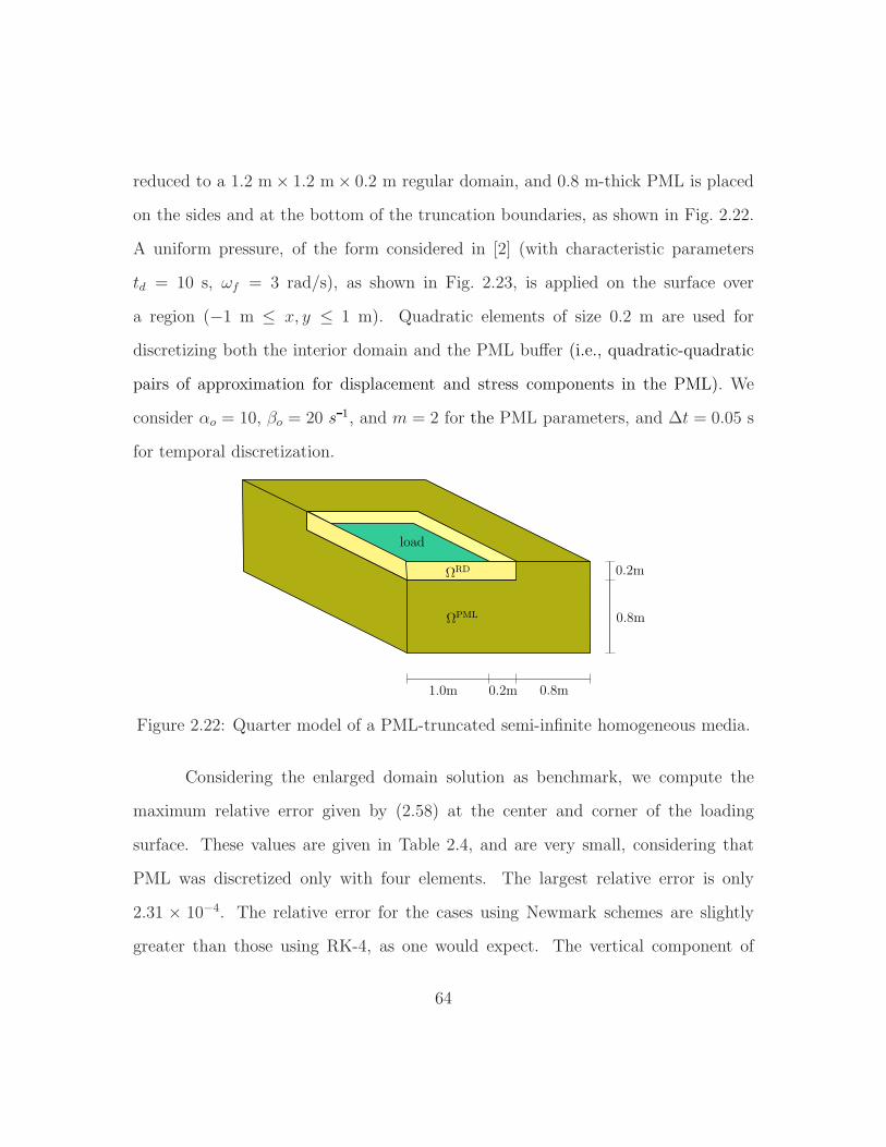
reduced to a 1.2 m× 1.2 m× 0.2 m regular domain, and 0.8 m-thick PML is placed
on the sides and at the bottom of the truncation boundaries, as shown in Fig. 2.22.
A uniform pressure, of the form considered in [2] (with characteristic parameters
td = 10 s, ωf = 3 rad/s), as shown in Fig. 2.23, is applied on the surface over
a region (−1 m ≤ x, y ≤ 1 m). Quadratic elements of size 0.2 m are used for
discretizing both the interior domain and the PML buffer (i.e., quadratic-quadratic
pairs of approximation for displacement and stress components in the PML). We
consider αo = 10, βo = 20 s 1, and m = 2 for the PML parameters, and ∆t = 0.05 s
for temporal discretization.
load
Figure 2.22: Quarter model of a PML-truncated semi-infinite homogeneous media.
Considering the enlarged domain solution as benchmark, we compute the
maximum relative error given by (2.58) at the center and corner of the loading
surface. These values are given in Table 2.4, and are very small, considering that
PML was discretized only with four elements. The largest relative error is only
2.31 × 10⁻⁴. The relative error for the cases using Newmark schemes are slightly
greater than those using RK-4, as one would expect. The vertical component of
64
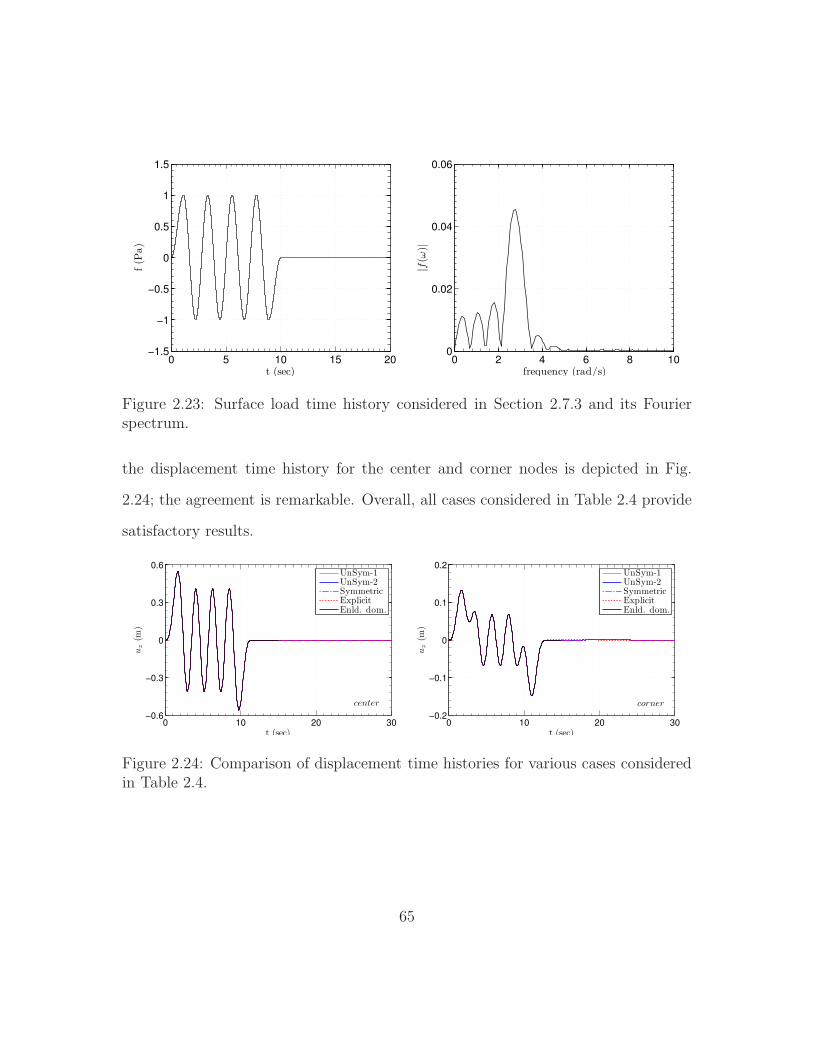
0 5 10 15 20−1.5
−1
−0.5
0
0.5
1
1.5
t (sec)
f(P
a)
0 2 4 6 8 100
0.02
0.04
0.06
frequency (rad/s)
|f(ω
)|
Figure 2.23: Surface load time history considered in Section 2.7.3 and its Fourierspectrum.
the displacement time history for the center and corner nodes is depicted in Fig.
2.24; the agreement is remarkable. Overall, all cases considered in Table 2.4 provide
satisfactory results.
0 10 20 30−0.6
−0.3
0
0.3
0.6
t (sec)
uz
(m)
center
UnSym-1UnSym-2SymmetricExplicitEnld. dom.
0 10 20 30−0.2
−0.1
0
0.1
0.2
t (sec)
uz
(m)
corner
UnSym-1UnSym-2SymmetricExplicitEnld. dom.
Figure 2.24: Comparison of displacement time histories for various cases consideredin Table 2.4.
65
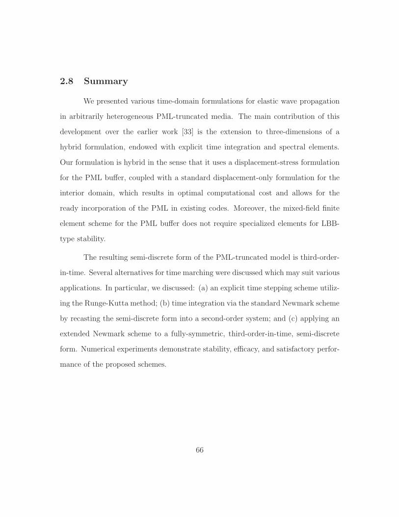
2.8 Summary
We presented various time-domain formulations for elastic wave propagation
in arbitrarily heterogeneous PML-truncated media. The main contribution of this
development over the earlier work [33] is the extension to three-dimensions of a
hybrid formulation, endowed with explicit time integration and spectral elements.
Our formulation is hybrid in the sense that it uses a displacement-stress formulation
for the PML buffer, coupled with a standard displacement-only formulation for the
interior domain, which results in optimal computational cost and allows for the
ready incorporation of the PML in existing codes. Moreover, the mixed-field finite
element scheme for the PML buffer does not require specialized elements for LBB-
type stability.
The resulting semi-discrete form of the PML-truncated model is third-order-
in-time. Several alternatives for time marching were discussed which may suit various
applications. In particular, we discussed: (a) an explicit time stepping scheme utiliz-
ing the Runge-Kutta method; (b) time integration via the standard Newmark scheme
by recasting the semi-discrete form into a second-order system; and (c) applying an
extended Newmark scheme to a fully-symmetric, third-order-in-time, semi-discrete
form. Numerical experiments demonstrate stability, efficacy, and satisfactory perfor-
mance of the proposed schemes.
66
Chapter 3
The elastic inverse medium problem in
three-dimensional PML-truncated domains
In this chapter, we address the inverse medium problem of finding the dis-
tributed elastic properties of an arbitrarily heterogeneous soil medium. To allow for
this chapter to be self-contained, we discuss first the forward scheme we chose to use
among those presented in the preceding chapter. Next, we discuss the mathematical
and numerical aspects of the underlying inverse medium problem, where we derive
the adjoint and control problems, and discuss strategies that invite robustness. We
report on numerical experiments, using synthetic data, targeting the reconstruction
of both smooth and sharp profiles. Lastly, we conclude with summary remarks.
3.1 The forward problem
Consider the forward problem first cast in (2.24)-(2.25). After integrating the
equations once in time, there result:
67
divµ[∇u+ (∇u)T
]+ λ(divu)I
+ b = ρu in ΩRD × J,
(3.1a)
div(STΛe + STΛp + STΛw
)= ρ (au+ bu+ cu+ du) in ΩPML × J,
(3.1b)
aS+ bS+ cS+ dS =
µ[(∇u)Λe + Λe(∇u)T + (∇u)Λp + Λp(∇u)T + (∇u)Λw + Λw(∇u)T
]+
λ [div(Λeu) + div(Λpu) + div(Λwu)] I in ΩPML × J.(3.1c)
The system is initially at rest, and subject to the following boundary and interface
conditions:
µ[∇u+ (∇u)T
]+ λ(divu)I
n = gn on ΓRD
N × J, (3.2a)
(STΛe + STΛp + STΛw)n = 0 on ΓPMLN × J,
(3.2b)
u = 0 on ΓPMLD × J,
(3.2c)
uRD = uPML on ΓI × J, (3.2d)
µ[∇u+ (∇u)T
]+ λ(divu)I
n = (STΛe + STΛp + STΛw)n on ΓI × J, (3.2e)
where again, a bar ( ) indicates history of the subtended variable1.
Next, we seek a weak solution, corresponding to the strong form of (3.1)
and (3.2), in the Galerkin sense, similarly to the steps followed in Section 2.3.1.
1For instance, u(x, t) =∫ t
0u(x, τ) dτ .
68
Specifically, we take the inner products of (3.1a) and (3.1b) with (vector) test function
w(x), and integrate by parts over their corresponding domains. Incorporating (3.2d-
3.2e) eliminates the interface boundary terms and results in (3.3a). Next, we take
the inner product of (3.1c) with (tensor) test function T(x); there results (3.3b).
Accordingly, find u ∈ H1(Ω)× J, and S ∈ L2(Ω)× J, such that:
∫
ΩRD
∇w :µ[∇u+ (∇u)T
]+ λ(divu)I
dΩ +
∫
ΩPML
∇w :(STΛe + STΛp + STΛw
)dΩ
+
∫
ΩRD
w · ρu dΩ +
∫
ΩPML
w · ρ (au+ bu+ cu+ du) dΩ =
∫
ΓRD
N
w · gn dΓ +
∫
ΩRD
w · b dΩ,
(3.3a)
∫
ΩPML
T :(aS+ bS+ cS+ dS
)dΩ
=
∫
ΩPML
T :µ[(∇u)Λe + Λe(∇u)T + (∇u)Λp + Λp(∇u)T + (∇u)Λw + Λw(∇u)T
]
+ T :λ [div(Λeu) + div(Λpu) + div(Λwu)] I dΩ, (3.3b)
for every w ∈ H1(Ω) and T ∈ L2(Ω), where gn ∈ L2(Ω)× J, and b ∈ L2(Ω)× J.
Then the following semi-discrete form results:
Mdst +Cdst +Kdst +Gdst = f st, (3.4a)
dst =
∫ t
0
dst(τ)|PML dτ, (3.4b)
69
where spatial and temporal dependencies are suppressed for brevity; M, C, K, G,
are system matrices2, dst = (uTh ,S
Th )
T is the vector of nodal unknowns comprising
displacements in ΩRD ∪ ΩPML, and stress components only in ΩPML, and f st is the
vector of applied forces. Equations (3.4) are identical to (2.32), which were derived
following a different sequence of temporal operations. The superscript st is used here
to designate the solution of the forward problem as the “state” solution, and contrast
it with the solution of the adjoint problem, which is discussed in Section 3.2.1.2.
The matrix M has a block-diagonal structure, and can be diagonalized if one
uses spectral elements, which then enables the explicit time integration of (3.4). In
this regard, we express (3.4) as a first-order system
d
dt
x0
x1
Mx2
=
0 I 00 0 I−G −K −C
x0
x1
x2
+
00f st
, (3.5)
where x0 = dst, x1 = dst, and x2 = dst. We then use an explicit fourth-order
Runge-Kutta (RK-4) method for integrating (3.5) in time.
3.2 The inverse medium problem
Our goal is to find the distribution of the Lame parameters λ(x) and µ(x)
within the elastic soil medium. We consider the sources, and the response recorded
at receivers on the ground surface, as known. The inverse medium problem can thus
be formulated as the minimization of the difference (or misfit) between the measured
2The definition of M, C, K, and G are given in (2.31).
70
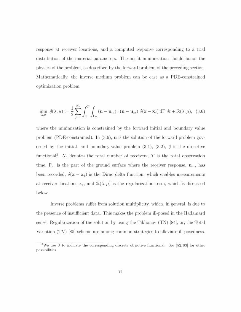
response at receiver locations, and a computed response corresponding to a trial
distribution of the material parameters. The misfit minimization should honor the
physics of the problem, as described by the forward problem of the preceding section.
Mathematically, the inverse medium problem can be cast as a PDE-constrained
optimization problem:
minλ,µ
J(λ, µ) :=1
2
Nr∑
j=1
∫ T
0
∫
Γm
(u− um) · (u− um) δ(x− xj) dΓ dt+ R(λ, µ), (3.6)
where the minimization is constrained by the forward initial and boundary value
problem (PDE-constrained). In (3.6), u is the solution of the forward problem gov-
erned by the initial- and boundary-value problem (3.1), (3.2), J is the objective
functional3, Nr denotes the total number of receivers, T is the total observation
time, Γm is the part of the ground surface where the receiver response, um, has
been recorded, δ(x − xj) is the Dirac delta function, which enables measurements
at receiver locations xj , and R(λ, µ) is the regularization term, which is discussed
below.
Inverse problems suffer from solution multiplicity, which, in general, is due to
the presence of insufficient data. This makes the problem ill-posed in the Hadamard
sense. Regularization of the solution by using the Tikhonov (TN) [84], or, the Total
Variation (TV) [85] scheme are among common strategies to alleviate ill-posedness.
3We use J to indicate the corresponding discrete objective functional. See [82, 83] for otherpossibilities.
71
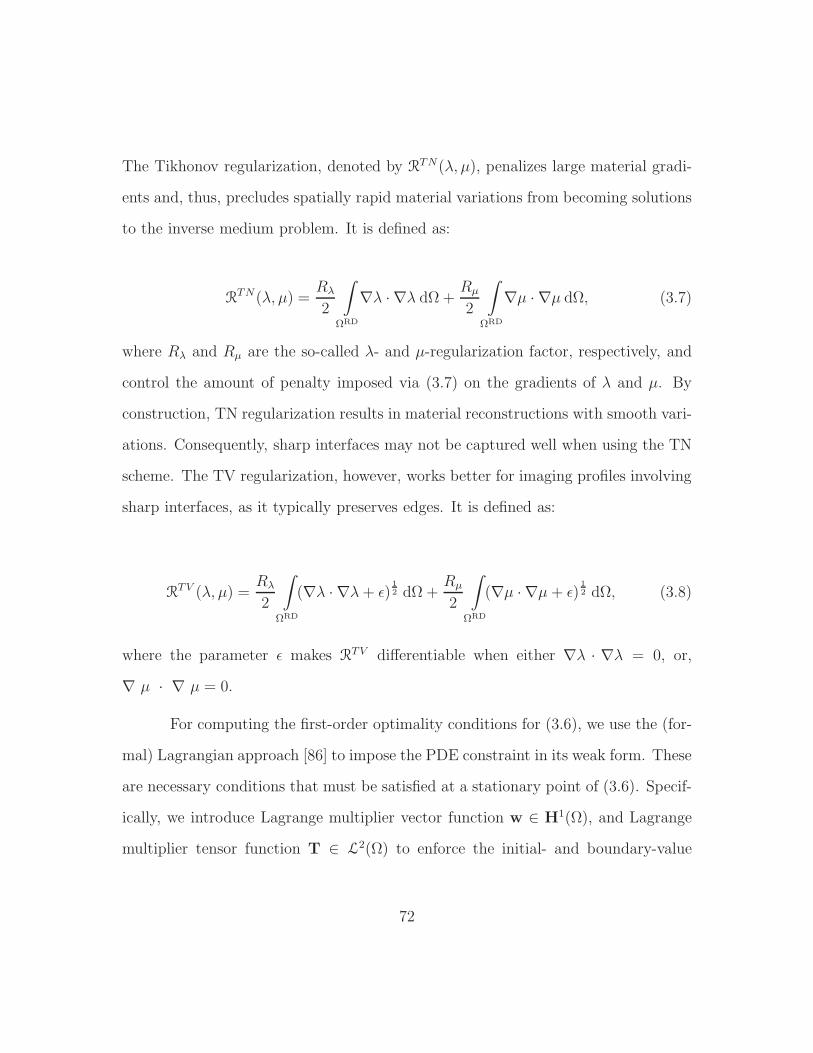
The Tikhonov regularization, denoted by RTN(λ, µ), penalizes large material gradi-
ents and, thus, precludes spatially rapid material variations from becoming solutions
to the inverse medium problem. It is defined as:
RTN(λ, µ) =
Rλ
2
∫
ΩRD
∇λ · ∇λ dΩ +Rµ
2
∫
ΩRD
∇µ · ∇µ dΩ, (3.7)
where Rλ and Rµ are the so-called λ- and µ-regularization factor, respectively, and
control the amount of penalty imposed via (3.7) on the gradients of λ and µ. By
construction, TN regularization results in material reconstructions with smooth vari-
ations. Consequently, sharp interfaces may not be captured well when using the TN
scheme. The TV regularization, however, works better for imaging profiles involving
sharp interfaces, as it typically preserves edges. It is defined as:
RTV (λ, µ) =Rλ
2
∫
ΩRD
(∇λ · ∇λ+ ǫ)1
2 dΩ +Rµ
2
∫
ΩRD
(∇µ · ∇µ+ ǫ)1
2 dΩ, (3.8)
where the parameter ǫ makes RTV differentiable when either ∇λ · ∇λ = 0, or,
∇ µ · ∇ µ = 0.
For computing the first-order optimality conditions for (3.6), we use the (for-
mal) Lagrangian approach [86] to impose the PDE constraint in its weak form. These
are necessary conditions that must be satisfied at a stationary point of (3.6). Specif-
ically, we introduce Lagrange multiplier vector function w ∈ H1(Ω), and Lagrange
multiplier tensor function T ∈ L2(Ω) to enforce the initial- and boundary-value
72
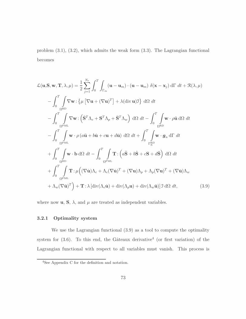
problem (3.1), (3.2), which admits the weak form (3.3). The Lagrangian functional
becomes
L(u,S,w,T, λ, µ) =1
2
Nr∑
j=1
∫ T
0
∫
Γm
(u− um) · (u− um) δ(x− xj) dΓ dt+ R(λ, µ)
−∫ T
0
∫
ΩRD
∇w :µ[∇u+ (∇u)T
]+ λ(divu)I
dΩ dt
−∫ T
0
∫
ΩPML
∇w :(STΛe + STΛp + STΛw
)dΩ dt−
∫ T
0
∫
ΩRD
w · ρu dΩ dt
−∫ T
0
∫
ΩPML
w · ρ (au+ bu+ cu+ du) dΩ dt+
∫ T
0
∫
ΓRD
N
w · gn dΓ dt
+
∫ T
0
∫
ΩRD
w · b dΩ dt−∫ T
0
∫
ΩPML
T :(aS+ bS+ cS+ dS
)dΩ dt
+
∫ T
0
∫
ΩPML
T :µ((∇u)Λe + Λe(∇u)T + (∇u)Λp + Λp(∇u)T + (∇u)Λw
+ Λw(∇u)T)+T :λ [div(Λeu) + div(Λpu) + div(Λwu)] I dΩ dt, (3.9)
where now u, S, λ, and µ are treated as independent variables.
3.2.1 Optimality system
We use the Lagrangian functional (3.9) as a tool to compute the optimality
system for (3.6). To this end, the Gateaux derivative4 (or first variation) of the
Lagrangian functional with respect to all variables must vanish. This process is
4See Appendix C for the definition and notation.
73

discussed next.
3.2.1.1 The state problem
Taking the derivatives of the Lagrangian functional L with respect to w and
T in directions w ∈ H1(Ω) and T ∈ L2(Ω), and setting it to zero, results in the state
problem, which is identical to (3.3). That is
L′(u,S,w,T, λ, µ)(w, T) = 0. (3.10)
3.2.1.2 The adjoint problem
We now take the derivative of L with respect to u and S in directions
u ∈ H1(Ω) and S ∈ L2(Ω). This yields
74
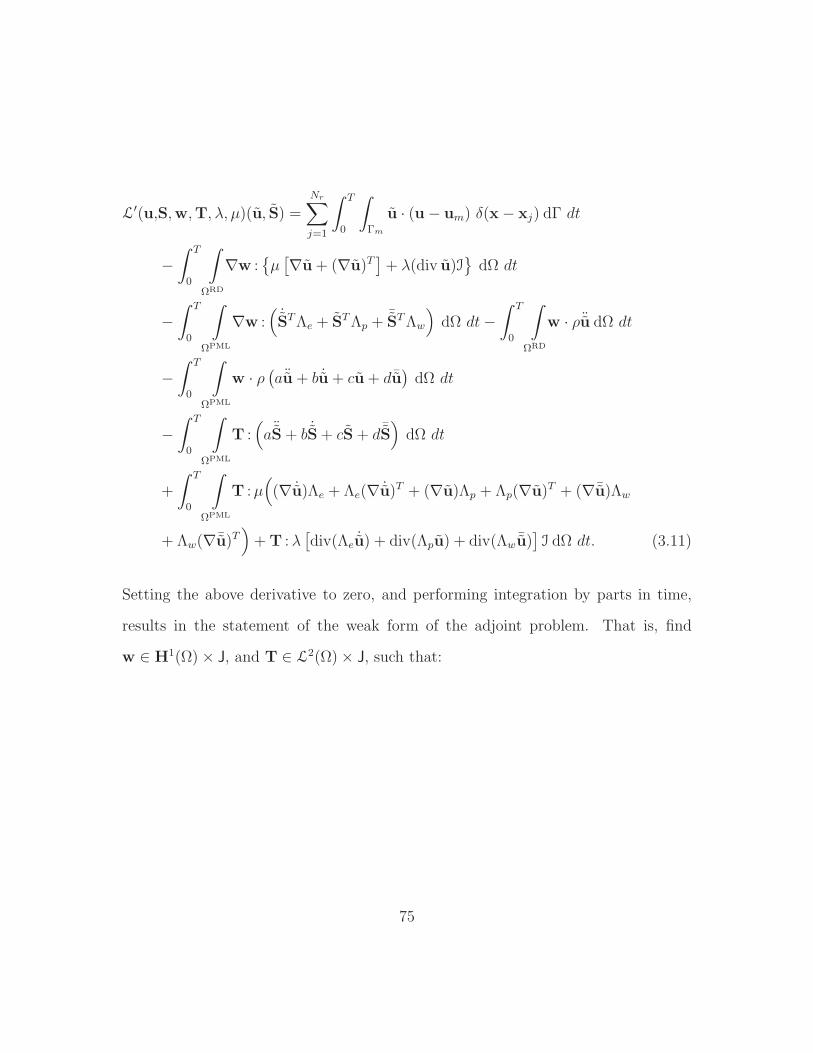
L′(u,S,w,T, λ, µ)(u, S) =Nr∑
j=1
∫ T
0
∫
Γm
u · (u− um) δ(x− xj) dΓ dt
−∫ T
0
∫
ΩRD
∇w :µ[∇u+ (∇u)T
]+ λ(div u)I
dΩ dt
−∫ T
0
∫
ΩPML
∇w :(˙STΛe + STΛp +
¯STΛw
)dΩ dt−
∫ T
0
∫
ΩRD
w · ρ¨u dΩ dt
−∫ T
0
∫
ΩPML
w · ρ(a¨u+ b ˙u+ cu+ d ¯u
)dΩ dt
−∫ T
0
∫
ΩPML
T :(a¨S+ b ˙S+ cS+ d ¯S
)dΩ dt
+
∫ T
0
∫
ΩPML
T :µ((∇ ˙u)Λe + Λe(∇ ˙u)T + (∇u)Λp + Λp(∇u)T + (∇¯u)Λw
+ Λw(∇¯u)T)+T :λ
[div(Λe
˙u) + div(Λpu) + div(Λw¯u)]I dΩ dt. (3.11)
Setting the above derivative to zero, and performing integration by parts in time,
results in the statement of the weak form of the adjoint problem. That is, find
w ∈ H1(Ω)× J, and T ∈ L2(Ω)× J, such that:
75
∫
ΩRD
∇u :µ[∇w + (∇w)T
]+ λ(divw)I
dΩ+
+
∫
ΩRD
u · ρw dΩ +
∫
ΩPML
u · ρ (aw − bw + cw− dw) dΩ
−∫
ΩPML
∇u :µ[−TΛe − TTΛe +TΛp +TTΛp − TΛw − TTΛw
]
+ λ[−T : div(Λeu) +T : div(Λpu)− T : div(Λwu)
]I dΩ
=
Nr∑
j=1
∫
Γm
u · (u− um) δ(x− xj) dΓ, (3.12a)
∫
ΩPML
∇w : STΛe −∇w : STΛp +∇w : STΛw dΩ =
∫
ΩPML
S :(aT− bT + cS− dT
)dΩ
(3.12b)
for every u ∈ H1(Ω) and S ∈ L2(Ω), where w(x, T ) = 0, and T(x, T ) = 0.
We remark that the adjoint problem (3.12) is a final-value problem and, thus,
is solved backwards in time5; it is driven by the misfit between a computed response,
and the measured response at receiver locations. Moreover, the operators implicated
in the adjoint problem are very similar to those of the state problem: they involve
transposition of the system matrices, and sign reversal for terms involving history,
and first-order time derivatives. In this regard, we obtain the following semi-discrete
form for the adjoint problem:
5See [87] for other possibilities, and [88–90] for alternative approaches.
76
Mdadj −CT dadj +KTdadj −GT dadj = fadj, (3.13a)
dadj =
∫ t
0
dadj(τ)|PML dτ, (3.13b)
where superscript “adj” refers to the adjoint problem, dadj = (wTh ,T
Th )
T is the vector
of nodal unknowns comprising discrete values of w in ΩRD∪ΩPML and discrete values
of T only in ΩPML, and fadj is a vector comprising the misfit at receiver locations.
Moreover, system matricesM, C, K, G, are identical to those of the forward problem
and, thus, with minor adjustments, an implementation of the forward problem can
also be used for the solution of the adjoint problem.
The matrixM in (3.13) can be diagonalized by using spectral elements, similar
to what we did in (3.5). We rewrite (3.13) as a first-order system
d
dt
y0
y1
My2
=
0 I 00 0 IGT −KT CT
y0
y1
y2
+
00fadj
, (3.14)
where y0 = dadj, y1 = dadj, y2 = dadj, with final values y0(T ) = 0, y1(T ) = 0, and
y2(T ) = 0. We use an explicit RK-4 method to integrate (3.14) in time. The scheme
is outlined in Appendix B.3.
3.2.1.3 The control problems
Lastly, we take the derivative of L with respect to λ and µ in directions λ
and µ, which yields the reduced gradients with respect to λ and µ, respectively. We
77
restrict the reduced gradients to ΩRD (the material properties at the interfaces ΓI
are extended into the PML buffer). For the TN regularization, this yields
L′(u,S,w,T, λ, µ)(λ) = Rλ
∫
ΩRD
∇λ · ∇λ dΩ−∫ T
0
∫
ΩRD
λ ∇w :(divu)I dΩ dt, (3.15a)
L′(u,S,w,T, λ, µ)(µ) = Rµ
∫
ΩRD
∇µ · ∇µ dΩ−∫ T
0
∫
ΩRD
µ ∇u :[∇w + (∇w)T
]dΩ dt.
(3.15b)
Setting the above derivatives to zero, results in the control problems. Similarly, for
the TV regularization, the control problems read
L′(u,S,w,T, λ, µ)(λ) = Rλ
∫
ΩRD
∇λ · ∇λ(∇λ · ∇λ+ ǫ)
1
2
dΩ−∫ T
0
∫
ΩRD
λ ∇w :(divu)I dΩ dt,
(3.16a)
L′(u,S,w,T, λ, µ)(µ) = Rµ
∫
ΩRD
∇µ · ∇µ(∇µ · ∇µ+ ǫ)
1
2
dΩ
−∫ T
0
∫
ΩRD
µ ∇u :[∇w + (∇w)T
]dΩ dt. (3.16b)
Discretization of either (3.15) or (3.16) result in the following form
Mgλ = Rλ gλreg + gλ
mis, (3.17a)
Mgµ = Rµ gµreg + gµ
mis, (3.17b)
78
where M is a mass-like matrix, gλ and gµ is the vector of discrete values of the
(reduced) gradient for λ and µ, respectively, and gλreg, g
µreg and gλ
mis, gµmis are the
associated vectors corresponding to the regularization-part and misfit-part of gλ and
gµ. We refer to Appendix A.4 for matrix and vector definitions, and discretization
details.
3.2.2 The inversion process
A solution of (3.6) requires simultaneous satisfaction of the state problem
(3.5), the adjoint problem (3.14), and the control problems (3.17). This approach
–a full-space method– is, in principle, possible [91]; however, the associated com-
putational cost can be substantial. Alternatively, a reduced-space method may
be adopted, in which, discrete material properties are updated iteratively, using
a gradient-based minimization scheme. The latter approach is employed here, and is
discussed next.
We start with an assumed initial spatial distribution of the control parameters
(λ and µ), and solve the state problem (3.5) to obtain dst = (uTh ,S
Th )
T . With the
misfit known, we solve the adjoint problem (3.14) and obtain dadj = (wTh ,T
Th )
T . With
uh and wh known, the (reduced) material gradients gλ and gµ, can be computed from
(3.17). Thus, the vector of material values, at iteration k + 1, can be computed by
using a search direction via
79
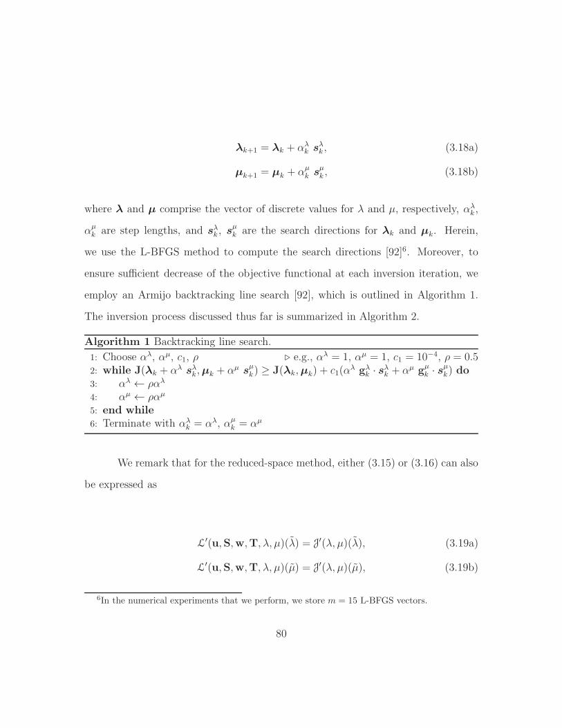
λk+1 = λk + αλk sλk , (3.18a)
µk+1 = µk + αµk s
µk , (3.18b)
where λ and µ comprise the vector of discrete values for λ and µ, respectively, αλk ,
αµk are step lengths, and sλk , s
µk are the search directions for λk and µk. Herein,
we use the L-BFGS method to compute the search directions [92]6. Moreover, to
ensure sufficient decrease of the objective functional at each inversion iteration, we
employ an Armijo backtracking line search [92], which is outlined in Algorithm 1.
The inversion process discussed thus far is summarized in Algorithm 2.
Algorithm 1 Backtracking line search.
1: Choose αλ, αµ, c1, ρ ⊲ e.g., αλ = 1, αµ = 1, c1 = 10−4, ρ = 0.52: while J(λk + αλ sλk ,µk + αµ s
µk) ≥ J(λk,µk) + c1(α
λ gλk · sλk + αµ gµ
k · sµk) do
3: αλ ← ραλ
4: αµ ← ραµ
5: end while6: Terminate with αλ
k = αλ, αµk = αµ
We remark that for the reduced-space method, either (3.15) or (3.16) can also
be expressed as
L′(u,S,w,T, λ, µ)(λ) = J′(λ, µ)(λ), (3.19a)
L′(u,S,w,T, λ, µ)(µ) = J′(λ, µ)(µ), (3.19b)
6In the numerical experiments that we perform, we store m = 15 L-BFGS vectors.
80
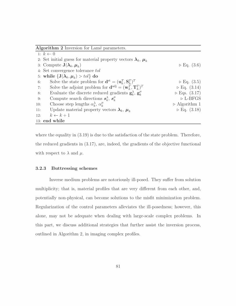
Algorithm 2 Inversion for Lame parameters.
1: k ← 02: Set initial guess for material property vectors λk, µk
3: Compute J(λk,µk) ⊲ Eq. (3.6)4: Set convergence tolerance tol5: while J(λk,µk) > tol do6: Solve the state problem for dst = (uT
h ,STh )
T ⊲ Eq. (3.5)7: Solve the adjoint problem for dadj = (wT
h ,TTh )
T ⊲ Eq. (3.14)8: Evaluate the discrete reduced gradients gλ
k , gµk ⊲ Eqs. (3.17)
9: Compute search directions sλk , sµk ⊲ L-BFGS
10: Choose step lengths αλk , α
µk ⊲ Algorithm 1
11: Update material property vectors λk, µk ⊲ Eq. (3.18)12: k ← k + 113: end while
where the equality in (3.19) is due to the satisfaction of the state problem. Therefore,
the reduced gradients in (3.17), are, indeed, the gradients of the objective functional
with respect to λ and µ.
3.2.3 Buttressing schemes
Inverse medium problems are notoriously ill-posed. They suffer from solution
multiplicity; that is, material profiles that are very different from each other, and,
potentially non-physical, can become solutions to the misfit minimization problem.
Regularization of the control parameters alleviates the ill-posedness; however, this
alone, may not be adequate when dealing with large-scale complex problems. In
this part, we discuss additional strategies that further assist the inversion process,
outlined in Algorithm 2, in imaging complex profiles.
81

3.2.3.1 Regularization factor selection and continuation
Computation of the (reduced) gradients (3.17) necessitates selection of the
regularization factors Rλ and Rµ. A common strategy is to use Morozov’s discrepancy
principle [93], where a constant value for the regularization factor is used throughout
the inversion process. Here, we discuss a simple and practical approach that was
initially developed for acoustic inversion [56], and, later, was successfully applied to
problems involving elastic inversion [57].
We start by rewriting the discrete control problem (3.17), either for λ or µ,
in the following generic form
Mg = R greg + gmis, (3.20)
where g refers to the vector of discrete values of the (reduced) gradient, either for λ
or µ, greg and gmis are the associated vectors corresponding to the regularization-part
and misfit-part of g, and R is the regularization factor yet to be determined. The
main idea is that the “size” of R greg should be proportional to that of gmis at each
inversion iteration. We define the following unit vectors for the two components of
the gradient vector
nreg =greg
‖greg‖, nmis =
gmis
‖gmis‖, (3.21)
where ‖ · ‖ denotes the Euclidean norm. Equation (3.20) can then be written as
82
Mg = R ‖greg‖ nreg + ‖gmis‖ nmis (3.22a)
= ‖gmis‖(R‖greg‖‖gmis‖
nreg + nmis
)
= ‖gmis‖(℘ nreg + nmis
), (3.22b)
where,
℘ = R‖greg‖‖gmis‖
. (3.22c)
In (3.22b), for the “size” of ℘ nreg to be proportional to nmis throughout the entire
inversion process, one may choose 0 < ℘ ≤ 1. Once a value for ℘ has been decided,
R can be computed via
R = ℘‖gmis‖‖greg‖
, (3.23)
where ℘ can take large values (e.g., 0.5) at early stages of the inversion process
and, thus, narrow down the initial search space. As the inversion evolves, ℘ can be
continuously reduced (e.g., down to 0.3) to allow for profile refinement.
3.2.3.2 Source-frequency continuation
Using loading sources with low-frequency content result in an overall image
of the medium that lacks fine features. To allow for more details, and fine-tune
the profile, one needs to probe with higher frequency content. Thus, the inversion
process can be initiated with a signal having a low-frequency content and, then,
83
the frequency range can be increased progressively as inversion evolves. This can be
achieved by using a set of probing signals, ordered such that each signal has a broader
range of frequencies than the previous ones. The inversion process then begins with
using the first signal. Upon convergence, the profile is used as a starting point for
the second signal, and the process is repeated for all signals.
3.2.3.3 Biased search direction for λ
Simultaneous inversion for both λ and µ is remarkably challenging [61]. As
we demonstrate in Section 3.3.2, the objective functional (3.6) is more sensitive to
µ, than to λ. Consequently, as the inversion evolves, the µ-profile converges faster
than that of λ. In [57], a biasing scheme was proposed to accelerate the convergence
of the λ-profile, such that, at the early stages of inversion, the search direction for λ
is biased according to that of µ.
The main idea is that due to physical considerations, the λ-profile should be,
more or less, similar to the µ-profile. Hence, during the early inversion iterations,
the search direction for λ is biased according to
sλk ← ‖sλk‖(W
sµk
‖sµk‖+ (1−W )
sλk‖sλk‖
), (3.24)
where W is a weight that imposes the biasing amount. We assign full weight (W = 1)
on µ at the first inversion iteration, and reduce it linearly down to zero as iterates
evolve (say at k = 50). After that, we let λ evolve on its own, according to the
original, unbiased search direction.
84
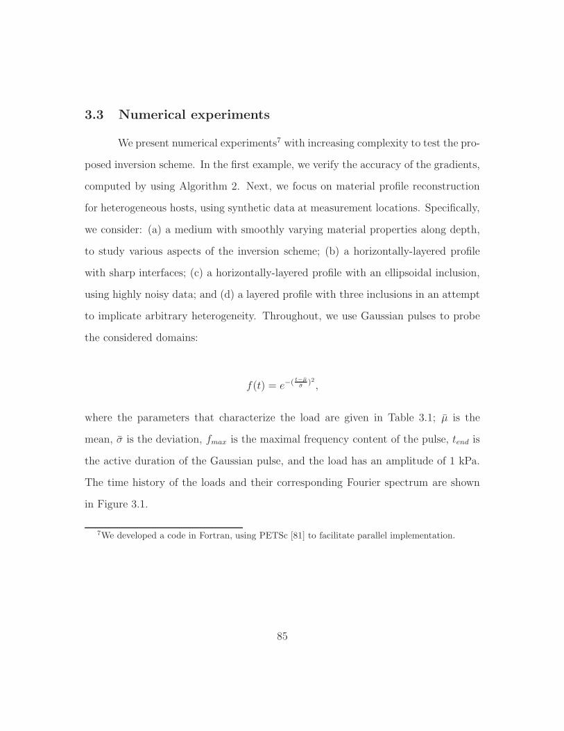
3.3 Numerical experiments
We present numerical experiments7 with increasing complexity to test the pro-
posed inversion scheme. In the first example, we verify the accuracy of the gradients,
computed by using Algorithm 2. Next, we focus on material profile reconstruction
for heterogeneous hosts, using synthetic data at measurement locations. Specifically,
we consider: (a) a medium with smoothly varying material properties along depth,
to study various aspects of the inversion scheme; (b) a horizontally-layered profile
with sharp interfaces; (c) a horizontally-layered profile with an ellipsoidal inclusion,
using highly noisy data; and (d) a layered profile with three inclusions in an attempt
to implicate arbitrary heterogeneity. Throughout, we use Gaussian pulses to probe
the considered domains:
f(t) = e−( t−µ
σ)2 ,
where the parameters that characterize the load are given in Table 3.1; µ is the
mean, σ is the deviation, fmax is the maximal frequency content of the pulse, tend is
the active duration of the Gaussian pulse, and the load has an amplitude of 1 kPa.
The time history of the loads and their corresponding Fourier spectrum are shown
in Figure 3.1.
7We developed a code in Fortran, using PETSc [81] to facilitate parallel implementation.
85
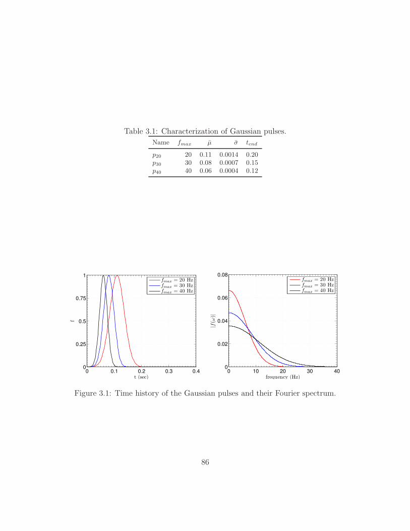
Table 3.1: Characterization of Gaussian pulses.
Name fmax µ σ tend
p20 20 0.11 0.0014 0.20p30 30 0.08 0.0007 0.15p40 40 0.06 0.0004 0.12
0 0.1 0.2 0.3 0.40
0.25
0.5
0.75
1
t (sec)
f
fmax = 20 Hzfmax = 30 Hzfmax = 40 Hz
0 10 20 30 400
0.02
0.04
0.06
0.08
frequency (Hz)
|f(ω
)|
fmax = 20 Hzfmax = 30 Hzfmax = 40 Hz
Figure 3.1: Time history of the Gaussian pulses and their Fourier spectrum.
86
3.3.1 Numerical verification of the material gradients
Accurate computation of the discrete gradients is crucial for the robustness
of Algorithm 2. The gradients of the objective functional with respect to the control
parameters can be computed either by the optimize-then-discretize, or, the discretize-
then-optimize approach [68]. While the discretize-then-optimize method yields the
exact discrete gradients of the discrete objective functional [94], this is not always
the case with the optimize-then-discretize scheme [95].
In this part, through a numerical experiment, we demonstrate that the dis-
crete gradients that we compute via the optimize-then-discretize technique, are accu-
rate, and equal to the discrete gradients of the discrete objective functional. To this
end, we consider a heterogeneous half-space with a smoothly varying material profile
along depth, given in (3.27), and mass density ρ = 2000 kg/m3, which, after trunca-
tion, is reduced to a cubic computational domain of length and width 24 m × 24 m,
and 45 m depth. A 5 m-thick PML is placed at the truncation boundaries, as
shown in Fig. 3.2. The material properties at the interfaces ΓI are extended into
the PML. The interior and PML domains are discretized by quadratic hexahedral
spectral elements of size 1 m (i.e., 27-noded bricks, and quadratic-quadratic pairs of
approximation for displacement and stress components in the PML, and, quadratic
approximations for the material properties), and ∆t = 9 × 10⁻⁴ s. Throughout, for
the PML parameters, we choose αo = 5, βo = 400 s 1, and a quadratic profile for
the attenuation functions, i.e., m = 2. To probe the medium, we consider vertical
stress loads with Gaussian pulse temporal signatures (see Table 3.1), applied on the
surface of the domain over a region (−11 m ≤ x, y ≤ 11 m), whereas receivers that
87
collect displacement response um(x, t) are also located in the same region, at every
grid point. To obtain synthetic data at the receiver locations, we use a model with
identical characteristics and dimensions as detailed above, but, with a refined dis-
cretization; i.e., element size of 0.5 m, and ∆t = 4.5× 10⁻⁴ s. The total duration of
the simulation is T = 0.5 s. We compare directional finite differences of the discrete
objective functional, with directional gradients obtained from (3.17). We start by
defining the finite difference directional derivatives
dfdh (λ,µ)(λ) :=J(λ+ hλ,µ)− J(λ,µ)
h, (3.25a)
dfdh (λ,µ)(µ) :=J(λ,µ+ hµ)− J(λ,µ)
h, (3.25b)
where λ and µ is the discrete direction vector for λ and µ, respectively. The direc-
tional derivatives obtained via the control problems (3.17) are
dco(λ,µ)(λ) = λ M gλ, (3.26a)
dco(λ,µ)(µ) = µ M gµ. (3.26b)
Next, we verify that (3.25) and (3.26) produce identical values for several
choices that we make for λ and µ, with regularization factors8 Rλ = Rµ = 0. We
consider perturbations λ or µ: the unit vector is zero everywhere except at the
8Zero values are considered since convergence difficulties that may arise stem from the misfitpart of the objective functional, and not from the regularization part. Nevertheless, we have alsosuccessfully verified the accuracy of the regularization component of the gradients.
88
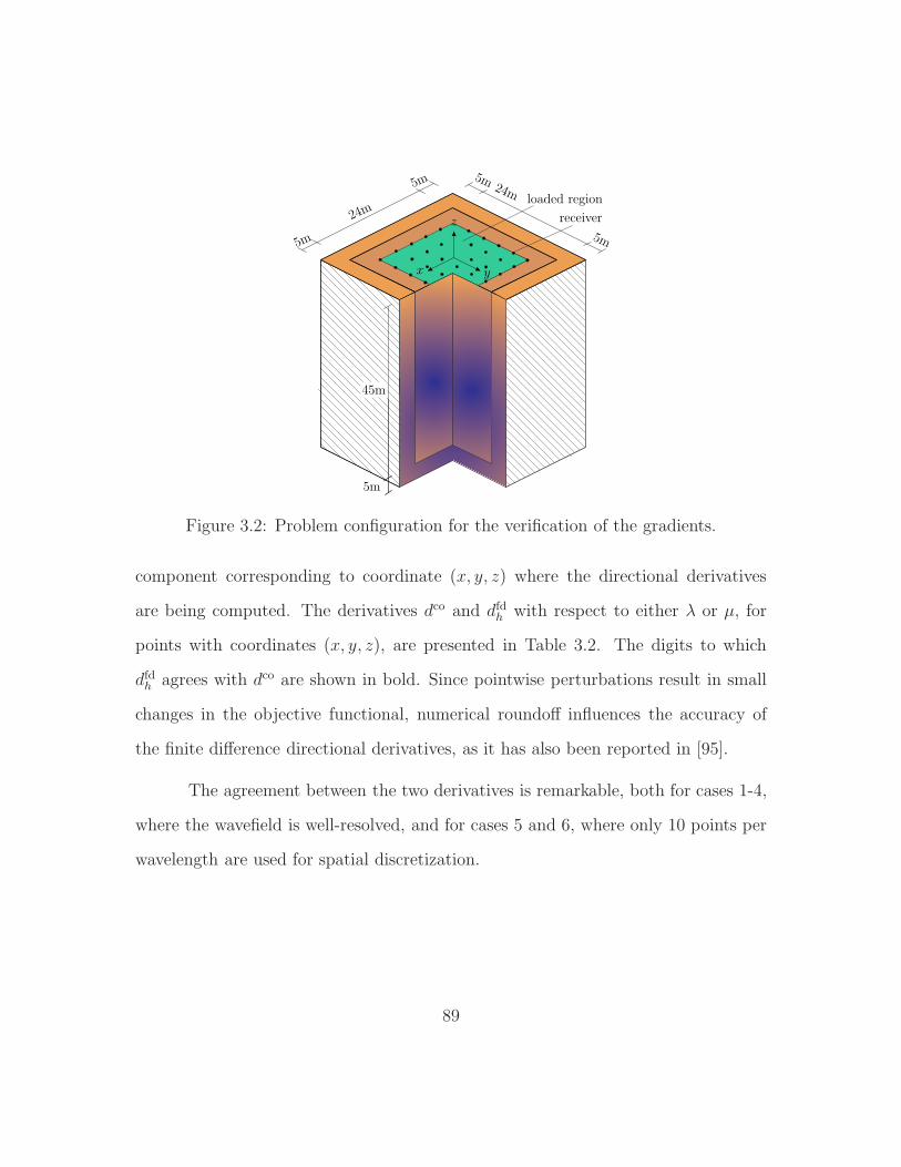
x y
z
Figure 3.2: Problem configuration for the verification of the gradients.
component corresponding to coordinate (x, y, z) where the directional derivatives
are being computed. The derivatives dco and dfdh with respect to either λ or µ, for
points with coordinates (x, y, z), are presented in Table 3.2. The digits to which
dfdh agrees with dco are shown in bold. Since pointwise perturbations result in small
changes in the objective functional, numerical roundoff influences the accuracy of
the finite difference directional derivatives, as it has also been reported in [95].
The agreement between the two derivatives is remarkable, both for cases 1-4,
where the wavefield is well-resolved, and for cases 5 and 6, where only 10 points per
wavelength are used for spatial discretization.
89
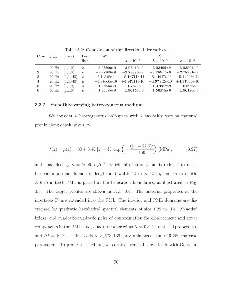
Table 3.2: Comparison of the directional derivatives.
Case fmax (x,y,z) Pert. dco dfdhfield h = 10−3 h = 10−4 h = 10−5
1 20 Hz (1,1,0) λ −3.03500e-9 −3.03416e-9 −3.03496e-9 −3.03501e-92 20 Hz (1,1,0) µ −2.78908e-9 −2.78875e-9 −2.78917e-9 −2.78921e-93 20 Hz (1,1,-40) λ −5.14848e-11 −5.14711e-11 −5.14647e-11 −5.14996e-114 20 Hz (1,1,-40) µ +4.97666e-10 +4.97411e-10 +4.97512e-10 +4.97366e-105 40 Hz (1,1,0) λ −1.07645e-9 −1.07623e-9 −1.07652e-9 −1.07656e-96 40 Hz (1,1,0) µ −1.56155e-9 −1.56153e-9 −1.56178e-9 −1.56180e-9
3.3.2 Smoothly varying heterogeneous medium
We consider a heterogeneous half-space with a smoothly varying material
profile along depth, given by
λ(z) = µ(z) = 80 + 0.45 |z|+ 35 exp(− (|z| − 22.5)2
150
)(MPa), (3.27)
and mass density ρ = 2000 kg/m3, which, after truncation, is reduced to a cu-
bic computational domain of length and width 40 m × 40 m, and 45 m depth.
A 6.25 m-thick PML is placed at the truncation boundaries, as illustrated in Fig.
3.3. The target profiles are shown in Fig. 3.4. The material properties at the
interfaces ΓI are extended into the PML. The interior and PML domains are dis-
cretized by quadratic hexahedral spectral elements of size 1.25 m (i.e., 27-noded
bricks, and quadratic-quadratic pairs of approximation for displacement and stress
components in the PML, and, quadratic approximations for the material properties),
and ∆t = 10−3 s. This leads to 3, 578, 136 state unknowns, and 616, 850 material
parameters. To probe the medium, we consider vertical stress loads with Gaussian
90
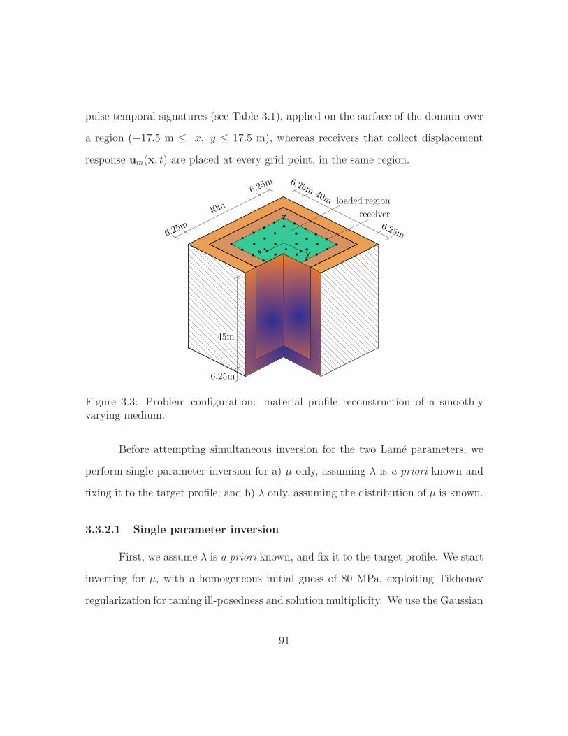
pulse temporal signatures (see Table 3.1), applied on the surface of the domain over
a region (−17.5 m ≤ x, y ≤ 17.5 m), whereas receivers that collect displacement
response um(x, t) are placed at every grid point, in the same region.
x y
z
Figure 3.3: Problem configuration: material profile reconstruction of a smoothlyvarying medium.
Before attempting simultaneous inversion for the two Lame parameters, we
perform single parameter inversion for a) µ only, assuming λ is a priori known and
fixing it to the target profile; and b) λ only, assuming the distribution of µ is known.
3.3.2.1 Single parameter inversion
First, we assume λ is a priori known, and fix it to the target profile. We start
inverting for µ, with a homogeneous initial guess of 80 MPa, exploiting Tikhonov
regularization for taming ill-posedness and solution multiplicity. We use the Gaussian
91
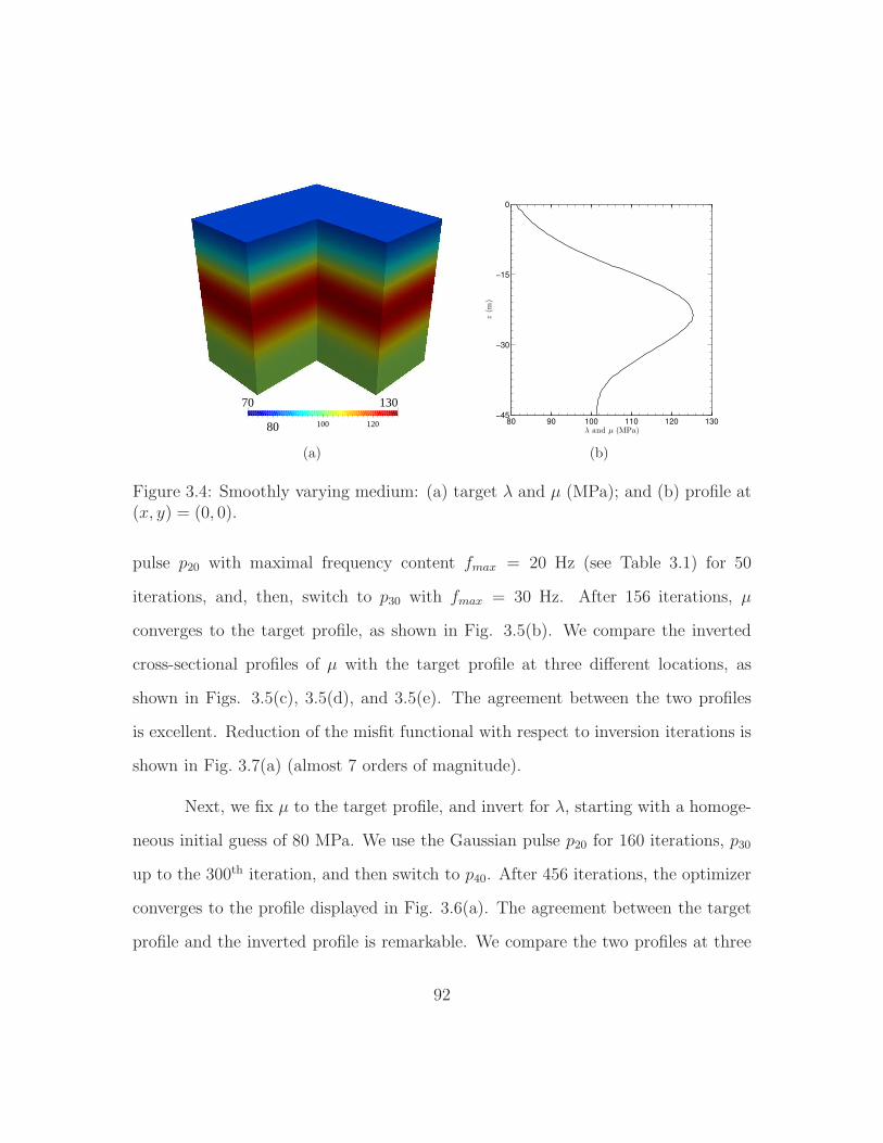
80 100 120
70 130
(a)
80 90 100 110 120 130−45
−30
−15
0
z(m
)
λ and µ (MPa)
(b)
Figure 3.4: Smoothly varying medium: (a) target λ and µ (MPa); and (b) profile at(x, y) = (0, 0).
pulse p20 with maximal frequency content fmax = 20 Hz (see Table 3.1) for 50
iterations, and, then, switch to p30 with fmax = 30 Hz. After 156 iterations, µ
converges to the target profile, as shown in Fig. 3.5(b). We compare the inverted
cross-sectional profiles of µ with the target profile at three different locations, as
shown in Figs. 3.5(c), 3.5(d), and 3.5(e). The agreement between the two profiles
is excellent. Reduction of the misfit functional with respect to inversion iterations is
shown in Fig. 3.7(a) (almost 7 orders of magnitude).
Next, we fix µ to the target profile, and invert for λ, starting with a homoge-
neous initial guess of 80 MPa. We use the Gaussian pulse p20 for 160 iterations, p30
up to the 300th iteration, and then switch to p40. After 456 iterations, the optimizer
converges to the profile displayed in Fig. 3.6(a). The agreement between the target
profile and the inverted profile is remarkable. We compare the two profiles at three
92
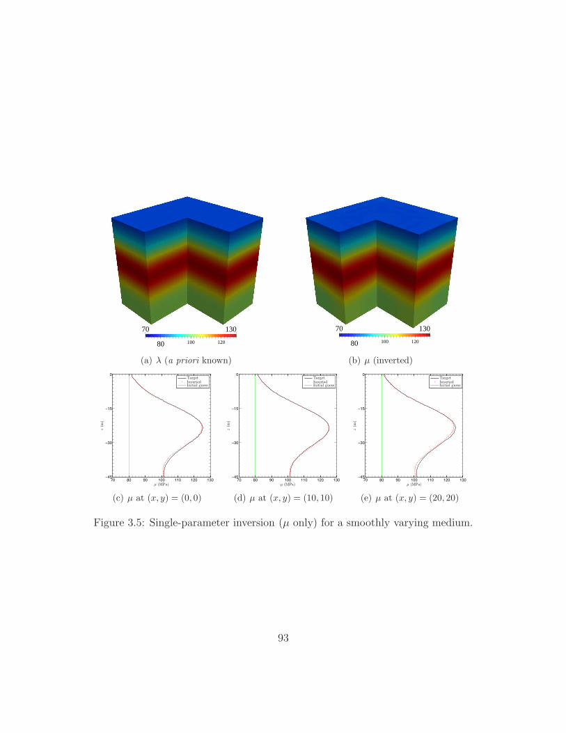
80 100 120
70 130
(a) λ (a priori known)
80 100 120
70 130
(b) µ (inverted)
70 80 90 100 110 120 130−45
−30
−15
0
µ (MPa)
z(m
)
TargetInvertedInitial guess
(c) µ at (x, y) = (0, 0)
70 80 90 100 110 120 130−45
−30
−15
0
µ (MPa)
z(m
)
TargetInvertedInitial guess
(d) µ at (x, y) = (10, 10)
70 80 90 100 110 120 130−45
−30
−15
0
µ (MPa)
z(m
)
TargetInvertedInitial guess
(e) µ at (x, y) = (20, 20)
Figure 3.5: Single-parameter inversion (µ only) for a smoothly varying medium.
93
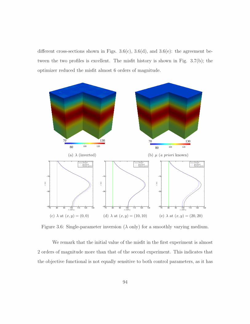
different cross-sections shown in Figs. 3.6(c), 3.6(d), and 3.6(e): the agreement be-
tween the two profiles is excellent. The misfit history is shown in Fig. 3.7(b); the
optimizer reduced the misfit almost 6 orders of magnitude.
80 100 120
70 130
(a) λ (inverted)
80 100 120
70 130
(b) µ (a priori known)
70 80 90 100 110 120 130−45
−30
−15
0
z(m
)
λ (MPa)
TargetInvertedInitial guess
(c) λ at (x, y) = (0, 0)
70 80 90 100 110 120 130−45
−30
−15
0
z(m
)
λ (MPa)
TargetInvertedInitial guess
(d) λ at (x, y) = (10, 10)
70 80 90 100 110 120 130−45
−30
−15
0
z(m
)
λ (MPa)
TargetInvertedInitial guess
(e) λ at (x, y) = (20, 20)
Figure 3.6: Single-parameter inversion (λ only) for a smoothly varying medium.
We remark that the initial value of the misfit in the first experiment is almost
2 orders of magnitude more than that of the second experiment. This indicates that
the objective functional is not equally sensitive to both control parameters, as it has
94
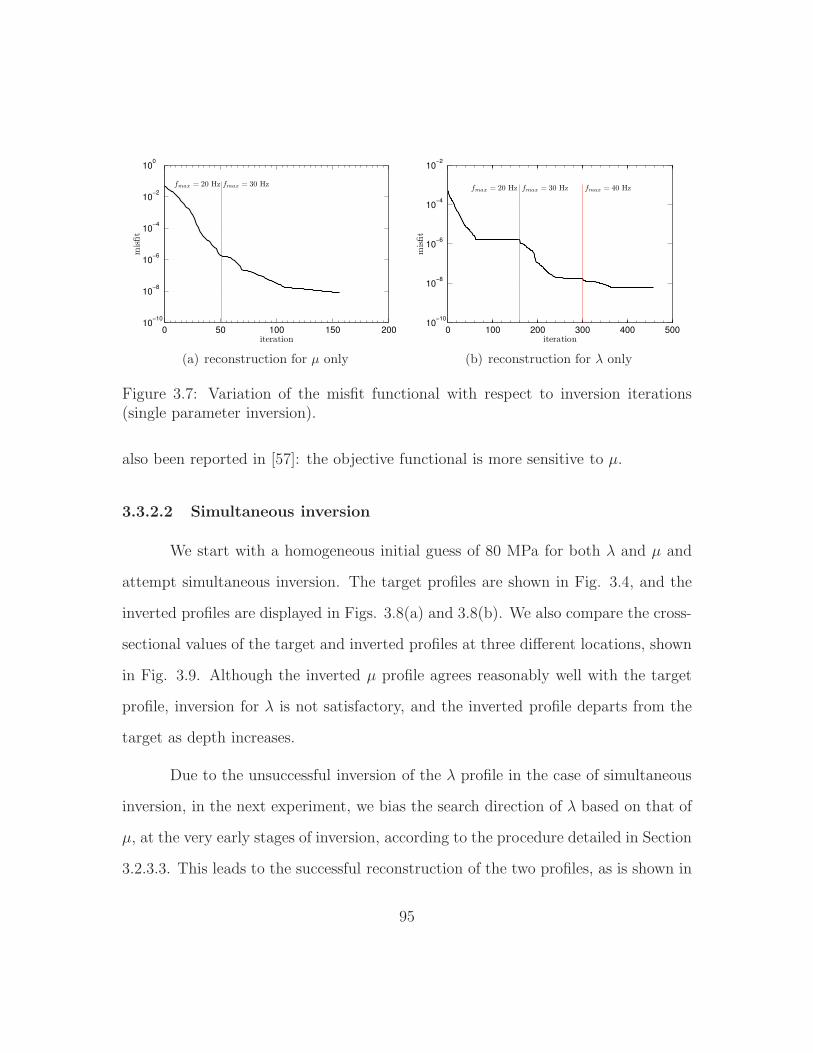
0 50 100 150 20010
−10
10−8
10−6
10−4
10−2
100
iteration
misfit
fmax = 20 Hz fmax = 30 Hz
(a) reconstruction for µ only
0 100 200 300 400 50010
−10
10−8
10−6
10−4
10−2
iteration
misfit
fmax = 20 Hz fmax = 30 Hz fmax = 40 Hz
(b) reconstruction for λ only
Figure 3.7: Variation of the misfit functional with respect to inversion iterations(single parameter inversion).
also been reported in [57]: the objective functional is more sensitive to µ.
3.3.2.2 Simultaneous inversion
We start with a homogeneous initial guess of 80 MPa for both λ and µ and
attempt simultaneous inversion. The target profiles are shown in Fig. 3.4, and the
inverted profiles are displayed in Figs. 3.8(a) and 3.8(b). We also compare the cross-
sectional values of the target and inverted profiles at three different locations, shown
in Fig. 3.9. Although the inverted µ profile agrees reasonably well with the target
profile, inversion for λ is not satisfactory, and the inverted profile departs from the
target as depth increases.
Due to the unsuccessful inversion of the λ profile in the case of simultaneous
inversion, in the next experiment, we bias the search direction of λ based on that of
µ, at the very early stages of inversion, according to the procedure detailed in Section
3.2.3.3. This leads to the successful reconstruction of the two profiles, as is shown in
95
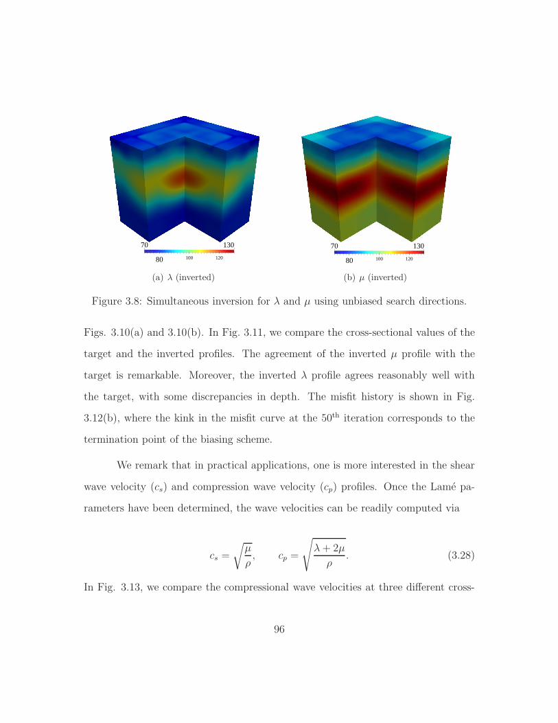
80 100 120
70 130
(a) λ (inverted)
80 100 120
70 130
(b) µ (inverted)
Figure 3.8: Simultaneous inversion for λ and µ using unbiased search directions.
Figs. 3.10(a) and 3.10(b). In Fig. 3.11, we compare the cross-sectional values of the
target and the inverted profiles. The agreement of the inverted µ profile with the
target is remarkable. Moreover, the inverted λ profile agrees reasonably well with
the target, with some discrepancies in depth. The misfit history is shown in Fig.
3.12(b), where the kink in the misfit curve at the 50th iteration corresponds to the
termination point of the biasing scheme.
We remark that in practical applications, one is more interested in the shear
wave velocity (cs) and compression wave velocity (cp) profiles. Once the Lame pa-
rameters have been determined, the wave velocities can be readily computed via
cs =
õ
ρ, cp =
√λ+ 2µ
ρ. (3.28)
In Fig. 3.13, we compare the compressional wave velocities at three different cross-
96
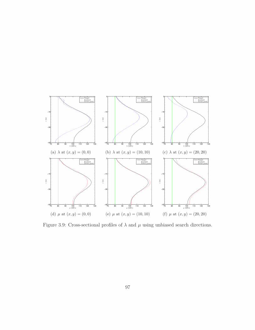
70 80 90 100 110 120 130−45
−30
−15
0
z(m
)
λ (MPa)
TargetInvertedInitial guess
(a) λ at (x, y) = (0, 0)
70 80 90 100 110 120 130−45
−30
−15
0
z(m
)
λ (MPa)
TargetInvertedInitial guess
(b) λ at (x, y) = (10, 10)
70 80 90 100 110 120 130−45
−30
−15
0
z(m
)
λ (MPa)
TargetInvertedInitial guess
(c) λ at (x, y) = (20, 20)
70 80 90 100 110 120 130−45
−30
−15
0
z(m
)
µ (MPa)
TargetInvertedInitial guess
(d) µ at (x, y) = (0, 0)
70 80 90 100 110 120 130−45
−30
−15
0
z(m
)
µ (MPa)
TargetInvertedInitial guess
(e) µ at (x, y) = (10, 10)
70 80 90 100 110 120 130−45
−30
−15
0z
(m)
µ (MPa)
TargetInvertedInitial guess
(f) µ at (x, y) = (20, 20)
Figure 3.9: Cross-sectional profiles of λ and µ using unbiased search directions.
97
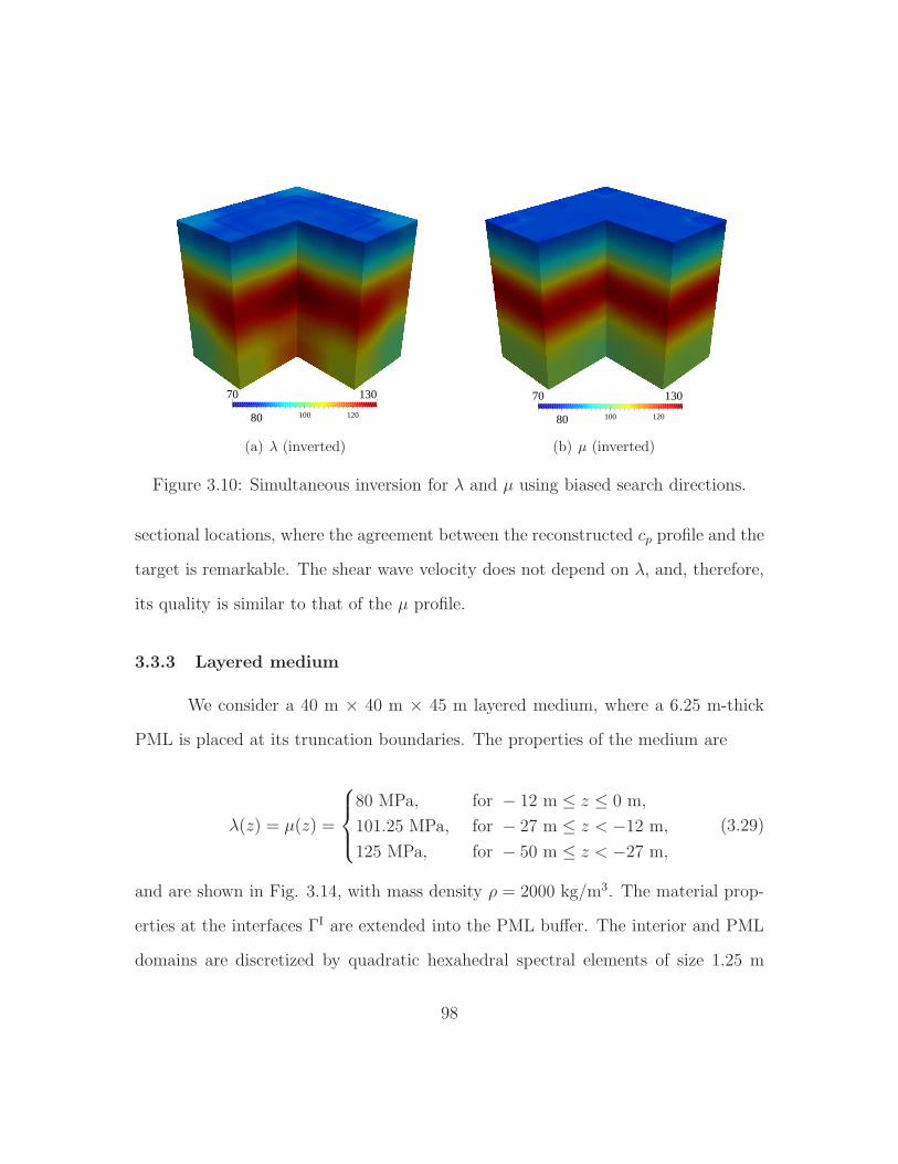
80 100 120
70 130
(a) λ (inverted)
80 100 120
70 130
(b) µ (inverted)
Figure 3.10: Simultaneous inversion for λ and µ using biased search directions.
sectional locations, where the agreement between the reconstructed cp profile and the
target is remarkable. The shear wave velocity does not depend on λ, and, therefore,
its quality is similar to that of the µ profile.
3.3.3 Layered medium
We consider a 40 m × 40 m × 45 m layered medium, where a 6.25 m-thick
PML is placed at its truncation boundaries. The properties of the medium are
λ(z) = µ(z) =
80 MPa, for − 12 m ≤ z ≤ 0 m,
101.25 MPa, for − 27 m ≤ z < −12 m,
125 MPa, for − 50 m ≤ z < −27 m,
(3.29)
and are shown in Fig. 3.14, with mass density ρ = 2000 kg/m3. The material prop-
erties at the interfaces ΓI are extended into the PML buffer. The interior and PML
domains are discretized by quadratic hexahedral spectral elements of size 1.25 m
98
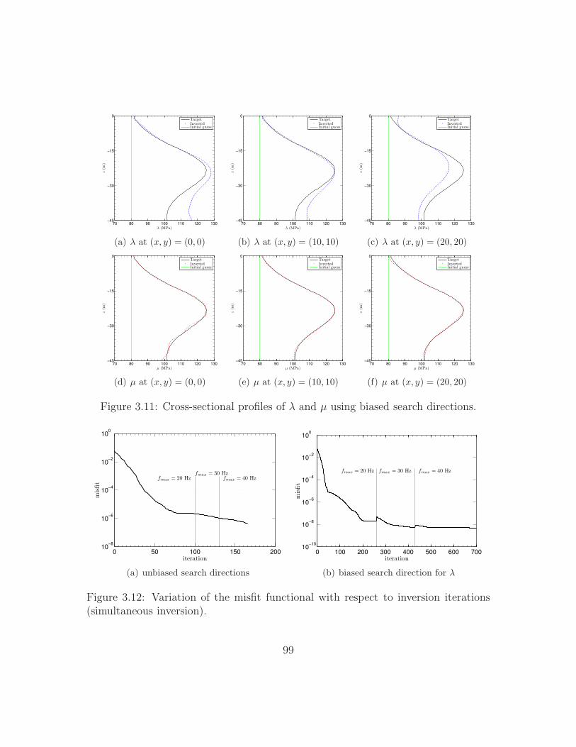
70 80 90 100 110 120 130−45
−30
−15
0
z(m
)
λ (MPa)
TargetInvertedInitial guess
(a) λ at (x, y) = (0, 0)
70 80 90 100 110 120 130−45
−30
−15
0
z(m
)λ (MPa)
TargetInvertedInitial guess
(b) λ at (x, y) = (10, 10)
70 80 90 100 110 120 130−45
−30
−15
0
z(m
)
λ (MPa)
TargetInvertedInitial guess
(c) λ at (x, y) = (20, 20)
70 80 90 100 110 120 130−45
−30
−15
0
z(m
)
µ (MPa)
TargetInvertedInitial guess
(d) µ at (x, y) = (0, 0)
70 80 90 100 110 120 130−45
−30
−15
0
z(m
)
µ (MPa)
TargetInvertedInitial guess
(e) µ at (x, y) = (10, 10)
70 80 90 100 110 120 130−45
−30
−15
0
z(m
)
µ (MPa)
TargetInvertedInitial guess
(f) µ at (x, y) = (20, 20)
Figure 3.11: Cross-sectional profiles of λ and µ using biased search directions.
0 50 100 150 20010
−8
10−6
10−4
10−2
100
iteration
misfit
fmax = 20 Hzfmax = 30 Hz
fmax = 40 Hz
(a) unbiased search directions
0 100 200 300 400 500 600 70010
−10
10−8
10−6
10−4
10−2
100
iteration
misfit
fmax = 20 Hz fmax = 30 Hz fmax = 40 Hz
(b) biased search direction for λ
Figure 3.12: Variation of the misfit functional with respect to inversion iterations(simultaneous inversion).
99
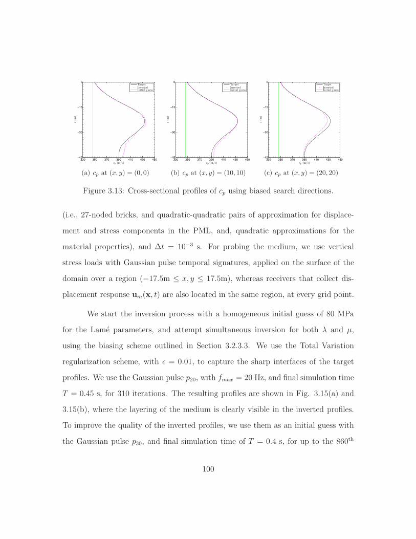
330 350 370 390 410 430 450−45
−30
−15
0
z(m
)
cp (m/s)
TargetInvertedInitial guess
(a) cp at (x, y) = (0, 0)
330 350 370 390 410 430 450−45
−30
−15
0
z(m
)
cp (m/s)
TargetInvertedInitial guess
(b) cp at (x, y) = (10, 10)
330 350 370 390 410 430 450−45
−30
−15
0
z(m
)
cp (m/s)
TargetInvertedInitial guess
(c) cp at (x, y) = (20, 20)
Figure 3.13: Cross-sectional profiles of cp using biased search directions.
(i.e., 27-noded bricks, and quadratic-quadratic pairs of approximation for displace-
ment and stress components in the PML, and, quadratic approximations for the
material properties), and ∆t = 10−3 s. For probing the medium, we use vertical
stress loads with Gaussian pulse temporal signatures, applied on the surface of the
domain over a region (−17.5m ≤ x, y ≤ 17.5m), whereas receivers that collect dis-
placement response um(x, t) are also located in the same region, at every grid point.
We start the inversion process with a homogeneous initial guess of 80 MPa
for the Lame parameters, and attempt simultaneous inversion for both λ and µ,
using the biasing scheme outlined in Section 3.2.3.3. We use the Total Variation
regularization scheme, with ǫ = 0.01, to capture the sharp interfaces of the target
profiles. We use the Gaussian pulse p20, with fmax = 20 Hz, and final simulation time
T = 0.45 s, for 310 iterations. The resulting profiles are shown in Fig. 3.15(a) and
3.15(b), where the layering of the medium is clearly visible in the inverted profiles.
To improve the quality of the inverted profiles, we use them as an initial guess with
the Gaussian pulse p30, and final simulation time of T = 0.4 s, for up to the 860th
100
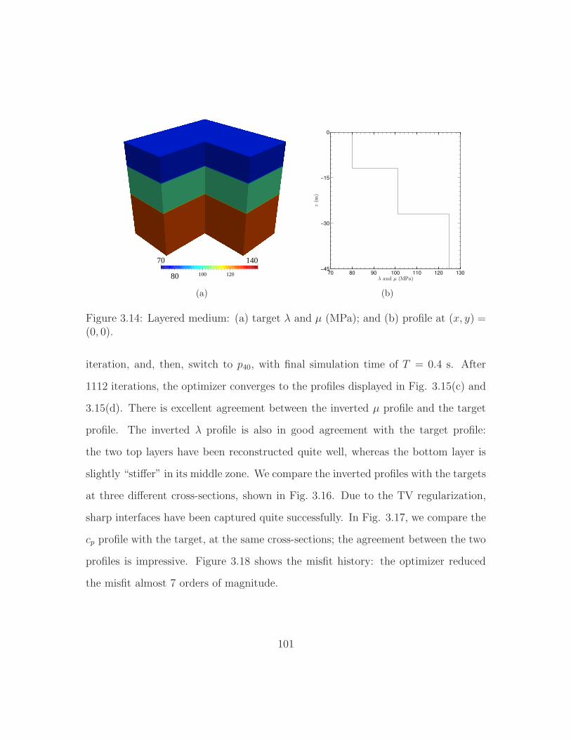
80 100 120
70 140
(a)
70 80 90 100 110 120 130−45
−30
−15
0
z(m
)
λ and µ (MPa)
(b)
Figure 3.14: Layered medium: (a) target λ and µ (MPa); and (b) profile at (x, y) =(0, 0).
iteration, and, then, switch to p40, with final simulation time of T = 0.4 s. After
1112 iterations, the optimizer converges to the profiles displayed in Fig. 3.15(c) and
3.15(d). There is excellent agreement between the inverted µ profile and the target
profile. The inverted λ profile is also in good agreement with the target profile:
the two top layers have been reconstructed quite well, whereas the bottom layer is
slightly “stiffer” in its middle zone. We compare the inverted profiles with the targets
at three different cross-sections, shown in Fig. 3.16. Due to the TV regularization,
sharp interfaces have been captured quite successfully. In Fig. 3.17, we compare the
cp profile with the target, at the same cross-sections; the agreement between the two
profiles is impressive. Figure 3.18 shows the misfit history: the optimizer reduced
the misfit almost 7 orders of magnitude.
101
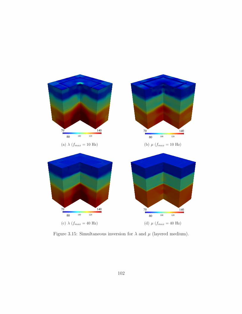
80 100 120
70 140
(a) λ (fmax = 10 Hz)
80 100 120
70 140
(b) µ (fmax = 10 Hz)
80 100 120
70 140
(c) λ (fmax = 40 Hz)
80 100 120
70 140
(d) µ (fmax = 40 Hz)
Figure 3.15: Simultaneous inversion for λ and µ (layered medium).
102
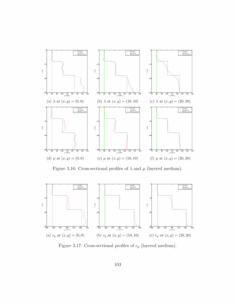
70 80 90 100 110 120 130 140 150−45
−30
−15
0
z(m
)
λ (MPa)
TargetInvertedInitial guess
(a) λ at (x, y) = (0, 0)
70 80 90 100 110 120 130 140 150−45
−30
−15
0
z(m
)λ (MPa)
TargetInvertedInitial guess
(b) λ at (x, y) = (10, 10)
70 80 90 100 110 120 130 140 150−45
−30
−15
0
z(m
)
λ (MPa)
TargetInvertedInitial guess
(c) λ at (x, y) = (20, 20)
70 80 90 100 110 120 130 140 150−45
−30
−15
0
z(m
)
µ (MPa)
TargetInvertedInitial guess
(d) µ at (x, y) = (0, 0)
70 80 90 100 110 120 130 140 150−45
−30
−15
0
z(m
)
µ (MPa)
TargetInvertedInitial guess
(e) µ at (x, y) = (10, 10)
70 80 90 100 110 120 130 140 150−45
−30
−15
0
z(m
)
µ (MPa)
TargetInvertedInitial guess
(f) µ at (x, y) = (20, 20)
Figure 3.16: Cross-sectional profiles of λ and µ (layered medium).
330 350 370 390 410 430 450−45
−30
−15
0
z(m
)
cp (m/s)
TargetInvertedInitial guess
(a) cp at (x, y) = (0, 0)
330 350 370 390 410 430 450−45
−30
−15
0
z(m
)
cp (m/s)
TargetInvertedInitial guess
(b) cp at (x, y) = (10, 10)
330 350 370 390 410 430 450−45
−30
−15
0
z(m
)
cp (m/s)
TargetInvertedInitial guess
(c) cp at (x, y) = (20, 20)
Figure 3.17: Cross-sectional profiles of cp (layered medium).
103
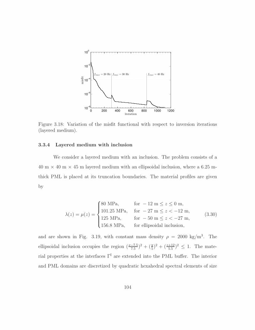
0 200 400 600 800 1000 120010
−8
10−6
10−4
10−2
100
iteration
misfit
fmax = 20 Hz fmax = 30 Hz fmax = 40 Hz
Figure 3.18: Variation of the misfit functional with respect to inversion iterations(layered medium).
3.3.4 Layered medium with inclusion
We consider a layered medium with an inclusion. The problem consists of a
40 m × 40 m × 45 m layered medium with an ellipsoidal inclusion, where a 6.25 m-
thick PML is placed at its truncation boundaries. The material profiles are given
by
λ(z) = µ(z) =
80 MPa, for − 12 m ≤ z ≤ 0 m,
101.25 MPa, for − 27 m ≤ z < −12 m,
125 MPa, for − 50 m ≤ z < −27 m,
156.8 MPa, for ellipsoidal inclusion,
(3.30)
and are shown in Fig. 3.19, with constant mass density ρ = 2000 kg/m3. The
ellipsoidal inclusion occupies the region (x−7.57.5
)2 + (y5)2 + ( z+12
5.5)2 ≤ 1. The mate-
rial properties at the interfaces ΓI are extended into the PML buffer. The interior
and PML domains are discretized by quadratic hexahedral spectral elements of size
104
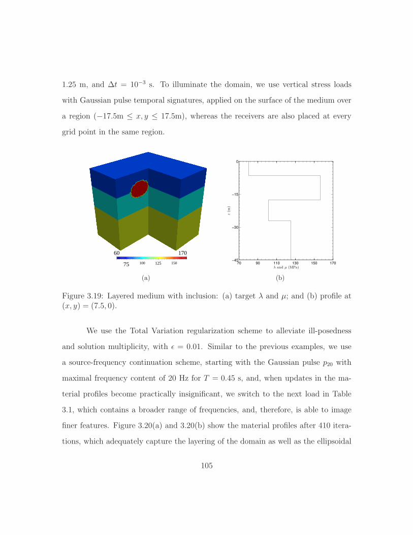
1.25 m, and ∆t = 10−3 s. To illuminate the domain, we use vertical stress loads
with Gaussian pulse temporal signatures, applied on the surface of the medium over
a region (−17.5m ≤ x, y ≤ 17.5m), whereas the receivers are also placed at every
grid point in the same region.
75 100 125 150
60 170
(a)
70 90 110 130 150 170−45
−30
−15
0
z(m
)
λ and µ (MPa)
(b)
Figure 3.19: Layered medium with inclusion: (a) target λ and µ; and (b) profile at(x, y) = (7.5, 0).
We use the Total Variation regularization scheme to alleviate ill-posedness
and solution multiplicity, with ǫ = 0.01. Similar to the previous examples, we use
a source-frequency continuation scheme, starting with the Gaussian pulse p20 with
maximal frequency content of 20 Hz for T = 0.45 s, and, when updates in the ma-
terial profiles become practically insignificant, we switch to the next load in Table
3.1, which contains a broader range of frequencies, and, therefore, is able to image
finer features. Figure 3.20(a) and 3.20(b) show the material profiles after 410 itera-
tions, which adequately capture the layering of the domain as well as the ellipsoidal
105
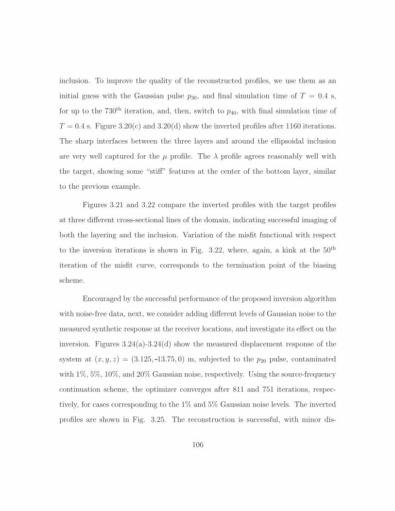
inclusion. To improve the quality of the reconstructed profiles, we use them as an
initial guess with the Gaussian pulse p30, and final simulation time of T = 0.4 s,
for up to the 730th iteration, and, then, switch to p40, with final simulation time of
T = 0.4 s. Figure 3.20(c) and 3.20(d) show the inverted profiles after 1160 iterations.
The sharp interfaces between the three layers and around the ellipsoidal inclusion
are very well captured for the µ profile. The λ profile agrees reasonably well with
the target, showing some “stiff” features at the center of the bottom layer, similar
to the previous example.
Figures 3.21 and 3.22 compare the inverted profiles with the target profiles
at three different cross-sectional lines of the domain, indicating successful imaging of
both the layering and the inclusion. Variation of the misfit functional with respect
to the inversion iterations is shown in Fig. 3.22, where, again, a kink at the 50th
iteration of the misfit curve, corresponds to the termination point of the biasing
scheme.
Encouraged by the successful performance of the proposed inversion algorithm
with noise-free data, next, we consider adding different levels of Gaussian noise to the
measured synthetic response at the receiver locations, and investigate its effect on the
inversion. Figures 3.24(a)-3.24(d) show the measured displacement response of the
system at (x, y, z) = (3.125, 13.75, 0) m, subjected to the p20 pulse, contaminated
with 1%, 5%, 10%, and 20% Gaussian noise, respectively. Using the source-frequency
continuation scheme, the optimizer converges after 811 and 751 iterations, respec-
tively, for cases corresponding to the 1% and 5% Gaussian noise levels. The inverted
profiles are shown in Fig. 3.25. The reconstruction is successful, with minor dis-
106
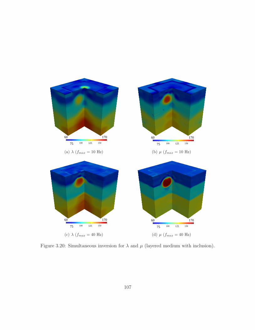
75 100 125 150
60 170
(a) λ (fmax = 10 Hz)
75 100 125 150
60 170
(b) µ (fmax = 10 Hz)
75 100 125 150
60 170
(c) λ (fmax = 40 Hz)
75 100 125 150
60 170
(d) µ (fmax = 40 Hz)
Figure 3.20: Simultaneous inversion for λ and µ (layered medium with inclusion).
107
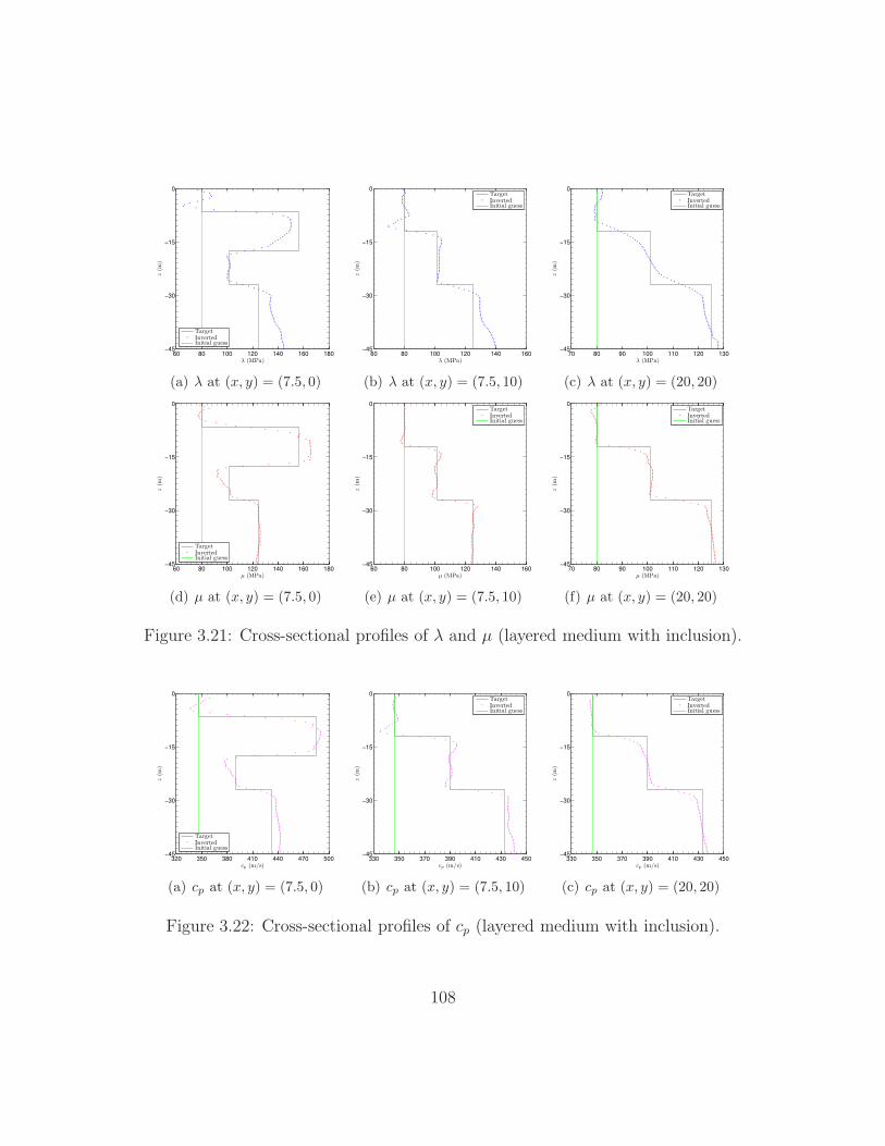
60 80 100 120 140 160 180−45
−30
−15
0
z(m
)
λ (MPa)
TargetInvertedInitial guess
(a) λ at (x, y) = (7.5, 0)
60 80 100 120 140 160−45
−30
−15
0
z(m
)λ (MPa)
TargetInvertedInitial guess
(b) λ at (x, y) = (7.5, 10)
70 80 90 100 110 120 130−45
−30
−15
0
z(m
)
λ (MPa)
TargetInvertedInitial guess
(c) λ at (x, y) = (20, 20)
60 80 100 120 140 160 180−45
−30
−15
0
z(m
)
µ (MPa)
TargetInvertedInitial guess
(d) µ at (x, y) = (7.5, 0)
60 80 100 120 140 160−45
−30
−15
0
z(m
)
µ (MPa)
TargetInvertedInitial guess
(e) µ at (x, y) = (7.5, 10)
70 80 90 100 110 120 130−45
−30
−15
0
z(m
)
µ (MPa)
TargetInvertedInitial guess
(f) µ at (x, y) = (20, 20)
Figure 3.21: Cross-sectional profiles of λ and µ (layered medium with inclusion).
320 350 380 410 440 470 500−45
−30
−15
0
z(m
)
cp (m/s)
TargetInvertedInitial guess
(a) cp at (x, y) = (7.5, 0)
330 350 370 390 410 430 450−45
−30
−15
0
z(m
)
cp (m/s)
TargetInvertedInitial guess
(b) cp at (x, y) = (7.5, 10)
330 350 370 390 410 430 450−45
−30
−15
0
z(m
)
cp (m/s)
TargetInvertedInitial guess
(c) cp at (x, y) = (20, 20)
Figure 3.22: Cross-sectional profiles of cp (layered medium with inclusion).
108
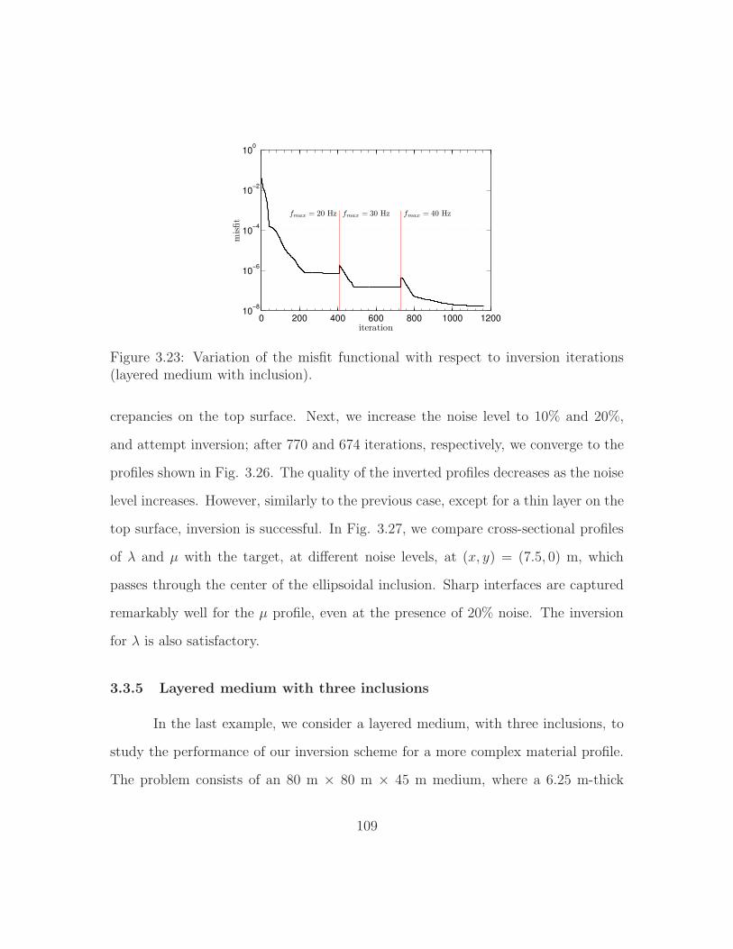
0 200 400 600 800 1000 120010
−8
10−6
10−4
10−2
100
iteration
misfit
fmax = 20 Hz fmax = 30 Hz fmax = 40 Hz
Figure 3.23: Variation of the misfit functional with respect to inversion iterations(layered medium with inclusion).
crepancies on the top surface. Next, we increase the noise level to 10% and 20%,
and attempt inversion; after 770 and 674 iterations, respectively, we converge to the
profiles shown in Fig. 3.26. The quality of the inverted profiles decreases as the noise
level increases. However, similarly to the previous case, except for a thin layer on the
top surface, inversion is successful. In Fig. 3.27, we compare cross-sectional profiles
of λ and µ with the target, at different noise levels, at (x, y) = (7.5, 0) m, which
passes through the center of the ellipsoidal inclusion. Sharp interfaces are captured
remarkably well for the µ profile, even at the presence of 20% noise. The inversion
for λ is also satisfactory.
3.3.5 Layered medium with three inclusions
In the last example, we consider a layered medium, with three inclusions, to
study the performance of our inversion scheme for a more complex material profile.
The problem consists of an 80 m × 80 m × 45 m medium, where a 6.25 m-thick
109
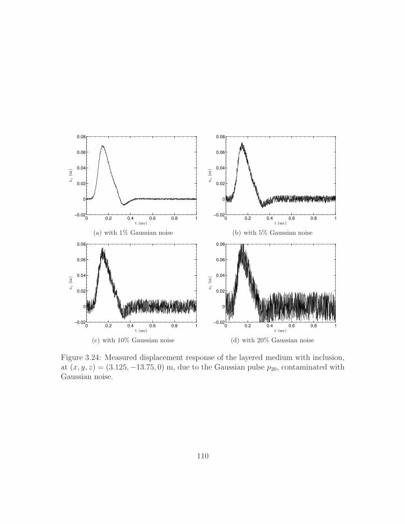
0 0.2 0.4 0.6 0.8 1−0.02
0
0.02
0.04
0.06
0.08
t (sec)
uz
(m)
(a) with 1% Gaussian noise
0 0.2 0.4 0.6 0.8 1−0.02
0
0.02
0.04
0.06
0.08
t (sec)
uz
(m)
(b) with 5% Gaussian noise
0 0.2 0.4 0.6 0.8 1−0.02
0
0.02
0.04
0.06
0.08
t (sec)
uz
(m)
(c) with 10% Gaussian noise
0 0.2 0.4 0.6 0.8 1−0.02
0
0.02
0.04
0.06
0.08
t (sec)
uz
(m)
(d) with 20% Gaussian noise
Figure 3.24: Measured displacement response of the layered medium with inclusion,at (x, y, z) = (3.125,−13.75, 0) m, due to the Gaussian pulse p20, contaminated withGaussian noise.
110
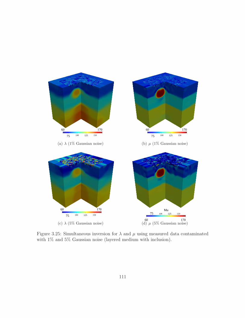
75 100 125 150
60 170
(a) λ (1% Gaussian noise)
75 100 125 150
60 170
(b) µ (1% Gaussian noise)
75 100 125 150
60 170
(c) λ (5% Gaussian noise)
75 100 125 150
Mu
60 170(d) µ (5% Gaussian noise)
Figure 3.25: Simultaneous inversion for λ and µ using measured data contaminatedwith 1% and 5% Gaussian noise (layered medium with inclusion).
111
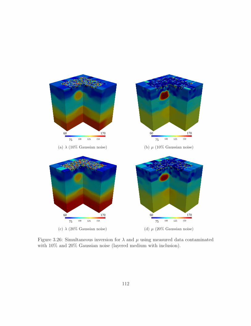
75 100 125 150
60 170
(a) λ (10% Gaussian noise)
75 100 125 150
60 170
(b) µ (10% Gaussian noise)
75 100 125 150
60 170
(c) λ (20% Gaussian noise)
75 100 125 150
60 170
(d) µ (20% Gaussian noise)
Figure 3.26: Simultaneous inversion for λ and µ using measured data contaminatedwith 10% and 20% Gaussian noise (layered medium with inclusion).
112
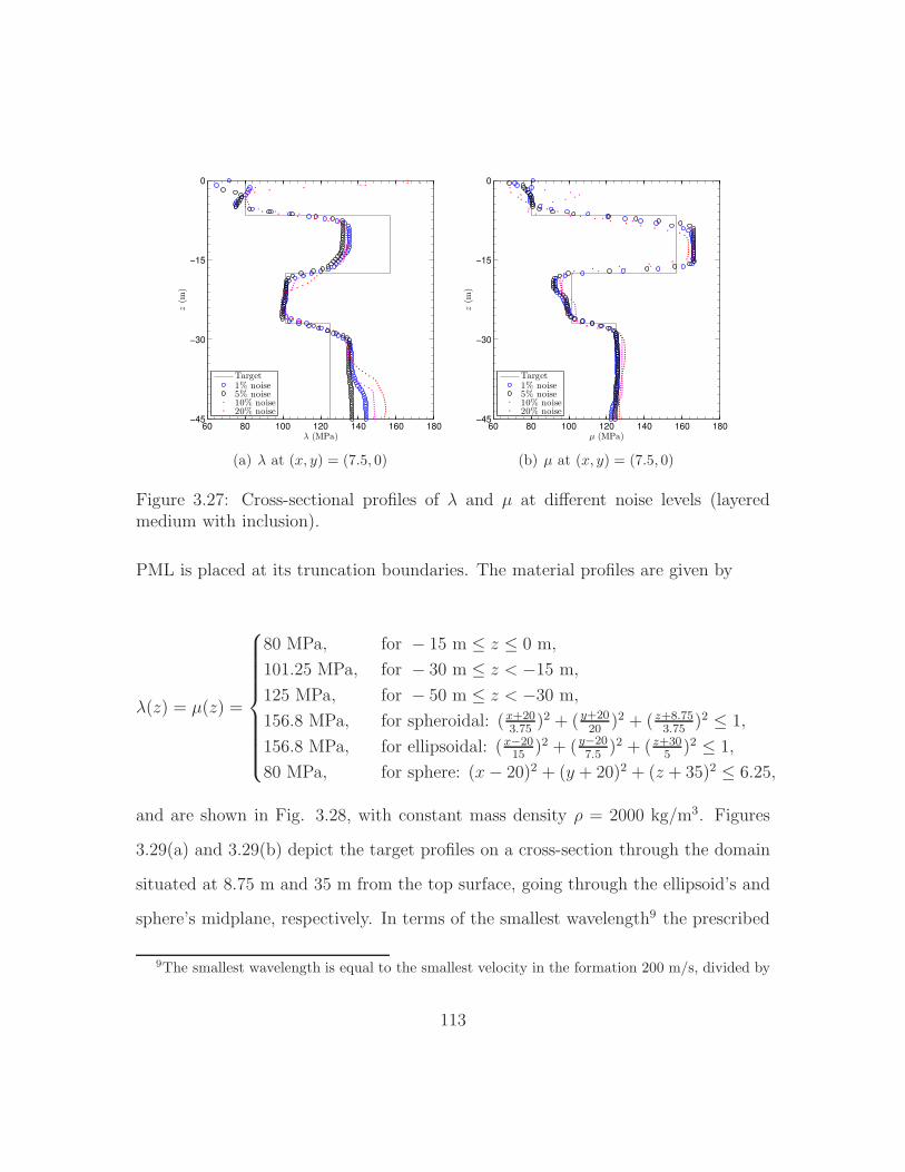
60 80 100 120 140 160 180−45
−30
−15
0z
(m)
λ (MPa)
Target1% noise5% noise10% noise20% noise
(a) λ at (x, y) = (7.5, 0)
60 80 100 120 140 160 180−45
−30
−15
0
z(m
)
µ (MPa)
Target1% noise5% noise10% noise20% noise
(b) µ at (x, y) = (7.5, 0)
Figure 3.27: Cross-sectional profiles of λ and µ at different noise levels (layeredmedium with inclusion).
PML is placed at its truncation boundaries. The material profiles are given by
λ(z) = µ(z) =
80 MPa, for − 15 m ≤ z ≤ 0 m,
101.25 MPa, for − 30 m ≤ z < −15 m,
125 MPa, for − 50 m ≤ z < −30 m,
156.8 MPa, for spheroidal: (x+203.75
)2 + (y+2020
)2 + ( z+8.753.75
)2 ≤ 1,
156.8 MPa, for ellipsoidal: (x−2015
)2 + (y−207.5
)2 + ( z+305
)2 ≤ 1,
80 MPa, for sphere: (x− 20)2 + (y + 20)2 + (z + 35)2 ≤ 6.25,
and are shown in Fig. 3.28, with constant mass density ρ = 2000 kg/m3. Figures
3.29(a) and 3.29(b) depict the target profiles on a cross-section through the domain
situated at 8.75 m and 35 m from the top surface, going through the ellipsoid’s and
sphere’s midplane, respectively. In terms of the smallest wavelength9 the prescribed
9The smallest wavelength is equal to the smallest velocity in the formation 200 m/s, divided by
113
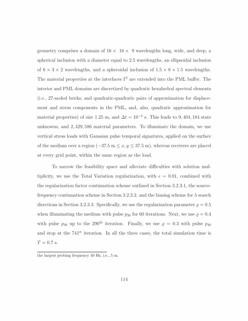
geometry comprises a domain of 16 × 16 × 9 wavelengths long, wide, and deep, a
spherical inclusion with a diameter equal to 2.5 wavelengths, an ellipsoidal inclusion
of 6 × 3 × 2 wavelengths, and a spheroidal inclusion of 1.5 × 8 × 1.5 wavelengths.
The material properties at the interfaces ΓI are extended into the PML buffer. The
interior and PML domains are discretized by quadratic hexahedral spectral elements
(i.e., 27-noded bricks, and quadratic-quadratic pairs of approximation for displace-
ment and stress components in the PML, and, also, quadratic approximation for
material properties) of size 1.25 m, and ∆t = 10−3 s. This leads to 9, 404, 184 state
unknowns, and 2, 429, 586 material parameters. To illuminate the domain, we use
vertical stress loads with Gaussian pulse temporal signatures, applied on the surface
of the medium over a region (−37.5 m ≤ x, y ≤ 37.5 m), whereas receivers are placed
at every grid point, within the same region as the load.
To narrow the feasibility space and alleviate difficulties with solution mul-
tiplicity, we use the Total Variation regularization, with ǫ = 0.01, combined with
the regularization factor continuation scheme outlined in Section 3.2.3.1, the source-
frequency continuation scheme in Section 3.2.3.2, and the biasing scheme for λ search
directions in Section 3.2.3.3. Specifically, we use the regularization parameter = 0.5
when illuminating the medium with pulse p20 for 60 iterations. Next, we use = 0.4
with pulse p30 up to the 290th iteration. Finally, we use = 0.3 with pulse p40
and stop at the 741st iteration. In all the three cases, the total simulation time is
T = 0.7 s.
the largest probing frequency 40 Hz, i.e., 5 m.
114
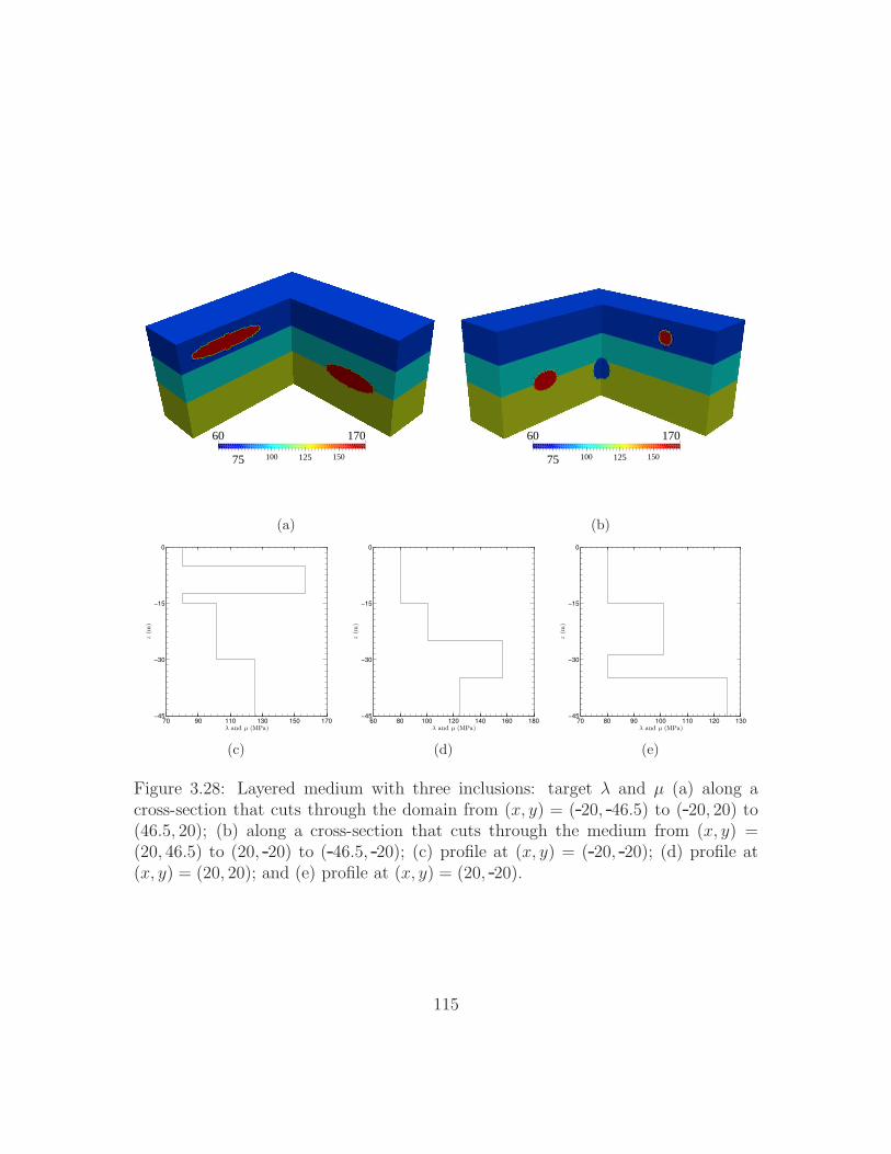
75 100 125 150
60 170
(a)
75 100 125 150
60 170
(b)
70 90 110 130 150 170−45
−30
−15
0
z(m
)
λ and µ (MPa)
(c)
60 80 100 120 140 160 180−45
−30
−15
0
z(m
)
λ and µ (MPa)
(d)
70 80 90 100 110 120 130−45
−30
−15
0
z(m
)
λ and µ (MPa)
(e)
Figure 3.28: Layered medium with three inclusions: target λ and µ (a) along across-section that cuts through the domain from (x, y) = ( 20, 46.5) to ( 20, 20) to(46.5, 20); (b) along a cross-section that cuts through the medium from (x, y) =(20, 46.5) to (20, 20) to ( 46.5, 20); (c) profile at (x, y) = ( 20, 20); (d) profile at(x, y) = (20, 20); and (e) profile at (x, y) = (20, 20).
115
75 100 125 150
60 170
(a)
80 100 120
70 140
(b)
Figure 3.29: Layered medium with three inclusions: target λ and µ on (a) thez = −8.75 m cross-section; and (b) the z = −35 m cross-section.
Figure 3.30 shows the inverted profile along a cross-section that cuts through
the domain from (x, y) = ( 20, 46.5) to ( 20, 20) to (46.5, 20). The cross section
passes through the larger semi-principal axes of both ellipsoids, and shows very good
reconstruction of the µ profile, and satisfactory inversion of the λ profile. The layering
is sharp, and the ellipsoids are captured well. In Fig. 3.31, a cross section of the
inverted profiles from (x, y) = (20, 46.5) to (20, 20) to ( 46.5, 20) is displayed, where
it passes through the smaller semi-principal axes of the ellipsoids and the center of
the sphere. The ellipsoids are well captured; however, the sphere, which consists of
“soft” materials, can hardly be noticed, especially, in the λ profile. Figure 3.32(a) and
3.32(b) show the inverted profiles on a cross-section through the domain, situated
at 8.75 m from the surface, going through the top ellipsoid’s midplane, and show
satisfactory reconstruction of the ellipsoid. To see the reconstruction of the sphere
116
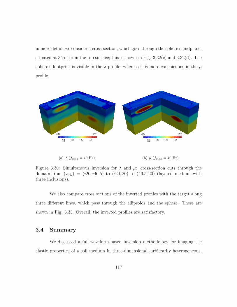
in more detail, we consider a cross-section, which goes through the sphere’s midplane,
situated at 35 m from the top surface; this is shown in Fig. 3.32(c) and 3.32(d). The
sphere’s footprint is visible in the λ profile, whereas it is more conspicuous in the µ
profile.
75 100 125 150
60 170
(a) λ (fmax = 40 Hz)
75 100 125 150
60 170
(b) µ (fmax = 40 Hz)
Figure 3.30: Simultaneous inversion for λ and µ: cross-section cuts through thedomain from (x, y) = ( 20, 46.5) to ( 20, 20) to (46.5, 20) (layered medium withthree inclusions).
We also compare cross sections of the inverted profiles with the target along
three different lines, which pass through the ellipsoids and the sphere. These are
shown in Fig. 3.33. Overall, the inverted profiles are satisfactory.
3.4 Summary
We discussed a full-waveform-based inversion methodology for imaging the
elastic properties of a soil medium in three-dimensional, arbitrarily heterogeneous,
117
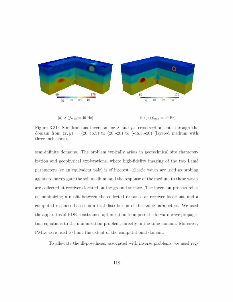
75 100 125 150
60 170
(a) λ (fmax = 40 Hz)
75 100 125 150
60 170
(b) µ (fmax = 40 Hz)
Figure 3.31: Simultaneous inversion for λ and µ: cross-section cuts through thedomain from (x, y) = (20, 46.5) to (20, 20) to ( 46.5, 20) (layered medium withthree inclusions).
semi-infinite domains. The problem typically arises in geotechnical site character-
ization and geophysical explorations, where high-fidelity imaging of the two Lame
parameters (or an equivalent pair) is of interest. Elastic waves are used as probing
agents to interrogate the soil medium, and the response of the medium to these waves
are collected at receivers located on the ground surface. The inversion process relies
on minimizing a misfit between the collected response at receiver locations, and a
computed response based on a trial distribution of the Lame parameters. We used
the apparatus of PDE-constrained optimization to impose the forward wave propaga-
tion equations to the minimization problem, directly in the time-domain. Moreover,
PMLs were used to limit the extent of the computational domain.
To alleviate the ill-posedness, associated with inverse problems, we used reg-
118
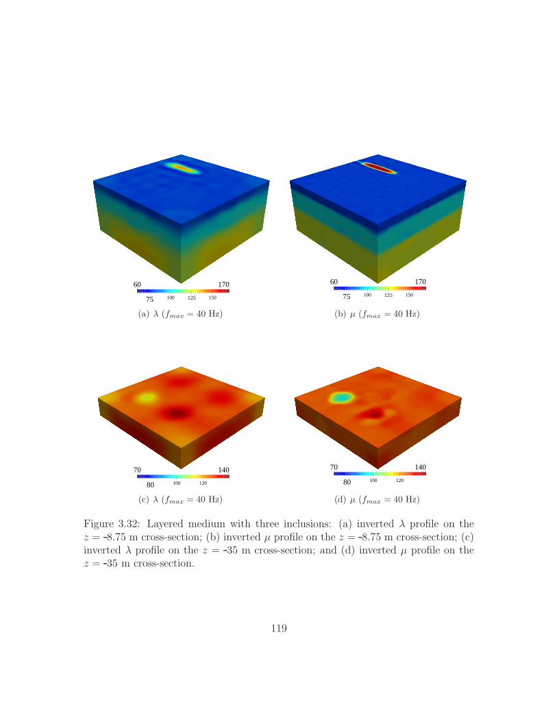
75 100 125 150
60 170
(a) λ (fmax = 40 Hz)
75 100 125 150
60 170
(b) µ (fmax = 40 Hz)
80 100 120
70 140
(c) λ (fmax = 40 Hz)
80 100 120
70 140
(d) µ (fmax = 40 Hz)
Figure 3.32: Layered medium with three inclusions: (a) inverted λ profile on thez = 8.75 m cross-section; (b) inverted µ profile on the z = 8.75 m cross-section; (c)inverted λ profile on the z = 35 m cross-section; and (d) inverted µ profile on thez = 35 m cross-section.
119
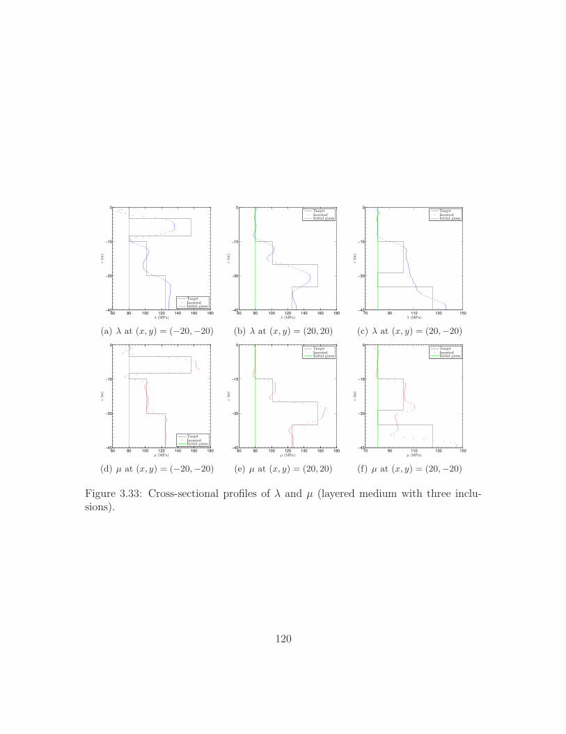
60 80 100 120 140 160 180−45
−30
−15
0
z(m
)
λ (MPa)
TargetInvertedInitial guess
(a) λ at (x, y) = (−20,−20)
60 80 100 120 140 160 180−45
−30
−15
0
z(m
)
λ (MPa)
TargetInvertedInitial guess
(b) λ at (x, y) = (20, 20)
70 90 110 130 150−45
−30
−15
0
z(m
)
λ (MPa)
TargetInvertedInitial guess
(c) λ at (x, y) = (20,−20)
60 80 100 120 140 160 180−45
−30
−15
0
z(m
)
µ (MPa)
TargetInvertedInitial guess
(d) µ at (x, y) = (−20,−20)
60 80 100 120 140 160 180−45
−30
−15
0
z(m
)
µ (MPa)
TargetInvertedInitial guess
(e) µ at (x, y) = (20, 20)
70 90 110 130 150−45
−30
−15
0
z(m
)
µ (MPa)
TargetInvertedInitial guess
(f) µ at (x, y) = (20,−20)
Figure 3.33: Cross-sectional profiles of λ and µ (layered medium with three inclu-sions).
120

ularization schemes, along with a regularization factor continuation scheme, which
tunes the regularization factor adaptively at each inversion iteration. We discussed
additional strategies to robustify the inversion algorithm: specifically, we used (a)
a source-frequency continuation scheme such that the inversion process evolves by
using low-frequency sources, and, gradually, we use sources with higher frequencies;
and (b) a biasing scheme for the λ-profile, such that, at early iterations of inversion,
the search direction for λ is biased based on that of µ. The latter strategy, in particu-
lar, improves the reconstruction of the material profiles when simultaneous inversion
of the two Lame parameters is exercised. To the best of our knowledge, this is the
first attempt that the two Lame parameters have been successfully reconstructed in
three-dimensional PML-truncated domains.
By comparing directional finite differences of the discrete objective functional,
and directional derivatives obtained via the control problems, we verified the accuracy
and correctness of the material gradients. We reported numerical results demonstrat-
ing successful reconstruction of both Lame parameters for smooth and sharp profiles.
Overall, the framework discussed in this study seems robust, practical, and promis-
ing.
121
Chapter 4
Site characterization using full-waveform inversion
In the preceding chapters, we discussed the theoretical aspects of a full-
waveform-inversion-based methodology for the imaging of the elastic properties of
near-surface deposits. We also addressed the forward problem of numerically simu-
lating the propagation of waves in PML-truncated, arbitrarily heterogeneous, elastic
domains. We presented several PML formulations for the three-dimensional case, nu-
merical results for the forward problem, as well as numerical results for the associated
inverse medium problem using synthetic data.
In this chapter, we focus on the exercising of the developed methodology by
real, as opposed to synthetic, data. There are several applications in engineering
that stand to benefit from a robust full-waveform-inversion methodology: among
these, our focus here is geotechnical site characterization. To this end, we use the
data collected during two field experiments in an attempt to validate the theoretical
development. Specifically, we consider two cases consistent with our code develop-
ment cycle: firstly, we describe the design of a field experiment aimed at reproducing
in the field plane-strain conditions, in order to allow us to exercise two-dimensional
inversion codes. We describe the design, the pre-processing, the field data, and the
inversion results. Moreover, we describe comparisons of the inverted full-waveform
122
based profile against those by using two other imaging methods - the non-invasive
SASW, as well as an invasive CPT test. Secondly, we describe the field experi-
ment and associated inversion results obtained by exercising the three-dimensional
inversion codes.
The remainder of this chapter is organized as follows: first, we review the
mathematical and numerical aspects of the underlying inverse medium problem in
two space dimensions. We remark that there are differences between the two- and
three-dimensional formulation that merit a detailed discussion. The differences stem
from the fact that the number of stretching functions for the PML equals the spatial
dimensionality: this difference, in turn, affects the temporal complexity, and gives
rise to alternative formulations, which could not be trivially obtained by simply re-
ducing the three-dimensional formulations to two dimensions. The two-dimensional
development preceded the research described in this dissertation [57]. However, algo-
rithmic modifications/improvements, the field experiment, and the two-dimensional
inversion results using the field data were all part of the work described herein. Next,
we describe the design, data collection, and full-waveform inversion results based on
a field experiment collected at the UCSB NEES site in Garner Valley, California in
March 2012. Lastly, we conclude with summary remarks.
4.1 The inverse medium problem in two space dimensions
To fix ideas, we refer to the depiction of the driving application shown in
Fig. 4.1: similarly to the three-dimensional case, here too we are interested in recon-
structing the formation’s profile shown in Fig. 4.1(a). Given the arbitrary heterogene-
123
ity of the domain of interest, the problem is inherently three-dimensional. Herein, we
describe the methodology by focusing on the two-dimensional counterpart of the orig-
inal problem, as depicted in Fig. 4.1(b): we accept arbitrary heterogeneity within
a two-dimensional slice, but presume that the properties remain unchanged along
the third dimension, i.e., a plane strain problem. While, the problem, as defined,
departs from the true physical three-dimensional case1, it still contains all the algo-
rithmic and theoretical complexities associated with the three-dimensional problem.
Figure 4.1(c) represents the mathematical idealization of the two-dimensional slice
shown in Fig. 4.1(b): the semi-infinite (two-dimensional) physical domain has been
truncated to a finite one, through the introduction of PMLs.
4.1.1 The forward problem
We use a hybrid approach for the simulation of the wave motion inside a two-
dimensional PML-truncated elastic medium. We refer to [33] and references therein
for the complete development of the method. Here, we repeat only the resulting
coupled system of equations. Accordingly, find u(x, t) in ΩRD ∪ΩPML, and S(x, t) in
ΩPML (see Fig. 4.2 for domain and boundary designations), where u and S reside in
appropriate functional spaces and:
1The problem is still valid in the case of horizontal layers, or even in the case of inclined layers,or even in the case of arbitrary plane heterogeneity.
124
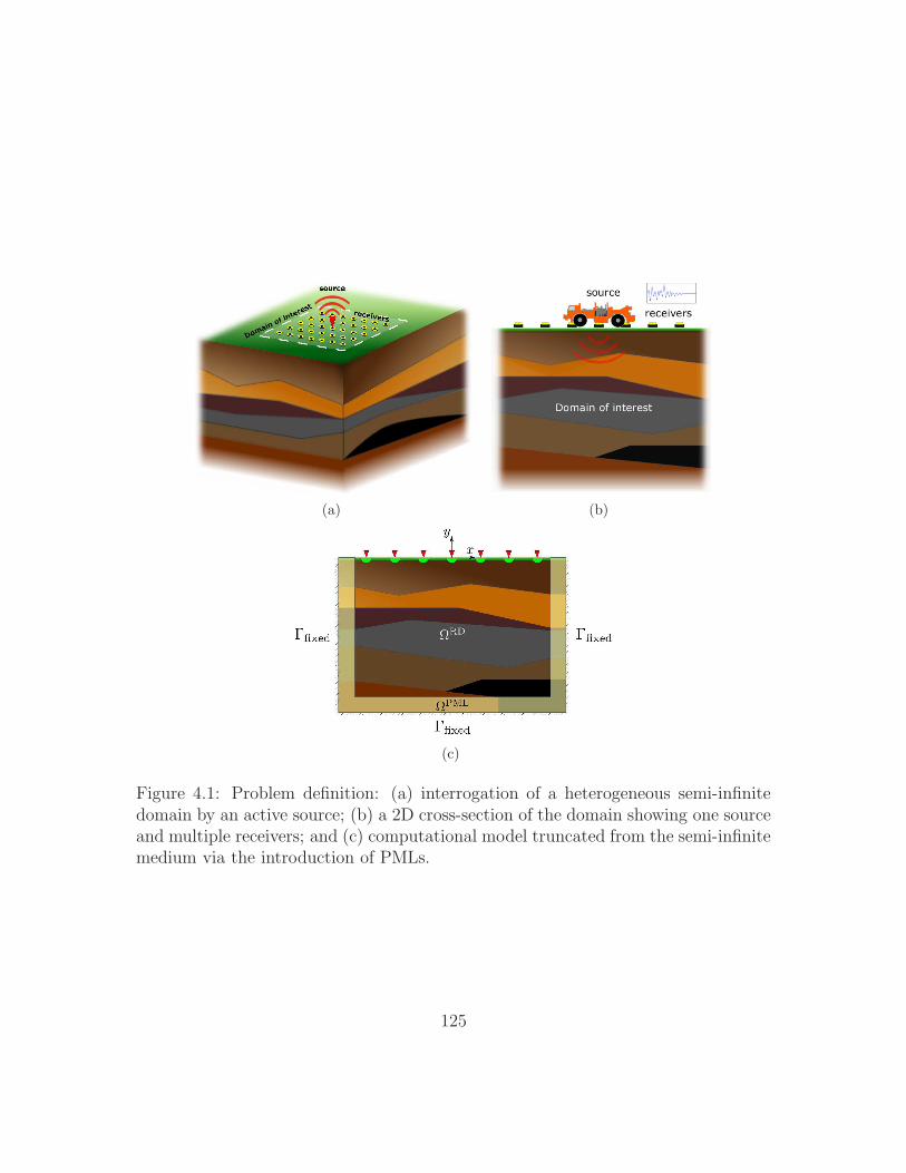
(a) (b)
(c)
Figure 4.1: Problem definition: (a) interrogation of a heterogeneous semi-infinitedomain by an active source; (b) a 2D cross-section of the domain showing one sourceand multiple receivers; and (c) computational model truncated from the semi-infinitemedium via the introduction of PMLs.
125
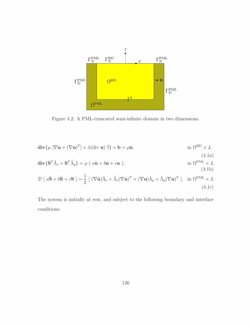
n
z
Figure 4.2: A PML-truncated semi-infinite domain in two dimensions.
divµ [∇u+ (∇u)T ] + λ(div u) I+ b = ρu, in ΩRD × J,
(4.1a)
divST Λe + ST Λp = ρ ( au+ bu+ cu ), in ΩPML × J,(4.1b)
D [ aS+ bS+ cS ] =1
2[ (∇u)Λe + Λe(∇u)T + (∇u)Λp + Λp(∇u)T ], in ΩPML × J.
(4.1c)
The system is initially at rest, and subject to the following boundary and interface
conditions:
126
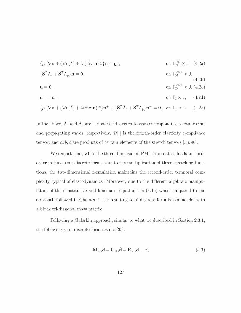
µ [∇u+ (∇u)T ] + λ (div u) In = gn, on ΓRDN × J, (4.2a)
ST Λe + ST Λpn = 0, on ΓPMLN × J,
(4.2b)
u = 0, on ΓPMLD × J, (4.2c)
u+ = u−, on ΓI × J, (4.2d)
µ [∇u+ (∇u)T ] + λ(div u) In+ + ST Λe + ST Λpn− = 0, on ΓI × J. (4.2e)
In the above, Λe and Λp are the so-called stretch tensors corresponding to evanescent
and propagating waves, respectively, D[·] is the fourth-order elasticity compliance
tensor, and a, b, c are products of certain elements of the stretch tensors [33, 96].
We remark that, while the three-dimensional PML formulation leads to third-
order in time semi-discrete forms, due to the multiplication of three stretching func-
tions, the two-dimensional formulation maintains the second-order temporal com-
plexity typical of elastodynamics. Moreover, due to the different algebraic manipu-
lation of the constitutive and kinematic equations in (4.1c) when compared to the
approach followed in Chapter 2, the resulting semi-discrete form is symmetric, with
a block tri-diagonal mass matrix.
Following a Galerkin approach, similar to what we described in Section 2.3.1,
the following semi-discrete form results [33]:
M2Dd+C2Dd+K2Dd = f , (4.3)
127
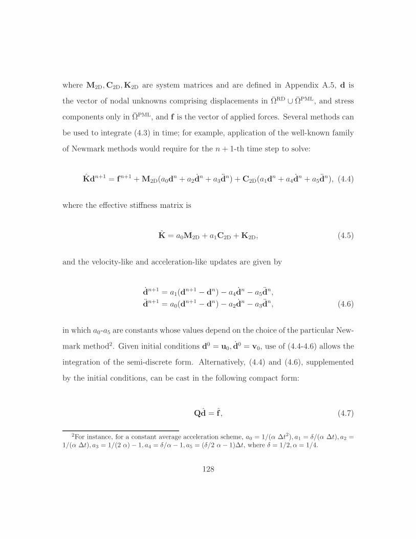
where M2D,C2D,K2D are system matrices and are defined in Appendix A.5, d is
the vector of nodal unknowns comprising displacements in ΩRD ∪ ΩPML, and stress
components only in ΩPML, and f is the vector of applied forces. Several methods can
be used to integrate (4.3) in time; for example, application of the well-known family
of Newmark methods would require for the n+ 1-th time step to solve:
Kdn+1 = fn+1 +M2D(a0dn + a2d
n + a3dn) +C2D(a1d
n + a4dn + a5d
n), (4.4)
where the effective stiffness matrix is
K = a0M2D + a1C2D +K2D, (4.5)
and the velocity-like and acceleration-like updates are given by
dn+1 = a1(dn+1 − dn)− a4d
n − a5dn,
dn+1 = a0(dn+1 − dn)− a2d
n − a3dn, (4.6)
in which a0-a5 are constants whose values depend on the choice of the particular New-
mark method2. Given initial conditions d0 = u0, d0 = v0, use of (4.4-4.6) allows the
integration of the semi-discrete form. Alternatively, (4.4) and (4.6), supplemented
by the initial conditions, can be cast in the following compact form:
Qd = f , (4.7)
2For instance, for a constant average acceleration scheme, a0 = 1/(α ∆t2), a1 = δ/(α ∆t), a2 =1/(α ∆t), a3 = 1/(2 α)− 1, a4 = δ/α− 1, a5 = (δ/2 α− 1)∆t, where δ = 1/2, α = 1/4.
128
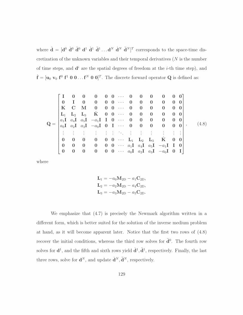
where d = [d0 d0 d0 d1 d1 d1 . . .dN dN dN ]T corresponds to the space-time dis-
cretization of the unknown variables and their temporal derivatives (N is the number
of time steps, and di are the spatial degrees of freedom at the i-th time step), and
f = [u0 v0 f0 f1 0 0 . . . fN 0 0]T . The discrete forward operator Q is defined as:
Q =
I 0 0 0 0 0 · · · 0 0 0 0 0 00 I 0 0 0 0 · · · 0 0 0 0 0 0K C M 0 0 0 · · · 0 0 0 0 0 0
L1 L2 L3 K 0 0 · · · 0 0 0 0 0 0a1I a4I a5I −a1I I 0 · · · 0 0 0 0 0 0a0I a2I a3I −a0I 0 I · · · 0 0 0 0 0 0...
......
......
.... . .
......
......
......
0 0 0 0 0 0 · · · L1 L2 L3 K 0 00 0 0 0 0 0 · · · a1I a4I a5I −a1I I 00 0 0 0 0 0 · · · a0I a2I a3I −a0I 0 I
, (4.8)
where
L1 = −a0M2D − a1C2D,
L2 = −a2M2D − a4C2D,
L3 = −a3M2D − a5C2D.
We emphasize that (4.7) is precisely the Newmark algorithm written in a
different form, which is better suited for the solution of the inverse medium problem
at hand, as it will become apparent later. Notice that the first two rows of (4.8)
recover the initial conditions, whereas the third row solves for d0. The fourth row
solves for d1, and the fifth and sixth rows yield d1, d1, respectively. Finally, the last
three rows, solve for dN , and update dN , dN , respectively.
129
4.1.2 The inverse problem
We consider the following PDE-constrained minimization problem:
minλ,µ
J(λ, µ) :=1
2
Nr∑
j=1
∫ T
0
∫
Γm
(u− um)2 δ(x− xj) ds(x) dt+ RTN(λ, µ), (4.9)
subject to the (continuous) forward problem governed by the initial- and boundary-
value problem (4.1a)-(4.2e).
In the above, u is the vertical component of the computed displacement,
and um corresponds to the measured vertical displacement component (obtained via
sensor data processing).
One may use the (formal) Lagrangian approach [86], whereby the forward
problem (4.1a)-(4.2e) is imposed via Lagrange multipliers (adjoint variables) to the
functional (4.9). One then seeks a stationary point to the resulting Lagrangian
functional, by forcing the first-order optimality conditions to vanish. This approach
was discussed in detail in Chapter 3, and is referred to as an optimize-then-discretize
approach, since the optimality conditions are sought first in their continuous form,
followed by spatial and temporal discretization steps3.
Alternatively, one may discretize the continuous constrained optimization
problem (4.9) first, and then compute the corresponding discrete optimality con-
ditions [68, 94]. The procedure is referred to as a discretize-then-optimize approach
3See also [57].
130
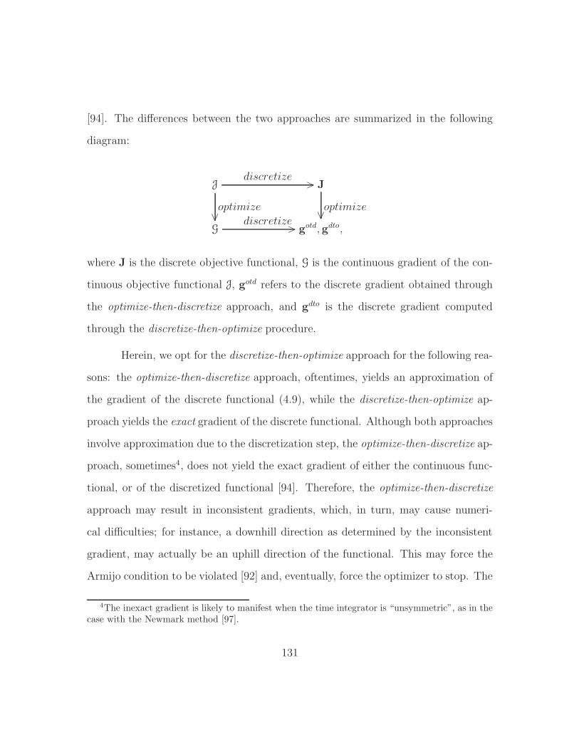
[94]. The differences between the two approaches are summarized in the following
diagram:
Jdiscretize
> J
G
optimize∨ discretize
> gotd, gdto,
optimize∨
where J is the discrete objective functional, G is the continuous gradient of the con-
tinuous objective functional J, gotd refers to the discrete gradient obtained through
the optimize-then-discretize approach, and gdto is the discrete gradient computed
through the discretize-then-optimize procedure.
Herein, we opt for the discretize-then-optimize approach for the following rea-
sons: the optimize-then-discretize approach, oftentimes, yields an approximation of
the gradient of the discrete functional (4.9), while the discretize-then-optimize ap-
proach yields the exact gradient of the discrete functional. Although both approaches
involve approximation due to the discretization step, the optimize-then-discretize ap-
proach, sometimes4, does not yield the exact gradient of either the continuous func-
tional, or of the discretized functional [94]. Therefore, the optimize-then-discretize
approach may result in inconsistent gradients, which, in turn, may cause numeri-
cal difficulties; for instance, a downhill direction as determined by the inconsistent
gradient, may actually be an uphill direction of the functional. This may force the
Armijo condition to be violated [92] and, eventually, force the optimizer to stop. The
4The inexact gradient is likely to manifest when the time integrator is “unsymmetric”, as in thecase with the Newmark method [97].
131
discretize-then-optimize approach, however, is more robust and does not suffer from
such problems (see, for example, Chapter 4 in [94] for a comprehensive discussion
and [68] for a systematic treatment and a detailed example).
Discrete optimality conditions
Discretization of the objective functional (4.9) in space and time yields:
minλ,µ
J(λ,µ) :=1
2(d− dm)
T B(d− dm) +Rλ
2λTR λ+
Rµ
2µTR µ, (4.10)
where d satisfies the discrete forward problem (4.7). Here, λ and µ are discrete
material properties, dm are the discrete space-time measurement data, B is the dis-
cretized (space-time) measurement operator5, and R is the matrix corresponding to
the discretization scheme used for the regularization terms. The discrete Lagrangian
corresponding to (4.10) becomes:
L(d, p,λ,µ) := J(λ,µ)− pT (Qd− f), (4.11)
where p = [r0 q0 p0 r1 q1 p1 . . . rN qN pN ]T is the discrete (space-time) Lagrange
multiplier that enforces the discrete forward problem (Qd = f) as a constraint6. The
discrete optimality conditions for (4.11) are obtained by requiring that the derivatives
of the Lagrangian with respect to each of the variables vanish. Taking the derivative
5B is a block diagonal matrix with ∆t B on the diagonal; ∆t denotes the time step, and B isa square matrix that is zero everywhere except on the diagonals that correspond to a degree offreedom for which measured data are available.
6Though not necessary, qi can be thought of as pi, and ri as pi at the i-th time step.
132

with respect to the Lagrange multiplier p recovers the discrete forward problem (4.7),
which in this context, we refer to as the discrete state equation:
Lp(d, p,λ,µ) = −Qd+ f = 0. (4.12)
We remark that equation (4.12) has the structure discussed earlier in section 4.1.1.
The discrete adjoint equation is obtained by requiring that the derivative of the
discrete Lagrangian with respect to d vanish, that is,
Ld(d, p,λ,µ) = −QT p+B(d− dm) = 0. (4.13)
We remark that (4.13) involves the transpose of Q, and hence, (4.13) is solved by
marching backwards in time. For example, from the last two rows of (4.13), we
obtain the final conditions:
pN = 0, (4.14)
qN = 0, (4.15)
respectively; and the third row from the bottom yields
KT rN = ∆tB(dN − dNm) + a1q
N + a0pN , (4.16)
which can be solved for rN . For time steps n = N,N − 1, · · · , 2, we deduce the
following algorithm:
133
update:
pn−1 = (a3MT2D + a5C
T2D)r
n − a5qn − a3p
n,
qn−1 = (a2MT2D + a4C
T2D)r
n − a4qn − a2p
n. (4.17a)
solve:
KTrn−1 = ∆tB(dn−1 − dn−1m ) + a1q
n−1 + a0pn−1
+ (a0MT2D + a1C
T2D)r
n − a1qn − a0p
n. (4.17b)
Notice that contrary to the conventional application of the Newmark’s method, here,
we first update, and then solve. Finally, the first three rows of (4.13) result in the
following equations:
solve:
MT2Dp
0 = (a3MT2D + a5C
T2D)r
1 − a5q1 − a3p
1 (4.18a)
update:
q0 = −CT2Dp
0 + (a2MT2D + a4C
T2D)r
1 − a4q1 − a2p
1,
r0 = −KT2Dp
0 + (a0MT2D + a1C
T2D)r
1 − a1q1 − a0p
1 +∆tB(d0 − d0m). (4.18b)
The third discrete optimality condition is obtained by setting the derivative of (4.11)
with respect to λ and µ to zero. That is:
134

Lλ(d, p,λ,µ) = Rλ R λ− ∂
∂λ(pT Q d) = 0, (4.19)
Lµ(d, p,λ,µ) = Rµ R µ− ∂
∂µ(pT Q d) = 0, (4.20)
where the terms ∂
∂λ(pT Q d) and ∂
∂µ(pT Q d) can be computed in a straightforward
manner, as outlined in Appendix D.
Next, an iterative procedure may be used such that the discrete material prop-
erties are updated according to a gradient-based scheme. Here, we use a Fletcher-
Reeves conjugate gradient scheme [57], endowed with an Armijo backtracking line
search, to iteratively update the material profiles.
4.2 The field experiment - design considerations
In this section, we discuss the design of a field experiment that will provide
us with field-measured data, which can then be used to exercise the two-dimensional
inversion codes we developed/modified based on the preceding theory. To this end,
we attempt to generate plane strain conditions in the field, so that we then attempt
to invert for the properties of a two-dimensional site slice (Fig. 4.3c). Since the
loads we can impart on the ground surface are really three-dimensional, plane strain
conditions would require loading along densely populated lines (Fig. 4.3a) to emulate
theoretical line loads. In this section, we discuss how this can be accomplished in
a practical manner. Naturally, to replicate plane strain conditions in the field, the
loading is only one of the difficulties: a key assumption we make here is that there
is lateral material homogeneity, that is, the site slice may be, in plane, arbitrarily
135
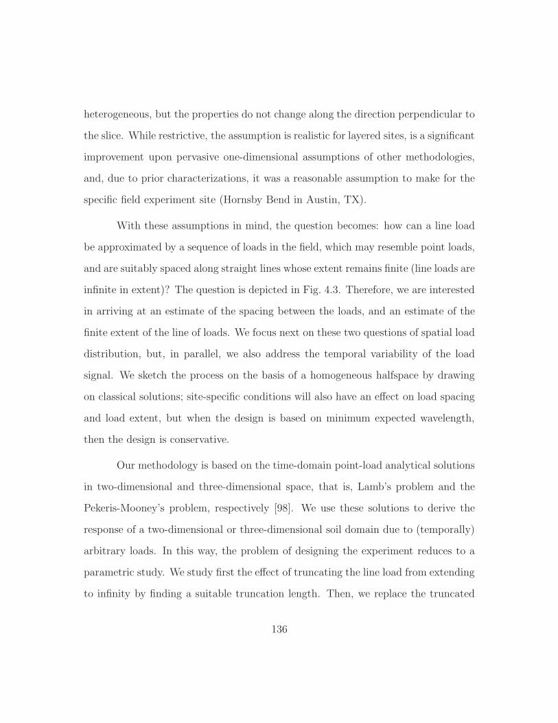
heterogeneous, but the properties do not change along the direction perpendicular to
the slice. While restrictive, the assumption is realistic for layered sites, is a significant
improvement upon pervasive one-dimensional assumptions of other methodologies,
and, due to prior characterizations, it was a reasonable assumption to make for the
specific field experiment site (Hornsby Bend in Austin, TX).
With these assumptions in mind, the question becomes: how can a line load
be approximated by a sequence of loads in the field, which may resemble point loads,
and are suitably spaced along straight lines whose extent remains finite (line loads are
infinite in extent)? The question is depicted in Fig. 4.3. Therefore, we are interested
in arriving at an estimate of the spacing between the loads, and an estimate of the
finite extent of the line of loads. We focus next on these two questions of spatial load
distribution, but, in parallel, we also address the temporal variability of the load
signal. We sketch the process on the basis of a homogeneous halfspace by drawing
on classical solutions; site-specific conditions will also have an effect on load spacing
and load extent, but when the design is based on minimum expected wavelength,
then the design is conservative.
Our methodology is based on the time-domain point-load analytical solutions
in two-dimensional and three-dimensional space, that is, Lamb’s problem and the
Pekeris-Mooney’s problem, respectively [98]. We use these solutions to derive the
response of a two-dimensional or three-dimensional soil domain due to (temporally)
arbitrary loads. In this way, the problem of designing the experiment reduces to a
parametric study. We study first the effect of truncating the line load from extending
to infinity by finding a suitable truncation length. Then, we replace the truncated
136
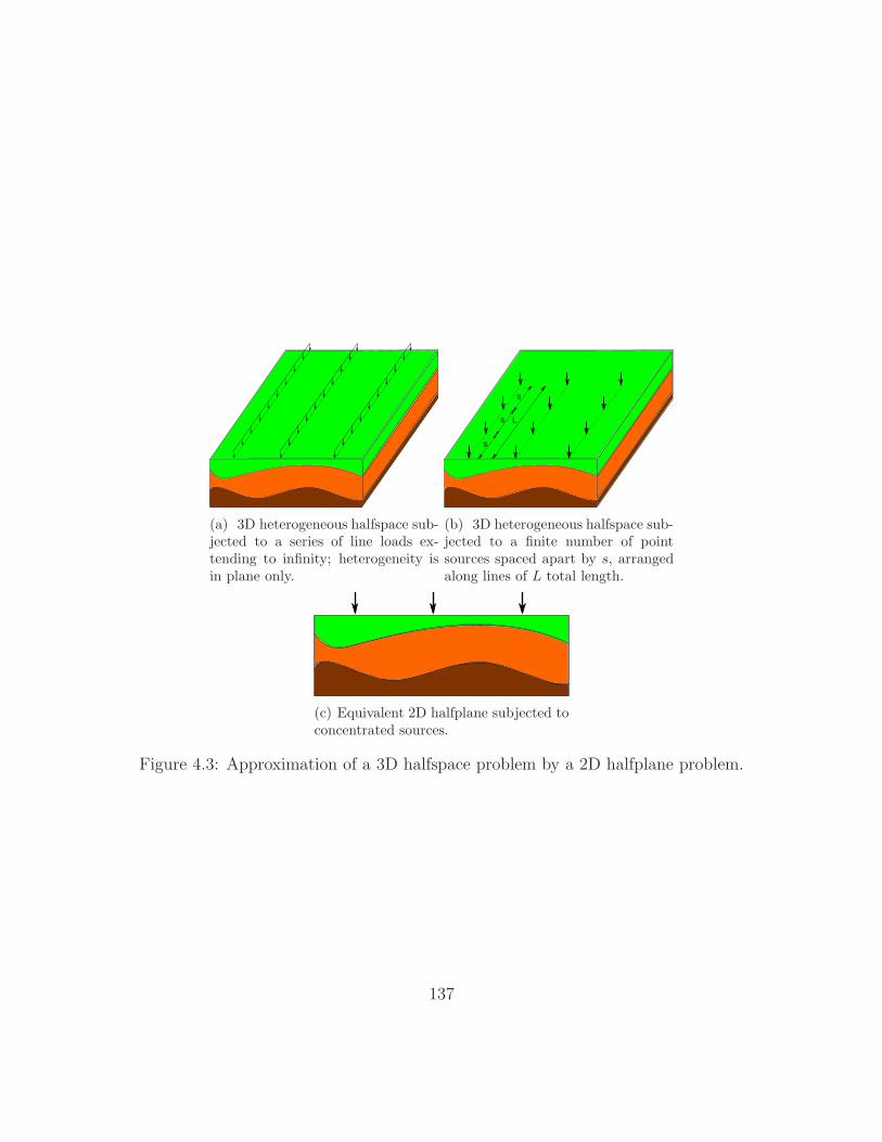
(a) 3D heterogeneous halfspace sub-jected to a series of line loads ex-tending to infinity; heterogeneity isin plane only.
Ls
s
s
(b) 3D heterogeneous halfspace sub-jected to a finite number of pointsources spaced apart by s, arrangedalong lines of L total length.
(c) Equivalent 2D halfplane subjected toconcentrated sources.
Figure 4.3: Approximation of a 3D halfspace problem by a 2D halfplane problem.
137
load line with equivalent point sources and determine the appropriate spacing be-
tween them. Fig. 4.3 displays schematically this objective. Finally, we comment on
designing signals that are appropriate for probing geotechnical sites and also discuss
theoretical and practical issues that arise in such field experiments.
4.2.1 Line load truncation and spacing requirements
An impulsive in-plane point load is applied on the surface of a halfplane and
the resulting displacements are sought. This plane strain problem is equivalent to
an infinite line load applied on the surface of a halfspace. We denote the vertical
displacement of a point (x1, 0) at time t by G2D(x1, t) , where G2D stands for the
Green’s function, and the impulse load acts at the origin. The temporal dependence
of the load can be described via the Dirac-delta function: exploiting superposition,
we obtain the response due to any arbitrary time signal, denoted by f 2D(t), via the
following convolution integral:
u2D(x1, t) =
∫ t
0
f 2D(τ) G2D(x1, t− τ) dτ. (4.21)
The above relation allows us to compute the response of a halfplane subjected to
any temporally arbitrary vertical force that acts on its surface. Special care must be
taken when computing the integral since it has a singularity due to the arrival of the
Rayleigh wave. Therefore, the integral should be interpreted in the Cauchy principal
value sense. Details of the Green’s function G2D(x1, t) can be found in [98].
A vertical point source that varies as a step function in time is applied on
the surface of a halfspace. The vertical displacement of a point (x1, x2, 0) at time t
138
is denoted by G3D(x1, x2, t), and the load acts at the origin. Details of the Green’s
function G3D are given in Appendix F. The time signal can be described via a
Heaviside function. However, we are interested in obtaining the response due to
any arbitrary load, not only those with a simple step-like signature. Hence, our
first attempt in making this problem fit into our needs, is to represent any arbitrary
load f 3D(t) as a summation of Heaviside functions and denote this approximation
by f 3Dn (t). Indeed, given n+ 1 pairs ti, fi = f 3D(ti), i = 0, 1, · · · , n, we have
f 3Dn (t) =
1
2(f0 + f1)(H0 −H1) +
1
2(f1 + f2)(H1 −H2) + · · ·
+1
2(fn−1 + fn)(Hn−1 −Hn), (4.22)
where we used Hi ≡ H(t− ti) for notational simplicity, and ti indicates time value at
node i. Re-arranging the above relation yields the following more convenient form:
f 3Dn (t) =
n∑
i=0
hi H(t− ti), (4.23)
where
hi =
12(f0 + f1), for i = 0,−1
2(fn−1 + fn), for i = n,
12(fi+1 − fi−1), otherwise.
(4.24)
Next, we consider a uniform distribution of point sources, with a Heaviside
time signature, along a line of finite length. Without loss of generality, we assume
that the sources are positioned symmetrically about the origin, and occupy a total
139
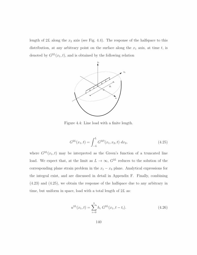
length of 2L along the x2 axis (see Fig. 4.4). The response of the halfspace to this
distribution, at any arbitrary point on the surface along the x1 axis, at time t, is
denoted by G2L(x1, t), and is obtained by the following relation
x1
x2
x3
2L
Figure 4.4: Line load with a finite length.
G2L(x1, t) =
∫ L
−L
G3D(x1, x2, t) dx2, (4.25)
where G2L(x1, t) may be interpreted as the Green’s function of a truncated line
load. We expect that, at the limit as L → ∞, G2L reduces to the solution of the
corresponding plane strain problem in the x1 − x3 plane. Analytical expressions for
the integral exist, and are discussed in detail in Appendix F. Finally, combining
(4.23) and (4.25), we obtain the response of the halfspace due to any arbitrary in
time, but uniform in space, load with a total length of 2L as:
u2L(x1, t) =
n∑
i=0
hi G2L(x1, t− ti). (4.26)
140
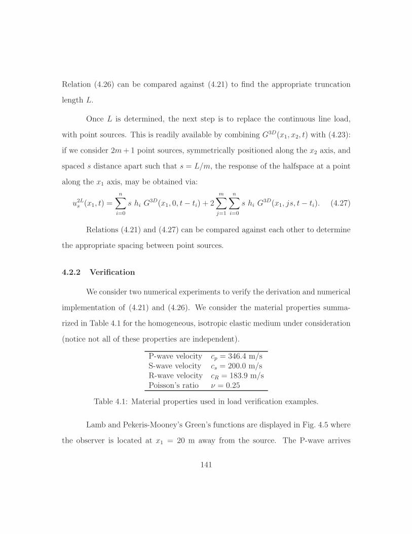
Relation (4.26) can be compared against (4.21) to find the appropriate truncation
length L.
Once L is determined, the next step is to replace the continuous line load,
with point sources. This is readily available by combining G3D(x1, x2, t) with (4.23):
if we consider 2m+1 point sources, symmetrically positioned along the x2 axis, and
spaced s distance apart such that s = L/m, the response of the halfspace at a point
along the x1 axis, may be obtained via:
u2Ls (x1, t) =
n∑
i=0
s hi G3D(x1, 0, t− ti) + 2
m∑
j=1
n∑
i=0
s hi G3D(x1, js, t− ti). (4.27)
Relations (4.21) and (4.27) can be compared against each other to determine
the appropriate spacing between point sources.
4.2.2 Verification
We consider two numerical experiments to verify the derivation and numerical
implementation of (4.21) and (4.26). We consider the material properties summa-
rized in Table 4.1 for the homogeneous, isotropic elastic medium under consideration
(notice not all of these properties are independent).
P-wave velocity cp = 346.4 m/sS-wave velocity cs = 200.0 m/sR-wave velocity cR = 183.9 m/sPoisson’s ratio ν = 0.25
Table 4.1: Material properties used in load verification examples.
Lamb and Pekeris-Mooney’s Green’s functions are displayed in Fig. 4.5 where
the observer is located at x1 = 20 m away from the source. The P-wave arrives
141
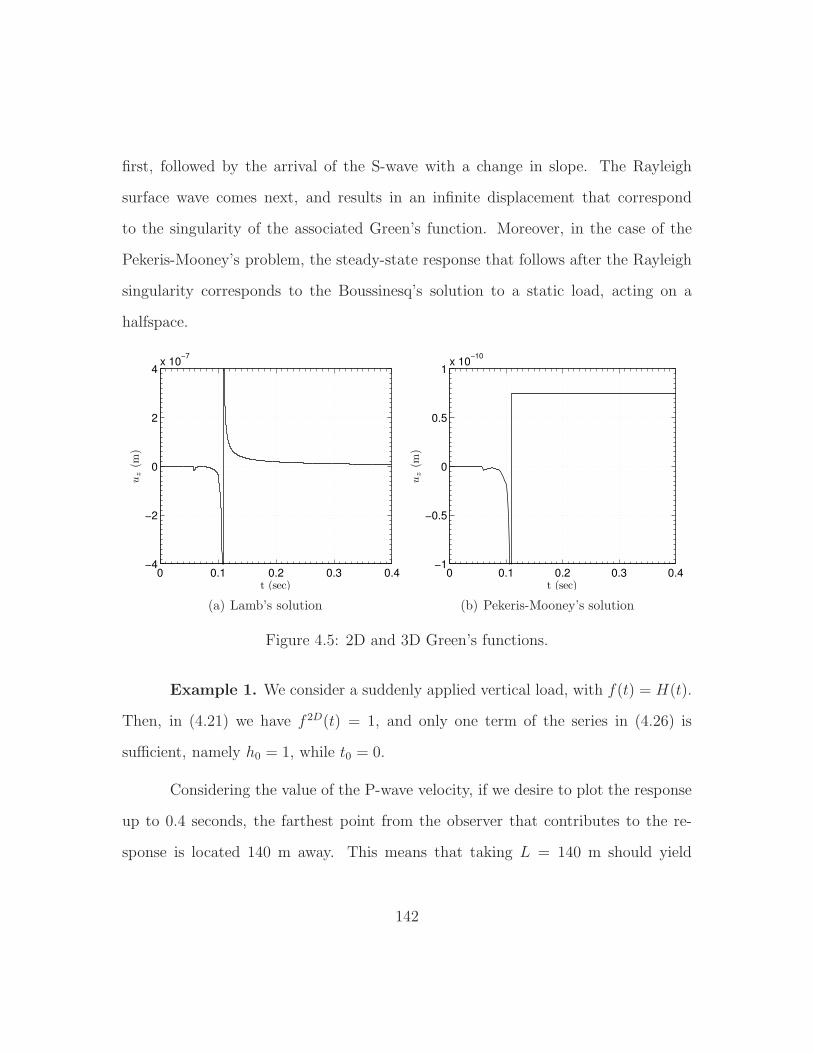
first, followed by the arrival of the S-wave with a change in slope. The Rayleigh
surface wave comes next, and results in an infinite displacement that correspond
to the singularity of the associated Green’s function. Moreover, in the case of the
Pekeris-Mooney’s problem, the steady-state response that follows after the Rayleigh
singularity corresponds to the Boussinesq’s solution to a static load, acting on a
halfspace.
0 0.1 0.2 0.3 0.4−4
−2
0
2
4x 10
−7
t (sec)
uz
(m)
(a) Lamb’s solution
0 0.1 0.2 0.3 0.4−1
−0.5
0
0.5
1x 10
−10
t (sec)
uz
(m)
(b) Pekeris-Mooney’s solution
Figure 4.5: 2D and 3D Green’s functions.
Example 1. We consider a suddenly applied vertical load, with f(t) = H(t).
Then, in (4.21) we have f 2D(t) = 1, and only one term of the series in (4.26) is
sufficient, namely h0 = 1, while t0 = 0.
Considering the value of the P-wave velocity, if we desire to plot the response
up to 0.4 seconds, the farthest point from the observer that contributes to the re-
sponse is located 140 m away. This means that taking L = 140 m should yield
142
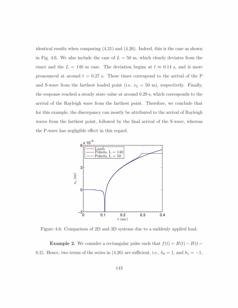
identical results when comparing (4.21) and (4.26). Indeed, this is the case as shown
in Fig. 4.6. We also include the case of L = 50 m, which clearly deviates from the
exact and the L = 140 m case. The deviation begins at t ≈ 0.14 s, and is more
pronounced at around t = 0.27 s. These times correspond to the arrival of the P
and S-wave from the farthest loaded point (i.e. x2 = 50 m), respectively. Finally,
the response reached a steady state value at around 0.29 s, which corresponds to the
arrival of the Rayleigh wave from the farthest point. Therefore, we conclude that
for this example, the discrepancy can mostly be attributed to the arrival of Rayleigh
waves from the farthest point, followed by the final arrival of the S-wave, whereas
the P-wave has negligible effect in this regard.
0 0.1 0.2 0.3 0.4−3
0
3
6x 10
−9
t (sec)
uz
(m)
LambPekeris, L = 140Pekeris, L = 50
Figure 4.6: Comparison of 2D and 3D systems due to a suddenly applied load.
Example 2. We consider a rectangular pulse such that f(t) = H(t)−H(t−
0.2). Hence, two terms of the series in (4.26) are sufficient, i.e., h0 = 1, and h1 = −1,
143
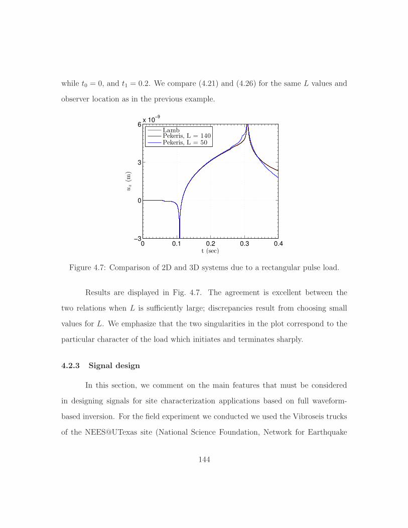
while t0 = 0, and t1 = 0.2. We compare (4.21) and (4.26) for the same L values and
observer location as in the previous example.
0 0.1 0.2 0.3 0.4−3
0
3
6x 10
−9
t (sec)
uz
(m)
LambPekeris, L = 140Pekeris, L = 50
Figure 4.7: Comparison of 2D and 3D systems due to a rectangular pulse load.
Results are displayed in Fig. 4.7. The agreement is excellent between the
two relations when L is sufficiently large; discrepancies result from choosing small
values for L. We emphasize that the two singularities in the plot correspond to the
particular character of the load which initiates and terminates sharply.
4.2.3 Signal design
In this section, we comment on the main features that must be considered
in designing signals for site characterization applications based on full waveform-
based inversion. For the field experiment we conducted we used the Vibroseis trucks
of the NEES@UTexas site (National Science Foundation, Network for Earthquake
144
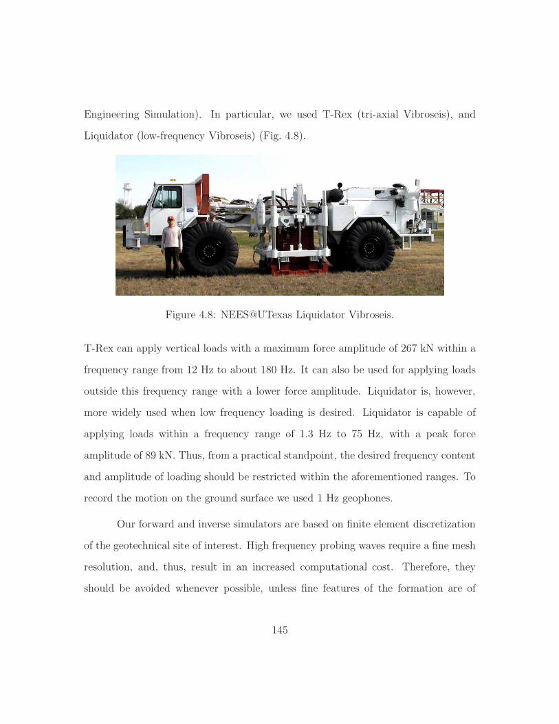
Engineering Simulation). In particular, we used T-Rex (tri-axial Vibroseis), and
Liquidator (low-frequency Vibroseis) (Fig. 4.8).
Figure 4.8: NEES@UTexas Liquidator Vibroseis.
T-Rex can apply vertical loads with a maximum force amplitude of 267 kN within a
frequency range from 12 Hz to about 180 Hz. It can also be used for applying loads
outside this frequency range with a lower force amplitude. Liquidator is, however,
more widely used when low frequency loading is desired. Liquidator is capable of
applying loads within a frequency range of 1.3 Hz to 75 Hz, with a peak force
amplitude of 89 kN. Thus, from a practical standpoint, the desired frequency content
and amplitude of loading should be restricted within the aforementioned ranges. To
record the motion on the ground surface we used 1 Hz geophones.
Our forward and inverse simulators are based on finite element discretization
of the geotechnical site of interest. High frequency probing waves require a fine mesh
resolution, and, thus, result in an increased computational cost. Therefore, they
should be avoided whenever possible, unless fine features of the formation are of
145
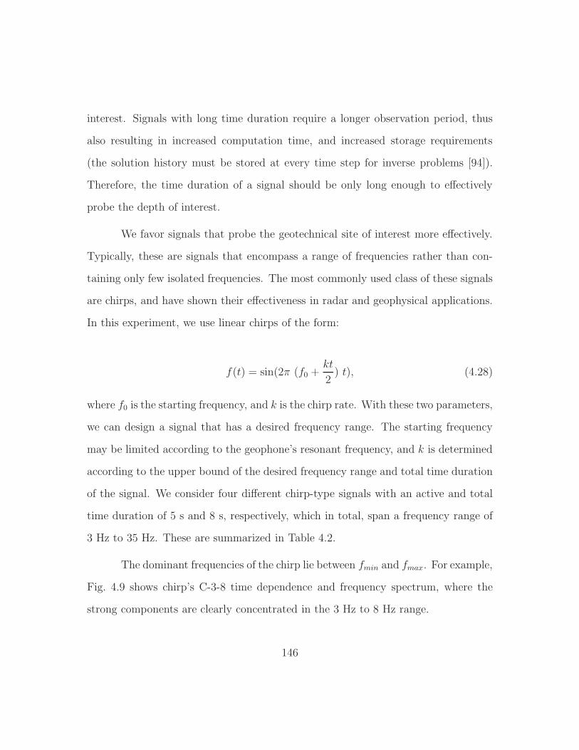
interest. Signals with long time duration require a longer observation period, thus
also resulting in increased computation time, and increased storage requirements
(the solution history must be stored at every time step for inverse problems [94]).
Therefore, the time duration of a signal should be only long enough to effectively
probe the depth of interest.
We favor signals that probe the geotechnical site of interest more effectively.
Typically, these are signals that encompass a range of frequencies rather than con-
taining only few isolated frequencies. The most commonly used class of these signals
are chirps, and have shown their effectiveness in radar and geophysical applications.
In this experiment, we use linear chirps of the form:
f(t) = sin(2π (f0 +kt
2) t), (4.28)
where f0 is the starting frequency, and k is the chirp rate. With these two parameters,
we can design a signal that has a desired frequency range. The starting frequency
may be limited according to the geophone’s resonant frequency, and k is determined
according to the upper bound of the desired frequency range and total time duration
of the signal. We consider four different chirp-type signals with an active and total
time duration of 5 s and 8 s, respectively, which in total, span a frequency range of
3 Hz to 35 Hz. These are summarized in Table 4.2.
The dominant frequencies of the chirp lie between fmin and fmax. For example,
Fig. 4.9 shows chirp’s C-3-8 time dependence and frequency spectrum, where the
strong components are clearly concentrated in the 3 Hz to 8 Hz range.
146
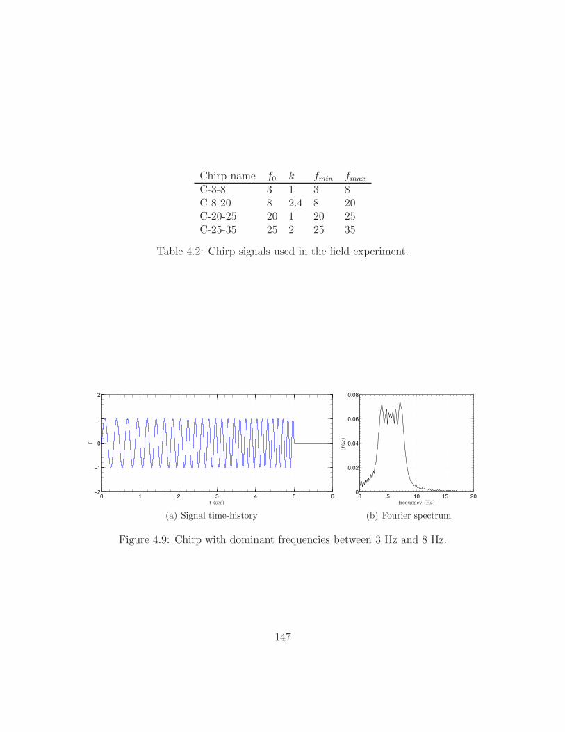
Chirp name f0 k fmin fmax
C-3-8 3 1 3 8C-8-20 8 2.4 8 20C-20-25 20 1 20 25C-25-35 25 2 25 35
Table 4.2: Chirp signals used in the field experiment.
0 1 2 3 4 5 6−2
−1
0
1
2
t (sec)
f
(a) Signal time-history
0 5 10 15 200
0.02
0.04
0.06
0.08
frequency (Hz)
|f(ω
)|
(b) Fourier spectrum
Figure 4.9: Chirp with dominant frequencies between 3 Hz and 8 Hz.
147
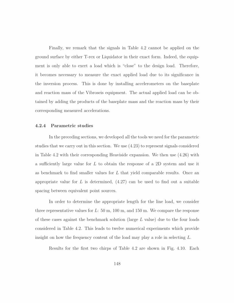
Finally, we remark that the signals in Table 4.2 cannot be applied on the
ground surface by either T-rex or Liquidator in their exact form. Indeed, the equip-
ment is only able to exert a load which is “close” to the design load. Therefore,
it becomes necessary to measure the exact applied load due to its significance in
the inversion process. This is done by installing accelerometers on the baseplate
and reaction mass of the Vibroseis equipment. The actual applied load can be ob-
tained by adding the products of the baseplate mass and the reaction mass by their
corresponding measured accelerations.
4.2.4 Parametric studies
In the preceding sections, we developed all the tools we need for the parametric
studies that we carry out in this section. We use (4.23) to represent signals considered
in Table 4.2 with their corresponding Heaviside expansion. We then use (4.26) with
a sufficiently large value for L to obtain the response of a 2D system and use it
as benchmark to find smaller values for L that yield comparable results. Once an
appropriate value for L is determined, (4.27) can be used to find out a suitable
spacing between equivalent point sources.
In order to determine the appropriate length for the line load, we consider
three representative values for L: 50 m, 100 m, and 150 m. We compare the response
of these cases against the benchmark solution (large L value) due to the four loads
considered in Table 4.2. This leads to twelve numerical experiments which provide
insight on how the frequency content of the load may play a role in selecting L.
Results for the first two chirps of Table 4.2 are shown in Fig. 4.10. Each
148
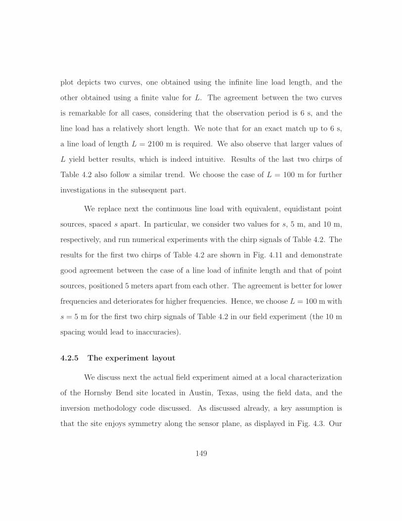
plot depicts two curves, one obtained using the infinite line load length, and the
other obtained using a finite value for L. The agreement between the two curves
is remarkable for all cases, considering that the observation period is 6 s, and the
line load has a relatively short length. We note that for an exact match up to 6 s,
a line load of length L = 2100 m is required. We also observe that larger values of
L yield better results, which is indeed intuitive. Results of the last two chirps of
Table 4.2 also follow a similar trend. We choose the case of L = 100 m for further
investigations in the subsequent part.
We replace next the continuous line load with equivalent, equidistant point
sources, spaced s apart. In particular, we consider two values for s, 5 m, and 10 m,
respectively, and run numerical experiments with the chirp signals of Table 4.2. The
results for the first two chirps of Table 4.2 are shown in Fig. 4.11 and demonstrate
good agreement between the case of a line load of infinite length and that of point
sources, positioned 5 meters apart from each other. The agreement is better for lower
frequencies and deteriorates for higher frequencies. Hence, we choose L = 100 m with
s = 5 m for the first two chirp signals of Table 4.2 in our field experiment (the 10 m
spacing would lead to inaccuracies).
4.2.5 The experiment layout
We discuss next the actual field experiment aimed at a local characterization
of the Hornsby Bend site located in Austin, Texas, using the field data, and the
inversion methodology code discussed. As discussed already, a key assumption is
that the site enjoys symmetry along the sensor plane, as displayed in Fig. 4.3. Our
149
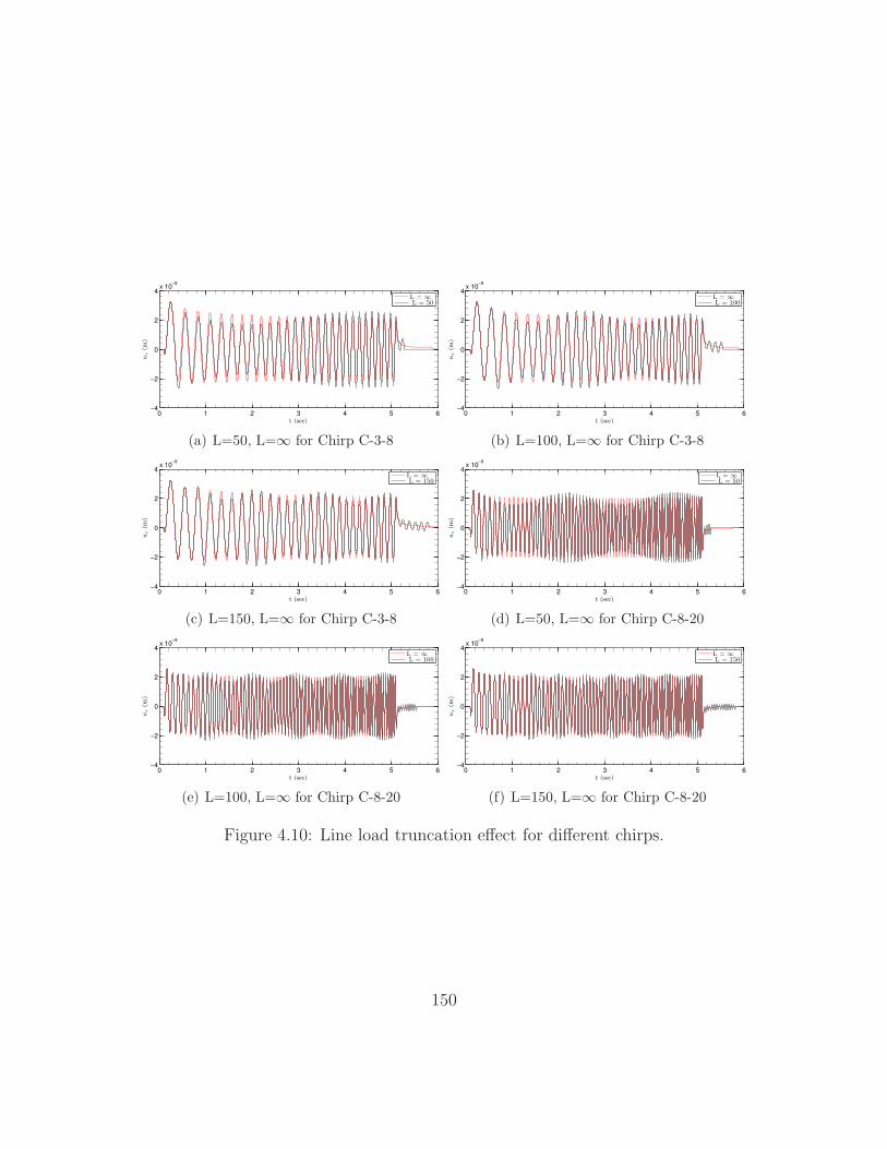
0 1 2 3 4 5 6−4
−2
0
2
4x 10
−9
t (sec)
uz
(m)
L = ∞L = 50
(a) L=50, L=∞ for Chirp C-3-8
0 1 2 3 4 5 6−4
−2
0
2
4x 10
−9
t (sec)
uz
(m)
L = ∞L = 100
(b) L=100, L=∞ for Chirp C-3-8
0 1 2 3 4 5 6−4
−2
0
2
4x 10
−9
t (sec)
uz
(m)
L = ∞L = 150
(c) L=150, L=∞ for Chirp C-3-8
0 1 2 3 4 5 6−4
−2
0
2
4x 10
−9
t (sec)
uz
(m)
L = ∞L = 50
(d) L=50, L=∞ for Chirp C-8-20
0 1 2 3 4 5 6−4
−2
0
2
4x 10
−9
t (sec)
uz
(m)
L = ∞L = 100
(e) L=100, L=∞ for Chirp C-8-20
0 1 2 3 4 5 6−4
−2
0
2
4x 10
−9
t (sec)
uz
(m)
L = ∞L = 150
(f) L=150, L=∞ for Chirp C-8-20
Figure 4.10: Line load truncation effect for different chirps.
150
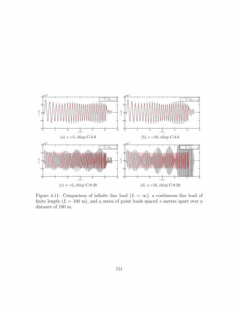
0 1 2 3 4 5 6−4
−2
0
2
4x 10
−9
t (sec)
uz
(m)
L = ∞L = 100, s = 5
(a) s =5, chirp C-3-8
0 1 2 3 4 5 6−4
−2
0
2
4x 10
−9
t (sec)
uz
(m)
L = ∞L = 100, s = 10
(b) s =10, chirp C-3-8
0 1 2 3 4 5 6−4
−2
0
2
4x 10
−9
t (sec)
uz
(m)
L = ∞L = 100, s = 5
(c) s =5, chirp C-8-20
0 1 2 3 4 5 6−4
−2
0
2
4x 10
−9
t (sec)
uz
(m)
L = ∞L = 100, s = 10
(d) s =10, chirp C-8-20
Figure 4.11: Comparison of infinite line load (L = ∞), a continuous line load offinite length (L = 100 m), and a series of point loads spaced s meters apart over adistance of 100 m.
151

objective is to explore a site of length 200 m along this plane. We place sensors every
5 m. These are shown in Fig. 4.12 with bullets. We consider sources, also spaced
5 m apart from each other, indicated by squares, which are placed along five lines of
length 100 m. Due to the symmetry assumptions, we consider sources only on one
side of the sensor plane, and assume that if we had sources on the mirror side, they
would have yielded the same response as their existing counterparts. The experiment
was performed in Austin, TX, Hornsby Bend in October 2010 (Fig. 4.13).
source locationsensor location
x1,ξ 1
x2,ξ 2
(x1,x 2) (ξ1,ξ 2)
10
0 m
200 m
5 m
5 m
Figure 4.12: The field experiment layout.
4.3 Field experiment records and data processing
In this section, we discuss a subset of the field recorded data, and outline the
data processing procedure. The latter consists of two main parts. First, identifica-
tion and reduction of noise effects associated with the recorded data, and, secondly,
integrating the data in such a way that they readily fit the requirements of our
152
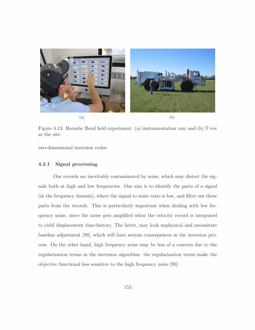
(a) (b)
Figure 4.13: Hornsby Bend field experiment: (a) instrumentation van; and (b) T-rexat the site.
two-dimensional inversion codes.
4.3.1 Signal processing
Our records are inevitably contaminated by noise, which may distort the sig-
nals both at high and low frequencies. Our aim is to identify the parts of a signal
(in the frequency domain), where the signal to noise ratio is low, and filter out these
parts from the records. This is particularly important when dealing with low fre-
quency noise, since the noise gets amplified when the velocity record is integrated
to yield displacement time-history. The latter, may look unphysical and necessitate
baseline adjustment [99], which will have serious consequences in the inversion pro-
cess. On the other hand, high frequency noise may be less of a concern due to the
regularization terms in the inversion algorithm: the regularization terms make the
objective functional less sensitive to the high frequency noise [93].
153
A sampling frequency of 820 Hz is used for digital data collection. Assuming
the highly unlikely event that data being contaminated by noise up to a range of
100 Hz (noise was observed up to 70 Hz), a sampling rate of 200 Hz could prevent
aliasing effects according to the Nyquist sampling theorem [100]. In this sense, we
oversampled the data, which causes no harm. Moreover, in order to reduce the effects
of ambient noise, we repeated each loading five times, and use the average in our
analysis.
We favor finite-impulse-response (FIR) filters since they preserve a signal’s
phase information (linear phase), and do not result in phase distortion, as commonly
occurs in more popular infinite-impulse-response (IIR) filters [100]. We use Matlab’s
equiripple bandpass filter, with high and low cuts of 2.5 Hz and 12 Hz, respectively,
and high and low slopes of 60 dB/octave and 38 db/octave, for the C-3-8 chirp (see
Table 4.2). For the C-8-20 chirp, we use the same type of filter, with high and low
cuts of 2.5 Hz and 25 Hz, and high and low slopes of 60 dB/octave and 26 db/octave,
respectively.
Next, we present some of the field experiment records both in their unpro-
cessed and processed form. For example, Fig. 4.14 shows the C-3-8 chirp, applied
by Liquidator at (ξ1, ξ2) = (0, 0). The record may be compared with the record
in Fig. 4.9, which is the corresponding theoretical curve. Notice that the applied
load lies mainly within the design frequency range, except for the relatively small-
component high-frequency noise, which probably originates with the Liquidator’s
engine and hydraulics.
Figures 4.15, 4.16, and 4.17 depict a subset of the recorded sensor data: both
154
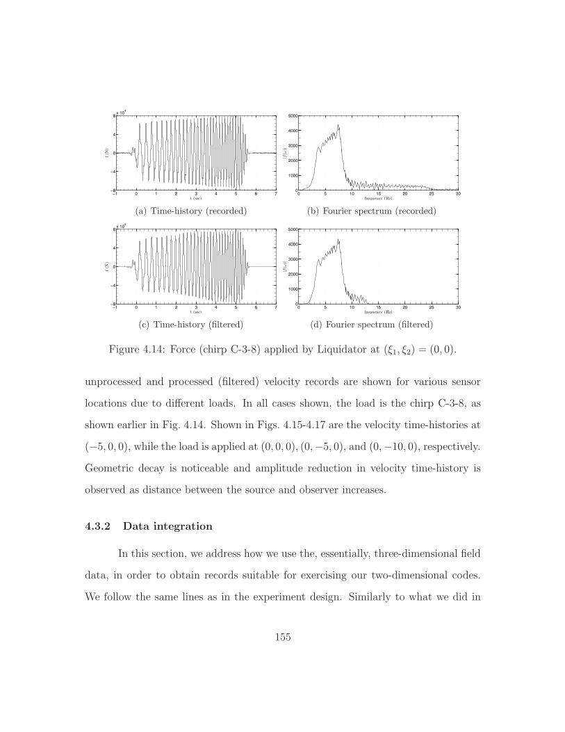
−1 0 1 2 3 4 5 6 7−8
−4
0
4
8x 10
4
t (sec)
f(N
)
(a) Time-history (recorded)
0 5 10 15 20 25 300
1000
2000
3000
4000
5000
frequency (Hz)
|f(ω
)|
(b) Fourier spectrum (recorded)
−1 0 1 2 3 4 5 6 7−8
−4
0
4
8x 10
4
t (sec)
f(N
)
(c) Time-history (filtered)
0 5 10 15 20 25 300
1000
2000
3000
4000
5000
frequency (Hz)
|f(ω
)|
(d) Fourier spectrum (filtered)
Figure 4.14: Force (chirp C-3-8) applied by Liquidator at (ξ1, ξ2) = (0, 0).
unprocessed and processed (filtered) velocity records are shown for various sensor
locations due to different loads. In all cases shown, the load is the chirp C-3-8, as
shown earlier in Fig. 4.14. Shown in Figs. 4.15-4.17 are the velocity time-histories at
(−5, 0, 0), while the load is applied at (0, 0, 0), (0,−5, 0), and (0,−10, 0), respectively.
Geometric decay is noticeable and amplitude reduction in velocity time-history is
observed as distance between the source and observer increases.
4.3.2 Data integration
In this section, we address how we use the, essentially, three-dimensional field
data, in order to obtain records suitable for exercising our two-dimensional codes.
We follow the same lines as in the experiment design. Similarly to what we did in
155
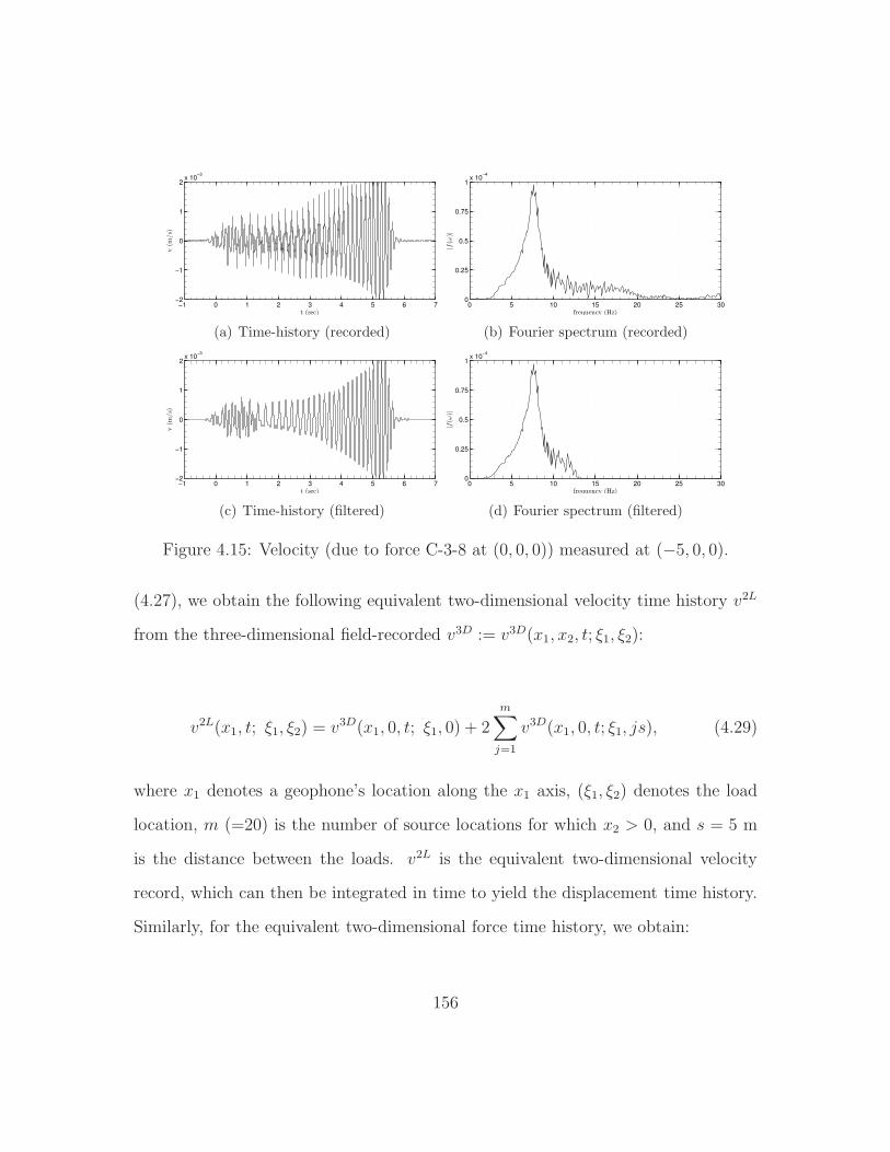
−1 0 1 2 3 4 5 6 7−2
−1
0
1
2x 10
−3
t (sec)
v(m
/s)
(a) Time-history (recorded)
0 5 10 15 20 25 300
0.25
0.5
0.75
1x 10
−4
frequency (Hz)
|f(ω
)|
(b) Fourier spectrum (recorded)
−1 0 1 2 3 4 5 6 7−2
−1
0
1
2x 10
−3
t (sec)
v(m
/s)
(c) Time-history (filtered)
0 5 10 15 20 25 300
0.25
0.5
0.75
1x 10
−4
frequency (Hz)
|f(ω
)|
(d) Fourier spectrum (filtered)
Figure 4.15: Velocity (due to force C-3-8 at (0, 0, 0)) measured at (−5, 0, 0).
(4.27), we obtain the following equivalent two-dimensional velocity time history v2L
from the three-dimensional field-recorded v3D := v3D(x1, x2, t; ξ1, ξ2):
v2L(x1, t; ξ1, ξ2) = v3D(x1, 0, t; ξ1, 0) + 2m∑
j=1
v3D(x1, 0, t; ξ1, js), (4.29)
where x1 denotes a geophone’s location along the x1 axis, (ξ1, ξ2) denotes the load
location, m (=20) is the number of source locations for which x2 > 0, and s = 5 m
is the distance between the loads. v2L is the equivalent two-dimensional velocity
record, which can then be integrated in time to yield the displacement time history.
Similarly, for the equivalent two-dimensional force time history, we obtain:
156
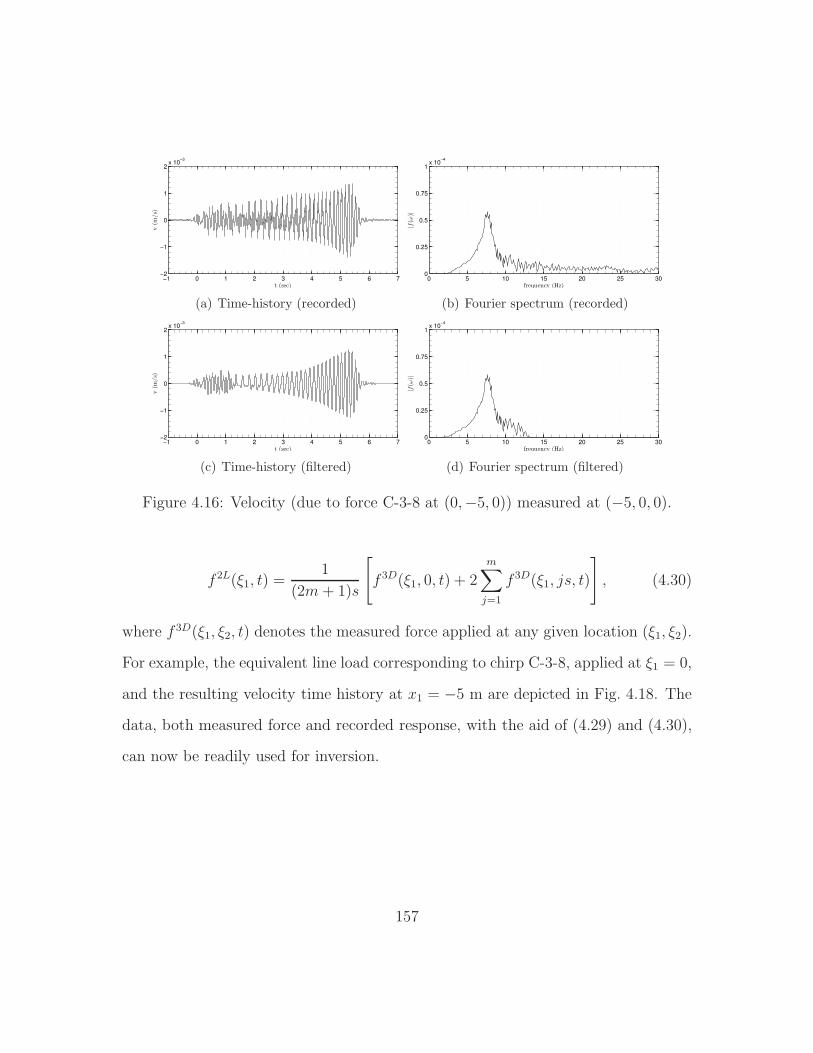
−1 0 1 2 3 4 5 6 7−2
−1
0
1
2x 10
−3
t (sec)
v(m
/s)
(a) Time-history (recorded)
0 5 10 15 20 25 300
0.25
0.5
0.75
1x 10
−4
frequency (Hz)
|f(ω
)|
(b) Fourier spectrum (recorded)
−1 0 1 2 3 4 5 6 7−2
−1
0
1
2x 10
−3
t (sec)
v(m
/s)
(c) Time-history (filtered)
0 5 10 15 20 25 300
0.25
0.5
0.75
1x 10
−4
frequency (Hz)
|f(ω
)|
(d) Fourier spectrum (filtered)
Figure 4.16: Velocity (due to force C-3-8 at (0,−5, 0)) measured at (−5, 0, 0).
f 2L(ξ1, t) =1
(2m+ 1)s
[f 3D(ξ1, 0, t) + 2
m∑
j=1
f 3D(ξ1, js, t)
], (4.30)
where f 3D(ξ1, ξ2, t) denotes the measured force applied at any given location (ξ1, ξ2).
For example, the equivalent line load corresponding to chirp C-3-8, applied at ξ1 = 0,
and the resulting velocity time history at x1 = −5 m are depicted in Fig. 4.18. The
data, both measured force and recorded response, with the aid of (4.29) and (4.30),
can now be readily used for inversion.
157
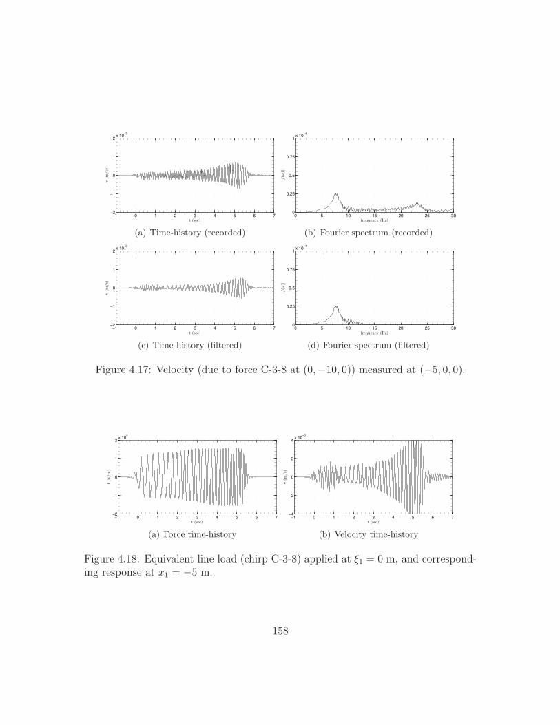
−1 0 1 2 3 4 5 6 7−2
−1
0
1
2x 10
−3
t (sec)
v(m
/s)
(a) Time-history (recorded)
0 5 10 15 20 25 300
0.25
0.5
0.75
1x 10
−4
frequency (Hz)
|f(ω
)|
(b) Fourier spectrum (recorded)
−1 0 1 2 3 4 5 6 7−2
−1
0
1
2x 10
−3
t (sec)
v(m
/s)
(c) Time-history (filtered)
0 5 10 15 20 25 300
0.25
0.5
0.75
1x 10
−4
frequency (Hz)
|f(ω
)|
(d) Fourier spectrum (filtered)
Figure 4.17: Velocity (due to force C-3-8 at (0,−10, 0)) measured at (−5, 0, 0).
−1 0 1 2 3 4 5 6 7−2
−1
0
1
2x 10
4
t (sec)
f(N
/m
)
(a) Force time-history
−1 0 1 2 3 4 5 6 7−4
−2
0
2
4x 10
−3
t (sec)
v(m
/s)
(b) Velocity time-history
Figure 4.18: Equivalent line load (chirp C-3-8) applied at ξ1 = 0 m, and correspond-ing response at x1 = −5 m.
158
4.4 Inversion results using field experiment data
In this section, we use the inversion theory discussed earlier, along with mea-
sured data from the field experiment, to arrive at an estimate of the spatial distri-
bution of the P and S wave velocities at the target site (Hornsby Bend).
The target domain is a two-dimensional slice, 200 m wide and 48 m deep.
The domain is surrounded on its sides and bottom by a 10 m-thick PML to absorb
outgoing waves. We use bilinear quadrilateral elements with element size of 1 m
when applying the C-3-8 chirp (see Table 4.2), whereas 8-noded serendipity elements
of the same size are used for higher frequency chirps. In all cases, we use 1 m × 1 m
bilinear quadrilateral elements to interpolate the material properties.
According to the experiment layout in Fig. 4.12, we apply loads at every 5 m
along five lines. T-Rex was used for loading along the lines x1 = −60 m, +30 m,
and +60 m, whereas Liquidator was used to load along x1 = −30 m, and 0 m. We
used 36 geophones with a resonant frequency of 1 Hz at every 5 m, along the x1 axis.
After processing the recorded data, per the discussion of the preceding section, we
proceeded with the inversion process.
4.4.1 Inversion process
The inversion process begins with an initial profile for both of the Lame
parameters (linear in depth or homogeneous), and iteratively updates the profile until
the misfit between the measured response and the computed response obtained at
each inversion iteration is minimized. The convergence rate of the inversion process
to the target profile, and even the success of the process itself, depends greatly
159
on the initial guess, as is typically the case. An initial profile, which is close to the
target profile, will likely need fewer number of iterations to converge, compared to an
arbitrary initial profile. This fact can be exploited to speed up the convergence. If, for
example, during a field experiment, an SASW experiment is performed in addition
to the data collection for the full waveform inversion approach, then the SASW-
rendered profile could be used as initial guess for the full waveform inversion. The
SASW profile will be, by definition, horizontally layered, whereas the full waveform-
based inverted profile will be, in general, arbitrarily heterogeneous.
We start the inversion process by applying the first (measured) equivalent
force corresponding to chirp C-3-8 (see Table 4.2 for the theoretical curve and
Fig. 4.18 for the actual, equivalent measured force). There are 5 loads at our dis-
posal, and 36 measuring locations for every load. Owing to linearity, we apply all 5
loads simultaneously and add their corresponding responses at every sensor location.
Other possibilities for combining the loads also exist [101, 102].
Due to the very construction of the chirp signals, their frequency increases
linearly with time. This may be exploited to further regularize the inversion process,
i.e., we start the inversion process by considering only a portion of the total chirp
duration, arrive at an inverted profile, use the inverted profile as an initial guess to
the next round of inversion, where we increase the duration of the same chirp signal,
thus, gradually, bringing additional frequencies to bear on the inversion process (a,
so-called, continuation scheme). For example, for the site under study, we start with
the first 2 s of the signals, and progressively move up to 7 s duration, in increments
of 1 s. A similar idea was discussed in [58, 103].
160
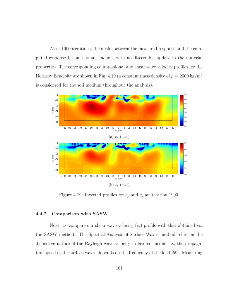
After 1900 iterations, the misfit between the measured response and the com-
puted response becomes small enough, with no discernible update in the material
properties. The corresponding compressional and shear wave velocity profiles for the
Hornsby Bend site are shown in Fig. 4.19 (a constant mass density of ρ = 2000 kg/m3
is considered for the soil medium throughout the analysis).
x1 (m)
x3
(m)
−100 −90 −80 −70 −60 −50 −40 −30 −20 −10 0 10 20 30 40 50 60 70 80 90 100
−50
−40
−30
−20
−10
0
200
300
400
500
600
700
800
900
(a) cp (m/s)
x1 (m)
x3
(m)
−100 −90 −80 −70 −60 −50 −40 −30 −20 −10 0 10 20 30 40 50 60 70 80 90 100
−50
−40
−30
−20
−10
0
100
200
300
400
500
600
(b) cs (m/s)
Figure 4.19: Inverted profiles for cp and cs at iteration 1900.
4.4.2 Comparison with SASW
Next, we compare our shear wave velocity (cs) profile with that obtained via
the SASW method. The Spectral-Analysis-of-Surface-Waves method relies on the
dispersive nature of the Rayleigh wave velocity in layered media, i.e., the propaga-
tion speed of the surface waves depends on the frequency of the load [59]. Measuring
161
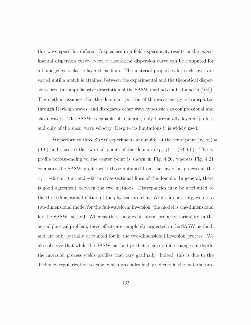
this wave speed for different frequencies in a field experiment, results in the exper-
imental dispersion curve. Next, a theoretical dispersion curve can be computed for
a homogeneous elastic layered medium. The material properties for each layer are
varied until a match is attained between the experimental and the theoretical disper-
sion curve (a comprehensive description of the SASW method can be found in [104]).
The method assumes that the dominant portion of the wave energy is transported
through Rayleigh waves, and disregards other wave types such as compressional and
shear waves. The SASW is capable of rendering only horizontally layered profiles
and only of the shear wave velocity. Despite its limitations it is widely used.
We performed three SASW experiments at our site: at the centerpoint (x1, x2) =
(0, 0) and close to the two end points of the domain (x1, x2) = (±90, 0). The cs
profile corresponding to the center point is shown in Fig. 4.20, whereas Fig. 4.21
compares the SASW profile with those obtained from the inversion process at the
x1 = −90 m, 0 m, and +90 m cross-sectional lines of the domain. In general, there
is good agreement between the two methods. Discrepancies may be attributed to
the three-dimensional nature of the physical problem. While in our study, we use a
two-dimensional model for the full-waveform inversion, the model is one-dimensional
for the SASW method. Whereas there may exist lateral property variability in the
actual physical problem, these effects are completely neglected in the SASW method,
and are only partially accounted for in the two-dimensional inversion process. We
also observe that while the SASW method predicts sharp profile changes in depth,
the inversion process yields profiles that vary gradually. Indeed, this is due to the
Tikhonov regularization scheme, which precludes high gradients in the material pro-
162
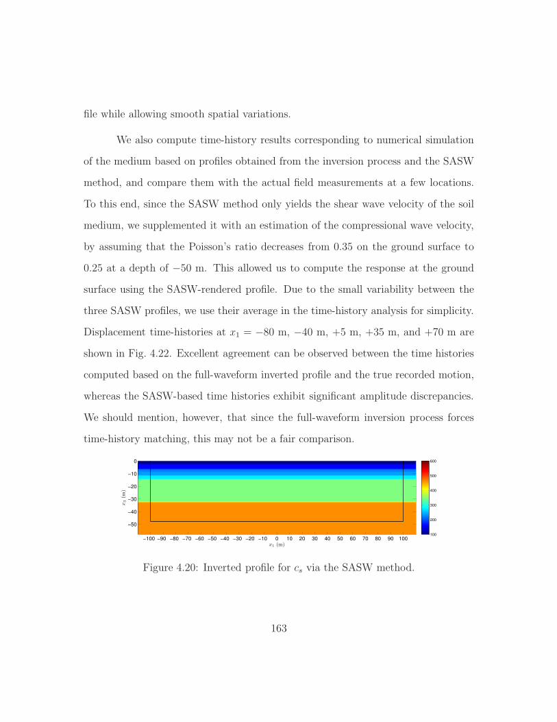
file while allowing smooth spatial variations.
We also compute time-history results corresponding to numerical simulation
of the medium based on profiles obtained from the inversion process and the SASW
method, and compare them with the actual field measurements at a few locations.
To this end, since the SASW method only yields the shear wave velocity of the soil
medium, we supplemented it with an estimation of the compressional wave velocity,
by assuming that the Poisson’s ratio decreases from 0.35 on the ground surface to
0.25 at a depth of −50 m. This allowed us to compute the response at the ground
surface using the SASW-rendered profile. Due to the small variability between the
three SASW profiles, we use their average in the time-history analysis for simplicity.
Displacement time-histories at x1 = −80 m, −40 m, +5 m, +35 m, and +70 m are
shown in Fig. 4.22. Excellent agreement can be observed between the time histories
computed based on the full-waveform inverted profile and the true recorded motion,
whereas the SASW-based time histories exhibit significant amplitude discrepancies.
We should mention, however, that since the full-waveform inversion process forces
time-history matching, this may not be a fair comparison.
x1 (m)
x3
(m)
−100 −90 −80 −70 −60 −50 −40 −30 −20 −10 0 10 20 30 40 50 60 70 80 90 100
−50
−40
−30
−20
−10
0
100
200
300
400
500
600
Figure 4.20: Inverted profile for cs via the SASW method.
163
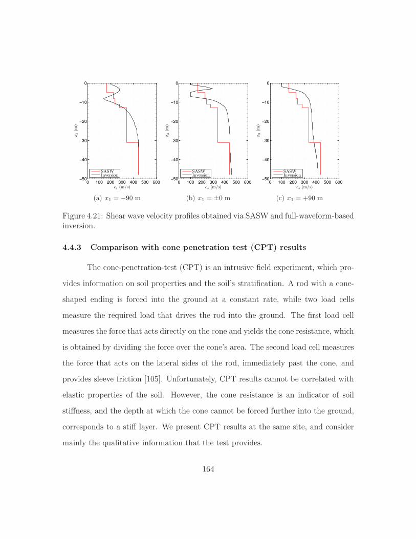
0 100 200 300 400 500 600−50
−40
−30
−20
−10
0
cs (m/s)
x3
(m)
SASWInversion
(a) x1 = −90 m
0 100 200 300 400 500 600−50
−40
−30
−20
−10
0
cs (m/s)
x3
(m)
SASWInversion
(b) x1 = ±0 m
0 100 200 300 400 500 600−50
−40
−30
−20
−10
0
cs (m/s)
x3
(m)
SASWInversion
(c) x1 = +90 m
Figure 4.21: Shear wave velocity profiles obtained via SASW and full-waveform-basedinversion.
4.4.3 Comparison with cone penetration test (CPT) results
The cone-penetration-test (CPT) is an intrusive field experiment, which pro-
vides information on soil properties and the soil’s stratification. A rod with a cone-
shaped ending is forced into the ground at a constant rate, while two load cells
measure the required load that drives the rod into the ground. The first load cell
measures the force that acts directly on the cone and yields the cone resistance, which
is obtained by dividing the force over the cone’s area. The second load cell measures
the force that acts on the lateral sides of the rod, immediately past the cone, and
provides sleeve friction [105]. Unfortunately, CPT results cannot be correlated with
elastic properties of the soil. However, the cone resistance is an indicator of soil
stiffness, and the depth at which the cone cannot be forced further into the ground,
corresponds to a stiff layer. We present CPT results at the same site, and consider
mainly the qualitative information that the test provides.
164
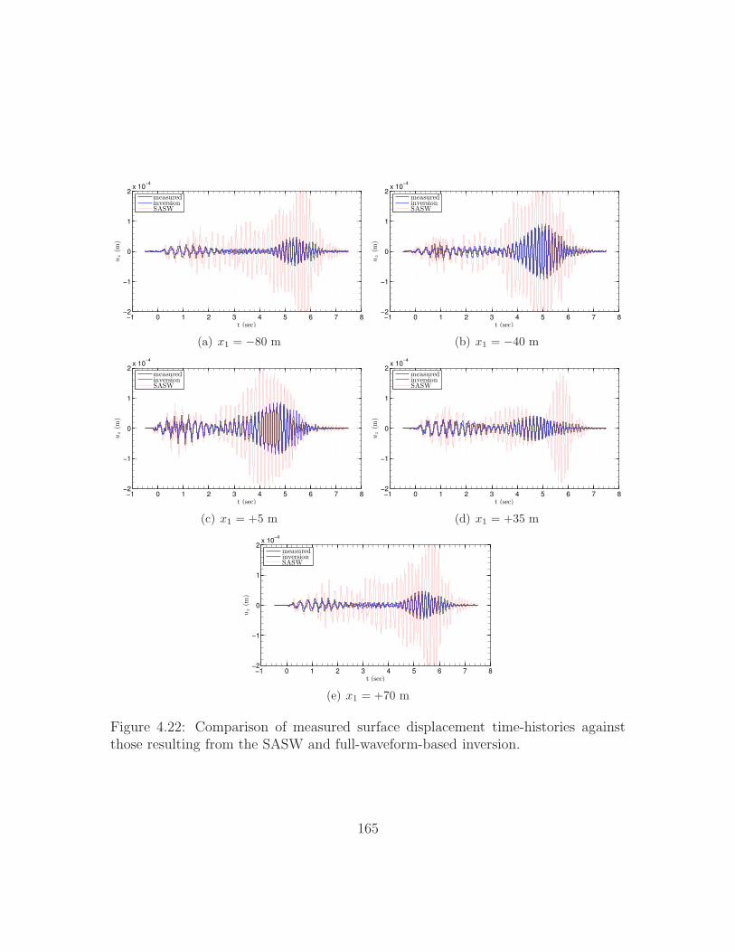
−1 0 1 2 3 4 5 6 7 8−2
−1
0
1
2x 10
−4
t (sec)
uz
(m)
measuredinversionSASW
(a) x1 = −80 m
−1 0 1 2 3 4 5 6 7 8−2
−1
0
1
2x 10
−4
t (sec)
uz
(m)
measuredinversionSASW
(b) x1 = −40 m
−1 0 1 2 3 4 5 6 7 8−2
−1
0
1
2x 10
−4
t (sec)
uz
(m)
measuredinversionSASW
(c) x1 = +5 m
−1 0 1 2 3 4 5 6 7 8−2
−1
0
1
2x 10
−4
t (sec)
uz
(m)
measuredinversionSASW
(d) x1 = +35 m
−1 0 1 2 3 4 5 6 7 8−2
−1
0
1
2x 10
−4
t (sec)
uz
(m)
measuredinversionSASW
(e) x1 = +70 m
Figure 4.22: Comparison of measured surface displacement time-histories againstthose resulting from the SASW and full-waveform-based inversion.
165
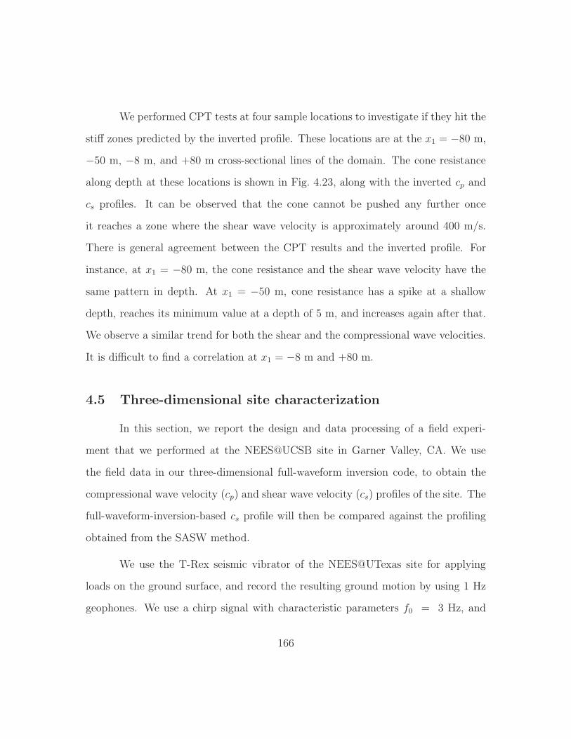
We performed CPT tests at four sample locations to investigate if they hit the
stiff zones predicted by the inverted profile. These locations are at the x1 = −80 m,
−50 m, −8 m, and +80 m cross-sectional lines of the domain. The cone resistance
along depth at these locations is shown in Fig. 4.23, along with the inverted cp and
cs profiles. It can be observed that the cone cannot be pushed any further once
it reaches a zone where the shear wave velocity is approximately around 400 m/s.
There is general agreement between the CPT results and the inverted profile. For
instance, at x1 = −80 m, the cone resistance and the shear wave velocity have the
same pattern in depth. At x1 = −50 m, cone resistance has a spike at a shallow
depth, reaches its minimum value at a depth of 5 m, and increases again after that.
We observe a similar trend for both the shear and the compressional wave velocities.
It is difficult to find a correlation at x1 = −8 m and +80 m.
4.5 Three-dimensional site characterization
In this section, we report the design and data processing of a field experi-
ment that we performed at the NEES@UCSB site in Garner Valley, CA. We use
the field data in our three-dimensional full-waveform inversion code, to obtain the
compressional wave velocity (cp) and shear wave velocity (cs) profiles of the site. The
full-waveform-inversion-based cs profile will then be compared against the profiling
obtained from the SASW method.
We use the T-Rex seismic vibrator of the NEES@UTexas site for applying
loads on the ground surface, and record the resulting ground motion by using 1 Hz
geophones. We use a chirp signal with characteristic parameters f0 = 3 Hz, and
166
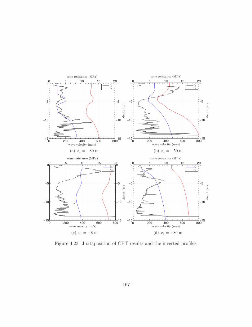
0 200 400 600 800−15
−10
−5
0
wave velocity (m/s)
cscp
0 5 10 15 20
−15
−10
−5
0
cone resistance (MPa)
dep
th(m
)
(a) x1 = −80 m
0 200 400 600 800−15
−10
−5
0
wave velocity (m/s)
cscp
0 5 10 15 20
−15
−10
−5
0
cone resistance (MPa)
dep
th(m
)
(b) x1 = −50 m
0 200 400 600 800−15
−10
−5
0
wave velocity (m/s)
cscp
0 5 10 15 20
−15
−10
−5
0
cone resistance (MPa)
dep
th(m
)
(c) x1 = −8 m
0 200 400 600 800−15
−10
−5
0
wave velocity (m/s)
cscp
0 5 10 15 20
−15
−10
−5
0
cone resistance (MPa)
dep
th(m
)
(d) x1 = +80 m
Figure 4.23: Juxtaposition of CPT results and the inverted profiles.
167

k = 2.8 (see (4.28)), and a total active duration of 2.5 s. This parameterization
results in a loading with dominant frequencies between 3-10 Hz.
4.5.1 The experiment site and layout
The NEES Garner Valley Downhole Array research site in Southern California
is located in a narrow valley, within the Peninsular Ranges batholith, 23 km east of
Hemet, 20 km southwest of Palm Springs, and is just 7 km from the San Jacinto
fault, and 35 km from the San Andreas fault.
We consider a portion of the site of length and width 126 m × 68 m, and
40 m depth. The experiment layout is displayed in Fig. 4.24. The main grid lines
are 10 m apart. The sensors are shown with bullets and sources are indicated by
squares. Overall, we “shake” at 24 locations, and record the site’s response at 63
receiver locations. The experiment was performed on March 13th 2012 (Fig. 4.25).
Figure 4.24: The field experiment layout.
168
(a) (b)
(c) (d)
Figure 4.25: Garner Valley field experiment: (a) T-rex at the site; (b) a buriedgeophone; (c) instrumentation van; and (d) the site.
169
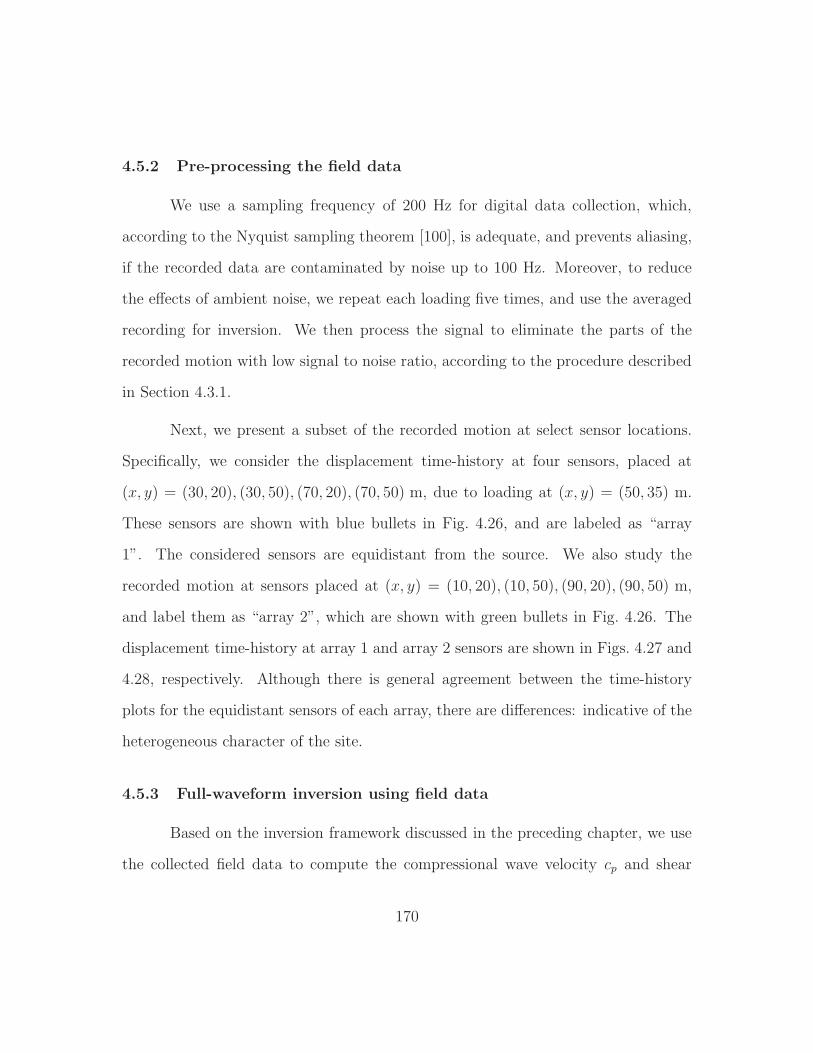
4.5.2 Pre-processing the field data
We use a sampling frequency of 200 Hz for digital data collection, which,
according to the Nyquist sampling theorem [100], is adequate, and prevents aliasing,
if the recorded data are contaminated by noise up to 100 Hz. Moreover, to reduce
the effects of ambient noise, we repeat each loading five times, and use the averaged
recording for inversion. We then process the signal to eliminate the parts of the
recorded motion with low signal to noise ratio, according to the procedure described
in Section 4.3.1.
Next, we present a subset of the recorded motion at select sensor locations.
Specifically, we consider the displacement time-history at four sensors, placed at
(x, y) = (30, 20), (30, 50), (70, 20), (70, 50) m, due to loading at (x, y) = (50, 35) m.
These sensors are shown with blue bullets in Fig. 4.26, and are labeled as “array
1”. The considered sensors are equidistant from the source. We also study the
recorded motion at sensors placed at (x, y) = (10, 20), (10, 50), (90, 20), (90, 50) m,
and label them as “array 2”, which are shown with green bullets in Fig. 4.26. The
displacement time-history at array 1 and array 2 sensors are shown in Figs. 4.27 and
4.28, respectively. Although there is general agreement between the time-history
plots for the equidistant sensors of each array, there are differences: indicative of the
heterogeneous character of the site.
4.5.3 Full-waveform inversion using field data
Based on the inversion framework discussed in the preceding chapter, we use
the collected field data to compute the compressional wave velocity cp and shear
170
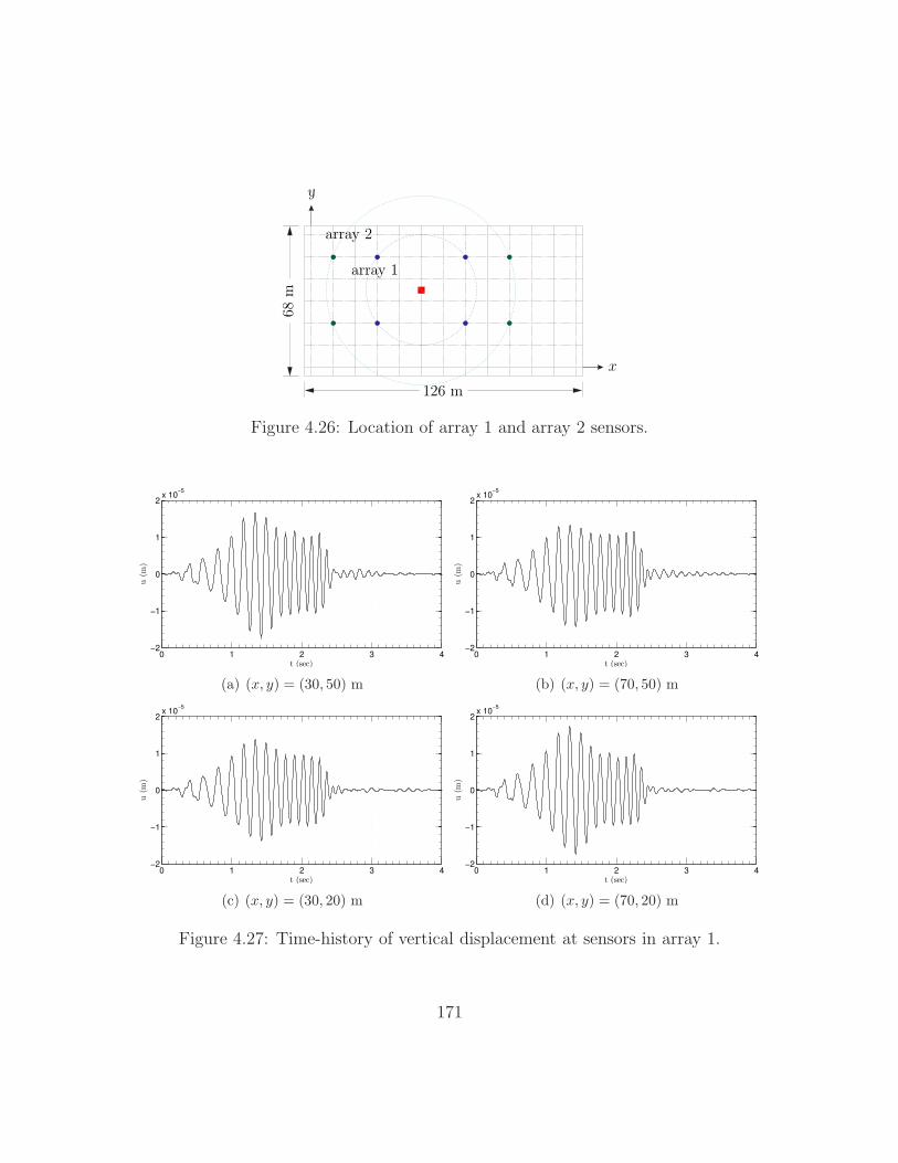
Figure 4.26: Location of array 1 and array 2 sensors.
0 1 2 3 4−2
−1
0
1
2x 10
−5
t (sec)
u(m
)
(a) (x, y) = (30, 50) m
0 1 2 3 4−2
−1
0
1
2x 10
−5
t (sec)
u(m
)
(b) (x, y) = (70, 50) m
0 1 2 3 4−2
−1
0
1
2x 10
−5
t (sec)
u(m
)
(c) (x, y) = (30, 20) m
0 1 2 3 4−2
−1
0
1
2x 10
−5
t (sec)
u(m
)
(d) (x, y) = (70, 20) m
Figure 4.27: Time-history of vertical displacement at sensors in array 1.
171
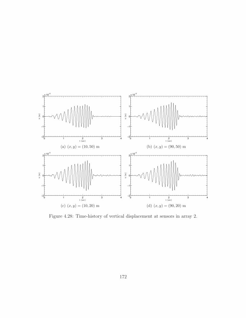
0 1 2 3 4−2
−1
0
1
2x 10
−5
t (sec)
u(m
)
(a) (x, y) = (10, 50) m
0 1 2 3 4−2
−1
0
1
2x 10
−5
t (sec)
u(m
)
(b) (x, y) = (90, 50) m
0 1 2 3 4−2
−1
0
1
2x 10
−5
t (sec)
u(m
)
(c) (x, y) = (10, 20) m
0 1 2 3 4−2
−1
0
1
2x 10
−5
t (sec)
u(m
)
(d) (x, y) = (90, 20) m
Figure 4.28: Time-history of vertical displacement at sensors in array 2.
172
wave velocity cs profiles of the probed site. We consider a cubic (regular) domain
of length, width, and depth 126 × 68 × 40 m. A 10 m-thick PML is placed at the
truncation boundaries. For the PML parameters, we choose αo = 5, βo = 500 s 1,
and a quadratic profile for the attenuation functions, i.e., m = 2. The mass density
is considered to be ρ = 1760 kg/m3 for −2 m ≤ z ≤ 0, ρ = 1880 kg/m3 for
−4 m ≤ z ≤ −2 m, and ρ = 2000 kg/m3 for −40 m ≤ z ≤ −4 m, according to
prior investigations. The material properties at the interfaces ΓI are extended into
the PML. The interior and PML domains are discretized by quadratic hexahedral
spectral elements of size 2 m, and ∆t = 10−3 s. This leads to 3, 885, 648 state
unknowns, and 718, 566 material parameters.
Owing to linearity, we apply all the 24 loads simultaneously, and consider
their superimposed responses at each sensor location. We start the inversion process
with only a portion of the signal, and as the inversion process evolves, we increase the
temporal duration of the signal, thus, progressively introducing higher frequencies,
which allows for profile refinement. We use a smoothed version of the profile obtained
via the SASW method as the starting point of the inversion process.
After 4550 iterations, the misfit between the measured response and the com-
puted response becomes reasonably small, with no strong update in the material
profiles. The corresponding three-dimensional cp and cs profiles for the Garner Val-
ley site are shown in Fig. 4.29, whereas Figs. 4.30-4.32 show the cross-sectional
profiles of the velocity profiles at x = 10, 60, and 90 m. The profiles indicate that
the site under investigation is heterogeneous, revealing the presence of a soft layer
at a depth of about 25 m.
173
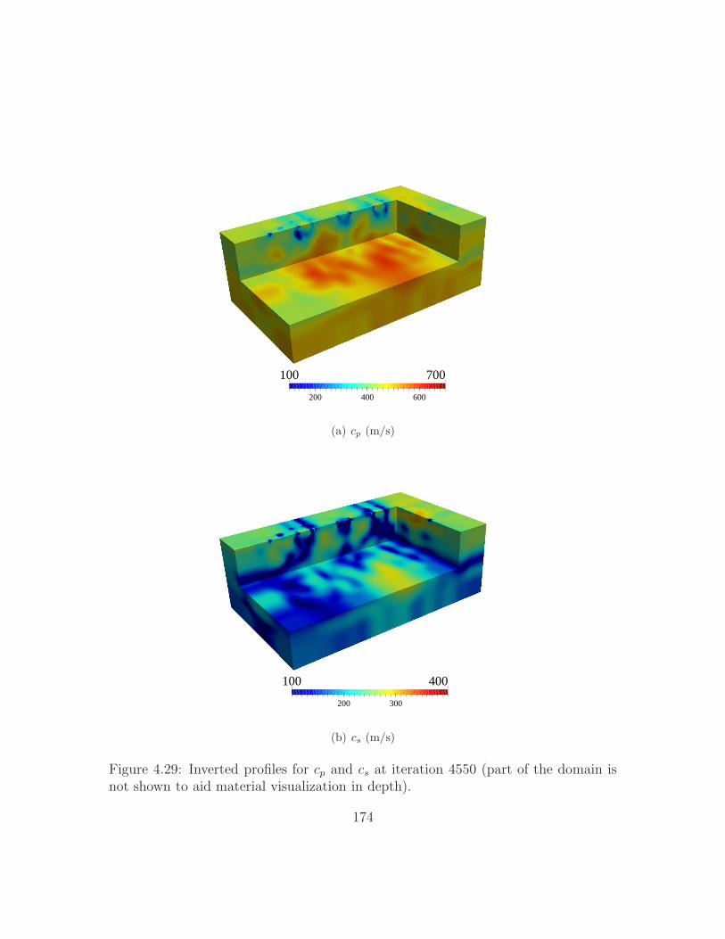
200 400 600
100 700
(a) cp (m/s)
200 300
100 400
(b) cs (m/s)
Figure 4.29: Inverted profiles for cp and cs at iteration 4550 (part of the domain isnot shown to aid material visualization in depth).
174
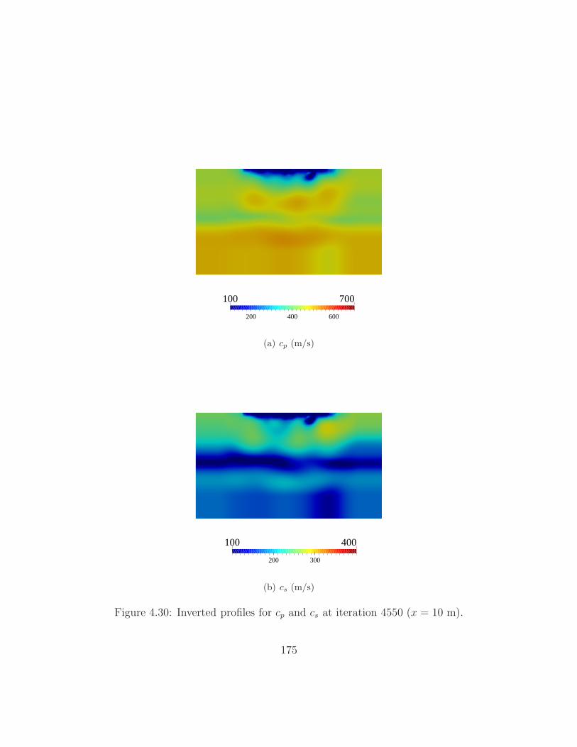
200 400 600
100 700
(a) cp (m/s)
200 300
100 400
(b) cs (m/s)
Figure 4.30: Inverted profiles for cp and cs at iteration 4550 (x = 10 m).
175
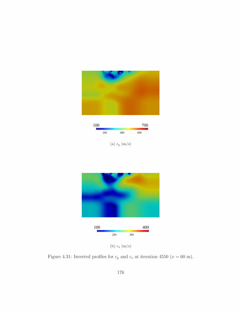
200 400 600
100 700
(a) cp (m/s)
200 300
100 400
(b) cs (m/s)
Figure 4.31: Inverted profiles for cp and cs at iteration 4550 (x = 60 m).
176
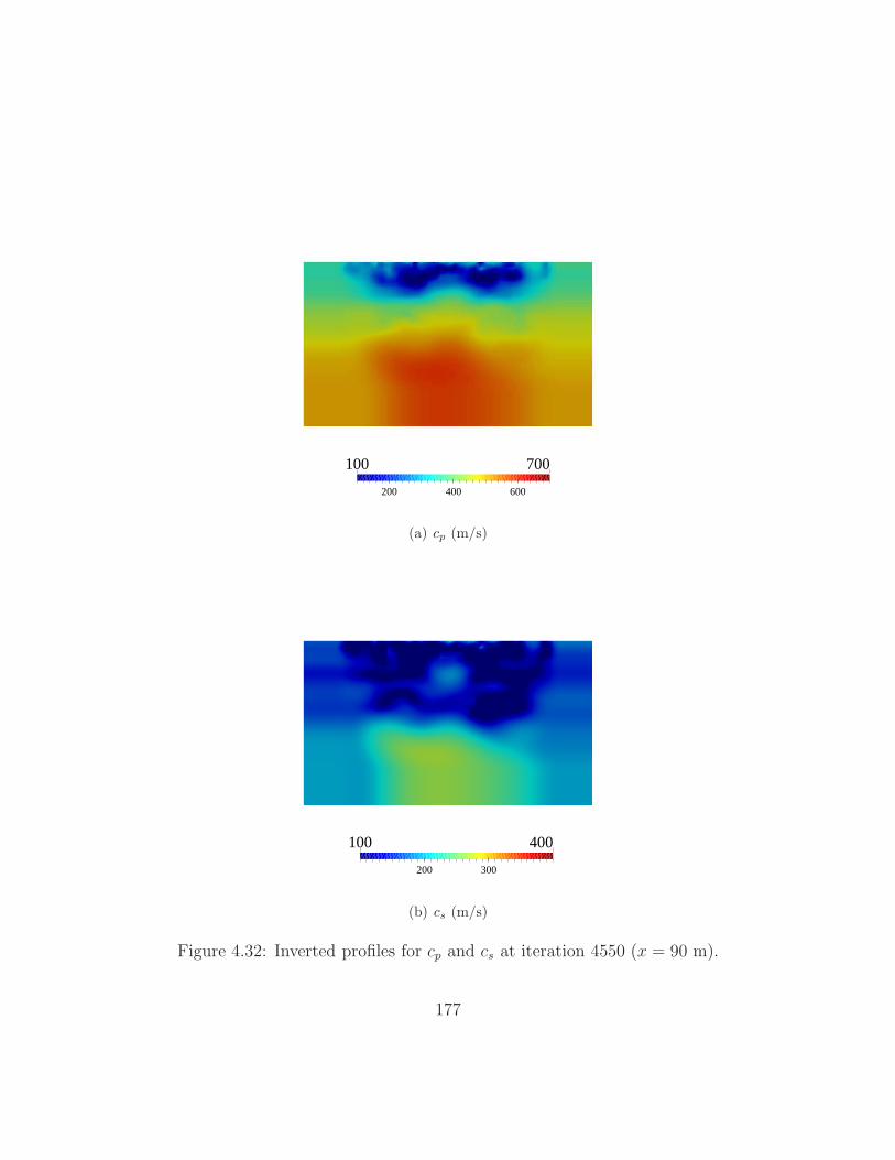
200 400 600
100 700
(a) cp (m/s)
200 300
100 400
(b) cs (m/s)
Figure 4.32: Inverted profiles for cp and cs at iteration 4550 (x = 90 m).
177
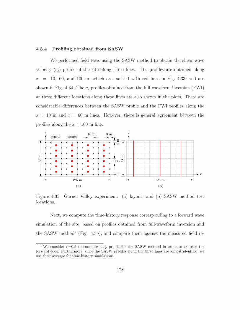
4.5.4 Profiling obtained from SASW
We performed field tests using the SASW method to obtain the shear wave
velocity (cs) profile of the site along three lines. The profiles are obtained along
x = 10, 60, and 100 m, which are marked with red lines in Fig. 4.33, and are
shown in Fig. 4.34. The cs profiles obtained from the full-waveform inversion (FWI)
at three different locations along these lines are also shown in the plots. There are
considerable differences between the SASW profile and the FWI profiles along the
x = 10 m and x = 60 m lines. However, there is general agreement between the
profiles along the x = 100 m line.
(a) (b)
Figure 4.33: Garner Valley experiment: (a) layout; and (b) SASW method testlocations.
Next, we compute the time-history response corresponding to a forward wave
simulation of the site, based on profiles obtained from full-waveform inversion and
the SASW method7 (Fig. 4.35), and compare them against the measured field re-
7We consider ν=0.3 to compute a cp profile for the SASW method in order to exercise theforward code. Furthermore, since the SASW profiles along the three lines are almost identical, weuse their average for time-history simulations.
178
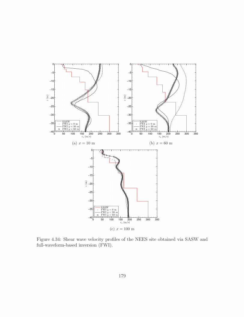
0 50 100 150 200 250 300 350−40
−35
−30
−25
−20
−15
−10
−5
0
z(m
)
cs (m/s)
SASWFWI y = 0 mFWI y = 30 mFWI y = 60 m
(a) x = 10 m
0 50 100 150 200 250 300 350−40
−35
−30
−25
−20
−15
−10
−5
0
z(m
)
cs (m/s)
SASWFWI y = 0 mFWI y = 30 mFWI y = 60 m
(b) x = 60 m
0 50 100 150 200 250 300 350−40
−35
−30
−25
−20
−15
−10
−5
0
z(m
)
cs (m/s)
SASWFWI y = 0 mFWI y = 30 mFWI y = 60 m
(c) x = 100 m
Figure 4.34: Shear wave velocity profiles of the NEES site obtained via SASW andfull-waveform-based inversion (FWI).
179
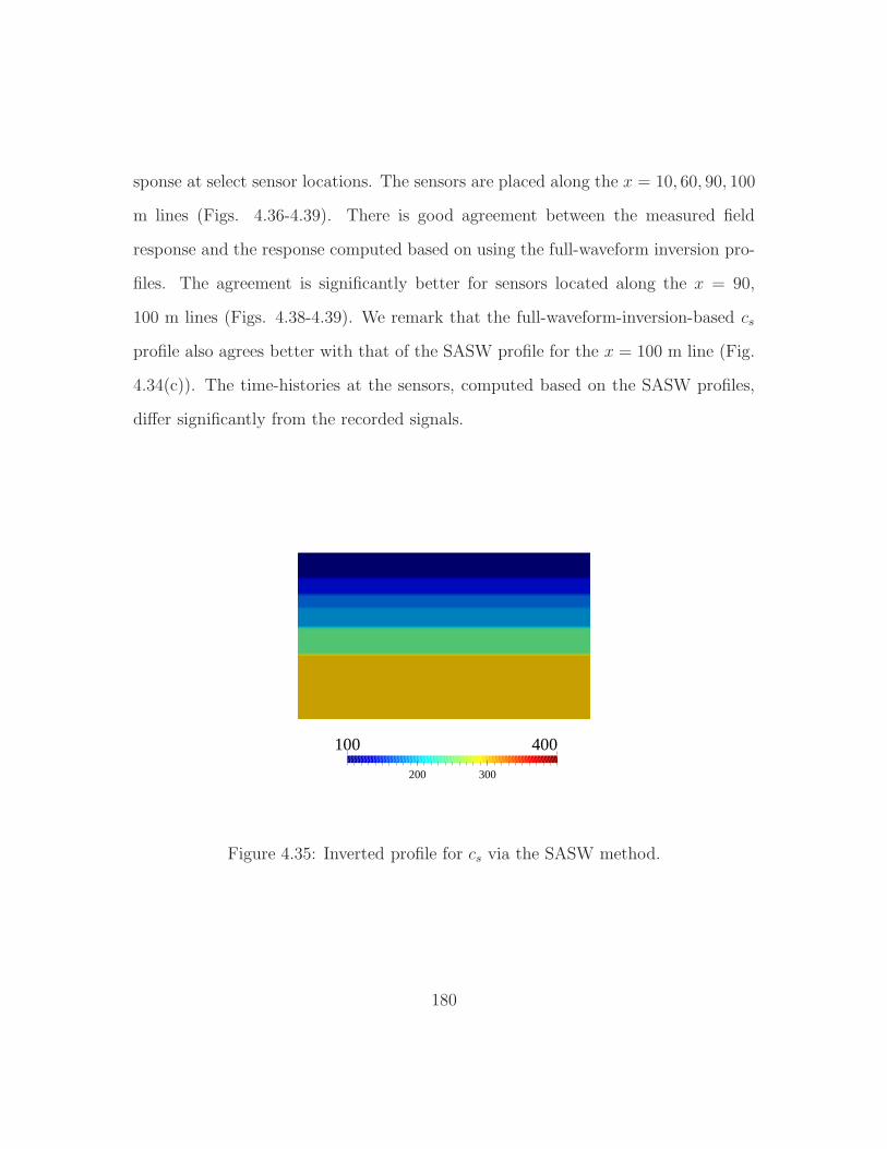
sponse at select sensor locations. The sensors are placed along the x = 10, 60, 90, 100
m lines (Figs. 4.36-4.39). There is good agreement between the measured field
response and the response computed based on using the full-waveform inversion pro-
files. The agreement is significantly better for sensors located along the x = 90,
100 m lines (Figs. 4.38-4.39). We remark that the full-waveform-inversion-based cs
profile also agrees better with that of the SASW profile for the x = 100 m line (Fig.
4.34(c)). The time-histories at the sensors, computed based on the SASW profiles,
differ significantly from the recorded signals.
200 300
100 400
Figure 4.35: Inverted profile for cs via the SASW method.
180
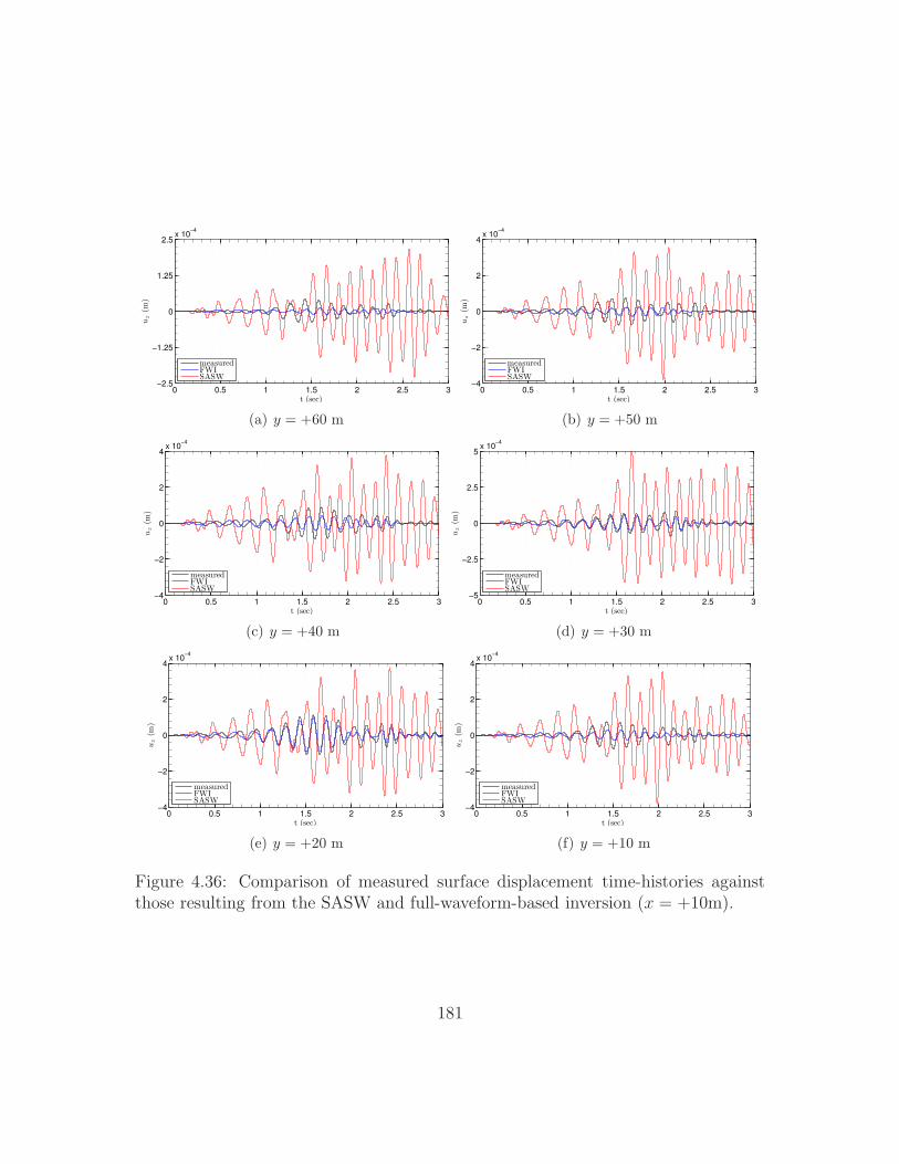
0 0.5 1 1.5 2 2.5 3−2.5
−1.25
0
1.25
2.5x 10
−4
t (sec)
uz
(m)
measuredFWISASW
(a) y = +60 m
0 0.5 1 1.5 2 2.5 3−4
−2
0
2
4x 10
−4
t (sec)
uz
(m)
measuredFWISASW
(b) y = +50 m
0 0.5 1 1.5 2 2.5 3−4
−2
0
2
4x 10
−4
t (sec)
uz
(m)
measuredFWISASW
(c) y = +40 m
0 0.5 1 1.5 2 2.5 3−5
−2.5
0
2.5
5x 10
−4
t (sec)
uz
(m)
measuredFWISASW
(d) y = +30 m
0 0.5 1 1.5 2 2.5 3−4
−2
0
2
4x 10
−4
t (sec)
uz
(m)
measuredFWISASW
(e) y = +20 m
0 0.5 1 1.5 2 2.5 3−4
−2
0
2
4x 10
−4
t (sec)
uz
(m)
measuredFWISASW
(f) y = +10 m
Figure 4.36: Comparison of measured surface displacement time-histories againstthose resulting from the SASW and full-waveform-based inversion (x = +10m).
181
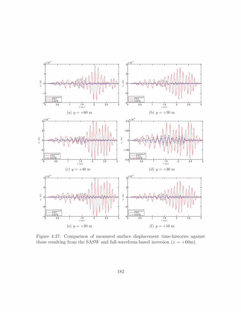
0 0.5 1 1.5 2 2.5 3−2
−1
0
1
2x 10
−4
t (sec)
uz
(m)
measuredFWISASW
(a) y = +60 m
0 0.5 1 1.5 2 2.5 3−4
−2
0
2
4x 10
−4
t (sec)
uz
(m)
measuredFWISASW
(b) y = +50 m
0 0.5 1 1.5 2 2.5 3−4
−2
0
2
4x 10
−4
t (sec)
uz
(m)
measuredFWISASW
(c) y = +40 m
0 0.5 1 1.5 2 2.5 3−2.5
−1.25
0
1.25
2.5x 10
−4
t (sec)
uz
(m)
measuredFWISASW
(d) y = +30 m
0 0.5 1 1.5 2 2.5 3−4
−2
0
2
4x 10
−4
t (sec)
uz
(m)
measuredFWISASW
(e) y = +20 m
0 0.5 1 1.5 2 2.5 3−4
−2
0
2
4x 10
−4
t (sec)
uz
(m)
measuredFWISASW
(f) y = +10 m
Figure 4.37: Comparison of measured surface displacement time-histories againstthose resulting from the SASW and full-waveform-based inversion (x = +60m).
182
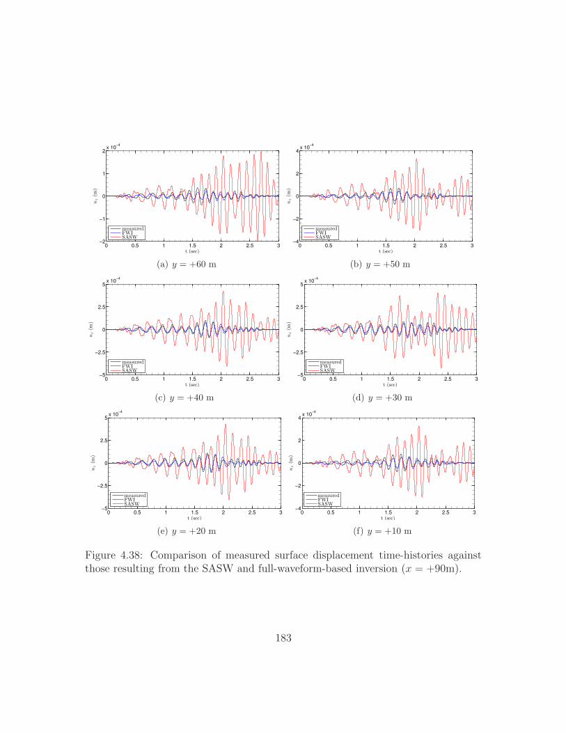
0 0.5 1 1.5 2 2.5 3−2
−1
0
1
2x 10
−4
t (sec)
uz
(m)
measuredFWISASW
(a) y = +60 m
0 0.5 1 1.5 2 2.5 3−4
−2
0
2
4x 10
−4
t (sec)
uz
(m)
measuredFWISASW
(b) y = +50 m
0 0.5 1 1.5 2 2.5 3−5
−2.5
0
2.5
5x 10
−4
t (sec)
uz
(m)
measuredFWISASW
(c) y = +40 m
0 0.5 1 1.5 2 2.5 3−5
−2.5
0
2.5
5x 10
−4
t (sec)
uz
(m)
measuredFWISASW
(d) y = +30 m
0 0.5 1 1.5 2 2.5 3−5
−2.5
0
2.5
5x 10
−4
t (sec)
uz
(m)
measuredFWISASW
(e) y = +20 m
0 0.5 1 1.5 2 2.5 3−4
−2
0
2
4x 10
−4
t (sec)
uz
(m)
measuredFWISASW
(f) y = +10 m
Figure 4.38: Comparison of measured surface displacement time-histories againstthose resulting from the SASW and full-waveform-based inversion (x = +90m).
183
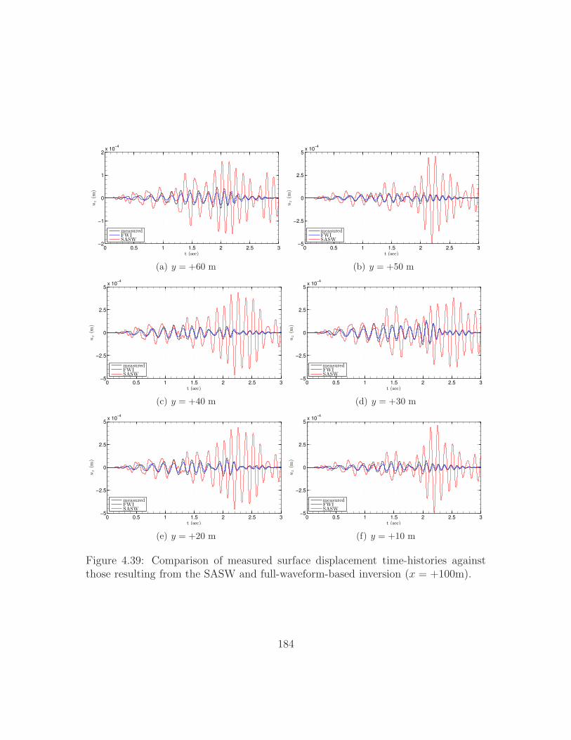
0 0.5 1 1.5 2 2.5 3−2
−1
0
1
2x 10
−4
t (sec)
uz
(m)
measuredFWISASW
(a) y = +60 m
0 0.5 1 1.5 2 2.5 3−5
−2.5
0
2.5
5x 10
−4
t (sec)
uz
(m)
measuredFWISASW
(b) y = +50 m
0 0.5 1 1.5 2 2.5 3−5
−2.5
0
2.5
5x 10
−4
t (sec)
uz
(m)
measuredFWISASW
(c) y = +40 m
0 0.5 1 1.5 2 2.5 3−5
−2.5
0
2.5
5x 10
−4
t (sec)
uz
(m)
measuredFWISASW
(d) y = +30 m
0 0.5 1 1.5 2 2.5 3−5
−2.5
0
2.5
5x 10
−4
t (sec)
uz
(m)
measuredFWISASW
(e) y = +20 m
0 0.5 1 1.5 2 2.5 3−5
−2.5
0
2.5
5x 10
−4
t (sec)
uz
(m)
measuredFWISASW
(f) y = +10 m
Figure 4.39: Comparison of measured surface displacement time-histories againstthose resulting from the SASW and full-waveform-based inversion (x = +100m).
184
4.6 Summary
We discussed recent advances in the development of a general and robust
methodology for geotechnical site characterization, based on full-waveform inversion,
using actual field data.
We considered two field experiments consistent with our code development:
firstly, we characterized the Hornsby Bend site in Austin, TX, by creating plane
strain field conditions and by assuming homogeneity lateral to a two-dimensional
slice. We discussed the design and post-processing needs of such field experiments,
so that collected records can be seamlessly integrated in the software toolchain.
Secondly, we reported the design of a field experiment aimed at the three-dimensional
characterization of the NEES@UCSB site in Garner Valley, CA, using the developed
three-dimensional inversion codes discussed in the preceding chapter.
Our results demonstrate the clear advantage of allowing for the imaging of
arbitrarily heterogeneous sites. Overall, our full-waveform-inversion-based site char-
acterization methodology seems robust and promising.
185
Chapter 5
Conclusions
5.1 Summary
We presented a robust methodology for site characterization using full-waveform
inversion. We complemented the theory and the numerical implementation with re-
sults derived from synthetic, as well as field data.
We developed PMLs for domain truncation of three-dimensional, arbitrarily
heterogeneous, elastic formations. The formulation is implemented in parallel, and
uses scalable algorithms, which makes it suitable for tackling large-scale problems.
Specifically, we use a displacement-stress formulation for the PML, coupled with a
standard displacement-only formulation for the PML. This hybrid treatment leads
to a cost-efficient computational scheme. We discuss several time-marching schemes,
which can be used a la carte, depending on the application: a) an extended Newmark
scheme for third-order in time, either unsymmetic or fully symmetric semi-discrete
forms; b) a standard implicit Newmark for second-order, unsymmetric semi-discrete
forms; and c) an explicit Runge-Kutta scheme for a first-order in time unsymmetric
system. We also discuss how our formulation can accommodate M-PML with simple
modifications. Using numerical experiments, we demonstrate stability and efficacy
of the proposed formulation.
186
Armed with a parallel state-of-the-art forward-wave-solver, we considered the
elastic inverse medium problem in three space dimensions. We cast the problem of
finding the distributed Lame parameters in an arbitrarily heterogeneous formation,
as a PDE-constraint optimization problem: elastic waves are used as probing agents
to interrogate the soil medium, and the response of the medium to these waves are
collected at receivers located on the ground surface. The inversion process relies
on minimizing a misfit between the collected response at receiver locations, and
a computed response based on a trial distribution of the Lame parameters. We
used strategies to alleviate ill-posedness, and lend algorithmic robustness to the
proposed inversion scheme. Specifically, we used (a) a regularization factor selection
and continuation scheme, where the regularization factor is adaptively computed
at each inversion iteration, based on a simple procedure; (b) a source-frequency
continuation scheme such that the inversion process evolves by using low-frequency
sources, and, gradually, we use sources with higher frequencies; and (c) a biasing
scheme for the λ search direction, such that, at early iterations of inversion, the
search direction for λ is biased based on that of µ. The latter strategy, in particular,
improves the reconstruction of the material profiles when simultaneous inversion of
the two Lame parameters is exercised. After verifying the accuracy of the computed
discrete gradients, by comparing them with directional finite differences, we reported
results demonstrating successful reconstruction of the Lame parameters for smooth
and sharp profiles, using both noise-free and highly-noisy data.
We also considered the inverse medium problem in two space dimensions,
followed by presenting a practical procedure to accommodate three-dimensional field
187
data into two-dimensional codes. We then presented inversion results pertaining
to a field experiment at the Hornsby Bend in Austin, TX, and compared them
against profiles obtained from the non-invasive SASW, and from invasive CPT tests.
Lastly, we used the methodology described in Chapter 3 for the three-dimensional
site characterization of the NEES@UCSB site in Garner Valley, CA. Overall, the
framework discussed in this study seems robust, practical, and promising.
5.2 Future directions
We suggest future directions that were outside the scope of this disserta-
tion, but are perceived as significant steps toward improving the proposed inversion
methodology.
• Validation: in an attempt to validate the proposed methodology, it is important
for the full-waveform-inversion-based profiles, obtained from the field experi-
ments, to be compared against invasive techniques that can also provide wave
velocity profiles, such as borehole methods.
• Uncertainty quantification: it is desirable to quantify how much confidence one
has in the inverted profiles. The Bayesian framework discussed in [106] seems
to be applicable to the methodology discussed in this work for quantifying
uncertainty in the inverted material profiles.
• Enhanced physics for wave simulation: reliable simulation of wave propagation
in soils is remarkably challenging. Even though soil is a lossy, porous medium
that is, oftentimes, partially saturated, it is usually idealized as an elastic solid.
188

Using models that can capture the complex physics of the soil more realistically,
is a significant improvement toward high-fidelity subsurface imaging.
• Multi-scale approach for inversion: in order to alleviate the ill-posedness in-
herent in inverse problems, and to minimize the risk of local minima trapping,
using a multi-scale approach, whereby the inversion process in carried out on
a sequence of finer grids, seems to be a viable approach [47].
189

Appendices
190
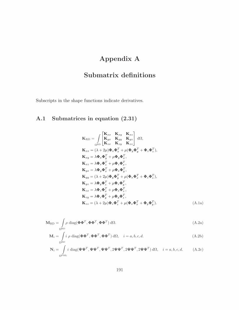
Appendix A
Submatrix definitions
Subscripts in the shape functions indicate derivatives.
A.1 Submatrices in equation (2.31)
KRD =
∫
ΩRD
Kxx Kxy Kxz
Kyx Kyy Kyz
Kzx Kzy Kzz
dΩ,
Kxx = (λ+ 2µ)ΦxΦTx + µ(ΦyΦ
Ty +ΦzΦ
Tz ),
Kxy = λΦxΦTy + µΦyΦ
Tx ,
Kxz = λΦxΦTz + µΦzΦ
Tx ,
Kyx = λΦyΦTx + µΦxΦ
Ty ,
Kyy = (λ+ 2µ)ΦyΦTy + µ(ΦxΦ
Tx +ΦzΦ
Tz ),
Kyz = λΦyΦTz + µΦzΦ
Ty ,
Kzx = λΦzΦTx + µΦxΦ
Tz ,
Kzy = λΦzΦTy + µΦyΦ
Tz ,
Kzz = (λ+ 2µ)ΦzΦTz + µ(ΦxΦ
Tx +ΦyΦ
Ty ). (A.1a)
MRD =
∫
ΩRD
ρ diag(ΦΦT ,ΦΦT ,ΦΦT ) dΩ. (A.2a)
Mi =
∫
ΩRD
i ρ diag(ΦΦT ,ΦΦT ,ΦΦT ) dΩ, i = a, b, c, d. (A.2b)
Ni =
∫
ΩPML
i diag(ΨΨT ,ΨΨT ,ΨΨT , 2ΨΨT , 2ΨΨT , 2ΨΨT ) dΩ, i = a, b, c, d. (A.2c)
191
Aiu =
∫
ΩPML
ΦxΨ
T λiyz ΦyΨ
T λixz ΦzΨ
T λixy
ΦyΨT λi
xz ΦxΨT λi
yz ΦzΨT λi
xy
ΦzΨT λi
xy ΦxΨT λi
yz ΦyΨT λi
xz
dΩ,
i = e, w, p, λejk = αjαk, λp
jk = αjβk + βjαk, λwjk = βjβk, j, k = x, y, z.
(A.3a)
Ail =
∫
ΩPML
Ax1 Ax2 Ax3 Ax4 Ax5
Ay1 Ay2 Ay3 Ay4 Ay6
Az1 Az2 Az3 Az5 Az6
dΩ, (A.4a)
Ax1 = (λ+ 2µ)ΦxΨT λi
yz, Ay1 = λΦyΨT λi
xz, Az1 = λΦzΨT λi
xy,
Ax2 = λΦxΨT λi
yz , Ay2 = (λ+ 2µ)ΦyΨT λi
xz, Az2 = λΦzΨT λi
xy,
Ax3 = λΦxΨT λi
yz , Ay3 = λΦyΨT λi
xz, Az3 = (λ+ 2µ)ΦzΨT λi
xy,
Ax4 = 2µΦyΨT λi
xz, Ay4 = 2µΦxΨT λi
yz , Az5 = 2µΦxΨT λi
yz ,
Ax5 = 2µΦzΨT λi
xy, Ay6 = 2µΦzΨT λi
xy, Az6 = 2µΦyΨT λi
xz ,
λejk = αjαk, λp
jk = αjβk + βjαk, λwjk = βjβk,
i = e, w, p, j, k = x, y, z. (A.5a)
fRD =
∫
ΓRD
N
Φ gx(x, t)Φ gy(x, t)Φ gz(x, t)
dΓ +
∫
ΩRD
Φ bx(x, t)Φ by(x, t)Φ bz(x, t)
dΩ. (A.6a)
A.2 Submatrices for the symmetric PML formulation
Ni =
∫
ΩPML
i
λ+µµ(3λ+2µ)ΨΨT −λ
2µ(3λ+2µ)ΨΨT −λ2µ(3λ+2µ)ΨΨT
−λ2µ(3λ+2µ)ΨΨT λ+µ
µ(3λ+2µ)ΨΨT −λ2µ(3λ+2µ)ΨΨT
−λ2µ(3λ+2µ)ΨΨT −λ
2µ(3λ+2µ)ΨΨT λ+µµ(3λ+2µ)ΨΨT
1µΨΨT
1µΨΨT
1µΨΨT
dΩ,
i = a, b, c, d.(A.7a)
192
Ai =
∫
ΩPML
ΦxΨ
T λiyz ΦyΨ
T λixz ΦzΨ
T λixy
ΦyΨT λi
xz ΦxΨT λi
yz ΦzΨT λi
xy
ΦzΨT λi
xy ΦxΨT λi
yz ΦyΨT λi
xz
dΩ,
i = e, w, p,
λejk = αjαk, λp
jk = αjβk + βjαk, λwjk = βjβk, j, k = x, y, z. (A.8a)
A.3 Submatrices for M-PML
Aiu =
∫
ΩPML
ΦxΨ
T λiyz ΦyΨ
T λixz ΦzΨ
T λixy
ΦyΨT λi
xz ΦxΨT λi
yz ΦzΨT λi
xy
ΦzΨT λi
xy ΦxΨT λi
yz ΦyΨT λi
xz
dΩ
+
∫
ΩPML
ΦΨT ∂λiyz
∂xΦΨT ∂λi
xz
∂yΦΨT ∂λi
xy
∂z
ΦΨT ∂λixz
∂yΦΨT ∂λi
yz
∂xΦΨT ∂λi
xy
∂z
ΦΨT ∂λixy
∂zΦΨT ∂λi
yz
∂xΦΨT ∂λi
xz
∂y
dΩ,
i = e, w, p, λejk = αjαk, λp
jk = αjβk + βjαk, λwjk = βjβk, j, k = x, y, z.
(A.9a)
A.4 Discretization of the control problems
In Section 3.2.1.3, we discussed the λ- and µ-control problems. In this part,we consider their spatial discretization. We use the basis function Φ for the spatialdiscretization of w(x, t) and u(x, t), and χ is the basis function for discretizing λ(x)and µ(x). For instance, if we approximate λ(x) with λh(x), then λh(x) = χTλ, whereλ comprises the vector of nodal values for λ. In the following, subscripts in the shapefunctions indicate derivatives, and uh = (uT
x ,uTy ,u
Tz )
T and wh = (wTx ,w
Ty ,w
Tz )
T isthe vector of discrete values of the state and adjoint variables, respectively. Accord-ingly
M =
∫
ΩRD
χχT dΩ. (A.10a)
193
For Tikhonov regularization:
gλreg =
∫
ΩRD
(χxχTx + χyχ
Ty + χzχ
Tz )λ dΩ, (A.10b)
gµreg =
∫
ΩRD
(χxχTx + χyχ
Ty + χzχ
Tz )µ dΩ. (A.10c)
For Total Variation regularization:
gλreg =
∫
ΩRD
(χxχTx + χyχ
Ty + χzχ
Tz )λ
(λT (χxχ
Tx + χyχ
Ty + χzχ
Tz )λ+ ǫ
) 1
2
dΩ, (A.10d)
gµreg =
∫
ΩRD
(χxχTx + χyχ
Ty + χzχ
Tz )µ
(µT (χxχ
Tx + χyχ
Ty + χzχ
Tz )µ+ ǫ
) 1
2
dΩ. (A.10e)
Moreover,
gλmis = −
∫ T
0
∫
ΩRD
χ (ΦTxwx +ΦT
ywy +ΦTz wz)(Φ
Txux +ΦT
y uy +ΦTz uz) dΩ dt,
(A.10f)
gµmis = −
∫ T
0
∫
ΩRD
χ(2 (ΦT
xwx ΦTxux +ΦT
ywy ΦTy uy +ΦT
z wz ΦTz uz)
+ (ΦTywx +ΦT
xwy)(ΦTxuy +ΦT
y ux) + (ΦTz wx +ΦT
xwz)(ΦTxuz +ΦT
z ux)
+ (ΦTz wy +ΦT
ywz)(ΦTy uz +ΦT
z uy))dΩ dt. (A.10g)
In (A.10a), upon using spectral elements with LGL quadrature rule, M becomesdiagonal; thus, its inverse can be computed easily.
A.5 Submatrices in equation (4.3)
The two-dimensional PML formulation discussed in Chapter 4, results in thesemi-discrete form (4.3), with the following definition for the system matrices:
194
M2D =
[MRD + Ma 0
0 −Na
], C2D =
[Mb Ae
ATe −Nb
], (A.11a)
K2D =
[KRD + Mc Ap
ATp −Nc
], (A.11b)
where a bar denotes matrix extension to encompass all the displacement degrees-of-freedom. The submatrices in (A.11) are defined below:
KRD =
∫
ΩRD
[(λ+ 2µ)ΦxΦ
Tx + µΦyΦ
Ty λΦxΦ
Ty + µΦyΦ
Tx
λΦyΦTx + µΦxΦ
Ty (λ+ 2µ)ΦyΦ
Ty + µΦxΦ
Tx
]dΩ, (A.12a)
MRD =
∫
ΩRD
ρ diag(ΦΦT ,ΦΦT ) dΩ, (A.12b)
Mi =
∫
ΩRD
i ρ diag(ΦΦT ,ΦΦT ) dΩ, i = a, b, c, (A.12c)
Ni =
∫
ΩPML
i
λ+2µ4µ(λ+µ)ΨΨT −λ
4µ(λ+µ)ΨΨT
−λ4µ(λ+µ)ΨΨT λ+2µ
4µ(λ+µ)ΨΨT
1µΨΨT
dΩ, i = a, b, c, (A.12d)
Ai =
∫
ΩPML
[ΦxΨ
T λiy ΦyΨ
T λix
ΦyΨT λi
x ΦxΨT λi
y
]dΩ, i = e, p, λe
j = αj , λpj = βj , j = x, y,
(A.12e)
where a = αxαy, b = αxβy + αyβx, and c = βxβy.
195
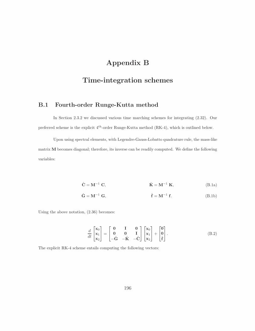
Appendix B
Time-integration schemes
B.1 Fourth-order Runge-Kutta method
In Section 2.3.2 we discussed various time marching schemes for integrating (2.32). Our
preferred scheme is the explicit 4th-order Runge-Kutta method (RK-4), which is outlined below.
Upon using spectral elements, with Legendre-Gauss-Lobatto quadrature rule, the mass-like
matrix M becomes diagonal; therefore, its inverse can be readily computed. We define the following
variables:
C = M−1 C, K = M−1 K, (B.1a)
G = M−1 G, f = M−1 f . (B.1b)
Using the above notation, (2.36) becomes:
d
dt
x0
x1
x2
=
0 I 00 0 I
−G −K −C
x0
x1
x2
+
00
f
. (B.2)
The explicit RK-4 scheme entails computing the following vectors:
196
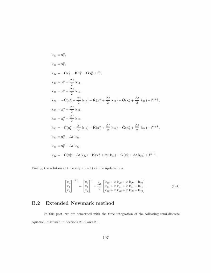
k10 = xn1 ,
k11 = xn2 ,
k12 = −Cxn2 − Kxn
1 − Gxn0 + fn,
k20 = xn1 +
∆t
2k11,
k21 = xn2 +
∆t
2k12,
k22 = −C(xn2 +
∆t
2k12)− K(xn
1 +∆t
2k11)− G(xn
0 +∆t
2k10) + fn+
1
2 ,
k30 = xn1 +
∆t
2k21,
k31 = xn2 +
∆t
2k22,
k32 = −C(xn2 +
∆t
2k22)− K(xn
1 +∆t
2k21)− G(xn
0 +∆t
2k20) + fn+
1
2 ,
k40 = xn1 +∆t k31,
k41 = xn2 +∆t k32,
k42 = −C(xn2 +∆t k32)− K(xn
1 +∆t k31)− G(xn0 +∆t k30) + fn+1.
Finally, the solution at time step (n+ 1) can be updated via
x0
x1
x2
n+1
=
x0
x1
x2
n
+∆t
6
k10 + 2 k20 + 2 k30 + k40
k11 + 2 k21 + 2 k31 + k41
k12 + 2 k22 + 2 k32 + k42
. (B.4)
B.2 Extended Newmark method
In this part, we are concerned with the time integration of the following semi-discrete
equation, discussed in Sections 2.3.2 and 2.5:
197
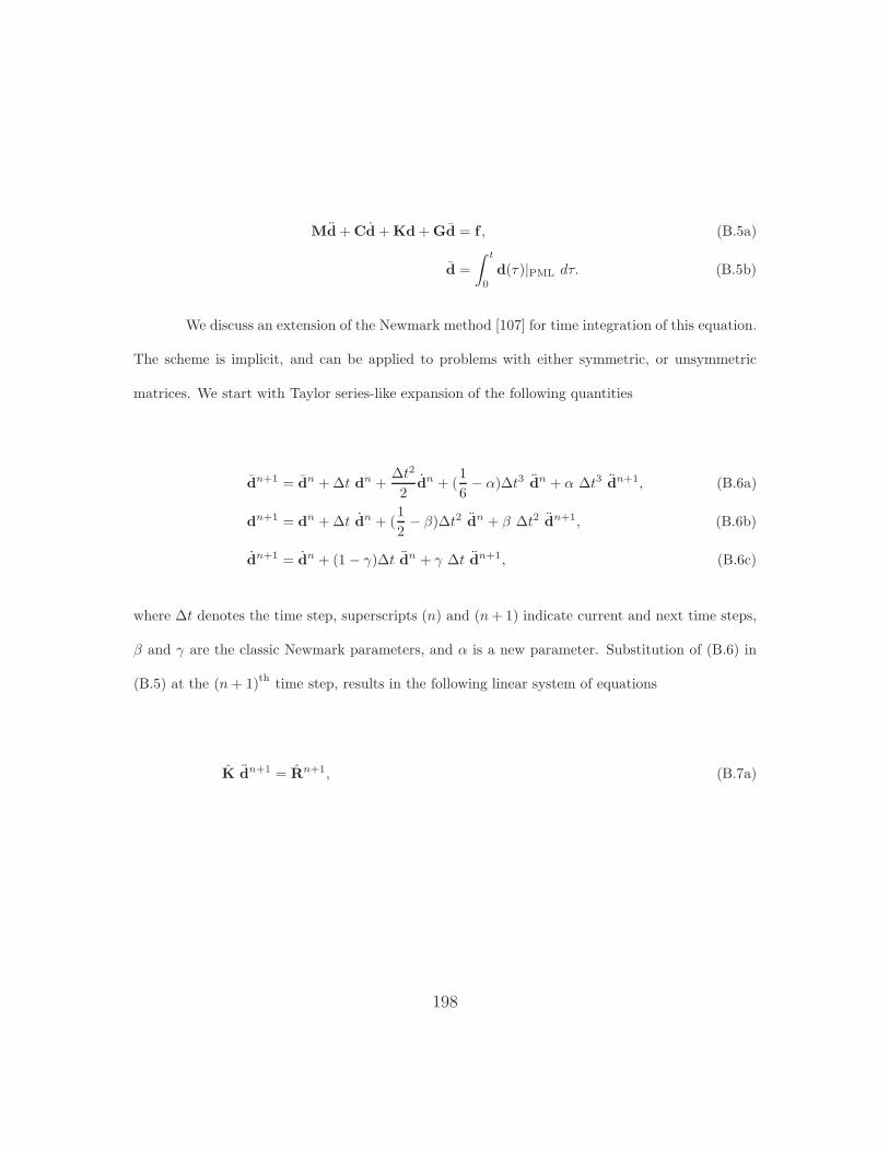
Md+Cd+Kd+Gd = f , (B.5a)
d =
∫ t
0
d(τ)|PML dτ. (B.5b)
We discuss an extension of the Newmark method [107] for time integration of this equation.
The scheme is implicit, and can be applied to problems with either symmetric, or unsymmetric
matrices. We start with Taylor series-like expansion of the following quantities
dn+1 = dn +∆t dn +∆t2
2dn + (
1
6− α)∆t3 dn + α ∆t3 dn+1, (B.6a)
dn+1 = dn +∆t dn + (1
2− β)∆t2 dn + β ∆t2 dn+1, (B.6b)
dn+1 = dn + (1 − γ)∆t dn + γ ∆t dn+1, (B.6c)
where ∆t denotes the time step, superscripts (n) and (n+ 1) indicate current and next time steps,
β and γ are the classic Newmark parameters, and α is a new parameter. Substitution of (B.6) in
(B.5) at the (n+ 1)th
time step, results in the following linear system of equations
K dn+1 = Rn+1, (B.7a)
198
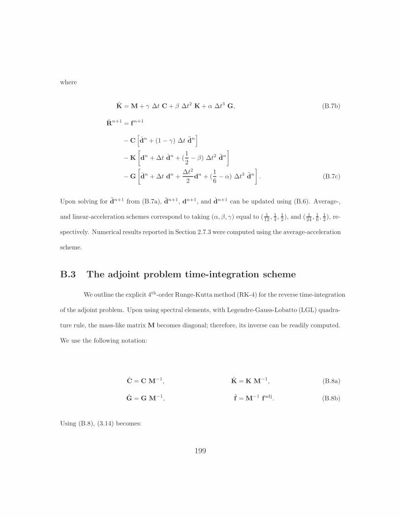
where
K = M+ γ ∆t C+ β ∆t2 K+ α ∆t3 G, (B.7b)
Rn+1 = fn+1
−C[dn + (1− γ) ∆t dn
]
−K
[dn +∆t dn + (
1
2− β) ∆t2 dn
]
−G
[dn +∆t dn +
∆t2
2dn + (
1
6− α) ∆t3 dn
]. (B.7c)
Upon solving for dn+1 from (B.7a), dn+1, dn+1, and dn+1 can be updated using (B.6). Average-,
and linear-acceleration schemes correspond to taking (α, β, γ) equal to ( 112 ,
14 ,
12 ), and ( 1
24 ,16 ,
12 ), re-
spectively. Numerical results reported in Section 2.7.3 were computed using the average-acceleration
scheme.
B.3 The adjoint problem time-integration scheme
We outline the explicit 4th-order Runge-Kutta method (RK-4) for the reverse time-integration
of the adjoint problem. Upon using spectral elements, with Legendre-Gauss-Lobatto (LGL) quadra-
ture rule, the mass-like matrix M becomes diagonal; therefore, its inverse can be readily computed.
We use the following notation:
C = C M−1, K = K M−1, (B.8a)
G = G M−1, f = M−1 fadj. (B.8b)
Using (B.8), (3.14) becomes:
199

d
dt
y0
y1
y2
=
0 I 00 0 I
GT −KT CT
y0
y1
y2
+
00
f
. (B.9)
The scheme entails computing the following vectors:
k10 = yn1 ,
k11 = yn2 ,
k12 = Cyn2 − Kyn
1 + Gyn0 + fn,
k20 = yn1 −
∆t
2k11,
k21 = yn2 −
∆t
2k12,
k22 = C(yn2 −
∆t
2k12)− K(yn
1 −∆t
2k11) + G(yn
0 −∆t
2k10) + fn−
1
2 ,
k30 = yn1 −
∆t
2k21,
k31 = yn2 −
∆t
2k22,
k32 = C(yn2 −
∆t
2k22)− K(yn
1 −∆t
2k21) + G(yn
0 −∆t
2k20) + fn−
1
2 ,
k40 = yn1 −∆t k31,
k41 = yn2 −∆t k32,
k42 = C(yn2 −∆t k32)− K(yn
1 −∆t k31) + G(yn0 −∆t k30) + fn−1.
Finally, the solution at time step (n− 1) can be updated via
y0
y1
y2
n−1
=
y0
y1
y2
n
− ∆t
6
k10 + 2 k20 + 2 k30 + k40
k11 + 2 k21 + 2 k31 + k41
k12 + 2 k22 + 2 k32 + k42
. (B.11)
200
Appendix C
Gradient of a functional
The gradient of a functional F : H → R, where H is a Hilbert space, is defined as the
Riesz-representation of the derivative F′(q)(q), such that
( G(q), q )H = F′(q)(q) ∀q ∈ H, (C.1)
where G denotes the gradient, and we use the following notation for the Gateaux derivative of F at
q in a direction q:
F′(q)(q) = lim
h→0
F(q+ hq)− F(q)
h. (C.2)
With this definition, it is not possible to talk about the gradient, without specifying the inner-
product utilized to represent the derivative [108].
201
Appendix D
On the third discrete optimality condition
We discuss the derivation of the discrete control equations, i.e., of the third discrete opti-
mality condition, given in (4.19) and (4.20). We take the derivative of L with respect to λ and µ
over the interior domain only, since the values of the Lame parameters at the interface nodes are
extended into the PML domain, without any variation along the direction of projection [57]. This
assumption greatly simplifies the derivation and implementation of the control equations.
The λ control problem
Equation (4.1a) governs the interior domain, denoted by ΩRD, where λ, µ only contribute
to terms in the K matrix of (4.3), which contributes to Q in (4.7). We denote the part of K that
belongs to the interior domain by KRD: it is the stiffness matrix of the interior problem, and is
given by [33]:
KRD =
∫
ΩRD
[(λTχ+ 2 µTχ) Φx1
ΦTx1
+ (µTχ) Φx3ΦT
x3. . .
(λTχ) Φx3ΦT
x1+ (µTχ) Φx1
ΦTx3
. . .
. . . (λTχ) Φx1ΦT
x3+ (µTχ) Φx3
ΦTx1
. . . (λTχ+ 2 µTχ) Φx3
ΦTx3
+ (µTχ) Φx1ΦT
x1
]dΩ, (D.1)
where χ is the vector of interpolation functions for the Lame parameters, Φ are the displacement
interpolants, and subscripts x1, x3 denote differentiation with respect to x1, and x3, respectively.
Taking the derivative of KRD with respect to λ, yields
202
∂KRD
∂λ=
∫
ΩRD
[Φx1
ΦTx1χ Φx1
ΦTx3χ
Φx3ΦT
x1χ Φx3
ΦTx3χ
]dΩRD, (D.2)
which are the building blocks of ∂
∂λ(pT Q d) in (4.19), thus enabling its computation.
The µ control problem
In a way similar to what we did above, we take the derivative of KRD with respect to µ to
obtain
∂KRD
∂µ=
∫
ΩRD
[2 Φx1
ΦTx1
+Φx3ΦT
x3
]χ Φx3
ΦTx1χ
Φx1ΦT
x3χ
[2 Φx3
ΦTx3
+Φx1ΦT
x1
]χ
dΩRD, (D.3)
thus allowing the computation of ∂∂µ(pT Q d) in (4.20).
203
Appendix E
On the singular convolution integral (4.21)
Due to the arrival of Raleigh waves, the integrand in (4.21) exhibits singularity. In this
part, we consider the integral in the Cauchy principal value sense, investigate the type of singularity,
and comment on the numerical evaluation of the integral. We repeat (4.21) with a small change in
notation:
u2D(x, t) =
∫ t
0
f2D(t− t′) G2D(x, t′) dt′, (E.1)
where G2D(x, t) is the Lamb Green’s function:
G2D(x, t) =cs
πµ|x|
0, τ < a−(2τ2−1)2
√τ2−a2
(2τ2−1)4+16τ4(τ2−a2)(1−τ2) , a ≤ τ ≤ 1−√τ2−a2
(2τ2−1)2−4τ2√τ2−a2
√τ2−1
, τ > 1,
where cs is shear wave velocity, µ is shear modulus, τ = tcs|x| is dimensionless time, a =
√1−2ν2−2ν
indicates the ratio of shear wave velocity to that of the compressional wave, and ν is Poisson’s
ratio.
In this section, we consider τ > 1, which contains the arrival time of the Rayleigh wave,
denoted by tR. Evaluation of (E.1) when τ ≤ 1 is straightforward. We split the integral into two
parts, the regular part and the singular part
204
u2D(x, t) =
∫
t\B(tR,ǫ)
f2D(t− t′) G2D(x, t′) dt′ +
∫
B(tR,ǫ)
f2D(t− t′) G2D(x, t′) dt′, (E.2)
where the singularity is isolated inside the ball B(tR, ǫ) = (tR − ǫ, tR + ǫ), where ǫ > 0 is “small”.
We focus on the singular integral. Since ǫ is “small”, we use the following approximation
∫
B(tR,ǫ)
f2D(t− t′) G2D(x, t′) dt′ ≈ f2D(t− tR)
∫
B(tR,ǫ)
G2D(x, t′) dt′. (E.3)
Next, we evaluate the following integral in the Cauchy principal value sense
Is = limǫ→0
∫
B(tR,ǫ)
G2D(x, t′) dt′, (E.4)
where
G2D(x, t′) =cs
πµ|x|−√τ2 − a2
(2τ2 − 1)2 − 4τ2√τ2 − a2
√τ2 − 1
. (E.5)
We rewrite the singular kernel (E.5) in the following form
G2D(x, t′) =Q
L−R=
Q(L+R)
(L−R)(L +R), (E.6)
where
Q =−csπµ|x|
√τ2 − a2, (E.7a)
L = (2τ2 − 1)2, (E.7b)
R = 4τ2√τ2 − a2
√τ2 − 1. (E.7c)
205

We investigate the case when L − R in (E.6) vanishes, i.e., (L − R)(L + R) = 0. We exploit the
following representation
(L−R)(L+R) = α(τ2 − ξ21)(τ2 − ξ22)(τ
2 − ξ23), (E.8)
where ξ2i , i = 1, 2, 3, are the roots of the corresponding polynomial on the left-hand-side, and α is
a scaling parameter. We associate ξ3 to the arrival time of the Rayleigh wave, and rewrite (E.6),
using (E.8), as follows
G2D(x, t′) =Q(L+R)
α(τ2 − ξ21)(τ2 − ξ22)(τ + ξ3)(τ − ξ3)
=φ(τ)
τ − ξ3, (E.9)
where
φ(τ) =Q(L+R)
α(τ2 − ξ21)(τ2 − ξ22)(τ + ξ3)
. (E.10)
We remark that the above representation is considered in B(tR, ǫ). Thus, φ(τ) is continuous, and
may be approximated with the following second order polynomial
φ(τ) = φ(t cs|x| ) ≈ a0 + a1t+ a2t
2, t ∈ B(tR, ǫ). (E.11)
Thus, (E.4) becomes
Is ≈|x|cs
limǫ→0
∫ tR+ǫ
tR−ǫ
a0 + a1t+ a2t2
t− tRdt. (E.12)
206
It can be shown that the above integral vanishes when evaluated in the Cauchy principal value
sense, i.e., the singularity is “weak”.
Next, we focus on the numerical evaluation of (E.1). In computer arithmetic, one cannot
approach infinitely close to the singular point. Thus, our strategy is to approximate the singular
integral analytically, inside a larger ball. To make the idea precise, let δ > ǫ, andB(tR, δ) ⊃ B(tR, ǫ),
where δ has the same order of magnitude that the time discretization has in the numerical evaluation
of the regular integral. Let t1 = inf B(tR, δ), and t2 = supB(tR, δ). Then, along the same lines, we
have
u2D(x, t) =
∫
t\B(tR,δ)
f2D(t− t′) G2D(x, t′) dt′ +
∫
B(tR,δ)
f2D(t− t′) G2D(x, t′) dt′. (E.13)
We define
Is =
∫
B(tR,δ)
f2D(t− t′) G2D(x, t′) dt′. (E.14)
Thus,
Is =
∫ tR−ǫ
t1
· · ·+∫
B(tR,ǫ)
· · ·+∫ t2
tR+ǫ
· · · , (E.15)
where · · · represents the integrand in (E.14). The second integral vanishes when evaluated in the
Cauchy principal value sense, as was shown earlier. It can be shown that the remaining terms can
be approximated as
207

Is ≈ f2D(t− tR)|x|cs
ln| t2 − tR
t1 − tR|(b0 + b1 tR + b2 t2R)
+ (t2 − t1)
(b1 + b2 (tR +
t2 + t12
)
), (E.16)
where b0, b1, and b2 are the coefficients of the polynomial that approximates φ(τ) in B(tR, δ). When
dealing with floating point arithmetic, the best approximation occurs when tR = 12 (t1 + t2), where
the logarithmic term vanishes.
208
Appendix F
On the spatial integration of (4.25)
We assume that the line load is applied along the x2 axis with a total length of 2L, and
that the observer is positioned along the x1 axis. We make the following change of variable to ease
the analytical integration:
G2L(x1, t) =
∫ L
−L
G3D(x1, x2, t) dx2 = 2
∫ rL
x1
G3D(r, t)r√
r2 − x21
dr, (F.1)
where, r =√x21 + x2
2, rL =√x21 + L2, and the Green’s function G3D is given as:
G3D(r, t) = B(r)
0 τ < a
u1 a ≤ τ ≤ 1
u∗2 1 ≤ τ ≤ ξ3
1 τ > ξ3
. (F.2)
We have the following definitions:
B(r) =1
rB∗ =
1
r
1− ν
2πµ, τ = t
csr,
u1 =1
2− 1
2
3∑
i=3
Ai√|τ2 − ξ2i |
, u∗2 = 1− A3√
ξ23 − τ2,
a =
√1− 2ν
2− 2ν, Ai =
(1− 2ξ2i )2√|a2 − ξ2i |
4(ξ2i − ξ2j )(ξ2i − ξ2k)
,
209
where ν is Poisson’s ration, µ is shear modulus, cs is shear wave velocity, and ξi are the roots of
the Rayleigh function:
R(ξ2) = (2ξ2 − 1)2 + 4√ξ2 − a2
√ξ2 − 1 = 0.
The above relations are valid when ν < 0.2631. In such a case, all roots are real and satisfy
0 < ξ21 < ξ22 < a2 < 1 < ξ23 [98]. Making use of Heaviside functions, we rewrite (F.2) as follows
G3D(r, t) = B(r)
−u1H
(r − tcs
a
)+ (u1 − u∗
2)H
(r − tcs
1
)+
(u∗2 − 1)H
(r − tcs
ξ3
)+ 1
. (F.3)
Substituting (F.3) into (F.1) yields
G2L(x1, t) = 2 (I1 + I2 + I3 + I4), (F.4)
where
I1 =1
2B∗
∫ rL
x1
−H(r − tcsa)√
r2 − x21
+
3∑
i=1
∫ rL
x1
Ai r H(r − tcsa)
ξi
√(t2c2sξ2i
− r2)(r2 − x21)
dr,
I2 =1
2B∗
∫ rL
x1
−H(r − tcs1 )√
r2 − x21
−2∑
i=1
∫ rL
x1
Ai r H(r − tcs1 )
ξi
√(t2c2sξ2i
− r2)(r2 − x21)
dr
+
∫ rL
x1
A3 r H(r − tcs1 )
ξ3
√(t2c2sξ23
− r2)(r2 − x21)
dr,
I3 = B∗∫ rL
x1
−A3 r H(r − tcsξ3
)
ξ3
√(t2c2sξ23
− r2)(r2 − x21)
dr,
210
I4 = B∗∫ rL
x1
dr√r2 − x2
1
.
It is easy to verify that I1, I2, I3, and I4 consist of the following integrals with the corresponding
closed-form solution
F1 =
∫r H(r − tcs
λ)√
(r2 − t2c2sξ2
)(r2 − x21)
dr =1
2H
(r − tcs
λ
)×
ln
(r2 − x21) + (r2 − t2c2s
ξ2) + 2
√(r2 − t2c2s
ξ2)(r2 − x2
1)
(t2c2sλ2 − x2
1) + (t2c2sλ2 − t2c2s
ξ2) + 2
√(t2c2sλ2 − t2c2s
ξ2)(
t2c2sλ2 − x2
1)
,
F2 =
∫r H(r − tcs
λ)√
−(r2 − t2c2sξ2
)(r2 − x21)
dr
= −1
2H
(r − tcs
λ
)tan−1
(t2c2sξ2− r2) + (x2
1 − r2)
2√(t2c2sξ2− r2)(r2 − x2
1)
+1
2H
(r − tcs
λ
)tan−1
(t2c2sξ2− t2c2s
λ2 ) + (x21 −
t2c2sλ2 )
2√(t2c2sξ2− t2c2s
λ2 )(t2c2sλ2 − x2
1)
,
F3 =
∫ √r2 − x2
1dr = ln(r +√r2 − x2
1),
F4 =
∫H
(r − tcs
λ
)√r2 − x2
1 dr = H
(r − tcs
λ
)
ln(r +√r2 − x2
1)
ln( tcsλ
+
√t2c2sλ2 − x2
1)
,
where λ takes the value of a, 1, or ξ3. Clearly, by exploiting the above closed-form expressions,
(4.25) can be evaluated accurately and efficiently.
211
Bibliography
[1] J. Bielak, R. W. Graves, K. B. Olsen, R. Taborda, L. Ramrez-Guzmn, S. M. Day, G. P. Ely,
D. Roten, T. H. Jordan, P. J. Maechling, J. Urbanic, Y. Cui, and G. Juve. The shakeout
earthquake scenario: Verification of three simulation sets. Geophysical Journal International,
180(1):375–404, 2010.
[2] U. Basu and A. K. Chopra. Perfectly matched layers for transient elastodynamics of un-
bounded domains. Int. J. Numer. Meth. Engng., 59:1039–1074, 2004.
[3] A. Fathi and V. Lotfi. Effects of reservoir length and rigorous fluid-foundation interaction on
the frequency response functions of concrete gravity dams. Dam Engineering, XXI(3):213–
233, January 2011.
[4] I. Epanomeritakis, V. Akcelik, O. Ghattas, and J. Bielak. A Newton-CG method for large-
scale three-dimensional elastic full-waveform seismic inversion. Inverse Problems, 24(3):034015,
2008.
[5] C. Jeong, L.F. Kallivokas, S. Kucukcoban, W. Deng, and A. Fathi. Maximization of wave
motion within a hydrocarbon reservoir for wave-based enhanced oil recovery. Journal of
Petroleum Science and Engineering, doi:10.1016/j.petrol.2015.03.009, 2015.
[6] P. M. Karve, S. Kucukcoban, and L. F. Kallivokas. On an inverse source problem for en-
hanced oil recovery by wave motion maximization in reservoirs. Computational Geosciences,
doi:10.1007/s10596-014-9462-7, 2014.
212
[7] P. M. Karve, , and L. F. Kallivokas. Wave energy focusing to subsurface poroelastic forma-
tions to promote oil mobilization. Geophysical Journal International, doi:10.1093/gji/ggv133,
2015.
[8] L.F. Kallivokas, A. Fathi, S. Kucukcoban, K.H. Stokoe II, J. Bielak, and O. Ghattas. Site
characterization using full waveform inversion. Soil Dynamics and Earthquake Engineering,
47:62 – 82, 2013.
[9] I. Harari, M. Slavutin, and E. Turkel. Analytical and numerical studies of a finite element
PML for the Helmholtz equation. Journal of Computational Acoustics, 8(1):121–137, 2000.
[10] D. Rabinovich, D. Givoli, and E. Becache. Comparison of high-order absorbing boundary
conditions and perfectly matched layers in the frequency domain. International Journal for
Numerical Methods in Biomedical Engineering, 26(10):1351–1369, 2010.
[11] F. Collino and P. B. Monk. Optimizing the perfectly matched layer. Computer Methods in
Applied Mechanics and Engineering, 164:157–171, 1998.
[12] P. G. Petropoulos. On the termination of the perfectly matched layer with local absorbing
boundary conditions. Journal of Computational Physics, 143(2):665–673, 1998.
[13] J.-P. Berenger. A perfectly matched layer for the absorption of electromagnetic waves.
Journal of Computational Physics, 114:185–200, 1994.
[14] W. C. Chew, J. M. Jin, and E. Michielssen. Complex coordinate system as a generalized
absorbing boundary condition. In Proc. 13th Annu. Rev. of Prog. Appl. Comp. Electromag.,
pages 909–914, Monterey,CA, 17-21 Mar. 1997. Vol. 2.
[15] W. C. Chew and W. H. Weedon. A 3D perfectly matched medium from modified Maxwell’s
equations with stretched coordinates. Micro. Opt. Tech. Lett., 7:599–604, 1994.
213
[16] F. L. Teixeira and W. C. Chew. Complex space approach to perfectly matched layers: a
review and some new developments. Int. J. Numer. Model., 13:441–455, 2000.
[17] W. C. Chew and Q. H. Liu. Perfectly matched layers for elastodynamics: a new absorbing
boundary condition. Journal of Computational Acoustics, 4(4):341–359, 1996.
[18] F. Collino and C. Tsogka. Application of the perfectly matched absorbing layer model to the
linear elastodynamic problem in anisotropic heterogeneous media. Geophysics, 66(1):294–
307, February 2001.
[19] F. Q. Hu. On absorbing boundary conditions for linearized Euler equations by a perfectly
matched layer. Journal of Computational Physics, 129:201–219, 1996.
[20] Y. Q. Zeng, J. Q. He, and Q. H. Liu. The application of the perfectly matched layer in
numerical modeling of wave propagation in poroelastic media. Geophysics, 66(4):1258–1266,
2001.
[21] S. D. Gedney. An anisotropic perfectly matched layer-absorbing medium for the truncation
of FDTD lattices. IEEE Transactions on Antennas and Propagation, 44(12):1630–1639,
December 1996.
[22] B. Gustafsson, H.-O. Kreiss, and J. Oliger. Time dependent problems and difference methods.
John Wiley & Sons, Inc., New York, 1995.
[23] S. Abarbanel and D. Gottlieb. A mathematical analysis of the PML method. Journal of
Computational Physics, 134(2):357 – 363, 1997.
[24] S. Abarbanel and D. Gottlieb. On the construction and analysis of absorbing layers in
CEM. Applied Numerical Mathematics, 27(4):331 – 340, 1998. Special Issue on Absorbing
Boundary Conditions.
214

[25] S. Abarbanel, D. Gottlieb, and J.S. Hesthaven. Long time behavior of the perfectly matched
layer equations in computational electromagnetics. Journal of Scientific Computing, 17(1-
4):405–422, 2002.
[26] K. Duru and G. Kreiss. A well-posed and discretely stable perfectly matched layer for elastic
wave equations in second order formulation. Communications in Computational Physics,
11(5):1643 – 1672, 2012.
[27] E. Becache, S. Fauqueux, and P. Joly. Stability of perfectly matched layers, group velocities
and anisotropic waves. Journal of Computational Physics, 188:399–433, 2003.
[28] F. H. Drossaert and A. Giannopoulos. A nonsplit complex frequency-shifted PML based
on recursive integration for FDTD modeling of elastic waves. Geophysics, 72(2):T9–T17,
March-April 2007.
[29] D. Komatitsch and R. Martin. An unsplit convolutional perfectly matched layer improved at
grazing incidence for the seismic wave equation. Geophysics, 72(5):SM155–SM167, September-
October 2007.
[30] T. Wang and X. Tang. Finite-difference modeling of elastic wave propagation: A nonsplitting
perfectly matched layer approach. Geophysics, 68(5):1749–1755, 2003.
[31] U. Basu. Explicit finite element perfectly matched layer for transient three-dimensional
elastic waves. Int. J. Numer. Meth. Engng., 77:151–176, 2009.
[32] R. Martin, D. Komatitsch, and S. D. Gedney. A variational formulation of a stabilized unsplit
convolutional perfectly matched layer for the isotropic or anisotropic seismic wave equation.
CMES, 37(3):274–304, 2008.
215
[33] S. Kucukcoban and L. F. Kallivokas. A symmetric hybrid formulation for transient wave
simulations in PML-truncated heterogeneous media. Wave Motion, 50:57–79, 2013.
[34] F. D. Hastings, J. B. Schneider, and S. L. Broschat. Application of the perfectly matched
layer (PML) absorbing boundary condition to elastic wave propagation. J. Acoust. Soc. Am.,
100(5):3061–3069, 1996.
[35] Q. H. Liu. Perfectly matched layers for elastic waves in cylindrical and spherical coordinates.
J. Acoust. Soc. Am., 105(4):2075–2084, April 1999.
[36] E. Becache, P. Joly, and C. Tsogka. Fictitious domains, mixed finite elements and per-
fectly matched layers for 2D elastic wave propagation. J. Comput. Acoust., 9(3):1175–1202,
September 2001.
[37] G. Festa and S. Nielsen. PML absorbing boundaries. Bulletin of the Seismological Society
of America, 93(2):891–903, April 2003.
[38] D. Komatitsch and J. Tromp. A perfectly matched layer absorbing boundary condition for
the second-order seismic wave equation. Geophysical Journal International, 154:146–153,
2003.
[39] G. Cohen and S. Fauqueux. Mixed spectral finite elements for the linear elasticity system in
unbounded domains. SIAM J. Sci. Comput., 26(3):864–884, 2005.
[40] G. Festa and J.-P. Vilotte. The Newmark scheme as velocity-stress time-staggering: an
efficient PML implementation for spectral element simulations of elastodynamics. Geophys.
J. Int., 161:789–812, 2005.
216
[41] K. C. Meza-Fajardo and A. S. Papageorgiou. A nonconvolutional, split-field, perfectly
matched layer for wave propagation in isotropic and anisotropic elastic media: Stability
analysis. Bulletin of the Seismological Society of America, 98(4):1811–1836, August 2008.
[42] D. Correia and J.-M. Jin. Performance of regular PML, CFS-PML, and second-order PML for
waveguide problems. Microwave and Optical Technology Letters, 48(10):2121–2126, October
2006.
[43] M.N. Dmitriev and V.V. Lisitsa. Application of M-PML reflectionless boundary conditions
to the numerical simulation of wave propagation in anisotropic media. part I: Reflectivity.
Numerical Analysis and Applications, 4(4):271–280, 2011.
[44] M.N. Dmitriev and V.V. Lisitsa. Application of M-PML absorbing boundary conditions
to the numerical simulation of wave propagation in anisotropic media. part II: Stability.
Numerical Analysis and Applications, 5(1):36–44, 2012.
[45] K. C. Meza-Fajardo and A. S. Papageorgiou. Study of the accuracy of the multiaxial perfectly
matched layer for the elastic-wave equation. Bulletin of the Seismological Society of America,
102(6):2458–2467, December 2012.
[46] P. Ping, Y. Zhang, and Y. Xu. A multiaxial perfectly matched layer (M-PML) for the
long-time simulation of elastic wave propagation in the second-order equations. Journal of
Applied Geophysics, 101:124 – 135, 2014.
[47] C. Bunks, F. Saleck, S. Zaleski, and G. Chavent. Multiscale seismic waveform inversion.
Geophysics, 60(5):1457–1473, 1995.
[48] R. E. Plessix. Introduction: Towards a full waveform inversion. Geophysical Prospecting,
56(6):761–763, 2008.
217
[49] A. Tarantola. Inversion of seismic reflection data in the acoustic approximation. Geophysics,
49(8):1259–1266, 1984.
[50] A. Fichtner, J. Trampert, P. Cupillard, E. Saygin, T. Taymaz, Y. Capdeville, and A. Villaseor.
Multiscale full waveform inversion. Geophysical Journal International, 2013.
[51] Q. Liu and Y. J. Gu. Seismic imaging: From classical to adjoint tomography. Tectonophysics,
566–567(0):31 – 66, 2012.
[52] P. Mora. Nonlinear two-dimensional elastic inversion of multioffset seismic data. Geophysics,
52(9):1211–1228, 1987.
[53] N. Rawlinson, S. Pozgay, and S. Fishwick. Seismic tomography: A window into deep earth.
Physics of the Earth and Planetary Interiors, 178(34):101 – 135, 2010.
[54] B. Banerjee, T. F. Walsh, W. Aquino, and M. Bonnet. Large scale parameter estimation
problems in frequency-domain elastodynamics using an error in constitutive equation func-
tional. Comp. Meth. Appl. Mech. Eng., 253:60–72, 2013.
[55] A. Gholami, A. Mang, and G Biros. Image-driven parameter estimation for low grade
gliomas. arXiv, 2014.
[56] J. W. Kang and L. F. Kallivokas. The inverse medium problem in heterogeneous PML-
truncated domains using scalar probing waves. Comput. Methods Appl. Mech. Engrg.,
200:265–283, 2011.
[57] S. Kucukcoban. The inverse medium problem in PML-truncated elastic media. Ph.D. thesis,
The University of Texas at Austin, 2010.
218
[58] S.-W. Na and L. F. Kallivokas. Direct time-domain soil profile reconstruction for one-
dimensional semi-infinite domains. Soil Dynamics and Earthquake Engineering, 29:1016–
1026, 2009.
[59] K. H. Stokoe II, S. G. Wright, J. A. Bay, and J. M. Roesset. Characterization of geotechnical
sites by SASW method. In R. D. Woods, editor, Geophysical Characterization of Sites, pages
15–25. Oxford & IBH Pub. Co., New Delhi, India, 1994.
[60] U. Albocher, P. E. Barbone, M. S. Richards, A. A. Oberai, and I. Harari. Approaches to
accommodate noisy data in the direct solution of inverse problems in incompressible plane
strain elasticity. Inverse Problems in Science and Engineering, 22(8):1307–1328, 2014.
[61] I. Epanomeritakis, V. Akcelik, O. Ghattas, and J. Bielak. A Newton-CG method for large-
scale three-dimensional elastic full-waveform seismic inversion. Inverse Problems, 24(3):034015,
2008.
[62] A. A. Oberai, N. H. Gokhale, M. M. Doyley, and M. Bamber. Evaluation of the adjoint
equation based algorithm for elasticity imaging. Physics in Medicine and Biology, 49:2955–
2974, 2004.
[63] A. A. Oberai, N. H. Gokhale, and G. R. Feijo. Solution of inverse problems in elasticity
imaging using the adjoint method. Inverse Problems, 19(2):297–313, 2003.
[64] K. T. Tran and M. McVay. Site characterization using Gauss-Newton inversion of 2-D full
seismic waveform in the time domain. Soil Dynamics and Earthquake Engineering, 43(0):16
– 24, 2012.
[65] R. G. Pratt, C. Shin, and G. J. Hick. GaussNewton and full Newton methods in frequencys-
pace seismic waveform inversion. Geophysical Journal International, 133(2):341–362, 1998.
219
[66] J. Bramwell. A Discontinuous Petrov-Galerkin Method for Seismic Tomography Problems.
Ph.D. thesis, The University of Texas at Austin, 2013.
[67] A. Fathi, B. Poursartip, and L. F. Kallivokas. Time-domain hybrid formulations for wave
simulations in three-dimensional PML-truncated heterogeneous media. International Journal
for Numerical Methods in Engineering, 101(3):165–198, 2015.
[68] N. Petra and G. Stadler. Model variational inverse problems governed by partial differential
equations. ICES Report 11-05, The Institute for Computational Engineering and Sciences,
The University of Texas at Austin, 2011.
[69] A. Fathi, L. F. Kallivokas, and B. Poursartip. Full-waveform inversion in three-dimensional
PML-truncated elastic media. Computer Methods in Applied Mechanics and Engineering,
(under review), 2015.
[70] A. Fathi, L. F. Kallivokas, K. H. Stokoe II, and B. Poursartip. Three-dimensional site
characterization using full-waveform inversion: theory, computations, and field experiments.
Soil Dynamics and Earthquake Engineering, (to be submitted), 2015.
[71] S. Kucukcoban and L.F. Kallivokas. Mixed perfectly-matched-layers for direct transient
analysis in 2D elastic heterogeneous media. Computer Methods in Applied Mechanics and
Engineering, 200(1-4):57–76, 2011.
[72] L. F. Kallivokas, J. Bielak, and R. C. MacCamy. A simple impedance-infinite element for
the finite element solution of the three-dimensional wave equation in unbounded domains.
Computer Methods in Applied Mechanics and Engineering, 147:235–262, 1997.
[73] F. Brezzi. A survey of mixed finite element methods. In D.L. Dwoyer, M.Y. Hussaini, and
R.G. Voigt, editors, Finite Elements Theory and Application, pages 34–49. Springer-Verlag,
220
New York, 1988.
[74] A. Quarteroni, R. Sacco, and F. Saleri. Numerical Mathematics. Texts in Applied Mathe-
matics. Springer, Berlin Heidelberg, second edition, 2007.
[75] A. Quarteroni and A. Valli. Numerical approximation of partial differential equations.
Springer Series in Computational Mathematics. Springer, Berlin Heidelberg, 2008.
[76] H. Bao, J. Bielak, O. Ghattas, L. F. Kallivokas, D. R. O’Hallaron, J. R. Shewchuk, and
J. Xu. Large-scale simulation of elastic wave propagation in heterogeneous media on parallel
computers. Comput. Methods Appl. Mech. Engrg., 152:85–102, 1998.
[77] D. A. Kopriva. Implementing spectral methods for partial differential equations. Springer,
2009.
[78] L.C. Wilcox, G. Stadler, C. Burstedde, and O. Ghattas. A high-order discontinuous Galerkin
method for wave propagation through coupled elastic-acoustic media. Journal of Computational
Physics, 229:9373–9396, 2010.
[79] R. Matzen. An efficient finite element time-domain formulation for the elastic second-order
wave equation: A non-split complex frequency shifted convolutional PML. International
Journal for Numerical Methods in Engineering, 88(10):951–973, 2011.
[80] M. Benzi, G. H. Golub, and J. Liesen. Numerical solution of saddle point problems. Acta
Numerica, pages 1–137, 2005.
[81] S. Balay, J. Brown, K. Buschelman, V. Eijkhout, W. D. Gropp, D. Kaushik, M. G. Knepley,
L. C. McInnes, B. F. Smith, and H. Zhang. PETSc users manual. Technical Report ANL-
95/11 - Revision 3.4, Argonne National Laboratory, 2013.
221

[82] E. Bozda, J. Trampert, and J. Tromp. Misfit functions for full waveform inversion based
on instantaneous phase and envelope measurements. Geophysical Journal International,
185(2):845–870, 2011.
[83] B. Engquist and B. Froese. Application of the Wasserstein metric to seismic signals.
Communications in Mathematical Science, 12(5):979–988, 2014.
[84] A. Tikhonov. Solution of incorrectly formulated problems and the regularization method.
Soviet Math. Dokl., 5:1035/1038, 1963.
[85] L. I. Rudin, S. Osher, and E. Fatemi. Nonlinear total variation based noise removal algo-
rithms. Phys. D, 60(1-4):259–268, November 1992.
[86] F. Troltzsch. Optimal Control of Partial Differential Equations: Theory, Methods, and
Applications, volume 112 of Graduate Studies in Mathematics. American Mathematical
Society, 2010.
[87] Z. Xie, D. Komatitsch, R. Martin, and R. Matzen. Improved forward wave propagation and
adjoint-based sensitivity kernel calculations using a numerically stable finite-element PML.
Geophysical Journal International, 198(3):1714–1747, 2014.
[88] V. Monteiller, S. Chevrot, D. Komatitsch, and N. Fuji. A hybrid method to compute short-
period synthetic seismograms of teleseismic body waves in a 3-D regional model. Geophysical
Journal International, 192(1):230–247, 2013.
[89] P. Tong, C. W. Chen, D. Komatitsch, P. Basini, and Q. Liu. High-resolution seismic
array imaging based on an SEM-FK hybrid method. Geophysical Journal International,
197(1):369–395, 2014.
222
[90] P. Tong, D. Komatitsch, T. L. Tseng, S. H. Hung, C. W. Chen, P. Basini, and Q. Liu. A
3-D spectral-element and frequency-wave number hybrid method for high-resolution seismic
array imaging. Geophysical Research Letters, 2014.
[91] Y. Choi, C. Farhat, W. Murray, and M. Saunders. A practical factorization of a Schur
complement for PDE-constrained distributed optimal control. arXiv, 2013.
[92] J. Nocedal and S. Wright. Numerical Optimization. Springer Series in Operations Research.
Springer, New York, NY, second edition, 2006.
[93] C. R. Vogel. Computational Methods for Inverse Problems. Frontiers in Applied Mathemat-
ics. Society for Industrial and Applied Mathematics (SIAM), Philadelphia, PA, 2002.
[94] M. D. Gunzburger. Perspectives in Flow Control and Optimization. Advances in Design and
Control. Society for Industrial and Applied Mathematics (SIAM), Philadelphia, PA, 2003.
[95] L. C. Wilcox, G. Stadler, T. Bui-Thanh, and O. Ghattas. Discretely exact derivatives for
hyperbolic PDE-constrained optimization problems discretized by the discontinuous Galerkin
method. arXiv, 2013.
[96] S. Kucukcoban and L. F. Kallivokas. Mixed perfectly-matched-layers for direct transient
analysis in 2D elastic heterogeneous media. Comput. Methods Appl. Mech. Engrg., 200:57–
76, 2011.
[97] G. Stadler. Personal communication, 2014.
[98] E. Kausel. Fundamental Solutions in Elastodynamics: a Compendium. Cambridge Univer-
sity Press, New York, NY, 2006.
[99] D. M. Boore and J. J. Bommer. Processing of strong-motion accelerograms: needs, options
and consequences. Soil Dynamics and Earthquake Engineering, 25:93–115, 2005.
223
[100] J. G. Proakis and D. K. Manolakis. Digital Signal Processing. Prentice Hall, Englewood
Cliffs, NJ, fourth edition, 2006.
[101] J. R. Krebs, J. E. Anderson, D. Hinkley, R. Neelamani, S. Lee, A. Baumstein, and M.-D. La-
casse. Fast full-wavefield seismic inversion using encoded sources. Geophysics, 74:WCC177–
WCC188, 2009.
[102] L. A. Romero, D. C. Ghiglia, C. C. Ober, and S. A. Morton. Phase encoding of shot records
in prestack migration. Geophysics, 65:426–436, 2000.
[103] G. Meles, S. Greenhalgh, J. van der Kruk, A. Green, and H. Mauerer. Taming the non-
linearity problem in GPR full-waveform inversion for high contrast media. Journal of Applied
Geophysics, 78:31–43, 2012.
[104] S. H. Joh. Advances in the data interpretation technique for spectral-analysis-of surface-waves
(SASW) measurements. Ph.D. thesis, The University of Texas at Austin, 1996.
[105] T. Lunne, P. K. Robertson, and J.J.M. Powell. Cone Penetration Testing in Geotechnical
Practice. Spon Press, London, 2002.
[106] T. Bui-Thanh, O. Ghattas, J. Martin, and G. Stadler. A computational framework for
infinite-dimensional Bayesian inverse problems part I: The linearized case, with application
to global seismic inversion. SIAM Journal on Scientific Computing, 35(6):A2494–A2523,
2013.
[107] D. Assimaki, L.F. Kallivokas, J.W. Kang, and S. Kucukcoban. Time-domain forward and
inverse modeling of lossy soils with frequency-independent Q for near-surface applications.
Soil Dynamics and Earthquake Engineering, 43:139–159, 2012.
224

[108] A. Borzi and V. Schulz. Computational Optimization of Systems Governed by Partial
Differential Equations. Computational Science and Engineering. Society for Industrial and
Applied Mathematics (SIAM), Philadelphia, PA, 2012.
225

Vita
Arash Fathi received his B.Sc. and M.Sc. degrees in Civil Engineering from Iran. He served
in Iran Army Corps of Engineers as a structural engineer for a year and a half, and has three years
of industrial experience with the dam and hydropower industry. In January 2009, he joined the
Department of Civil, Architectural and Environmental Engineering of the University of Texas at
Austin, to pursue a Ph.D. degree in Civil Engineering / Computational Mechanics, where he has
been working as a research and teaching assistant. He is a finalist of the 26th annual Robert J.
Melosh Medal competition for the best student paper on finite element analysis.
Permanent address: [email protected].
This dissertation was typeset with LATEX† by the author.
†LATEX is a document preparation system developed by Leslie Lamport as a special version ofDonald Knuth’s TEX Program.
226


