1

Lin Lin

Joint work with Roberto Car (Princeton), Joseph Morrone (Columbia) and Michele Parrinello (ETHZ)

Computational Research Division, Lawrence Berkeley National Lab

Displaced Path Integral Method for Computing the Momentum Distribution of Quantum Nuclei

Most molecular dynamics simulation treats nuclei as classical particles: Is this always a good approximation?

2

Classical statistical mechanics • NVT ensemble, partition function (single particle), 𝛽 = 1

𝑘𝐵𝑇

𝑍 = ∫ 𝑑𝑑 𝑑𝑑 𝑒−𝛽 𝑝2

2𝑚+𝑉 𝑥

• Free energy

𝐹 = −1𝛽

log𝑍 = −1𝛽

log2𝑚𝑚𝛽

12−

1𝛽

log ∫ 𝑑𝑑 𝑒−𝛽𝑉(𝑥)

• Classical statistical mechanics predicts NO isotope effect

3

Experimental evidence of nuclear quantum effects

Courtesy of Joseph Morrone

4

Classical statistical mechanics • Momentum distribution (Maxwell-Boltzmann form)

𝑛 𝒑′ = 𝛿 𝒑 − 𝒑′ = 1𝑍∫ 𝑑𝒑 𝑑𝒙𝛿 𝒑 − 𝒑′ 𝑒

−𝛽 𝒑𝟐

2𝑚+𝑉 𝒙

=𝛽

2𝑚𝑚

32𝑒−

𝛽𝒑22𝑚

• Radial momentum distribution

𝑛 𝑑 =𝑑2

4𝑚∫ 𝑑Ω 𝑛 𝒑 =

𝛽2𝑚𝑚

32𝑑2𝑒−

𝛽𝑝22𝑚

5

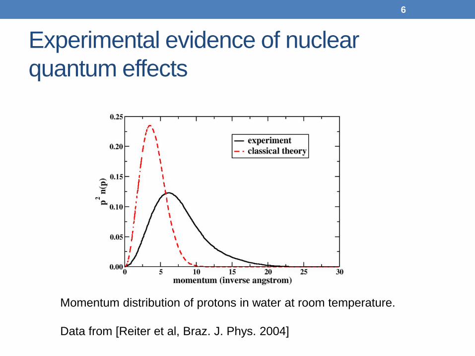
Experimental evidence of nuclear quantum effects

Momentum distribution of protons in water at room temperature. Data from [Reiter et al, Braz. J. Phys. 2004]

6

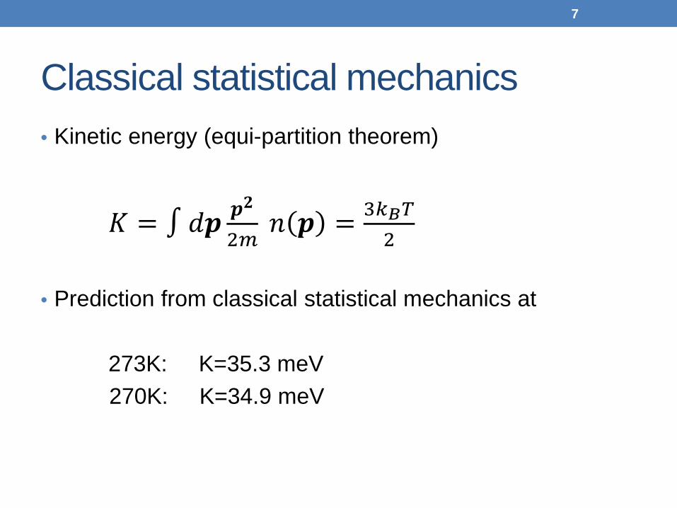
Classical statistical mechanics • Kinetic energy (equi-partition theorem)

𝐾 = ∫ 𝑑𝒑 𝒑𝟐

2𝑚 𝑛 𝒑 = 3𝑘𝐵𝑇

2

• Prediction from classical statistical mechanics at

273K: K=35.3 meV 270K: K=34.9 meV

7

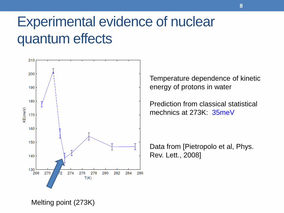
Experimental evidence of nuclear quantum effects

Temperature dependence of kinetic energy of protons in water Prediction from classical statistical mechnics at 273K: 35meV Data from [Pietropolo et al, Phys. Rev. Lett., 2008]

Melting point (273K)

8

Hydrogen atoms (and other light atoms) should be treated as quantum particles. How to compute the momentum distribution of quantum nuclei?

9

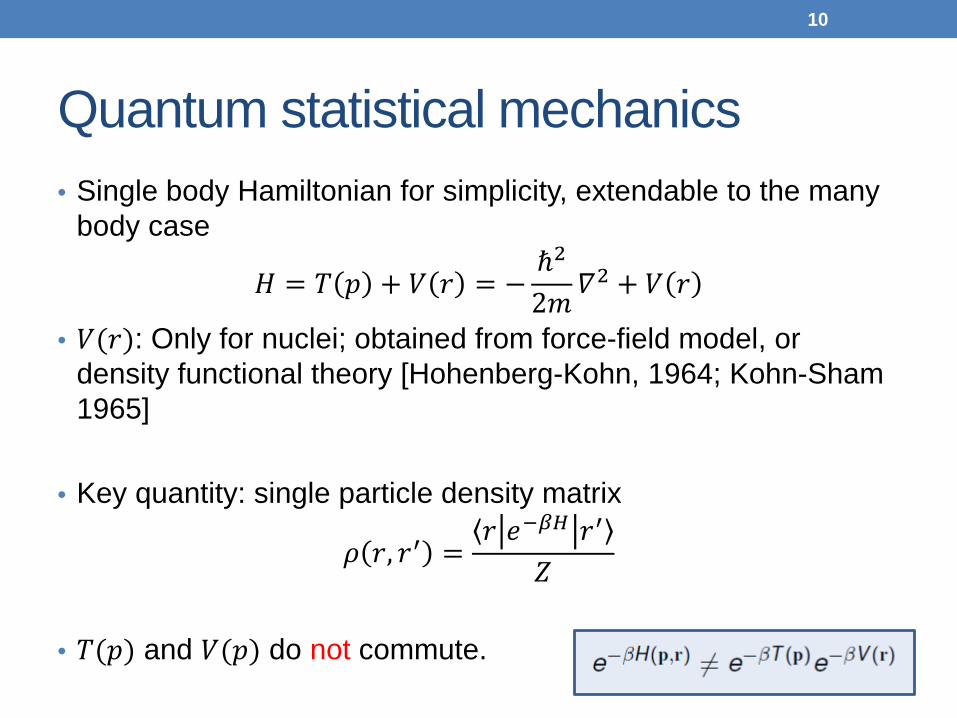
Quantum statistical mechanics • Single body Hamiltonian for simplicity, extendable to the many

body case

𝐻 = 𝑇 𝑑 + 𝑉 𝑟 = −ℏ2

2𝑚𝛻2 + 𝑉 𝑟

• 𝑉(𝑟): Only for nuclei; obtained from force-field model, or density functional theory [Hohenberg-Kohn, 1964; Kohn-Sham 1965]

• Key quantity: single particle density matrix

𝜌 𝑟, 𝑟′ =𝑟 𝑒−𝛽𝛽 𝑟′

𝑍

• 𝑇(𝑑) and 𝑉(𝑑) do not commute.

10

Trotter expansion (Strang splitting)

𝑒−𝛽𝛽 = lim𝑃→∞

Π𝑖𝑃𝑒−𝛽𝑃𝛽 = lim

𝑃→∞Π𝑖𝑃𝑒

− 𝛽2𝑃𝑉 𝑟 𝑒−

𝛽𝑃𝑇 𝑝 𝑒−

𝛽2𝑃𝑉 𝑟

Insert P-1 unity operators 𝐼 = ∫ 𝑑𝑟𝑖|𝑟𝑖⟩⟨𝑟𝑖| 𝜌 𝑟, 𝑟′

=1𝑍

lim𝑃→∞

∫ 𝑑𝑟2 ⋯𝑑𝑟𝑃�𝑒−𝛽2𝑃𝑉 𝑟𝑖

𝑃

𝑖=1

⟨𝑟𝑖|𝑒−𝛽𝑃𝑇 𝑝 𝑟𝑖+1 𝑒−

𝛽2𝑃𝑉 𝑟𝑖+1

𝑟1 = 𝑟, 𝑟𝑃+1 = 𝑟′

11

Trotter expansion (Strang splitting)

𝑟𝑖| 𝑒−𝛽𝑃𝑇(𝑝) |𝑟𝑖+1 ∝ 𝑒

− 𝑚𝑃2𝛽ℏ2 𝑟𝑖−𝑟𝑖+1

2

𝜌 𝑟, 𝑟′ ∝ lim𝑃→∞

∫ 𝑑𝑟2 ⋯𝑑𝑟𝑃𝑒−𝛽𝑈𝑒𝑒𝑒

𝑈𝑒𝑒𝑒 = �𝑚𝑚2𝛽ℏ2

𝑟𝑖 − 𝑟𝑖+1 2 +12𝑚

𝑉 𝑟1 + 𝑉 𝑟𝑃+1

𝑃

𝑖=1

Quantum-Classical isomorphism [Chandler and Wolynes, J Chem Phys,1981] Continuous form: Feynman path along imaginary time

12

Molecular dynamics Introduce a set of (fictitious) masses {𝑚𝑖}

lim𝑃→∞

∫ 𝑑𝑟1𝑑𝑟2 ⋯𝑑𝑟𝑃𝑑𝑟𝑃+1𝑒−𝛽𝑈𝑒𝑒𝑒

∝ lim𝑃→∞

∫ 𝑑𝑑1𝑑𝑑2 ⋯𝑑𝑑𝑃𝑑𝑑𝑃+1𝑑𝑟1𝑑𝑟2 ⋯𝑑𝑟𝑃𝑑𝑟𝑃+1𝑒−𝛽(∑

𝑝𝑖2

2𝑚𝑖+𝑖 𝑈𝑒𝑒𝑒)

Newton’s equation (quantum-to-classical isomorphism)

𝑟�̇� =𝑑𝑖𝑚𝑖

𝑑�̇� = −𝜕𝑈𝑒𝑒𝑒𝜕𝑟𝑖

+ 𝑡𝑡𝑒𝑟𝑚𝑡𝑡𝑡𝑡𝑡

13

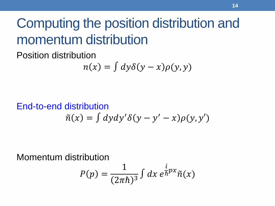
Computing the position distribution and momentum distribution Position distribution

𝑛 𝑑 = ∫ 𝑑𝑑𝛿 𝑑 − 𝑑 𝜌(𝑑,𝑑) End-to-end distribution

𝑛� 𝑑 = ∫ 𝑑𝑑𝑑𝑑′𝛿 𝑑 − 𝑑′ − 𝑑 𝜌(𝑑,𝑑′) Momentum distribution

𝑚 𝑑 =1

2𝑚ℏ 3 ∫ 𝑑𝑑 𝑒𝑖ℏ𝑝𝑥𝑛�(𝑑)

14

Open and closed path

“Open” path Sample 𝜌 𝑟, 𝑟′ Momentum distribution

“Closed” path Sample 𝜌(𝑟, 𝑟) Position distribution

15

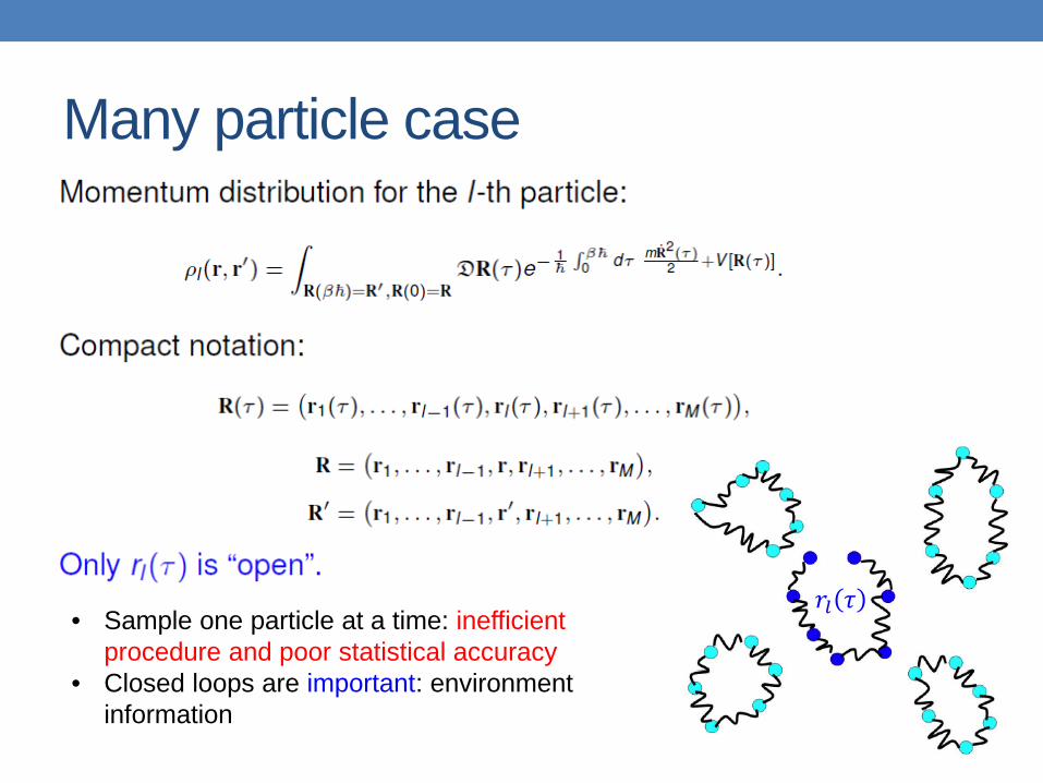
Many particle case

𝑟𝑙 𝜏 • Sample one particle at a time: inefficient

procedure and poor statistical accuracy • Closed loops are important: environment

information

Alternative methods? • Can we compute the end-to-end distribution only with

closed path integrals? ⇒ Perturbation theory.

• Naïve perturbation method does not work: infinite variance in the continuous limit

Displaced path formulation • End-to-end distribution

• Key idea: Add uniform displacement to the whole path 𝑑 𝜏 = 1

2− 𝜏

𝛽ℏ.

[LL-Morrone-Car-Parrinello, Phys. Rev. Lett. 2010]

Interpretation of the displaced path formulation • 𝑛 𝑑 = 𝑒−

𝑚𝑥2

2𝛽ℏ2 𝑍 𝑥𝑍(0)

; 𝑈 𝑑 = −log 𝑍 𝑥𝑍(0)

is precisely the free energy difference corresponding to the order parameter x.

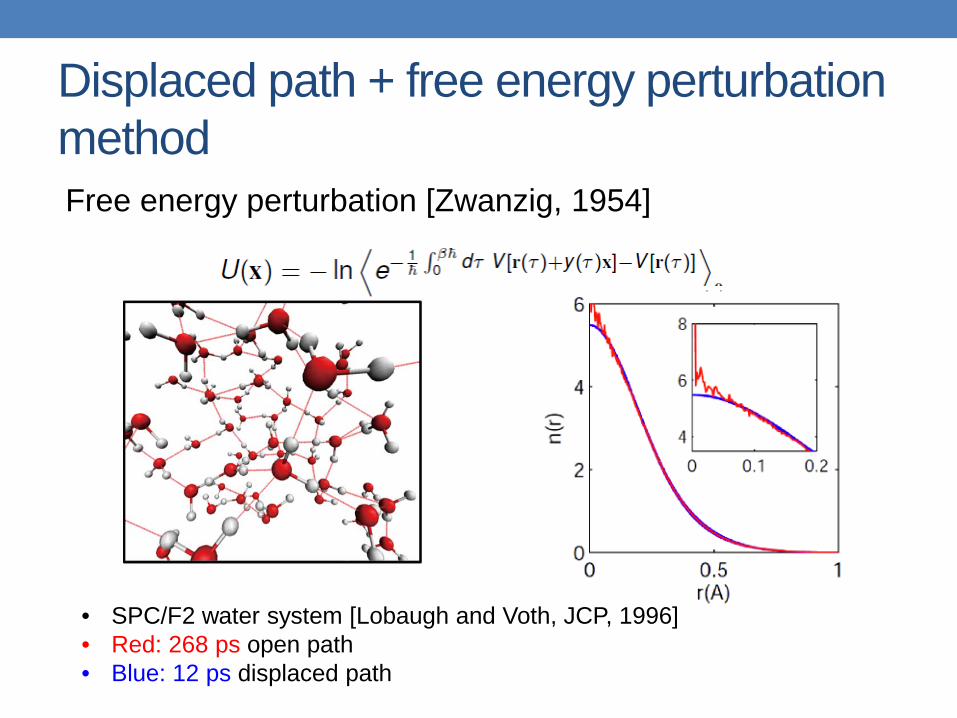
Displaced path + free energy perturbation method

• SPC/F2 water system [Lobaugh and Voth, JCP, 1996] • Red: 268 ps open path • Blue: 12 ps displaced path

Free energy perturbation [Zwanzig, 1954]

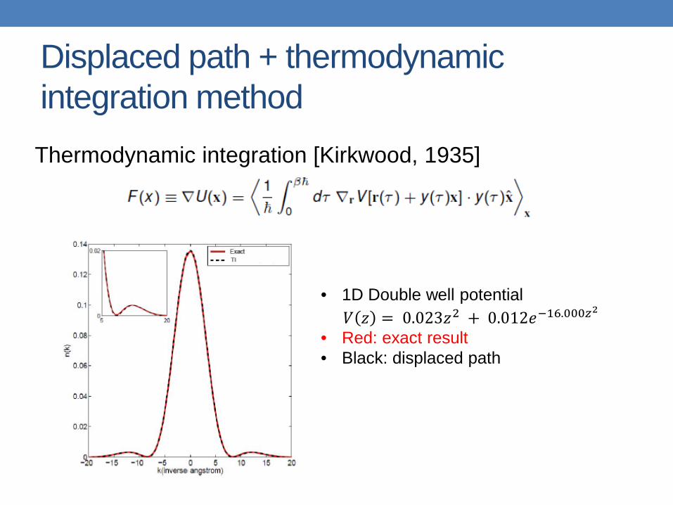
Displaced path + thermodynamic integration method

• 1D Double well potential 𝑉 𝑧 = 0.023𝑧2 + 0.012𝑒−16.000𝑧2

• Red: exact result • Black: displaced path

Thermodynamic integration [Kirkwood, 1935]

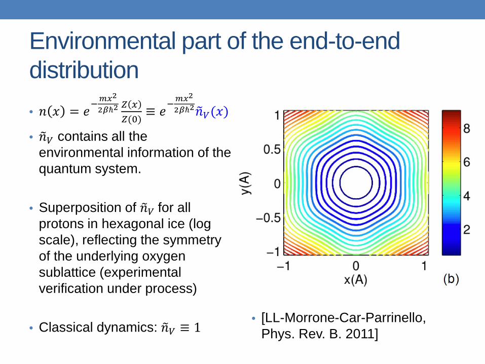
Environmental part of the end-to-end distribution • 𝑛 𝑑 = 𝑒−

𝑚𝑥2

2𝛽ℏ2 𝑍 𝑥𝑍(0)

≡ 𝑒−𝑚𝑥2

2𝛽ℏ2𝑛�𝑉(𝑑)

• 𝑛�𝑉 contains all the environmental information of the quantum system.

• Superposition of 𝑛�𝑉 for all protons in hexagonal ice (log scale), reflecting the symmetry of the underlying oxygen sublattice (experimental verification under process)

• Classical dynamics: 𝑛�𝑉 ≡ 1

• [LL-Morrone-Car-Parrinello, Phys. Rev. B. 2011]

Conclusion • Displaced path integral method: efficient and accurate

method for estimating the momentum distribution

• Directional character: useful for crystal system.

• Factorized free particle and environmental contribution

• Improve the applicability of the free energy perturbation method using enhanced sampling technique for displaced path method [LL-Quah-Car-Parrinello, in preparation]

Acknowledgment Luis Alvarez fellowship supported by LBNL and DOE.

Thank you for your attention!