Embed Size (px)
Citation preview
University of Cape Town
Masters Thesis
Dispersion measure variations in pulsarobservations with LOFAR
Author:
Abubakr Ibrahim
Supervisors:
Dr Maciej Serylak
Dr Shazrene Mohamed
A thesis submitted in fulfilment of the requirements
for the degree of MSc (Astrophysics)
in the
Faculty of Science
Department of Astronomy
April 2019
Univers
ity of
Cap
e Tow
n

The copyright of this thesis vests in the author. No quotation from it or information derived from it is to be published without full acknowledgement of the source. The thesis is to be used for private study or non-commercial research purposes only.
Published by the University of Cape Town (UCT) in terms of the non-exclusive license granted to UCT by the author.
Univers
ity of
Cap
e Tow
n

Declaration of Authorship
I, Abubakr Ibrahim, declare that this thesis titled, ’Dispersion measure variations in
pulsar observations with LOFAR’ and the work presented in it is my own.“I confirm that
this work submitted for assessment is my own and is expressed in my own words. Any
uses made within it of the works of other authors in any form (e.g., ideas, equations,
figures, text, tables, programs) are properly acknowledged at any point of their use. A
list of the references employed is included”.
Signed:
Date:
i

“Not only are we in the universe, the universe is in us. I don’t know of any deeper
spiritual feeling than what that brings upon me.”
Neil deGrasse Tyson, Astrophysicist
UNIVERSITY OF CAPE TOWN
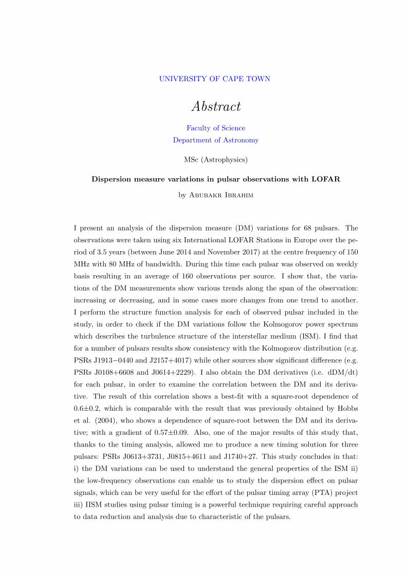
Abstract
Faculty of Science
Department of Astronomy
MSc (Astrophysics)
Dispersion measure variations in pulsar observations with LOFAR
by Abubakr Ibrahim
I present an analysis of the dispersion measure (DM) variations for 68 pulsars. The
observations were taken using six International LOFAR Stations in Europe over the pe-
riod of 3.5 years (between June 2014 and November 2017) at the centre frequency of 150
MHz with 80 MHz of bandwidth. During this time each pulsar was observed on weekly
basis resulting in an average of 160 observations per source. I show that, the varia-
tions of the DM measurements show various trends along the span of the observation:
increasing or decreasing, and in some cases more changes from one trend to another.
I perform the structure function analysis for each of observed pulsar included in the
study, in order to check if the DM variations follow the Kolmogorov power spectrum
which describes the turbulence structure of the interstellar medium (ISM). I find that
for a number of pulsars results show consistency with the Kolmogorov distribution (e.g.
PSRs J1913−0440 and J2157+4017) while other sources show significant difference (e.g.
PSRs J0108+6608 and J0614+2229). I also obtain the DM derivatives (i.e. dDM/dt)
for each pulsar, in order to examine the correlation between the DM and its deriva-
tive. The result of this correlation shows a best-fit with a square-root dependence of
0.6±0.2, which is comparable with the result that was previously obtained by Hobbs
et al. (2004), who shows a dependence of square-root between the DM and its deriva-
tive; with a gradient of 0.57±0.09. Also, one of the major results of this study that,
thanks to the timing analysis, allowed me to produce a new timing solution for three
pulsars: PSRs J0613+3731, J0815+4611 and J1740+27. This study concludes in that:
i) the DM variations can be used to understand the general properties of the ISM ii)
the low-frequency observations can enable us to study the dispersion effect on pulsar
signals, which can be very useful for the effort of the pulsar timing array (PTA) project
iii) IISM studies using pulsar timing is a powerful technique requiring careful approach
to data reduction and analysis due to characteristic of the pulsars.
Acknowledgements
First of all, I would like to express my deepest appreciation to my supervisor Dr Maciej
Serylak, for giving me an opportunity of working in this wonderful project, and for his
patient, guidance and generosity for being always available for me during the entire
period of the project. I would also like to extend my deepest appreciation to my co-
supervisor Dr Shazrene Mohamed, for her numerous efforts on taking care of all the
official and scientific inputs, and making sure the project is flowing smoothly even during
the leave. I’m also grateful to all the members of EPTA IISM group for their useful
inputs, comments, and help throughout the project. Especially, I’m extremely grateful
to Dr Caterina Tiburzi for her incredible willingness in helping me every time I need it.
Special thanks to Dr Marisa Geyer for being a very kind and generous person in helping
me in all the aspects during the period of my project. I also want to thanks Dr Lucas
Guillemot, Prof. Joris Verbiest, Dr James McKee, Dr Jean-Mathias Griessmeier, Sarah
Buchner and Prof. Aris Karastergiou, for their help and valuable comments. I want
to thanks my colleague Isabella Rammala for the fabulous environment and for being
so helpful when we chat about pulsars. Thanks, Issac for the accompany and all my
NASSPies colleagues. I gratefully acknowledge: the National Astrophysics and Space
Science Program (NASSP) for the generous funding of my project, and the International
LOFAR Stations: FR606, SE607, DE601, DE602, DE603, and DE605, for providing me
with the data. I’d like to recognize the supports of the Square Kilometer Array South
Africa (SKA SA) office and the South African Astronomical Observatory (SAAO) for
hosting my project and providing me with the necessary equipment to complete my
research study. Finally, grateful thanks to my lovely family and friends for always being
supportive all the time.
iv
Contents
Declaration of Authorship i
Abstract iii
Acknowledgements iv
Contents v
List of Figures vii
List of Tables viii
1 Introduction 1
2 Pulsars and Neutron Stars 4
2.1 Discovery . . . . . . . . . . . . . . . . . . . . . . . . . . . . . . . . . . . . 4
2.2 Pulsar and Neutron Star Properties . . . . . . . . . . . . . . . . . . . . . 5
2.2.1 Basic Properties . . . . . . . . . . . . . . . . . . . . . . . . . . . . 6
2.2.2 Rotating Dipole Model . . . . . . . . . . . . . . . . . . . . . . . . . 8
2.2.3 The Galactic Distribution . . . . . . . . . . . . . . . . . . . . . . . 9
2.3 Pulsar Categories . . . . . . . . . . . . . . . . . . . . . . . . . . . . . . . . 10
2.3.1 P -P Diagram . . . . . . . . . . . . . . . . . . . . . . . . . . . . . 11
2.3.2 Normal Pulsars . . . . . . . . . . . . . . . . . . . . . . . . . . . . . 11
2.3.3 Millisecond Pulsars (MSPs) . . . . . . . . . . . . . . . . . . . . . . 11
2.3.4 Magnetars . . . . . . . . . . . . . . . . . . . . . . . . . . . . . . . . 13
2.3.5 Rotating Radio Transients (RRATs) . . . . . . . . . . . . . . . . . 15
2.4 Interstellar Medium (ISM) . . . . . . . . . . . . . . . . . . . . . . . . . . . 15
2.4.1 Dispersion . . . . . . . . . . . . . . . . . . . . . . . . . . . . . . . . 16
2.4.2 Scattering . . . . . . . . . . . . . . . . . . . . . . . . . . . . . . . . 17
2.4.3 Scintillation . . . . . . . . . . . . . . . . . . . . . . . . . . . . . . . 19
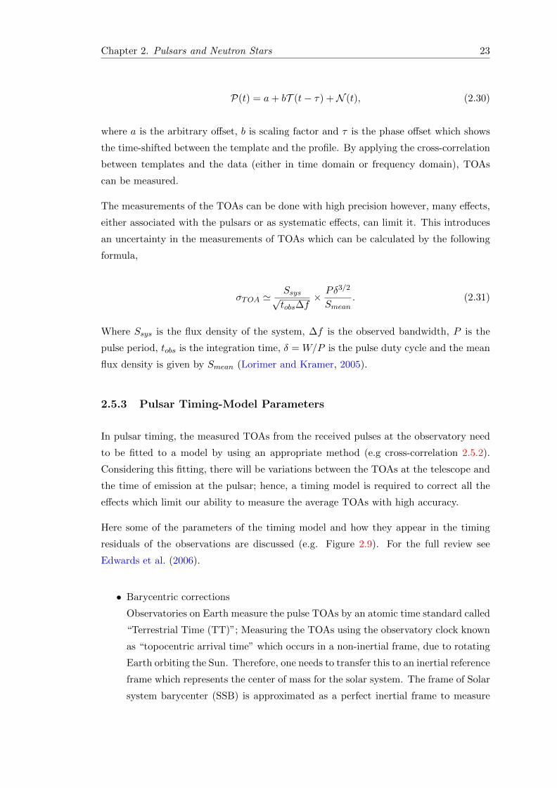
2.5 Pulsar Timing . . . . . . . . . . . . . . . . . . . . . . . . . . . . . . . . . . 21
2.5.1 Time of Arrivals (TOAs) . . . . . . . . . . . . . . . . . . . . . . . 22
2.5.2 Template Matching . . . . . . . . . . . . . . . . . . . . . . . . . . . 22
2.5.3 Pulsar Timing-Model Parameters . . . . . . . . . . . . . . . . . . . 23
v
Contents vi
3 Observations and Data Reduction 26
3.1 LOw Frequency ARray (LOFAR) . . . . . . . . . . . . . . . . . . . . . . . 26
3.2 Observations . . . . . . . . . . . . . . . . . . . . . . . . . . . . . . . . . . 31
3.2.1 Observations with French Station (FR606) . . . . . . . . . . . . . 31
3.2.2 Observations with Swedish Station (SE607) . . . . . . . . . . . . . 32
3.2.3 Observations with the LOFAR Stations in Germany . . . . . . . . 33
3.3 Data Reduction . . . . . . . . . . . . . . . . . . . . . . . . . . . . . . . . . 34
3.3.1 Data Processing . . . . . . . . . . . . . . . . . . . . . . . . . . . . 34
4 Data Analysis and Results 40
4.1 Data Analysis . . . . . . . . . . . . . . . . . . . . . . . . . . . . . . . . . . 40
4.1.1 Timing and DM Measurements . . . . . . . . . . . . . . . . . . . . 40
4.2 Results . . . . . . . . . . . . . . . . . . . . . . . . . . . . . . . . . . . . . . 43
4.2.1 New Timing Solutions for LOTAS/LOTAAS Sources . . . . . . . . 43
4.2.2 Nulling in PSR J1900+2600 . . . . . . . . . . . . . . . . . . . . . . 44
4.2.3 DM and DM Derivatives (dDM/dt) . . . . . . . . . . . . . . . . . 44
4.2.4 Structure Function . . . . . . . . . . . . . . . . . . . . . . . . . . . 50
4.2.5 DM Variations and the Solar Angle . . . . . . . . . . . . . . . . . . 51
5 Discussion and Conclusions 54

List of Figures
1.1 The ISM Dispersion Effect . . . . . . . . . . . . . . . . . . . . . . . . . . . 2
2.1 First Detection of Pulsar . . . . . . . . . . . . . . . . . . . . . . . . . . . . 5
2.2 Goldreich-Julian Model . . . . . . . . . . . . . . . . . . . . . . . . . . . . 8
2.3 Magnetosphere Model of Pulsars . . . . . . . . . . . . . . . . . . . . . . . 9
2.4 Galactic Distribution of Pulsars . . . . . . . . . . . . . . . . . . . . . . . . 10
2.5 P -P Diagram . . . . . . . . . . . . . . . . . . . . . . . . . . . . . . . . . . 12
2.6 Formation Model of the Binary Systems . . . . . . . . . . . . . . . . . . . 14
2.7 ISM Dispersion . . . . . . . . . . . . . . . . . . . . . . . . . . . . . . . . . 18
2.8 Scattering Model . . . . . . . . . . . . . . . . . . . . . . . . . . . . . . . . 19
2.9 Timing Model Parameters . . . . . . . . . . . . . . . . . . . . . . . . . . . 25
3.1 Distribution of LOFAR Stations . . . . . . . . . . . . . . . . . . . . . . . 28
3.2 The Core and International Stations of LOFAR . . . . . . . . . . . . . . . 29
3.3 Data Reduction Diagram . . . . . . . . . . . . . . . . . . . . . . . . . . . 36
3.4 Diagnostic Report . . . . . . . . . . . . . . . . . . . . . . . . . . . . . . . 38
3.5 RFI Effects . . . . . . . . . . . . . . . . . . . . . . . . . . . . . . . . . . . 39
4.1 The Standard Profile of J0139+5814 . . . . . . . . . . . . . . . . . . . . . 42
4.2 DM Variations . . . . . . . . . . . . . . . . . . . . . . . . . . . . . . . . . 45
4.3 DM Variations . . . . . . . . . . . . . . . . . . . . . . . . . . . . . . . . . 46
4.4 DM Derivative . . . . . . . . . . . . . . . . . . . . . . . . . . . . . . . . . 47
4.5 The Correlation between DM and DM Derivative . . . . . . . . . . . . . 50
4.6 The Structure Functions . . . . . . . . . . . . . . . . . . . . . . . . . . . . 52
4.7 Gaussian Process (GP) Regression . . . . . . . . . . . . . . . . . . . . . . 53
4.8 DM and Solar Position . . . . . . . . . . . . . . . . . . . . . . . . . . . . 53
vii
List of Tables
3.1 Data from FR606 . . . . . . . . . . . . . . . . . . . . . . . . . . . . . . . . 32
3.2 Data from SE607 . . . . . . . . . . . . . . . . . . . . . . . . . . . . . . . . 33
3.3 Data from German LOFAR Stations . . . . . . . . . . . . . . . . . . . . . 35
4.1 New Timing Solutions . . . . . . . . . . . . . . . . . . . . . . . . . . . . . 44
4.2 DM Derivative I . . . . . . . . . . . . . . . . . . . . . . . . . . . . . . . . 48
4.3 DM Derivative II . . . . . . . . . . . . . . . . . . . . . . . . . . . . . . . . 49
viii

This thesis is dedicated to . . .
The sake of Allah, my Creator and my Master;
My Parents: Yagob & Shama;My lovely Sisters, Brothers and my Friends.
ix
Chapter 1
Introduction
The interstellar medium (ISM) is the matter, radiation and magnetic fields that occupy
the space between the stellar systemss in a galaxy. When the radio emission from a
pulsar reaches an observer on Earth, it has propagated through different components
of the ISM. Throughout this propagation, the emission from pulsar interacts with the
free electrons in the ionized gas of the ISM. As a result, three main effects of the ISM
on the emission from pulsars can be observed. These effects are scattering, scintillation
and dispersion (e.g. Lorimer and Kramer 2005).
The last mentioned case i.e. dispersion, can be seen clearly in the frequency-resolved
pulse profile from radio pulsars. This effect is best noticeable in delay between emitted
pulses at lower frequencies, which arrive later, and the pulses emitted at the higher
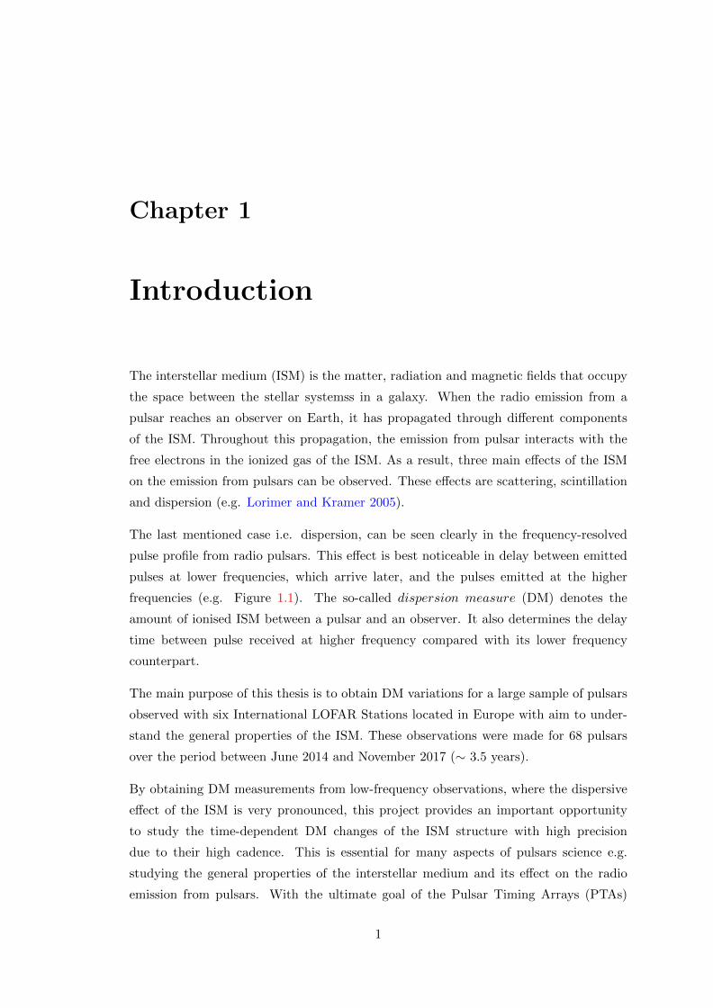
frequencies (e.g. Figure 1.1). The so-called dispersion measure (DM) denotes the
amount of ionised ISM between a pulsar and an observer. It also determines the delay
time between pulse received at higher frequency compared with its lower frequency
counterpart.
The main purpose of this thesis is to obtain DM variations for a large sample of pulsars
observed with six International LOFAR Stations located in Europe with aim to under-
stand the general properties of the ISM. These observations were made for 68 pulsars
over the period between June 2014 and November 2017 (∼ 3.5 years).
By obtaining DM measurements from low-frequency observations, where the dispersive
effect of the ISM is very pronounced, this project provides an important opportunity
to study the time-dependent DM changes of the ISM structure with high precision
due to their high cadence. This is essential for many aspects of pulsars science e.g.
studying the general properties of the interstellar medium and its effect on the radio
emission from pulsars. With the ultimate goal of the Pulsar Timing Arrays (PTAs)
1
Chapter 1. Introduction 2
Figure 1.1: The effect of the ISM dispersion on the received signal from PSRJ1921+2153. The plot shows the dispersion in the frequency profile, where the re-ceived pulse at lower frequencies arrive later than the emitted pulses at the higherfrequencies. The gaps along the pulses of this plot are removed frequency channels due
to RFI. This pulsar is included in this study.
projects aiming to detect the stochastic gravitational waves (GWs) background using
so-called high-precision pulsar timing, precisely characterizing DM using low-frequency
observations, similar to those used in this study, can greatly improve pulsar timing at
higher frequencies. Such study was shown in Cordes et al. (2016), where the analysis of
the frequency dependence of the DM showed rms DM difference of ∼ 4× 10⁻⁵ pc cm−3
across number of frequency bands near 1.5 GHz for pulsars at ∼ 1 kpc distance. The
obtained arrival-time variations were ranged as: i) from few to hundreds of nanosecond
for DM ≤ 30 pc cm−3 (with rapidly increasing to microseconds) ii) more than hundreds
nanosecond for larger DM as well as wider frequency bands.
This thesis is divided into five chapters as follows:
Chapter 2 contains five sections, wherein the first section I present an overview about
pulsars and their first discovery and their distribution. In the second and third sections, I
show the basic properties of pulsars and their main categories, respectively. In the fourth
section, I introduce the interstellar medium and its effects on the pulsar observations.
While in section five I present the concept of pulsar timing.
Chapter 3 is split into three sections. The first section introduces the Low-Frequency
Array (LOFAR) telescope with a brief description of its components and its functionality.
A full description of the data used in this thesis and their reduction is introduced in the

Chapter 1. Introduction 3
second and third section respectively.
Chapter 4 contains two sections. In the first section, I give a detailed description of the
data analysis. The results and the outcomes of this study are presented in the second
section.
Chapter 5 contains of the conclusion and the discussion of the study.
Chapter 2
Pulsars and Neutron Stars
Pulsars are highly magnetized and rapidly rotating neutron stars which emit across a
wide range of wavelengths. Most pulsars are observed in the radio part of the electro-
magnetic spectrum, but some also known to emit at optical wavelengths, X-rays and
gamma-rays. Their radiation can be observed when a beam of emission crosses the path
toward observer. In this Chapter, the discovery of pulsars is presented in § 2.1. The
basic properties of pulsars are given in § 2.2, and their population in § 2.3. The inter-
stellar medium and their effects on pulse propagation are presented in § 2.4, and a brief
overview of pulsar timing is also given in § 2.5.
2.1 Discovery
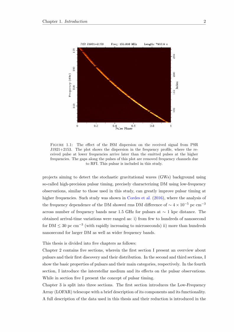
The discovery of the pulsars was made by Jocelyn Bell in July 1967 (Hewish et al., 1968),
while she was investigating the scintillation of radio signals from quasars caused by the
irregular structure of the interplanetary medium (e.g. Figure 2.1). This investigation
was carried out with the Mullard Radio Astronomy Observatory which operated at a
frequency of 81 MHz. Four months later in November, after systematic investigation
and analysis a very stable pulse signal with a period of 1.337 seconds was revealed. The
nature of this signal was first considered to be an extra-terrestrial intelligence signal
or terrestrial signal reflected off the Moon, but none of these theories was accepted.
Instead, the authors stated that:“A tentative explanation of these unusual sources in
terms of the stable oscillations of white dwarf or neutron stars is proposed”.
In 1934, two astronomers, Walter Baade and Fritz Zwicky, suggested a new type of star
as a result of the supernova explosion of a massive star (Baade and Zwicky, 1934). Since
then, many studies (e.g Oppenheimer and Volkoff, 1939) have supported this model. In
their study, Oppenheimer and Volkoff used the equation of state (EoS) for a cold Fermi
4
Chapter 2. Pulsars and Neutron Stars 5
gas, to show that a quasi-static solution is required to interpret the collapse of a large
mass into a small and dense core. This ultimately enabled them to predict the density
and the total mass of the resulting star. In 1967, Pacini (1967) also suggested that a
high dense stellar core with a strong magnetic field could be the product of a supernova
explosion and as the result, it could be the source of the energy in the Crab Nebula.
These studies indicate that a spinning neutron star could be the origin of the discovered
pulsar.
Figure 2.1: The observation of the first discovered pulsar. (a) The first recordingof PSR 1919+21; initially the signal resembled the radio interference also seen on thischart. (b) Fast chart recording showing individual pulses as downward deflections of
the trace (Hewish et al., 1968).
2.2 Pulsar and Neutron Star Properties
In this section, a general overview of pulsar properties will be introduced in § 2.2.1.
Also, a brief description of the rotating dipole model, which attempts to explain the
mechanism of pulsar emission, will be given in § 2.2.2, and pulsar distribution within
the Galaxy will be presented in § 2.2.3.
Chapter 2. Pulsars and Neutron Stars 6
2.2.1 Basic Properties
• Mass
The properties of the neutron stars can be deduced by using the equation of state
(EoS), given by Oppenheimer and Volkoff (1939). Based on EoS models, the
maximum mass of the neutron star is predicted to be about 2 M (Lattimer and
Prakash, 2001; Lorimer and Kramer, 2005). The maximum values of the neutron
star masses differ in the literature. For example, Lyne and Graham-Smith (2012)
have shown, based on the current theory, the possible maximum value of 3 M for
the mass of neutron star.
• Radius and density
As shown by Lyne and Graham-Smith (2012), the masses of neutron stars in binary
systems can be measured with high accuracy (currently ∼ 280 binary system1).
This leads to an average neutron star mass of 1.35 M for most measurements of
the mass. The range of masses between 0.5 and 2 M in their study using the EoS
models gives an equivalent radius range of between 10.5 and 11.2 km.
Consequently, the upper limit on the radius of the neutron star can be deduced by
taking into account the stability of the neutron star due to the centrifugal force.
For neutron star with mass M , radius R, and rotating with angular velocity Ω,
and considering the period, P = 2π/Ω, the radius can be given in the form:
R = 1.5× 10³
(M
M
)1/3
P 2/3km. (2.1)
For the fastest known pulsar, PSR J1748−2446ad with a period of P = 1.40 ms
(∼ 716 Hz or rotations per second, Hessels et al., 2006), and by considering the
mass m = 1.35 M, this gives an upper limit radius of R = 21.5 km.
By assuming mass and radius for a neutron star to be M = 1.4 M and R = 10
km respectively, its mean density is estimated to be ρ = 6.7 × 1014 cm−3 (Lyne
and Graham-Smith, 2012).
• Spin-down luminosity
The loss of rotational kinetic energy is considered to be the reason for the observed
spin down of the neutron star. The reason for this energy lost is due to the emitted
magnetic dipole radiation from radio pulsars. The effect of this appears as an
increase of pulse period of the pulsar as,
P =dP
dt. (2.2)
1http://www.atnf.csiro.au/research/pulsar/psrcat/
Chapter 2. Pulsars and Neutron Stars 7
Where P is known as the period derivative, which is dimensionless (seconds per
second).
The loss of energy can be defined as,
E ≡ −dErotdt
= −IΩΩ, (2.3)
where Ω = 2π/P is the rotational angular frequency and I is the moment of inertia
of the neutron star (I = 1045 g cm2). This equation defines the total emitted power
from the neutron star.
• Spin down and characteristic ages
The spin down model can be further expressed in terms of rotational frequency
(f = 1/P ) by
f = −Kfn. (2.4)
where K is constant and n is the so-called “breaking index” (denotes the spin-down
behavior of the star, in the general case, n ∼ 3).
Equation (2.4) can be expressed in terms of the pulse period as,
P = KP 2−n. (2.5)
This is a first-order differential equation and therefore, by integrating it and as-
suming K is a constant and n 6= 1 (from Equation (2.4)), the age of the pulsar
can be approximated as,
T =P
(n− 1)P
[1−
(P0
P
)n−1], (2.6)
where P0 represents the spin period at the birth of the star. We can simplify
Equation (2.6) by assuming P0 << P , and assuming that the spin-down is only
caused by the magnetic dipole radiation, n = 3, as follows,
τ =P
2P. (2.7)
• Magnetic field
The magnetic moment can be related to the magnetic field strength as B ≈ |m|r3
,
where |m| is the magnetic moment and r is the radius. Assuming the neutron
star has radius R = 10 km and the moment of inertia I = 1945 g cm2; we can
Chapter 2. Pulsars and Neutron Stars 8
determine the magnetic field of a pulsar in terms of its period and period derivatives
as follows,
B = 3.2× 10¹⁹G√PP . (2.8)
Where G is the Newton’s gravitational constant, P is the pulse period and P is
the period derivative.
2.2.2 Rotating Dipole Model
Although the emission mechanism of the pulsars is not yet fully understood, many
models trying to explain it have been proposed. One of the first model was put forward
by Goldreich and Julian (1969). In this model, the neutron star was assumed to have a
dense magnetosphere where the particles will be electrostatically accelerated along the
strong magnetic field lines. Then, due to the acceleration, these particles gain energy
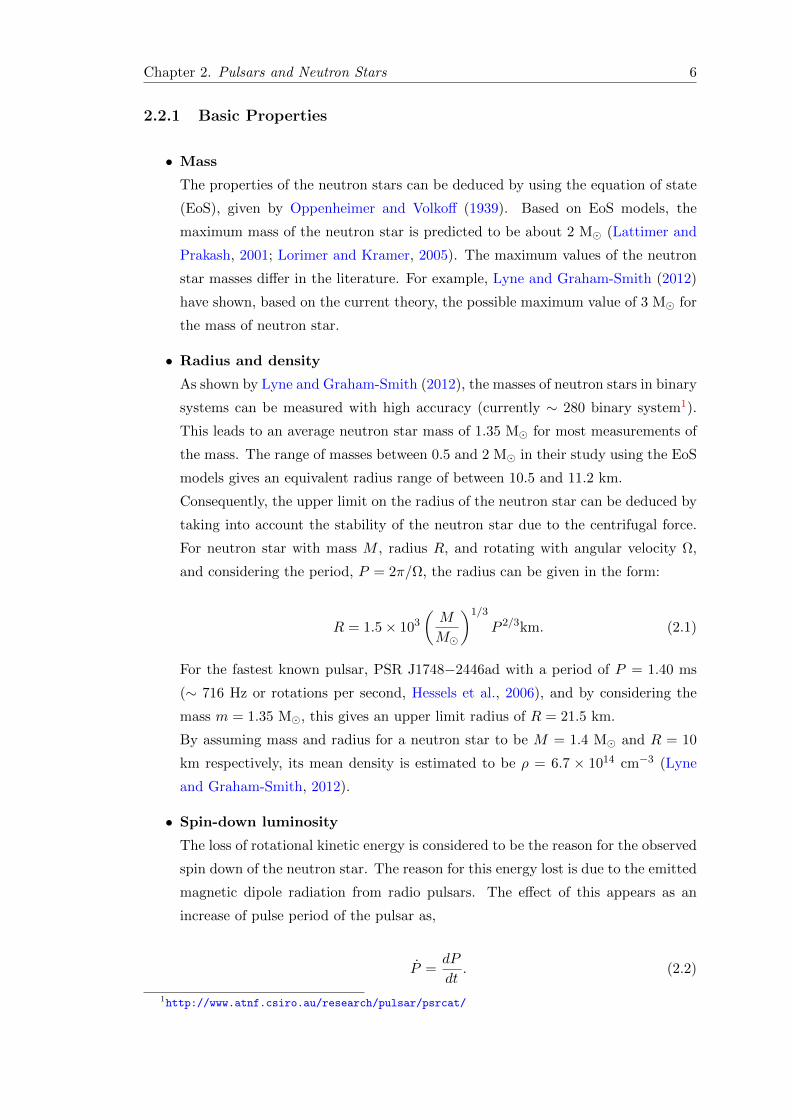
and escape through the open field lines (e.g. Figure 2.2).
Figure 2.2: Diagram presenting the Goldreich-Julian model. Showing the pulsarmagnetosphere that contains a polar gap with the electron-positron cascades. Figure
taken from Handbook of Pulsar Astronomy by Lorimer and Kramer (2005).
Following the model of Goldreich and Julian (1969), another attempt was carried out
by Sturrock (1971). He proposed a new model of “polar caps”. The polar caps are the
areas where the open field lines reach the light cylinder and connect with the surface of
the star in Figure 2.2. The electrons are accelerated along the open magnetic field lines
which leads to the production of a γ-ray emission due to the curvature radiation. If the
pulsar has a short period (P < 1 second), electron-positron pairs will be generated and
accelerated for the second time to produce more emission in the form of a pair cascade.
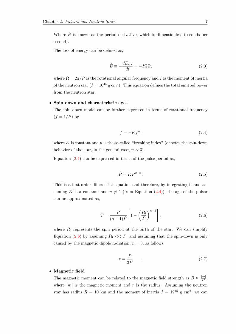
Ruderman and Sutherland (1975) proposed an improved model, the so-called “polar
Chapter 2. Pulsars and Neutron Stars 9
Figure 2.3: The rotating dipole of the pulsar emission of the polar gap model. Thepairs of electrons-positrons are accelerated through the “gap” regions of the magneto-sphere. The pairs then escape along the open magnetic fields lines to emit two beams ofradiation. Figure taken from Handbook of Pulsar Astronomy by Lorimer and Kramer
(2005).
gap” model, which expands on the previous model, by suggesting that the open field
lines are extended to a high altitude from the stellar surface by the polar magnetosphere
gap. This creates a potential difference of 1012 volts between the top and the base of
the gap, as a result, the gap “spark” by generating electron-positron pairs which in turn
are responsible for the emission (e.g. Figure 2.3).
2.2.3 The Galactic Distribution
The standard model of neutron star formation proposed that neutron stars are the result
of supernova explosions of the massive stars (Lyne and Lorimer, 1994). When a main
sequence star, with mass m ≥ 10 M, explodes, it leaves a stable core that is supported
against the gravitational collapse by so-called neutron degeneracy pressure (i.e. Type
II supernova) which gives birth to a neutron star. The newly created neutron star has
Chapter 2. Pulsars and Neutron Stars 10
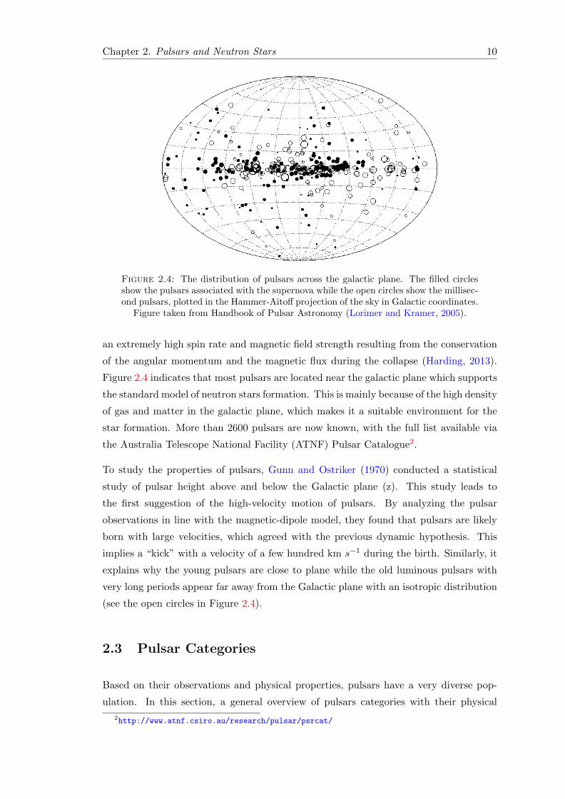
Figure 2.4: The distribution of pulsars across the galactic plane. The filled circlesshow the pulsars associated with the supernova while the open circles show the millisec-ond pulsars, plotted in the Hammer-Aitoff projection of the sky in Galactic coordinates.
Figure taken from Handbook of Pulsar Astronomy (Lorimer and Kramer, 2005).
an extremely high spin rate and magnetic field strength resulting from the conservation
of the angular momentum and the magnetic flux during the collapse (Harding, 2013).
Figure 2.4 indicates that most pulsars are located near the galactic plane which supports
the standard model of neutron stars formation. This is mainly because of the high density
of gas and matter in the galactic plane, which makes it a suitable environment for the
star formation. More than 2600 pulsars are now known, with the full list available via
the Australia Telescope National Facility (ATNF) Pulsar Catalogue2.
To study the properties of pulsars, Gunn and Ostriker (1970) conducted a statistical
study of pulsar height above and below the Galactic plane (z). This study leads to
the first suggestion of the high-velocity motion of pulsars. By analyzing the pulsar
observations in line with the magnetic-dipole model, they found that pulsars are likely
born with large velocities, which agreed with the previous dynamic hypothesis. This
implies a “kick” with a velocity of a few hundred km s−1 during the birth. Similarly, it
explains why the young pulsars are close to plane while the old luminous pulsars with
very long periods appear far away from the Galactic plane with an isotropic distribution
(see the open circles in Figure 2.4).
2.3 Pulsar Categories
Based on their observations and physical properties, pulsars have a very diverse pop-
ulation. In this section, a general overview of pulsars categories with their physical
2http://www.atnf.csiro.au/research/pulsar/psrcat/
Chapter 2. Pulsars and Neutron Stars 11
properties and evolution paths is given.
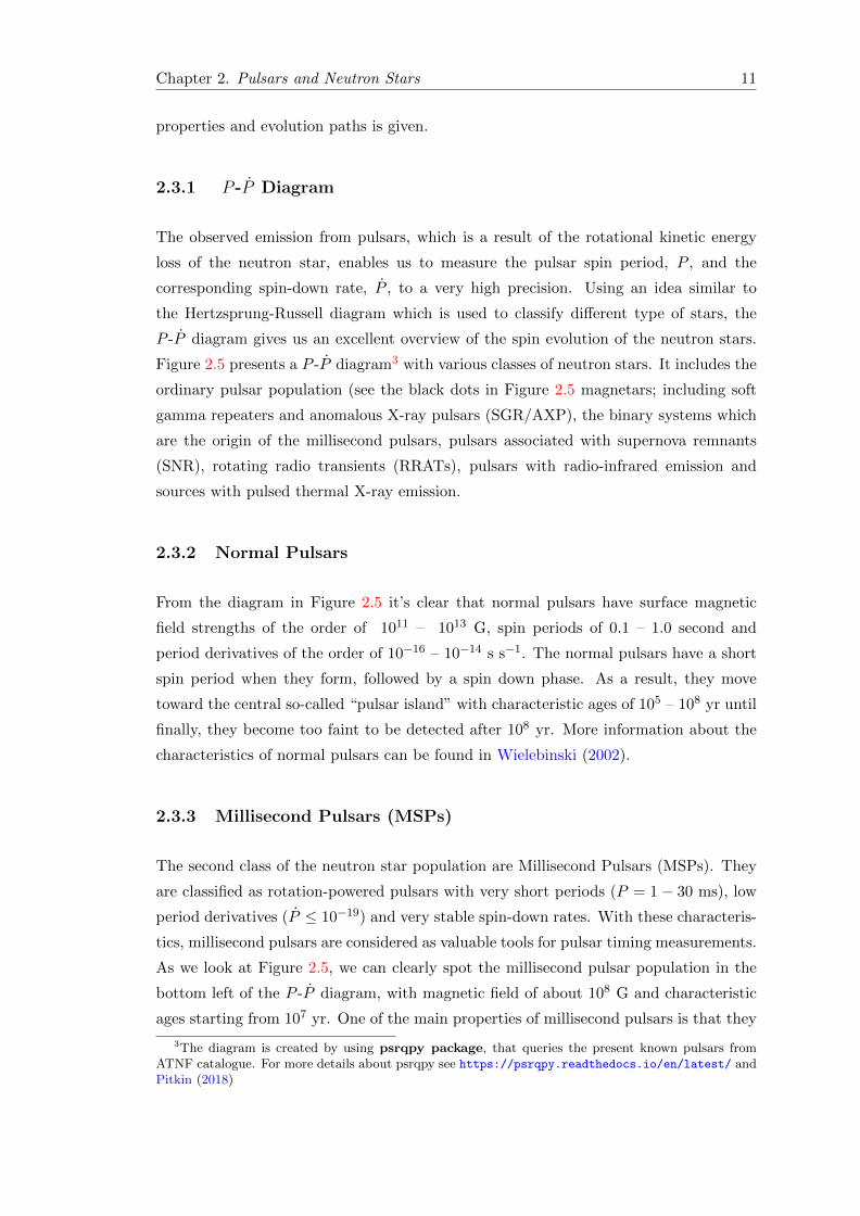
2.3.1 P -P Diagram
The observed emission from pulsars, which is a result of the rotational kinetic energy
loss of the neutron star, enables us to measure the pulsar spin period, P , and the
corresponding spin-down rate, P , to a very high precision. Using an idea similar to
the Hertzsprung-Russell diagram which is used to classify different type of stars, the
P -P diagram gives us an excellent overview of the spin evolution of the neutron stars.
Figure 2.5 presents a P -P diagram3 with various classes of neutron stars. It includes the
ordinary pulsar population (see the black dots in Figure 2.5 magnetars; including soft
gamma repeaters and anomalous X-ray pulsars (SGR/AXP), the binary systems which
are the origin of the millisecond pulsars, pulsars associated with supernova remnants
(SNR), rotating radio transients (RRATs), pulsars with radio-infrared emission and
sources with pulsed thermal X-ray emission.
2.3.2 Normal Pulsars
From the diagram in Figure 2.5 it’s clear that normal pulsars have surface magnetic
field strengths of the order of 1011 – 1013 G, spin periods of 0.1 – 1.0 second and
period derivatives of the order of 10−16 – 10−14 s s−1. The normal pulsars have a short
spin period when they form, followed by a spin down phase. As a result, they move
toward the central so-called “pulsar island” with characteristic ages of 105 – 108 yr until
finally, they become too faint to be detected after 108 yr. More information about the
characteristics of normal pulsars can be found in Wielebinski (2002).
2.3.3 Millisecond Pulsars (MSPs)
The second class of the neutron star population are Millisecond Pulsars (MSPs). They
are classified as rotation-powered pulsars with very short periods (P = 1− 30 ms), low
period derivatives (P ≤ 10−19) and very stable spin-down rates. With these characteris-
tics, millisecond pulsars are considered as valuable tools for pulsar timing measurements.
As we look at Figure 2.5, we can clearly spot the millisecond pulsar population in the
bottom left of the P -P diagram, with magnetic field of about 108 G and characteristic
ages starting from 107 yr. One of the main properties of millisecond pulsars is that they
3The diagram is created by using psrqpy package, that queries the present known pulsars fromATNF catalogue. For more details about psrqpy see https://psrqpy.readthedocs.io/en/latest/ andPitkin (2018)
Chapter 2. Pulsars and Neutron Stars 12
Figure 2.5: The P -P diagram for the currently known: Magneters (SGR/AXP);pulsars in binary system (Binary); pulsars with radio-infrared emission, radio-quietneutron stars; Rotating Radio Transients (RRATs); Radio-Quiet; Pulsed Themal X-ray and pulsars associated with supernova remnants (SNR) (from http://www.atnf.
csiro.au/people/pulsar/psrcat/). The diagram also include crossed lines which areused to determine the characteristic age (dot-dash lines) and the magnetic fields of the
population (dotted lines).
Chapter 2. Pulsars and Neutron Stars 13
have orbiting companions, observed in ∼ 80% of the total number of millisecond pulsars
(compared to ∼ 1% for the normal pulsars). These orbiting companions could be either
a main sequence star, a white dwarf or a neutron star.
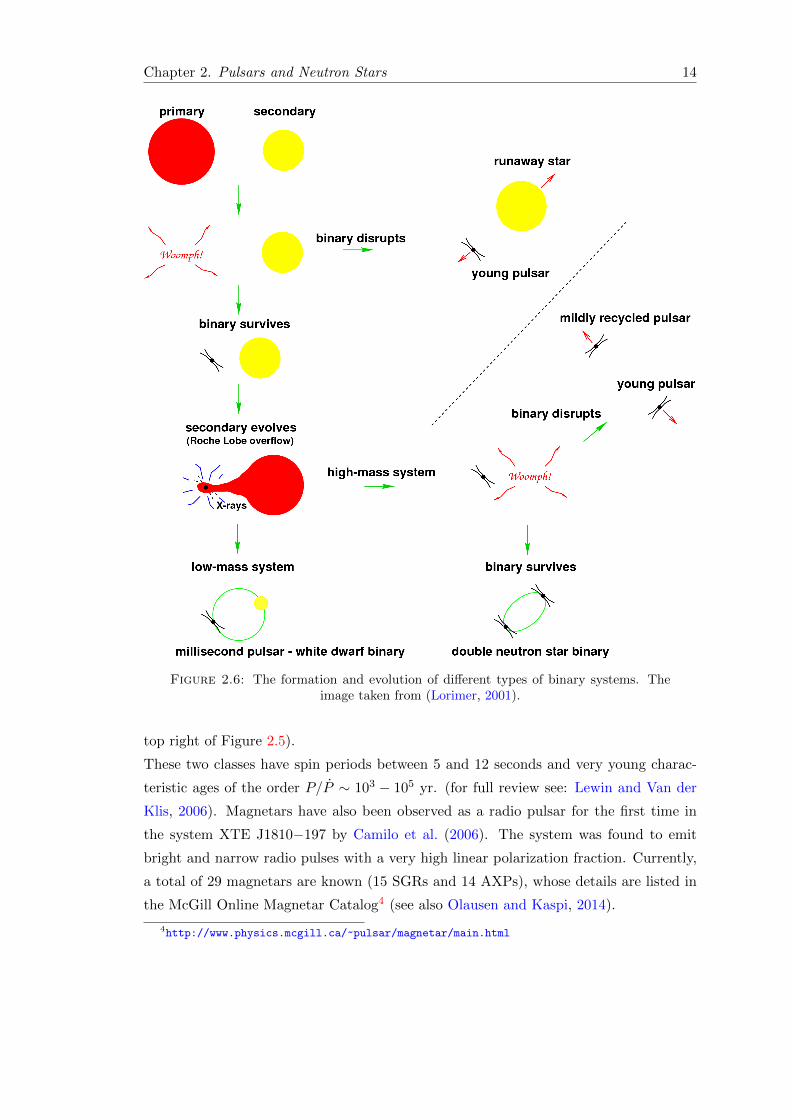
The formation and evolutionary model for different binaries is shown in Figure 2.6.
During the spin-down phase of pulsars in binary systems, they remain bound to the
companion. Then the companion starts to expand and evolve to become a giant star. As
a result, the distance between the pulsar and its companion will decrease which enables
the companion to fill its Roche Lobe and subsequently, transfer the orbital momentum
into the neutron star via an accretion disk. Next, the pulsar is spun up to a very short
rotation period. This process creates a millisecond pulsar with a very low slow-down
rate, so-called “recycled pulsar”. At this stage, the X-ray emission will commence and
the system is called an X-ray binary.
Depending on the mass of the companion, two classes can be identified: i) high-mass
X-ray binaries (HMXBs) and ii) low-mass X-ray binaries (LMXBs). In the case of the
HMXBs shown in Figure 2.6, if the binary is not disrupted in the process of the supernova
explosion, it will become a double neutron star (DNS, see bottom right part of Figure
2.6). Example of such a system is PSR B1913+16, which was reported by Taylor and
Weisberg (1982). The PSR J0737−3039 system (Burgay et al., 2003) is the first-known
double pulsar system where the two pulsars were observed with a period of 22 ms for A
and ∼ 2.8 s for B, and the orbital period between the two companions is equal to 2.4
hours. This makes it one of the best system to be used for testing the theory of general
relativity. HMXBs can also form a neutron star-black hole binary or even a black hole
binary, none of which has been discovered yet.
For the LMXBs case, the system evolves to be a millisecond pulsar-white dwarf binary
system. For a full review see (Lorimer, 2001 and Backer et al., 1982).
2.3.4 Magnetars
Magnetars are a type of neutron star with an ultra-high magnetic field (i.g. 1014 − 1016
Gauss). As suggested in the magnetar model by Duncan and Thompson (1992), the
decay of the magnetic field is the main source of the energy: “The magnetic fields can
deposit an enormous amount of energy outside a young neutron, and can catalyze the
conversion of energy from neutrinos to electron pairs”.
Depending on their observed emissions, two classes of magnetars are recognized: i) Soft
Gamma Repeaters (SGRs) which are identified as high-energy transient sources, and ii)
rapidly spinning Anomalous X-ray Pulsars (AXPs) which show continuing pulsation in
X-rays, with some of the sources exhibiting SGR-like bursts (denoted by red squares in
Chapter 2. Pulsars and Neutron Stars 14
Figure 2.6: The formation and evolution of different types of binary systems. Theimage taken from (Lorimer, 2001).
top right of Figure 2.5).
These two classes have spin periods between 5 and 12 seconds and very young charac-
teristic ages of the order P/P ∼ 103 − 105 yr. (for full review see: Lewin and Van der
Klis, 2006). Magnetars have also been observed as a radio pulsar for the first time in
the system XTE J1810−197 by Camilo et al. (2006). The system was found to emit
bright and narrow radio pulses with a very high linear polarization fraction. Currently,
a total of 29 magnetars are known (15 SGRs and 14 AXPs), whose details are listed in
the McGill Online Magnetar Catalog4 (see also Olausen and Kaspi, 2014).
4http://www.physics.mcgill.ca/~pulsar/magnetar/main.html
Chapter 2. Pulsars and Neutron Stars 15
2.3.5 Rotating Radio Transients (RRATs)
Another class of neutron star was identified as the Rotating Radio Transients (RRATs).
The discovery of RRATs was presented by McLaughlin et al. (2006). The authors
described eleven sources identified through their single pulses of radio emission using
data from the Parkes Multi-beam Pulsar Survey (PMPS) recorded between January 1998
and February 2002. The sources were characterized by short radio bursts of durations
between 2 and 30 ms. The average time intervals between bursts range between 4
minutes and 3 hours. Later, each source was re-observed and showed a number of pulses
(between 4 and 229 from each source with a period ranging from 0.4 to 7 second) and
renamed as Rotating Radio Transients (RRATs).
As appears in Figure 2.5, RRATs have characteristic age τ ≥ 107 yr (the green hexagons
shape at the top right of the figure). Currently, more than 100 sources are identified
including the recent discovery of 25 RRATs (see Tyul’bashev et al., 2018). For further
details see Keane (2010) and Harding (2013). The detailed properties of RRATs can be
found in the RRATalog5.
2.4 Interstellar Medium (ISM)
The interstellar medium (ISM) is the environment between the star systems in a galaxy
that contains ordinary matter, relativistic charged particles (cosmic rays) and magnetic
fields. The standard model consists of three components which are in pressure equi-
librium. Two of these components were suggested by Field et al. (1969) based on the
heating by low-energy cosmic rays. i) the cold dense phase, T < 300K, which consists
of neutral and molecular hydrogen clouds and ii) the warm intercloud phase, T = 104K,
consisting of ionized gas. The third phase is the hot ionized gas with a temperature of
T = 106K added by McKee and Ostriker (1977). Their study showed that the hot ion-
ized gas is a result of the supernova explosions which create shock-waves that evaporate
the cool clouds to a hot medium.
As the radio emission from pulsars propagates through the ionized interstellar medium
(IISM), it interacts with the free electrons, leading to observable propagation effects.
There are three main effects that can influence the pulsar signals while they travel
through the IISM: scintillation, scattering, and dispersion. In order to be able to observe
pulsars, one needs to correct for these effects (e.g. Armstrong et al., 1995).
5http://astro.phys.wvu.edu/rratalog/
Chapter 2. Pulsars and Neutron Stars 16
2.4.1 Dispersion
As was mentioned earlier, the dispersion of a pulsar signal is one of the important
characteristics of the ISM. The refractive index (n) of the ionized gas can be obtained
from the plasma frequency fp as follows,
n =
(1−
f2p
f2
)1/2
. (2.9)
Note that, the electron density, ne, in ISM environment is given in cm−3. As the
approximate value of ne = 0.03 cm−3 gives a plasma frequency, fp, of 1.5 kHz, then we
can approximate the refractivity (n − 1) to be −2.4 × 10⁻¹⁰ for a frequency, f , of 100
kHz. See Lyne and Graham-Smith (2012) for full explanation.
The plasma frequency in Equation (2.9) can be obtained as,
fp =
√nee2
πme' 8.5kHz(
necm−3
)1/2, (2.10)
where n is the refractive index of the ionized gas and f is the frequency of the wave, e
and m are the electronic charge and mass respectively. Since the group velocity of the
traveling pulses is νg = cn, where c is the speed of light in vacuum, thus for the given
electron densities, the group velocity is
ν2g = c
(1− nee
2
πmef2
). (2.11)
The travel time T through the distance L, therefore, will be in the form
T =
∫ L
0
dl
vg=L
c+e2∫ L
0 nedl
2πmcv2=L
c+ 1.345× 10⁻³v−2
∫ L
0nedl (2.12)
This equation shows the travel time in vacuum (the first term) with an additional term
which represents the dispersive delay t. The extra term contains the dispersion measure
(DM) given as follows,
DM =
∫ L
0nedl. (2.13)
The DM measures the electron density between the pulsar and the observer, with units
cm−3pc.

Chapter 2. Pulsars and Neutron Stars 17
From Equation (2.12) and (2.13), the delay due to dispersion can be written in the form,
t = D × DM
f2, (2.14)
where D is the dispersion constant which can be given as,
D =e2
4πmc= 4.1488× 10³MHz2pc−1cm3. (2.15)
If we have two different frequencies (flow and fhigh), then Equation (2.14) can be written
in another useful form as,
∆t = D ×DM ×
(1
f2low
− 1
f2high
). (2.16)
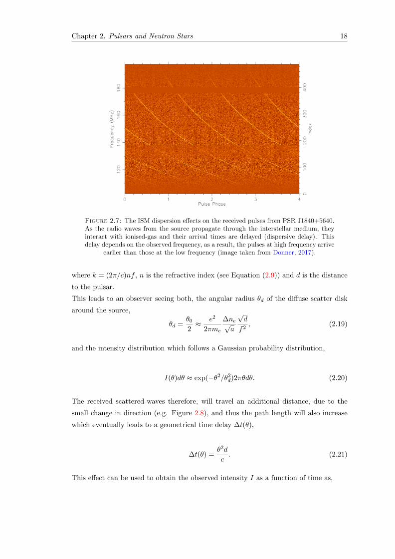
The effect of this delay can be seen in the observations when the pulses with higher
frequencies arrive earlier than those in low frequencies (e.g. Figure 2.7). The time
differences of the received signal with bandwidth B (in MHz) can be calculated (in
seconds) as
∆t = 8.3× 10³DMf2B (2.17)
2.4.2 Scattering
Another effect of the interstellar medium in pulsar signals is so-called scattering. The
inhomogeneities in the electron density along the line of sight scatter the radio pulses.
The combined effect of the inhomogeneities on the observed pulses is the broadening of
pulses in time. To characterize this effect, a simple model of a thin screen was proposed
by Williamson (1972), where the scattered radio waves along the line-of-sight from the
pulsars to an observer lead to frequency-dependent effects such as the pulse broadening,
(e.g. Figure 2.8).
As the wave propagates through an inhomogeneity (with scale a), its phases change due
to the refractive index and thus, by considering a screen midway between the pulsar and
the observer, we can identify this phase change ∆φ by approximating the angle θ0 at
the screen as,
θ0 ≈∆φ/k
a≈ e2
πme
∆ne√a
√D
f2, (2.18)
Chapter 2. Pulsars and Neutron Stars 18
Figure 2.7: The ISM dispersion effects on the received pulses from PSR J1840+5640.As the radio waves from the source propagate through the interstellar medium, theyinteract with ionised-gas and their arrival times are delayed (dispersive delay). Thisdelay depends on the observed frequency, as a result, the pulses at high frequency arrive
earlier than those at the low frequency (image taken from Donner, 2017).
where k = (2π/c)nf , n is the refractive index (see Equation (2.9)) and d is the distance
to the pulsar.
This leads to an observer seeing both, the angular radius θd of the diffuse scatter disk
around the source,
θd =θ0
2≈ e2
2πme
∆ne√a
√d
f2, (2.19)
and the intensity distribution which follows a Gaussian probability distribution,
I(θ)dθ ≈ exp(−θ2/θ2d)2πθdθ. (2.20)
The received scattered-waves therefore, will travel an additional distance, due to the
small change in direction (e.g. Figure 2.8), and thus the path length will also increase
which eventually leads to a geometrical time delay ∆t(θ),
∆t(θ) =θ2d
c. (2.21)
This effect can be used to obtain the observed intensity I as a function of time as,
Chapter 2. Pulsars and Neutron Stars 19
I(t) ≈ exp(−c∆t/(θ2dd)) ≡ e−∆t/τs , (2.22)
where
τs =θ2dd
c=
e4
4π2m2e
∆n2e
ad2f−4. (2.23)
This causes the observed scattering tail with the exponential shape that appears on the
received pulse signal.
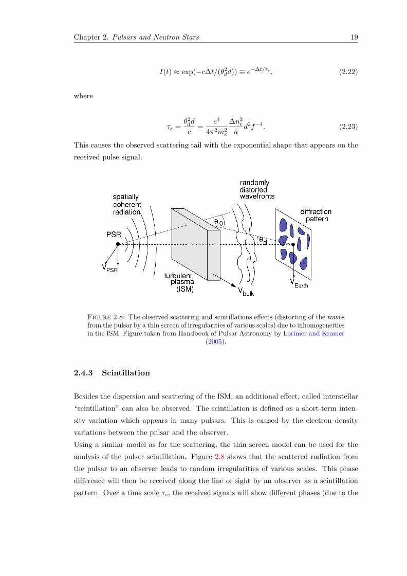
Figure 2.8: The observed scattering and scintillations effects (distorting of the wavesfrom the pulsar by a thin screen of irregularities of various scales) due to inhomogeneitiesin the ISM. Figure taken from Handbook of Pulsar Astronomy by Lorimer and Kramer
(2005).
2.4.3 Scintillation
Besides the dispersion and scattering of the ISM, an additional effect, called interstellar
“scintillation” can also be observed. The scintillation is defined as a short-term inten-
sity variation which appears in many pulsars. This is caused by the electron density
variations between the pulsar and the observer.
Using a similar model as for the scattering, the thin screen model can be used for the
analysis of the pulsar scintillation. Figure 2.8 shows that the scattered radiation from
the pulsar to an observer leads to random irregularities of various scales. This phase
difference will then be received along the line of sight by an observer as a scintillation
pattern. Over a time scale τs, the received signals will show different phases (due to the
Chapter 2. Pulsars and Neutron Stars 20
change in the intensity) as,
δΦ ∼ 2πfτs. (2.24)
The condition for interference to occur is when the phases of the waves do not differ
by more than 1 radian. Therefore the scintillation bandwidth (∆f) can be described as
follows,
2π∆fτs ∼ 1, (2.25)
which gives a scaling of ∆f ∝ 1/τs ∝ f4.
As the result, scintillation shows a pattern of intensity irregularities in both frequency
and time, which can be measured by producing a two-dimensional image as a function of
observed time and frequency called the dynamic spectrum. The regions of enhanced flux
density in these dynamic spectra are referred to as scintle. The scintle size in frequency
(scintillation bandwidth ∆f) and time (scintillation timescale ∆τ) can be measured as
the half-width at half-maximum of the auto-correlation function of the spectrum, and
the half-width at 1/e along the time axis respectively.
In the case where the ionized gas in the ISM is modeled as a turbulent gas, the variation
in electron density shows a distribution of scales, which is different from a single scale
size, a, as presented above. By changing from the single size to a distribution of length
scales which can be characterized by a spatial wavenumber spectrum, one can give a
better interpretation for the observations. The extended power law model can be used
as follows:
Pne(q) =C2ne
(z)
(q2 + k20)β/2
exp
[− q2
4k2i
], (2.26)
where q = 1/a is the magnitude of the three-dimensional wavenumber, ki and k0 are
the inner and the outer scales of the turbulence respectively, and C2ne
(z) represents the
strength of the fluctuations along the line of sight (for a full review on turbulence see
Rickett, 1990). Integrating the term C2ne
(z) along the line of sight gives the so-called
scattering measure (SM) as,
SM =
∫ d
0C2ne
(z)dz. (2.27)
Chapter 2. Pulsars and Neutron Stars 21
The scattering measure provides a measurement of the electron density fluctuations
along the line-of-sight and can be identified from the broadening of the average pulse
profile. In Equation (2.26), ki and ko are equal to the inner and outer cut-offs of scale
sizes. As mentioned earlier, these scales describe the scales distribution of the electron
density variations of the turbulent gas in the ISM. Considering wavenumber q between
ko q ki, Equation (2.26) can then be re-written as a power law model with spectral
index β as follows,
Pne(q) = C2neq−β. (2.28)
For the turbulent media, one can apply a Kolmogorov spectrum with β = 11/3. This
leads to frequency-dependence scattering time (τs) and decorrelation bandwidth (∆fDISS)
as follows,
τs ∝ f−α, ∆fDISS ∝ fα, (2.29)
where α = 2β/(β − 2), which gives α = 4.4 for a Kolmogorov spectrum (β = 11/3) and
α = 4 for the thin screen model. The term ∆fDISS is referred to diffractive interstellar
scintillation bandwidth. In Chapter 4, we will apply DM structure function analysis to
the resulted DM variations from the observations, which enable us to examine either
they show a compatible result with Kolmogorov spectrum or not.
2.5 Pulsar Timing
Pulsar timing is the measurement of a time-of-arrivals (TOAs) of pulses from the neutron
stars. These TOAs are computed by fitting the so-called timing model (see § 2.5.3) to
the observed time-of-arrival of pulses. As a result, the difference between the observed
and predicted arrival times gives the so-called timing residual. Study and analysing
of these residuals is considered the basis of all pulsar timing which can be obtained by
searching for correlation in the signals of the pulsar timing residuals (Hobbs, 2009).
Pulsar timing applications are ranging from studying the ISM properties, the mass of
the neutron stars, stellar evolution and searching for the stochastic gravitational waves
(GWs) background. Similarly, applying pulsar timing techniques on pulsars in a binary
system enables measurements of their orbits, rotation slowdown and testing Einstein’s
theory of General Relativity (GR).
Chapter 2. Pulsars and Neutron Stars 22
Multiple efforts were started to construct pulsar Timing Arrays to perform high-precision
pulsar timing using pulsar observations over a long time duration. These are three
sub-individual projects which are: European Pulsar Array (EPTA) in Europe, Parkes
Pulsar Timing Array (PPTA) in Australia and North American Nanohertz Observatory
for Gravitational Waves (NANOGrav) in the United States. As the main aim of PTAs is
to deliver a direct detection of the stochastic gravitational waves background, the data
from the three PTAs projects are being combined in the so-called International Pulsar
Timing Array (IPTA, e.g Hobbs et al., 2010, Verbiest et al., 2016).
The current and near future of pulsar timing is very promising. This is thanks to
the new instruments such as FAST telescope in China and MeerKAT in South Africa
which has been launched on Friday the 13th of July 2018. One of MeerKAT key science
programs in pulsar timing is MeerTIME (Bailes et al., 2018), which aims to observe over
1000 pulsars, during the period of five years, with the MeerKAT telescope in an efforts
to detect the stochastic gravitational waves (GW) background, study the interiors of
neutron stars, tests the relativistic theory of gravity and other topics related with pulsar
science.
In this section, an overview of pulsar timing techniques, TOAs and timing model and
its parameters are given. This section is based on Lorimer and Kramer (2005) and the
recent review by Manchester (2017).
2.5.1 Time of Arrivals (TOAs)
The time of arrival (TOA) is defined as “the arrival time of the nearest pulse to the mid-
point of the observation” Lorimer and Kramer (2005). In pulsar timing, the TOAs taken
from pulsars observations over long interval enable us to create a timing model; which
then can be used to determine the parameters of the pulsars, with a good accuracy, and
perform the analyses of their evolution. Practically, to measure the arrival times of the
pulses, the pulsars data need to be folded at the period of the pulsar. As a result, the
so-called “average pulse profile” will be created.
2.5.2 Template Matching
The cross-correlation method is considered the best method for measuring the timing
of arrival of pulsars (see Taylor, 1992). In this method, the observed profile is matched
with a high signal to noise (S/N) template. In our case, this template is constructed
from a set of earlier observations at a known range of frequencies.
By considering a scaled and shifted template T (t) with added noise N (t), the average
pulse profile P(t) then can be written as,
Chapter 2. Pulsars and Neutron Stars 23
P(t) = a+ bT (t− τ) +N (t), (2.30)
where a is the arbitrary offset, b is scaling factor and τ is the phase offset which shows
the time-shifted between the template and the profile. By applying the cross-correlation
between templates and the data (either in time domain or frequency domain), TOAs
can be measured.
The measurements of the TOAs can be done with high precision however, many effects,
either associated with the pulsars or as systematic effects, can limit it. This introduces
an uncertainty in the measurements of TOAs which can be calculated by the following
formula,
σTOA 'Ssys√tobs∆f
× Pδ3/2
Smean. (2.31)
Where Ssys is the flux density of the system, ∆f is the observed bandwidth, P is the
pulse period, tobs is the integration time, δ = W/P is the pulse duty cycle and the mean
flux density is given by Smean (Lorimer and Kramer, 2005).
2.5.3 Pulsar Timing-Model Parameters
In pulsar timing, the measured TOAs from the received pulses at the observatory need
to be fitted to a model by using an appropriate method (e.g cross-correlation 2.5.2).
Considering this fitting, there will be variations between the TOAs at the telescope and
the time of emission at the pulsar; hence, a timing model is required to correct all the
effects which limit our ability to measure the average TOAs with high accuracy.
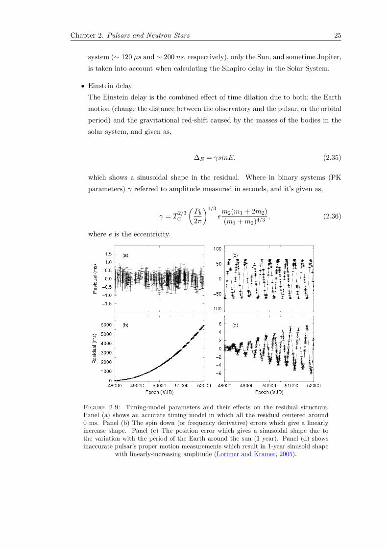
Here some of the parameters of the timing model and how they appear in the timing
residuals of the observations are discussed (e.g. Figure 2.9). For the full review see
Edwards et al. (2006).
• Barycentric corrections
Observatories on Earth measure the pulse TOAs by an atomic time standard called
“Terrestrial Time (TT)”; Measuring the TOAs using the observatory clock known
as “topocentric arrival time” which occurs in a non-inertial frame, due to rotating
Earth orbiting the Sun. Therefore, one needs to transfer this to an inertial reference
frame which represents the center of mass for the solar system. The frame of Solar
system barycenter (SSB) is approximated as a perfect inertial frame to measure
Chapter 2. Pulsars and Neutron Stars 24
the TOAs “barycentric arrival time”.
The transformation from the topocentric TOA to barycentric TOAs is given by
tSSB = ttopo + tcorr −∆D/f2 + ∆R + ∆S + ∆E . (2.32)
Equation (2.32) can be used as a reference to explain each term as follows:
• Clock corrections
The first two terms in Equation (2.32) ttopo and tcorr are corresponding to the time
measured by the observatory clock (topocentric time) and the observatory clock
corrections, respectively.
• Frequency corrections
∆D/f2 represents the dispersion measure and dispersion constant corrections. As
we showed in § 2.4.1 the pulses traveling through the ISM are delayed due to the
interaction with the ISM (dispersive delay), which shows that the TOAs depend
on the observed frequency (f).
• Romer delay
The term ∆R denotes the vacuum delay between the arrival of the pulse at the
observatory and SSB frame and can be given as,
∆R = −−→r .sc, (2.33)
where −→r is a vector pointing from the SSB frame toward the observatory, and
more precisely, can be divided to two components, −→r SSB which connect the SSB
with the center of the Earth (geo-centre) and −→r EO which connect the geo-center
with the phase center of the telescope. The second vector s in Equation (2.33) is
pointing from the SSB frame to the position of the pulsar.
• Shapiro delay
The Shapiro delay ∆S is a time delay of the pulses due to the curvature of space-
time. The total of this delay can be measured by adding all the masses in the solar
system as,
∆S = −2∑i
GMi
c3ln
[s.−→r Ei + rEis.−→r Pi + rPi
], (2.34)
where G is Newton gravitational constant, Mi is the mass of the included body
i, −→r Pi and −→r Ei are pulsar position and telescope position relative to the body i
respectively.
Note that, since the Sun and Jupiter have the largest Shapiro delay in the solar
Chapter 2. Pulsars and Neutron Stars 25
system (∼ 120 µs and ∼ 200 ns, respectively), only the Sun, and sometime Jupiter,
is taken into account when calculating the Shapiro delay in the Solar System.
• Einstein delay
The Einstein delay is the combined effect of time dilation due to both; the Earth
motion (change the distance between the observatory and the pulsar, or the orbital
period) and the gravitational red-shift caused by the masses of the bodies in the
solar system, and given as,
∆E = γsinE, (2.35)
which shows a sinusoidal shape in the residual. Where in binary systems (PK
parameters) γ referred to amplitude measured in seconds, and it’s given as,
γ = T2/3
(Pb2π
)1/3
em2(m1 + 2m2)
(m1 +m2)4/3, (2.36)
where e is the eccentricity.
Figure 2.9: Timing-model parameters and their effects on the residual structure.Panel (a) shows an accurate timing model in which all the residual centered around0 ms. Panel (b) The spin down (or frequency derivative) errors which give a linearlyincrease shape. Panel (c) The position error which gives a sinusoidal shape due tothe variation with the period of the Earth around the sun (1 year). Panel (d) showsinaccurate pulsar’s proper motion measurements which result in 1-year sinusoid shape
with linearly-increasing amplitude (Lorimer and Kramer, 2005).
Chapter 3
Observations and Data Reduction
The data used in this thesis were collected with the LOw-Frequency ARray (LOFAR)
telescope. Specifically, the observations were performed with international LOFAR sta-
tions: the Nancay station (FR606) in France, the Onsala station (SE607) in Sweden and
stations in Germany (DE601 - Effelsberg, DE602 - Unterweilenbach, DE603 - Tauten-
burg, DE605 - Julich). In this chapter, a general overview of the LOFAR telescope is
given in § 3.1 and a full description of the observations used in this study are given in
§ 3.2. In § 3.3 the data reduction process is explained.
3.1 LOw Frequency ARray (LOFAR)
The LOw-Frequency ARray (LOFAR, van Haarlem et al., 2013) is a unique radio tele-
scope that contains a number of interferometric arrays of dipole antenna stations spread
throughout Europe. LOFAR was designed and developed by the Netherlands Institute
for Radio Astronomy (ASTRON)1. It operates within the low-frequency regime of the
radio wavelengths, which is divided into low band (10 - 90 MHz) and high band (110 -
240 MHz). The range of these frequencies corresponds to wavelengths between 30 and
1.2 m. Additionally, LOFAR has a large field-of-view (FoV), which makes it an excellent
instrument for many key science projects such as surveying the low-frequency sky, the
transient radio sky and conducting pulsar studies and surveys. More details about the
pulsar key science projects are described in Stappers et al. (2011).
LOFAR telescope comprises of 38 stations in the Netherlands and thirteen international
stations distributed within the European partner countries (e.g. Figure 3.1). The in-
ternational stations are located in France, Germany, Ireland, Poland, Sweden and the
1https://www.astron.nl/
26
Chapter 3. Observations and Data Reduction 27
United Kingdom. Recently, Austria,Ukraine and Italy have joined the International
LOFAR Telescope (ITL2) with intentions to construct their own LOFAR stations. In
Finland, the Kilpisjarvi Atmospheric Imaging Receiver Array (KAIRA) makes use of
LOFAR antennas and digital signal-processing hardware but operates it as a stand-
alone instrument (McKay-Bukowski et al. 2015).
Similar to the individual antennas in interferometric radio telescopes such as MeerKAT
and the VLA, LOFAR stations can also perform the same basic functions e.g. track-
ing sources by combining the signals from individual antenna elements to form the
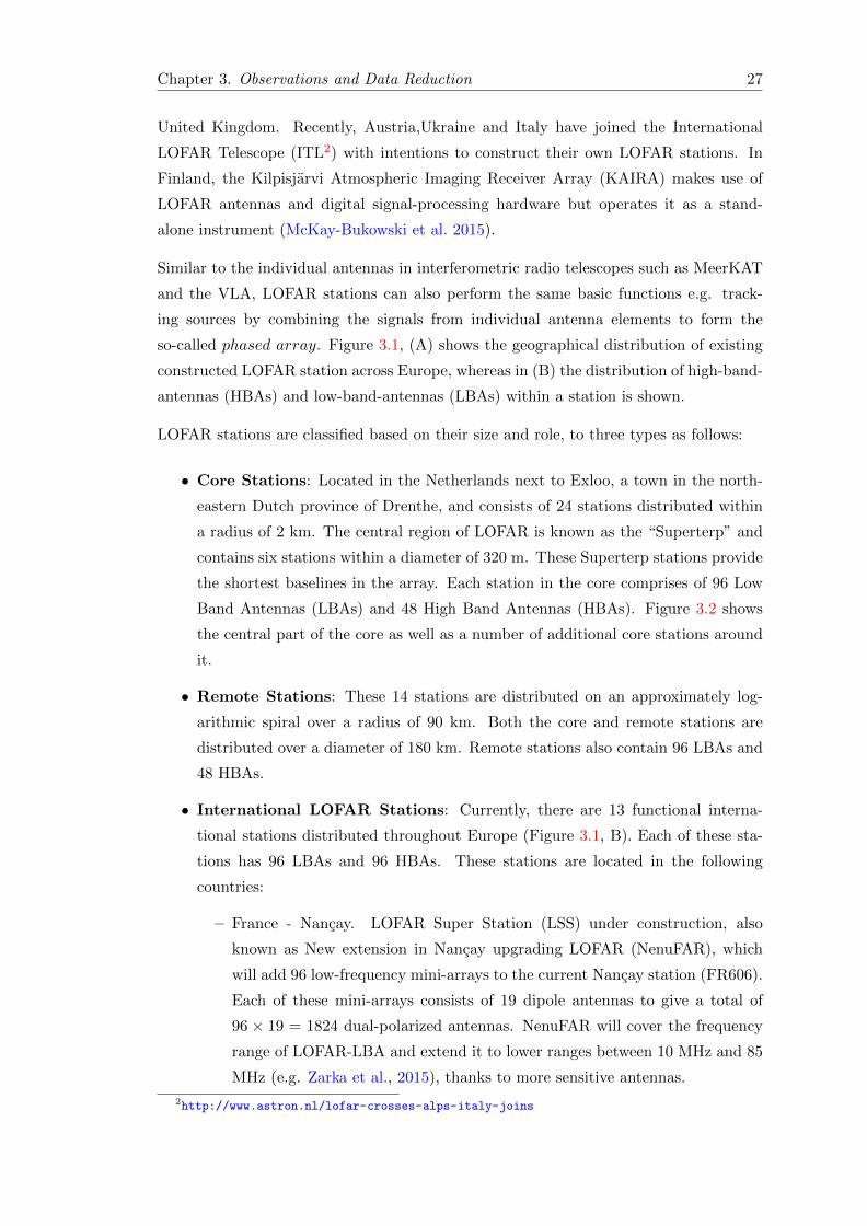
so-called phased array. Figure 3.1, (A) shows the geographical distribution of existing
constructed LOFAR station across Europe, whereas in (B) the distribution of high-band-
antennas (HBAs) and low-band-antennas (LBAs) within a station is shown.
LOFAR stations are classified based on their size and role, to three types as follows:
• Core Stations: Located in the Netherlands next to Exloo, a town in the north-
eastern Dutch province of Drenthe, and consists of 24 stations distributed within
a radius of 2 km. The central region of LOFAR is known as the “Superterp” and
contains six stations within a diameter of 320 m. These Superterp stations provide
the shortest baselines in the array. Each station in the core comprises of 96 Low
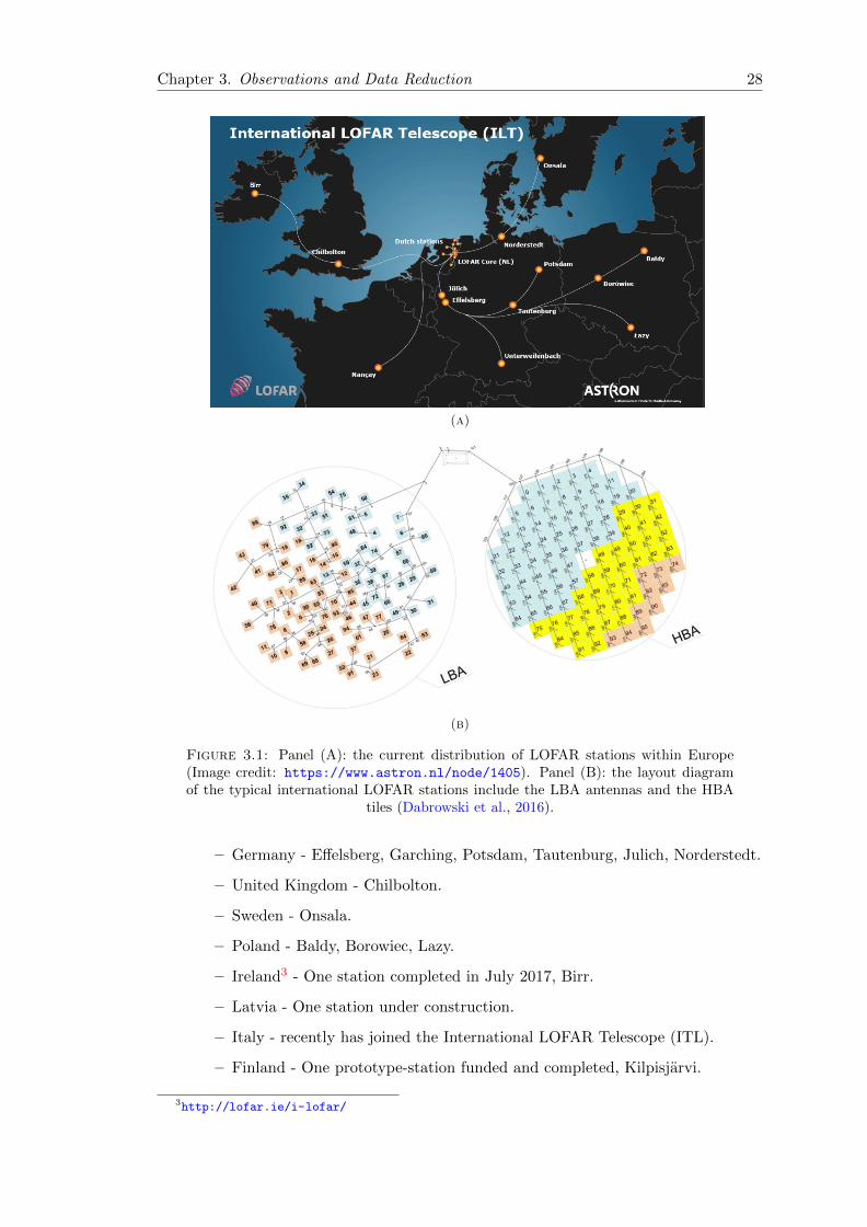
Band Antennas (LBAs) and 48 High Band Antennas (HBAs). Figure 3.2 shows
the central part of the core as well as a number of additional core stations around
it.
• Remote Stations: These 14 stations are distributed on an approximately log-
arithmic spiral over a radius of 90 km. Both the core and remote stations are
distributed over a diameter of 180 km. Remote stations also contain 96 LBAs and
48 HBAs.
• International LOFAR Stations: Currently, there are 13 functional interna-
tional stations distributed throughout Europe (Figure 3.1, B). Each of these sta-
tions has 96 LBAs and 96 HBAs. These stations are located in the following
countries:
– France - Nancay. LOFAR Super Station (LSS) under construction, also
known as New extension in Nancay upgrading LOFAR (NenuFAR), which
will add 96 low-frequency mini-arrays to the current Nancay station (FR606).
Each of these mini-arrays consists of 19 dipole antennas to give a total of
96 × 19 = 1824 dual-polarized antennas. NenuFAR will cover the frequency
range of LOFAR-LBA and extend it to lower ranges between 10 MHz and 85
MHz (e.g. Zarka et al., 2015), thanks to more sensitive antennas.
2http://www.astron.nl/lofar-crosses-alps-italy-joins
Chapter 3. Observations and Data Reduction 28
(a)
(b)
Figure 3.1: Panel (A): the current distribution of LOFAR stations within Europe(Image credit: https://www.astron.nl/node/1405). Panel (B): the layout diagramof the typical international LOFAR stations include the LBA antennas and the HBA
tiles (Dabrowski et al., 2016).
– Germany - Effelsberg, Garching, Potsdam, Tautenburg, Julich, Norderstedt.
– United Kingdom - Chilbolton.
– Sweden - Onsala.
– Poland - Baldy, Borowiec, Lazy.
– Ireland3 - One station completed in July 2017, Birr.
– Latvia - One station under construction.
– Italy - recently has joined the International LOFAR Telescope (ITL).
– Finland - One prototype-station funded and completed, Kilpisjarvi.
3http://lofar.ie/i-lofar/
Chapter 3. Observations and Data Reduction 29
(a) Superterp
(b) SE607 Station
Figure 3.2: (A) Aerial view of part of LOFAR with the Superterp in the middle(van Haarlem et al., 2013). (B) The image of Swedish LOFAR station in Onsala SpaceObservatory. The LBA antennas are located at the left side of the photo, while HBAtiles are clustered together in the right side. The station digital back-end (contains thedigital receiver units (RCUs), digital signal processing (DSP), local control unit (LCU),remote station processing (RSP)) are located in the container visible in the top center
of the photo. Credit: Onsala Space Observatory/Leif Helldner.
Chapter 3. Observations and Data Reduction 30
All LOFAR stations consist of two types of antennas described below:
• Low-Band Antenna (LBA)
The low-band antenna covers a frequency range between 10 MHz and 90 MHz. It
consists of dipole elements, each of which has a length of 1.38 m and is sensitive
to two orthogonal linear polarizations. There are 96 low-band antenna elements in
an international station, which are used as a single antenna array. Both, the core
and remote stations consist of 98 LBAs arranged in a single 87 m diameter field.
• High Band Antenna (HBA)
The high-band antenna covers a frequency range from 110 MHz to 240 MHz. 16
HBAs antenna elements (dual polarized) are clustered and phased to create a single
tile. Each of these tiles contains an analogue beamformer and low-noise amplifier
able to create a single “tile beam” for any given direction in the sky. The number
and distribution of HBA tiles are different in the three types of LOFAR stations.
While the international station consists of a single array of 96 tiles, remote station
consists of 48 HBAs arranged in a single 41 m diameter and the core station consists
of 48 HBAs arranged in two 24-elements fields where each field has a diameter of
30.8 m.
Signal processing with LOFAR
Each LOFAR station has a cabinet that contains receiver units (RCUs), digital signal
processing (DSP) boards, a local control unit (LCU), and other additional equipment
which are used to process the signals at the early stages. A brief description of data
processing in LOFAR can be given as follows: after receiving the signals at the LBA
elements or HBA tiles, they are transferred to the RCUs via coaxial cables. The RCUs
performs filtering, amplification, conversion to base-band frequencies and digitization of
the input signal. Subsequently, the received signals enter the remote station processing
boards (RSPs) for all the digital signal processing. In the RSPs, the signals are first
buffered to remove the differences in signal delays in the coaxial cables. Then, the
signals are filtered into 512 sub-bands by a polyphase filter. Based on the sample clock
frequency, the sub-bandwidth can be 195.312 kHz (200 MHz clock) or 156.250 kHz (160
MHz clock). The station beam is produced by RSP boards and the resulting product
is divided into four separate lanes. These lanes are then streamed to either a local
processing backend or to the central processor (CEP) in Groningen.
In addition to a RCU and DSP, as mentioned before each LOFAR station contains a local
control unit (LCU). This unit consists of a server computer running a Linux operating
system, which is used to control the station. Additionally, LCU receives clock signals
from the Global Positioning System (GPS) and a rubidium standard.
Chapter 3. Observations and Data Reduction 31
3.2 Observations
The observations used in this thesis are part of a long-term running observing proposal
(LC0 - 014, LC1 - 048, LC2 - 011, LC3 - 029, LC4 - 025, LT5 - 001, LC9 - 039 and
LT10 - 014, PI: Serylak) that aims to observe known pulsars with international LOFAR
stations, monitoring them with a weekly cadence where each observing session lasts
approximately one hour per target. A total number of 95 sources were selected and
monitored, this includes 14 millisecond pulsars and 81 slow pulsars, 5 of which were
discovered as part of the LOFAR Tied-Array All-Sky Survey4 (LOTAAS, Coenen et al.,
2014).
In this thesis, 27 sources from the running observing proposal were not included, due
to e.g. insufficient signal to noise ratio (SNR) or the number of observations, exclud-
ing all the millisecond pulsars, which reduced the total number of used sources to 68.
This includes only slow pulsars and 3 of the LOTAAS and LOFAR Tied-Array Survey5
(LOTAS, Coenen et al., 2014) discovered sources. In the analysis stage, observations in
the period roughly between June 2014 and November 2017 were used. Each observation
was performed for at least one hour (except PSR J0332+5434 which has 30 minutes ob-
servations) but not longer than two hours, in order for a pulsar to achieve the required
SNR.
All the observations were taken with HBAs, in the frequency range between 110 to
190 MHz. The data were recorded by LOFAR and MPIfR Pulsare (LuMP) Software6.
This software is used for recording beamformed data from a LOFAR station in the
single-station mode. All the data in this study are coherently dedispersed to remove
the possible dispersion smearing within specific frequency channels. In the following
sub-sections, I give an overview of the international LOFAR stations which are used to
obtain the data.
3.2.1 Observations with French Station (FR606)
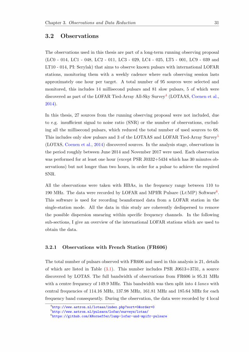
The total number of pulsars observed with FR606 and used in this analysis is 21, details
of which are listed in Table (3.1). This number includes PSR J0613+3731, a source
discovered by LOTAS. The full bandwidth of observations from FR606 is 95.31 MHz
with a centre frequency of 149.9 MHz. This bandwidth was then split into 4 lanes with
central frequencies of 114.16 MHz, 137.98 MHz, 161.81 MHz and 185.64 MHz for each
frequency band consequently. During the observation, the data were recorded by 4 local
4http://www.astron.nl/lotaas/index.php?sort=0&order=05http://www.astron.nl/pulsars/lofar/surveys/lotas/6https://github.com/AHorneffer/lump-lofar-und-mpifr-pulsare
Chapter 3. Observations and Data Reduction 32
Table 3.1: The initial parameters for the total number of pulsars fromFR606. These parameters are PSR B (based on B1950 designation), PSRJ (based on J2000 designation), pulse period (P), dispersion measurevalue (DM). The table is obtained using Australia Telescope National
Facility (ATNF) Pulsar Catalog (Manchester et al., 2005).
# PSR B PSR J PulsePeriod(s)
DM(cm−3pc)
1 B0138+59 J0141+6009 1.222 34.9262 B0320+39 J0323+3944 3.032 26.1893 B0329+54 J0332+5434 0.714 26.7644 B0450+55 J0454+5543 0.340 14.5905 B0540+23 J0543+2329 0.245 77.702
6 - J0613+3731** 0.619 18.9907 B0809+74 J0814+7429 1.292 5.7508 B0834+06 J0837+0610 1.273 12.8649 B0950+08 J0953+0755 0.253 2.969
10 B1133+16 J1136+1551 1.187 4.84011 B1237+25 J1239+2453 1.382 9.25112 B1508+55 J1509+5531 0.739 19.61913 B1540−06 J1543−0620 0.709 18.37714 B1642−03 J1645−0317 0.387 35.75515 B1737+13 J1740+1311 0.803 48.66816 B1822−09 J1825−0935 0.769 19.38317 B1931+24 J1933+2421 0.813 106.0318 B2016+28 J2018+2839 0.557 14.19719 B2111+46 J2113+4644 1.014 141.2620 B2224+65 J2225+6535 0.682 36.44321 B2310+42 J2313+4253 0.349 17.276
** LOTAS discovery
backends, to a large volume storage. All the observations with less than four parts of
the frequency bands were excluded from the study.
3.2.2 Observations with Swedish Station (SE607)
The Swedish LOFAR station7 is located at Onsala Space Observatory. The configuration
of this station is identical to that of the French Station (FR606). A total of 13 pulsars
from the SE607 station was used in this study. Table (3.2) displays all pulsars observed
with the station including the LOTAAS discovered pulsar, PSR J0815+4611. These
observations have the same properties as the data from FR606 (e.g. central-frequency,
number of channels, bandwidth etc.) and therefore, a similar approach was used during
data reduction steps (see § 3.3).
7http://www.chalmers.se/en/researchinfrastructure/oso/radio-astronomy/lofar/Pages/
default.aspx

Chapter 3. Observations and Data Reduction 33
Table 3.2: The initial parameters for the total number of pulsars fromSE607. These parameters are PSR B (based on B1950 designation),PSR J (based on J2000 designation), pulse period (P), dispersion mea-sure value (DM). All the samples were obtained using Australia TelescopeNational Facility (ATNF) Pulsar Catalog (Manchester et al., 2005) ex-cept J0815+4611 which is LOTAAS discovery and its parameters were
obtained from the initial ephemeris.
# PSR B PSR J PulsePeriod(s)
DM(cm−3pc)
1 - J0051+0423 0.354 13.92 B0059+65 J0102+6537 1.679 65.8533 B0331+45 J0335+4555 0.269 47.1454 - J0540+3207 0.524 61.975 - J0546+2441 2.843 73.816 B0655+64 J0700+6418 0.195 8.773
7 - J0815+4611** 0.434 11.278 B0917+63 J0921+6254 1.567 13.1549 B1112+50 J1115+5030 1.656 9.186
10 B1322+83 J1321+8323 0.67 13.31611 B1839+56 J1840+5640 1.652 26.77112 B1953+50 J1955+5059 0.518 31.98213 B2319+60 J2321+6024 2.256 94.591
** LOTAAS discovery
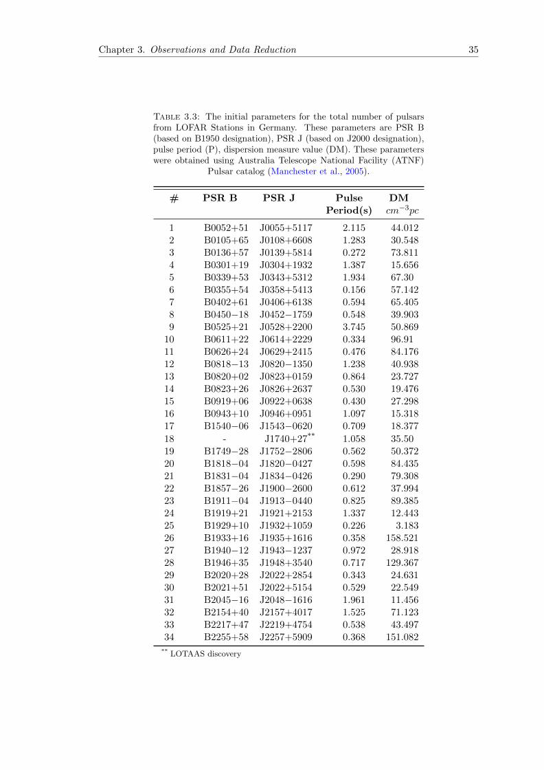
3.2.3 Observations with the LOFAR Stations in Germany
As mentioned earlier, there are 6 international stations located in Germany and operated
by the German LOng Wavelength (GLOW)8 group, which is a consortium formed by a
number of German universities and research institutes.
A set of 34 sources was obtained from four stations, namely DE601, DE602, DE603
and DE605. As opposed to the sources observed by FR606 or SE607, each source was
observed with more than one German station throughout 3.5 years of monitoring. Table
(3.3) shows all the data obtained from LOFAR stations in Germany.
The observations made with German stations have relatively longer observation spans
due to sources with weaker SNRs. Two sets of German station data were used which
include: i) early observations starting from mid August 2013 which have a total band-
width of 95.31 MHz and centre frequency 149.9 MHz. Each observation, using the full
bandwidth, was divided into four lanes, where each lane has 122 frequency channels,
1024 number of pulse phase bins and a lane width of 23.828 MHz. ii) later observations
which started in February 2015. In order to reduce the data rate for all German stations
8https://www.glowconsortium.de/index.php/en/
Chapter 3. Observations and Data Reduction 34
(except DE601 which consists of 4 lanes), the outer parts of the band, where the instru-
mental sensitivity is very low, were removed and as a result, the total bandwidth was
reduced to 71.484 MHz with a centre frequency of 153.808 MHz. The full bandwidth
was then divided into three lanes with 122 frequency channels, 1024 number of pulse
phase bin, and center frequency of 23.828 MHz for each. Additionally, the observations
with large differences in their number of the sub-integrations were rejected from the
reduction.
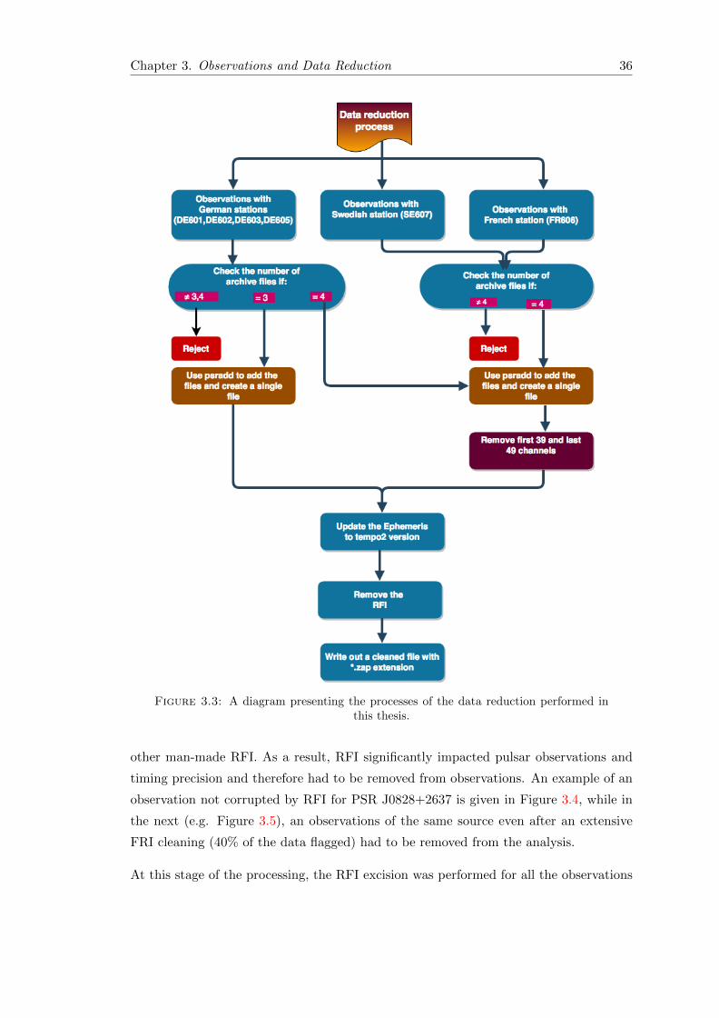
3.3 Data Reduction
Data reduction was performed using the readily available pulsar reduction package
psrchive9 (Hotan et al., 2004). In order to manage the reduction, python scripts
were prepared to operate the required tasks. These include updating the ephemeris and
performing radio frequency interference (RFI) excision. Additionally, bash scripts were
also prepared and used to perform tasks such as, creating diagnostic plots and produc-
ing final reports summarizing the reduction process. With the intention to decrease the
processing time, the data reduction was parallelized. This, in turn, allowed to complete
the data reduction in the shortest possible time (See Figure 3.3).
3.3.1 Data Processing
The first step of data reduction involved sorting the observations based on a number
of frequency channels and number of sub-integrations. Then, all the archives for each
observation were added to form a single file covering the bandwidth (488 frequency
channels for FR606 and SE607 and 366 frequency channels for the German stations).
In the following step, the resulting files were adjusted by removing edges of the band
where antennas were not sensitive. This was implemented by removing the first 39
and last 49 frequency channels creating an archive file with 400 frequency channels.
This procedure was performed for all observations taken with the FR606 and SE607
stations, as well as early observations performed with the German stations. No channel
removal was applied for the recent observations with German stations (three lanes) and
therefore, the number of the frequency channels was kept to be 366. At this stage, the
ephemeris of the archives were checked for uniformity and updated to a common version
if discrepancies were found.
As mentioned earlier, all observations were taken within the low-frequency band of
HBA antenna and close to the FM band (ranging between 87.5 MHz and 108 MHz) and
9http://psrchive.sourceforge.net/
Chapter 3. Observations and Data Reduction 35
Table 3.3: The initial parameters for the total number of pulsarsfrom LOFAR Stations in Germany. These parameters are PSR B(based on B1950 designation), PSR J (based on J2000 designation),pulse period (P), dispersion measure value (DM). These parameterswere obtained using Australia Telescope National Facility (ATNF)
Pulsar catalog (Manchester et al., 2005).
# PSR B PSR J PulsePeriod(s)
DMcm−3pc
1 B0052+51 J0055+5117 2.115 44.0122 B0105+65 J0108+6608 1.283 30.5483 B0136+57 J0139+5814 0.272 73.8114 B0301+19 J0304+1932 1.387 15.6565 B0339+53 J0343+5312 1.934 67.306 B0355+54 J0358+5413 0.156 57.1427 B0402+61 J0406+6138 0.594 65.4058 B0450−18 J0452−1759 0.548 39.9039 B0525+21 J0528+2200 3.745 50.869
10 B0611+22 J0614+2229 0.334 96.9111 B0626+24 J0629+2415 0.476 84.17612 B0818−13 J0820−1350 1.238 40.93813 B0820+02 J0823+0159 0.864 23.72714 B0823+26 J0826+2637 0.530 19.47615 B0919+06 J0922+0638 0.430 27.29816 B0943+10 J0946+0951 1.097 15.31817 B1540−06 J1543−0620 0.709 18.377
18 - J1740+27** 1.058 35.5019 B1749−28 J1752−2806 0.562 50.37220 B1818−04 J1820−0427 0.598 84.43521 B1831−04 J1834−0426 0.290 79.30822 B1857−26 J1900−2600 0.612 37.99423 B1911−04 J1913−0440 0.825 89.38524 B1919+21 J1921+2153 1.337 12.44325 B1929+10 J1932+1059 0.226 3.18326 B1933+16 J1935+1616 0.358 158.52127 B1940−12 J1943−1237 0.972 28.91828 B1946+35 J1948+3540 0.717 129.36729 B2020+28 J2022+2854 0.343 24.63130 B2021+51 J2022+5154 0.529 22.54931 B2045−16 J2048−1616 1.961 11.45632 B2154+40 J2157+4017 1.525 71.12333 B2217+47 J2219+4754 0.538 43.49734 B2255+58 J2257+5909 0.368 151.082
** LOTAAS discovery
Chapter 3. Observations and Data Reduction 36
Figure 3.3: A diagram presenting the processes of the data reduction performed inthis thesis.
other man-made RFI. As a result, RFI significantly impacted pulsar observations and
timing precision and therefore had to be removed from observations. An example of an
observation not corrupted by RFI for PSR J0828+2637 is given in Figure 3.4, while in
the next (e.g. Figure 3.5), an observations of the same source even after an extensive
FRI cleaning (40% of the data flagged) had to be removed from the analysis.
At this stage of the processing, the RFI excision was performed for all the observations
Chapter 3. Observations and Data Reduction 37
included in the study by using Surgical cleaner which is part of the Coastguard10
tool (Lazarus et al., 2016). Implementing aforementioned cleaning strategy on all ob-
servations allowed me to identify and remove those parts of the data corrupted by the
RFI. Coastguard has a set of parameters and settings which can be adjusted if the
initial processing does not give a satisfactory result.
In this study, I faced many challenges associated with RFI impacting the quality of
the data. In order to asses the quality of the reduced data, I prepared a diagnostic
report to inspect each observation (e.g. Figure 3.4). It contains numerical values such
as the amount of RFI removed from an observation, observational parameters, SNR etc.
The report also contains a number of diagnostic plots for visual inspection i.e. a sub-
integration stack, average profile, frequency profile, dynamic spectrum, and bandpass.
The average number of observations is roughly 160 per pulsar, where an average of 28
observations were rejected due to many reasons e.g. RFI, insufficient bandwidth etc.
10https://github.com/plazar/coast_guard
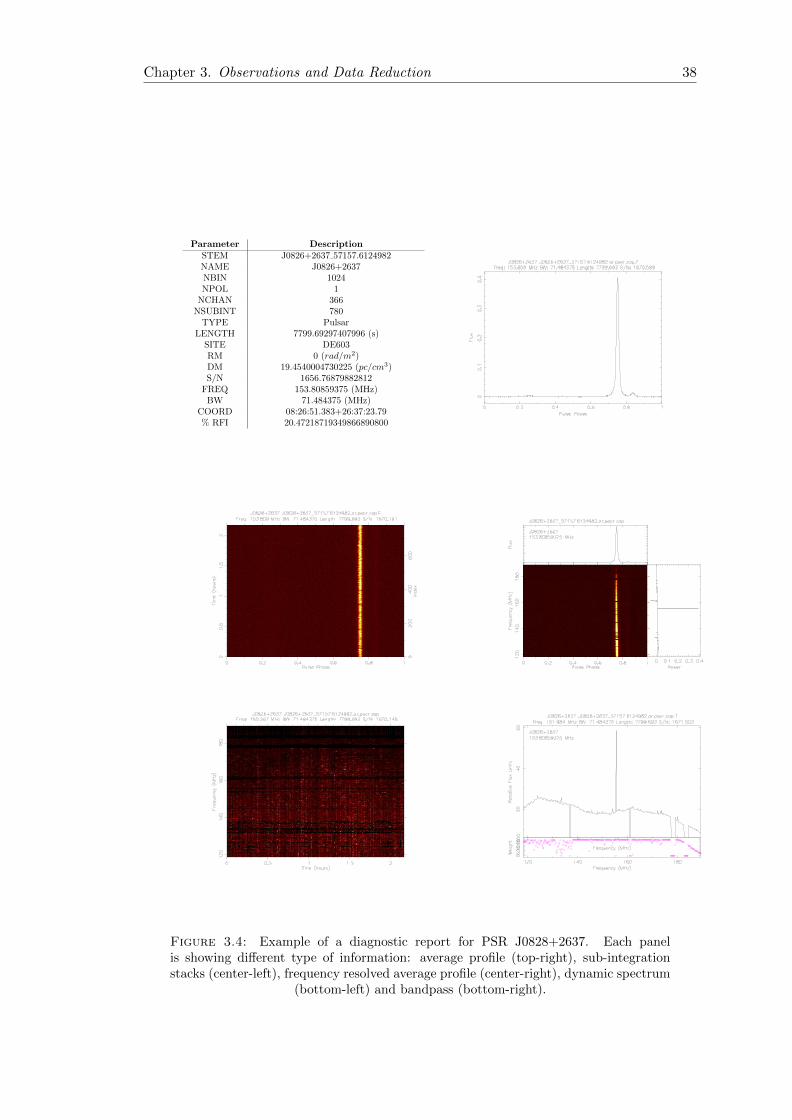
Chapter 3. Observations and Data Reduction 38
Parameter Description
STEM J0826+2637 57157.6124982NAME J0826+2637NBIN 1024NPOL 1
NCHAN 366NSUBINT 780
TYPE PulsarLENGTH 7799.69297407996 (s)
SITE DE603RM 0 (rad/m2)DM 19.4540004730225 (pc/cm3)S/N 1656.76879882812
FREQ 153.80859375 (MHz)BW 71.484375 (MHz)
COORD 08:26:51.383+26:37:23.79% RFI 20.47218719349866890800
Figure 3.4: Example of a diagnostic report for PSR J0828+2637. Each panelis showing different type of information: average profile (top-right), sub-integrationstacks (center-left), frequency resolved average profile (center-right), dynamic spectrum
(bottom-left) and bandpass (bottom-right).
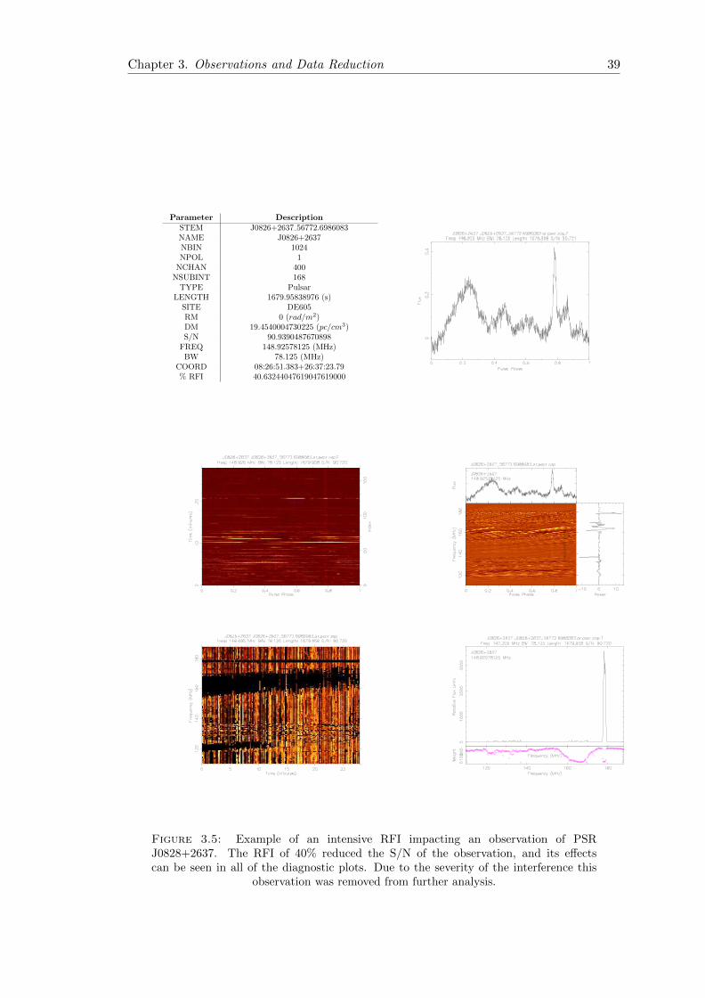
Chapter 3. Observations and Data Reduction 39
Parameter Description
STEM J0826+2637 56772.6986083NAME J0826+2637NBIN 1024NPOL 1
NCHAN 400NSUBINT 168
TYPE PulsarLENGTH 1679.95838976 (s)
SITE DE605RM 0 (rad/m2)DM 19.4540004730225 (pc/cm3)S/N 90.9390487670898
FREQ 148.92578125 (MHz)BW 78.125 (MHz)
COORD 08:26:51.383+26:37:23.79% RFI 40.63244047619047619000
Figure 3.5: Example of an intensive RFI impacting an observation of PSRJ0828+2637. The RFI of 40% reduced the S/N of the observation, and its effectscan be seen in all of the diagnostic plots. Due to the severity of the interference this
observation was removed from further analysis.
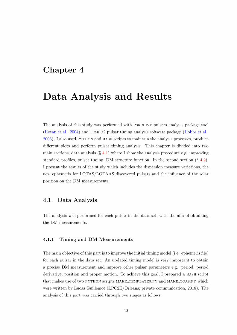
Chapter 4
Data Analysis and Results
The analysis of this study was performed with psrchive pulsars analysis package tool
(Hotan et al., 2004) and tempo2 pulsar timing analysis software package (Hobbs et al.,
2006). I also used python and bash scripts to maintain the analysis processes, produce
different plots and perform pulsar timing analysis. This chapter is divided into two
main sections, data analysis (§ 4.1) where I show the analysis procedure e.g. improving
standard profiles, pulsar timing, DM structure function. In the second section (§ 4.2),
I present the results of the study which includes the dispersion measure variations, the
new ephemeris for LOTAS/LOTAAS discovered pulsars and the influence of the solar
position on the DM measurements.
4.1 Data Analysis
The analysis was performed for each pulsar in the data set, with the aim of obtaining
the DM measurements.
4.1.1 Timing and DM Measurements
The main objective of this part is to improve the initial timing model (i.e. ephemeris file)
for each pulsar in the data set. An updated timing model is very important to obtain
a precise DM measurement and improve other pulsar parameters e.g. period, period
derivative, position and proper motion. To achieve this goal, I prepared a bash script
that makes use of two python scripts make templates.py and make toas.py which
were written by Lucas Guillemot (LPC2E/Orleans; private communication, 2018). The
analysis of this part was carried through two stages as follows:
40
Chapter 4. Data Analysis and Results 41
First Iteration
In this iteration, the RFI cleaned data was sub-divided to a number of sub-integrations
and sub-bands to check and improve the initial ephemeris of the data. Next, these data
were used to generate the first standard template and TOAs. Subsequently, tempo2
was used to obtain the timing residuals.
• The Standard Template Profile
This is the a typical profile for pulsar observations which is used to determine
their TOAs. In order to create a standard template from the reduced data, full-
intensity average profiles were created and averaged in time and frequency. Then,
the SNR was determined for each of these averaged profiles. Subsequently, a single
template was created, from all the observations of a specific pulsar, by adding the
top 10 profiles with the highest SNR. The summation of these profiles was done by
using psradd tool, where at this stage, the phase alignment between the added
profiles was applied by including the -P flag of the psradd tool. This stage was
illustrated in Figure 4.1, where panel (A) shows no alignment between the added
profile and panel (B) shows the profiles after the alignment was applied. Next, the
psrsmooth tool was also used to smooth the summed profiles which removed the
white noise from the profile data and increased the SNR.
• Time of Arrivals (TOAs)
In order to obtain DM measurements with better precision, the archives can be
divided into a number of frequency bands. The reason for this is that, the SNR
would be very low if we used each frequency channel individually. Similarly, for the
purpose of improving the period of each observation, the archives can be divided
into a number of sub-integrations. At this stage, all observations were split into
10 sub-integrations and 8 frequency bands across the total bandwidth, except the
recent observations of German stations (366 frequency channels), which were split
into 10 sub-integrations and 6 frequency bands. Also, a number of pulsars were
split into only 4 frequency channels due to their overall low SNR. The TOAs were
then obtained by using the cross-correlation techniques (see § 2.5.2) between the
observations and the generated template. In practise, this process was done by
using pat1 tool. The result of this process was a single file that contains TOAs of
all observations from a corresponding pulsar.
• Tempo2
The aim of this step is to obtain the timing residuals. At this stage, the generated
TOAs and the standard template were processed using tempo2 which involves
1http://psrchive.sourceforge.net/manuals/pat/
Chapter 4. Data Analysis and Results 42
(a)
(b)
Figure 4.1: The standard profile for J0139+5814 where panel (A) is the initial profiletemplate before applying the alignment which is created by identifying the highest 10SNR profiles and added to create a single template, then this template is smoothed.Panel (B) is the final profile template which is created by following the same procedure
of (A) but forcing the alignment between the profiles.
Chapter 4. Data Analysis and Results 43
fitting for a number of parameters. Depending on the pulsar, the fitting for spin
frequency (F0), its first derivative (F1) and DM can be sufficient to obtain the
timing solution, but for some pulsars, an additional fitting was required e.g. posi-
tion, proper motion etc, to obtain the desired solution. The final result was new
ephemeris that contains improved measurements for DM, period and other param-
eters. In order to produce a unified version of the ephemeris for all observations,
the command: “tempo2 -gr transform” was used to transform the version of the
ephemeris from tempo to tempo2.
Second Iteration
At this stage, all the observations were updated using the newly generated ephemeris
and then integrated in time and split into 8 sub-bands. The updated data were
then used to obtain a standard profile and final TOAs. Also, at this stage, a
number of TOAs were identified as clear outliers compared to the rest of TOAs.
Each of these outlying TOA was confirmed to be due to the high RFI or low SNR
of the observation and subsequently removed from further analysis. Removing
these outliers proved to be crucial in achieving better precision of the DM mea-
surements. The final result of this step was a file that contained the DM values
for each observation of a particular pulsar. This file was created by using the
command: “tempo2 -gr dm”
4.2 Results
4.2.1 New Timing Solutions for LOTAS/LOTAAS Sources
During the data reduction steps, I have obtained new timing models for three pulsars:
PSRs J0613+3731, J0815+4611 and J1740+27. Investigation of the diagnostic plots
for these sources has shown in the sub-integration stack that their periods were wrong
such that even within one observation one could see individual sub-integrations pulse
profile wrapping in phase. After noticing this, it was clear that this requires additional
corrections, by finding the right period within one observation, which was made by
using the psrchive tool pdmp2. Then, once the correct period was found, the raw data
were re-folded and the timing analysis was repeated. After correcting for the improper
period, the data went through my standard timing analysis in order to obtain the DM
measurements.
2http://psrchive.sourceforge.net/manuals/pdmp/
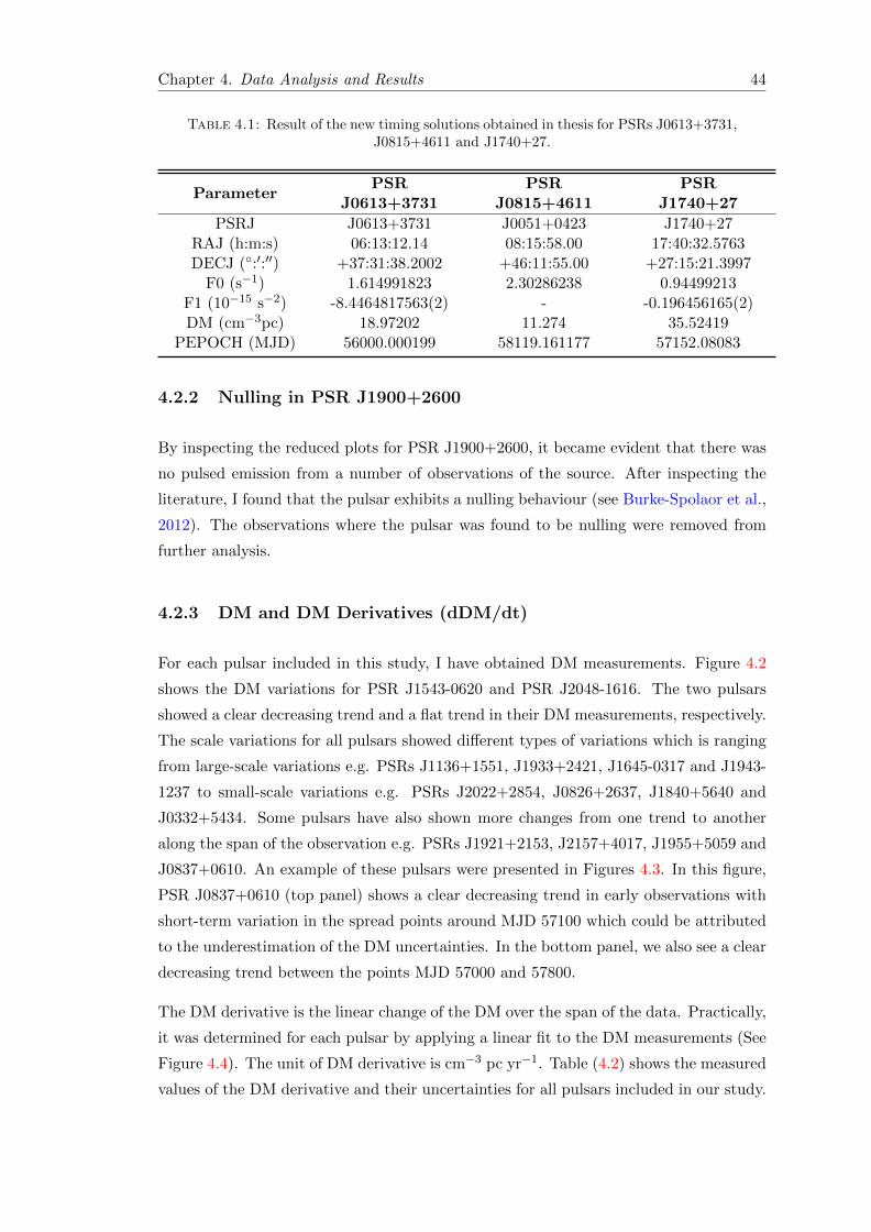
Chapter 4. Data Analysis and Results 44
Table 4.1: Result of the new timing solutions obtained in thesis for PSRs J0613+3731,J0815+4611 and J1740+27.
ParameterPSR
J0613+3731PSR
J0815+4611PSR
J1740+27
PSRJ J0613+3731 J0051+0423 J1740+27RAJ (h:m:s) 06:13:12.14 08:15:58.00 17:40:32.5763DECJ (:′:′′) +37:31:38.2002 +46:11:55.00 +27:15:21.3997
F0 (s−1) 1.614991823 2.30286238 0.94499213F1 (10−15 s−2) -8.4464817563(2) - -0.196456165(2)DM (cm−3pc) 18.97202 11.274 35.52419
PEPOCH (MJD) 56000.000199 58119.161177 57152.08083
4.2.2 Nulling in PSR J1900+2600
By inspecting the reduced plots for PSR J1900+2600, it became evident that there was
no pulsed emission from a number of observations of the source. After inspecting the
literature, I found that the pulsar exhibits a nulling behaviour (see Burke-Spolaor et al.,
2012). The observations where the pulsar was found to be nulling were removed from
further analysis.
4.2.3 DM and DM Derivatives (dDM/dt)
For each pulsar included in this study, I have obtained DM measurements. Figure 4.2
shows the DM variations for PSR J1543-0620 and PSR J2048-1616. The two pulsars
showed a clear decreasing trend and a flat trend in their DM measurements, respectively.
The scale variations for all pulsars showed different types of variations which is ranging
from large-scale variations e.g. PSRs J1136+1551, J1933+2421, J1645-0317 and J1943-
1237 to small-scale variations e.g. PSRs J2022+2854, J0826+2637, J1840+5640 and
J0332+5434. Some pulsars have also shown more changes from one trend to another
along the span of the observation e.g. PSRs J1921+2153, J2157+4017, J1955+5059 and
J0837+0610. An example of these pulsars were presented in Figures 4.3. In this figure,
PSR J0837+0610 (top panel) shows a clear decreasing trend in early observations with
short-term variation in the spread points around MJD 57100 which could be attributed
to the underestimation of the DM uncertainties. In the bottom panel, we also see a clear
decreasing trend between the points MJD 57000 and 57800.
The DM derivative is the linear change of the DM over the span of the data. Practically,
it was determined for each pulsar by applying a linear fit to the DM measurements (See
Figure 4.4). The unit of DM derivative is cm−3 pc yr−1. Table (4.2) shows the measured
values of the DM derivative and their uncertainties for all pulsars included in our study.
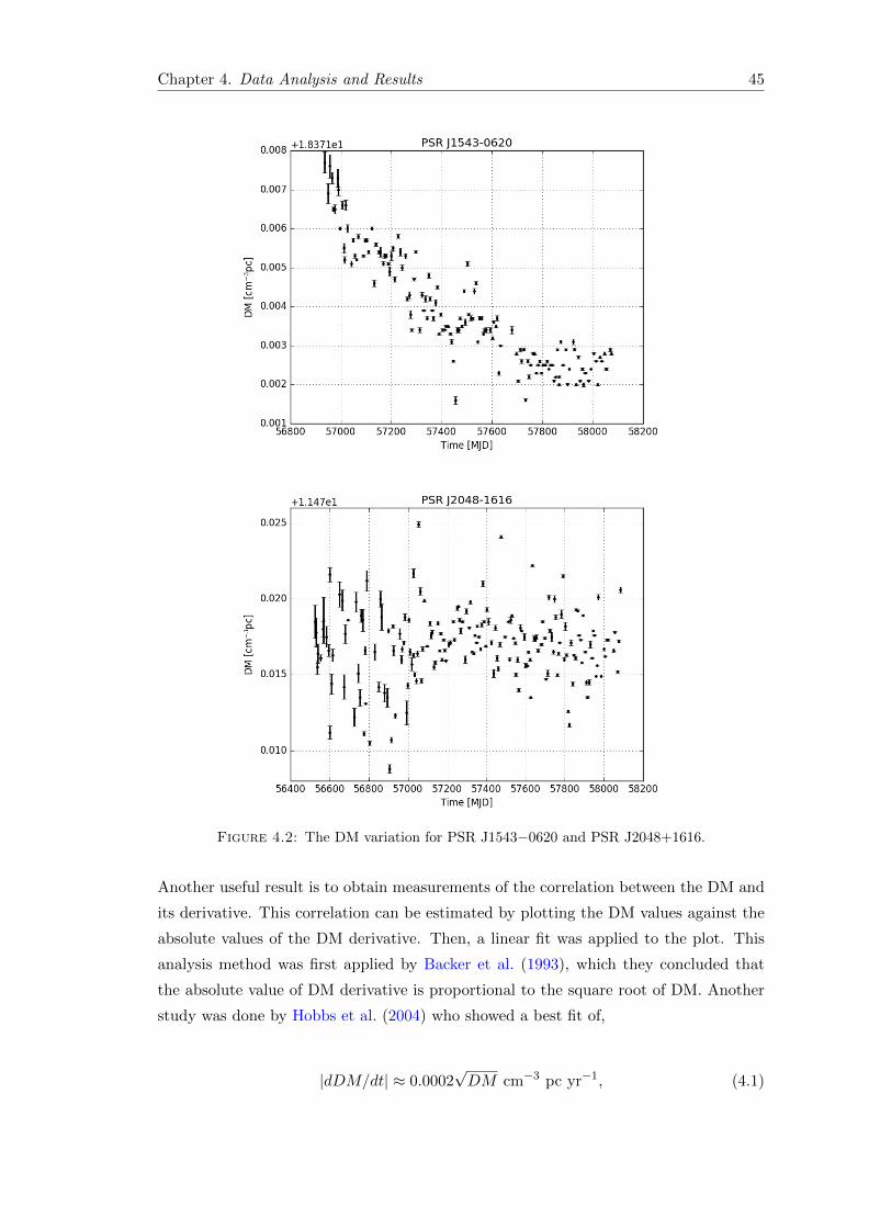
Chapter 4. Data Analysis and Results 45
Figure 4.2: The DM variation for PSR J1543−0620 and PSR J2048+1616.
Another useful result is to obtain measurements of the correlation between the DM and
its derivative. This correlation can be estimated by plotting the DM values against the
absolute values of the DM derivative. Then, a linear fit was applied to the plot. This
analysis method was first applied by Backer et al. (1993), which they concluded that
the absolute value of DM derivative is proportional to the square root of DM. Another
study was done by Hobbs et al. (2004) who showed a best fit of,
|dDM/dt| ≈ 0.0002√DM cm−3 pc yr−1, (4.1)
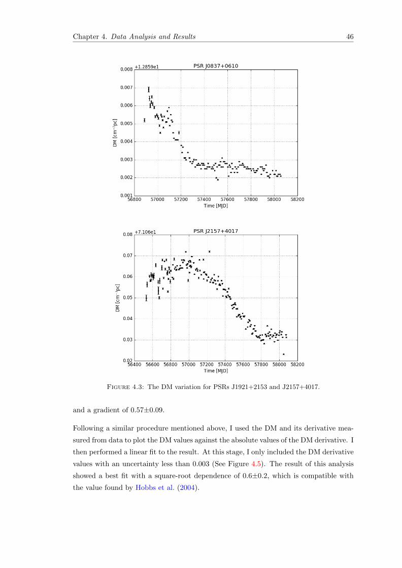
Chapter 4. Data Analysis and Results 46
Figure 4.3: The DM variation for PSRs J1921+2153 and J2157+4017.
and a gradient of 0.57±0.09.
Following a similar procedure mentioned above, I used the DM and its derivative mea-
sured from data to plot the DM values against the absolute values of the DM derivative. I
then performed a linear fit to the result. At this stage, I only included the DM derivative
values with an uncertainty less than 0.003 (See Figure 4.5). The result of this analysis
showed a best fit with a square-root dependence of 0.6±0.2, which is compatible with
the value found by Hobbs et al. (2004).
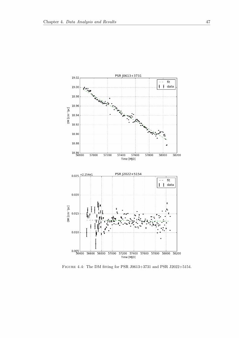
Chapter 4. Data Analysis and Results 47
Figure 4.4: The DM fitting for PSR J0613+3731 and PSR J2022+5154.
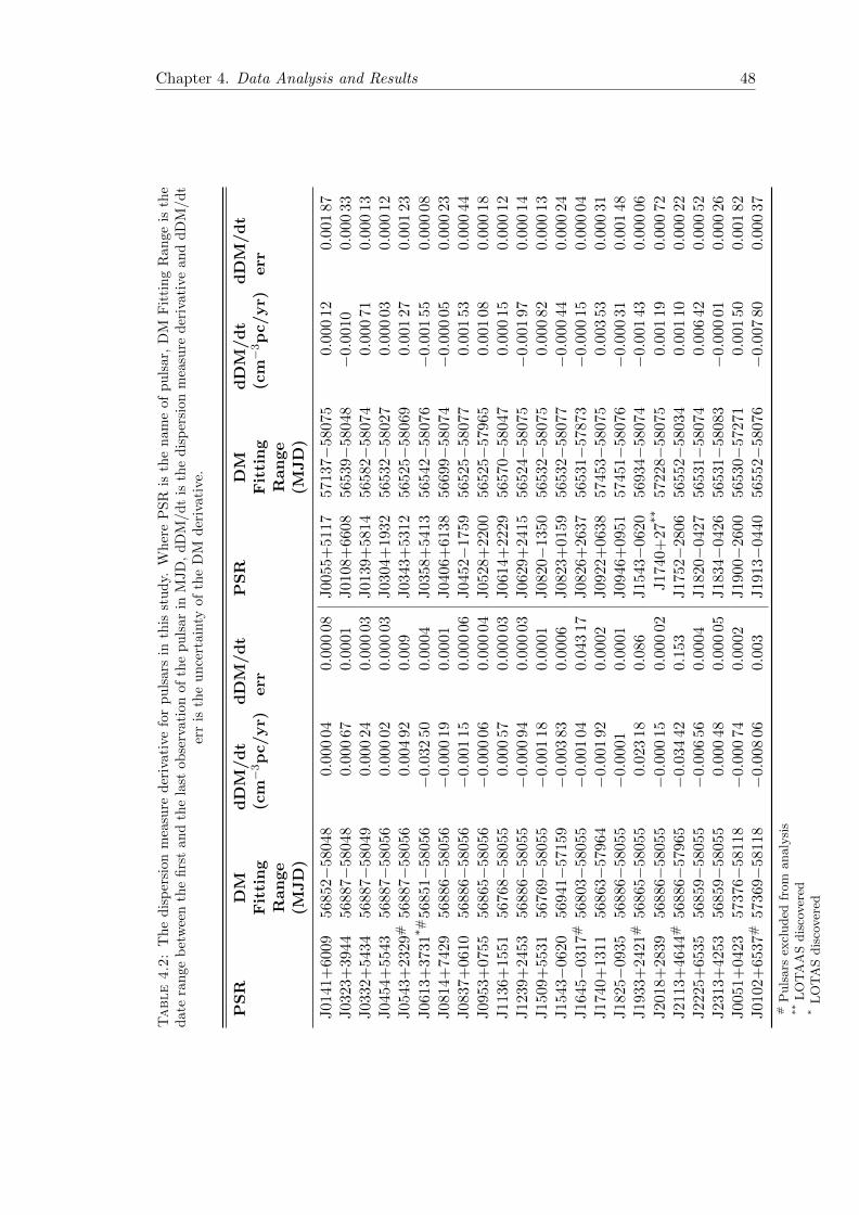
Chapter 4. Data Analysis and Results 48
Table4.2:
Th
ed
isp
ersi
onm
easu
red
eriv
ativ
efo
rp
uls
ars
inth
isst
ud
y.W
her
eP
SR
isth
en
am
eof
pu
lsar,
DM
Fit
tin
gR
an
ge
isth
ed
ate
ran
geb
etw
een
the
firs
tan
dth
ela
stob
serv
ati
on
of
the
pu
lsar
inM
JD
,d
DM
/d
tis
the
dis
per
sion
mea
sure
der
ivati
vean
dd
DM
/d
ter
ris
the
un
cert
ain
tyof
the
DM
der
ivati
ve.
PS
RD
MF
itti
ng
Ran
ge
(MJD
)
dD
M/d
t(c
m−
3p
c/yr)
dD
M/d
terr
PS
RD
MF
itti
ng
Ran
ge
(MJD
)
dD
M/d
t(c
m−
3p
c/yr)
dD
M/d
terr
J01
41+
6009
5685
2−58
048
0.00
004
0.0
0008
J00
55+
5117
5713
7−58
075
0.000
12
0.0
01
87
J03
23+
3944
5688
7−58
048
0.00
067
0.0
001
J01
08+
6608
5653
9−58
048
−0.
0010
0.0
00
33
J03
32+
5434
5688
7−58
049
0.00
024
0.0
0003
J01
39+
5814
5658
2−58
074
0.000
71
0.0
00
13
J04
54+
5543
5688
7−58
056
0.00
002
0.0
0003
J03
04+
1932
5653
2−58
027
0.000
03
0.0
00
12
J05
43+
2329
#56
887−
5805
60.
004
920.0
09J03
43+
5312
5652
5−58
069
0.001
27
0.0
01
23
J06
13+
3731
*#
5685
1−58
056
−0.0
3250
0.0
004
J03
58+
5413
5654
2−58
076
−0.
001
55
0.0
00
08
J08
14+
7429
5688
6−58
056
−0.
000
190.0
001
J04
06+
6138
5669
9−58
074
−0.
000
05
0.0
00
23
J08
37+
0610
5688
6−58
056
−0.
001
150.0
0006
J04
52−
1759
5652
5−58
077
0.001
53
0.0
00
44
J09
53+
0755
5686
5−58
056
−0.0
0006
0.0
0004
J05
28+
2200
5652
5−57
965
0.001
08
0.0
00
18
J11
36+
1551
5676
8−58
055
0.00
057
0.0
0003
J06
14+
2229
5657
0−58
047
0.000
15
0.0
00
12
J12
39+
2453
5688
6−58
055
−0.0
0094
0.0
0003
J06
29+
2415
5652
4−58
075
−0.
001
97
0.0
00
14
J15
09+
5531
5676
9−58
055
−0.
001
180.0
001
J08
20−
1350
5653
2−58
075
0.000
82
0.0
00
13
J15
43−
0620
5694
1−57
159
−0.0
0383
0.0
006
J08
23+
0159
5653
2−58
077
−0.
000
44
0.0
00
24
J16
45−
0317
#56
803−
5805
5−
0.0
0104
0.0
4317
J08
26+
2637
5653
1−57
873
−0.
000
15
0.0
00
04
J17
40+
1311
5686
3−57
964
−0.
001
920.0
002
J09
22+
0638
5745
3−58
075
0.003
53
0.0
00
31
J18
25−
0935
5688
6−58
055
−0.0
001
0.0
001
J09
46+
0951
5745
1−58
076
−0.
000
31
0.0
01
48
J19
33+
2421
#56
865−
5805
50.
023
180.0
86J15
43−
0620
5693
4−58
074
−0.
001
43
0.0
00
06
J20
18+
2839
5688
6−58
055
−0.
000
150.0
0002
J17
40+
27**
5722
8−
5807
50.
001
19
0.0
00
72
J21
13+
4644
#56
886−
5796
5−
0.03
442
0.1
53J17
52−
2806
5655
2−58
034
0.001
10
0.0
00
22
J22
25+
6535
5685
9−58
055
−0.0
0656
0.0
004
J18
20−
0427
5653
1−58
074
0.006
42
0.0
00
52
J23
13+
4253
5685
9−58
055
0.00
048
0.0
0005
J18
34−
0426
5653
1−58
083
−0.
000
01
0.0
00
26
J00
51+
0423
5737
6−58
118
−0.
000
740.0
002
J19
00−
2600
5653
0−57
271
0.001
50
0.0
01
82
J01
02+
6537
#57
369−
5811
8−
0.0
0806
0.0
03J19
13−
0440
5655
2−58
076
−0.
007
80
0.0
00
37
#Pulsars
excluded
from
analysis
**LOTAASdiscovered
*LOTASdiscovered
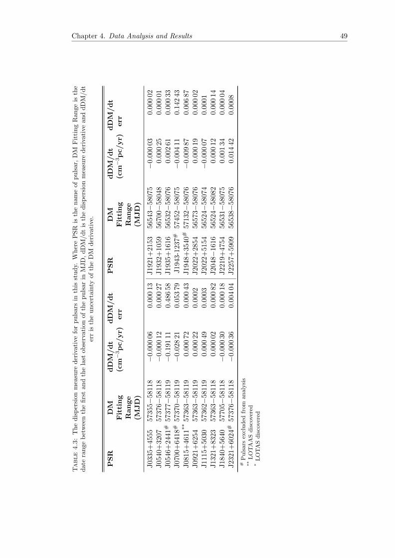
Chapter 4. Data Analysis and Results 49
Table4.3:
Th
ed
isp
ersi
onm
easu
red
eriv
ativ
efo
rp
uls
ars
inth
isst
ud
y.W
her
eP
SR
isth
en
am
eof
pu
lsar,
DM
Fit
tin
gR
an
ge
isth
ed
ate
ran
geb
etw
een
the
firs
tan
dth
ela
stob
serv
ati
on
of
the
pu
lsar
inM
JD
,d
DM
/d
tis
the
dis
per
sion
mea
sure
der
ivati
vean
dd
DM
/d
ter
ris
the
un
cert
ain
tyof
the
DM
der
ivati
ve.
PS
RD
MF
itti
ng
Ran
ge
(MJD
)
dD
M/d
t(c
m−
3p
c/yr)
dD
M/d
terr
PS
RD
MF
itti
ng
Ran
ge
(MJD
)
dD
M/d
t(c
m−
3p
c/yr)
dD
M/d
terr
J03
35+
4555
5735
5−58
118
−0.0
0006
0.0
0013
J19
21+
2153
5654
3−58
075
−0.
000
03
0.0
00
02
J05
40+
3207
5737
6−58
118
−0.
000
120.0
0027
J19
32+
1059
5670
0−58
048
0.000
25
0.0
00
01
J05
46+
2441
#57
377−
5811
9−
0.1
9111
0.4
8658
J19
35+
1616
5653
2−58
076
0.002
61
0.0
00
33
J07
00+
6418
#57
370−
5811
9−
0.0
2821
0.0
5379
J19
43-1
237
#57
452−
5807
5−
0.004
11
0.1
42
43
J08
15+
4611
**
5736
3−58
119
0.00
072
0.0
0043
J19
48+
3540
#57
132−
5807
6−
0.009
87
0.0
06
87
J09
21+
6254
5736
3−58
119
0.00
022
0.0
002
J20
22+
2854
5657
3−58
076
0.000
19
0.0
00
02
J11
15+
5030
5736
2−58
119
0.00
049
0.0
003
J20
22+
5154
5652
4−58
074
−0.
000
07
0.0
001
J13
21+
8323
5736
3−58
118
0.00
002
0.0
0082
J20
48−
1616
5652
4−58
082
0.000
12
0.0
00
14
J18
40+
5640
5770
5−58
118
−0.0
0030
0.0
0018
J22
19+
4754
5653
1−58
075
0.001
34
0.0
00
04
J23
21+
6024
#57
376−
5811
8−
0.0
0036
0.0
0404
J22
57+
5909
5653
8−58
076
0.014
42
0.0
008
#Pulsars
excluded
from
analysis
**LOTAASdiscovered
*LOTASdiscovered
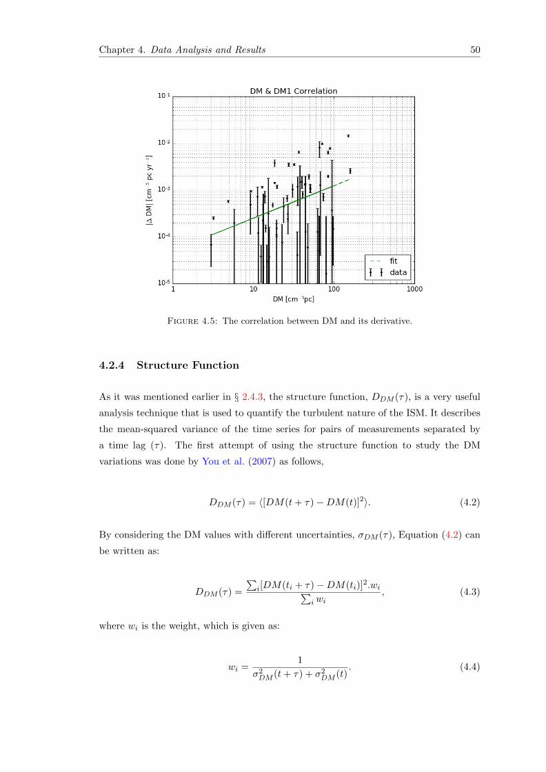
Chapter 4. Data Analysis and Results 50
Figure 4.5: The correlation between DM and its derivative.
4.2.4 Structure Function
As it was mentioned earlier in § 2.4.3, the structure function, DDM (τ), is a very useful
analysis technique that is used to quantify the turbulent nature of the ISM. It describes
the mean-squared variance of the time series for pairs of measurements separated by
a time lag (τ). The first attempt of using the structure function to study the DM
variations was done by You et al. (2007) as follows,
DDM (τ) = 〈[DM(t+ τ)−DM(t)]2〉. (4.2)
By considering the DM values with different uncertainties, σDM (τ), Equation (4.2) can
be written as:
DDM (τ) =
∑i[DM(ti + τ)−DM(ti)]
2.wi∑iwi
, (4.3)
where wi is the weight, which is given as:
wi =1
σ2DM (t+ τ) + σ2
DM (t). (4.4)
Chapter 4. Data Analysis and Results 51
For a particular case of the Kolmogorov power-law spectrum, the structure function is
represented by,
DDM (τ) = (τ/τd)5/3. (4.5)
Where τ is the time lag and τd is the diffractive time scale.
Figure 4.6 shows the result of structure function for PSR J1543−0620, which shows
a structure consistent with the Kolmogorov spectrum, starting from the time-lag be-
tween 100 and 1000 days. This also indicates the inhomogeneous turbulent structure of
the ISM. PSR J0953+0755 shows an inconsistent result compared to the Kolmogorov
structure, which could also indicate the presence of the homogeneous structure of the
ISM.
After I have obtained the time-dependent DM measurements with their uncertainties,
I tried to obtain the structure function directly from these measurements. This can be
done by applying an evenly spaced time lag (τ) over the span of the observations and
applying Equation (4.2) to obtain the structure function. During the data reductions
and analysis, some observations were removed due to many reasons (e.g. RFI, insufficient
sub-integrations and frequency channels). As a result of this removal, there were missing
values and therefore, it was not possible to generate measurements with an evenly spaced
time lag over the span of the observations. In order to solve for this problem, I performed
a Gaussian Process (GP) Regression analysis by trying two tools: the python library
George3 and GPy4 (using the radial basis function kernel i.e. RBF kernel), which
are both used to obtain a likelihood of the missing part of the data. The predicted
measurements are highly dependent on the measured DM and its uncertainty across the
span of the data. Using these probabilities to obtain the best estimated values could
enable us to create evenly spaced time intervals and associated DM measurements to
determine the structure function. However, this approach was unsuccessful, due to the
large scattering of the DM measurements as reflected in the uncertainties of the GP
output (See Figure 4.7).
4.2.5 DM Variations and the Solar Angle
In pulsar timing, the solar wind can have a significant influence on the measurements of
the DM itself. In order to check for this effect, I first assumed an angular distance from
the Sun <= 20 for observations which could be affected by the solar wind. Next, for
3https://george.readthedocs.io/en/latest/4http://sheffieldml.github.io/GPy/

Chapter 4. Data Analysis and Results 52
Figure 4.6: The DM structure function for PSR J1543−0620 and PSR J0953+0755.
each observation, I calculated the solar angle, then plotted it with the corresponding DM
values. Inspection of those plots revealed that there was no significant influence of the
solar wind on my DM measurements. Figure 4.8 shows an example of the observations
of PSR J0614+2229.
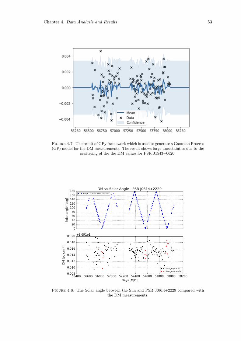
Chapter 4. Data Analysis and Results 53
Figure 4.7: The result of GPy framework which is used to generate a Gaussian Process(GP) model for the DM measurements. The result shows large uncertainties due to the
scattering of the the DM values for PSR J1543−0620.
Figure 4.8: The Solar angle between the Sun and PSR J0614+2229 compared withthe DM measurements.
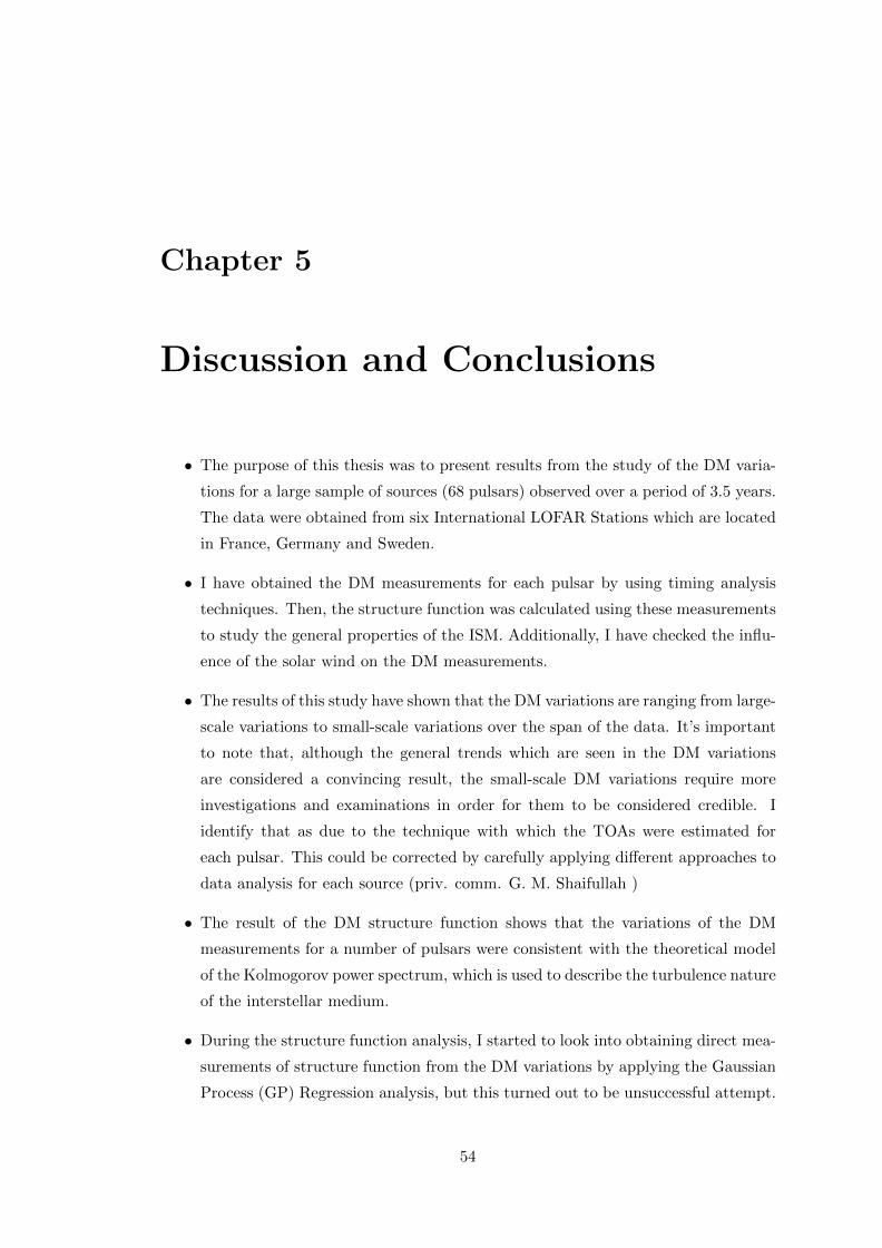
Chapter 5
Discussion and Conclusions
• The purpose of this thesis was to present results from the study of the DM varia-
tions for a large sample of sources (68 pulsars) observed over a period of 3.5 years.
The data were obtained from six International LOFAR Stations which are located
in France, Germany and Sweden.
• I have obtained the DM measurements for each pulsar by using timing analysis
techniques. Then, the structure function was calculated using these measurements
to study the general properties of the ISM. Additionally, I have checked the influ-
ence of the solar wind on the DM measurements.
• The results of this study have shown that the DM variations are ranging from large-
scale variations to small-scale variations over the span of the data. It’s important
to note that, although the general trends which are seen in the DM variations
are considered a convincing result, the small-scale DM variations require more
investigations and examinations in order for them to be considered credible. I
identify that as due to the technique with which the TOAs were estimated for
each pulsar. This could be corrected by carefully applying different approaches to
data analysis for each source (priv. comm. G. M. Shaifullah )
• The result of the DM structure function shows that the variations of the DM
measurements for a number of pulsars were consistent with the theoretical model
of the Kolmogorov power spectrum, which is used to describe the turbulence nature
of the interstellar medium.
• During the structure function analysis, I started to look into obtaining direct mea-
surements of structure function from the DM variations by applying the Gaussian
Process (GP) Regression analysis, but this turned out to be unsuccessful attempt.
54
Bibliography 55
This is most likely due to the aforementioned TOAs error measurements and after
appropriate improvements deserve its own study.
• I have also calculated the correlations between the DM and their derivatives. The
obtained result of this correlation was shown a square-root dependence of 0.6±0.2
which is comparable with the previously published results (e.g. Hobbs et al., 2004).
• One of the major results of my study was obtaining new timing solutions for three
pulsars: PSRs J0613+3731, J0815+4611 and J1740+27. These improved solu-
tions can be used in ongoing observations with e.g. LOFAR Core or International
LOFAR Stations.
• I have prepared an automated data reduction pipeline which was invaluable given
the large amount of observations to process. For some pulsars, data analysis result
have shown that to have that an individual approach is required in order to process
them correctly (e.g. the polarization calibration techniques presented in Tiburzi
et al. (submitted) and Donner et al. (in prep)). These approaches are out of the
scope of this study.
• Typical publications of DM variations use data over 5−6 years as a minimum time
span. There is already a larger sample of pulsar observations, including millisecond
pulsars (MSPs), taken over longer period of time (i.e. 5 years) compared to what
was used during this study. For future studies these observations could be used
to obtain a higher quality result. Additionally, there is a wealth of information
that can be learned by trying the low-frequency observations from LOFAR with
the higher frequency observations from a telescope like the Westerbork Synthesis
Radio Telescope (WSRT), which observed sources in P band (i.e. 250 to 500 MHz)
and L band (i.e. 0.5 to 1.5 GHz) (See Karuppusamy et al. 2008). This ultimately
could enable us to improve DM measurements as well as timing analysis of selected
sources observed by both telescopes.
Bibliography
Armstrong, J., Rickett, B., and Spangler, S. (1995). Electron density power spectrum
in the local interstellar medium. The Astrophysical Journal, 443:209–221.
Baade, W. and Zwicky, F. (1934). Remarks on super-novae and cosmic rays. Physical
Review, 46(1):76.
Backer, D., Hama, S., Van Hook, S., and Foster, R. (1993). Temporal variations of
pulsar dispersion measures. The Astrophysical Journal, 404:636–642.
Backer, D. C., Kulkarni, S. R., Heiles, C., Davis, M., and Goss, W. (1982). A millisecond
pulsar. Nature, 300(5893):615–618.
Bailes, M., Barr, E., Bhat, N., Brink, J., Buchner, S., Burgay, M., Camilo, F., Champion,
D., Hessels, J., Janssen, G., et al. (2018). Meertime-the meerkat key science program
on pulsar timing. arXiv preprint arXiv:1803.07424.
Burgay, M., D’amico, N., Possenti, A., Manchester, R., Lyne, A., Joshi, B., McLaughlin,
M., Kramer, M., Sarkissian, J., Camilo, F., et al. (2003). An increased estimate of the
merger rate of double neutron stars from observations of a highly relativistic system.
Nature, 426(6966):531–533.
Burke-Spolaor, S., Johnston, S., Bailes, M., Bates, S., Bhat, N., Burgay, M., Champion,
D., D’Amico, N., Keith, M., Kramer, M., et al. (2012). The high time resolution
universe pulsar survey–v. single-pulse energetics and modulation properties of 315
pulsars. Monthly Notices of the Royal Astronomical Society, 423(2):1351–1367.
Camilo, F., Ransom, S. M., Halpern, J. P., Reynolds, J., Helfand, D. J., Zimmerman, N.,
and Sarkissian, J. (2006). Transient pulsed radio emission from a magnetar. Nature,
442(7105):892–895.
Coenen, T., Van Leeuwen, J., Hessels, J. W., Stappers, B. W., Kondratiev, V. I., Alexov,
A., Breton, R., Bilous, A., Cooper, S., Falcke, H., et al. (2014). The lofar pilot surveys
for pulsars and fast radio transients. Astronomy & astrophysics, 570:A60.
56
Bibliography 57
Cordes, J. M., Shannon, R. M., and Stinebring, D. R. (2016). Frequency-dependent
dispersion measures and implications for pulsar timing. The Astrophysical Journal,
817(1):16.
Dabrowski, B. P., Krankowski, A., Baszkiewicz, L., and Rothkaehl, H. (2016). Prospects
for solar and space weather research with polish part of the lofar telescope. Acta
Geophysica, 64(3):825–840.
Donner, J. (2017). Lofar studies of the ionised interstellar medium at the smallest scales.
Duncan, R. C. and Thompson, C. (1992). Formation of very strongly magnetized neutron
stars-implications for gamma-ray bursts. The Astrophysical Journal, 392:L9–L13.
Edwards, R. T., Hobbs, G., and Manchester, R. (2006). tempo2, a new pulsar timing
package–ii. the timing model and precision estimates. Monthly Notices of the Royal
Astronomical Society, 372(4):1549–1574.
Field, G., Goldsmith, D., and Habing, H. (1969). Cosmic-ray heating of the interstellar
gas. The Astrophysical Journal, 155:L149.
Goldreich, P. and Julian, W. H. (1969). Pulsar electrodynamics. The Astrophysical
Journal, 157:869.
Gunn, J. and Ostriker, J. (1970). On the nature of pulsars. iii. analysis of observations.
The Astrophysical Journal, 160:979.
Harding, A. K. (2013). The neutron star zoo. Frontiers of Physics, 8(6):679–692.
Hessels, J. W., Ransom, S. M., Stairs, I. H., Freire, P. C., Kaspi, V. M., and Camilo, F.
(2006). A radio pulsar spinning at 716 hz. Science, 311(5769):1901–1904.
Hewish, A., Bell, S. J., Pilkington, J., Scott, P. F., and Collins, R. A. (1968). Observation
of a rapidly pulsating radio source. Nature, 217(5130):709–713.
Hobbs, G. (2009). Pulsar timing array projects. Proceedings of the International Astro-
nomical Union, 5(S261):228–233.
Hobbs, G., Archibald, A., Arzoumanian, Z., Backer, D., Bailes, M., Bhat, N., Burgay,
M., Burke-Spolaor, S., Champion, D., Cognard, I., et al. (2010). The international
pulsar timing array project: using pulsars as a gravitational wave detector. Classical
and Quantum Gravity, 27(8):084013.
Hobbs, G., Edwards, R., and Manchester, R. (2006). Tempo2, a new pulsar-
timing package–i. an overview. Monthly Notices of the Royal Astronomical Society,
369(2):655–672.
Bibliography 58
Hobbs, G., Lyne, A., Kramer, M., Martin, C., and Jordan, C. (2004). Long-term
timing observations of 374 pulsars. Monthly Notices of the Royal Astronomical Society,
353(4):1311–1344.
Hotan, A. W., Van Straten, W., and Manchester, R. (2004). Psrchive and psrfits:
an open approach to radio pulsar data storage and analysis. Publications of the
Astronomical Society of Australia, 21(3):302–309.
Karuppusamy, R., Stappers, B., and Van Straten, W. (2008). Puma-ii: a wide band
pulsar machine for the westerbork synthesis radio telescope. Publications of the As-
tronomical Society of the Pacific, 120(864):191.
Keane, E. F. (2010). The Transient Radio Sky. PhD thesis, University of Manchester.
Lattimer, J. and Prakash, M. (2001). Neutron star structure and the equation of state.
The Astrophysical Journal, 550(1):426.
Lazarus, P., Karuppusamy, R., Graikou, E., Caballero, R., Champion, D., Lee, K.,
Verbiest, J., and Kramer, M. (2016). Prospects for high-precision pulsar timing with
the new effelsberg psrix backend. Monthly Notices of the Royal Astronomical Society,
458(1):868–880.
Lewin, W. and Van der Klis, M. (2006). Compact stellar X-ray sources, volume 39.
Cambridge University Press.
Lorimer, D. R. (2001). Binary and millisecond pulsars at the new millennium. Living
Reviews in Relativity, 4(1):5.
Lorimer, D. R. and Kramer, M. (2005). Handbook of pulsar astronomy. Cambridge
University Press.
Lyne, A. and Graham-Smith, F. (2012). Pulsar astronomy. Number 48. Cambridge
University Press.
Lyne, A. and Lorimer, D. (1994). High birth velocities of radio pulsars. Nature,
369(6476):127–129.
Manchester, R. (2017). Pulsar timing and its applications. In Journal of Physics:
Conference Series, volume 932, page 012002. IOP Publishing.
Manchester, R. N., Hobbs, G. B., Teoh, A., and Hobbs, M. (2005). The Australia
Telescope National Facility Pulsar Catalogue. aj, 129:1993–2006.
McKay-Bukowski, D., Vierinen, J., Virtanen, I. I., Fallows, R., Postila, M., Ulich,
T., Wucknitz, O., Brentjens, M., Ebbendorf, N., Enell, C.-F., et al. (2015). Kaira:
Bibliography 59
The kilpisjarvi atmospheric imaging receiver array—system overview and first results.
IEEE Transactions on Geoscience and Remote Sensing, 53(3):1440–1451.
McKee, C. F. and Ostriker, J. P. (1977). A theory of the interstellar medium-three
components regulated by supernova explosions in an inhomogeneous substrate. The
Astrophysical Journal, 218:148–169.
McLaughlin, M. A., Lyne, A., Lorimer, D., Kramer, M., Faulkner, A., Manchester, R.,
Cordes, J., Camilo, F., Possenti, A., Stairs, I., et al. (2006). Transient radio bursts
from rotating neutron stars. Nature, 439(7078):817–820.
Olausen, S. and Kaspi, V. (2014). The mcgill magnetar catalog. The Astrophysical
Journal Supplement Series, 212(1):6.
Oppenheimer, J. R. and Volkoff, G. M. (1939). On massive neutron cores. Physical
Review, 55(4):374.
Pacini, F. (1967). Energy emission from a neutron star. Nature, 216(5115):567–568.
Pitkin, M. (2018). psrqpy: a python interface for querying the ATNF pulsar catalogue.
Journal of Open Source Software, 3(22):538.
Rickett, B. J. (1990). Radio propagation through the turbulent interstellar plasma.
Annual review of astronomy and astrophysics, 28(1):561–605.
Ruderman, M. A. and Sutherland, P. G. (1975). Theory of pulsars-polar caps, sparks,
and coherent microwave radiation. The Astrophysical Journal, 196:51–72.
Stappers, B., Hessels, J., Alexov, A., Anderson, K., Coenen, T., Hassall, T., Karaster-
giou, A., Kondratiev, V., Kramer, M., Van Leeuwen, J., et al. (2011). Observing
pulsars and fast transients with lofar. Astronomy & astrophysics, 530:A80.
Sturrock, P. (1971). A model of pulsars. The Astrophysical Journal, 164:529.
Taylor, J. H. (1992). Pulsar timing and relativistic gravity. Phil. Trans. R. Soc. Lond.
A, 341(1660):117–134.
Taylor, J. H. and Weisberg, J. M. (1982). A new test of general relativity-gravitational
radiation and the binary pulsar psr 1913+ 16. The Astrophysical Journal, 253:908–920.
Tyul’bashev, S. A., Tyul’bashev, V. S., and Malofeev, V. M. (2018). Detection of 25
new rotating radio transients at 111 mhz. arXiv preprint arXiv:1807.07565.
van Haarlem, M. a., Wise, M., Gunst, A., Heald, G., McKean, J., Hessels, J., De Bruyn,
A., Nijboer, R., Swinbank, J., Fallows, R., et al. (2013). Lofar: The low-frequency
array. Astronomy & Astrophysics, 556:A2.
Bibliography 60
Verbiest, J., Lentati, L., Hobbs, G., van Haasteren, R., Demorest, P. B., Janssen, G.,
Wang, J.-B., Desvignes, G., Caballero, R., Keith, M., et al. (2016). The international
pulsar timing array: first data release. Monthly Notices of the Royal Astronomical
Society, 458(2):1267–1288.
Wielebinski, R. (2002). The Characteristics of (Normal) Pulsars. In Becker, W., Lesch,
H., and Trumper, J., editors, Neutron Stars, Pulsars, and Supernova Remnants, page
167.
Williamson, I. P. (1972). Pulse broadening due to multiple scattering in the interstellar
medium. Monthly Notices of the Royal Astronomical Society, 157(1):55–71.
You, X.-P., Hobbs, G., Coles, W. A., Manchester, R. N., Edwards, R., Bailes, M.,
Sarkissian, J., Verbiest, J. P., Van Straten, W., Hotan, A., et al. (2007). Dispersion
measure variations and their effect on precision pulsar timing. Monthly Notices of the
Royal Astronomical Society, 378(2):493–506.
Zarka, P., Tagger, M., Denis, L., Girard, J., Konovalenko, A., Atemkeng, M., Arnaud,
M., Azarian, S., Barsuglia, M., Bonafede, A., et al. (2015). Nenufar: Instrument
description and science case. In Antenna Theory and Techniques (ICATT), 2015
International Conference on, pages 1–6. IEEE.