Dispersion in Optical Fibers

By Gildas Chauvel – Anritsu Corporation

TABLE OF CONTENTS

Introduction

Chromatic Dispersion (CD): Definition and Origin; Limit and Compensation; and Measurement Methods

Polarization Mode Dispersion (PMD): Definition and Origin; Statistical Nature; Limit and Compensation; and Measurement Methods

Conclusion

Introduction Telecommunications service providers have to face continuously growing bandwidth demands in all networks areas, from long-haul to access. Because installing new communication links would require huge investments, telecommunications carriers prefer to increase the capacity of their existing fiber links by using dense wavelength-division multiplexing (DWDM) systems and/or higher bit rates systems. However, most of the installed optical fibers are old and exhibit physical characteristics that may limit their ability to transmit high-speed signals. The broadening of light pulses, called dispersion, is a critical factor limiting the quality of signal transmission over optical links. Dispersion is a consequence of the physical properties of the transmission medium. Single-mode fibers, used in high-speed optical networks, are subject to Chromatic Dispersion (CD) that causes pulse broadening depending on wavelength, and to Polarization Mode Dispersion (PMD) that causes pulse broadening depending on polarization. Excessive spreading will cause bits to “overflow” their intended time slots and overlap adjacent bits. The receiver may then have difficulty discerning and properly interpreting adjacent bits, increasing the Bit Error Rate. To preserve the transmission quality, the maximum amount of time dispersion must be limited to a small proportion of the signal bit rate, typically 10% of the bit time. With optical networks moving from 2.5 Gbps to 10 Gbps and onto 40 Gbps, the acceptable tolerance of dispersion is drastically reduced. For instance, the amount of acceptable chromatic dispersion decreases by a factor of 16 when moving from 2.5 to 10 Gbps, and by an additional factor of 16 moving from 10 to 40 Gbps. These tight tolerances of high-speed networks mean that every possible source of pulse spreading should be addressed. Operating companies need to measure the dispersion of their networks to assess the possibility of upgrading them to higher transmission speeds, or to evaluate the need for compensation. This paper presents the causes and effects of dispersion and describes the different ways to measure it.

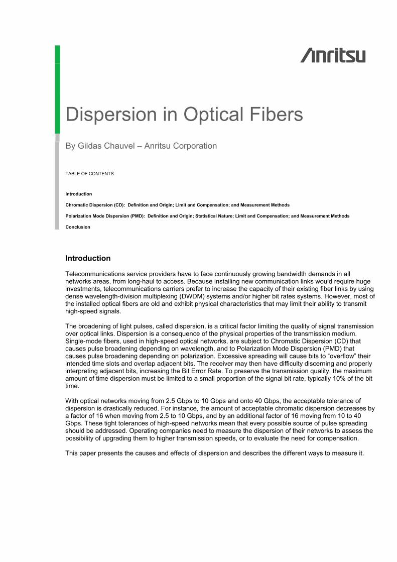
Chromatic Dispersion (CD) CD Definition and Origin Light within a medium travels at a slower speed than in vacuum. The speed at which light travels is determined by the medium’s refractive index. In an ideal situation, the refractive index would not depend on the wavelength of the light. Since this is not the case, different wavelengths travel at different speeds within an optical fiber.

Figure 1: CD in single-mode fiber

Laser sources are spectrally thin, but not monochromatic. This means that the input pulse contains several wavelength components, traveling at different speeds, causing the pulse to spread. The detrimental effects of chromatic dispersion result in the slower wavelengths of one pulse intermixing with the faster wavelengths of an adjacent pulse, causing intersymbol interference. The Chromatic Dispersion of a fiber is expressed in ps/(nm*km), representing the differential delay, or time spreading (in ps), for a source with a spectral width of 1 nm traveling on 1 km of the fiber. It depends on the fiber type, and it limits the bit rate or the transmission distance for a good quality of service. CD of current network spans As a consequence of its optical characteristics, the Chromatic Dispersion of a fiber can be changed by acting on the physical properties of the material. To reduce fiber dispersion, new types of fiber were invented, including dispersion-shifted fibers (ITU G.653) and non-zero dispersion-shifted fiber (ITU G.655). The most commonly deployed fiber in networks (ITU G.652), called “dispersion-unshifted” singlemode fiber, has a small chromatic dispersion in the optical window around 1310 nm, but exhibits a higher CD in the 1550 nm region. This dispersion limits the possible transmission length without compensation on OC-768/STM-256 DWDM networks. ITU G.653 is a dispersion-shifted fiber (DSF), designed to minimize chromatic dispersion in the 1550 nm window with zero dispersion between 1525 nm and 1575 nm. But this type of fiber has several drawbacks, such as higher polarization mode dispersion than ITU G.652, and a high Four Wave Mixing risk, rendering DWDM practically impossible. For these reasons, another singlemode fiber was developed: the Non-Zero Dispersion-Shifted Fiber (NZDSF). NZDSF fibers have now replaced DSF fibers, which are not used anymore. The ITU G.655 Non-Zero Dispersion-Shifted Fibers were developed to eliminate non-linear effects experienced on DSF fibers. They were developed especially for DWDM applications in the 1550 nm window. They have a cut-off wavelength around 1310 nm, limiting their operation around this wavelength.

Poly-chromatic incident light

λ1 λ2

Single-Mode Fiber

Refractive index: n(λ)

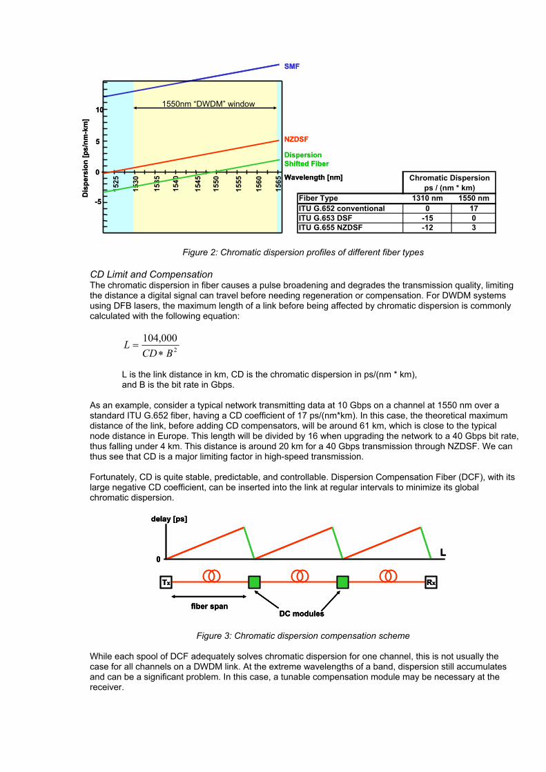
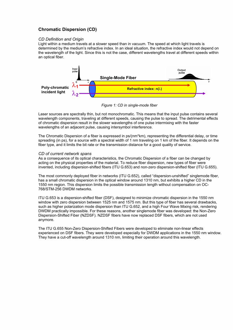
Figure 2: Chromatic dispersion profiles of different fiber types CD Limit and Compensation The chromatic dispersion in fiber causes a pulse broadening and degrades the transmission quality, limiting the distance a digital signal can travel before needing regeneration or compensation. For DWDM systems using DFB lasers, the maximum length of a link before being affected by chromatic dispersion is commonly calculated with the following equation:

2

000,104BCD

L∗

=

L is the link distance in km, CD is the chromatic dispersion in ps/(nm * km), and B is the bit rate in Gbps.

As an example, consider a typical network transmitting data at 10 Gbps on a channel at 1550 nm over a standard ITU G.652 fiber, having a CD coefficient of 17 ps/(nm*km). In this case, the theoretical maximum distance of the link, before adding CD compensators, will be around 61 km, which is close to the typical node distance in Europe. This length will be divided by 16 when upgrading the network to a 40 Gbps bit rate, thus falling under 4 km. This distance is around 20 km for a 40 Gbps transmission through NZDSF. We can thus see that CD is a major limiting factor in high-speed transmission. Fortunately, CD is quite stable, predictable, and controllable. Dispersion Compensation Fiber (DCF), with its large negative CD coefficient, can be inserted into the link at regular intervals to minimize its global chromatic dispersion.

Tx Rx

DC modulesfiber span

delay [ps]

0L

Tx Rx

DC modulesfiber span

Tx Rx

DC modulesfiber span

delay [ps]

0L

delay [ps]

0L

Figure 3: Chromatic dispersion compensation scheme While each spool of DCF adequately solves chromatic dispersion for one channel, this is not usually the case for all channels on a DWDM link. At the extreme wavelengths of a band, dispersion still accumulates and can be a significant problem. In this case, a tunable compensation module may be necessary at the receiver.

Dis

pers

ion

[ps/

nm-k

m]

1525

1530

1535

1540

1545

1550

1555

1560

SMF

NZDSF

Dispersion Shifted Fiber

5

0

-5

Wavelength [nm]

101550nm “DWDM” window

1565

Dis

pers

ion

[ps/

nm-k

m]

1525

1530

1535

1540

1545

1550

1555

1560

SMF

NZDSF

Dispersion Shifted Fiber

5

0

-5

Wavelength [nm]

101550nm “DWDM” window

1565

Fiber Type 1310 nm 1550 nmITU G.652 conventional 0 17ITU G.653 DSF -15 0ITU G.655 NZDSF -12 3

Chromatic Dispersionps / (nm * km)

delay [ps]

0

λ1λ2λ3

delay [ps]

0

λ1λ2λ3

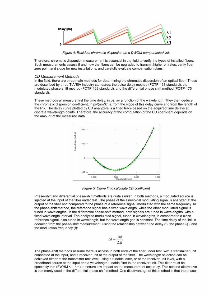
Figure 4: Residual chromatic dispersion on a DWDM-compensated link Therefore, chromatic dispersion measurement is essential in the field to verify the types of installed fibers. Such measurements assess if and how the fibers can be upgraded to transmit higher bit rates, verify fiber zero point and slope for new installations, and carefully evaluate compensation plans. CD Measurement Methods In the field, there are three main methods for determining the chromatic dispersion of an optical fiber. These are described by three TIA/EIA industry standards: the pulse-delay method (FOTP-168 standard), the modulated phase-shift method (FOTP-169 standard), and the differential phase shift method (FOTP-175 standard). These methods all measure first the time delay, in ps, as a function of the wavelength. They then deduce the chromatic dispersion coefficient, in ps/(nm*km), from the slope of this delay curve and from the length of the link. The delay curve plotted by CD analyzers is a fitted trace based on the acquired time delays at discrete wavelength points. Therefore, the accuracy of the computation of the CD coefficient depends on the amount of the measured data.

Figure 5: Curve fit to calculate CD coefficient Phase-shift and differential phase-shift methods are quite similar. In both methods, a modulated source is injected at the input of the fiber under test. The phase of the sinusoidal modulating signal is analyzed at the output of the fiber and compared to the phase of a reference signal, modulated with the same frequency. In the phase-shift method, the reference signal has a fixed wavelength, while the other modulated signal is tuned in wavelengths. In the differential phase-shift method, both signals are tuned in wavelengths, with a fixed wavelength interval. The analyzed modulated signal, tuned in wavelengths, is compared to a close reference signal, also tuned in wavelength, but the wavelength gap is constant. The time delay of the link is deduced from the phase-shift measurement, using the relationship between the delay (t), the phase (φ), and the modulation frequency (f):

ft

πφ

2∆

=∆

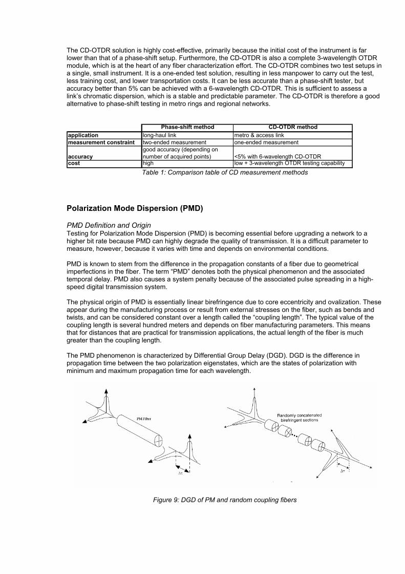
The phase-shift methods assume there is access to both ends of the fiber under test, with a transmitter unit connected at the input, and a receiver unit at the output of the fiber. The wavelength selection can be achieved either at the transmitter unit level, using a tunable laser, or at the receiver unit level, with a broadband source at the input and a wavelength tunable filter in the receiver unit. This filter must be spectrally thin (FWHM < 1 nm) to ensure low impact on the measurement accuracy. This second alternative is commonly used in the differential phase-shift method. One disadvantage of this method is that the phase-

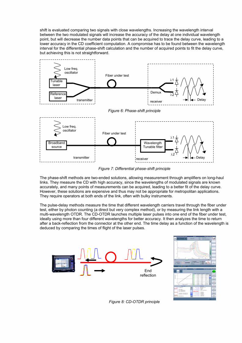
shift is evaluated comparing two signals with close wavelengths. Increasing the wavelength interval between the two modulated signals will increase the accuracy of the delay at one individual wavelength point, but will decrease the number data points that can be acquired to trace the delay curve, leading to a lower accuracy in the CD coefficient computation. A compromise has to be found between the wavelength interval for the differential phase-shift calculation and the number of acquired points to fit the delay curve, but achieving this is not straightforward.

Figure 6: Phase-shift principle

Figure 7: Differential phase-shift principle

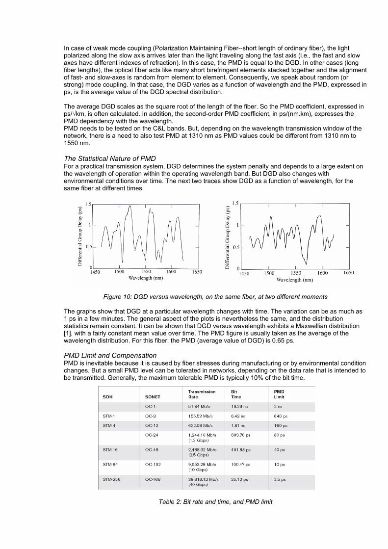
The phase-shift methods are two-ended solutions, allowing measurement through amplifiers on long-haul links. They measure the CD with high accuracy, since the wavelengths of modulated signals are known accurately, and many points of measurements can be acquired, leading to a better fit of the delay curve. However, these solutions are expensive and thus may not be appropriate for metropolitan applications. They require operators at both ends of the link, often with bulky instruments. The pulse-delay methods measure the time that different wavelength carriers travel through the fiber under test, either by photon counting (a direct but very complex method), or by measuring the link length with a multi-wavelength OTDR. The CD-OTDR launches multiple laser pulses into one end of the fiber under test, ideally using more than four different wavelengths for better accuracy. It then analyzes the time to return after a back-reflection from the connector at the other end. The time delay as a function of the wavelength is deduced by comparing the times of flight of the laser pulses.

Figure 8: CD-OTDR principle

Broadband source

Low freq. oscillator

Fiber under test

Delay

Wavelength Tunable filter

transmitter receiver

λ1

λ2

Tunable laser

Reference laser

Low freq. oscillator

Fiber under test

Demux

Delaytransmitter receiver

λ1

λ2

End reflection

The CD-OTDR solution is highly cost-effective, primarily because the initial cost of the instrument is far lower than that of a phase-shift setup. Furthermore, the CD-OTDR is also a complete 3-wavelength OTDR module, which is at the heart of any fiber characterization effort. The CD-OTDR combines two test setups in a single, small instrument. It is a one-ended test solution, resulting in less manpower to carry out the test, less training cost, and lower transportation costs. It can be less accurate than a phase-shift tester, but accuracy better than 5% can be achieved with a 6-wavelength CD-OTDR. This is sufficient to assess a link’s chromatic dispersion, which is a stable and predictable parameter. The CD-OTDR is therefore a good alternative to phase-shift testing in metro rings and regional networks.

Table 1: Comparison table of CD measurement methods Polarization Mode Dispersion (PMD) PMD Definition and Origin Testing for Polarization Mode Dispersion (PMD) is becoming essential before upgrading a network to a higher bit rate because PMD can highly degrade the quality of transmission. It is a difficult parameter to measure, however, because it varies with time and depends on environmental conditions. PMD is known to stem from the difference in the propagation constants of a fiber due to geometrical imperfections in the fiber. The term “PMD” denotes both the physical phenomenon and the associated temporal delay. PMD also causes a system penalty because of the associated pulse spreading in a high-speed digital transmission system. The physical origin of PMD is essentially linear birefringence due to core eccentricity and ovalization. These appear during the manufacturing process or result from external stresses on the fiber, such as bends and twists, and can be considered constant over a length called the “coupling length”. The typical value of the coupling length is several hundred meters and depends on fiber manufacturing parameters. This means that for distances that are practical for transmission applications, the actual length of the fiber is much greater than the coupling length. The PMD phenomenon is characterized by Differential Group Delay (DGD). DGD is the difference in propagation time between the two polarization eigenstates, which are the states of polarization with minimum and maximum propagation time for each wavelength.

Figure 9: DGD of PM and random coupling fibers

Phase-shift method CD-OTDR methodapplication long-haul link metro & access linkmeasurement constraint two-ended measurement one-ended measurement

accuracygood accuracy (depending on number of acquired points) <5% with 6-wavelength CD-OTDR

cost high low + 3-wavelength OTDR testing capability

In case of weak mode coupling (Polarization Maintaining Fiber--short length of ordinary fiber), the light polarized along the slow axis arrives later than the light traveling along the fast axis (i.e., the fast and slow axes have different indexes of refraction). In this case, the PMD is equal to the DGD. In other cases (long fiber lengths), the optical fiber acts like many short birefringent elements stacked together and the alignment of fast- and slow-axes is random from element to element. Consequently, we speak about random (or strong) mode coupling. In that case, the DGD varies as a function of wavelength and the PMD, expressed in ps, is the average value of the DGD spectral distribution. The average DGD scales as the square root of the length of the fiber. So the PMD coefficient, expressed in ps/√km, is often calculated. In addition, the second-order PMD coefficient, in ps/(nm.km), expresses the PMD dependency with the wavelength. PMD needs to be tested on the C&L bands. But, depending on the wavelength transmission window of the network, there is a need to also test PMD at 1310 nm as PMD values could be different from 1310 nm to 1550 nm. The Statistical Nature of PMD For a practical transmission system, DGD determines the system penalty and depends to a large extent on the wavelength of operation within the operating wavelength band. But DGD also changes with environmental conditions over time. The next two traces show DGD as a function of wavelength, for the same fiber at different times.

Figure 10: DGD versus wavelength, on the same fiber, at two different moments The graphs show that DGD at a particular wavelength changes with time. The variation can be as much as 1 ps in a few minutes. The general aspect of the plots is nevertheless the same, and the distribution statistics remain constant. It can be shown that DGD versus wavelength exhibits a Maxwellian distribution [1], with a fairly constant mean value over time. The PMD figure is usually taken as the average of the wavelength distribution. For this fiber, the PMD (average value of DGD) is 0.65 ps. PMD Limit and Compensation PMD is inevitable because it is caused by fiber stresses during manufacturing or by environmental condition changes. But a small PMD level can be tolerated in networks, depending on the data rate that is intended to be transmitted. Generally, the maximum tolerable PMD is typically 10% of the bit time.

Table 2: Bit rate and time, and PMD limit

Since PMD is an unstable phenomenon, it is not easy to compensate for it. However, Dispersion Compensation Modules (DCM) have been developed for that purpose. DCMs are placed in front of receivers on the network and can be tuned in dispersion to compensate for the dispersion measured continuously on a sample of optical pulses. Regularly measuring PMD in the field is essential in order to evaluate network capacity and assess the possibility of upgrading networks for higher bit rate transmission. PMD Measurement Methods In the field, there are three main methods for determining the polarization mode dispersion of an optical fiber, described by three TIA/EIA industry standards: the Fixed Analyzer Method (FOTP-113 standard), the Jones Matrix Method (FOTP-122 standard), and the Interferometric Method (FOTP-124 standard). The fixed analyzer method, also called the wavelength scanning method, involves launching monochromatic polarized light into the fiber under test and measuring the spectral transmission with another polarizer.

Figure 11: Fixed analyzer setup The linear birefringence of a short fiber induces a sinusoidal transmission response when scanning the wavelength.

Figure 12: Wavelength scanning of a short fiber The calculation of PMD on a short fiber is straightforward: it is the inverse of the fringe spacing (in frequency) in the wavelength scanning method. But fiber lengths in networks are much longer than the coupling length. This changes the aspect of the signal obtained, as illustrated in the example below showing a 50 km fiber with a 0.1 ps/ km specific PMD and a 1 km coupling length.

Figure 13: Wavelength scanning of a long fiber

Broadband source Monochromator

Polarizer Polarization controllerFUT

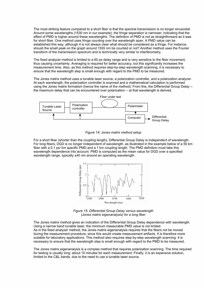
The most striking feature compared to a short fiber is that the spectral transmission is no longer sinusoidal. Around some wavelengths (1530 nm in our example), the fringe separation is narrower, indicating that the effect of PMD is higher around these wavelengths. The definition of PMD is not as straightforward as it was for short fiber. One method uses fringe counting over the wavelength span. A PMD value can be established this way, although it is not always clear what should be considered as a fringe. For instance, should the small peak on the graph around 1555 nm be counted or not? Another method uses the Fourier transform of the transmission spectrum and is technically very similar to interferometry. The fixed analyzer method is limited to a 60 ps delay range and is very sensitive to the fiber movement, thus causing uncertainty. Averaging is required for better accuracy, but this significantly increases the measurement time. Also, as this method requires step-by-step wavelength scanning, it is necessary to ensure that the wavelength step is small enough with regard to the PMD to be measured. The Jones matrix method uses a tunable laser source, a polarization controller, and a polarization analyzer. At each wavelength, the polarization controller is scanned and a mathematical calculation is performed using the Jones matrix formalism (hence the name of the method). From this, the Differential Group Delay -- the maximum delay that can be encountered over polarization -- at that wavelength is derived.

Figure 14: Jones matrix method setup For a short fiber (shorter than the coupling length), Differential Group Delay is independent of wavelength. For long fibers, DGD is no longer independent of wavelength, as illustrated in the example below of a 50 km fiber with a 0.1 ps/ km specific PMD and a 1 km coupling length. The PMD definition must take this wavelength dependence into account. PMD is computed as the mean value for DGD over a specified wavelength range, typically ±40 nm around an operating wavelength.

Figure 15: Differential Group Delay versus wavelength (Jones matrix eigenanalysis) for a long fiber

The Jones matrix method gives an indication of the Differential Group Delay dependence with wavelength. Using a narrow band tunable laser, the minimum measurable PMD value is not limited. As in the fixed analyzer method, the Jones matrix eigenanalysis requires that the fibers not be moved during the measurement procedure, since this would create measurement artifacts. It is therefore more suitable for laboratory applications. This method also requires step-by-step wavelength scanning. It is necessary to ensure that the wavelength step is small enough with regard to the PMD to be measured. The Jones matrix eigenanalysis is a complex method that requires polarization scanning. The time required for testing is usually long: about 10 minutes for each measurement. Finally, it is an expensive solution, limited to the C&L bands, due to the need to use a tunable laser source.

Tunable Laser Source

Polarization controller

Polarimeter

Fiber under test

Computer Differential Group Delay

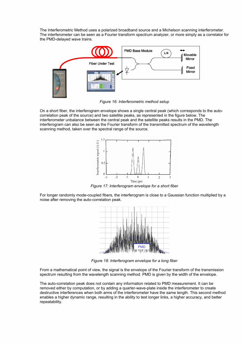
The Interferometric Method uses a polarized broadband source and a Michelson scanning interferometer. The interferometer can be seen as a Fourier transform spectrum analyzer, or more simply as a correlator for the PMD-delayed wave trains.

Figure 16: Interferometric method setup

On a short fiber, the interferogram envelope shows a single central peak (which corresponds to the auto-correlation peak of the source) and two satellite peaks, as represented in the figure below. The interferometer unbalance between the central peak and the satellite peaks results in the PMD. The interferogram can also be seen as the Fourier transform of the transmitted spectrum of the wavelength scanning method, taken over the spectral range of the source.

Figure 17: Interferogram envelope for a short fiber

For longer randomly mode-coupled fibers, the interferogram is close to a Gaussian function multiplied by a noise after removing the auto-correlation peak.

PMDPMDPMD

Figure 18: Interferogram envelope for a long fiber From a mathematical point of view, the signal is the envelope of the Fourier transform of the transmission spectrum resulting from the wavelength scanning method. PMD is given by the width of the envelope. The auto-correlation peak does not contain any information related to PMD measurement. It can be removed either by computation, or by adding a quarter-wave-plate inside the interferometer to create destructive interferences when both arms of the interferometer have the same length. This second method enables a higher dynamic range, resulting in the ability to test longer links, a higher accuracy, and better repeatability.

MovableMirror

FixedMirror

λ/4PMD Base Module

Fiber Under Test

MovableMirror

FixedMirror

λ/4PMD Base Module

Fiber Under Test

This method is well suited for field measurement requirements. The test instruments are rugged and portable, and can operate on batteries. The interferometric method is insensitive to fiber moves. It provides accurate measurements in a few seconds, and does not require averaging. High power broadband sources can be used to increase the dynamic range, allowing measurement of long links up to 250 km. This method also allows PMD measurements through multiple amplifiers such as EDFAs. The minimum measurable PMD value is limited in this method, depending on the spectral width of the broadband source. However, sources with FWHM >50 nm will allow PMD measurement down to 0.05 ps, which is quite acceptable in the field. The interferometric method has been standardized in two versions: the TINTY (traditional interferometry) version, as described above, and the GINTY (generalized interferometry) version. GINTY differs from TINTY by adding polarization scramblers and an analyzer at the input and the output of the fiber under test. This is another way to remove the auto-correlation peak from the interferogram and then measure long links having EDFAs. However, because scramblers are used, averaging a large number of measurements is necessary to achieve the full benefit of this method. As was explained above, technical solutions also exist in the TINTY method to remove this central peak using methods other than computation.

Table 3: Comparison table of PMD measurement methods Conclusion Dispersion in optical fibers limits the quality of signal transmission. Both CD and PMD must be measured to assess the potential of upgrading networks to higher transmission speeds, or to evaluate the need for compensations. Various testing solutions exist, each having advantages and drawbacks. As an aid to finding the most appropriate solution, this paper described the causes and effects of CD and PMD in optical networks and the details of the various testing methods. Related documents [1] F. CURTI et al. "Statistical treatment of the evolution of the principal states of polarization in single-mode fibers" ; Journal of Lightwave Technology, 8, pp. 1162-1166. (1990) [2] ITU-T Recommendation G.650.3 (2007) Test methods for installed single-mode fibre cable sections [3] Chromatic Dispersion Measurement of Optical Fibers by the Phase-Shift Method TIA FOTP-169 (1992; R 1999) [4] Chromatic Dispersion Measurement of Optical Fiber by the Differential Phase-Shift TIA FOTP- 175 (1992) [5] Chromatic Dispersion Measurement of Multimode Graded-Index and Single-mode Optical Fiber by Phase-Shift Method TIA FOTP-168 (1992) [6] Polarization-Mode Dispersion Measurement for Single-Mode Optical Fibers by the Fixed Analyzer Method, draft TIA FOTP-113 (1997) [7] Polarization-Mode Dispersion Measurement for Single-Mode Optical Fibers by Jones Matrix Eigena-nalysis, draft TIA FOTP-122-A (2002) [8] Polarization-Mode Dispersion Measurement for Single-Mode Optical Fibers by the lnterferometric Method, draft TIA FOTP-124-A (2004)

TINTY GINTY

application

any link in the field (measurement through EDFAs possible) laboratory

any link in the field (measurement through EDFAs possible)

any link in the field (measurement through EDFAs possible)

measurement constrainthigh sensitivity to fiber movement

high sensitivity to fiber movementC&L bands only

measurement range 0.08 ps to 60 ps 0.03 ps to 50 ps 0.04 ps to 80 ps 0.04 ps to 115 ps

Dynamic range < 50 dB < 50 dB

> 60 dB (high dynamic both at 1310 nm and 1550 nm) < 50 dB

measurement speedfast for 1 measurement but averaging is required slow fast

fast for 1 measurement but averaging is required

cost low high low low

Interferometric methodsFixed analyzer method Jones matrix method

©2008 Anritsu. All Rights Reserved. ISO 9001:2000 certified. MBCDPMD-WP01-0801-A4