Embed Size (px)
Citation preview
Supporting information on:
Dispersion forces in chirality recognition - a densityfunctional and wave function theory study of diols
Xaiza Aniban,‡a Beppo Hartwig,‡a Axel Wuttke,a Ricardo A. Mataa*
a Institut fur Physikalische Chemie, Georg-August-Universitat Gottingen, Tammannstr. 6, 37077 Gottingen,Germany. E-mail: [email protected]
‡ These authors contributed equally to this work.
Contents
1 DFT data 1
2 WFT data 4
3 Geometry analysis data 53.1 Intermolecular hydrogen bond (A), EDO . . . . . . . . . . . . . . . . . . . . . . . . . . . . . . . . . 53.2 Intermolecular hydrogen bond (A), CHexDO . . . . . . . . . . . . . . . . . . . . . . . . . . . . . . 63.3 Intermolecular hydrogen bond (A), Pinacol . . . . . . . . . . . . . . . . . . . . . . . . . . . . . . . 73.4 Generation of density plots in Figure 4 of the main text. . . . . . . . . . . . . . . . . . . . . . . . . 8
4 Structures 9
References 10
Electronic Supplementary Material (ESI) for Physical Chemistry Chemical Physics.This journal is © the Owner Societies 2021

1 DFT data
0 200 400 600 800 1000 1200tavg(aVQZ) / tavg(XXXX)
0
2
4
6
8
10
E avg
(aVQ
Z) /
kJ m
ol1
DunningVDZaVDZVTZaVTZVQZaVQZAhlrichsdef2-SVPma-def2-SVPdef2-SVPDdef2-TZVP
ma-def2-TZVPdef2-TZVPDdef2-QZVPma-def2-QZVPdef2-QZVPDJensenpcseg-1aug-pcseg-1pcseg-2aug-pcseg-2pcseg-3
0 20 40 60 80 1000.0
0.2
0.4
0.6
0.8
Fig. S1: Overview of the average energy difference relative to the Dunning aVQZ (aug-cc-pVQZ) basis set depend-ing on the fraction of the computational time of aVQZ and each tested basis set. The fully augmentedDunning basis sets (aug-cc-pVXZ) as well as the non augmented variants (cc-pVXZ) were tested[1,2].Furthermore the def2-XZVP Ahlrichs[3] family of basis sets were tested as well as the minamlly aug-mented variants of Zheng et al.[4] and the property optimized heavily augmented variants of Rappoportet al.[5]. Additionally the augmented (aug-pcseg-X) and non augmented (pcseg-X) Jensen basis sets weretested[6]. The aug-pcseg-3 calculations did not converge. All calculations were made for a total of 8different ethanediol dimers and then averaged. For comparable timings each calculation was done on thesame node.
1

Cyclohexanediol
EthanediolPinacol
hom4hom3hom3'
hom3ahom3a'hom3b'hom2''
het4het3het3'
het3b'het2''
9.4 9.8 6.5
7.5 6.4 6.6
6.1 5.5 4.6
8.3 6.6 4.6
8.0 8.8 5.3
8.2 6.0
8.0 8.9
0.0 0.0 0.0
5.4 4.3 3.4
4.9 4.6 2.3
7.5 8.6 3.0
7.6 8.7 6.5
a)no D3(BJ,abc)
Cyclohexanediol
EthanediolPinacol
hom4hom3hom3'
hom3ahom3a'hom3b'hom2''
het4het3het3'
het3b'het2''
10.0 10.4 9.3
11.0 9.7 11.7
9.1 8.8 10.3
13.8 11.5 13.5
13.0 10.4
11.3 12.5 13.9
8.8 11.8
0.0 0.0 0.0
9.3 8.6 7.2
12.9 13.8 9.3
9.9 12.4 11.1
b) D3(BJ,abc)0
2
4
6
8
10
12
0
2
4
6
8
10
12
E0,m
in / kJ mol
1(a) BP86
Cyclohexanediol
EthanediolPinacol
hom4hom3hom3'
hom3ahom3a'hom3b'hom2''
het4het3het3'
het3b'het2''
9.3 6.3
7.4 6.4 7.0
6.0 5.6 5.1
8.4 6.9 5.5
9.1 6.3
7.5 7.9 7.0
7.0 8.7
0.0 0.0 0.0
5.4 4.4 3.8
5.0 4.8 2.8
7.1 8.4 3.3
6.9 8.4 6.5
a)no D3(BJ,abc)
Cyclohexanediol
EthanediolPinacol
hom4hom3hom3'
hom3ahom3a'hom3b'hom2''
het4het3het3'
het3b'het2''
9.8 10.2 8.2
10.0 8.8 10.5
8.1 7.9 8.8
12.2 10.2 10.7
12.0 9.5
9.9 10.9 12.3
7.7 10.6
0.0 0.0 0.0
8.1 6.6
7.9 7.5 6.2
10.6 11.9 7.3
8.6 10.9 9.4
b) D3(BJ,abc)0
2
4
6
8
10
12
0
2
4
6
8
10
12
E0,m
in / kJ mol
1
(b) PBE
Cyclohexanediol
EthanediolPinacol
hom4hom3hom3'
hom3ahom3a'hom3b'hom2''
het4het3het3'
het3b'het2''
8.6 5.4
5.9 5.3 6.2
4.6 4.7 4.8
6.3 5.4 4.4
8.6 5.7
5.4 6.0 6.0
6.0 7.9
0.0 0.0 0.0
3.6 3.1 3.0
3.5 3.9 2.2
4.8 6.4 2.2
5.4 6.7 6.3
a)no D3(BJ,abc)
Cyclohexanediol
EthanediolPinacol
hom4hom3hom3'
hom3ahom3a'hom3b'hom2''
het4het3het3'
het3b'het2''
9.6 9.5 7.0
8.2 7.3 9.2
6.5 6.7 7.8
9.5 8.1 8.9
11.2 9.1
7.1 8.3 10.3
6.3 9.4
0.0 0.0 0.0
6.0 4.9
6.2 6.2 5.1
7.8 9.2 5.5
6.4 8.7 8.7
b) D3(BJ,abc)0
2
4
6
8
10
12
0
2
4
6
8
10
12
E0,m
in / kJ mol
1
(c) PBE0
Cyclohexanediol
EthanediolPinacol
hom4hom3hom3'
hom3ahom3a'hom3b'hom2''
het4het3het3'
het3b'het2''
7.8 4.9
4.1 3.2 3.6
2.9 2.7 2.3
3.9 2.9 0.8
6.1 2.3
3.0 3.2 2.5
6.4 7.5
0.0 0.0 0.7
1.7 1.1 0.7
1.6 1.6 0.0
2.8 3.6 0.0
4.3 5.1 5.4
a)no D3(BJ,abc)
Cyclohexanediol
EthanediolPinacol
hom4hom3hom3'
hom3ahom3a'hom3b'hom2''
het4het3het3'
het3b'het2''
9.7 9.8 7.0
8.2 7.2 8.3
6.5 6.7 7.1
9.1 8.0 7.9
11.1 8.4
6.8 8.0 9.4
7.3 10.6
0.0 0.0 0.0
5.8 4.8 4.8
5.9 5.9 4.2
7.6 8.9 4.9
6.9 9.3 9.6
b) D3(BJ,abc)0
2
4
6
8
10
12
0
2
4
6
8
10
12
E0,m
in / kJ mol
1
(d) B3LYP
Fig. S2: Overview of the DFT results with (b)) and without D3(BJ,abc) (a)) for cyclohexanediol, ethanedioland pinacol. The energies given are always relative to the minimum energy conformer and zero pointcorrected. Grey squares indicate unstable conformers.
2
a) ethanediol
b) cyclohexanediol
c) pinacol
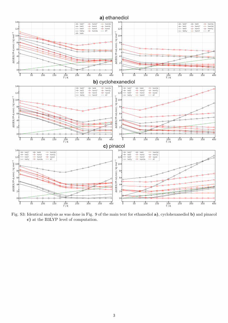
Fig. S3: Identical analysis as was done in Fig. 9 of the main text for ethanediol a), cyclohexanediol b) and pinacolc) at the B3LYP level of computation.
3
2 WFT data
0
2
4
6
8
het-h
om g
ap /
kJ m
ol1
0.0LMP2-d
6.6
0.0LMP2-E
1.9
0.0SCS-d
4.0
0.0SCS-E
4.6
a) ethanediol
0
2
4
6
8
het-h
om g
ap /
kJ m
ol1
0.0LMP2-d
5.3
0.0LMP2-E
1.8
0.0SCS-d
3.1
0.0SCS-E
3.9
b) cyclohexanediol
0
2
4
6
8
het-h
om g
ap /
kJ m
ol1
0.0LMP2-d
7.0
0.0LMP2-E
4.5
0.0SCS-d
5.2
0.0SCS-E
4.2
c) pinacol
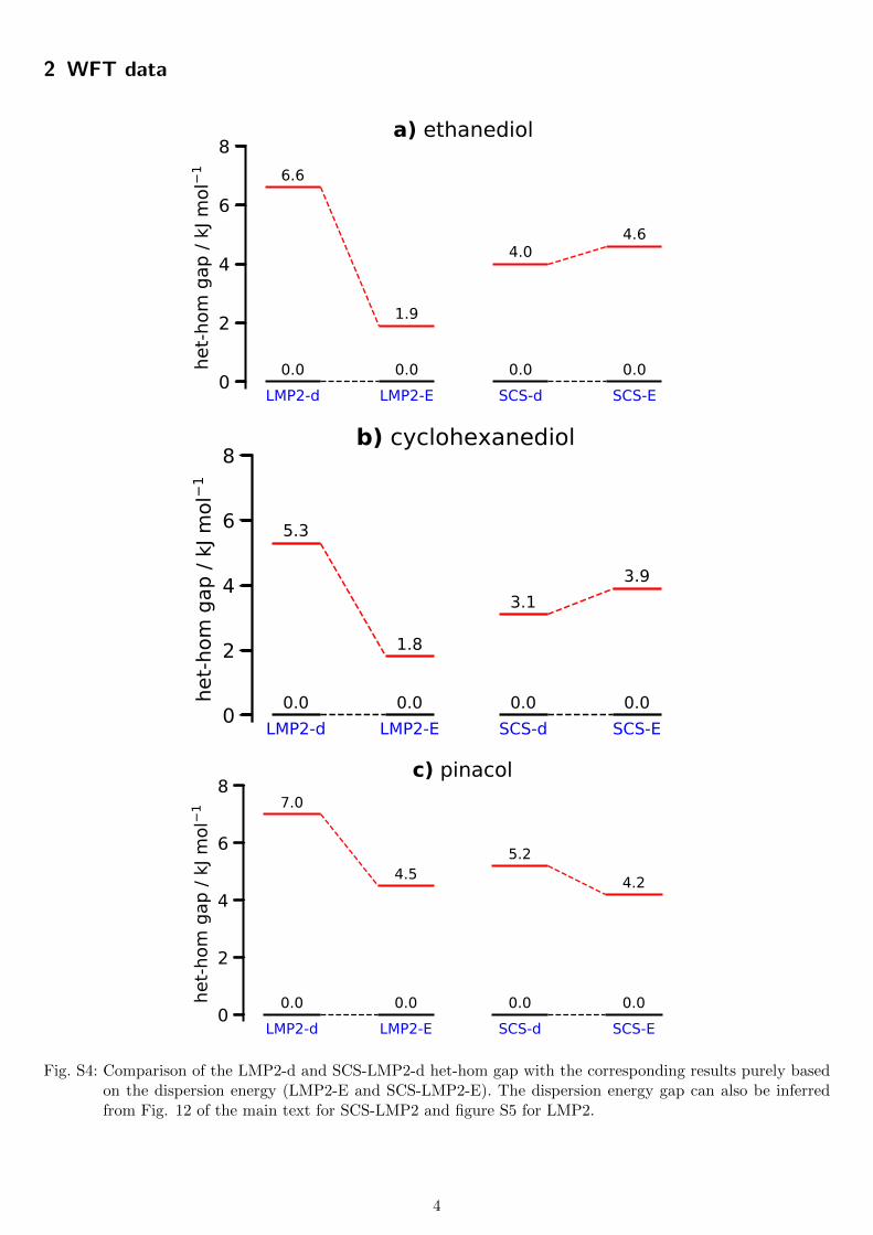
Fig. S4: Comparison of the LMP2-d and SCS-LMP2-d het-hom gap with the corresponding results purely basedon the dispersion energy (LMP2-E and SCS-LMP2-E). The dispersion energy gap can also be inferredfrom Fig. 12 of the main text for SCS-LMP2 and figure S5 for LMP2.
4

het2'
'he
t3 b'he
t3he
t3' het4
hom2''
hom3 b'
hom3
hom3'
hom3a
hom3a
'ho
m4
35
30
25
20
15
10
5
0
E Disp
/ kJ
mol
1
11.2
4.8
12.7
3.5
14.9
4.1
14.1
3.9
18.7
4.9
11.4
4.8
12.8
3.7
14.5
3.7
14.0
4.0
13.1
4.7
13.9
4.1
17.5
4.3
a) ethanediolOH groupsbackbone
het2'
'he
t3 b'he
t3he
t3' het4
hom2''
hom3 b'
hom3
hom3'
hom3a
hom3a
'ho
m4
35
30
25
20
15
10
5
0
E Disp
/ kJ
mol
1
12.3
6.9
13.3
5.1
15.5
5.0
14.6
5.0
19.8
6.2
12.6
7.3
13.7
5.9
15.2
4.9
14.6
5.8
13.3
6.5
18.7
5.5
b) cyclohexanediolOH groupsbackbone
het2'
'he
t3 b'he
t3he
t3' het4
hom2''
hom3 b'
hom3
hom3'
hom3a
hom3a
'ho
m4
35
30
25
20
15
10
5
0
E Disp
/ kJ
mol
1
13.5
9.4
14.5
7.9
15.5
7.9
21.2
9.7
12.9
7.4
15.6
7.9
14.9
8.3
13.2
8.4
17.0
8.2
18.2
8.2
c) pinacolOH groupsbackbone
Fig. S5: Energy fragmentation of the dispersion energy at the LMP2-d level of computation for ethanediol (a)),cyclohexanediol (b)) and pincaol (c)). A zero energy value indicates that a conformer either convergesto a different one or exhibits an imaginary frequency. The performed analysis is analogous to that ofFig. 12 of the main text.
3 Geometry analysis data
3.1 Intermolecular hydrogen bond (A), EDO
Tab. S1: Intermolecular H-bonding optimized at LMP2/aug-cc-pVTZ,H=cc-pVTZ.
Molecular System with dispersion without dispersion
het2” 1.983 1.983 2.133 2.133het3b’ 2.188 2.031 1.892 2.532 2.112 2.000het3 1.905 1.998 1.899 2.045 2.152 2.063het3’ 1.928 1.976 1.920 2.085 2.131 2.100het4 1.959 1.959 1.959 1.959 2.111 2.111 2.111 2.111hom2 1.926 1.973 2.081 2.145hom3a 1.841 1.972 2.065 1.956 2.215 2.244hom3a’ 1.822 1.961 2.021 2.034 3.390 2.046hom3b’ 2.145 1.983 1.886 2.491 2.083 2.006hom3 1.847 1.980 1.959 1.956 2.154 2.136hom3’ 1.876 1.971 1.961 2.004 2.159 2.135
5

Tab. S2: Intermolecular H-bonding optimized at B3LYP/aug-cc-pVTZ,H=cc-pVTZ.
Molecular System with dispersion without dispersion
het2” 1.939 1.939 1.980 1.980het3b’ 2.141 1.988 1.876 2.203 2.046 1.915het3 1.881 1.973 1.865 1.925 2.008 1.911het3’ 1.885 1.943 1.877 1.913 2.000 1.935het4 1.951 1.951 1.951 1.951 1.997 1.997 1.997 1.997hom2” 1.898 1.932 1.957 1.977hom3a 1.810 1.926 2.018 1.832 1.998 2.091hom3a’ 1.792 1.916 2.001 1.811 2.018 2.044hom3b’ 2.062 1.956 1.864 2.114 2.024 1.909hom3 1.828 1.940 1.916 1.852 2.015 1.987hom3’ 1.841 1.935 1.921 1.870 2.019 1.990
Tab. S3: Intermolecular H-bonding optimized at SCS-LMP2/aug-cc-pVTZ,H=cc-pVTZ.
Molecular System with dispersion without dispersion
het2” 2.052 2.052 2.178 2.178het3b’ 2.255 2.083 1.944 2.510 2.152 2.030het3 1.968 2.059 1.964 2.079 2.181 2.096het3’ 1.997 2.038 1.992 2.119 2.161 2.133het4 2.024 2.024 2.024 2.024 2.144 2.144 2.144 2.144hom2” 1.992 2.051 2.116 2.196hom3a 1.897 2.051 2.140 1.987 2.250 2.288hom3a’ 1.866 2.075 2.102 2.063 3.474 2.073hom3b’ 2.232 2.031 1.937 2.499 2.112 2.035hom3 1.900 2.044 2.026 1.986 2.183 2.169hom3’ 1.936 2.039 2.025 2.035 2.188 2.166
3.2 Intermolecular hydrogen bond (A), CHexDO
Tab. S4: Intermolecular H-bonding optimized at LMP2/aug-cc-pVTZ,H=cc-pVTZ.
Molecular System with dispersion without dispersion
het2” 2.002 2.002 2.175 2.175het3b’ 2.176 2.002 1.873 2.378 2.131 2.007het3 1.910 1.988 1.898 2.089 2.139 2.077het3’ 1.960 1.956 1.921 2.140 2.122 2.106het4 1.939 1.939 1.939 1.939 2.099 2.099 2.099 2.099hom2” 2.013 1.947 2.196 2.142hom3a 1.869 1.907 2.065 2.011 2.203 2.301hom3b’ 2.174 1.957 1.880 2.415 2.087 2.024hom3 1.866 1.952 1.942 1.987 2.153 2.159hom3’ 1.923 1.959 1.948 2.055 2.172 2.173
6
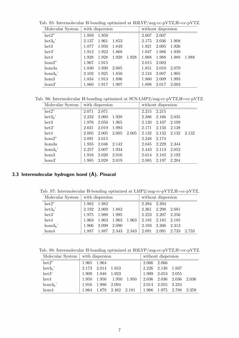
Tab. S5: Intermolecular H-bonding optimized at B3LYP/aug-cc-pVTZ,H=cc-pVTZ.
Molecular System with dispersion without dispersion
het2” 1.959 1.959 2.007 2.007het3b’ 2.137 1.961 1.853 2.175 2.036 1.908het3 1.877 1.950 1.849 1.921 2.005 1.926het3’ 1.912 1.922 1.868 1.947 1.986 1.939het4 1.928 1.928 1.928 1.928 1.988 1.988 1.988 1.988hom2” 1.967 1.915 2.015 2.002hom3a 1.830 1.930 2.005 1.851 2.010 2.079hom3b’ 2.102 1.925 1.850 2.124 2.007 1.905hom3 1.834 1.913 1.896 1.860 2.009 1.993hom3’ 1.860 1.917 1.907 1.898 2.017 2.003
Tab. S6: Intermolecular H-bonding optimized at SCS-LMP2/aug-cc-pVTZ,H=cc-pVTZ.
Molecular System with dispersion without dispersion
het2” 2.071 2.071 2.215 2.215het3b’ 2.232 2.060 1.928 2.386 2.166 2.035het3 1.976 2.050 1.965 2.120 2.167 2.109het3’ 2.031 2.019 1.993 2.171 2.150 2.138het4 2.005 2.005 2.005 2.005 2.132 2.132 2.132 2.132hom2” 2.091 2.015 2.248 2.174hom3a 1.935 2.046 2.142 2.045 2.229 2.344hom3b’ 2.257 2.007 1.934 2.443 2.113 2.052hom3 1.916 2.020 2.016 2.014 2.182 2.192hom3’ 1.985 2.028 2.019 2.085 2.197 2.204
3.3 Intermolecular hydrogen bond (A), Pinacol
Tab. S7: Intermolecular H-bonding optimized at LMP2/aug-cc-pVTZ,H=cc-pVTZ.
Molecular System with dispersion without dispersion
het2” 1.982 1.982 2.394 2.394het3b’ 2.192 2.069 1.883 2.361 2.298 2.081het3’ 1.975 1.980 1.995 2.223 2.207 2.256het4 1.963 1.963 1.963 1.963 2.185 2.185 2.185hom3b’ 1.906 2.099 2.090 2.193 2.306 2.313hom4 1.887 1.887 2.343 2.343 2.091 2.091 2.733 2.733
Tab. S8: Intermolecular H-bonding optimized at B3LYP/aug-cc-pVTZ,H=cc-pVTZ.
Molecular System with dispersion without dispersion
het2” 1.965 1.964 2.066 2.066het3b’ 2.173 2.014 1.853 2.226 2.138 1.937het3’ 1.909 1.948 1.923 1.999 2.053 2.055het4 1.950 1.950 1.950 1.950 2.036 2.036 2.036 2.036hom3b’ 1.916 1.986 2.094 2.014 2.055 2.234hom4 1.864 1.878 2.462 2.181 1.966 1.975 2.788 2.359
7
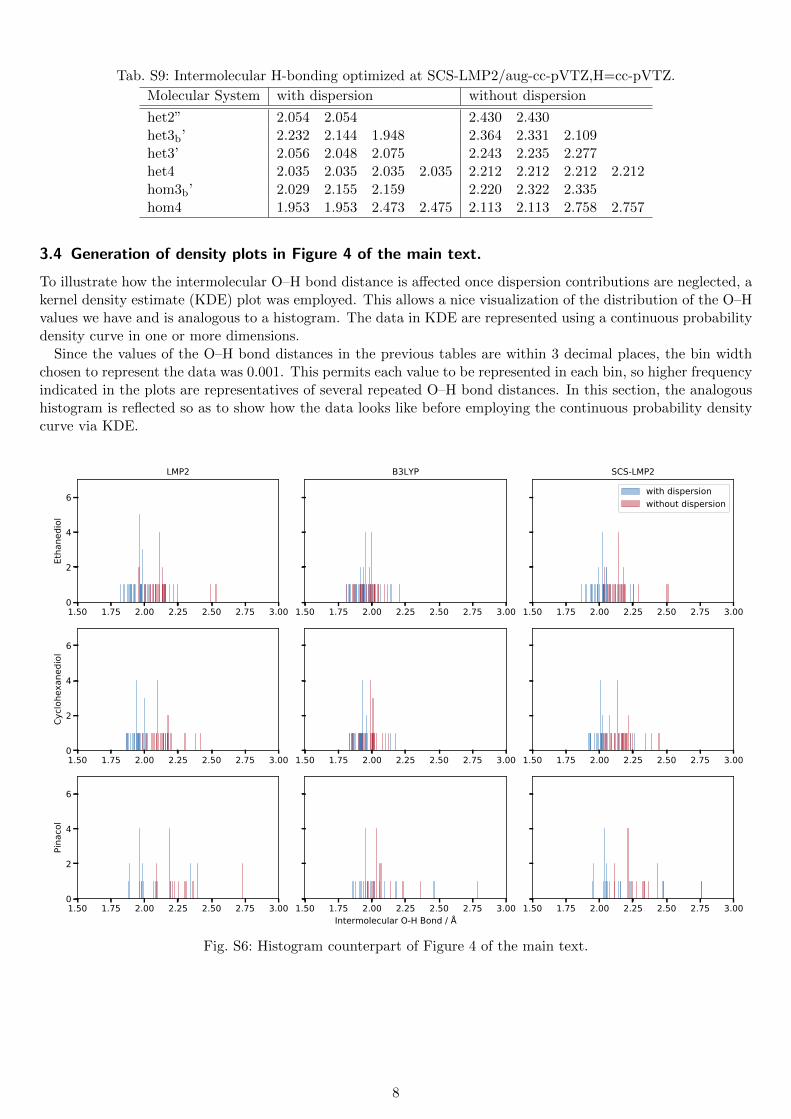
Tab. S9: Intermolecular H-bonding optimized at SCS-LMP2/aug-cc-pVTZ,H=cc-pVTZ.
Molecular System with dispersion without dispersion
het2” 2.054 2.054 2.430 2.430het3b’ 2.232 2.144 1.948 2.364 2.331 2.109het3’ 2.056 2.048 2.075 2.243 2.235 2.277het4 2.035 2.035 2.035 2.035 2.212 2.212 2.212 2.212hom3b’ 2.029 2.155 2.159 2.220 2.322 2.335hom4 1.953 1.953 2.473 2.475 2.113 2.113 2.758 2.757
3.4 Generation of density plots in Figure 4 of the main text.
To illustrate how the intermolecular O–H bond distance is affected once dispersion contributions are neglected, akernel density estimate (KDE) plot was employed. This allows a nice visualization of the distribution of the O–Hvalues we have and is analogous to a histogram. The data in KDE are represented using a continuous probabilitydensity curve in one or more dimensions.
Since the values of the O–H bond distances in the previous tables are within 3 decimal places, the bin widthchosen to represent the data was 0.001. This permits each value to be represented in each bin, so higher frequencyindicated in the plots are representatives of several repeated O–H bond distances. In this section, the analogoushistogram is reflected so as to show how the data looks like before employing the continuous probability densitycurve via KDE.
1.50 1.75 2.00 2.25 2.50 2.75 3.000
2
4
6
Etha
nedi
ol
LMP2
1.50 1.75 2.00 2.25 2.50 2.75 3.00
B3LYP
1.50 1.75 2.00 2.25 2.50 2.75 3.00
SCS-LMP2
with dispersionwithout dispersion
1.50 1.75 2.00 2.25 2.50 2.75 3.000
2
4
6
Cyclo
hexa
nedi
ol
1.50 1.75 2.00 2.25 2.50 2.75 3.00 1.50 1.75 2.00 2.25 2.50 2.75 3.00
1.50 1.75 2.00 2.25 2.50 2.75 3.000
2
4
6
Pina
col
1.50 1.75 2.00 2.25 2.50 2.75 3.00 1.50 1.75 2.00 2.25 2.50 2.75 3.00Intermolecular O-H Bond / Å
Fig. S6: Histogram counterpart of Figure 4 of the main text.
8
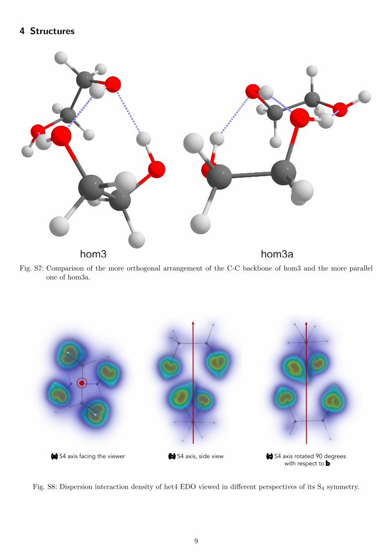
4 Structures
hom3 hom3aFig. S7: Comparison of the more orthogonal arrangement of the C-C backbone of hom3 and the more parallel
one of hom3a.
(a) S4 axis facing the viewer (b) S4 axis, side view (c) S4 axis rotated 90 degreeswith respect to b
Fig. S8: Dispersion interaction density of het4 EDO viewed in different perspectives of its S4 symmetry.
9

References
[1] T. H. Dunning, “Gaussian basis sets for use in correlated molecular calculations. I. The atoms boron throughneon and hydrogen”, J. Chem. Phys. 1989, 90, 1007–1023.
[2] R. A. Kendall, T. H. Dunning, R. J. Harrison, “Electron affinities of the first-row atoms revisited. Systematicbasis sets and wave functions”, J. Chem. Phys. 1992, 96, 6796–6806.
[3] F. Weigend, R. Ahlrichs, “Balanced Basis Sets of Split Valence, Triple Zeta Valence and Quadruple ZetaValence Quality for H to Rn: Design and Assessment of Accuracy”, Phys. Chem. Chem. Phys. 2005, 7, 3297.
[4] J. Zheng, X. Xu, D. G. Truhlar, “Minimally augmented Karlsruhe basis sets”, Theor. Chem. Acc. 2011, 128,295–305.
[5] D. Rappoport, F. Furche, “Property-optimized Gaussian basis sets for molecular response calculations”, J.Chem. Phys. 2010, 133, 134105.
[6] F. Jensen, “Unifying General and Segmented Contracted Basis Sets. Segmented Polarization Consistent BasisSets”, J. Chem. Theory Comput. 2014, 10, 1074–1085.
10