Dispersed fringe tracking with the multi-ro apertures of ...userpages.irap.omp.eu/~lkoechlin/publisenligne/papier RAFT.pdf · L.Koechlin et al. “Dispersed fringe tracking ...”

L.Koechlin et al. “Dispersed fringe tracking ...” 17/04/08 -1-

Dispersed fringe tracking with the multi-roapertures of the Grand Interféromètre à 2 Télescopes

L. Koechlin1, P. R. Lawson2, D. Mourard2, A.Blazit2, D. Bonneau2, F.Morand2, Ph. Stee2,I.Tallon-Bosc3, F.Vakili21 Laboratoire Astrophysique de Toulouse, URA 285 du CNRS, 14 avenue E.Belin 31400 Toulouse, France.2 Observatoire de la Cote d'Azur, Dept. Fresnel, URA 1361 du CNRS, 06460 St. Vallier de Thiey, France.3 Observatoire de Lyon, 9 avenue Charles André, UMR 142 du CNRS, 69561 St Genis Laval Cedex, France.

ABSTRACT

A new fringe tracker based on photon counting detectors and real time image processing has been

implemented on the “Grand Interféromètre à 2 Télescopes” (GI2T) at the Observatoire de la Côte d’Azur. Fringe

visibilities have been recorded on P Cygni and other stars across the Hα emission line with optical path differences

stabilized to between 4 and 7 µm rms (1% of the coherence length). This paper presents the first results and

describes the principle, implementation and performance of the fringe tracker.

Key Words: astronomy, interferometry, fringe tracking

1 . IntroductionThe Grand Interféromètre à 2 Télescopes (GI2T) 1 2 is a long baseline optical stellar

interferometer, located at the Observatoire de Calern, in the Maritime Alps of France. It isnotable for its use of large 1.5 meter apertures, broad multi-channel spectral coverage, beamcombination in the image plane and photon counting cameras. As such, the instrument isunique among stellar interferometers.

Although the GI2T has been operational since 1985 with the largest apertures amongoperational interferometers, up until 1994 fringe acquisition and tracking have been performedvisually. The fringes are contained in dispersed image slices and appear across speckles, eachof which has a limited spatial extent and lifetime. The path-difference is derived from theslope of the dispersed fringes, which are detected even when image slices contain numerousspeckles.

In this paper we describe the automated fringe tracker that has been recentlycommissioned. In Sect. 2 we describe the fringes that are detected in the image plane of theinterferometer. In Sect. 3 we present our method of fringe tracking and in Sect. 4 describe itsimplementation. The performance of the fringe tracker is then discussed and illustrated in Sect.5.


2 Dispersed fringes

We first describe the fringes ignoring atmospheric turbulence and later generalize ourdescription to include atmospheric effects and the use of multi-ro apertures, in which case the

fringes that form in the image plane appear across individual speckles.

2. 1 Dispersed Fringes in the Image Plane

If atmospheric effects are absent, each aperture produces its own diffraction limited imageof the star. As in a Young’s double-slit experiment, the superimposed images are modulatedby fringes, whose spacing depends on the distance between the remapped pupils. For a givenbaseline, the intensity in the combined beam can be written,

I(χ, σ) = Is(σ) [1 + γ cos (2πσ χ + φ)] (1)

where χ is the optical path difference, σ is the spectroscopic wavenumber 1/λ, Is (σ) is the

stellar spectrum, and γ and φ are the modulus and phase of the complex fringe visibility, whichfor resolved stellar sources may be wavelength dependent. Bright fringes are detectedwherever we have

2π σχ + φ = 2kπ , (2)where k is an integer.

In the following we will assume that a grating spectrometer is used to disperse the fringes,as is the case with the GI2T, and that the fringes are imaged onto a detector whose coordinatesare (x,y). The direction of dispersion is made parallel to the x axis, such that we have λ = a x ,

(3)

where a is proportional to the dispersion coefficient of the grating. We also assume that thedirection of dispersion is perpendicular to the remapped pupil separation, so that the path-difference χ is only a function of y. We have therefore

χ = χo - b y , (4)

where b depends on the pupil separation and the distance to the image plane, and χo is theoptical path-difference at the center of the image. Equation (2) then becomes

2πχ 0 − byax + φ= 2kπ

, (5)

which yields the equation of the fringes on the detector. The spectrum therefore contains a set


of diverging bright fringes whose paths are described by

(k − φ /2π) ax + by − χ 0 = 0 . (6)

The path difference due to the piston phase determines the origin yo = χo / b of the fringes

on the y axis, as well as their slope on the detector. As sketched on Figure 1, the slope of thefringes in the field indicates both the sign and magnitude of the path-difference χo . If we set b

= 0 then equation (6) also describes a channeled spectrum.

spectrometer slit(zero order)y

x

k = 0

k = 7

k = 8

- xo/b

fringes

dispersed image (first order)on the field of the detector

k = 1

Figure 1. Dispersed fringes follow the equation of a set of diverging lines.

The rectangular shaded area corresponds to the dispersed image field.

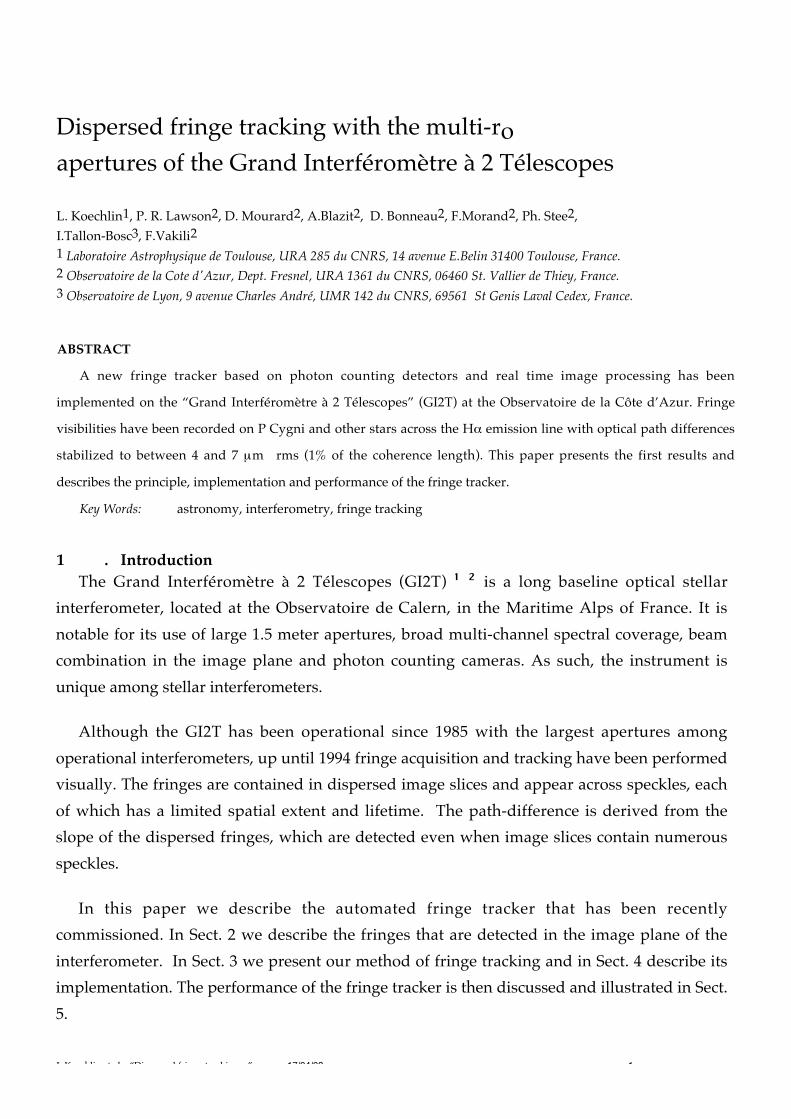
Figure 2. Photograph of a dispersed image of a fringe pattern across a star.


2. 2 Dispersed Fringes using Multi-ro apertures

With multi-ro, apertures the effects of atmospheric turbulence across individual apertures

cause the dispersed fringe pattern to be separated into numerous speckles as shown on Figure2. Large scale phase variations further limit fringe measurements to a confined coherencevolume, encompassing spatial, temporal, and chromatic phase changes.

Although each speckle contains a fringe pattern described in Eq. (1), fringes of differentspeckles have different phase relationships and therefore cannot be coherently combined. Theaverage delay is derived from the integrated power spectra of individual fringed speckles, andthe speckles must be processed individually in each frame. An image slicer is therefore used,whose slits’ width corresponds to the speckle size; the detected spectrum shows the spectra ofnumerous speckles, but each is separated vertically at different locations in the image slice.

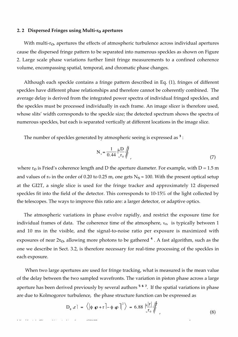
The number of speckles generated by atmospheric seeing is expressed as 3 :

Ns =

10.44

äãåå Dr0 ëíìì2 , (7)

where ro is Fried’s coherence length and D the aperture diameter. For example, with D = 1.5 m

and values of ro in the order of 0.20 to 0.25 m, one gets Ns ≈ 100. With the present optical setup

at the GI2T, a single slice is used for the fringe tracker and approximately 12 dispersedspeckles fit into the field of the detector. This corresponds to 10-15% of the light collected bythe telescopes. The ways to improve this ratio are: a larger detector, or adaptive optics.

The atmospheric variations in phase evolve rapidly, and restrict the exposure time forindividual frames of data. The coherence time of the atmosphere, τo, is typically between 1and 10 ms in the visible, and the signal-to-noise ratio per exposure is maximized with

exposures of near 2τo, allowing more photons to be gathered 4 . A fast algorithm, such as the

one we describe in Sect. 3.2, is therefore necessary for real-time processing of the speckles ineach exposure.

When two large apertures are used for fringe tracking, what is measured is the mean valueof the delay between the two sampled wavefronts. The variation in piston phase across a large

aperture has been derived previously by several authors 5 6 7. If the spatial variations in phaseare due to Kolmogorov turbulence, the phase structure function can be expressed as

Dφ ár é = φ áρ + r é− φ áρ é 2 = 6.88 äãåå r

r0

ëíìì53

, (8)


where ro is Fried’s coherence length and r is an arbitrary separation between two points in the

average wave plane. If the wavefront tilt is not compensated, the mean squared variations afterpiston phase is removed, measured over a diameter D, can be shown to be

φ2rms = 1.03 äãåå D

r0

ëíìì53

. (9)This is approximately true for the apertures of the GI2T, which is not presently equipped

with adaptive optics, and whose star tracker corrects tilt up to 0.5 Hz. For the GI2T, theobserved path variance is therefore twice as large as in eq. (9) and the rms spread is √2 timesthe above. The rms path difference is therefore

Δχ rms = 0.229 λ äãåå Dr0

ëíìì56

. (10)

For an ro of 0.2 m and apertures of 1.5 m diameter, the rms variations in the visible are

about 0.75 µm. The use of adaptive optics would reduce the numerical coefficient in eq. (9) (Seetable IV in reference 6.) For example, with the tilt completely removed the rms variations inpath length become close to 0.25 µm. However, it would be difficult to stabilize a fringe patternto better than λ/4, which requires the aberrations from the first ten Zernicke polynomials to becorrected. It follows that although it is possible for light from two large apertures to becombined coherently, the resolution in delay tracking is limited by the aperture size.

2. 3 Coherence Envelope and Tracking Resolution

To record the fringes at the GI2T, a spectrometer is used in conjunction with a 2D photon-counting array detector. The spatial information contained in the fringes is modified throughthe process of detection. Thus in the direction of dispersion the response is a convolution of theoptical point spread functions of the spectrometer and detector. The power spectrum of thisresponse determines the sensitivity to fringes as a function of path-difference. If the resolutionis limited by sampling, the coherence length is determined by the bandwidth per pixel. If abandwidth of Δσ is dispersed across N spectral channels, then each channel represents a

bandwidth of Δσ/N and therefore a coherence length of N/Δσ, or approximately Nλ2/ Δλ.Dispersing a large bandwidth in this way increases the coherence length by a factor of N.Losses may also occur due to sampling in the direction perpendicular to the dispersion, wherethe fringe spacing at red wavelengths may be larger than those at blue wavelengths. Thisspacing is determined by the remapped pupil separation and is a constant during theobservations. It is therefore possible to choose a suitable separation and over-sample the redfringes, so that losses in the blue are rendered negligible.


Another consequence of the detection is that the spectrum is truncated, or windowed; the

resolution in path-difference is limited by the Fourier transform of this window function 8 .The resolution is inversely proportional to the total detected bandwidth, and limited by thephoton noise. By interpolation in the Fourier plane, the precision in the measurement of thepath length difference χ can approach a fraction of a wavelength.

Fringe trackers may be broadly characterized by their ability to maintain the optical pathdifference equal to within a small fraction of the wavelength (λ), or within only a fraction of thecoherence length (λ2/Δλ). These modes are respectively referred to as cophasing and

coherencing 9 . Cophasing keeps stabilized fringes visible at any exposure time. Coherencinglets phase fluctuations blur the fringes at long exposures.

Although in principle a system based on dispersed fringe tracking is capable of cophasingan interferometer, cophasing is only possible when the phase variations across each apertureare compensated to less than a fraction of a wavelength. For a multi-ro aperture this wouldrequire some form of adaptive optics.

3 Principle of fringe tracking

3.1 Method of Delay Estimation

The optical delay in the center of the dispersed fringe image is sampled and used as anerror signal for the fringe tracker control loop. Fringe slope and optical delay are related to oneanother by a linear relation, derived from equation (6) in the following.

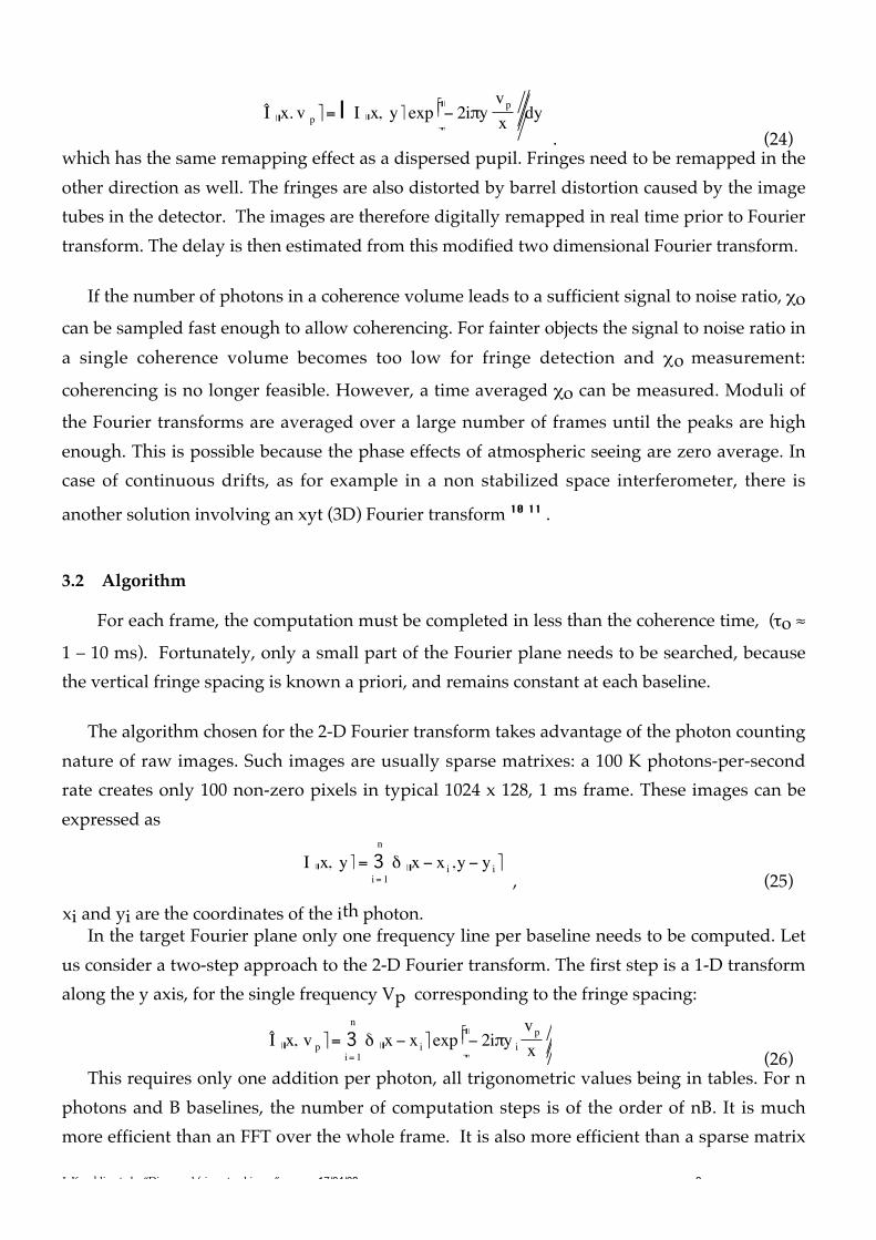
On Figure 3. the optical delay χo is different from zero and fringes appear tilted. Δλ and δλ

are respectively the total bandpass and the spectral fringe spacing. Δy and δy are respectivelythe vertical extent of the field and the vertical fringe spacings. The object phase φ is consideredconstant over the spectral bandpass and can therefore be omitted in the following.

For points (λ1, y1) and (λ1, y1+δy) on two adjacent fringes, relation (6) yields

kλ1 + by1 = χo , (11)

(k+1 )λ1+ b (y1+δy) = χo . (12)

Subtracting the above expressions, the vertical fringe spacing δy can be expressed:δy = λ 1 / b . (13)

In the dispersion direction, for points (λ1, y1) and (λ1 -δλ, y1) on two neighboring fringes,


relation (6) becomeskλ1+ by1 = χo , (14)

(k+1) (λ1 - δλ) + by1 = χo , (15)Subtracting the above expressions yields

δλ = λ 1 / k . (16)At this point, fringe number k can be expressed as k = (χo - by1)/ λ1 , we have therefore

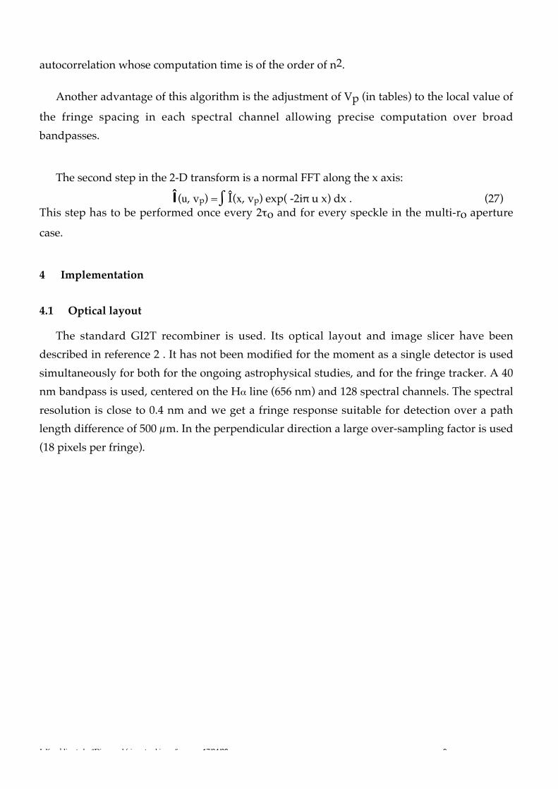
δλ = λ 21 / áχ 0 − by1 é , (17)The Fourier transform of such a quasi-periodic fringe pattern will show peaks at

frequencies (Up , Vp) and (-Up , -Vp ), such as on Figure 4. As the total field in the source imageis (∆x, Δy) , and assuming a constant fringe spacing over the field, the relation between Upand δλ is the following:

Up = Δx / δx = Δλ / δλ , (18)

therefore, from equation (17)U p = áχ 0 − by1 é ∆λ /λ 2

. (19)The path length difference: χ = χ0 - by , varies slightly with the vertical position in the image.

The corresponding spread in the discretized Fourier space is negligible if:

Δχmax <λ2 / Δλ , (20)where Δχmax is the maximum path length variation across the image field. This is the case

with the present GI2T recombiner. Equation (19) then becomes

χ 0 . Up λ 2 /∆λ . (21)This relation is used to derive the sign and amplitude of the optical delay in the

interferometer. The relation does not depend on the sampling nor on any instrumental settingother than the wavelength and the total bandpass (Δλ) used.

The spatial frequency in the perpendicular direction is given by:Vp = Δy / δy = b Δy / λ1 . (22)

Vp is not dependent upon the optical delay χo . However, Up and Vp are wavelength

dependent. In a broad band field, fringes are not equally spaced and parallel, and a twodimensional Fourier transform would not yield optimal results. One optical solution that hasbeen thought of is a dispersed pupil: if the distance between remapped apertures in the pupilis made proportional to the wavelength, the fringe slope becomes wavelength independent.The solution presently implemented is numerical. The first step in a 2D Fourier transformwould be the expression

I áx. v p é = I I áx, y é exp á− 2iπy v p é dy . (23)

It is here replaced by


I áx. v p é = I I áx, y é exp äãåå− 2iπyvp

xëíììdy

. (24)which has the same remapping effect as a dispersed pupil. Fringes need to be remapped in theother direction as well. The fringes are also distorted by barrel distortion caused by the imagetubes in the detector. The images are therefore digitally remapped in real time prior to Fouriertransform. The delay is then estimated from this modified two dimensional Fourier transform.

If the number of photons in a coherence volume leads to a sufficient signal to noise ratio, χocan be sampled fast enough to allow coherencing. For fainter objects the signal to noise ratio ina single coherence volume becomes too low for fringe detection and χo measurement:

coherencing is no longer feasible. However, a time averaged χo can be measured. Moduli of

the Fourier transforms are averaged over a large number of frames until the peaks are highenough. This is possible because the phase effects of atmospheric seeing are zero average. Incase of continuous drifts, as for example in a non stabilized space interferometer, there is

another solution involving an xyt (3D) Fourier transform 10 11 .

3.2 Algorithm

For each frame, the computation must be completed in less than the coherence time, (τo ≈

1 – 10 ms). Fortunately, only a small part of the Fourier plane needs to be searched, becausethe vertical fringe spacing is known a priori, and remains constant at each baseline.

The algorithm chosen for the 2-D Fourier transform takes advantage of the photon countingnature of raw images. Such images are usually sparse matrixes: a 100 K photons-per-secondrate creates only 100 non-zero pixels in typical 1024 x 128, 1 ms frame. These images can beexpressed as

I áx, y é = n

3i= 1δ áx − xi ,y − yi é

, (25)

xi and yi are the coordinates of the ith photon.In the target Fourier plane only one frequency line per baseline needs to be computed. Let

us consider a two-step approach to the 2-D Fourier transform. The first step is a 1-D transformalong the y axis, for the single frequency Vp corresponding to the fringe spacing:

I áx, v p é = n

3i= 1δ áx − xi é exp äãåå− 2iπy i

vp

xëíìì (26)

This requires only one addition per photon, all trigonometric values being in tables. For nphotons and B baselines, the number of computation steps is of the order of nB. It is muchmore efficient than an FFT over the whole frame. It is also more efficient than a sparse matrix


autocorrelation whose computation time is of the order of n2.

Another advantage of this algorithm is the adjustment of Vp (in tables) to the local value of

the fringe spacing in each spectral channel allowing precise computation over broadbandpasses.

The second step in the 2-D transform is a normal FFT along the x axis:

Î(u, vp) = ∫ Î(x, vp) exp( -2iπ u x) dx . (27)This step has to be performed once every 2τo and for every speckle in the multi-ro aperture

case.

4 Implementation

4.1 Optical layout

The standard GI2T recombiner is used. Its optical layout and image slicer have beendescribed in reference 2 . It has not been modified for the moment as a single detector is usedsimultaneously for both for the ongoing astrophysical studies, and for the fringe tracker. A 40nm bandpass is used, centered on the Hα line (656 nm) and 128 spectral channels. The spectralresolution is close to 0.4 nm and we get a fringe response suitable for detection over a pathlength difference of 500 µm. In the perpendicular direction a large over-sampling factor is used(18 pixels per fringe).


δy = vertical fringe spacing

Grating

λ= ax

Δλ

Combined focus

Dispersed Speckle

spectral fringe spacing

= a δx = δ λ

y

slit

y1

λ1

Δy

Fringe k

Fringe k+1

Figure 3. Fringes in a dispersed speckle in the image plane.


UpU

V

Vp

Figure 4. Peaks in the Fourier transform of the dispersed fringe image. The spatial frequency Up

is related to the optical delay by the expression Up = co (Dl / l2) , where co is the optical path length at

the center of the image.

4.2 Detectors and Data Acquisition

The dispersed image plane is sampled by a photon counting detector: the CP40 12 . TheCP40 is an intensified CCD camera with an extended-red S20 photocathode. An average of 250x 600 pixels are used in the present setup. The detective quantum efficiency of this detectorpeaks at approximately 5.5%. It can operate to a maximum flux of 1200 photons per frame,limited by the camera digital electronics, and provides a fixed frame rate of 20 ms. A Ranicon

detector 13 has also been used to allow the frame rate to be adjusted to the seeing conditions.This camera has been helpful in the implementation stage, but it is not used for fringe tracking,

due to a limitation in photon flux (1.5x104 photons/s).

Once detected, photon coordinates are sent to computers: a RISC processor Macintosh forthe real time optical delay computing and control, and HP workstations for data storage andoff-line fringe visibility processing.

4.3 Control

The variance of the integrated modulus as a function of spatial frequency is sampled andcompared to the peak value. When the signal reaches a given threshold, which may take froma few 20 ms frames to a few seconds, depending on the stellar visibility and magnitude, the


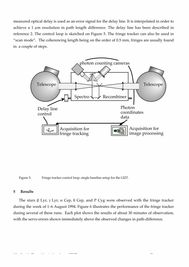
measured optical delay is used as an error signal for the delay line. It is interpolated in order toachieve a 1 µm resolution in path length difference. The delay line has been described inreference 2. The control loop is sketched on Figure 5. The fringe tracker can also be used in“scan mode”. The coherencing length being on the order of 0.5 mm, fringes are usually foundin a couple of steps.

Telescope

Recombiner

Telescope

Acquisition for fringe tracking

Acquisition forimage processing

Delay line control

Photon coordinates data

photon counting cameras

Spectro

Figure 5. Fringe tracker control loop: single baseline setup for the GI2T.

5 Results

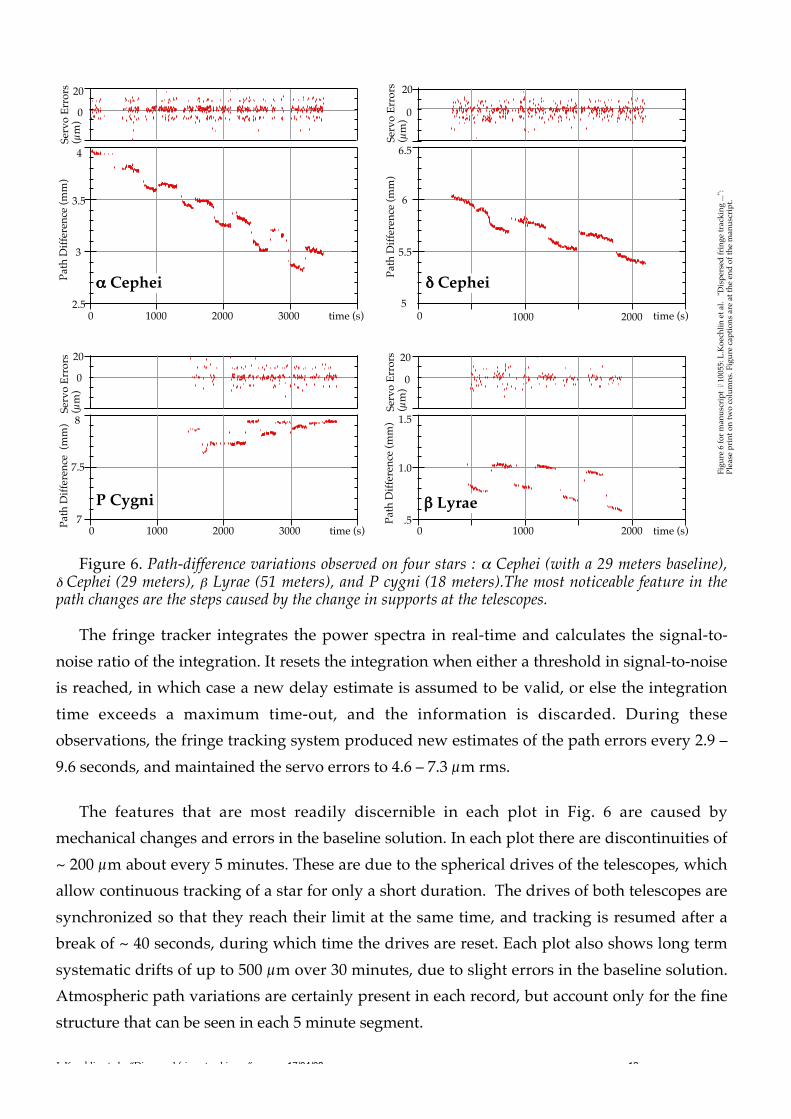
The stars β Lyr, γ Lyr, α Cep, δ Cep, and P Cyg were observed with the fringe trackerduring the week of 1–6 August 1994. Figure 6 illustrates the performance of the fringe trackerduring several of these runs. Each plot shows the results of about 30 minutes of observation,with the servo errors shown immediately above the observed changes in path-difference.


Serv

o Er

rors

(µ

m)

0 1000 2000 time (s)

Serv

o Er

rors

(µ

m)

0

20

Path

Diff

eren

ce (m

m)

2.5

3

3.5

4

0 1000 2000 3000

0

20

Path

Diff

eren

ce (

mm

)

Path

Diff

eren

ce (m

m)

Path

Diff

eren

ce (m

m)

time (s)

α Cephei

Serv

o Er

rors

(µ

m)

Serv

o Er

rors

(µ

m)

0 1000 2000 3000 time (s)

P Cygni

0

20

7

7.5

8

5

5.5

6

6.5

.5

1.0

1.5

0

20

0 1000 2000 time (s)

δ Cephei

β Lyrae

Figu

re 6

for m

anus

crip

t # 1

0055

: L.K

oech

lin e

t al.

"D

ispe

rsed

frin

ge tr

acki

ng ..

.":

Plea

se p

rint o

n tw

o co

lum

ns. F

igur

e ca

ptio

ns a

re a

t the

end

of t

he m

anus

crip

t.

Figure 6. Path-difference variations observed on four stars : α Cephei (with a 29 meters baseline),δ Cephei (29 meters), β Lyrae (51 meters), and P cygni (18 meters).The most noticeable feature in thepath changes are the steps caused by the change in supports at the telescopes.

The fringe tracker integrates the power spectra in real-time and calculates the signal-to-noise ratio of the integration. It resets the integration when either a threshold in signal-to-noiseis reached, in which case a new delay estimate is assumed to be valid, or else the integrationtime exceeds a maximum time-out, and the information is discarded. During theseobservations, the fringe tracking system produced new estimates of the path errors every 2.9 –9.6 seconds, and maintained the servo errors to 4.6 – 7.3 µm rms.

The features that are most readily discernible in each plot in Fig. 6 are caused bymechanical changes and errors in the baseline solution. In each plot there are discontinuities of~ 200 µm about every 5 minutes. These are due to the spherical drives of the telescopes, whichallow continuous tracking of a star for only a short duration. The drives of both telescopes aresynchronized so that they reach their limit at the same time, and tracking is resumed after abreak of ~ 40 seconds, during which time the drives are reset. Each plot also shows long termsystematic drifts of up to 500 µm over 30 minutes, due to slight errors in the baseline solution.Atmospheric path variations are certainly present in each record, but account only for the finestructure that can be seen in each 5 minute segment.


The plot of P Cygni is the most remarkable in this series. It has a V magnitude of 4.8 and isthe second faintest object for which fringes have ever been tracked with the GI2T – the faintestobject being HR 7132 with a V magnitude of 5.6 (observed with a baseline of 16.3 m on June 7,1995). During the observation in Fig. 7(d) the fringe tracker maintained the paths equal to 5.1µm rms and produced estimates every 5.7 s on average, which is comparable to itsperformance with much brighter stars.

6 Remarks

Theoretical predictions suggested that if fringes could be observed using all the collected

light on large telescopes 14 15 , a limiting magnitude would be reached between 13 and 17 with

1.5 m apertures. While 17th magnitude has been reached by speckle interferometry on a 3.6 m

telescope 16, no long baseline optical interferometer has ever observed objects much fainter

than 5th magnitude. The reason for this disparity is that interferometers must track fringes tomaintain coherence between the apertures. The path-difference must be continuouslymeasured and corrected.

The advantage of a multi-ro aperture is that it allows a larger number of coherence areas to

be sampled at the same time. For a large aperture, this in principle leads to an improvementproportional to the diameter D in the signal-to-noise ratio, but the field and processing power

requirements increase with D2 . The slow development of an automated system for the GI2Thas mainly been due to the lack of an adequate algorithm and sufficient computing power. Thepresent recombiner samples approximately 12 speckles under the seeing conditions specifiedin section 2.2, and yields a gain of 3.5 in the signal-to-noise ratio over a comparable single-ro

system. At low light level conditions, the signal-to-noise ratio is proportional to the photonflux (see reference 15). Therefore in terms of limiting magnitude, this is a gain of 1.5 . Thewhole speckle pattern on a 1.5 m telescope, if analyzed, would yield a gain of 10 in the signal-to-noise ratio (2.5 magnitudes). Other parameters such as the optical throughput, the detectorefficiency, and the angular extent of the observed objects, are responsible for the gapremaining between theoretical and observational limits.

As the aperture size increases, the transfer function of the instrument causes the fringesignal to spread out in the spatial frequency domain. The resulting loss has been noted by

several authors 17 18 . This problem is overcome by integrating – around – , the peak of the

fringe signal, rather than sampling the peak height 19 and that is done automatically by thefringe tracker.


7 Conclusion

The new fringe tracker of the GI2T currently provides correction for path-variations with anaccuracy of ≈ 5 µm rms. It takes advantage of the interferometer's large apertures andrelatively broad spectral bandpass (40 nm) without constraining the coherence length. It hasbenefited the instrument by providing rapid fringe acquisition, and, as demonstrated by theobservations of P Cygni and HR 7132, an extended limiting magnitude.

We have shown that despite the lack of adaptive optics in the GI2T, it is yet possible to takeadvantage of multi-ro apertures to track fringes in dispersed stellar spectra. This method hasthe potential of enhancing the performance of future large telescopes arrays, either multi-speckle, or diffraction limited. It has already allowed the GI2T to track on objects that, to theauthors’ knowledge, are fainter than those observed by any other stellar interferometer.

Acknowledgments

The authors are grateful for the help of Antoine Labeyrie, Luc Arnold, Guy Merlin, andJean Pinel. They are also thankful to Francesco Paresce, Knute Ray, and Colin Cox for theirhelp with the Ranicon detector. LK acknowledges the support of funding from the theProgramme National de Haute Résolution Angulaire en Astrophysique and the Groupe DeRecherches Milieux circum-stellaires. PRL was funded in this study by the Centre National deRecherche Scientifique and the Conseil Général des Alpes Maritimes through an HenriPoincaré Fellowship at the Observatoire de la Cote d’Azur. The GI2T is maintained andoperated with the support of the Programme National de Haute Résolution Angulaire enAstrophysique.

When this work was performed P.R. Lawson was with the Observatoire de la Cote D'Azur.He is now with the Mullard Radio Astronomy Observatory, Cavendish Laboratory, MadingleyRoad, Cambridge CB3 0HE, UK.


References

1 A. Labeyrie, G. Schumacher, M. Dugué, C. Thom, F. Foy, D. Bonneau, and R. Foy, “Fringes

obtained with the large boule interferometer at CERGA,” Astron. Astrophys. 162, 359-364

(1986).

2 D. Mourard, I. Tallon-Bosc, A. Blazit, D. Bonneau, G. Merlin, F. Morand, F. Vakili, and A.

Labeyrie, “The GI2T interferometer on Plateau de Calern,” Astron. Astrophys. 283, 705-713

(1994).

3 C.Aime, “Measurement of averaged squared modulus of atmospheric-lens modulation

transfer function”J. Opt. Soc. Am. 64, 1129-1132 (1974)

4 F. Roddier, “Atmospheric limitations to high angular resolution imaging,” in ESO

Conference Proc. on “Scientific Importance of High Angular Resolution at Infrared and Optical

Wavelengths,” (ESO: Garching, 1981) pp. 5-23.

5 D.L. Fried, “Statistics of a geometric representation of wavefront distortion,” J. Opt. Soc. Am.

55, 1427-1434 (1965).

6 R.J. Noll, “Zernike polynomials and atmospheric turbulence,” J. Opt. Soc. Am. 66, 207-211

(1976).

7 R.A. Sasiela, Electromagnetic Wave Propagation in Turbulence, (Springer - Verlag: Berlin,

1994), pp. 63-65.

8 P. R. Lawson, “Group delay tracking in optical stellar interferometry using the Fast Fourier

Transform,” J. Opt. Soc. Am. A. 12 , 366-374 ( 1995).

9 J.M. Beckers, “Cophasing telescope arrays,” in Difffraction-Limited Imaging with Very Large

Telescopes , D.M. Alloin and J.M. Mariotti eds., (Kluwer: Dordrecht 1989) pp. 355-34.

10 L. Koechlin, “The I2T interferometer,” in High Resolution Imaging by Interferometry, J. M.


Beckers ed., (European Southern Observatory, Garching bei München, 1988) pp. 695-704.

11 L. Koechlin, “Active fringe tracking,” in – High Resolution Imaging by Interferometry II, –

J.M. Beckers and F. Merkle, ed. (European Southern Observatory, Garching bei München,

1992) pp. 1239--1246.

12 A. Blazit "A 40mm photon counting camera" in proceedings of “Image Detection and

Quality”, Proc. Soc. Photo-Opt. Instrum. Eng. p. 259-263 (1986).

13 M. Clampin, J. Crocker, F. Paresce, M. Rafal “Optical Ranicon detectors for photon counting

imaging. I.” Review of Scientific Instruments, 59, 8, p. 1269-1285 (1988).

14 A. Labeyrie, “Stellar interferometry methods,” Ann. Rev. Astron. Astrophys. 16, 77-102

(1978).

15. F.Roddier and P.Léna “ Long baseline Michelson interferometry with large ground-based

telescopes operating et optical wavelengths” J.Optics (Paris) 15, 4, p. 171-182 (1984)

16 R. Foy, D. Bonneau, A. Blazit, “The multiple QSO PG1115 +08: A fifth component.” Astron.

Astrophys. 149, L13-L16 (1985).

17 W. J. Tango and R. Q. Twiss, “Michelson stellar interferometry,” Prog. Opt. 17, 239-277

(1980).

18 D. Buscher, “Optimizing a ground-based optical interferometer for sensitivity at low light

levels,” Mon. Not. R. Astr. Soc. 235, 1203-1226 (1988).

19 D. Mourard, I. Tallon-Bosc, F. Rigal, F. Vakili, D. Bonneau, F. Morand, and Ph. Stee,

“Estimation of visibility amplitude by optical long-baseline Michelson stellar interferometry

with large apertures”, Astron. Astrophys. 288, 675--682 (1994).

Documents

Dispersed fringe tracking with the multi-ro apertures of ...userpages.irap.omp.eu/~lkoechlin/publisenligne/papier RAFT.pdf · L.Koechlin et al. “Dispersed fringe tracking ...”