Dispatch of Bulk Energy Storage in Power Systems with

Wind Generation

by

Samir Gupta

A Thesis Presented in Partial Fulfillment

of the Requirements for the Degree

Master of Science

Approved April 2012 by the

Graduate Supervisory Committee:

Gerald Heydt, Chair

Vijay Vittal

Raja Ayyanar

ARIZONA STATE UNIVERSITY

May 2012

i

ABSTRACT

This thesis concerns the impact of energy storage on the power system.

The rapidly increasing integration of renewable energy source into the grid is

driving greater attention towards electrical energy storage systems which can

serve many applications like economically meeting peak loads, providing spin-

ning reserve. Economic dispatch is performed with bulk energy storage with wind

energy penetration in power systems allocating the generation levels to the units

in the mix, so that the system load is served and most economically. The results

obtained in previous research to solve for economic dispatch uses a linear cost

function for a Direct Current Optimal Power Flow (DCOPF). This thesis uses

quadratic cost function for a DCOPF implementing quadratic programming (QP)

to minimize the function. A Matlab program was created to simulate different test

systems including an equivalent section of the WECC system, namely for Arizo-

na, summer peak 2009.

A mathematical formulation of a strategy of when to charge or discharge

the storage is incorporated in the algorithm. In this thesis various test cases are

shown in a small three bus test bed and also for the state of Arizona test bed. The

main conclusions drawn from the two test beds is that the use of energy storage

minimizes the generation dispatch cost of the system and benefits the power sys-

tem by serving the peak partially from stored energy. It is also found that use of

energy storage systems may alleviate the loading on transmission lines which can

defer the upgrade and expansion of the transmission system.

ii

ACKNOWLEDGEMENTS

I would like to first and foremost offer my sincerest gratitude to my advi-

sor, Dr. Gerald T. Heydt, whose encouragement, guidance and support from the

initial to the final level enabled me to develop an understanding of the subject. I

attribute the level of my Master’s degree to his encouragement and effort and

without him this thesis, too would not have been completed. One simply could not

wish for a friendlier supervisor. I also want to express my gratitude to Dr. Vijay

Vittal and Dr. Raja Ayyanar for their time and consideration in being a part of my

graduate supervisory committee.

Financial assistance provided by the Power Systems Engineering Research

Center (PSERC), a National Science Foundation Industry-University Cooperative

Research Center, is greatly acknowledged (under award EC 0968883).

I especially want to thank my parents Mr. Satish K. Gupta and Mrs. Jyoti

Gupta for the continual inspiration and motivation to pursue my utmost goals. I

am deeply indebted to my brother and sister for their love and understanding. I

also would like to thank my friends and roommates who stood beside me and en-

couraged me constantly.

iii

TABLE OF CONTENTS

Page

LIST OF TABLES ................................................................................................. vi

LIST OF FIGURES .............................................................................................. vii

NOMENCLATURE ............................................................................................ viii

CHAPTER

1. Introduction to Wind Energy and Large Scale Storage Systems ..........1

1.1 Introduction: wind energy integration ...................................1

1.2 The central objectives of this research ....................................2

1.3 The contemporary literature of wind energy resources ..........3

1.4 Bulk energy storage ................................................................5

1.5 Organization of this thesis ....................................................11

2. Optimal Dispatch of Energy Storage Systems ...................................14

2.1 Power system operation ........................................................14

2.2 The theory of optimal dispatch .............................................15

2.3 Economic dispatch methodologies .......................................17

2.4 Formulation of the optimal bulk storage problem ................21

iv

CHAPTER Page

3. Small Illustrative Example ..................................................................25

3.1 Objectives of a small illustrative example ............................25

3.2 Description of the test bed ....................................................25

3.3 Formulation of the problem ..................................................28

3.4 Study of case 1 (base case) ...................................................29

3.5 Study of case 2 ......................................................................30

3.6 Study of case 3 ......................................................................31

3.7 Impact of storage: observations from test bed # 1 ................33

4. Illustrative Example using the State of Arizona as a Test Bed ..........37

4.1 Description of the test bed: State of Arizona ........................37

4.2 Case 4 ....................................................................................38

4.3 Case 5 – storage added ..........................................................39

4.4 Case 6 – increase in the number of storage units ..................40

4.5 Case 7 – large scale implementation .....................................41

4.6 Calculation of payback period ..............................................43

5. Conclusions and Future Work ............................................................47

5.1 Conclusions and main contributions .....................................47

5.2 Future work ...........................................................................49

v

Page

REFERENCES ......................................................................................................50

APPENDIX

A MATLAB CODE ..............................................................................53

A.1 Matlab code used in this project ................................................54

B QUADRATIC PROGRAMMING ALGORITHM ..........................59

B.1 Quadratic programming .............................................................60

vi

LIST OF TABLES

Table Page

1.1. Specification of batteries .................................................................................. 8

1.2 A comparison of bulk energy storage technologies ....................................... 13

3.1 Transmission line ratings ............................................................................... 26

3.2 Case 1 study results, test bed #1 .................................................................... 29

3.3 Case 2 study results, test bed #1 .................................................................... 31

3.4 Case 3 study results, test bed #1 .................................................................... 33

3.5 Cost comparison with one and two storage units........................................... 36

4.1 Description profile: state of Arizona power system ..................................... 38

4.2 Case 4 study results, Arizona test bed ........................................................... 39

4.3 Case 5 study results, Arizona test bed ........................................................... 40

4.4 Case 6 study results, Arizona test bed ........................................................... 41

4.5 Case 7 system description .............................................................................. 42

vii

LIST OF FIGURES

Figure Page

2.1 Power system control activities ..................................................................... 15

3.1 Three bus test bed: test bed # 1 ...................................................................... 26

3.2 LMP at bus A for test bed #1 ($/MWh) ......................................................... 27

3.3 LMP at bus B for test bed #1 ($/MWh) ......................................................... 27

3.4 Load at bus B for test bed #1 (MW) .............................................................. 27

3.5 Load at bus C for test bed #1 (MW) .............................................................. 27

3.6 Wind generation at bus B for test bed # 1 (MW) ............................................ 27

3.7 Wind generation at bus C for test bed # 1 (MW) ............................................ 27

3.8 Three bus test bed: test bed # 1 with two storage units ................................. 32

3.9 Fuel cost comparison with one and two storage unit ..................................... 35

4.1 Wind generation patterns for case 7, t is in hours .......................................... 43

4.2 Payback period ............................................................................................... 46

viii

NOMENCLATURE

A an (m x n) constraint matrix

b an m-dimensional column vector of right hand side coefficients

C the cost coefficient of the decision variables to be minimized

CAES Compressed Air Energy Storage

CB Cost of battery in dollars per Wh

CBT Total cost of battery in dollars

CE Cost of electronics

CET Total cost of electronics

ci The cost of the generator at ith

bus

Ci Total initial investment

CW Cost of wind turbine in dollars per MW

CWT Total cost of wind turbines in dollars

DCOPF Direct Current Optimal Power Flow

DFIG Doubly Fed Induction Generator

DP Dynamic programming

EESS Electrical energy storage systems

EIA Energy Information Administration

Esq max The maximal energy storage at storage ith

bus

ix

Fcos t (k,n) The total cost from initial state to hour k state n

h The number of interval of hours of a day.

ITMAX Maximum allowed iterations

LB Lower bound

LMP Locational marginal price

LP Linear programming

m The set of states at hour t – 1

nb The number of buses in the system

ND Number of days for repay of the original investment

ng The number of generators

nl The number of transmission lines

NREL National Renewable Energy Laboratory

ns The number of large scale storage system

PA Generation at bus A

PB Generation at bus B

Pcos t (k,n) The production cost for state (k,n)

Pgi Generation in MW at bus i

Pgi The real power output at generator bus i

Pgi min, Pgi max The minimal and maximal real power output at generator i

Pij The power flow of transmission line i-j

Pij min , Pij max The minimal and maximal power limits of transmission line i-j

x

PL Real power load in MW

PSERC Power Systems Engineering Research Center

PSO Particle swarm optimization

Psq min, Psq max The minimal and maximal storage capacity at storage i

Q (n x n) matrix describing the coefficients of quadratic terms

QP Quadratic programming

Scos t (k–1, m k, n) The transition cost from state (k –1, m) to state (k,n)

SMES Superconducting magnetic energy storage

TES Thermal energy storage

UB Upper bound

WECC Western Electricity Coordinating Council

X The n-dimensional column vector of decision variables

1

Chapter 1. Introduction to Wind Energy and Large Scale Storage Systems

1.1 Introduction: wind energy integration

In the U.S. most electricity is generated from electric power stations that

use coal and natural gas. These two despite being reliable and affordable also

have drawbacks. These release greenhouse gases in the atmosphere and besides

that are finite and unevenly distributed across the globe. There is an immediate

need for some alternative fuels which can overcome the issues pertaining to con-

ventional power stations such as solar power and wind power. These alternatives

also have disadvantages as the wind energy resources are intermittent in nature.

The same intermittency occurs with solar power. As a consequence of absorbing

increasing amounts of wind and solar resources, the electrical power system will

need more flexibility to respond to the combined instantaneous fluctuations in

both load and renewable generation. Such response would come through proving

regulation, load-following, and fast ramping services. Moreover, the system may

also need to commit more dispatchable and flexible resources in the day-ahead

time frame to meet load net of renewable generation due to inaccurate variable

generation forecast. The capacity of generation should always be greater than or

equal to the peak demand. This makes intermittent sustainable generation alterna-

tives integration potentially difficult.

Energy storage technology has the capability to ease the inclusion of

large-scale variable renewable electricity generation, such as wind and solar. Dur-

2

ing electricity generation wind and solar power emit no greenhouse gases. Com-

pared to conventional generators, the electrical energy storage systems (EESS)

have potentially faster ramping rate which can quickly respond to load fluctua-

tions. This speed is the case for electronically controlled storage systems. There-

fore, the EESS can be a spinning reserve source which provides a fast load fol-

lowing and reduces the need for spinning reserve sources from conventional gen-

eration.

1.2 The central objectives of this research

The wind generation industry is entering into the range of megawatt-scale

production [1] and has been getting increasing attention on account of wind ener-

gy being available free of cost and also being a non-polluting source of electricity.

But a barrier in wind energy integration to the grid is its intermittency and uncer-

tainty. Upgrade of the transmission system is often necessary to mitigate conges-

tion in the power system with increasing demand. However, transmission expan-

sion solutions may not be effective because cost of building a transmission line is

often high and obtaining approvals to install new lines will take time. The energy

storage at the load could be a more flexible and economical solution to the plan-

ning of power system.

Renewable energy, due to its lower controllability, adds uncertainty in the

operation of the power system which is a technical challenge for the existing

power system. Uncertainty may require additional control action from the conven-

3

tional generation units and of renewables themselves thus increasing the cost of

integration of the renewable resources [1].

This research focuses on the use of bulk energy storage in power systems

for different energy storage capacities with wind energy penetration in the power

system, thereby studying the operating cost of generation from conventional gen-

erators.

1.3 The contemporary literature of wind energy resources

Wind power in the world has seen a substantial growth in the past decade

making it one of the fastest growing sources of electricity and one of the fastest

growing markets in the world today. The analysis conducted by the NREL esti-

mates that current wind technology could generate 37 trillion kilowatt-hours of

electricity per year in U.S. [5]. With the increased wind power penetration and

sizes of the wind farms such as over 1000 MW of offshore wind farms, their im-

pact on the power system operation – stability, control, power flow will also in-

crease. For large wind farms these sudden changes can lead to power system in-

stability.

Wind farms produce enough electricity to power all of Virginia, Oklaho-

ma or Tennessee [6]. To illustrate the contemporary importance of wind energy,

note that:

In 2010, 2.3 % of the electric energy generation came from the wind in the

U.S.

4

The state of Iowa is often cited as a high wind energy state, and existing wind

projects could produce 20% of the state electricity [6].

Minnesota, North Dakota, Oregon, Colorado and Kansas all receive more than

5% of their electricity from wind and other states are following close behind

with ever-growing wind power fleets [6].

According to the Annual Report by NREL [9], in 2007 in terms of nameplate

capacity, wind power was the second largest new resource added to U.S. elec-

tricity grid behind 7,500 MW of new natural gas plants and ahead of 1,400

MW of new coal.

New wind plants contributed about 35% of the new nameplate capacity

added to the U.S. electrical grid in 2007, compared to 19% in 2006, 12% in 2005,

and less than 4% from 2000 through 2004 [7].

The U.S. Energy Information Administration (EIA) predicts that electric

utilities plan on installing 72,157 MW of additional wind capacity between 2010

and 2014 [10]. Wind power has a number of benefits. Firstly, its primary energy

source, the wind is globally abundant both on land (onshore) and at sea (offshore).

Secondly, wind power is the most mature and cost effective renewable energy

technology. Wind power also has some challenges. Good potential wind sites are

often located far from the cities where electricity is required. This may require

improving the contemporary transmission infrastructure to deliver the electricity

to the load center.

5

1.4 Bulk energy storage

General remarks

Large scale energy storage uses forms of energy such as chemical, kinetic or

potential to store energy later being converted to electricity:

Cut down reserve margin and reduce back-up power plants: Energy storage

technologies can provide an effective method of reducing the need for reserve

margin and reserve power plants in order to respond to daily fluctuations in

demand. Supplying peak electricity demand by using electricity stored during

periods of lower demand, thereby reducing the need for expensive fossil-fired

reserve generation plants.

Integrating renewable energy: Electricity storage can smooth out this variabil-

ity and allow unused electricity to be dispatched at a later time .Balancing

electricity supply and demand fluctuations over a period of seconds and

minutes and,

Cutting the cost: As a result of aging electricity grid, electricity outages cost

the U.S. approximately $150 billion annually [8]. Electricity storage technolo-

gies can provide power to the grid to smooth out short-term fluctuations until

backup generation is back to normal.

Deferral of transmission expansion: The increasing demand of electricity re-

quires additional transmission infrastructure. New transmission lines from

power plants are a costly and time-consuming process. Storage can help to

postpone the need to build new transmission lines [10].

6

As a possible remedy for volatility of the wind energy the major energy storage

technology options are:

Pumped hydro

In pumped hydro storage, a body of water at a relatively high elevation

represents potential or stored energy. During periods of high electricity demand

and high prices, the electrical energy is produced by releasing the water to drop in

elevation to flow back down through hydro turbines at a lower elevation and into

the lower reservoir. During periods of low demand and low cost electricity water

is pumped back from a lower-level reservoir. The potential use of this technology

is limited by the availability of suitable geographic locations for pumped hydro

facilities near demand centers or generation [4]. Pumped hydro storage is appro-

priate for load-leveling because it can be constructed at large capacities of hun-

dreds to thousands of megawatts (MW) and discharged over long periods of time

up to 4 to 10 hours [14].The efficiency is about 70% - 80% which varies depend-

ing on the plant size [16].

Compressed air

Compressed air energy storage (CAES) is a hybrid generation technology

in which energy is stored by compressing air within an air reservoir and in some

cases injecting air at high pressure into underground geologic formations, using a

compressor at off-peak and low-cost electric energy. When demand for electricity

is high, the compressed air is released and burnt with fuel to drive the generator

such as gas-fired turbines. Thereby, allows the turbines to generate electricity us-

7

ing less natural gas [4]. This is also an appropriate load-leveling because it can be

constructed in capacities for few hundred MW and can be discharged over long

periods of time (4-24 hours) [14].

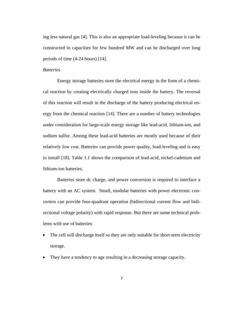
Batteries

Energy storage batteries store the electrical energy in the form of a chemi-

cal reaction by creating electrically charged ions inside the battery. The reversal

of this reaction will result in the discharge of the battery producing electrical en-

ergy from the chemical reaction [14]. There are a number of battery technologies

under consideration for large-scale energy storage like lead-acid, lithium-ion, and

sodium sulfur. Among these lead-acid batteries are mostly used because of their

relatively low cost. Batteries can provide power quality, load-leveling and is easy

to install [18]. Table 1.1 shows the comparison of lead-acid, nickel-cadmium and

lithium-ion batteries.

Batteries store dc charge, and power conversion is required to interface a

battery with an AC system. Small, modular batteries with power electronic con-

verters can provide four-quadrant operation (bidirectional current flow and bidi-

rectional voltage polarity) with rapid response. But there are some technical prob-

lems with use of batteries:

The cell will discharge itself so they are only suitable for short-term electricity

storage.

They have a tendency to age resulting in a decreasing storage capacity.

8

Table 1.1. Specification of batteries

Battery type

Specification

Lead acid Nickel cadmium Lithium-ion

Energy density (Wh-kg) 30-50 45-80 150-190

Cell voltage

(V)

2 1.2 3.6

Overcharge tolerance High Moderate Low

Cycle life

(80% discharge)

200-300 1000 500-1000

Charge time (h) 8-16 1 2-4

Toxicity Very high Very high Low

Cost ($/Wh) 0.125-0.2 0.4-0.8 0.2-0.36

*Sources of data: [16]-[18]

Thermal energy storage

Thermal energy storage (TES) can be divided in two different types. First-

ly, TES applicable to solar thermal power plants and secondly its end-use [20].

TES for a solar thermal power plant consists of a synthetic oil or molten salt that

stores solar energy in the form of heat collected by solar thermal power plants to

enable smooth power output during daytime cloudy periods and to extend power

production for 1-10 hours past sunset [21]. End-use TES stores electricity from

off-peak periods through the use of hot or cold storage in underground aquifers,

water or ice tanks, or other storage materials and uses this stored energy to reduce

the electricity consumption of building heating or air conditioning systems during

times of peak demand [22]. During off-peak periods ice can be made from water

using electricity, and the ice can be stored until next day when it is used to cool

9

either the air in a large building, thereby shifting the demand off-peak. Using

thermal storage can reduce the size and initial cost of cooling systems, lower en-

ergy costs and maintenance costs.

Hydrogen

Hydrogen storage involves using electricity to split water into hydrogen

and oxygen through a process called electrolysis. Compressed hydrogen is the

simplest system to conceive. When electricity is needed the hydrogen can be used

to generate electricity through a hydrogen powered combustion engine or a fuel

cell. Hydrogen fuel cells can be used in power quality applications where 15 se-

conds or more of ride-through are required. On a life-cycle cost basis for long du-

ration applications, fuel cell technology competes with battery systems at dis-

charge times greater than about 2 hours, depending on cost assumptions, and with

hydrogen-fueled engines at discharge times greater than about 4 hours. Typical

energy efficiency of a fuel cell is between 40-60%, or up to 85% efficient if waste

heat is captured for use [23]-[24].

Flywheels

A flywheel is an electromechanical storage system in which energy is

stored in the form of kinetic energy of rotating mass. The charging or discharging

of the flywheel storage system takes place by changing the amount of kinetic en-

ergy present in the accelerating or decelerating rotor, respectively [4]. The fly-

wheel is coupled with an electrical machine which acts as a motor to drive the

10

flywheel while charging and acts as a generator to discharge the stored energy by

decelerating the rotor to stationary position. During charging, an electric current

flows through the motor increasing the speed of the flywheel. During discharge,

the generator produces current flow out of the system slowing the wheel down

[25].

Ultra capacitors / super capacitor

Capacitors store their energy in an electrostatic field rather than in chemi-

cal form. These consist of two parallel electrode plates which are separated by a

dielectric. When the voltage is applied across the terminals the positive and nega-

tive charges get accumulated over the electrodes of opposite polarity. The capaci-

tor stores energy by increasing the electric charge accumulation on the metal

plates and discharges energy when the electric charges are released by the metal

plates. Ultra-capacitors are now available in the range of up to 100 kW with very

a short discharge time of up to ten seconds [26]. Ultra-capacitors have tempera-

ture independent response, low maintenance and long lifetimes, but they have rel-

atively high cost. These devices also have high loss and they are intended to be

operated only for a few seconds.

Super Conducting Magnetic Energy Storage (SMES)

Superconducting magnetic energy storage is an energy storage device that

stores electrical energy in magnetic field without conversion to chemical or me-

11

chanical form. In SMES, a coil of superconducting material allows DC current to

flow through it with virtually no loss at very low temperatures. This current cre-

ates the magnetic field that stores the energy. On discharge, switches tap the cir-

culating current and release to serve the load with high power output in short in-

terval of time [25]. Although the SMES device itself is highly efficient and has no

moving parts, it must be refrigerated to maintain superconducting properties of

the wire materials. Therefore, SMES devices require cryogenic refrigerators and

related subsystems, thus increasing maintenance costs [14].

Table 1.2 summarizes some of these storage technologies and their charac-

teristics.

1.5 Organization of this thesis

This thesis is organized into five chapters. Chapter 2 presents basic con-

cepts of optimal dispatch including different economic dispatch methodologies.

These concepts are used in the formation and solution of the algorithm for optimal

energy storage.

Chapter 3 demonstrates the idea of optimal scheduling of energy storage

using a small illustrative example. Chapter 4 illustrates application of this algo-

rithm in the state of Arizona as a test bed. The test bed is a subset (equivalent) of

the Western Electricity Coordinating Council system.

12

Chapter 5 presents conclusions, contributions from the test beds studied

in Chapter 4 and lines of future work regarding the use of large scale energy stor-

age in power systems.

There are two appendices provided. Appendix A shows the corresponding

Matlab algorithm for the DC optimal power flow developed during this research.

Appendix B describes the quadratic programming algorithm.

13

Lif

etim

e

(yea

rs)

40

30

2-1

0

40

10

20

20

40

40

Res

po

nse

tim

e

(ms)

30

30

00

-

15

00

0

30

5 5

5

Po

wer

lev

el

(MW

)

<2

000

10

0-3

00

<3

0

26

0

< 0

.10

0

(eac

h)

0.2

00

0.1

00

Dis

char

ge

tim

e

12

hou

rs

4-2

4 h

ou

rs

1-8

ho

urs

6 h

ours

min

to 1

h

10

s

10

s

Mat

uri

ty

Co

mm

erci

al

Co

mm

erci

al

Co

mm

erci

al

Co

mm

erci

al

Co

mm

erci

al

Co

mm

erci

al

Rec

ent

com

mer

cial

Co

mm

erci

al

Co

mm

erci

al

Mai

nte

-

nan

ce c

ost

($/M

Wh

)

4

3

15

10

3

4

5

1

Eff

icie

ncy

0.8

0.8

5

0.7

-0.8

5

0.8

0.4

5-0

.8

0.9

0.9

3

0.9

5

0.9

7

Wei

gh

t

(kg

/MW

h)

3,0

00

2.5

30

0,0

00

30

7,5

00

3,0

00

10

,000

10

Cap

ital

co

st

($/

MW

h)

7,0

00

2,0

00

550

15,0

00

300,0

00

25,0

00,0

00

28,0

00,0

00

10,0

00

*S

ou

rces

of

dat

a [1

2]-

[26]

Cap

acit

y

22,0

00

MW

h

2,4

00

MW

h

200 M

Wh

400 M

Wh

0.3

-2000

kW

h

50 k

Wh

750 k

Wh

0.5

kW

h

0.8

kW

h

Sto

rage

met

hod

Pu

mp

ed

Hy

dro

CA

ES

Bat

teri

es

Th

erm

al

ener

gy

Hy

dro

-

gen

Fly

whee

l

(low

spee

d)

Fly

whee

l

(hig

h

spee

d)

Ult

ra c

a-

pac

ito

r

SM

ES

Tab

le 1

.2 A

com

par

ison o

f bulk

ener

gy s

tora

ge

tech

nolo

gie

s

14

Chapter 2. Optimal Dispatch of Energy Storage Systems

2.1. Power system operation

The operation of power systems involves the best utilization of the availa-

ble energy resources. The operation generally subjected to various constraints to

transfer electrical energy from generating stations to the consumers with maxi-

mum safety without interruption of supply.

Prior to restructuring of the power system in the U.S., unit commitment

(identifying the generators which when dispatched, will give the available least-

cost operation of available generation resources to meet the electrical load) [32]

and economic dispatch were performed by vertically integrated utilities. This op-

erating strategy is done to minimize the production cost of generation. Occasion-

ally, there are power exchanges or interchanges between utilities to take economi-

cal advantage of power interchanges. Power pools were formed by several inter-

connected utilities to effectuate this exchange. Traditionally, coordinating unit

commitment and economic dispatch were performed by a central dispatch office

[31].

There are three stages in system control, namely unit commitment, securi-

ty analysis and economic dispatch [36]:

Unit commitment involves the hour-by-hour ordering of generator units start-

up/shut-down in the system to match the anticipated load.

15

With a given power system topology and a given number of generators, secu-

rity analysis assesses the system response to a set of contingencies and pro-

vides a set of constraints that should not be violated if the system is to remain

in secure state.

Economic dispatch orders the minute-to-minute loading of the connected

generating plants so that the cost of generation is minimum subject to con-

straints. Figure 2.1 illustrates the operation and data flow in a modern power

system.

Load forecastingUnit commitment Security analysis

Data base

State estimation

Power system

Economic dispatch

Figure 2.1 Power system control activities

2.2. The theory of optimal dispatch

The definition of optimal or economic dispatch provided in EPAct section

1234 is “The operation of generation facilities to produce energy at the lowest

cost to reliably serve consumers, recognizing any operational limits of generation

and transmission facilities” [27].

16

The fuel cost ($/h) of a thermal unit is often expressed as an approximate-

ly quadratic function of the power output (MW) of the unit. Therefore the incre-

mental cost ($/MWh) is almost linear with respect to the unit power output. With-

out considering other parameters (e.g., transmission losses, reactive losses, line

constraints, unit output power constraints), the most economical generation levels

occur when the incremental costs of all available units are equal. This simple rule

is known as the ‘equal incremental cost rule’ and this is a result of elementary

analysis and formulation of the problem as a Lagrange multiplier optimization

[28]. If a unit has a higher incremental cost at an output level than other units, it

would be cheaper to generate the MW from another unit with a lower incremental

cost. The ‘equal incremental cost rule’ needs to be modified when the generator

output limits and the transmission losses are taken into consideration. When the

MW output level of a unit reaches its upper limit, the unit output is fixed at the

upper limit even if the system load increases. Other units which have not reached

their maximum limits would share the load increase bases on the ‘equal incremen-

tal cost’ rule. To account for the transmission losses, the incremental costs are

modified with a ‘penalty factor’. The penalty factor is a measure of additional

transmission losses due to an incremental increase in the unit output [31].

There are many conventional methods that are used to solve the economic

dispatch problem such as the Lagrange multiplier method, lambda iteration. These

methods need to compute the economic dispatch each time load changes. As a

result, long computation times may result.

17

2.3. Economic dispatch methodologies

There are various techniques including traditional and modern optimiza-

tion methods developed for the economic dispatch without security-constrained

(i.e. operation of the power system under credible contingencies). These methods

can be classified as conventional optimization methods and intelligent search

methods [33]. The conventional optimization methods include lambda-iteration,

linear programming (LP), quadratic programming (QP), dynamic programming,

and mixed integer programming. Among these methods lambda-iteration method

is simple, more favorable, and used in many commercial economic dispatch pro-

grams. Some of the intelligence search methods are neural network and particle

swarm optimization (PSO).

The system incremental fuel cost rate, called system lambda, is the key to

find the most economical generation output of all on-line units. However, when

the cost function is more complex than a piecewise linear function or a quadratic

function, other methods are more suitable than the lambda-iteration method [31].

The conventional optimization methods are discussed below in brief:

The lambda-iteration method:

In lambda iteration method, lambda is the variable introduced in solving

constraint optimization problem and is called Lagrange multiplier. All the ine-

quality constraints to be satisfied in each trial, the equations are solved by the it-

erative method [31]:

18

Step 1. Assume a suitable value of λ(0)

this value should be more than the largest

intercept of the incremental cost characteristic of the various generators.

Step 2. Compute the individual generations i.e. calculate Pgi for i = 1,2…,N.

Step 3. First iteration, check the equality constraint i.e. tolerance, ϵ = PL - ∑ Pgi

for i = 1,2…,N. If not satisfied set a new value of λ and repeat the above steps.

Step 4. Check the convergence. If ΔPgi in step 3 are below the user-defined toler-

ance, the solution converges. Otherwise, go to step 2.

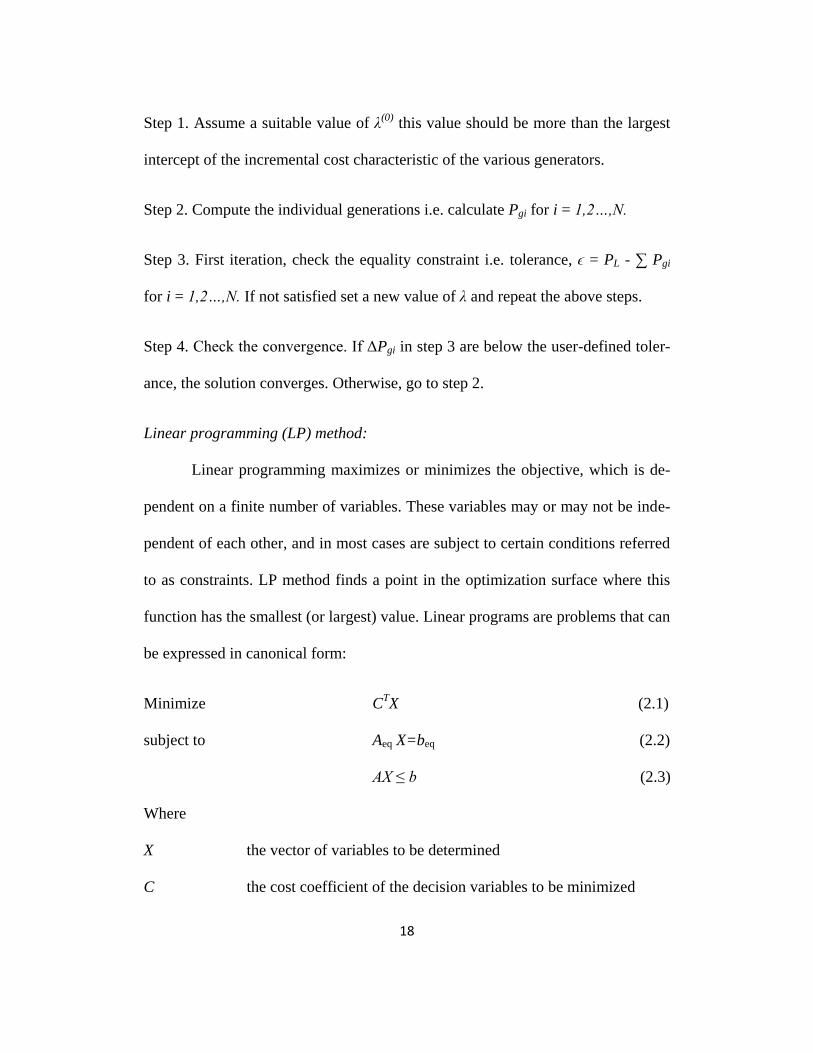
Linear programming (LP) method:

Linear programming maximizes or minimizes the objective, which is de-

pendent on a finite number of variables. These variables may or may not be inde-

pendent of each other, and in most cases are subject to certain conditions referred

to as constraints. LP method finds a point in the optimization surface where this

function has the smallest (or largest) value. Linear programs are problems that can

be expressed in canonical form:

Minimize CTX (2.1)

subject to Aeq X=beq (2.2)

AX ≤ b (2.3)

Where

X the vector of variables to be determined

C the cost coefficient of the decision variables to be minimized

19

A, Aeq an (m x n) constraint matrix

B, beq an m-dimensional column vector of right hand side constraints

The method for solving economic dispatch by LP uses an iterative technique to

obtain the optimal solution [33]:

Step 1. Select the set of initial control variables.

Step 2. Solve the power flow problem to obtain a feasible solution that satisfies

the power balance equality constraint.

Step 3. Linearize the objective function and inequality constraints around the

power flow solution and formulate the LP problem.

Step 4. Solve the LP problem and obtain optimal incremental control variables

ΔPgi.

Step 5. Update and form the new control variables Pgi new=Pgi old + ΔPgi.

Step 6. Obtain the power flow solution with updated control variables.

Step 7. Check the convergence. If ΔPgi in step 4 are below the user-defined toler-

ance, the solution converges. Otherwise, go to step 3.

Quadratic programming method:

Quadratic programming is a special form of nonlinear programming

whose objective function is quadratic and constraints are linear. The most often

used objective function in power system optimization is the generator cost func-

20

tion, which generally is a quadratic. The linear programming method can also be

used in the quadratic programming model of economic dispatch (see Appendix

B).

Dynamic programming (DP) method:

The basic idea of the theory of DP is that of viewing an optimal policy as

one determining the decision required at each time in terms of the current state of

the system. This absolute problem is normally solved by discretization of the en-

tire dispatch period into a number of small time intervals over which the load is

assumed to be constant and the system is considered to be in steady-state [37].

There are two DP algorithms. They are forward and backward dynamic program-

ming. The start-up cost of a unit is a function of the time. The forward approach is

often adopted since the initial condition is known. The backward DP algorithm is

appropriate when the terminal condition is known. Suppose a system has n units.

There is 2n – 1 combination.

The recursive algorithm is used to compute the minimum cost in hour k

with state n is [31],

Fcos t (k,n)= min[Pcos t (k,n) + Scos t (k –1, m:k,n) + Fcos t (k –1,m)] (2.4)

where

Fcos t (k,n) The total cost from initial state to hour k state n

Scos t (k –1, m:k,n) The transition cost from state (k –1, m) to state (k,n)

m The set of states at hour t – 1

21

Pcos t (k,n) The production cost for state (k,n)

This thesis uses the process of applying the quadratic programming meth-

od to a minimization problem. The QP method is a very powerful solution algo-

rithm because of their rapid convergence near the solution. This property is espe-

cially useful for the power system application because an initial guess near the

solution is easily attained.

2.4. Formulation of the optimal bulk storage problem

A general minimization problem can be written in the following form:

Minimize f(X) (the objective function) (2.5)

subject to: hi(X )= 0 i = 1,2…,m (equality constraints) (2.6)

gj(X) ≤ 0 j = 1,2…,n (inequality constraints) (2.7)

There are m equality constraints and n inequality constraints and the num-

ber of variables is equal to the dimension of the vector X. The system described

has constraints that capture line ratings, generator ratings, bus power conservation

and the Kirchhoff laws.

The mathematical model of real power economic dispatch with security

constraints can be written as follows:

Minimize f(X) =

ci Pgi + Pgi T

Q Pgi i ϵ ng (2.8)

subject to AeqX = beq (2.9)

AX ≤ B (2.10)

22

such that ∑Pgi=∑PLk i ϵ ng; k ϵ nl

Pij min ≤ Pij ≤ Pij max ij ϵ nt

0 ≤ Pgi ≤ Pgi max i ϵ ng

Psq min ≤ Ps ≤ Psq max q ϵ ns

0 ≤ Es ≤ Esq max q ϵ ns

Where

PL The real power load in MW

Pij The power flow of transmission line ij in MW

Pij min , Pij max The minimal and maximal power limits of transmission line ij in MW

Pgi The real power output at generator bus i in MW

Pgi min, Pgi max The minimal and maximal real power output at generator i in MW

Psq min, Psq max The minimal and maximal storage capacity at storage i in MW

Esq max The maximal energy storage at storage i MWh

ci The cost of the generator i

nl The number of transmission lines

ng The number of generators

ns The number of large scale storage system

Q (n x n) symmetric matrix describing the coefficients of quadratic terms

X The n-dimensional column vector of decision variables (note: X con-

tains: (1) control variables such as generation and storage power levels

as well as (2) problem unknowns such as line flows and bus voltage

phase angles)

23

Problem of dimensionality

Generally, the number of unknowns X increases like (nb+ ns + nl+ nb- 1)h.

The number of equality constraints increases like (nb+ nb)h + 1.

The number of inequality constraints increases like (2nl+ ns)h + ns( 2h-2).

where

Equality constraints

The equality constraints (Aeq) of the optimal power flow (OPF) reflect the

physics of the power system. The following equality constraints are enforced dur-

ing QP.

Conservation of power at each bus: The physics of the power system are en-

forced through the power flow equations which require that the net injection

of real power at each bus sum to zero. The corresponding generation limits of

individual generator are accommodated in the upper bound (UB) and lower

bound (LB) of the programming.

Line load versus phase angle at each bus: Assumption is the voltage at the

nodes is 1 p.u.

Pij = (δi – δj)/ (xij).

Charge /discharge schedule for all the storage elements should sum up to zero.

∑Psi=0 i ϵ ns.

nb The number of buses in the system.

h The number of interval of hours of a day.

24

Inequality constraints

In addition to the equality constraints, there are inequality constraints (A)

in the model. The inequality constraints in the OPF reflect the limits on physical

devices in the power system as well as the limits created to ensure system securi-

ty. Physical devices that require enforcement of limits are:

Line loads

Conservation of energy (storage)

Power to storage element.

25

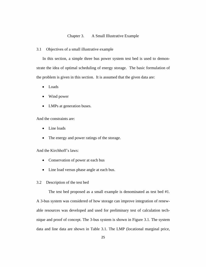
Chapter 3. A Small Illustrative Example

3.1 Objectives of a small illustrative example

In this section, a simple three bus power system test bed is used to demon-

strate the idea of optimal scheduling of energy storage. The basic formulation of

the problem is given in this section. It is assumed that the given data are:

Loads

Wind power

LMPs at generation buses.

And the constraints are:

Line loads

The energy and power ratings of the storage.

And the Kirchhoff’s laws:

Conservation of power at each bus

Line load versus phase angle at each bus.

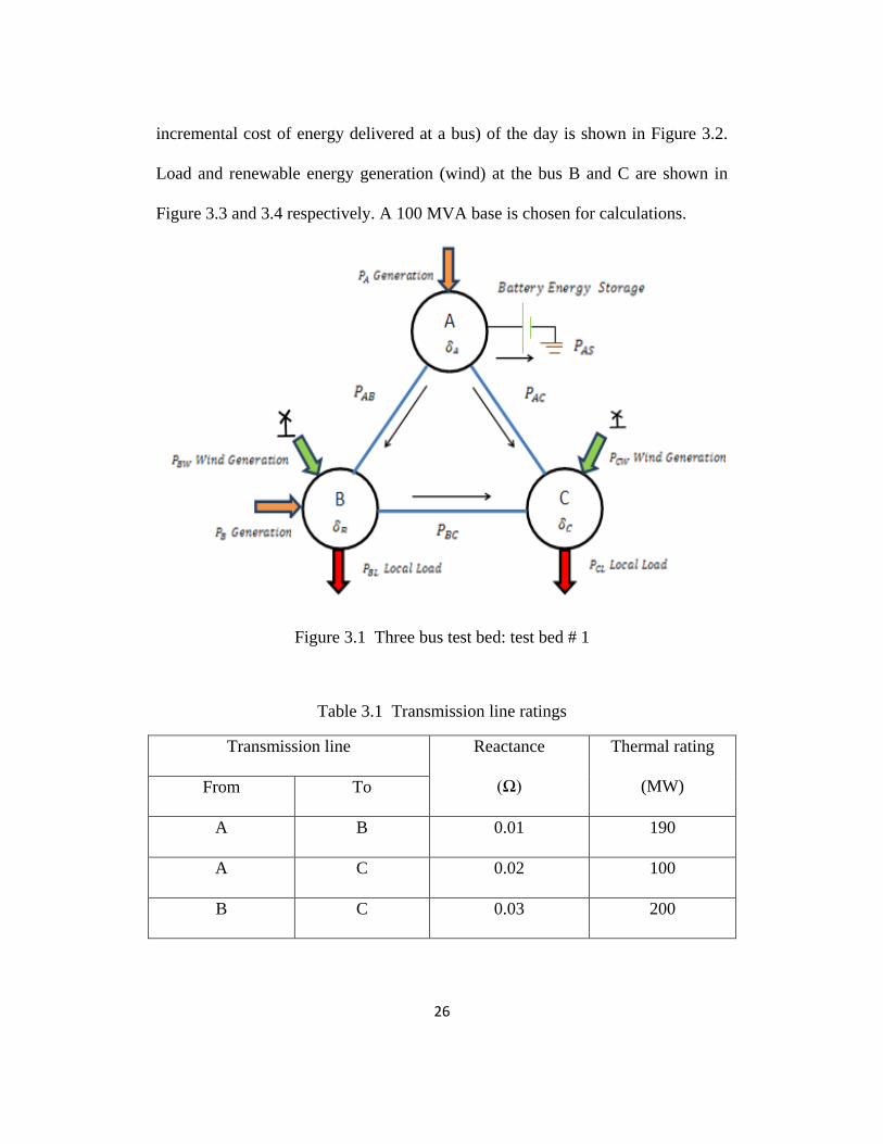
3.2 Description of the test bed

The test bed proposed as a small example is denominated as test bed #1.

A 3-bus system was considered of how storage can improve integration of renew-

able resources was developed and used for preliminary test of calculation tech-

nique and proof of concept. The 3-bus system is shown in Figure 3.1. The system

data and line data are shown in Table 3.1. The LMP (locational marginal price,

26

incremental cost of energy delivered at a bus) of the day is shown in Figure 3.2.

Load and renewable energy generation (wind) at the bus B and C are shown in

Figure 3.3 and 3.4 respectively. A 100 MVA base is chosen for calculations.

Figure 3.1 Three bus test bed: test bed # 1

Table 3.1 Transmission line ratings

Transmission line Reactance

(Ω)

Thermal rating

(MW) From To

A B 0.01 190

A C 0.02 100

B C 0.03 200

27

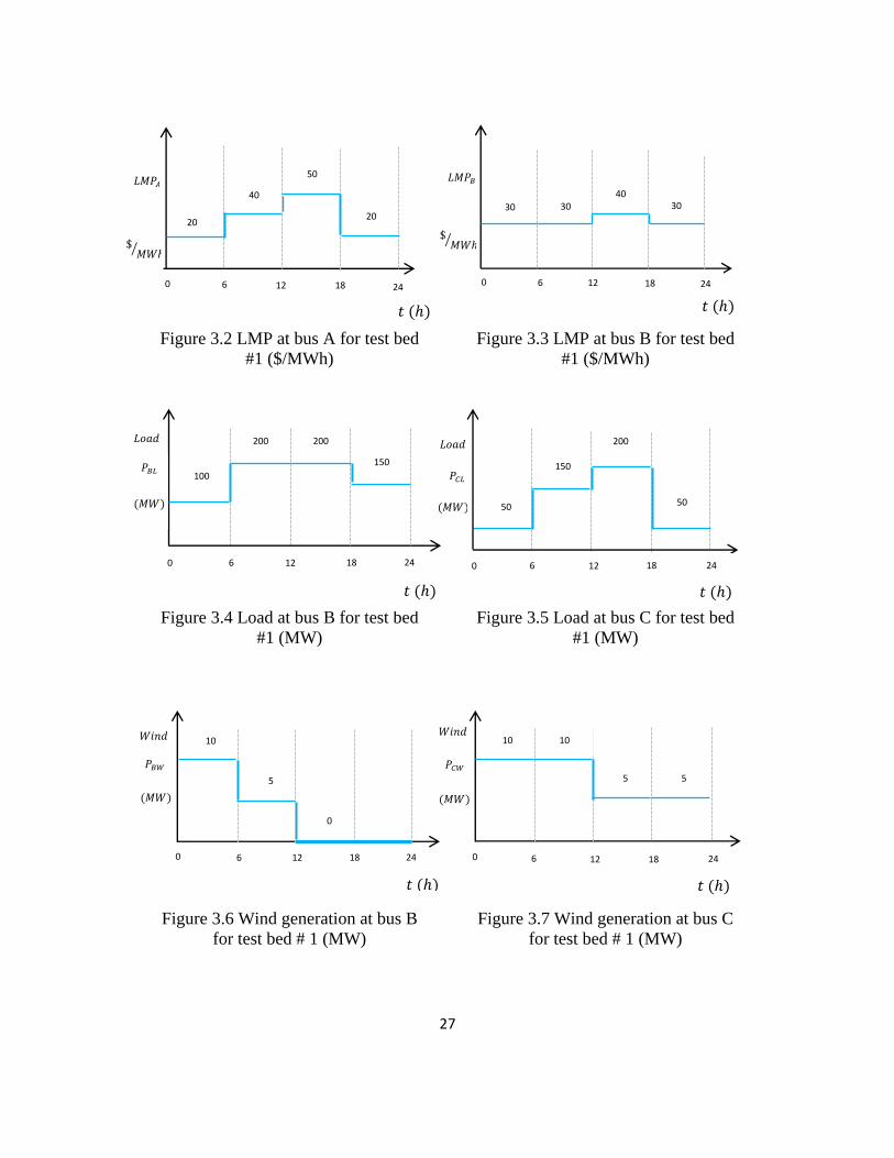
Figure 3.2 LMP at bus A for test bed

#1 ($/MWh)

Figure 3.3 LMP at bus B for test bed

#1 ($/MWh)

Figure 3.4 Load at bus B for test bed

#1 (MW)

Figure 3.5 Load at bus C for test bed

#1 (MW)

Figure 3.6 Wind generation at bus B

for test bed # 1 (MW)

Figure 3.7 Wind generation at bus C

for test bed # 1 (MW)

20

$𝑀𝑊ℎ

0 6 12 18 24

𝑡 (ℎ)

20

40

50 𝐿𝑀𝑃𝐴

$𝑀𝑊ℎ

6 18 24 12 0

𝑡 (ℎ)

30 30 30 40

𝐿𝑀𝑃𝐵

𝐿𝑜𝑎𝑑

𝑃𝐵𝐿

(𝑀𝑊)

100

6 12 0

200

24 18

𝑡 (ℎ)

200

150

200

50 (𝑀𝑊)

𝐿𝑜𝑎𝑑

𝑃𝐶𝐿

50

150

𝑡 (ℎ)

24 0 6 12 18

𝑊𝑖𝑛𝑑

(𝑀𝑊)

𝑃𝐵𝑊

0 6 12 18 24

𝑡 (ℎ)

10

5

0

𝑊𝑖𝑛𝑑

𝑃𝐶𝑊

(𝑀𝑊)

10 10

5 5

𝑡 (ℎ)

0 6 24 18 12

28

3.3 Formulation of the problem

The main objective is to maximize beneficial impacts of storage, mainly

reflected as minimizing generation dispatch cost. A storage facility is considered

to be present at Bus A in Figure 3.1. A QP based algorithm is carried out to opti-

mize generation and storage scheduling with maximal use of renewable genera-

tion. For the tests reported, all the wind generation is used. The unknowns, opti-

mum generation schedule and storage (store/discharge) schedule are calculated,

minimizing the purchase price of energy for one day. The information used and

constraints considered are mentioned below:

Given Information

Loads

Wind power

LMPs at generation buses

Constraints

Line loads

Energy and power of storage

Conservation of power at each bus

Voltage phase angle at each bus

Bus A is assumed to be the reference bus. The voltage phase angle at each

bus constrained to lie between -30o ≤ δ ≤ 30

o. Three cases are studied calculating

the economic dispatch of generation at bus A (PA) and bus B (PB) for minimum

cost with:

No storage and no constraints line ratings.

Constraint on line ratings and one storage unit at bus A.

Constraint on line ratings and two storage units at bus A and B.

29

All the three cases are studied for a one day time horizon broken into 4 intervals

each have a span of 6 hours.

3.4 Study of case 1 (base case)

In this case study, the system is initially assumed without energy storage

and without constraints on line ratings are considered. After executing the eco-

nomic dispatch considering the limits on generation, the output of generating units

PA and PB computed is listed in Table 3.2. The minimum generation cost of the

system without energy storage using QP in Matlab is 181,520 dollars per day. At

interval 1 and 4, the load is being supplied by the cheap unit A. At intervals 2 and

3, the cheap unit B has to supply power.

Table 3.2 Case 1 study results, test bed #1

Interval (each

Operational data 6 hours) 1 2 3 4

Generation

(MW)

Bus A 130 0 0 195

Bus B 0 335 395 0

Line flows

(MW)

Bus A to Bus B 88.33 -70 -97.5 140

Bus A to Bus C 41.67 70 97.5 55

Bus B to Bus C -1.67 70 97.5 -100

Voltage an-

gle (radians)

Bus B -0.0088 0.007 0.0097 -0.014

Bus C -0.0083 -0.014 -0.0195 -0.011

30

3.5 Study of case 2

In this case study, with the energy storage at bus A having rating of 20

MW and energy capacity of 120 MWh. Economic dispatch of generations PA and

PB is calculated for minimum cost using QP in Matlab with storage and consider-

ing the limits on generations and thermal ratings of the transmission lines. The

dispatch results are shown in Table 3.3. At the first low-load hour, the storage is

charged by 20 MW which is from the cheap unit A. At intervals 2 and 3, the out-

put from the storage is discharged mitigating the congestion on the line from bus

A to bus C. In addition the output from the battery is replacing generation from

expensive unit A. The total generation dispatch cost is 179,380 dollars per day

which is less than that in case 1. This saving could be much higher in the large

system.

From case 2 it is observed, the energy is stored during the minimum cost

of generation and discharged when the cost of generation is high. At the end of

the day the storage element is completely discharged. In other words the battery

(storage element) charges during the first interval and discharges during the se-

cond and third interval to minimize the cost of generation

31

Table 3.3 Case 2 study results, test bed #1

Interval (each

Operational data 6 hours) 1 2 3 4

Generation (MW)

Bus A 150 0 0 195

Bus B 0 330 380 0

Line flows (MW)

Bus A to Bus

B 88.33 -65.83 -85 140

Bus A to Bus

C 41.67 70.83 100 55

Bus B to Bus C -1.67 69.17 95 -100

Voltage angle

(radians)

Bus B -0.0088 0.0066 0.0085 -0.014

Bus C -0.0083 -0.0142 -0.02 -0.011

Storage (MW) Bus A 20 -5 -15 0

3.6 Study of case 3

In case 3 the economic dispatch is solved with limits on line ratings and

two storage units at bus A and bus B having combined rating of 20 MW and ener-

gy capacity of 120 MWh (10 MW and 60 MWh each). The results are shown in

Table 3.4. The cost of economic dispatch of generation per day calculated is $

179,080.

32

Figure 3.8 Three bus test bed: test bed # 1 with two storage units

Inference drawn from this case is that the spreading the storage unit reduc-

es the generation production cost. This is because of line rating constraints limit-

ing concentrated energy storage. At the first low-load hour, the storage at bus A

and bus B is charged by 10 MW each which is from the cheap unit A. At interval

4, the output from the storage is discharged mitigating the congestion on the line.

In addition the output from the battery is replacing generation from expensive unit

A and B. The total generation dispatch cost is 179,080 dollars per day which is

less than that in case 2.

33

Table 3.4 Case 3 study results, test bed #1

Interval (each

Operational data 6 hours) 1 2 3 4

Generation

(MW)

Bus A 150 0 0 195

Bus B 0 335 375 0

Line flows

(MW)

Bus A to Bus B 96.67 -70 -89.7 140

Bus A to Bus C 43.33 70 99.17 55

Bus B to Bus C -3.33 70 95.83 -100

Voltage angle

(radians)

Bus B -0.0097 0.0070 0.0089 -0.014

Bus C -0.0087 -0.014 -0.0198 -0.011

Storage (MW)

Bus A 10 0 -10 0

Bus B 10 0 -10 0

3.7 Impact of storage: observations from test bed # 1

The implementation and use of renewable energy may not always be pos-

sible due to constraints of transmission and component ratings, when storage is

34

added; these constraints are partially relaxed, this can be observed from cases

mentioned above.

High prices are one of the largest barriers facing renewables. During peak

demand on the electric grid, electric companies pay more for electricity. Often

additional power needs at this time are supplied by natural gas or oil, which has

higher fuel costs. The opposite is true during times of low demand, when elec-

tricity costs are lower, during this time the energy can be stored and discharged

when the demand and fuel cost is high thereby reducing the overall cost of gen-

eration per day; this can be observed from the above discussed cases 1, 2 and 3.

The grid needs a consistent, stable supply of energy that can be adjusted

during times of peak demand. Black out occurs when supply does not keep up

with demand. High demand on the power grid often requires power plants to be

fired up to cover short-term electricity demand at a higher price. Large-scale of

use of renewable energy will require that it can adapt to variable levels of demand

on the power grid. Energy storage combined with these renewable energy re-

sources may firm up the power output.

The cost of delivery and generation (fuel) can be minimized by increasing

the capacity of storage elements and fuel cost can be further optimized by disburs-

ing the storage unit across the power system. This concept is illustrated in Figure

3.9. Here, corresponding to the total power (MW, across two storage units), six

hours of energy storage (MWh) is considered.

35

Figure 3.9 Fuel cost comparison with one and two storage unit

Energy storage gives additional degrees of freedom in the optimal dispatch

problem, thereby potentially allowing the additional use of renewable energy. The

simple example of test bed #1 shown has wind penetration in the range of 5 %

(Wind peak power / Peak demand power). Much more significant improvements

in operating strategies occur at higher storage capacities. This is shown in the Ta-

ble 3.5.

36

Table 3.5 Cost comparison with one and two storage units.

Total Storage Capacity

(MW)

Fuel cost per day to serve the load ($/day)

One storage unit Two storage unit

0 181,520 181,520

10 180,320 180,320

20 179,380 179,080

30 178,810 177,910

40 178,210 177,010

50 177,610 176,110

60 177,010 175,210

70 176,410 174,310

80 175,810 173,410

90 175,210 172,510

100 174,610 171,610

110 174,010 170,710

120 173,400 169,810

37

Chapter 4. Illustrative Example using the State of Arizona as a Test Bed

4.1 Description of the test bed: State of Arizona

The previous chapter provided an introduction test system to demonstrate

the idea of optimal scheduling of energy storage. This chapter looks at more real-

istic and well-studied example. In this section, the effect of energy storage on the

minimization of the objective function using the State of Arizona as a test bed

with different storage capacities and wind generation is studied. This benchmark

system which represents a portion of the Western Electricity Coordinating Coun-

cil (WECC) as of April 2009 does not include storage. Therefore, while the use of

its network topology, generation bounds as well as transmission line ratings

bounds, appropriate values for the storage parameters are added in the profile. The

load, wind power and LMPs (assumed, at generation bus) at each bus are also

given. The heavy summer case of 2009 is considered (actual load and generation

data).

In the test case, an objective function is minimized. Again, this corre-

sponds to minimum operating cost. The constraints and formulation of the prob-

lem is the same as provided in the previous chapter. A QP based algorithm is car-

ried out to optimize generation and storage scheduling with maximal use of re-

newable generation. The optimum generation schedule, storage (store / discharge)

schedule, and line flows are control variables, and these quantities are calculated.

38

A one day time horizon broken into 3 intervals each having a span of 8

hours is studied. The objective of the constrained economic dispatch is to sched-

ule the generation outputs economically including storage over one day. The

simplifications made are:

Reactive power flows are not modeled or considered

A simple linear relationship is assumed between bus voltage phase angle

and line active power flows

Transmission line losses are neglected.

The portion of the WECC under study is mainly the state of Arizona having the

description profile indicated in Table 4.1.

Table 4.1 Description profile: state of Arizona power system

Number of buses nb 792 Number of generators 182

Number of lines nl 1079 Number of wind farms * 2

*Assumed

4.2 Case 4

Case 4 is a ‘base case’ study for this test bed. In case 4, no storage units

are scheduled and two wind farms are located at Flagstaff and Springerville. Eco-

nomic dispatch of generations is calculated for the minimum cost using QP in the

Matlab optimization toolbox. According to the constraints considered in this

work, only active power constraints are considered. Therefore, the respective

39

maximum and minimum operating long term thermal ratings of the transmission

lines, generation limits and voltage phase angle limits at each bus is accommodat-

ed in the upper (UB) and lower bound (LB) of the program.

Table 4.2 shows the operational data for case 4. The cost of economic dis-

patch of generation per day calculated is 12.049 million dollars per day (M$/day).

Table 4.2 Case 4 study results, Arizona test bed

Wind Storage

P1 (MW) P2 (MW) P1 (MW) W1(MWh) P2 (MW) W2 (MWh)

400 300 0 0 0 0

4.3 Case 5 – storage added

In case 5, the wind power capacity and storage capacity is increased. The

case is divided under low, medium and high depending on wind power penetra-

tion and storage capacity of the power system. Two wind farms are considered

located at Flagstaff and Springerville along with two storage units both at Navajo.

The storage units have two ratings, one relating to the power electronic converters

(this is the power rating of the unit), and the other as the ultimate energy storage

capability (this is the energy rating, e.g., in MWh). For case 5, it is assumed that

the power rating (MW) times 6 hours is the energy (MWh) rating.

Table 4.3 tabulates the description of the wind power and storage as well as

the solution cost. It is observed that with increasing energy storage, the operating

40

cost reduces. Note that electrical energy is stored during times when generation

cost is low and when production exceeds consumption. The stored energy is dis-

charged during the period when the production cost from conventional generating

plants is high.

Table 4.3 Case 5 study results, Arizona test bed

Scenario

Operational data

Low

1

Medium

2

High

3

Win

d

P1 (MW) 400 600 800

P2 (MW) 300 500 600

Sto

rage

P1 (MW) 50 100 300

P2 (MW) 50 150 250

W1 (MWh) 300 600 1800

W2 (MWh) 300 900 1500

Cost

QP (Million

dollars / day) 11.772 11.453 11.066

4.4 Case 6 – increase in the number of storage units

In case 6, three scenarios are studied. The number of energy storage units is

increased from 2 to 4 to 6. In each scenario, the total power and energy stored is

41

the same, i.e. total power capacity = PST = 700 MW and total energy WST = 4200

MWh. These levels are shared among the storage units. The wind power is the

same as assumed in case 4. Table 4.4 tabulates the number of storage units and

economic dispatch cost in millions of dollars per day obtained using QP for the

respective scenarios.

The results indicate that the cost of delivery and generation (fuel) can be

minimized by increasing the capacity of storage elements. The fuel cost can be

further optimized by selecting optimum locations for the two storage units.

Table 4.4 Case 6 study results, Arizona test bed

Scenario

Operational Data

1 2 3

Sto

rage

Number of Units 2 4 6

P (MW)

each unit 350 175 116.67

W (MW)

each unit 2100 1050 700

Cost

QP (M$/day) 11.616 11.563 11.484

4.5 Case 7 – large scale implementation

This case resembles more of a practical scenario. In other words, a large

number of wind machines are accommodated. Note that the 2025 renewable port-

42

folio standard for Arizona is 15%; a higher percentage of wind generation is ac-

commodated in case 7. In case 7, 15% of the total load is derived from wind gen-

eration. Also, ten energy storage units are represented having a total capacity of

700 MW with 6 hours of energy storage (i.e., the total energy rating is 6 times 700

or 4200 MWh). Table 4.5 shows the system description.

Table 4.5 Case 7 system description

Number of buses nb 792 Number of lines nl 1079

The wind availability considered throughout the day for case 7, and this is

shown in Fig. 4.1. The wind turbines are assumed to generate power at name plate

rated capacity. The cost of economic dispatch of generation computed is 10.863

million dollars per day (M$/day).

The inference made from this case is the optimal location of energy stor-

age units is at the generation buses. This observation is made for storage units

such as batteries; however, obviously, the location of pumped-hydro storage is

dictated by geography and topography. Storage units can be placed next to wind

farms to produce a consistent flow of power. Locations like Bullhead City have a

high potential of wind production [5]. Siting wind generation at such locations

may be dependent on ratings of the adjacent transmission facilities. Storage unit

placed at these locations can store excess wind energy and discharge during later

43

periods. Therefore, use of storage can reduce the cost of upgrade of the electricity

link and defer the expansion of the transmission network.

Figure 4.1 Wind generation patterns for case 7, t is in hours

4.6 Calculation of payback period

The payback period in capital budgeting refers to the period of time re-

quired to return an investment, to repay the sum of the original investment. An

approximate payback period is calculated for the above discussed cases 5, 6 and

7. Mathematically, the length of time required to recover the cost of an invest-

ment is calculated as:

= Cost of Project / Annual Cash Inflows

44

There are two main problems, with the payback period method:

It ignores any benefits that occur after the payback period and, therefore,

does not measure profitability.

It ignores the time value of money.

Annual cash inflows is the savings obtained from cases 5, 6, and 7 when

compared with case 4. Following assumption is made:

The energy storage system is a lead-acid battery and wind turbine is a

doubly fed induction generator (DFIG), type 3 is assumed.

Cost of lead-acid battery, CB = 0.17 $/Wh.

Cost of wind turbine, CW = 1.2 to 2.6 million $/MW of name plate capaci-

ty.

Cost of electronics (converter), CE = $ 250 per kW.

Let, ND= Number of days for repay of the original investment.

Case 5: The wind power capacity and storage capacity is increased. The case is

divided under low, medium and high depending on wind power penetration and

storage capacity of the power system. The case 5 test bed has two energy storage

systems and two wind turbines with the electronic converters.

Low case scenario: Total cost of battery storage is,

CBT = Number of units × Storage capacity (Wh) × Cost of lead acid battery

($/Wh)

= 2×300×106×0.17= $ 102 million.

45

Cost of electronics for the two storage units,

CET = 2×250×50000= $ 25 million.

Cost of wind turbines,

CWT = (400+300) ×1.2= $ 840 million.

Total initial investment is,

Ci = CBT + CET+ CWT= $ 967 million.

Saving’s with respect to case 4,

S= $ 0.277 million /day.

Thus, an approximate payback period is,

S× ND = Ci

⇒ ND= Ci / S=3490.97 days = 9.56 years

Note: The above calculation does not take account of maintenance and battery

replacement with inflation rate for the total system.

By the same token, the approximate payback period in years for medium

case and high case scenario is 7.52 years and 6.63 years respectively.

Case 6: The number of energy storage units is increased from 2 to 4 to 6. In each

scenario, the total power and energy stored is kept the same, i.e. total power ca-

pacity = PST = 700 MW and total energy WST = 4200 MWh. The payback period

for 2, 4 and 6 storage units is found to be 10.93 years, 9.74 years and 8.38 years.

Case 7: This case resembles more of a practical scenario. In other words, a large

number of wind machines are accommodated. Here, 15% (4400 MW) of the total

46

load is derived from wind generation. Also, ten energy storage units are repre-

sented having a total capacity of 700 MW with 6 hours of energy storage (i.e., the

total energy rating is 6 times 700 or 4200 MWh). The payback period is 14.25

years. Figure 4.2 represents the payback period of each case.

Figure 4.2 Payback period

9.56

10.93

7.52

9.74

14.25

6.63

8.38

0

2

4

6

8

10

12

14

16

Case 5 Case 6 Case 7

Yea

rs p

aybac

k

Case 5 increasing storage and wind. Case 6 spreading storage units

Case 7 state of Ariozna

Low

Med

Hig

h

2 u

nit

s

4 u

nit

s

6 u

nit

s

47

Chapter 5. Conclusions and Future Work

5.1 Conclusions and main contributions

It has been shown in this thesis that energy storage devices not only facili-

tate the large scale integration of renewable energy resources into the grid, but

also assist in the economic dispatch of generation. In this research, an equivalent

section of the WECC system, namely for Arizona, summer peak 2009 was con-

sidered. The following main conclusions can be made from the results presented

in the previous chapters:

In the base case (Case 4) without energy storage, the minimum generation

dispatch cost of the system is 12.049 million dollars per day and the eco-

nomic dispatch with the energy storage in system for a comparable case

(Case 5) the total generation dispatch cost is 11.772 million dollars per

day. The savings increases with an increase in storage capacity. Quantita-

tively, for the cited case an increase in savings of 0.277 to 0.596 million

dollars per day is attained for addition of 900 MWh.

The test bed state of Arizona with accommodation of 15% (4400 MW) of

the total load being served from wind production and 4200 MWh of ener-

gy storage the total generation dispatch cost is 10.863 million dollars per

day. This figure is observed for the summer 2009 peak period.

Large scale energy storage can be used to mitigate the overloading of the

transmission lines at places where the wind energy potential is high and

48

connection to the grid is expected. For example, in Case 7, wind genera-

tion sited at Bullhead City AZ was studied and energy storage at this site

is allowed. The addition of 250 MW of wind despite the 140 MW adjacent

existing transmission. In this example energy storage is rated at 720 MWh,

with a converter rating of 120 MW.

Defer the upgrade of the transmission systems when renewable resources

are added. This results as the usage of energy storage can reduce the pow-

er transfer through adjacent lines during peak load periods. Also, the use

of storage can decrease the congestion cost as energy storage systems can

shift the load from the peak to off-peak load periods. This advantage was

illustrated in Case 7 in which up to 116 MW in the period 0800 to 1600

hours is shifted to the period 1600 to 0000 hours. This 116 MW shift was

in a line of rating of 398 MVA.

Disbursing the storage units across the state of Arizona reduces the gener-

ation production cost. This is the case because of line rating constraints

limiting concentrated energy storage. Case 6 illustrates this point through

the comparison of the utilization of 2, 4, and 6 storage units.

Secondary contributions are:

Quadratic programming has been illustrated as an optimization method for

scheduling energy storage.

Examples have been shown with an actual power system for the state of

Arizona.

49

Sample code in Matlab has been developed (see Appendix A).

5.2 Future work

In the present work, the objective cost function is based on the power gen-

erated from power plants. The thesis mainly focuses on economic dispatch using

the state of Arizona as a test bed. This work can be extended by modeling the sys-

tem external to Arizona and implementing the following:

Address the dimensionality problem.

Include the impact of energy storage on the reduction of spinning reserve.

Model the transmission and storage devices losses occurring in the power

system.

Model the storage technologies characteristics to better represent each of

them.

Include a dynamic response study to study the system stability. Also,

check voltage stability in the steady state and in the dynamic case.

Study the power quality issues in the grid due to the appearance of high

levels of DC/AC and AC/DC conversion.

Perform reactive power studies.

.

50

REFERENCES

[1] Global Wind Energy Council, no title, [online], Available:

http://www.gwec.net/

[2] B. C. Ummels., M. Gibescu, E. Pelgrum, L. W. Kling., A. J. Brand, “Impacts

of wind power on thermal generation unit commitment and dispatch,” IEEE

Trans. Energy Convers., 2007, vol. 22, pp. 44-51, March 2007.

[3] U.S. Energy Information Administration, “Renewables and alternative fuels,”

http://www.eia.gov/renewable/data.cfm#wind, August 2011.

[4] Black and Veatch, “Twenty percent wind energy penetration in the United

States: A technical analysis of the energy resource,” Walnut Creek, CA, Octo-

ber 2007.

[5] National Renewable Energy Laboratory, “Wind resource potential-2010,”

http://www.windpoweringamerica.gov/wind_maps.asp, September 2011.

[6] Power of Wind, American wind energy brochure, no title, [online], Available:

http://www.awea.org/learnabout/publications/upload/AmericanWindpowerBr

ochure.pdf .

[7] U.S. Department of Energy, “20% wind energy by 2030,”

http://www.nrel.gov/docs/fy08osti/41869.pdf, July 2008.

[8] Kristina Hamachi LaCommare and Joseph H. Eto, “Cost of power interrup-

tions to electricity consumers in United States (U.S.),” Ernest Orlando Law-

rence Berkeley National Laboratory, February 2006.

[9] R. Wiser and M. Bolinger, “Annual report on U.S. wind power installation,

cost, and performance trends: 2007,” [online], Available:

http://www.nrel.gov/docs/fy08osti/43025.pdf, May 2008.

[10] Sandia National Laboratories, “Electric power industry needs for grid-scale

storage applications,”[online], Available:

http://energy.tms.org/docs/pdfs/Electric_Power_Industry_Needs_2010.pdf,

Dec 2010.

[11] U.S. Energy Information Administration, “Wind generation,” (September

2011).Available:

http://www.eia.gov/cneaf/solar.renewables/page/wind/wind.html.

[12] “Challenges of Electricity Storage Technologies,” A report from the APS

panel on public affairs Committee on Energy and Environment, May 2007.

51

[13] S. M. Schoenung and C. Burns, “Utility energy storage applications studies,”

IEEE Trans. Energy Conversion, vol. 11, pp. 658-665, Mar.1996.

[14] S. Yeleti, Yong Fu, “Impacts of energy storage on the future power system,”

North American Power Symposium (NAPS) 2010, pp. 1-7, 26-28 Sept. 2010.

[15] E. Spahic, G. Balzer, B. Hellmich, W. Munch, “Wind energy storage – possi-

bilities,” IEEE Lausanne Power Tech 2007, pp. 615-620, 1-5 July 2007.

[16] H. Ibrahim, A. Ilinca, J. Perron,” Comparison and analysis of different energy

storage techniques based on their performance index,” IEEE Electrical Power

Conference, Canada, 2007, pp. 393-398.

[17] L. Barote, C. Marinescu, “Storage analysis for stand-alone wind energy appli-

cations,” 12th International Conference on Optimization of Electrical and

Electronic Equipment (OPTIM), pp. 1180-1185, 20-22 May 2010.

[18] M. D. Anderson, D. S. Carr, “Battery energy storage technologies,” Proceed-

ings of the IEEE, vol. 81, no. 3, pp. 475-49, Mar 1993.

[19] D. Lumb and N. T. Hawkins, “Provision of power reserve from pumped

storage hydro plant,” IEE Colloquium on Economic Provision of a Frequency

Responsive Power Reserve Service, pp.3/1-3/4, 5 Feb 1998.

[20] M. E. S. Farahani, N. Saeidi, “Case study of design and implementation of a

thermal energy storage system,” IEEE International Power and Energy Con-

ference 2006, pp. 6-11, 28-29 Nov. 2006.

[21] R. Sioshansi, P. Denholm, “The value of concentrating solar power and ther-

mal energy storage,” IEEE Transactions on Sustainable Energy, vol. 1, no. 3,

pp. 173-183, Oct. 2010.

[22] S. E. Monkhouse, L. C. Grant, “The heating of buildings electrically by means

of thermal storage,” Journal of the Institution of Electrical Engineers, vol. 68,

no. 402, pp. 657-665, June 1930.

[23] Michael Hirscher and Katsuhiko Hirose, “Handbook of hydrogen storage: new

materials for future energy storage,” Wiley Publications, New Jersey, ISBN

978-3-527-3273-2, May 2010.

[24] U.S. Department of Energy, “Hydrogen program,”

http://www.hydrogen.energy.gov/, July 2010.

52

[25] J. D. Boyes, N. H. Clark, “Technologies for energy storage: flywheels and

super conducting magnetic energy storage,” IEEE Power Engineering Society

Summer Meeting 2000, vol. 3, pp. 1548-1550, May 2000.

[26] R. B. Schainker, “Executive overview: energy storage options for a sustaina-

ble energy future,” IEEE Power Engineering Society General Meeting, 2004.

(2), pp. 2309-2314.

[27] U.S. Department of Energy, “Economic dispatch of electric generation capaci-

ty: a report to congress and the states pursuant to sections 1234 and 1832 of

the energy policy act of 2005,” http://www.hydrogen.energy.gov/, July 2010.

[28] H. H. Happ, “Optimal power dispatch-a comprehensive survey,” IEEE Trans-

actions on Power Apparatus and Systems, vol.96, pp. 841-854, May/June

1977.

[29] IEEE Working Group, “Description and bibliography of major economy-

security functions. Part II-bibliography (1959-1972),” IEEE Transactions on

Power Apparatus and Systems, vol.100, pp. 215-223, January 1981.

[30] IEEE Working Group, “Description and bibliography of major economy-

security functions. Part III-bibliography (1973-1979),” IEEE Transactions on

Power Apparatus and Systems, vol.100, pp. 224-235, January 1981.

[31] A. J. Wood and B. F. Wollenberg, Power Generation, Operation and Control,

John Wiley & Sons, New York, 1984.

[32] Chao-An Li, Raymond B. Johnson, Alva J. Svoboda, “A new unit commit-

ment method,” IEEE Transactions on Power Systems, vol. 12, no. 1, pp. 113-

119, February 1997.

[33] Jizhong Zhu, Optimization of power system operation, John Wiley & Sons,

New Jersey, 2009.

[34] D. Srinivasan and A. Tettamanzi, “A heuristic-guided evolutionary approach

to multi-objective generation scheduling,” IEEE Proceedings Generation,

Transmission, and Distribution, vol. 143, no. 6, pp. 553-559, November 1996.

[35] Optimization Toolbox for use with Matlab, Mathworks.

[36] E. R. Laithwaite and L. L. Freris, Electrical Energy: its generation, transmis-

sion and use, McGraw-Hill Book Company (U,K,), 1980.

[37] R. Bellman, “The theory of dynamic programming,” RAND Corporation,

Proc. National Academy of Sciences, pp. 503-715, 1952.

53

APPENDIX A

MATLAB CODE

54

A.1 Matlab code used in this project

clear; clc; tic; %% Main system data nb=792; % Number of bus nl=1079;% Number of lines h=3; % Intervals of each 24/h hours ng=nb; % Storage and generation assumed at all buses. Zero stor-

age and nst=nb; % generation is accommodated in lower and upper bounds Base=100;

%% Read data B = xlsread('AZ.xlsx','Line Records','b1:b10000'); % From bus D = xlsread('AZ.xlsx','Line Records','d1:d10000'); % To bus J = xlsread('AZ.xlsx','Line Records','k1:k10000'); % Reactance U=xlsread('AZ.xlsx','Bus Records','n2:n10000'); % Load V=xlsread('AZ.xlsx','Bus Records','o2:o10000'); % Wind Y=xlsread('AZ.xlsx','Line Records','m1:m10000'); % Line rat-

ings S=xlsread('AZ.xlsx','Storage','q1:q10000'); % Energy

stored P=xlsread('AZ.xlsx','Storage','p1:p10000'); % Power

Stored G=xlsread('AZ.xlsx','Storage','r2:r10000'); % Generation

ratings

%% Cost function to be minimized c=zeros(1,ng*h+nl*h+nst*h+(nb-1)*h); H=zeros(ng*h+nl*h+nst*h+(nb-1)*h,ng*h+nl*h+nst*h+(nb-1)*h); Q=xlsread('AZ.xlsx','Storage','s2:s10000'); C=xlsread('AZ.xlsx','Bus Records','t2:t10000'); n=0;k=0; for ro=1:h:ng*h; q=Q(ro+k-n)*Base; for added=1:h; H(ro+added-1,ro+added-1)=2*q; end k=k+1; n=n+h; end f=C*Base; for i=ng*h+1:ng*h+nl*h+nst*h+(nb-1)*h; f(i,1)=0; end

%% Formation of bus dictionary busdict=zeros(nb,1); busdict(1)=10435; % running=1;

55

for iline=1:nl; ifrom = B(iline); ito = D(iline); xline=J(iline); ifound=0; for i=1:running; if busdict(i)==ifrom; ifound=i; ifromn=i; end; end; if ifound == 0; running=running+1; busdict(running)=ifrom; ifromn=running; end; ifound=0; for i=1:running; if busdict(i)==ito; ifound=i; iton=i; end; end; if ifound == 0 running = running+1; busdict(running)=ito; iton=running; end; end; busdict1=sort(busdict); %% Formation of equality constraints % Formation of Aeq aeq=sparse(nb*h+nl*h+1,(3*nb-1+nl)*h); inb=sparse(eye(nb*h,nb*h)); aeq(1:nb*h,1:nb*h)=inb; % Generation at buses aeq(1:nb*h,(nb)*h+1:(nb+nst)*h)=-inb; % Storage at buses % Stored energy at end of day should be zero aeq(nb*h+nl*h+1,(nb)*h+1:(nb+nst)*h)=24/h; % Line injection power inh=sparse(eye(h,h)); for k=1:nl; stb=B(k); stbb=0; for look=1:nb; if busdict1(look)==stb; stbb=look; end; end; endb=D(k); endbb=0; for look=1:nb; if busdict1(look)==endb; endbb=look;

56

end; end; aeq(h*(stbb-1)+1:h*(stbb-1)+h,nb*h+nst*h+1+h*(k-1):... nb*h+nst*h+h*(k-1)+h)=-inh; aeq(h*(endbb-1)+1:h*(endbb-1)+h,nb*h+nst*h+1+h*(k-1):... nb*h+nst*h+h*(k-1)+h)=inh; end; for k=1:nl; x=J(k); stb=B(k); stbb=0; for look=1:nb; if busdict1(look)==stb; stbb=look; end; end; endb=D(k); endbb=0; for look=1:nb; if busdict1(look)==endb; endbb=look; end end if stbb~=1; aeq(nb*h+1+(k-1)*h:nb*h+(k-1)*h+h,(2*nb*h+nl*h)+1+(stbb-

2)*h:... (2*nb*h+nl*h)+(stbb-2)*h+h)=-1/x*inh; end if endbb~=1; aeq(nb*h+1+(k-1)*h:nb*h+(k-1)*h+h,(2*nb*h+nl*h)+1+(endbb-

2)*h:.... (2*nb*h+nl*h)+(endbb-2)*h+h)=1/x*inh; end end inl=sparse(eye(nl*h,nl*h)); aeq(nb*h+1:(nb+nl)*h,nb*h+nst*h+1:(nb+nst+nl)*h)=inl;% Power Flow

vs. delta %Formation of beq beq=zeros(nb*h+nl*h+1,1); for k=1:nb*h load=U(k)/Base; wind=V(k)/Base; beq(k,1)=load-wind; end %% Formation of inequality constraints % Formation of A a=sparse(nl*h*2+nst*h,ng*h+nl*h+nst*h+(nb-1)*h); a(1:nl*h,(ng+nst)*h+1:(ng+nst+nl)*h)=inl; % Upper line

rating a(nl*h+1:(nl+nl)*h,(ng+nst)*h+1:(ng+nst+nl)*h)=-inl;% Lower line

rating % Maximum energy stored n=0;m=0;

57

for i=1:nst; a(2*nl*h+1+m:2*nl*h+(h-1)+m,ng*h+1+n:ng*h+h-1+n)=... sparse(tril(ones(h-1,h-1)))*24/h; k=a(2*nl*h+1+m:2*nl*h+(h-1)+m,ng*h+1+n:ng*h+h-1+n); if h==3; a(2*nl*h+h+m:2*nl*h+h+m,ng*h+1+n:ng*h+h-1+n)=-k(2:h-

1,1:h-1); j=m; else a(2*nl*h+h+m:2*nl*h+h+h-3+m,ng*h+1+n:ng*h+h-1+n)=-k(2:h-

1,1:h-1); j=m; end n=n+h;m=2*h+m-3; end % Maximum stored power inb=sparse(eye(nb*h,nb*h)); a(2*nl*h+2*h-2+j:2*nl*h+2*h-3+j+nst*h,(nb)*h+1:(nb+nst)*h)=inb; % Formation of b b=zeros(nl*h*2+nst*h,1); k=0; for j=1:nl; kline=Y(j)/Base; b(1+k:h+k,1)=kline; % Line ratings k=k+h; end k=0; for j=1:nl; kline=Y(j)/Base; b(nl*h+1+k:nl*h+h+k,1)=kline; % Line ratings k=k+h; end m=0;j=0;n=0; for i=1:nst; s=S(i)/Base; % Energy stored b(2*nl*h+1+m:2*nl*h+h-1+m,1)=ones(h-1,1)*s; if h==3; b(2*nl*h+h+m:2*nl*h+h+m,1)=ones(h-2,1)*0; j=m; else b(2*nl*h+h+m:2*nl*h+h+h-3+m,1)=ones(h-2,1)*0; j=m; end m=2*h+m-3; end k=0; for i=1:nst; p=P(i)/Base; % Maximum Power stored b(2*nl*h+2*h-2+j+k:2*nl*h+3*h-3+j+k,1)=ones(h,1)*p; k=k+h; end %% Construct lb and ub vectors lb=zeros((3*nb-1+nl)*h,1);

58

k=0;n=0; for ro=nb*h+1:h:2*nb*h; lb(ro)=0; es=ro-nb*h-h*k+n; rate=P(es)/Base; for added=1:h-1; lb(ro+added)=-rate; end; k=k+1;n=n+1; end; n=0;k=0; for ro = 2*nb*h+1:h:2*nb*h+nl*h; y=-Y(ro-2*nb*h-h*k+n)/Base; for added=1:h; lb(ro+added-1)=y; end k=k+1;n=n+1; end lb(2*nb*h+nl*h+1:(3*nb-1+nl)*h,1)=-pi/6; % voltage angle within

30 degree ub=-lb; n=0;k=0; for ro=1:h:nb*h; g=G(ro+k-n)/Base; for added=1:h; ub(ro+added-1)=g; end k=k+1;n=n+h; end k=0;n=0; for ro=nb*h+1:h:2*nb*h; ub(ro+h-1)=0; es=ro-nb*h-h*k+n; %es=((ro-h*(n+2)-1)/h+k); rate=P(es)/Base; for added=1:h-1; ub(ro+added-1)=rate; end; k=k+1;n=n+1; end; options=optimset('Algorithm','interior-point-convex'); [X,fval]=quadprog(H,f,a,b,aeq,beq,lb,ub,[],options); %Aeq=full(aeq); toc;

59

APPENDIX B

QUADRATIC PROGRAMMING ALGORITHM

60

B.1 Quadratic programming

QP model of economic dispatch

Let the initial operating point of generator i be P0

geni. Expanding the non-

linear objective function using Taylor series [33],

fi(Pgeni) = fi(P0

geni) +

geniPgeni

genii

dP

Pdf

0

)(ΔPgeni +

geniPgeni

genii

dP

Pdf

0

2

2)(

2

1ΔP

2geni + …

= a ΔP2

geni + b ΔPgeni + c

fi(ΔPgeni) = a ΔP2

geni + b ΔPgeni

where a =

geniPgeni

genii

dP

Pdf

0

2

')(

2

1

b =

geniPgeni

genii

dP

Pdf

0

2

)(

c = fi(P

0geni) are constant

and ΔPgeni = Pgeni - P0

geni

Power balance equation

Since loads are constant for the given time and using Kirchhoff’s law, the

following expression of power balance equation obtained:

∑Pgeni=∑PLk

Linearization of branch flow constraints

The real power flow equation of a branch is:

Pij = Vi2gij – ViVj (-gijcosθij + bijsinθij)

Where

Pij The sending end real power on transmission branch ij

Vi The node voltage magnitude of bus i

θij The difference of bus voltage angles between the sending and receiving

61

end of the line ij

gij The conductance of transmission branch ij

bij The susceptance of transmission branch ij

Linearizing the power flow equation and considering a high voltage network, the

value of θij is very small. In addition, assuming the magnitudes of all the bus volt-

ages equal to 1.0 p.u. and the reactance of the line is much bigger than resistance

of the line:

Δ Pij = - bijΔθij =ij

ji

X

Generator and storage power constraint

0≤ Pgeni≤ Pgeni max iϵNG

Psq min ≤ Ps ≤ Psq max q ϵ ns

QP Algorithm

Quadratic programming is the problem of finding a vector X that minimiz-

es a quadratic function, subject to linear constraints:

Minimize XCQXX TT (1)

Such that eqeq bXA (2)

bAX (3)

lb ≤ X ≤ ub (4)

where C is an n-dimensional row vector of cost of generation, Q is an (n×n)

symmetric matrix describing the coefficients of the quadratic terms, the decision

62

variables are denoted by the n-dimensional column vector X, and the constraints

are defined by an (m×n) A, Aeq matrix and an m-dimensional column vector b, beq

of right-hand-side coefficients.

When the objective function f(X) is convex for all feasible points, the problem has

a unique local minimum, which is also the global minimum.

The equation (3) can be expressed as [33]

g(X) = (AX-b)≤ 0 (5)

The Lagrange function for the equation (1) and (5),

L(X, μ) = CX + XTQX + μg(X)

where μ is an m-dimensional row vector.

According to the optimization theory, the Kuhn-Tucker (KT) conditions

for a local minimum are given as follows:

02

,...,1,0

AQXC

njdX

dL

T

j

(6)

0

,...,1,0

BAX

njd

dL

i

(7)

0)2(

,...,1,0

TTT

j

j

AQXCX

njdX

dLX

(8)

0)(

,...,1,0)(

BAX

miXg ij

(9)

63

0

0

X

(10)

Introduction of nonnegative variables y to the inequalities in equation (6)

and nonnegative variables v to the inequalities in equation (7), to obtain the equa-

tions:

CT + 2QX + A

Tμ

T – y =0 (11)

AX – B +v = 0 (12)

Then, the KT conditions are written as:

2QX +ATμ

T – y = -C

T (13)

AX + v = B (14)

X≥0, μ≥0,y≥0, v≥0 (15)

yTX = 0, μv=0 (16)

The KT conditions in equations (13) to(16) have a linear form with the

variables X, μ, y, and v. An interior point convex algorithm can be used to solve

the equations (13) to (16). The interior point convex algorithm performs the fol-

lowing steps [35]:

1. Presolve/Postsolve

2. Generate initial point

3. Predictor-corrector

4. Multiple corrections