Disoluci on de Burbujas Liberadas en un Bano~ L quido Isotermobibing.us.es/proyectos/abreproy/70535/fichero/Trabajo+Fin+de+Máster... · Chapter 1 Introduction 1.1 Motivation and

Universidad de Sevilla

Escuela Tecnica Superior de Ingenierıa

Departamento de Ingenierıa Aeroespacial y Mecanica de Fluidos

Disolucion de Burbujas Liberadasen un Bano Lıquido Isotermo

Memoria realizada por

Ahmed Said Mohamed Ismail,

presentada ante el Departamento de Ingenierıa Mecanica y de los Materialesde la Universidad de Sevilla

para optar al grado de master de la ciencia en Ingenierıa.

Dirigida por

Dr. Miguel A. Herrada Gutierrez

y

Dr.J.M. Lopez-Herrera Sanchez,

Sevilla, Abril 2014.

Contents

Contents i

1 Introduction 1

1.1 Motivation and applications . . . . . . . . . . . . . . . . . . . . . . . 1

1.2 Background review . . . . . . . . . . . . . . . . . . . . . . . . . . . . 2

1.3 Objectives and document structure . . . . . . . . . . . . . . . . . . . 4

2 Problem formulation 6

2.1 Introduction . . . . . . . . . . . . . . . . . . . . . . . . . . . . . . . . 6

2.2 Governing equations . . . . . . . . . . . . . . . . . . . . . . . . . . . 8

2.3 Numerical procedure . . . . . . . . . . . . . . . . . . . . . . . . . . . 16

3 Experimental setup 20

3.1 Apparatus Configuration . . . . . . . . . . . . . . . . . . . . . . . . . 20

3.2 Objective and Procedures . . . . . . . . . . . . . . . . . . . . . . . . 22

i

ii

3.3 Diffusivity, Henry’s constant and the Partial pressure . . . . . . . . . 24

4 Results and discussion 26

5 Summary, conclusions and Future Works 31

List of Figures 33

List of Tables 34

Bibliography 35

Acknowledgements

I would like to express my appreciation to my advisors: Dr. Miguel A. Herrada

Gutierrez and Dr.J.M. Lopez-Herrera Sanchez, also to Dr. Alfonso M. Ganan Calvo.

Thanks for giving me the opportunity to be part of your research group. I learned

a lot from all of you and I am sure that there are much more to learn. Also, thanks

to the Ministry of Economy and Competitiveness of Spain for making this study

possible by providing it’s funding to me.

My gratitude also goes to my colleagues in the laboratory: Marita and Fredy.

Manolo thanks for your technical support. Also to my mates at the master’s program

especially to you Jorge who always had time to help no matter how busy he was.

Beatriz, thanks for your help in solving Administrative problems.

Thanks to my friends in Spain and Egypt. The most special thanks go to my

family especially to my father and my mother for being such a big source of sup-

porting and encouragement without both of you I couldn’t be here. Finally, thanks

to my fiance. Te Amo.

iii

Chapter 1

Introduction

1.1 Motivation and applications

The evolution of gas bubbles in a liquid under buoyancy forces is a multifaceted

multi-phase problem: it does not only involve the obvious fluid mechanical phenom-

ena that can be mapped by the associated Reynolds and Weber numbers [1–3], size

distribution, and number concentration [4], but also comprises the complex kinet-

ics around the exchange of gases and vapors between the liquid and the bubble,

and the heterogeneous distributions of such constituents in both liquid and gas do-

mains [5–8]. There is a set of quite generic applications where gas exchange is,

among the many different aspects that one may entertain in the problem of ris-

ing bubbles, the principal target factor to score performance. For example, in the

petroleum industry, the number of wells demanding gas injection for oil recovery is

soaring [9]. In this case, the high pressures and extreme conditions inside the well

or oil bed promotes gas dissolution even at very low diffusivities [10]. On the other

hand, CO2 sequestration by injection in water reservoirs (excluding deep submarine

1

CHAPTER 1. INTRODUCTION 2

injection in liquid phase), or the aeration of tanks or lakes demands a careful choice

of bubble size as a function of injection depth to achieve optimal performance (total

gas dissolution before the gas reaches the liquid surface) [11]. The same demand

applies to micro algae cultivation tanks or bioreactors. To assess the dissolution

process in realistic conditions, the Rising Bubble Apparatus (RBA) is a customary

instrument [10, 12]. In this device, used to measure what is called the minimum

miscibility pressure, the evolution of the gas bubble is monitored by a video camera

fixed to a rail parallel to the path of the rising bubble. This work is motivated by

the problem of gas injection into an aqueous environment (waste water, bioreactors,

aquaculture, etc.) in the form of small bubbles.

1.2 Background review

Many different techniques have been proposed for the production of microbub-

bles [13–22]. One of these techniques is the injection of gas through a micronozzle

in a bath of liquid [13]. The pore size of the nozzle affects on the size of the bubble

but another factor has more significant effect on the bubble’s size, which is the ratio

of the surface energy of the nozzle to the surface tension of the liquid, the higher

the nozzle energy which means more hydrophilic material, the smaller the bubble.

If the gas is injected in a liquid stream parallel to the nozzle, this is called Co-

flowing system [23]. Another technique has been presented called flow focusing, in

this technique the interface pinching between the gas and the liquid streams happens

through an orfice located just after the gas source. Two configurations have been in-

troduced. Axisymmetric configuration and planer configuration. The axisymmetric

configuration has been presented by Alfonso Ganan et al [14]. He derived a scaling


law to determine the bubble size depending on the balance between the local time

derivative and convection terms of inviscid Navier-Stokes equations [24]. The planer

configuration has been introduced by Garstecki et al [15]. Both configurations cover

different ranges of Reynolds numbers and they can work on the stokes and iner-

tial regimes, respectively. The T-junction geometry could be considered the most

popular configuration to produce microbubbles. It was presented as a microfluidic

device by Thorsen et al [25] to generate emulsions, then Gunther et al used it to

produce microbubbles [26]. In this technique a stream of gas is introduced to a

stream of liquid by using T-junction, the pinching happens due to the large stresses

on the interface between the two streams. Recently, the role of swirl to generate

small mono-disperse bubbles has been investigated. A 3D simulation model of an

axisymetric T-junction showed that the size of the bubbles is smaller than bubbles

produced in the absence of swirl [21]. A scaling law predicts the size of the bubble

produced in the T-junction for a certain range of flow rates of the gas and the liquid,

the viscosity, the interfacial tension and the geometrical dimension of the device [27]

Another technique has been proposed by M. A. Herrada et al. In the new tech-

nique, a gas stream is injected into a liquid stream moving in a channel through

T-junction, the gas adheres to a strip of hydrophopic material posted on the bottom

surface of the channel forming a rivulet. This rivulet breaks up into monodisperse

microbubbles due to a capillary instability developed at the rivulet [22].

The transport in either closed channels [28] or in an open environment present

radical differences not only in the obvious mechanical aspects, but most importantly

–in the context of our work– in the mass exchange processes between the bubble and

the environment. The dissolution of a gas bubble containing a single or multicom-

ponent mixture has been investigated by Chain-Nan Yung et al [29]. They assumed


that the gasses inside the bubble are uniform and ideal. Therefore, it will not be

necessary to solve coupled equations of Navier-Stokes inside and outside the bub-

ble. They integrated the continuity equation inside the bubble to get the velocity

of the interface. They solved Navier-Stokes equations and the convection-diffusion

equation by using finite difference procedure. Forward difference procedure was

used for the time march, while central difference method was used for the space

discretization. Up-wind difference was used for the convective term to overcome the

problems of nonlinearity. Fumio Takemura et al [5] studied the gas dissolution of a

single rising bubble, they estimated numerically the drag coefficients and Sherwood

number, they considered that the flow effect inside the bubble is small during the

dissolution process, so that it is only needed to solve Navier-Stokes equation and the

convection-diffusion in spherical polar coordinate to model the problem. They ne-

glected the unsteady term and they used K-K scheme which is a third-order upwind

scheme to differentiate the equations. Then, the set of linear discretized equations,

that were produced, have been solved by using SOR method.

1.3 Objectives and document structure

Our target is to obtain a reliable model to predict the evolution of a bubble of gas

that slowly dissolves in an open environment, and whose size is sufficiently small to

remain spherical –even subject to its buoyant rise through the surrounding liquid.

In particular, our interest focuses on the total dissolution time and distance traveled

by the evolving microbubble, with the idea to make that distance traveled as close

as possible to the distance from the bubble source to the free surface of the liquid:

in principle, this would allow an optimal dispersion of the gas throughout the liquid


column, with minimal gas loses at the free liquid surface.

The present document is organized as follows. In chapter 2, we propose a model

made of a set of relatively general equations and boundary conditions that are re-

solved by an efficient pseudospectral technique. Then in chapter 3 the experimental

validation of our results is performed by the use of a setup inspired in the above

mentioned Rising Bubble Apparatus without resorting to pressurization. Finally,

chapter 4 gathers results from both simulation and experiments to show a satisfac-

tory agreement, thus validating our approach.

Chapter 2

Problem formulation

2.1 Introduction

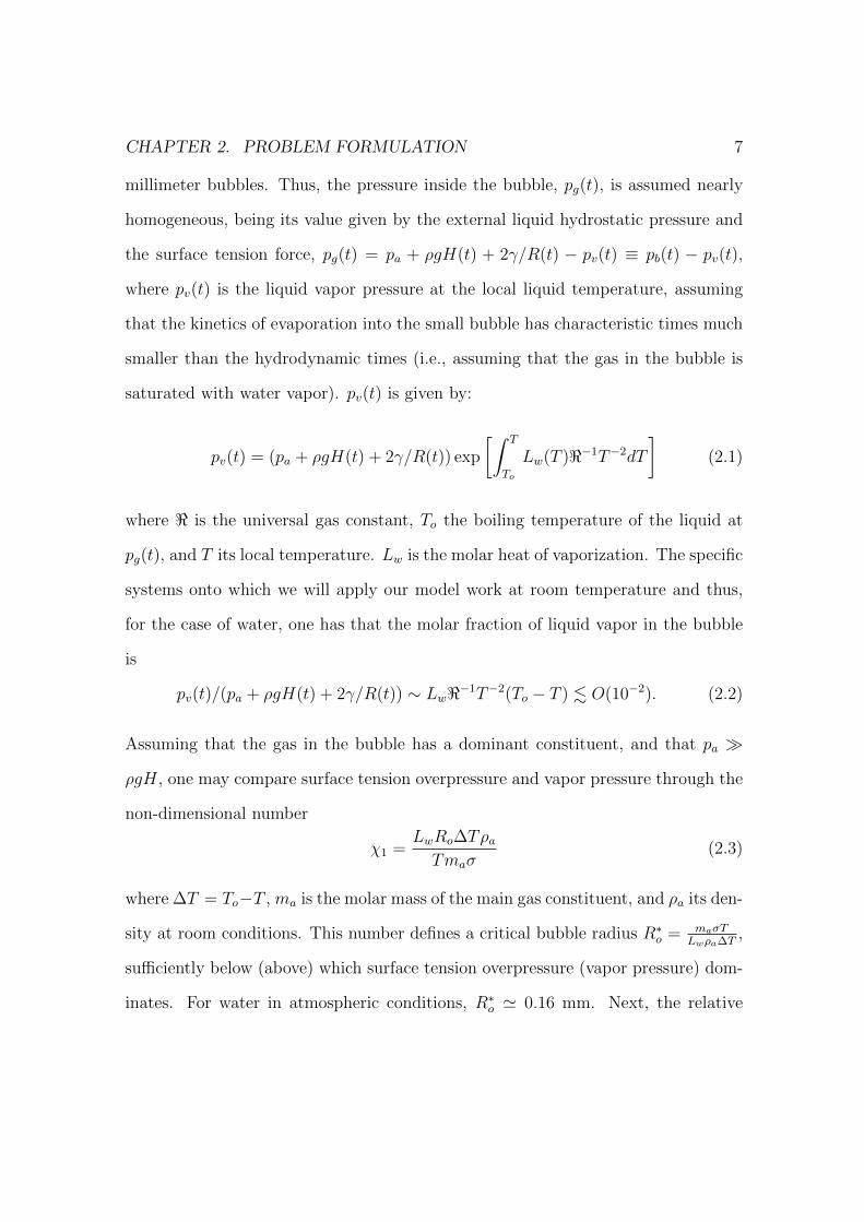
Figure 1 shows a sketch of the fluid configuration considered in this work. A spherical

gas bubble with initial radius Ro is released in a still liquid bath of density ρ and

viscosity µ from the bottom of a tube filled with liquid (water). the height of

the liquid column is Ho and its free surface is open to air at atmospheric pressure

pa. The initial volume concentration of gas dissolved in the liquid is c∞. Due to

the buoyancy force, the bubble rises at velocity V (t). Simultaneously, the bubble

exchanges gas with the liquid, and its radius R(t) varies on its way to the surface due

to either the change of liquid hydrostatic pressure and the dissolution of the gas in the

surrounding liquid. We assume that the surface tension γ between the gas and the

liquid is large enough to ensure that the bubble remains spherical during its ascent.

i. e. γ >> ρgR2o, where g is the acceleration of gravity. The bubble radius for which

buoyancy and surface tension forces become comparable is Rc =(

γ4ρg

)1/2

. For an air

bubble in water, that gives Rc = 1.35 mm. In this work, we will always consider sub-

6

CHAPTER 2. PROBLEM FORMULATION 7

millimeter bubbles. Thus, the pressure inside the bubble, pg(t), is assumed nearly

homogeneous, being its value given by the external liquid hydrostatic pressure and

the surface tension force, pg(t) = pa + ρgH(t) + 2γ/R(t) − pv(t) ≡ pb(t) − pv(t),

where pv(t) is the liquid vapor pressure at the local liquid temperature, assuming

that the kinetics of evaporation into the small bubble has characteristic times much

smaller than the hydrodynamic times (i.e., assuming that the gas in the bubble is

saturated with water vapor). pv(t) is given by:

pv(t) = (pa + ρgH(t) + 2γ/R(t)) exp

[∫ T

To

Lw(T )<−1T−2dT

](2.1)

where < is the universal gas constant, To the boiling temperature of the liquid at

pg(t), and T its local temperature. Lw is the molar heat of vaporization. The specific

systems onto which we will apply our model work at room temperature and thus,

for the case of water, one has that the molar fraction of liquid vapor in the bubble

is

pv(t)/(pa + ρgH(t) + 2γ/R(t)) ∼ Lw<−1T−2(To − T ) . O(10−2). (2.2)

Assuming that the gas in the bubble has a dominant constituent, and that pa

ρgH, one may compare surface tension overpressure and vapor pressure through the

non-dimensional number

χ1 =LwRo∆TρaTmaσ

(2.3)

where ∆T = To−T , ma is the molar mass of the main gas constituent, and ρa its den-

sity at room conditions. This number defines a critical bubble radius R∗o = maσTLwρa∆T

,

sufficiently below (above) which surface tension overpressure (vapor pressure) dom-

inates. For water in atmospheric conditions, R∗o ' 0.16 mm. Next, the relative


weight of the hydrostatic overpressure and the vapor pressure of the liquid can be

expressed by the non dimensional number

χ2 =ρgHomaT

ρaLw∆T(2.4)

The critical height sufficiently above (below) which hydrostatic pressure (vapor pres-

sure) dominates is given by H∗o = ρaLw∆TρgmaT

. Our working conditions (air in water,

atmospheric pressure) provide H∗o ' 46mm. Thus, both the liquid surface tension

and vapor pressures can be neglected in the analysis for bubble sizes larger than R∗o,

and rising bubble columns sufficiently larger than H∗o .

We use spherical coordinates (r, θ, ϕ) centered in the bubble and aligned with

the vertical tube (see Fig.2.1 (b)) to analyze the problem. In this frame of ref-

erence the liquid far-velocity field corresponds to a uniformly descending velocity

V (t). Moreover, since we consider relatively small bubbles, in principle we assume

dominance of viscous forces, although we will not dismiss inertia. Thus, the problem

is axisymmetric as far as the Reynolds number Reo = 2(

2ρ2gR3o

µ2

)1/2

remains smaller

than about 102, and henceforth we drop the coordinate ϕ.

2.2 Governing equations

To study the problem of the dissolved bubble rising in a still liquid, a derivation of

the differential form of continuity equation and momentum equation has been made

to get the final form of incompressible axisymmetric Navier-Stokes equations for the

liquid velocity v(r, θ; t) and dynamic pressure pd(r, θ; t) fields as follow:

The differential form of the continuity equation, for incompressible flow


Figure 2.1: Scheme of the problem.

∇ · v = 0, (2.5)

That writes in spherical coordinate as,

ur +2u

r+wθr

+w cot θ

r= 0, (2.6)

where subscripts r and θ denote the spatial derivatives with respect to r and with

respect to θ. The differential form of the momentum equation taking into account

the incompressible assumption and assuming constant viscosity is

ρ (vt + v · ∇v) = −∇pd + µ∇2v, (2.7)

In spherical coordinate for r-direction writes


ρ

(ut + uur +

wuθr− w2

r

)= −pdr+µ

(urr +

2urr

+uθθr2

+uθ cot θ

r2− 2u

r2− 2wθ

r2− 2w cot θ

r2

),

(2.8)

For θ-direction writes,

ρ(wt + uwr +

wwθr

+wu

r

)= −1

rpdθ+µ

(wrr +

2wrr

+wθθr2

+wθ cot θ

r2+

2uθr2− w

r2 sin2 θ

),

(2.9)

where subscript t denote the derivative with respect to the time. The incompressible

axisymmetric Navier-Stokes equations for the liquid velocity v(r, θ; t) and dynamic

pressure pd(r, θ; t) fields, are made dimensionless by using as characteristic quantities

Ro = R(0), and the terminal velocity for a bubble of radius Ro in the Stokes limit,

Uc = ρgR2o/(3µ) are

ur +2u

r+wθr

+w cot θ

r= 0, (2.10)

ut+uur+wuθr−w

2

r= −pdr+

1

Re

[urr +

2urr

+uθθr2

+uθ cot θ

r2− 2

(u

r2+wθr2

+w cot θ

r2

)],

(2.11)

wt+uwr+wwθr−wu

r= −pdθ

r+

1

Re

[wrr +

2wrr

+wθθr2

+wθ cot θ

r2− w

r2 sin2 θ+

2uθr2

],

(2.12)

where u/w is the radial/meridional velocity component and Re = ρUcRo/µ is the


Reynolds number. Note that the Stokes limit underestimates drag above Re ∼ 10,

and thus one should switch to a more realistic Reynolds as defined above, Reo, to

estimate the drag forces, where Reo = 241/2Re1/2. When Reo ∼ Re, both viscous

and inertia drag forces become comparable. The critical radius for which Reo = Re

is R∗∗o =(

72µρg

)1/3

. For an air bubble in water, this gives R∗∗ = 0.194 mm. Note that

the total pressure field, p, is the sum of the dynamic pressure and an hydrostatic

part, p = pd + ph, being

−∇ph + ρg − ρV = 0, (2.13)

ph =

∫ (ρg − ρV

)dz, (2.14)

Thus, the dimensionless hydrostatic pressure is,

ph = C +z

Fr− V z, (2.15)

where C is a constant, z the vertical coordinate, Fr = U2c /gRo the Froude number

and the symbol ˙ denotes time derivative. The last term in (2.15) is due to the use

of a non-inertial frame of reference.

We impose the equilibrium of tangential stress and the kinematic condition,

r(wr

)r

+uθr

= 0, (2.16)

wr −w

r+uθr

= 0, (2.17)


where uθ = 0 and the velocity in r-direction is constant with respect to θ

As a consequences, the boundary condition at the bubble surface, r = R(t),

u = R, and wr − w/r = 0. (2.18)

Additionally, it has to be considered the convection-diffusion equation to get

c(r, θ, t) which is the volume fraction of dissolved gas around the bubble,

The differential form of the convection-diffusion equation,

ct + v · ∇c = D∇2c, (2.19)

being each term,

v · ∇c = ucr +wcθr, (2.20)

∇2c =2crr

+ crr +cθ cot θ

r2+cθθr2, (2.21)

So that,

ct + ucr + wcθr

= D

(crr +

2crr

+cθθr2

+cot θcθr2

), (2.22)

The dimensionless convection-difussion equation for the volume concentration in

dimensionless form has is,

Φt + uΦr + wΦθ

r=

1

Pe

(Φrr +

2Φr

r+

Φθθ

r2+

cot θΦθ

r2

), (2.23)

where the dimensionless concentration of dissolved gas, Φ, is given by,

Φ =c− c∞cso − c∞

, (2.24)


being c(r, θ, t) the volume fraction of gas inside the liquid, cso = cs(0) the initial vol-

ume concentration at the surface of the bubble, c∞ the initial volume concentration

of gas dissolved in the liquid and Pe = RoUc/D the Peclet number, where D is the

gas-liquid molecular diffusivity.

The Henry’s law yields the partial pressure of the gas in the liquid p(r, θ, t) as a

function of the volume fraction of gas inside the liquid c(r, θ, t), c = KH p, where KH

is the Henry’s constant. This law allows to relate the volume concentration of gas at

the bubble surface, cs(t) with the gas pressure inside the bubble, cs(t) = KHpg(t) and

to calculate the partial pressure in the bulk of the liquid, p∞ = c∞/KH . Therefore,

the surface condition for Φ can be written as,

Φs =cs − c∞cso − c∞

=pg(t)− p∞pg(0)− p∞

= α1 + α2H(t), (2.25)

where

α1 =pa − p∞pref

and α2 =ρgRo

pref, (2.26)

being pref = pg(0)− p∞.

Away from the bubble, r → ∞, the velocity matches the external field and the

volume fraction the bulk volume fraction,

limr→∞

u = V (t) cos θ, limr→∞

w = −V (t) sin θ and limr→∞

Φ = 0. (2.27)

At any time,V (t), is computed by the integration of the equation of motion for

the spherical bubble, which neglecting the mass of the gas inside the bubble writes

as follow,


4

3πR3ρgV = −4

3πR3ρgg −Dh −Drag, (2.28)

where ρg is the density of the gas inside the bubble, Dh is the static part of the drag

and Drag it’s dynamic part,

Drag = 2πR2

∫ π

0

(−pdRe+ 2ur) cos θ sin θdθ . (2.29)

The static part is,

Dh =

∫Σ

ph~ndσ =

∫Ω

∇phdΩ, (2.30)

Dh =

∫Ω

(−ρg + ρV

)dΩ =

4

3πR3

(−ρg + ρV

), (2.31)

So,

4

3πR3ρgV =

4

3πR3

(ρg − ρgg − ρV

)−Drag, (2.32)

4

3πR3 (ρ+ ρg) V =

4

3πR3 (ρ− ρg) g −Drag, (2.33)

ρg is neglected since ρg ρ, resulting,

4

3πR3ρV =

4

3πR3ρg −Drag, (2.34)

Finally, the above equation in dimensionless form is,

V =1

Fr

(1− Drag

4πR3

). (2.35)

By applying the mass balance relationship at the bubble-liquid interface [5],


d

dt

(4

3πR3ρg

)= 2πR2ρlD

∫ π

0

cr sin θdθ, (2.36)

The dimensionless form of the previous equation is

2

3

Ro

to<T

(3R (Φspref + p∞) +RΦspref

)=cso − c∞Ro

ρlD

∫ π

0

Φr(r = R, θ) sin θdθ,

(2.37)

Or,

2

3pref

RoKHUcρlD<T

(3R (Φspref + p∞) +RΦspref

)=

∫ π

0

Φr(r = R, θ) sin θdθ, (2.38)

finally, the above equation writes in dimensionless form as,

2

3λ[3R(Φs + α3) +RΦs] = −Sh, (2.39)

where λ = RoBUc/D , being B = KH/(ρl<T ) and α3 = pp∞pref

. At each time the

Smith’ number Sh is computed numerically as

Sh = −∫ π

0

Φr(r = R, θ) sin θdθ. (2.40)

The derivative of the pressure with respect to time Φs = α2H results in,

3R(Φs + α3) + α2RH = −3Sh2λ

, (2.41)

Taking into account equation (2.25) and the equation for the evolution of H,


H = −V, (2.42)

it is obtained the equation for the time evolution of the radius of the bubble

R =−3/2λ−1Sh − α2RV

3(Φs + α3). (2.43)

2.3 Numerical procedure

Since the size of the bubble is changing with time, the following mapping was made

from the physical plane (r, θ, t) to the computational plane (η, ζ, τ),

η =r

R(t), ζ = θ, τ = t. (2.44)

Due to the large differences between the Re and Pe numbers present in the

experiments (Re ∼ 50 and Pe ∼ 30000) two different computational domains will be

used to solve the velocity and pressure fields and the gas concentration in the liquid

at the corresponding boundary layers of characteristic width δc and δv, respectively

(see figure 2.1.b). For the mechanical problem it is sufficient to truncate the radial

domain to an external radius, RV (t) = 30R(t) (ηv = 30), while for solving the

concentration boundary layer the domain is truncated at a much closer external

radius, Rc(t) = 200Pe−0.5R(t) (ηc = 200Pe−0.5).

The time procedure is described next. The time domain is discretized using a

fixed time step dτ . At given time, τN = Ndτ , the terminal velocity, V N , the height

of the bubble, HN and the radius of the bubble, RN are obtained from previous

times, τN−1 and τN−2, by discretizing in time equations (2.35), (2.42) and (2.43) at


time τN−1, using 2nd order central finite differences

V N = V N−2 + 2dτ1

Fr

(1− DragN−1

4π(RN−1)3

), (2.45)

HN = HN−2 − 2dτV N−1, (2.46)

RN = RN−2 + 2dτ−3/2λ−1ShN−1 − α2RV

N−1

3(ΦN−1s + α4)− α3/RN−1

. (2.47)

By the other hand, for the computation of the time evolution of Navier-Stokes

equations (2.10)-(2.12) and the convection-diffusion equation (2.23), a mixed implicit-

explicit second order projection scheme based on backwards differentiation is em-

ployed. [30] Spatial discretization in the (η, ζ) semiplanes employs nη Chebyshev

spectral collocation points in η, and nζ points in the ζ direction.

These schemes lead to the following set of Helmholtz-type equations:

(3Re

2dτ− 1

R2

∂2

∂η2− 2

ηR2

∂

∂η+

2

η2R2

)uN − 1

η2R2

(∂2

∂ζ2+ cotθ

∂

∂ζ

)uN = fu(2.48)(

3Re

2dτ− 1

R2

∂2

∂η2− 2

ηR2

∂

∂η

)wN − 1

η2R2

(∂2

∂ζ2+ cotζ

∂

∂ζ+

1

sin2ζ

)wN = fw(2.49)(

3Pe

2dτ− 1

R2

∂2

∂η2− 2

ηR2

∂

∂η

)cN − 1

η2R2

(∂2

∂ζ2+ cotζ

∂

∂ζ

)cN = fc(2.50)


where,

fu = Re

(−2convuN−1 + convuN−2 − 1

R

∂p

∂η+

4uN−1 − uN−2

2dτ

), (2.51)

fw = Re

(−2convwN−1 + convwN−2 − 1

ηR

∂p

∂ζ+

4wN−1 − wN−2

2dτ

), (2.52)

fc = Pe

(−2convcN−1 + convcN−2 +

4cN−1 − cN−2

2dτ

), (2.53)

and,

convu =1

R

(u− ηR

) ∂u∂η

+w

ηR

(∂u

∂ζ− w

)+

2

η2R2Re

(∂w

∂ζ+ wcotζ

)(2.54)

convw =1

R

(u− ηR

) ∂w∂η

+w

ηR

(∂w

∂ζ+ u

)− 2

η2R2Re

∂u

∂ζ. (2.55)

convc =1

R

(u− ηR

) ∂c∂η

+w

ηR

∂c

∂ζ. (2.56)

The previous equations is used to get the predicted values of velocity components

and concentration, where the symbol ˜ denotes predicted value, while to get the

pressure corrections, the poisson equation is discretized as follows:

(1

R2

∂2

∂η2+

2

ηR2

∂

∂η

)pN +

1

η2R2

(∂2

∂ζ2+ cotζ

∂

∂ζ

)pN =

1

2dτ

(1

ηR

∂wN

∂ζ+

1

R

∂uN

∂η+

2

ηRuN +

wN

ηRcotζ

).

(2.57)

This approach allows to use the matrix diagonalization method [31], whose com-

putational cost is of order nη × nζ ×min(nη, nζ), to solve the four Helmholtz-type

equations (2.48), (2.49), (2.50) and (2.57) resulting from the momentum and con-

centration equations and the Poisson equation needed to calculate the pressure cor-


rections. The nonlinear terms are evaluated using a pseudospectral method. [32] At

any time, the required velocity field in the convective term of the discretized concen-

tration equation, is obtained by interpolating the velocity field from the mechanical

domain to the concentration domain using a second order interpolation operator

along the η coordinate.

After getting the predicted values, the real value of (ut+1, wt+1, ct+1, pt+1) can be

obtained by solving the additional following equations:

pN = pN + pN−1. (2.58)

uN = uN − 2dτ

R

∂pN

∂η. (2.59)

wN = wN − 2dτ

ηR

∂pN

∂ζ. (2.60)

cN = cN . (2.61)

Note that both the spectral resolution used and the two different computational

domains considered, allow us to use a much less number of grid points that using

standards finite-differences in a single mesh. Therefore, we have carried out the

numerical simulations in a grid with nη = 60 and nζ = 25 for the cases presented

in this study. The time step employed in the simulations was ∆τ = 0.005, since

no significant differences in the temporal evolution of the flow were found by using

smaller time steps.

Chapter 3

Experimental setup

3.1 Apparatus Configuration

It has been prepared an experimental setup in order to validate the numerical code.

The experimental setup is sketched in figure 3.1. Bubbles of oxygen, liberated at the

bottom of a test section filled with quiescent distilled water, ascends freely through

the test section. The test section consists in a tube of 9 mm diameter and 116 cm

long being the upper extreme of the tube open to the air. The bubble generator is

a microfluidic flow-focusing device (Ingeniatrics Technologies). In the present flow

focusing configuration (shown in figure 3.2), a focusing stream of distilled water is

created by means a syringe pump (Harvard Apparatus PHD4400). The focusing

stream pinches off the gas meniscus giving up to the oxygen bubbles. The size of

the bubbles and its frequency of formation is controlled by a proper combination of

the flowrate of the focusing water and pressure of the gas in the meniscus. To this

end, the pressure of the gas is controlled by means of a pressure regulator (Swagelok

KLF) and a digital manometer (Digitron 2003P).

20

CHAPTER 3. EXPERIMENTAL SETUP 21

Distilled water from the pump

Oxygen from the pressure regulator

Optical Fiber

High Speed Video Camera

Optical Lenses

Z-axis Stage

3D Micrometer Screw

Bubble Generator

Test Section

Optical Table

Bubble

Figure 3.1: Configuration of the experiment.

The size of the bubbles is determined by analyzing its digital images. To this

end, images of the bubbles are acquired using a high-speed video camera (Redlake

MotionPro X4) equipped with a magnification zoom lens. The camera could be

displaced both horizontally and vertically using a triaxial translation stage to focus

the bubbles being them illuminated from the back by a cool white light provided by

an optical fiber (Schott KL2500 LCD). The test section is supported by a z-axis stage

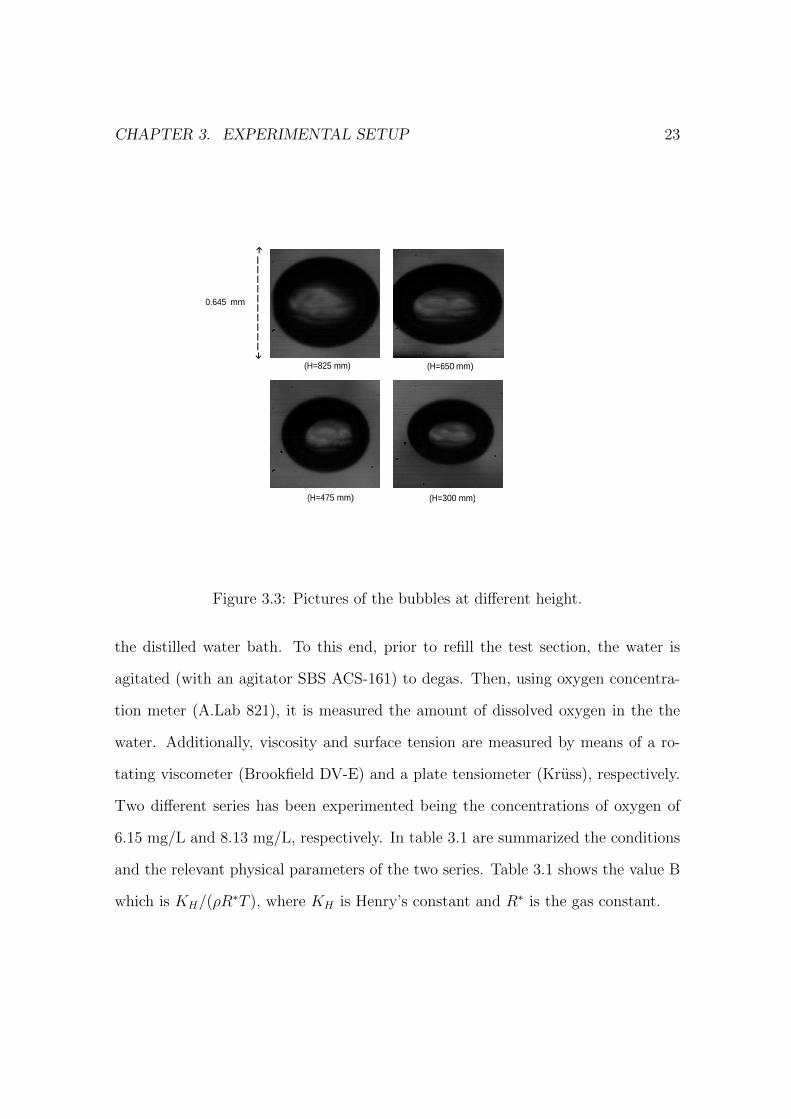
in order to select the height’s position of recording. Typical images of the bubbles

at different height are shown in figure 3.3. The bubbles, although spherical, appears

elliptical in the images due to the distortion created by the cylindrical geometry of

the test section. So, the radius of the droplet is determined by measuring in the


liquid

liquid

gas

Figure 3.2: The microfluidic flow-focusing device.

vertical direction. Pictures of 512x512 pixels at a rate of 5130 frames per second

are recorded. This rate of recording suffices to avoid blurring images of the bubbles.

Since the bubble generator does not produce perfectly monodisperse bubbles, for

each height a calibration process has been made and 20 measurements of the bubble’s

diameter has been taken for each test section and operating conditions. We have

assessed the spherical character of the bubbles in the present experimental conditions

by using a square glass test chamber for some experimental runs under the same

operating conditions as those of the more systematic study. In these selected runs,

in which any optical distortion is avoided, the maximum discrepancy between the

height and the width of the bubble as measured was 3.96 µm for a diameter of 468

µm.

3.2 Objective and Procedures

The objective of the experiment is to relate the size of the bubble with the distance

to the the free surface,i.e. the height. This relationship depends on the properties

of the quiescent liquid bath. So the fist step of the experiment is to characterize


|

|

|

|

|

|

|

|

|

|

0.645

mm

(H=825 mm)

(H=300 mm)

(H=650

mm)

(H=475 mm)

Figure 3.3: Pictures of the bubbles at different height.

the distilled water bath. To this end, prior to refill the test section, the water is

agitated (with an agitator SBS ACS-161) to degas. Then, using oxygen concentra-

tion meter (A.Lab 821), it is measured the amount of dissolved oxygen in the the

water. Additionally, viscosity and surface tension are measured by means of a ro-

tating viscometer (Brookfield DV-E) and a plate tensiometer (Kruss), respectively.

Two different series has been experimented being the concentrations of oxygen of

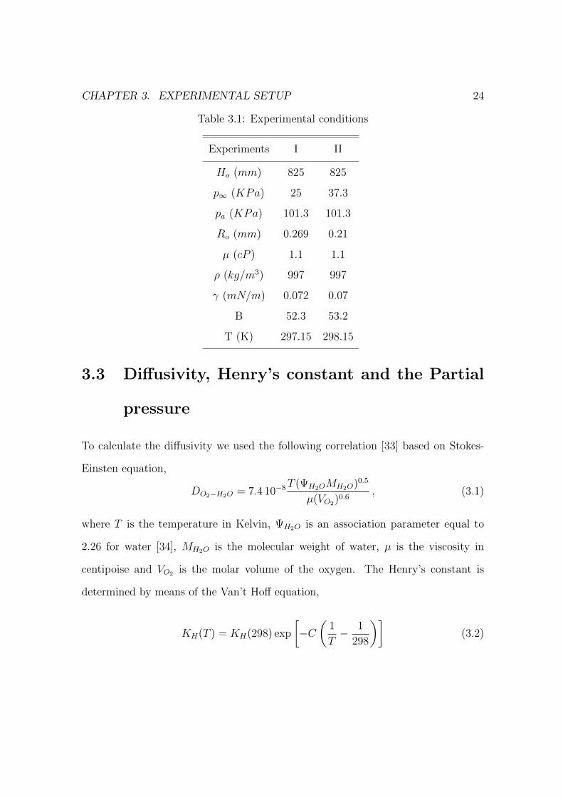
6.15 mg/L and 8.13 mg/L, respectively. In table 3.1 are summarized the conditions

and the relevant physical parameters of the two series. Table 3.1 shows the value B

which is KH/(ρR∗T ), where KH is Henry’s constant and R∗ is the gas constant.


Table 3.1: Experimental conditions

Experiments I II

Ho (mm) 825 825

p∞ (KPa) 25 37.3

pa (KPa) 101.3 101.3

Ro (mm) 0.269 0.21

µ (cP ) 1.1 1.1

ρ (kg/m3) 997 997

γ (mN/m) 0.072 0.07

B 52.3 53.2

T (K) 297.15 298.15

3.3 Diffusivity, Henry’s constant and the Partial

pressure

To calculate the diffusivity we used the following correlation [33] based on Stokes-

Einsten equation,

DO2−H2O = 7.4 10−8T (ΨH2OMH2O)0.5

µ(VO2)0.6

, (3.1)

where T is the temperature in Kelvin, ΨH2O is an association parameter equal to

2.26 for water [34], MH2O is the molecular weight of water, µ is the viscosity in

centipoise and VO2 is the molar volume of the oxygen. The Henry’s constant is

determined by means of the Van’t Hoff equation,

KH(T ) = KH(298) exp

[−C

(1

T− 1

298

)](3.2)


where Henry’s constant for oxygen in water at 298 K is equal to 769.23 L.atmmole

and C

is a constant equal to 1700 for oxygen. Finally, the partial pressure of the oxygen

in the bath is, using Henry’s law,

p∞ = KHc∞. (3.3)

where c∞ is the oxygen concentration in the bath.

Chapter 4

Results and discussion

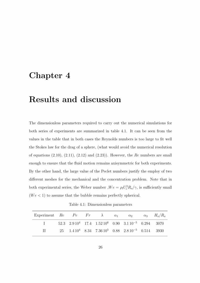
The dimensionless parameters required to carry out the numerical simulations for

both series of experiments are summarized in table 4.1. It can be seen from the

values in the table that in both cases the Reynolds numbers is too large to fit well

the Stokes law for the drag of a sphere, (what would avoid the numerical resolution

of equations (2.10), (2.11), (2.12) and (2.23)). However, the Re numbers are small

enough to ensure that the fluid motion remains axisymmetric for both experiments.

By the other hand, the large value of the Peclet numbers justify the employ of two

different meshes for the mechanical and the concentration problem. Note that in

both experimental series, the Weber number ,We = ρlU2cRo/γ, is sufficiently small

(We < 1) to assume that the bubble remains perfectly spherical.

Table 4.1: Dimensionless parameters

Experiment Re Pe Fr λ α1 α2 α3 Ho/Ro

I 52.3 2.9 104 17.4 1.52 106 0.90 3.1 10−5 0.294 3070

II 25 1.4 104 8.34 7.36 105 0.88 2.8 10−5 0.514 3930

26

CHAPTER 4. RESULTS AND DISCUSSION 27

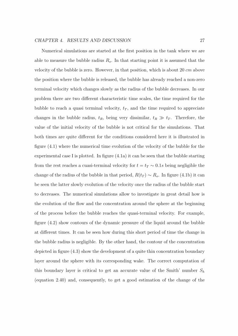
Numerical simulations are started at the first position in the tank where we are

able to measure the bubble radius Ro. In that starting point it is assumed that the

velocity of the bubble is zero. However, in that position, which is about 20 cm above

the position where the bubble is released, the bubble has already reached a non-zero

terminal velocity which changes slowly as the radius of the bubble decreases. In our

problem there are two different characteristic time scales, the time required for the

bubble to reach a quasi terminal velocity, tT , and the time required to appreciate

changes in the bubble radius, tR, being very dissimilar, tR tT . Therefore, the

value of the initial velocity of the bubble is not critical for the simulations. That

both times are quite different for the conditions considered here it is illustrated in

figure (4.1) where the numerical time evolution of the velocity of the bubble for the

experimental case I is plotted. In figure (4.1a) it can be seen that the bubble starting

from the rest reaches a cuasi-terminal velocity for t = tT ∼ 0.1s being negligible the

change of the radius of the bubble in that period, R(tT ) ∼ Ro. In figure (4.1b) it can

be seen the latter slowly evolution of the velocity once the radius of the bubble start

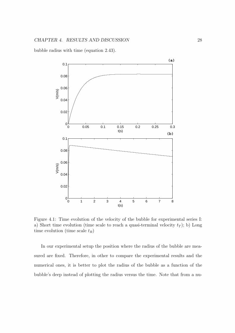
to decreases. The numerical simulations allow to investigate in great detail how is

the evolution of the flow and the concentration around the sphere at the beginning

of the process before the bubble reaches the quasi-terminal velocity. For example,

figure (4.2) show contours of the dynamic pressure of the liquid around the bubble

at different times. It can be seen how during this short period of time the change in

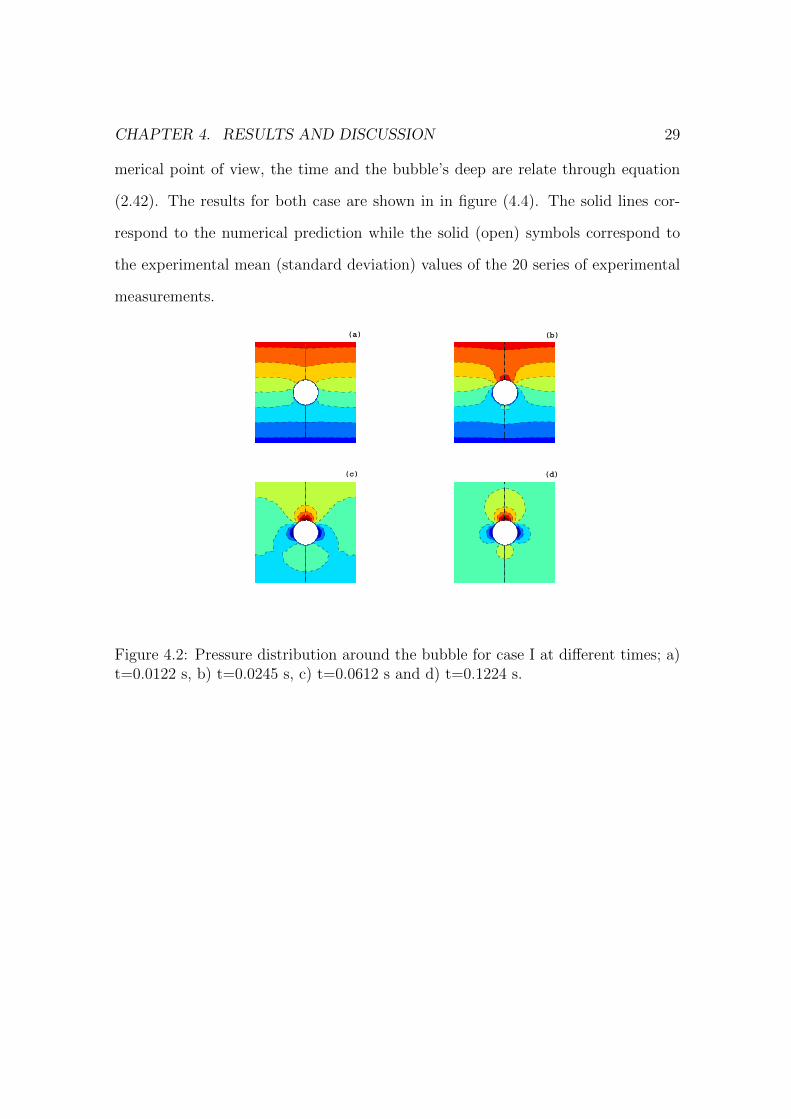
the bubble radius is negligible. By the other hand, the contour of the concentration

depicted in figure (4.3) show the development of a quite thin concentration boundary

layer around the sphere with its corresponding wake. The correct computation of

this boundary layer is critical to get an accurate value of the Smith’ number Sh

(equation 2.40) and, consequently, to get a good estimation of the change of the


bubble radius with time (equation 2.43).

0 0.05 0.1 0.15 0.2 0.25 0.30

0.02

0.04

0.06

0.08

0.1

t(s)

V(m

/s)

0 1 2 3 4 5 6 7 80

0.02

0.04

0.06

0.08

0.1

t(s)

V(m

/s)

(b)

(a)

Figure 4.1: Time evolution of the velocity of the bubble for experimental series I:a) Short time evolution (time scale to reach a quasi-terminal velocity tT ); b) Longtime evolution (time scale tR)

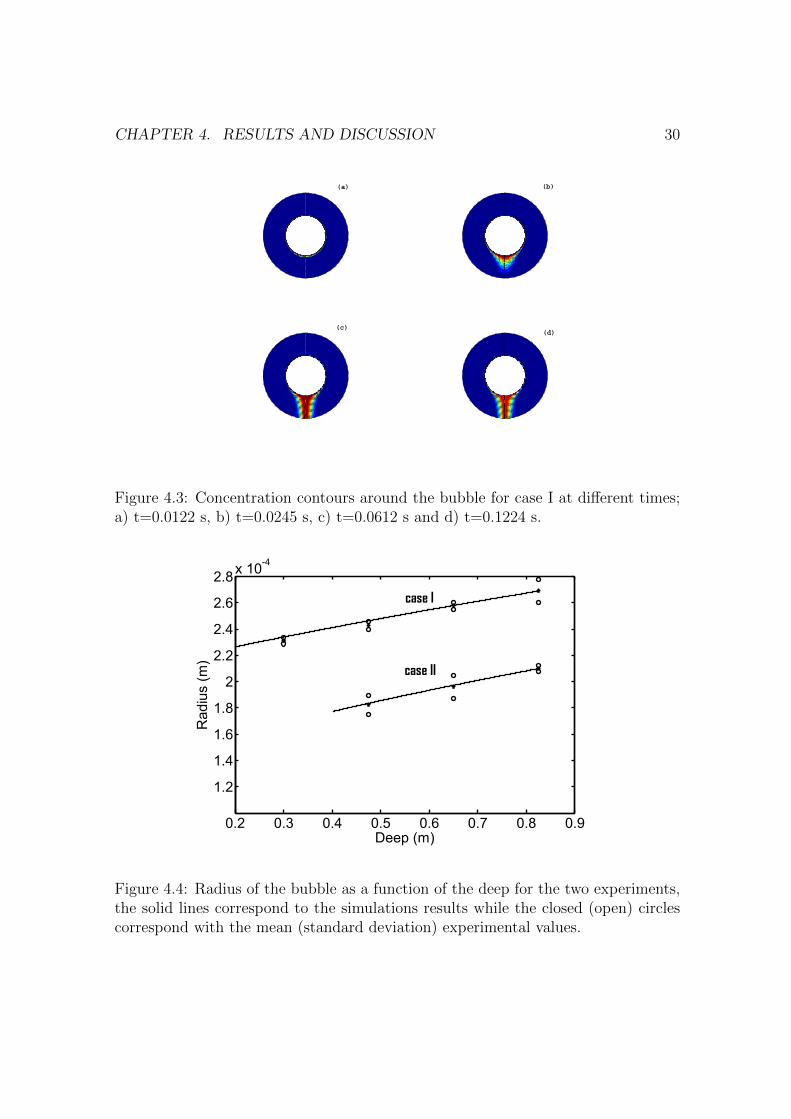
In our experimental setup the position where the radius of the bubble are mea-

sured are fixed. Therefore, in other to compare the experimental results and the

numerical ones, it is better to plot the radius of the bubble as a function of the

bubble’s deep instead of plotting the radius versus the time. Note that from a nu-


merical point of view, the time and the bubble’s deep are relate through equation

(2.42). The results for both case are shown in in figure (4.4). The solid lines cor-

respond to the numerical prediction while the solid (open) symbols correspond to

the experimental mean (standard deviation) values of the 20 series of experimental

measurements.

(c)

(a) (b)

(d)

Figure 4.2: Pressure distribution around the bubble for case I at different times; a)t=0.0122 s, b) t=0.0245 s, c) t=0.0612 s and d) t=0.1224 s.


(a) (b)

(c)(d)

Figure 4.3: Concentration contours around the bubble for case I at different times;a) t=0.0122 s, b) t=0.0245 s, c) t=0.0612 s and d) t=0.1224 s.

0.2 0.3 0.4 0.5 0.6 0.7 0.8 0.9

1.2

1.4

1.6

1.8

2

2.2

2.4

2.6

2.8x 10-4

Deep (m)

Rad

ius

(m)

case II

case I

Figure 4.4: Radius of the bubble as a function of the deep for the two experiments,the solid lines correspond to the simulations results while the closed (open) circlescorrespond with the mean (standard deviation) experimental values.

Chapter 5

Summary, conclusions and Future

Works

In the present work the following achievements has been obtained,

A tracking-interface numerical method was used to achieve this work. The

method has been applied to study of the isothermal dissolution of small single

rising bubble.

The key elements of the method are the use of a frame of reference moving

with the bubble and the application of different meshes to solve the mechanical

and mass-diffusion problems.

An experiment of a small oxygen bubble rising in water has been carried out

with remarkable agreement to the numerical model.

In future works it is intended,

1. To develop a code for the linear stability study of convective - absolute transi-

31

CHAPTER 5. SUMMARY, CONCLUSIONS AND FUTURE WORKS 32

tion of gas streams which are injected into a T-shaped intersection of a rectan-

gular channel that carries a liquid stream (rivulets). Characterize parametric

regions where the formation of stable rivulets occur.

2. To get information from the stability study to perform 3D numerical sim-

ulations with a method of monitoring the VOF to characterize gas - liquid

geometric configurations that allow to obtain mono-dispersed bubbles smaller

than the width of the channel.

3. To design an experimental setup for studying rivulets gaseous stream driven

by a liquid -based cell using planar Hele- Shaw type.

4. To design and construct of an experiment of nebulizing nanosized particulate

matter to the atmosphere with the Blurring FLow technique.

List of Figures

2.1 Scheme of the problem. . . . . . . . . . . . . . . . . . . . . . . . . . . 9

3.1 Configuration of the experiment. . . . . . . . . . . . . . . . . . . . . . 21

3.2 The microfluidic flow-focusing device. . . . . . . . . . . . . . . . . . . 22

3.3 Pictures of the bubbles at different height. . . . . . . . . . . . . . . . 23

4.1 Time evolution of the velocity of the bubble for experimental series I:

a) Short time evolution (time scale to reach a quasi-terminal velocity

tT ); b) Long time evolution (time scale tR) . . . . . . . . . . . . . . . 28

4.2 Pressure distribution around the bubble for case I at different times;

a) t=0.0122 s, b) t=0.0245 s, c) t=0.0612 s and d) t=0.1224 s. . . . . 29

4.3 Concentration contours around the bubble for case I at different times;

a) t=0.0122 s, b) t=0.0245 s, c) t=0.0612 s and d) t=0.1224 s. . . . . 30

4.4 Radius of the bubble as a function of the deep for the two experi-

ments, the solid lines correspond to the simulations results while the

closed (open) circles correspond with the mean (standard deviation)

experimental values. . . . . . . . . . . . . . . . . . . . . . . . . . . . 30

33

List of Tables

3.1 Experimental conditions . . . . . . . . . . . . . . . . . . . . . . . . . 24

4.1 Dimensionless parameters . . . . . . . . . . . . . . . . . . . . . . . . 26

34

Bibliography

[1] D. W. Moore. The velocity of rise of distorted gas bubbles in a liquid of small

viscosity. J. Fluid Mech., 23:749–766, 1965.

[2] P. C. Duineveld. Rise velocity and shape of bubbles in pure water at high

reynolds number. Journal of Fluid Mechanics, 292:325–332, 1995.

[3] G. Mougin and J. Magnaudet. Path instability of a rising bubble. Physical

Review Letters, 88:145021–145024, 2002.

[4] C. Martınez-Bazan, J. L. Montanes, and J. C. Lasheras. Statistical description

of the bubble cloud resulting from the injection of air into a turbulent water

jet. International Journal of Multiphase Flow, 28:597–615, 2002.

[5] Fumio Takemura and Akira Yabe. Gas dissolution process of spherical rising

gas bubble. Chemical Engineering Science, 53(15):2691–2699, 1998.

[6] F. Takemura and A. Yabe. Rising speed and dissolution rate of a carbon dioxide

bubble in slightly contaminated water. Journal of Fluid Mechanics, 378:319–

334, 1999.

35

BIBLIOGRAPHY 36

[7] D.F. McGinnis, J. Greinert, Y. Artemov, S.E. Beaubien, and A. Wuest. Fate

of rising methane bubbles in stratified waters: How much methane reaches the

atmosphere? Journal of Geophysical Research C: Oceans, 111:C09007, 2006.

[8] H. Ding, P. D. M. Spelt, and C. Shu. Diffuse interface model for incompressible

two-phase flows with large density ratios. Journal of Computational Physics,

226:2078–2095, 2007.

[9] M.G. Gerritsen and L.J. Durlofsky. Modeling fluid flow in oil reservoirs. Annual

Review of Fluid Mechanics, 37:211–238, 2005.

[10] A. Shokrollahi, M. Arabloo, F. Gharagheizi, and A.H. Mohammadi. Intelligent

model for prediction of co2 - reservoir oil minimum miscibility pressure. Fuel,

112:375–384, 2013.

[11] V.L. Singleton and J.C. Little. Designing hypolimnetic aeration and oxygena-

tion systems - a review. Environmental Science and Technology, 40:7512–7520,

2006.

[12] D.N. Rao and J.I. Lee. Determination of gas-oil miscibility conditions by inter-

facial tension measurements. Journal of Colloid and Interface Science, 262:474–

482, 2003.

[13] Saeid Vafaei and Dongsheng Wen. Bubble formation on a submerged micronoz-

zle. Colloid and Interface Science, 343:291–297, 2010.

[14] A. M. Ganan-Calvo and J. M. Gordillo. Perfectly monodisperse microbubbling

by capillary flow focusing. Phys. Rev. Lett., 87:274501, 2001.

BIBLIOGRAPHY 37

[15] P. Garstecki, I. Gitlin, W. DiLuzio, G. M. Whitesides, E. Kumacheva, and

H. A. Stone. Formation of monodisperse bubbles in a microfluidic flow-focusing

device. Appl. Phys. Lett., 85:2649–2651, 2004.

[16] T. Cubaud, M. Tatineni, X. Zhong, and C.-M. Ho. Bubble dispenser in mi-

crofluidic devices. Phys. Rev. E, 72:037302, 2005.

[17] P. Garstecki, A. M. Ganan-Calvo, and G. M. Whitesides. Formation of bubbles

and droplets in microfluidic systems. Bull. Polish Ac.: Tech. Sci., 53:361–372,

2005.

[18] A. M. Ganan-Calvo, M. A. Herrada, and P. Garstecki. Bubbling in unbounded

coflowing liquids. Phys. Rev. Lett., 96:124504, 2006.

[19] Michinao Hashimoto, Sergey S. Shevkoplyas, Beata Zasonska, Tomasz Szym-

borski, Piotr Garstecki, and George M. Whitesides. Formation of bubbles and

droplets in parallel, coupled flow-focusing geometries. Small, 4:1795–1805, 2008.

[20] M. A. Herrada and A. M. Ganan-Calvo. Swirl flow focusing: A novel proce-

dure for the massive production of monodisperse microbubbles. Phys. Fluids,

21:042003, 2009.

[21] M. A. Herrada, A. M. Ganan-Calvo, and J. M. Lopez-Herrera. Generation

of small mono-disperse bubbles in axisymmetric t-junction: The role of swirl.

Phys. Fluids, 23:072004, 2011.

[22] M. A. Herrada, A. M. Ganan-Calvo, and J. M. Montanero. Theoretical inves-

tigation of a technique to produce microbubbles by a microfluidic t junction.

Phys. Rev. E, 88:033027, 2013.

BIBLIOGRAPHY 38

[23] C. S. Smith. On blowing bubbles for bragg’s dynamic crystal model. J. Appl.

Phys., 20:631–632, 1949.

[24] A. M. Ganan-Calvo. Perfectly monodisperse microbubbling by capillary flow

focusing: An alternate physical description and universal scaling. Phys. Rev.

E, 69:027301, 2004.

[25] T. Thorsen, R.W. Roberts, F. H. Arnold, and S. R. Quake. Dynamic pattern

formation in a vesicle-generating microfluidic device. Phys. Rev. Lett., 86:4163,

2001.

[26] A. Gunther, S. A. Khan, M. Thalmann, F. Trachsel, and K. F. Jensen. Trans-

port and reaction in microscale segmented gas–liquid flow. Lab Chip, 4:278,

2004.

[27] P. Garstecki, M. J. Fuerstman, S. K. Sia, and G. M. Whitesides. Formation

of droplets and bubbles in a microfluidic t-junction—scaling and mechanism of

break-up. Lab Chip, 6:437–446, 2006.

[28] T. Cubaud and C.-M. Ho. Transport of bubbles in square microchannels. Phys.

Fluids, 16:4575–4585, 2004.

[29] Chain-Nan Yung and Kenneth J De Witt. A numerical study of parameters

affecting gas bubble dissolution. Journal of Colloid and Interface Science,

127:442–452, 1988.

[30] J.M.Lopez, F. Marques, and J. Shen. An eficient spectral-projection method

for the navier-stokes equations in cylindrical geometries ii. three dimensional

cases. J. Comput. Phys., 176:401, 2002.

BIBLIOGRAPHY 39

[31] R. E. Lynch, J. R. Rice, and D. H. Thomas. Direct solution of partial differential

equations by tensor product methods. Numer. Math., 6:85, 1964.

[32] C. Canuto, M.Y. Hussaini, A. Quarteroni, and T.A. Zang. Spectral methods in

fluid dynamics. Springer-Verlag., 1988.

[33] P. Chang and C.R. Wilke. Some measurements of diffusion in liquids. The

Journal of Physical Chemistry, 59(7):592–596, 1955.

[34] John M. Prausnitz Robert C. Reid and Thomas K. Sherwood. The properties

of gases and liquids. AIChE Journal, 24:1142, 1978.

Documents

Disoluci on de Burbujas Liberadas en un Bano~ L quido Isotermobibing.us.es/proyectos/abreproy/70535/fichero/Trabajo+Fin+de+Máster... · Chapter 1 Introduction 1.1 Motivation and