DISLIN 8 - lab.demog.berkeley.edu · DISLIN 8.1 A Data Plotting Extension for the Programming Language Python by Helmut Michels

D I S L I N 8.1

A Data Plotting Extension

for the

Programming Language

Python

by

Helmut Michels

c� Helmut Michels, Max-Planck-Institut f¨ur Aeronomie, Katlenburg-Lindau 1997 - 2003

All rights reserved.

Contents

1 Overview 11.1 Introduction . .. . . . . . . . . . . . . . . . . . . . . . . . . . . . . . . . . . . . . . . 11.2 DISLIN Features . . . . . . . . . . . . . . . . . . . . . . . . . . . . . . . . . . . . . . 11.3 Passing Parameters from Python to DISLIN Routines . . .. . . . . . . . . . . . . . . . 21.4 Quickplots . . .. . . . . . . . . . . . . . . . . . . . . . . . . . . . . . . . . . . . . . . 21.5 FTP Sites, DISLIN Home Page. . . . . . . . . . . . . . . . . . . . . . . . . . . . . . . 31.6 Reporting Bugs. . . . . . . . . . . . . . . . . . . . . . . . . . . . . . . . . . . . . . . 3

2 Quickplots 52.1 The PLOT Function. . . . . . . . . . . . . . . . . . . . . . . . . . . . . . . . . . . . . 52.2 The SCATTR Function . .. . . . . . . . . . . . . . . . . . . . . . . . . . . . . . . . . 52.3 The PLOT3 Function . . .. . . . . . . . . . . . . . . . . . . . . . . . . . . . . . . . . 62.4 The SURF3 Function . . .. . . . . . . . . . . . . . . . . . . . . . . . . . . . . . . . . 62.5 The SURFACE Function .. . . . . . . . . . . . . . . . . . . . . . . . . . . . . . . . . 62.6 The SURSHADE Function. . . . . . . . . . . . . . . . . . . . . . . . . . . . . . . . . 62.7 The CONTOUR Function .. . . . . . . . . . . . . . . . . . . . . . . . . . . . . . . . . 62.8 The CONSHADE Function. . . . . . . . . . . . . . . . . . . . . . . . . . . . . . . . . 72.9 Scaling of Quickplots . . .. . . . . . . . . . . . . . . . . . . . . . . . . . . . . . . . . 72.10 Quickplot Variables. . . . . . . . . . . . . . . . . . . . . . . . . . . . . . . . . . . . . 8

A Short Description of DISLIN Routines 11A.1 Initialization and Introductory Routines. . . . . . . . . . . . . . . . . . . . . . . . . . 11A.2 Termination and Parameter Resetting .. . . . . . . . . . . . . . . . . . . . . . . . . . . 12A.3 Plotting Text and Numbers. . . . . . . . . . . . . . . . . . . . . . . . . . . . . . . . . 12A.4 Fonts . . . . . . . . . . . . . . . . . . . . . . . . . . . . . . . . . . . . . . . . . . . . 13A.5 Symbols. . . . . . . . . . . . . . . . . . . . . . . . . . . . . . . . . . . . . . . . . . . 14A.6 Axis Systems .. . . . . . . . . . . . . . . . . . . . . . . . . . . . . . . . . . . . . . . 14A.7 Secondary Axes. . . . . . . . . . . . . . . . . . . . . . . . . . . . . . . . . . . . . . . 15A.8 Modification of Axes . . .. . . . . . . . . . . . . . . . . . . . . . . . . . . . . . . . . 15A.9 Axis System Titles . . . . . . . . . . . . . . . . . . . . . . . . . . . . . . . . . . . . . 16A.10 Plotting Data Points. . . . . . . . . . . . . . . . . . . . . . . . . . . . . . . . . . . . . 16A.11 Legends. . . . . . . . . . . . . . . . . . . . . . . . . . . . . . . . . . . . . . . . . . . 17A.12 Line Styles and Shading Patterns . . .. . . . . . . . . . . . . . . . . . . . . . . . . . . 18A.13 Cycles . . . . . . . . . . . . . . . . . . . . . . . . . . . . . . . . . . . . . . . . . . . . 18A.14 Base Transformations . . .. . . . . . . . . . . . . . . . . . . . . . . . . . . . . . . . . 18A.15 Shielding . . .. . . . . . . . . . . . . . . . . . . . . . . . . . . . . . . . . . . . . . . 19A.16 Parameter Requesting Routines. . . . . . . . . . . . . . . . . . . . . . . . . . . . . . . 19A.17 Elementary Plot Routines .. . . . . . . . . . . . . . . . . . . . . . . . . . . . . . . . . 20A.18 Conversion of Coordinates. . . . . . . . . . . . . . . . . . . . . . . . . . . . . . . . . 21A.19 Utility Routines . . . . . . . . . . . . . . . . . . . . . . . . . . . . . . . . . . . . . . . 21A.20 Date Routines .. . . . . . . . . . . . . . . . . . . . . . . . . . . . . . . . . . . . . . . 22A.21 Cursor Routines. . . . . . . . . . . . . . . . . . . . . . . . . . . . . . . . . . . . . . . 22

i

A.22 Bar Graphs . . . . . . . . . . . . . . . . . . . . . . . . . . . . . . . . . . . . . . . . . 23A.23 Pie Charts. . . . . . . . . . . . . . . . . . . . . . . . . . . . . . . . . . . . . . . . . . 23A.24 Coloured 3-D Graphics. . . . . . . . . . . . . . . . . . . . . . . . . . . . . . . . . . . 24A.25 3-D Graphics . . .. . . . . . . . . . . . . . . . . . . . . . . . . . . . . . . . . . . . . 25A.26 Geographical Projections . . .. . . . . . . . . . . . . . . . . . . . . . . . . . . . . . . 26A.27 Contouring . . . . . . . . . . . . . . . . . . . . . . . . . . . . . . . . . . . . . . . . . 27A.28 Image Routines . .. . . . . . . . . . . . . . . . . . . . . . . . . . . . . . . . . . . . . 27A.29 Window Routines .. . . . . . . . . . . . . . . . . . . . . . . . . . . . . . . . . . . . . 28A.30 Widget Routines .. . . . . . . . . . . . . . . . . . . . . . . . . . . . . . . . . . . . . 28A.31 DISLIN Quickplots . . . . . . . . . . . . . . . . . . . . . . . . . . . . . . . . . . . . . 30A.32 MPAe Emblem . .. . . . . . . . . . . . . . . . . . . . . . . . . . . . . . . . . . . . . 30

B Examples 31B.1 Demonstration of CURVE . .. . . . . . . . . . . . . . . . . . . . . . . . . . . . . . . 32B.2 Polar Plots. . . . . . . . . . . . . . . . . . . . . . . . . . . . . . . . . . . . . . . . . . 34B.3 Symbols .. . . . . . . . . . . . . . . . . . . . . . . . . . . . . . . . . . . . . . . . . . 36B.4 Logarithmic Scaling. . . . . . . . . . . . . . . . . . . . . . . . . . . . . . . . . . . . . 38B.5 Interpolation Methods. . . . . . . . . . . . . . . . . . . . . . . . . . . . . . . . . . . . 40B.6 Line Styles . . . . . . . . . . . . . . . . . . . . . . . . . . . . . . . . . . . . . . . . . 42B.7 Legends .. . . . . . . . . . . . . . . . . . . . . . . . . . . . . . . . . . . . . . . . . . 44B.8 Shading Patterns (AREAF) . .. . . . . . . . . . . . . . . . . . . . . . . . . . . . . . . 46B.9 Vectors . . . . . . . . . . . . . . . . . . . . . . . . . . . . . . . . . . . . . . . . . . . 48B.10 3-D Colour Plot . .. . . . . . . . . . . . . . . . . . . . . . . . . . . . . . . . . . . . . 50B.11 Surface Plot. . . . . . . . . . . . . . . . . . . . . . . . . . . . . . . . . . . . . . . . . 52B.12 Surface Plot. . . . . . . . . . . . . . . . . . . . . . . . . . . . . . . . . . . . . . . . . 54B.13 Contour Plot. . . . . . . . . . . . . . . . . . . . . . . . . . . . . . . . . . . . . . . . . 56B.14 Shaded Contour Plot. . . . . . . . . . . . . . . . . . . . . . . . . . . . . . . . . . . . 59B.15 Pie Charts. . . . . . . . . . . . . . . . . . . . . . . . . . . . . . . . . . . . . . . . . . 62B.16 World Coastlines and Lakes .. . . . . . . . . . . . . . . . . . . . . . . . . . . . . . . 64

ii

Chapter 1

Overview

1.1 Introduction

This manual describes a data plotting extension for the interpreted, object-oriented programming lan-guage Python. The plotting extension is based on the data plotting library DISLIN that is available forseveral C, Fortran 77 and Fortran 90 compilers.

DISLIN is a high-level plotting library that contains subroutines and functions for displaying data graph-icallly as curves, bar graphs, pie charts, 3-D colour plots, surfaces, contours and maps. The librarycontains about 400 plotting and parameter setting routines which are now available from Python. Somequickplots are also added to the DISLIN module for displaying curves, surfaces and contours with onecommand.

1.2 DISLIN Features

The following features are supported by DISLIN:

- Several output formats can be selected such as X11, PostScript, PDF, CGM, Prescribe, TIFF andHPGL.

- 9 software fonts are available where each font provides 6 alphabets and special european charac-ters. Hardware fonts for PostScript printers and X11 and Windows displays can also be used.

- Plotting of two- and three-dimensional axis systems. Axes can be linearly or logarithmically scaledand labeled with linear, logarithmic, date, time, map and user-defined formats.

- Plotting of curves. Several curves can appear in one axis system and can be differentiated bycolour, line style and pattern. Multiple axis systems can be displayed on one page.

- Plotting of legends.

- Elementary plot routines for lines, vectors and outlined or filled regions such as rectangles, circles,arcs, ellipses and polygons.

- Shielded regions can be defined.

- Business graphics.

- 3-D colour graphics.

- 3-D graphics.

- Elementary image routines.

1

- Geographical projections and plotting of maps.

- Contouring.

- A PostScript manual of DISLIN is available.

1.3 Passing Parameters from Python to DISLIN Routines

The passing of parameters from Python to DISLIN routines is not so strict as in other programminglanguages. The following rules are applied:

- Parameters can be passed from Python to DISLIN routines as variables, constants and expressions.

- String constants must be enclosed in a pair of either apostrophes or quotation marks.

- Floatingpoint parameters can be passed from Python as integer and floatingpoint numbers.

- Integer parameters can be passed from Python as integer and floatingpoint numbers. If a floating-point number is passed for an integer parameter, the fractional part of the floatingpoint numberwill be truncated.

- Floatingpoint arrays can be passed from Python as floatingpoint and integer lists. They were copiedto 32 bit C arrays before they are passed to DISLIN routines.

- Integer arrays must be passed as integer lists.

- Memory must be allocated for Arrays that are used from DISLIN routines as output parameters.For example, they can be created with the Python command ’range’.

Note: Normally, the number and meaning of parameters passed to DISLIN routines areidentical with the syntax description of the routines in the DISLIN manual. DISLINroutines that return one ore more scalars are implemented for Python as functionsthat return a tuple of scalars. For example, the statement ’nw,nh = getpag ()’ returnsthe page size.

1.4 Quickplots

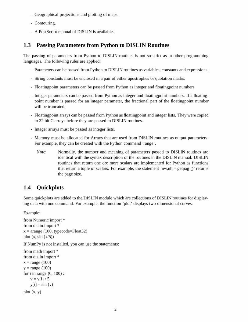
Some quickplots are added to the DISLIN module which are collections of DISLIN routines for display-ing data with one command. For example, the function ’plot’ displays two-dimensional curves.

Example:

from Numeric import *from dislin import *x = arange (100, typecode=Float32)plot (x, sin (x/5))

If NumPy is not installed, you can use the statements:

from math import *from dislin import *x = range (100)y = range (100)for i in range (0, 100) :

v = y[i] / 5.y[i] = sin (v)

plot (x, y)

2

Figure 2.1: Example of the plot Function

1.5 FTP Sites, DISLIN Home Page

The DISLIN software is available via ftp anonymous from the following sites:

ftp://ftp.gwdg.de/pub/grafik/dislinftp://unix1.mpae.gwdg.de/pub/dislin

The DISLIN Home Page is:

http://www.dislin.de

The Python Home Page is:

http://www.python.org

1.6 Reporting Bugs

DISLIN is well tested by many users and should be very bug free. However, no software is perfect. Ifyou have any problems with DISLIN, contact the author:

Helmut MichelsMax-Planck-Institut fuer AeronomieD-37191 Katlenburg-Lindau, Max-Planck-Str. 2, GermanyE-Mail: [email protected].: +49 5556 979 334Fax: +49 5556 979 240

3

4

Chapter 2

Quickplots

This chapter presents quickplots that are collections of DISLIN routines to display data with one com-mand.

The following rules are applied to quickplots:

- Quickplots call DISINI automatically if it is not called before. METAFL (’XWIN’) will be usedin quickplots if METAFL is not used before.

- On window terminals, there are no calls to ENDGRF and DISFIN in quickplots, they let DISLINin level 2 or 3. If the variable ERASE is set to 0, following quickplots will overwrite the graphicswindow without erasing the window.

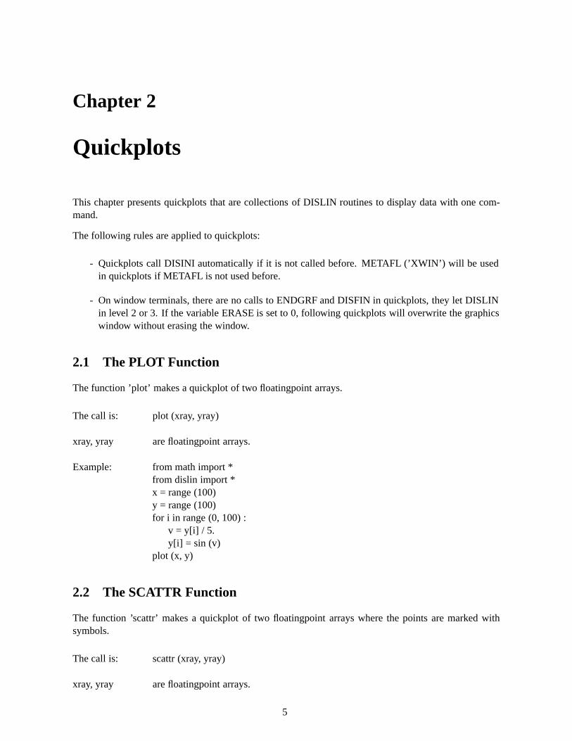
2.1 The PLOT Function

The function ’plot’ makes a quickplot of two floatingpoint arrays.

The call is: plot (xray, yray)

xray, yray are floatingpoint arrays.

Example: from math import *from dislin import *x = range (100)y = range (100)for i in range (0, 100) :

v = y[i] / 5.y[i] = sin (v)

plot (x, y)

2.2 The SCATTR Function

The function ’scattr’ makes a quickplot of two floatingpoint arrays where the points are marked withsymbols.

The call is: scattr (xray, yray)

xray, yray are floatingpoint arrays.

5

2.3 The PLOT3 Function

The function ’plot3’ makes a 3-D colour plot.

The call is: plot3 (xray, yray, zray)

xray, yray, zray are floatingpoint arrays containing X-, Y- and Z-coordinates.

2.4 The SURF3 Function

The function ’surf3’ makes a 3-D colour plot of a matrix. The columns of the matrix will be plotted asrows.

The call is: surf3 (zmat ,xray, yray)

zmat is a two-dimensional floatingpoint array with nx rows and ny columns.

xray is a floatingpoint array with the dimension nx. It will be used to position the rows ofzmat.

yray is a floatingpoint array with the dimension ny. It will be used to position the columnsof zmat.

2.5 The SURFACE Function

The function ’surface’ makes a surface plot of a matrix.

The call is: surface (zmat, xray, yray)




2.6 The SURSHADE Function

The function ’surshade’ makes a shaded surface plot of a matrix.

The call is: surshade (zmat, xray, yray)




2.7 The CONTOUR Function

The function ’contour’ makes a contour plot of a matrix.

The call is: contour (zmat, xray, yray [,zlvray])


6



zlvray is a floatingpoint array containing the levels. If zlvray is missing, 10 levels betweenthe minimum and maximum of zmat will be generated.

2.8 The CONSHADE Function

The function ’conshade’ makes a shaded contour plot of a matrix.

The call is: conshade (zmat, xray, yray [,zlvray])




zlvray is a floatingpoint array containing the levels. If zlvray is missing, 10 levels betweenthe minimum and maximum of zmat will be generated.

2.9 Scaling of Quickplots

Normally, quickplots are scaled automatically in the range of the data. This behaviour can be changed ifcertain variables are defined.

The variables for the X-axis are:

a) If the variables XMIN and XMAX are defined, the X-axis will be scaled automati-cally in the range XMIN, XMAX.

b) If the variables XMIN, XMAX, XOR and XSTEP are defined, the scaling and label-ing of the X-axis is completly defined by the user.

c) If the variable XAUTO is defined and set to 1, the variables XMIN, XMAX, XORand XSTEP will be ignored and scaling will be done automatically in the range ofthe data.

Analog: Y-axis, Z-axis.

Notes: - For logarithmic scaling, the parameters must be exponents of base 10.

- Scaling variables can be defined with the function ’setvar (cname, value)’ wherecname is a string containing the name of the variable and value a numeric value.

Example: from Numeric import *from dislin import *setvar (’YMIN’, -0.8)setvar (’YMAX’, 0.8)x = arange (100, typecode = Float32)plot (x, sin(x/5))

7

2.10 Quickplot Variables

There is a set of variables that can modify the appearance of quickplots. They can be defined with thefunction setvar that has the syntax setvar (cname, value) where cname is a string containing the name ofthe variable and value is a numeric value or a string. The following table shows all quickplot variables.The corresponding DISLIN routines are given in parenthesis.

X defines the X-axis title (NAME).

Y defines the Y-axis title (NAME).

Z defines the Z-axis title (NAME).

T1 defines line 1 of the axis system title (TITLIN).




XTIC sets the number of ticks for the X-axis (TICKS).

YTIC sets the number of ticks for the Y-axis (TICKS).

ZTIC sets the number of ticks for the Z-axis (TICKS).

XDIG sets the number of digits for the X-axis (DIGITS).

YDIG sets the number of digits for the Y-axis (DIGITS).

ZDIG sets the number of digits for the Z-axis (DIGITS).

XSCL defines the scaling of the X-axis (SCALE).

YSCL defines the scaling of the Y-axis (SCALE).

ZSCL defines the scaling of the Z-axis (SCALE).

XLAB defines the labels of the X-axis (LABELS).

YLAB defines the labels of the Y-axis (LABELS).

ZLAB defines the labels of the Z-axis (LABELS).

H defines the character size (HEIGHT).

HNAME defines the size of axis titles (HNAME).

HTITLE defines the size of the axis sytem title (HTITLE).

XPOS defines the X-position of the axis system (AXSPOS).

YPOS defines the Y-position of the axis system (AXSPOS).

XLEN defines the size of an axis system in X-direction (AXSLEN).

YLEN defines the size of an axis system in Y-direction (AXSLEN).

ZLEN defines the size of an axis system in Z-direction (AX3LEN).

POLCRV defines an interpolation method used by CURVE (POLCRV).

INCMRK defines line or symbol mode for CURVE (INCMRK).

MARKER selctes a symbol for CURVE (MARKER).

HSYMBL defines the size of symbols (HSYMBL).

8

XRES sets the width of points plotted by PLOT3 (SETRES).

YRES sets the height of points plotted by PLOT3 (SETRES).

X3VIEW sets the X-position of the viewpoint in absolut 3-D coordinates (VIEW3D).

Y3VIEW sets the Y-position of the viewpoint in absolut 3-D coordinates (VIEW3D).

Z3VIEW sets the Z-position of the viewpoint in absolut 3-D coordinates (VIEW3D).

X3LEN defines the X-axis length of the 3-D box (AXIS3D).

Y3LEN defines the Y-axis length of the 3-D box (AXIS3D).

Z3LEN defines the Z-axis length of the 3-D box (AXIS3D).

VTITLE defines vertical shifting for the axis system title (VKYTIT).

CONSHD selects an algorithm used for contour filling (SHDMOD).

Note: The variables can also be used, to initalize plotting parameters in DISINI.

Example: from Numeric import *from dislin import *setvar (’X’, ’X-axis’)setvar (’Y’, ’Y-axis’)xray = arange (10, typecode = Float32)plot (xray, xray)

9

10

Appendix A

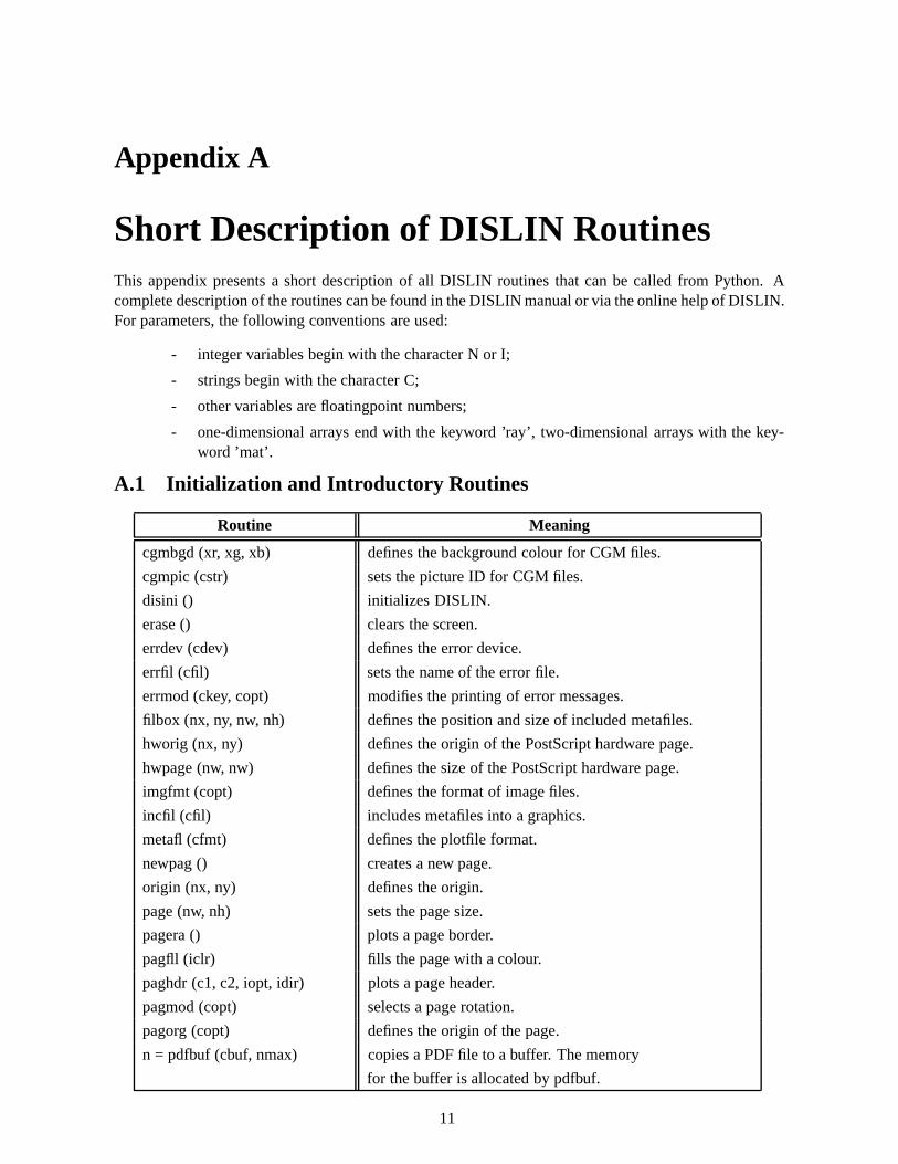
Short Description of DISLIN RoutinesThis appendix presents a short description of all DISLIN routines that can be called from Python. Acomplete description of the routines can be found in the DISLIN manual or via the online help of DISLIN.For parameters, the following conventions are used:

- integer variables begin with the character N or I;

- strings begin with the character C;

- other variables are floatingpoint numbers;

- one-dimensional arrays end with the keyword ’ray’, two-dimensional arrays with the key-word ’mat’.

A.1 Initialization and Introductory Routines

Routine Meaning

cgmbgd (xr, xg, xb) defines the background colour for CGM files.

cgmpic (cstr) sets the picture ID for CGM files.

disini () initializes DISLIN.

erase () clears the screen.

errdev (cdev) defines the error device.

errfil (cfil) sets the name of the error file.

errmod (ckey, copt) modifies the printing of error messages.

filbox (nx, ny, nw, nh) defines the position and size of included metafiles.

hworig (nx, ny) defines the origin of the PostScript hardware page.

hwpage (nw, nw) defines the size of the PostScript hardware page.

imgfmt (copt) defines the format of image files.

incfil (cfil) includes metafiles into a graphics.

metafl (cfmt) defines the plotfile format.

newpag () creates a new page.

origin (nx, ny) defines the origin.

page (nw, nh) sets the page size.

pagera () plots a page border.

pagfll (iclr) fills the page with a colour.

paghdr (c1, c2, iopt, idir) plots a page header.

pagmod (copt) selects a page rotation.

pagorg (copt) defines the origin of the page.

n = pdfbuf (cbuf, nmax) copies a PDF file to a buffer. The memory

for the buffer is allocated by pdfbuf.

11

Routine Meaning

pdfmod (cmod, ckey) defines PDF options.

pngmod (cmod, ckey) enables transparency for PNG files.

sclfac (x) defines a scaling factor for the entire plot.

sclmod (copt) defines a scaling mode.

scrmod (copt) swaps back- and foreground colours.

setfil (cfil) sets the plotfile name.

setpag (copt) selects a predefined page format.

setxid (id, copt) defines an external X Window or pixmap.

symfil (cdev, cstat) sends a plotfile to a device.

tifmod (n, cval, copt) defines the physical resolution of TIFF files.

unit (nu) defines the logical unit for messages.

units (copt) defines the plot units.

wmfmod (cmod, ckey) modifies the format of WMF files.

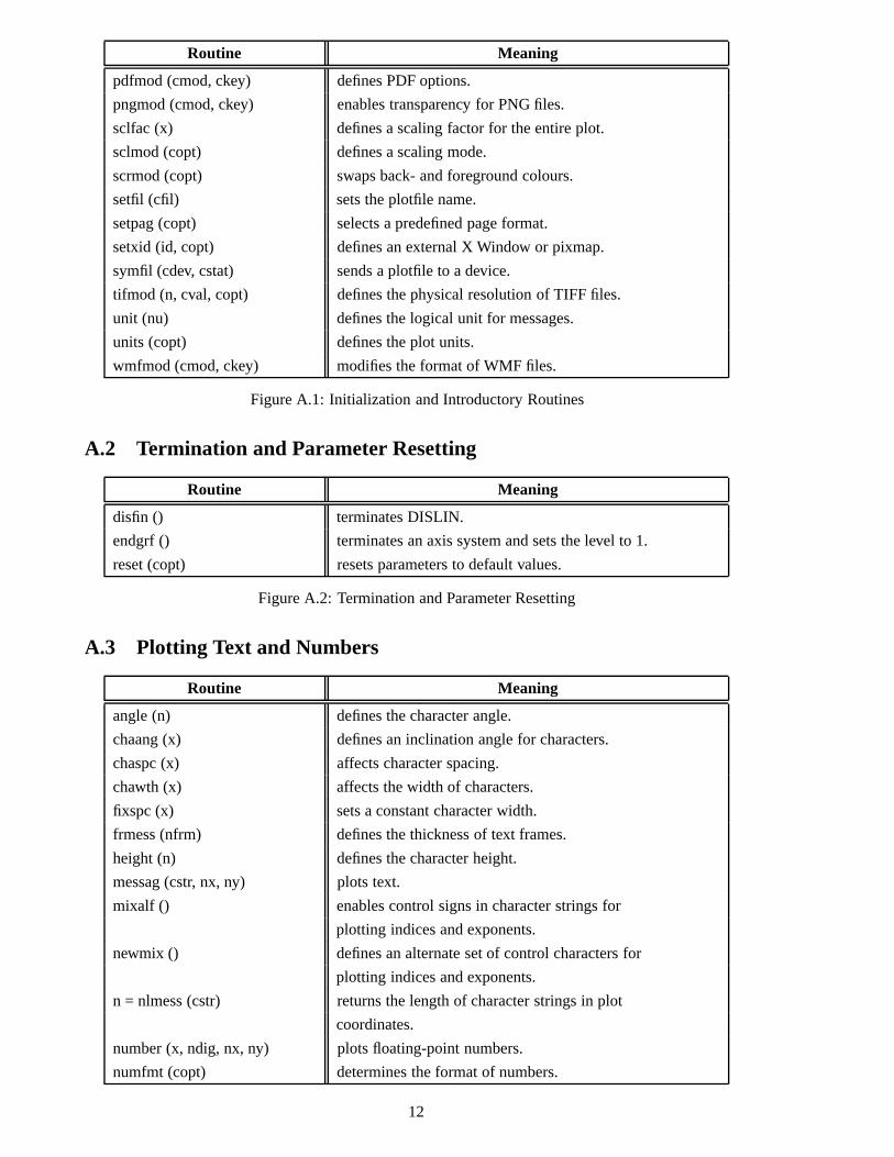
Figure A.1: Initialization and Introductory Routines

A.2 Termination and Parameter Resetting

Routine Meaning

disfin () terminates DISLIN.

endgrf () terminates an axis system and sets the level to 1.

reset (copt) resets parameters to default values.

Figure A.2: Termination and Parameter Resetting

A.3 Plotting Text and Numbers

Routine Meaning

angle (n) defines the character angle.

chaang (x) defines an inclination angle for characters.

chaspc (x) affects character spacing.

chawth (x) affects the width of characters.

fixspc (x) sets a constant character width.

frmess (nfrm) defines the thickness of text frames.

height (n) defines the character height.

messag (cstr, nx, ny) plots text.

mixalf () enables control signs in character strings for

plotting indices and exponents.

newmix () defines an alternate set of control characters for

plotting indices and exponents.

n = nlmess (cstr) returns the length of character strings in plot

coordinates.

number (x, ndig, nx, ny) plots floating-point numbers.

numfmt (copt) determines the format of numbers.

12

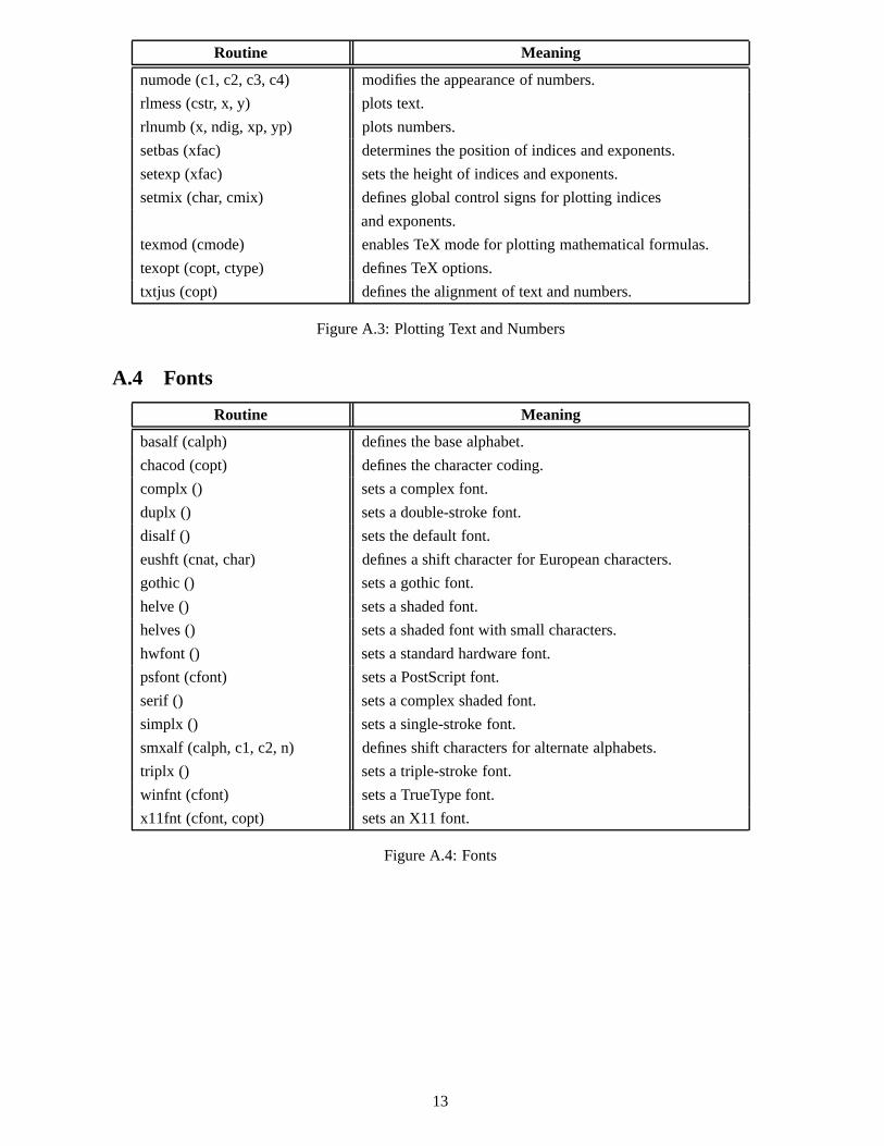
Routine Meaning

numode (c1, c2, c3, c4) modifies the appearance of numbers.

rlmess (cstr, x, y) plots text.

rlnumb (x, ndig, xp, yp) plots numbers.

setbas (xfac) determines the position of indices and exponents.

setexp (xfac) sets the height of indices and exponents.

setmix (char, cmix) defines global control signs for plotting indices

and exponents.

texmod (cmode) enables TeX mode for plotting mathematical formulas.

texopt (copt, ctype) defines TeX options.

txtjus (copt) defines the alignment of text and numbers.

Figure A.3: Plotting Text and Numbers

A.4 Fonts

Routine Meaning

basalf (calph) defines the base alphabet.

chacod (copt) defines the character coding.

complx () sets a complex font.

duplx () sets a double-stroke font.

disalf () sets the default font.

eushft (cnat, char) defines a shift character for European characters.

gothic () sets a gothic font.

helve () sets a shaded font.

helves () sets a shaded font with small characters.

hwfont () sets a standard hardware font.

psfont (cfont) sets a PostScript font.

serif () sets a complex shaded font.

simplx () sets a single-stroke font.

smxalf (calph, c1, c2, n) defines shift characters for alternate alphabets.

triplx () sets a triple-stroke font.

winfnt (cfont) sets a TrueType font.

x11fnt (cfont, copt) sets an X11 font.

Figure A.4: Fonts

13

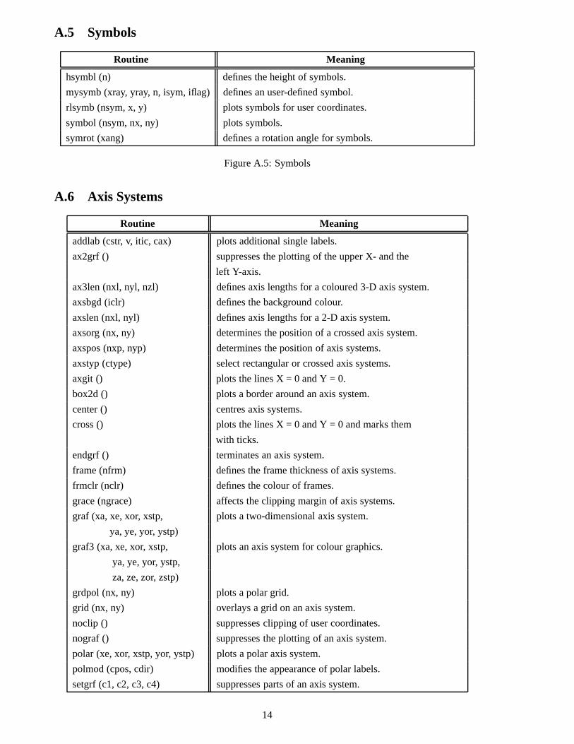
A.5 Symbols

Routine Meaning

hsymbl (n) defines the height of symbols.

mysymb (xray, yray, n, isym, iflag) defines an user-defined symbol.

rlsymb (nsym, x, y) plots symbols for user coordinates.

symbol (nsym, nx, ny) plots symbols.

symrot (xang) defines a rotation angle for symbols.

Figure A.5: Symbols

A.6 Axis Systems

Routine Meaning

addlab (cstr, v, itic, cax) plots additional single labels.

ax2grf () suppresses the plotting of the upper X- and the

left Y-axis.

ax3len (nxl, nyl, nzl) defines axis lengths for a coloured 3-D axis system.

axsbgd (iclr) defines the background colour.

axslen (nxl, nyl) defines axis lengths for a 2-D axis system.

axsorg (nx, ny) determines the position of a crossed axis system.

axspos (nxp, nyp) determines the position of axis systems.

axstyp (ctype) select rectangular or crossed axis systems.

axgit () plots the lines X = 0 and Y = 0.

box2d () plots a border around an axis system.

center () centres axis systems.

cross () plots the lines X = 0 andY = 0 and marks them

with ticks.

endgrf () terminates an axis system.

frame (nfrm) defines the frame thickness of axis systems.

frmclr (nclr) defines the colour of frames.

grace (ngrace) affects the clipping margin of axis systems.

graf (xa, xe, xor, xstp, plots a two-dimensional axis system.

ya, ye, yor, ystp)

graf3 (xa, xe, xor, xstp, plots an axis system for colour graphics.

ya, ye, yor, ystp,

za, ze, zor, zstp)

grdpol (nx, ny) plots a polar grid.

grid (nx, ny) overlays a grid on an axis system.

noclip () suppresses clipping of user coordinates.

nograf () suppresses the plotting of an axis system.

polar (xe, xor, xstp, yor, ystp) plots a polar axis system.

polmod (cpos, cdir) modifies the appearance of polar labels.

setgrf (c1, c2, c3, c4) suppresses parts of an axis system.

14

Routine Meaning

setscl (xray, n, cax) sets automatic scaling.

title () plots a title over an axis system.

xaxgit () plots the line Y = 0.

xcross () plots the line Y = 0 and marks it with ticks.

yaxgit () plots the line X = 0.

ycross () plots the line X = 0 and marks it with ticks.

Figure A.6: Axis Systems

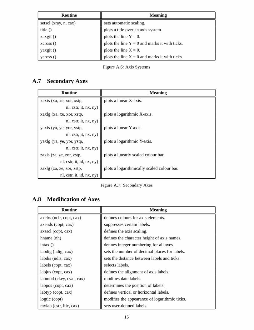
A.7 Secondary Axes

Routine Meaning

xaxis (xa, xe, xor, xstp, plots a linear X-axis.

nl, cstr, it, nx, ny)

xaxlg (xa, xe, xor, xstp, plots a logarithmic X-axis.


yaxis (ya, ye, yor, ystp, plots a linear Y-axis.


yaxlg (ya, ye, yor, ystp, plots a logarithmic Y-axis.


zaxis (za, ze, zor, zstp, plots a linearly scaled colour bar.

nl, cstr, it, id, nx, ny)

zaxlg (za, ze, zor, zstp, plots a logarithmically scaled colour bar.


Figure A.7: Secondary Axes

A.8 Modification of Axes

Routine Meaning

axclrs (nclr, copt, cax) defines colours for axis elements.

axends (copt, cax) suppresses certain labels.

axsscl (copt, cax) defines the axis scaling.

hname (nh) defines the character height of axis names.

intax () defines integer numbering for all axes.

labdig (ndig, cax) sets the number of decimal places for labels.

labdis (ndis, cax) sets the distance between labels and ticks.

labels (copt, cax) selects labels.

labjus (copt, cax) defines the alignment of axis labels.

labmod (ckey, cval, cax) modifies date labels.

labpos (copt, cax) determines the position of labels.

labtyp (copt, cax) defines vertical or horizontal labels.

logtic (copt) modifies the appearance of logarithmic ticks.

mylab (cstr, itic, cax) sets user-defined labels.

15

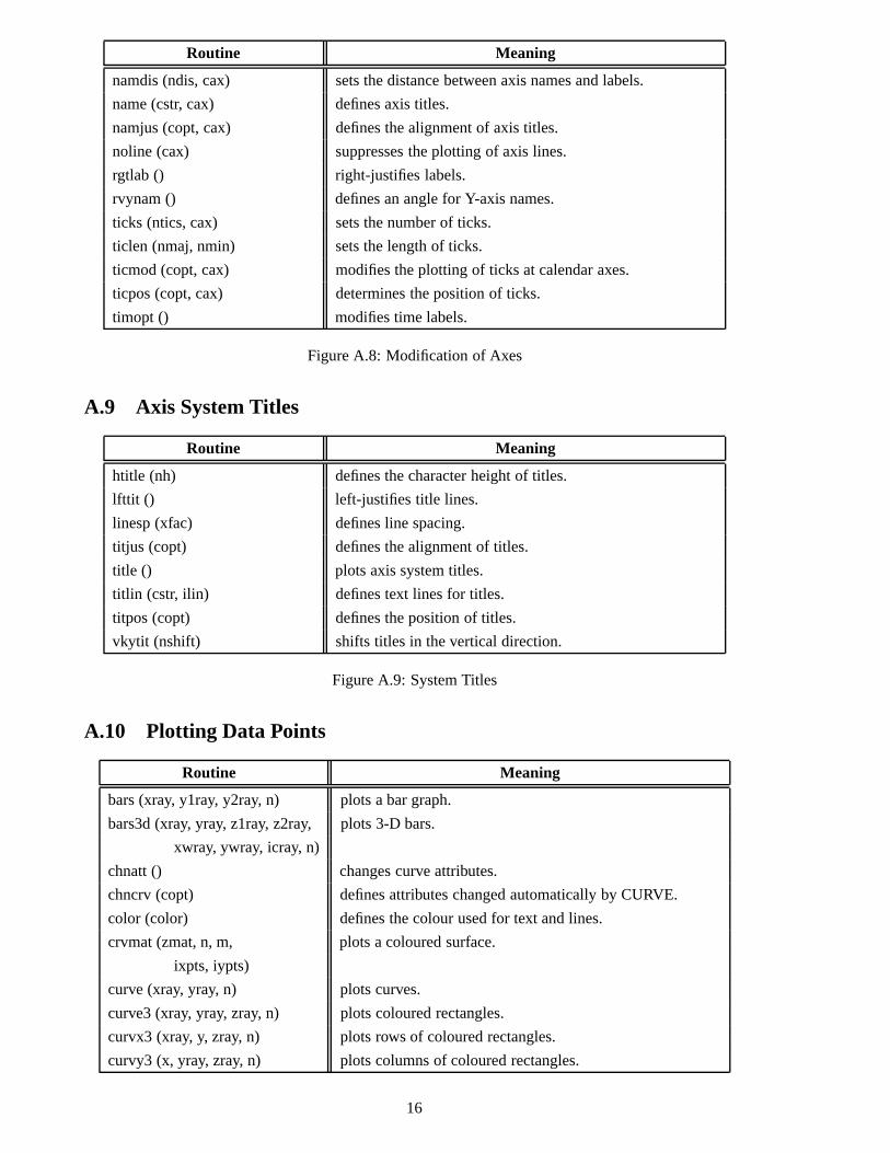
Routine Meaning

namdis (ndis, cax) sets the distance between axis names and labels.

name (cstr, cax) defines axis titles.

namjus (copt, cax) defines the alignment of axis titles.

noline (cax) suppresses the plotting of axis lines.

rgtlab () right-justifies labels.

rvynam () defines an angle for Y-axis names.

ticks (ntics, cax) sets the number of ticks.

ticlen (nmaj, nmin) sets the length of ticks.

ticmod (copt, cax) modifies the plotting of ticks at calendar axes.

ticpos (copt, cax) determines the position of ticks.

timopt () modifies time labels.

Figure A.8: Modification of Axes

A.9 Axis System Titles

Routine Meaning

htitle (nh) defines the character height of titles.

lfttit () left-justifies title lines.

linesp (xfac) defines line spacing.

titjus (copt) defines the alignment of titles.

title () plots axis system titles.

titlin (cstr, ilin) defines text lines for titles.

titpos (copt) defines the position of titles.

vkytit (nshift) shifts titles in the vertical direction.

Figure A.9: System Titles

A.10 Plotting Data Points

Routine Meaning

bars (xray, y1ray, y2ray, n) plots a bar graph.

bars3d (xray, yray, z1ray, z2ray, plots 3-D bars.

xwray, ywray, icray, n)

chnatt () changes curve attributes.

chncrv (copt) defines attributes changed automatically by CURVE.

color (color) defines the colour used for text and lines.

crvmat (zmat, n, m, plots a coloured surface.

ixpts, iypts)

curve (xray, yray, n) plots curves.

curve3 (xray, yray, zray, n) plots coloured rectangles.

curvx3 (xray, y, zray, n) plots rows of coloured rectangles.

curvy3 (x, yray, zray, n) plots columns of coloured rectangles.

16

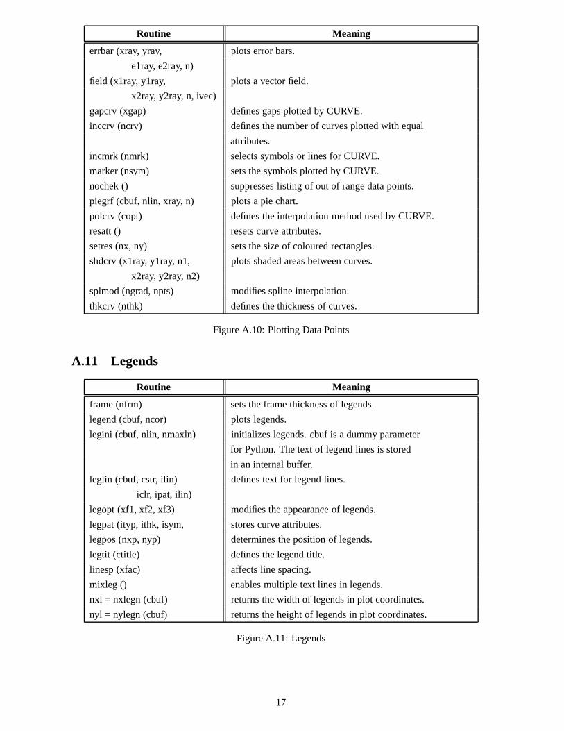
Routine Meaning

errbar (xray, yray, plots error bars.

e1ray, e2ray, n)

field (x1ray, y1ray, plots a vector field.

x2ray, y2ray, n, ivec)

gapcrv (xgap) defines gaps plotted by CURVE.

inccrv (ncrv) defines the number of curves plotted with equal

attributes.

incmrk (nmrk) selects symbols or lines for CURVE.

marker (nsym) sets the symbols plotted by CURVE.

nochek () suppresses listing of out of range data points.

piegrf (cbuf, nlin, xray, n) plots a pie chart.

polcrv (copt) defines the interpolation method used by CURVE.

resatt () resets curve attributes.

setres (nx, ny) sets the size of coloured rectangles.

shdcrv (x1ray, y1ray, n1, plots shaded areas between curves.

x2ray, y2ray, n2)

splmod (ngrad, npts) modifies spline interpolation.

thkcrv (nthk) defines the thickness of curves.

Figure A.10: Plotting Data Points

A.11 Legends

Routine Meaning

frame (nfrm) sets the frame thickness of legends.

legend (cbuf, ncor) plots legends.

legini (cbuf, nlin, nmaxln) initializes legends. cbuf is a dummy parameter

for Python. The text of legend lines is stored

in an internal buffer.

leglin (cbuf, cstr, ilin) defines text for legend lines.

iclr, ipat, ilin)

legopt (xf1, xf2, xf3) modifies the appearance of legends.

legpat (ityp, ithk, isym, stores curve attributes.

legpos (nxp, nyp) determines the position of legends.

legtit (ctitle) defines the legend title.

linesp (xfac) affects line spacing.

mixleg () enables multiple text lines in legends.

nxl = nxlegn (cbuf) returns the width of legends in plot coordinates.

nyl = nylegn (cbuf) returns the height of legends in plot coordinates.

Figure A.11: Legends

17

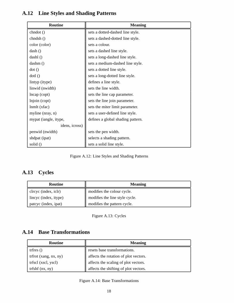
A.12 Line Styles and Shading Patterns

Routine Meaning

chndot () sets a dotted-dashed line style.

chndsh () sets a dashed-dotted line style.

color (color) sets a colour.

dash () sets a dashed line style.

dashl () sets a long-dashed line style.

dashm () sets a medium-dashed line style.

dot () sets a dotted line style.

dotl () sets a long-dotted line style.

lintyp (itype) defines a line style.

linwid (nwidth) sets the line width.

lncap (copt) sets the line cap parameter.

lnjoin (copt) sets the line join parameter.

lnmlt (xfac) sets the miter limit parameter.

myline (nray, n) sets a user-defined line style.

mypat (iangle, itype, defines a global shading pattern.

idens, icross)

penwid (nwidth) sets the pen width.

shdpat (ipat) selects a shading pattern.

solid () sets a solid line style.

Figure A.12: Line Styles and Shading Patterns

A.13 Cycles

Routine Meaning

clrcyc (index, iclr) modifies the colour cycle.

lincyc (index, itype) modifies the line style cycle.

patcyc (index, ipat) modifies the pattern cycle.

Figure A.13: Cycles

A.14 Base Transformations

Routine Meaning

trfres () resets base transformations.

trfrot (xang, nx, ny) affects the rotation of plot vectors.

trfscl (xscl, yscl) affects the scaling of plot vectors.

trfshf (nx, ny) affects the shifting of plot vectors.

Figure A.14: Base Transformations

18

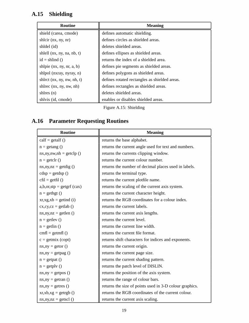
A.15 Shielding

Routine Meaning

shield (carea, cmode) defines automatic shielding.

shlcir (nx, ny, nr) defines circles as shielded areas.

shldel (id) deletes shielded areas.

shlell (nx, ny, na, nb, t) defines ellipses as shielded areas.

id = shlind () returns the index of a shielded area.

shlpie (nx, ny, nr, a, b) defines pie segments as shielded areas.

shlpol (nxray, nyray, n) defines polygons as shielded areas.

shlrct (nx, ny, nw, nh, t) defines rotated rectangles as shielded areas.

shlrec (nx, ny, nw, nh) defines rectangles as shielded areas.

shlres (n) deletes shielded areas.

shlvis (id, cmode) enables or disables shielded areas.

Figure A.15: Shielding

A.16 Parameter Requesting Routines

Routine Meaning

calf = getalf () returns the base alphabet.

n = getang () returns the current angle used for text and numbers.

nx,ny,nw,nh = getclp () returns the currents clipping window.

n = getclr () returns the current colour number.

nx,ny,nz = getdig () returns the number of decimal places used in labels.

cdsp = getdsp () returns the terminal type.

cfil = getfil () returns the current plotfile name.

a,b,or,stp = getgrf (cax) returns the scaling of the current axis system.

n = gethgt () returns the current character height.

xr,xg,xb = getind (i) returns the RGB coordinates for a colour index.

cx,cy,cz = getlab () returns the current labels.

nx,ny,nz = getlen () returns the current axis lengths.

n = getlev () returns the current level.

n = getlin () returns the current line width.

cmfl = getmfl () returns the current file format.

c = getmix (copt) returns shift characters for indices and exponents.

nx,ny = getor () returns the current origin.

nx,ny = getpag () returns the current page size.

n = getpat () returns the current shading pattern.

n = getplv () returns the patch level of DISLIN.

nx,ny = getpos () returns the position of the axis system.

nx,ny = getran () returns the range of colour bars.

nx,ny = getres () returns the size of points used in 3-D colour graphics.

xr,xb,xg = getrgb () returns the RGB coordinates of the current colour.

nx,ny,nz = getscl () returns the current axis scaling.

19

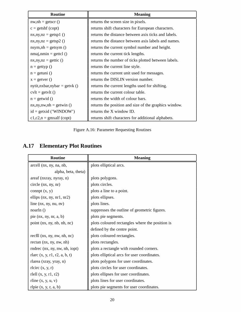
Routine Meaning

nw,nh = getscr () returns the screen size in pixels.

c = getshf (copt) returns shift characters for European characters.

nx,ny,nz = getsp1 () returns the distance between axis ticks and labels.

nx,ny,nz = getsp2 () returns the distance between axis labels and names.

nsym,nh = getsym () returns the current symbol number and height.

nmaj,nmin = gettcl () returns the current tick lengths.

nx,ny,nz = gettic () returns the number of ticks plotted between labels.

n = gettyp () returns the current line style.

n = getuni () returns the current unit used for messages.

x = getver () returns the DISLIN version number.

nytit,nxbar,nybar = getvk () returns the current lengths used for shifting.

cvlt = getvlt () returns the current colour table.

n = getwid () returns the width of colour bars.

nx,ny,nw,nh = getwin () returns the position and size of the graphics window.

id = getxid (’WINDOW’) returns the X window ID.

c1,c2,n = gmxalf (copt) returns shift characters for additional alphabets.

Figure A.16: Parameter Requesting Routines

A.17 Elementary Plot Routines

Routine Meaning

arcell (nx, ny, na, nb, plots elliptical arcs.

alpha, beta, theta)

areaf (nxray, nyray, n) plots polygons.

circle (nx, ny, nr) plots circles.

connpt (x, y) plots a line to a point.

ellips (nx, ny, nr1, nr2) plots ellipses.

line (nx, ny, nu, nv) plots lines.

noarln () suppresses the outline of geometric figures.

pie (nx, ny, nr, a, b) plots pie segments.

point (nx, ny, nb, nh, nc) plots coloured rectangles where the position is

defined by the centre point.

recfll (nx, ny, nw, nh, nc) plots coloured rectangles.

rectan (nx, ny, nw, nh) plots rectangles.

rndrec (nx, ny, nw, nh, iopt) plots a rectangle with rounded corners.

rlarc (x, y, r1, r2, a, b, t) plots elliptical arcs for user coordinates.

rlarea (xray, yray, n) plots polygons for user coordinates.

rlcirc (x, y, r) plots circles for user coordinates.

rlell (x, y, r1, r2) plots ellipses for user coordinates.

rline (x, y, u, v) plots lines for user coordinates.

rlpie (x, y, r, a, b) plots pie segments for user coordinates.

20

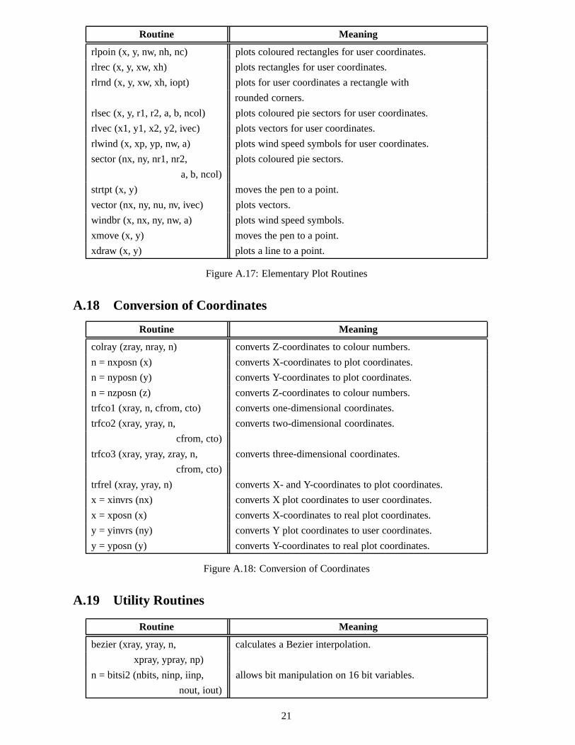
Routine Meaning

rlpoin (x, y, nw, nh, nc) plots coloured rectangles for user coordinates.

rlrec (x, y, xw, xh) plots rectangles for user coordinates.

rlrnd (x, y, xw, xh, iopt) plots for user coordinates a rectangle with

rounded corners.

rlsec (x, y, r1, r2, a, b, ncol) plots coloured pie sectors for user coordinates.

rlvec (x1, y1, x2, y2, ivec) plots vectors for user coordinates.

rlwind (x, xp, yp, nw, a) plots wind speed symbols for user coordinates.

sector (nx, ny, nr1, nr2, plots coloured pie sectors.

a, b, ncol)

strtpt (x, y) moves the pen to a point.

vector (nx, ny, nu, nv, ivec) plots vectors.

windbr (x, nx, ny, nw, a) plots wind speed symbols.

xmove (x, y) moves the pen to a point.

xdraw (x, y) plots a line to a point.

Figure A.17: Elementary Plot Routines

A.18 Conversion of Coordinates

Routine Meaning

colray (zray, nray, n) converts Z-coordinates to colour numbers.

n = nxposn (x) converts X-coordinates to plot coordinates.

n = nyposn (y) converts Y-coordinates to plot coordinates.

n = nzposn (z) converts Z-coordinates to colour numbers.

trfco1 (xray, n, cfrom, cto) converts one-dimensional coordinates.

trfco2 (xray, yray, n, converts two-dimensional coordinates.

cfrom, cto)

trfco3 (xray, yray, zray, n, converts three-dimensional coordinates.

cfrom, cto)

trfrel (xray, yray, n) converts X- and Y-coordinates to plot coordinates.

x = xinvrs (nx) converts X plot coordinates to user coordinates.

x = xposn (x) converts X-coordinates to real plot coordinates.

y = yinvrs (ny) converts Y plot coordinates to user coordinates.

y = yposn (y) converts Y-coordinates to real plot coordinates.

Figure A.18: Conversion of Coordinates

A.19 Utility Routines

Routine Meaning

bezier (xray, yray, n, calculates a Bezier interpolation.

xpray, ypray, np)

n = bitsi2 (nbits, ninp, iinp, allows bit manipulation on 16 bit variables.

nout, iout)

21

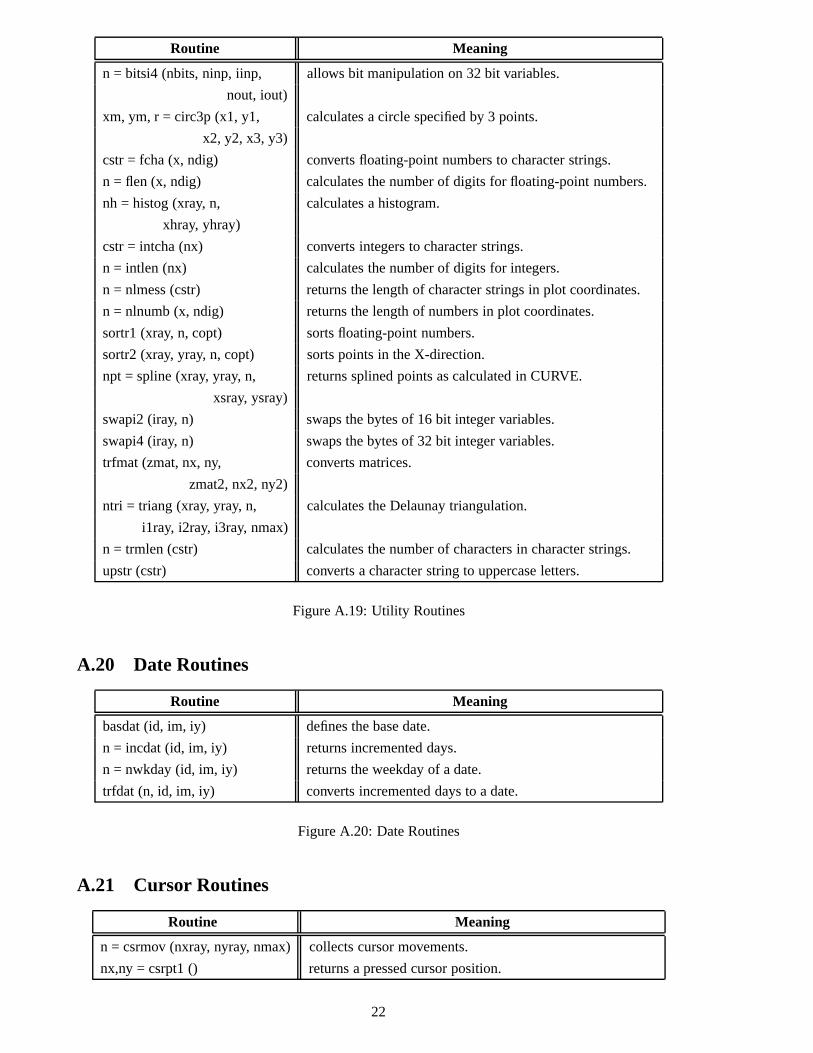
Routine Meaning

n = bitsi4 (nbits, ninp, iinp, allows bit manipulation on 32 bit variables.

nout, iout)

xm, ym, r = circ3p (x1, y1, calculates a circle specified by 3 points.

x2, y2, x3, y3)

cstr = fcha (x, ndig) converts floating-point numbers to character strings.

n = flen (x, ndig) calculates the number of digits for floating-point numbers.

nh = histog (xray, n, calculates a histogram.

xhray, yhray)

cstr = intcha (nx) converts integers to character strings.

n = intlen (nx) calculates the number of digits for integers.

n = nlmess (cstr) returns the length of character strings in plot coordinates.

n = nlnumb (x, ndig) returns the length of numbers in plot coordinates.

sortr1 (xray, n, copt) sorts floating-point numbers.

sortr2 (xray, yray, n, copt) sorts points in the X-direction.

npt = spline (xray, yray, n, returns splined points as calculated in CURVE.

xsray, ysray)

swapi2 (iray, n) swaps the bytes of 16 bit integer variables.

swapi4 (iray, n) swaps the bytes of 32 bit integer variables.

trfmat (zmat, nx, ny, converts matrices.

zmat2, nx2, ny2)

ntri = triang (xray, yray, n, calculates the Delaunay triangulation.

i1ray, i2ray, i3ray, nmax)

n = trmlen (cstr) calculates the number of characters in character strings.

upstr (cstr) converts a character string to uppercase letters.

Figure A.19: Utility Routines

A.20 Date Routines

Routine Meaning

basdat (id, im, iy) defines the base date.

n = incdat (id, im, iy) returns incremented days.

n = nwkday (id, im, iy) returns the weekday of a date.

trfdat (n, id, im, iy) converts incremented days to a date.

Figure A.20: Date Routines

A.21 Cursor Routines

Routine Meaning

n = csrmov (nxray, nyray, nmax) collects cursor movements.

nx,ny = csrpt1 () returns a pressed cursor position.

22

Routine Meaning

n = csrpts (nxray, nyray, nmax) collects cursor positions.

csruni (copt) selects the unit of returned cursor positions.

Figure A.21: Cursor Routines

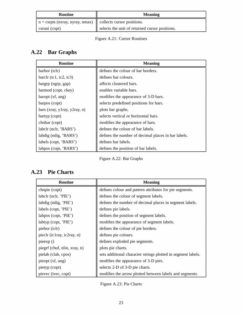
A.22 Bar Graphs

Routine Meaning

barbor (iclr) defines the colour of bar borders.

barclr (ic1, ic2, ic3) defines bar colours.

bargrp (ngrp, gap) affects clustered bars.

barmod (copt, ckey) enables variable bars.

baropt (xf, ang) modifies the appearance of 3-D bars.

barpos (copt) selects predefined positions for bars.

bars (xray, y1ray, y2ray, n) plots bar graphs.

bartyp (copt) selects vertical or horizontal bars.

chnbar (copt) modifies the appearance of bars.

labclr (nclr, ’BARS’) defines the colour of bar labels.

labdig (ndig, ’BARS’) defines the number of decimal places in bar labels.

labels (copt, ’BARS’) defines bar labels.

labpos (copt, ’BARS’) defines the position of bar labels.

Figure A.22: Bar Graphs

A.23 Pie Charts

Routine Meaning

chnpie (copt) defines colour and pattern attributes for pie segments.

labclr (nclr, ’PIE’) defines the colour of segment labels.

labdig (ndig, ’PIE’) defines the number of decimal places in segment labels.

labels (copt, ’PIE’) defines pie labels.

labpos (copt, ’PIE’) defines the position of segment labels.

labtyp (copt, ’PIE’) modifies the appearance of segment labels.

piebor (iclr) defines the colour of pie borders.

pieclr (ic1ray, ic2ray, n) defines pie colours.

pieexp () defines exploded pie segments.

piegrf (cbuf, nlin, xray, n) plots pie charts.

pielab (clab, cpos) sets additional character strings plotted in segment labels.

pieopt (xf, ang) modifies the appearance of 3-D pies.

pietyp (copt) selects 2-D of 3-D pie charts.

pievec (ivec, copt) modifies the arrow plotted between labels and segments.

Figure A.23: Pie Charts

23

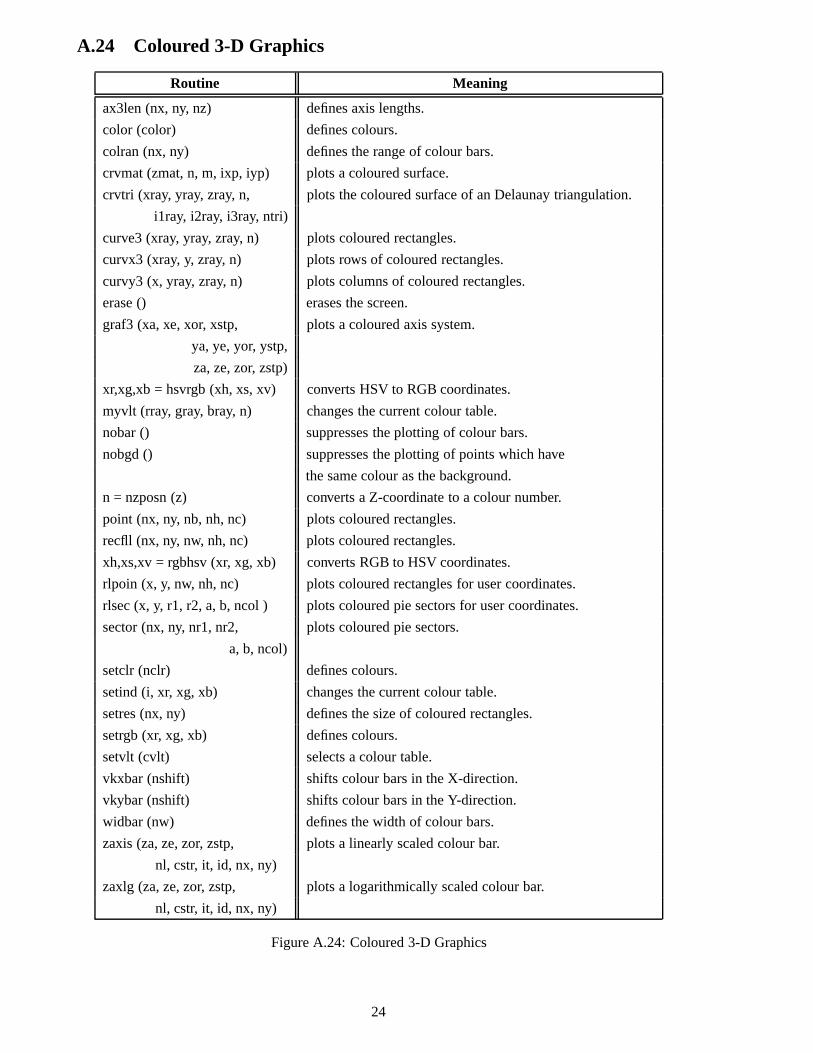
A.24 Coloured 3-D Graphics

Routine Meaning

ax3len (nx, ny, nz) defines axis lengths.

color (color) defines colours.

colran (nx, ny) defines the range of colour bars.

crvmat (zmat, n, m, ixp, iyp) plots a coloured surface.

crvtri (xray, yray, zray, n, plots the coloured surface of an Delaunay triangulation.

i1ray, i2ray, i3ray, ntri)

curve3 (xray, yray, zray, n) plots coloured rectangles.

curvx3 (xray, y, zray, n) plots rows of coloured rectangles.

curvy3 (x, yray, zray, n) plots columns of coloured rectangles.

erase () erases the screen.

graf3 (xa, xe, xor, xstp, plots a coloured axis system.

ya, ye, yor, ystp,

za, ze, zor, zstp)

xr,xg,xb = hsvrgb (xh, xs, xv) converts HSV to RGB coordinates.

myvlt (rray, gray, bray, n) changes the current colour table.

nobar () suppresses the plotting of colour bars.

nobgd () suppresses the plotting of points which have

the same colour as the background.

n = nzposn (z) converts a Z-coordinate to a colour number.

point (nx, ny, nb, nh, nc) plots coloured rectangles.

recfll (nx, ny, nw, nh, nc) plots coloured rectangles.

xh,xs,xv = rgbhsv (xr, xg, xb) converts RGB to HSV coordinates.

rlpoin (x, y, nw, nh, nc) plots coloured rectangles for user coordinates.

rlsec (x, y, r1, r2, a, b, ncol ) plots coloured pie sectors for user coordinates.

sector (nx, ny, nr1, nr2, plots coloured pie sectors.

a, b, ncol)

setclr (nclr) defines colours.

setind (i, xr, xg, xb) changes the current colour table.

setres (nx, ny) defines the size of coloured rectangles.

setrgb (xr, xg, xb) defines colours.

setvlt (cvlt) selects a colour table.

vkxbar (nshift) shifts colour bars in the X-direction.

vkybar (nshift) shifts colour bars in the Y-direction.

widbar (nw) defines the width of colour bars.

zaxis (za, ze, zor, zstp, plots a linearly scaled colour bar.


zaxlg (za, ze, zor, zstp, plots a logarithmically scaled colour bar.


Figure A.24: Coloured 3-D Graphics

24

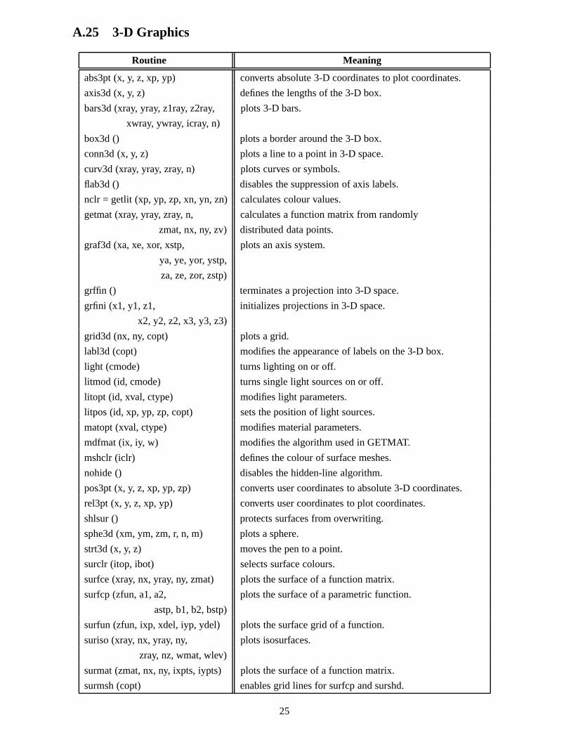
A.25 3-D Graphics

Routine Meaning

abs3pt (x, y, z, xp, yp) converts absolute 3-D coordinates to plot coordinates.

axis3d (x, y, z) defines the lengths of the 3-D box.

bars3d (xray, yray, z1ray, z2ray, plots 3-D bars.

xwray, ywray, icray, n)

box3d () plots a border around the 3-D box.

conn3d (x, y, z) plots a line to a point in 3-D space.

curv3d (xray, yray, zray, n) plots curves or symbols.

flab3d () disables the suppression of axis labels.

nclr = getlit (xp, yp, zp, xn, yn, zn) calculates colour values.

getmat (xray, yray, zray, n, calculates a function matrix from randomly

zmat, nx, ny, zv) distributed data points.

graf3d (xa, xe, xor, xstp, plots an axis system.

ya, ye, yor, ystp,

za, ze, zor, zstp)

grffin () terminates a projection into 3-D space.

grfini (x1, y1, z1, initializes projections in 3-D space.

x2, y2, z2, x3, y3, z3)

grid3d (nx, ny, copt) plots a grid.

labl3d (copt) modifies the appearance of labels on the 3-D box.

light (cmode) turns lighting on or off.

litmod (id, cmode) turns single light sources on or off.

litopt (id, xval, ctype) modifies light parameters.

litpos (id, xp, yp, zp, copt) sets the position of light sources.

matopt (xval, ctype) modifies material parameters.

mdfmat (ix, iy, w) modifies the algorithm used in GETMAT.

mshclr (iclr) defines the colour of surface meshes.

nohide () disables the hidden-line algorithm.

pos3pt (x, y, z, xp, yp, zp) converts user coordinates to absolute 3-D coordinates.

rel3pt (x, y, z, xp, yp) converts user coordinates to plot coordinates.

shlsur () protects surfaces from overwriting.

sphe3d (xm, ym, zm, r, n, m) plots a sphere.

strt3d (x, y, z) moves the pen to a point.

surclr (itop, ibot) selects surface colours.

surfce (xray, nx, yray, ny, zmat) plots the surface of a function matrix.

surfcp (zfun, a1, a2, plots the surface of a parametric function.

astp, b1, b2, bstp)

surfun (zfun, ixp, xdel, iyp, ydel) plots the surface grid of a function.

suriso (xray, nx, yray, ny, plots isosurfaces.

zray, nz, wmat, wlev)

surmat (zmat, nx, ny, ixpts, iypts) plots the surface of a function matrix.

surmsh (copt) enables grid lines for surfcp and surshd.

25

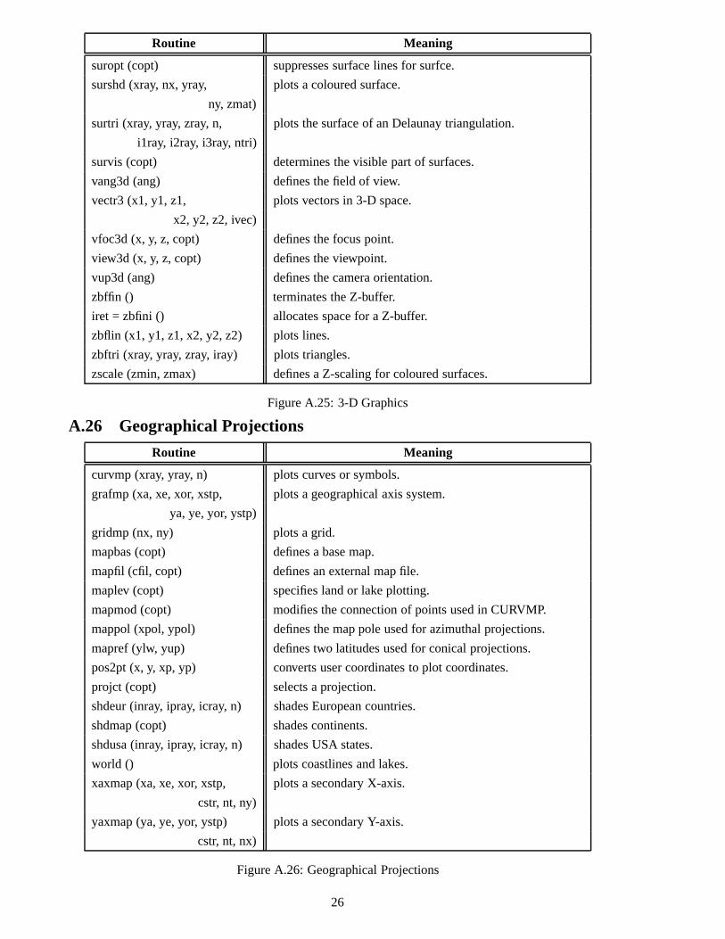
Routine Meaning

suropt (copt) suppresses surface lines for surfce.

surshd (xray, nx, yray, plots a coloured surface.

ny, zmat)

surtri (xray, yray, zray, n, plots the surface of an Delaunay triangulation.

i1ray, i2ray, i3ray, ntri)

survis (copt) determines the visible part of surfaces.

vang3d (ang) defines the field of view.

vectr3 (x1, y1, z1, plots vectors in 3-D space.

x2, y2, z2, ivec)

vfoc3d (x, y, z, copt) defines the focus point.

view3d (x, y, z, copt) defines the viewpoint.

vup3d (ang) defines the camera orientation.

zbffin () terminates the Z-buffer.

iret = zbfini () allocates space for a Z-buffer.

zbflin (x1, y1, z1, x2, y2, z2) plots lines.

zbftri (xray, yray, zray, iray) plots triangles.

zscale (zmin, zmax) defines a Z-scaling for coloured surfaces.

Figure A.25: 3-D Graphics

A.26 Geographical Projections

Routine Meaning

curvmp (xray, yray, n) plots curves or symbols.

grafmp (xa, xe, xor, xstp, plots a geographical axis system.

ya, ye, yor, ystp)

gridmp (nx, ny) plots a grid.

mapbas (copt) defines a base map.

mapfil (cfil, copt) defines an external map file.

maplev (copt) specifies land or lake plotting.

mapmod (copt) modifies the connection of points used in CURVMP.

mappol (xpol, ypol) defines the map pole used for azimuthal projections.

mapref (ylw, yup) defines two latitudes used for conical projections.

pos2pt (x, y, xp, yp) converts user coordinates to plot coordinates.

projct (copt) selects a projection.

shdeur (inray, ipray, icray, n) shades European countries.

shdmap (copt) shades continents.

shdusa (inray, ipray, icray, n) shades USA states.

world () plots coastlines and lakes.

xaxmap (xa, xe, xor, xstp, plots a secondary X-axis.

cstr, nt, ny)

yaxmap (ya, ye, yor, ystp) plots a secondary Y-axis.

cstr, nt, nx)

Figure A.26: Geographical Projections

26

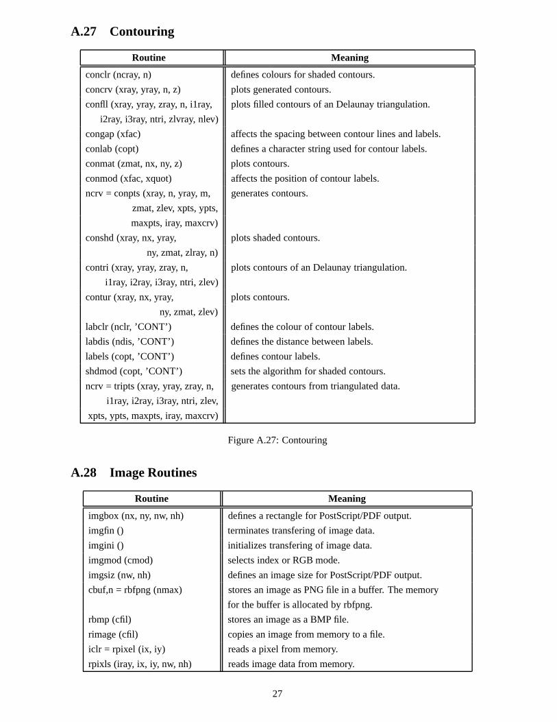
A.27 Contouring

Routine Meaning

conclr (ncray, n) defines colours for shaded contours.

concrv (xray, yray, n, z) plots generated contours.

confll (xray, yray, zray, n, i1ray, plots filled contours of an Delaunay triangulation.

i2ray, i3ray, ntri, zlvray, nlev)

congap (xfac) affects the spacing between contour lines and labels.

conlab (copt) defines a character string used for contour labels.

conmat (zmat, nx, ny, z) plots contours.

conmod (xfac, xquot) affects the position of contour labels.

ncrv = conpts (xray, n, yray, m, generates contours.

zmat, zlev, xpts, ypts,

maxpts, iray, maxcrv)

conshd (xray, nx, yray, plots shaded contours.

ny, zmat, zlray, n)

contri (xray, yray, zray, n, plots contours of an Delaunay triangulation.

i1ray, i2ray, i3ray, ntri, zlev)

contur (xray, nx, yray, plots contours.

ny, zmat, zlev)

labclr (nclr, ’CONT’) defines the colour of contour labels.

labdis (ndis, ’CONT’) defines the distance between labels.

labels (copt, ’CONT’) defines contour labels.

shdmod (copt, ’CONT’) sets the algorithm for shaded contours.

ncrv = tripts (xray, yray, zray, n, generates contours from triangulated data.

i1ray, i2ray, i3ray, ntri, zlev,

xpts, ypts, maxpts, iray, maxcrv)

Figure A.27: Contouring

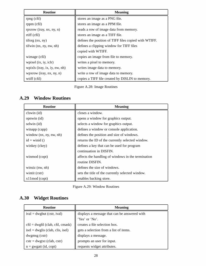
A.28 Image Routines

Routine Meaning

imgbox (nx, ny, nw, nh) defines a rectangle for PostScript/PDF output.

imgfin () terminates transfering of image data.

imgini () initializes transfering of image data.

imgmod (cmod) selects index or RGB mode.

imgsiz (nw, nh) defines an image size for PostScript/PDF output.

cbuf,n = rbfpng (nmax) stores an image as PNG file in a buffer. The memory

for the buffer is allocated by rbfpng.

rbmp (cfil) stores an image as a BMP file.

rimage (cfil) copies an image from memory to a file.

iclr = rpixel (ix, iy) reads a pixel from memory.

rpixls (iray, ix, iy, nw, nh) reads image data from memory.

27

Routine Meaning

rpng (cfil) stores an image as a PNG file.

rppm (cfil) stores an image as a PPM file.

rpxrow (iray, nx, ny, n) reads a row of image data from memory.

rtiff (cfil) stores an image as a TIFF file.

tiforg (nx, ny) defines the position of TIFF files copied with WTIFF.

tifwin (nx, ny, nw, nh) defines a clipping window for TIFF files

copied with WTIFF.

wimage (cfil) copies an image from file to memory.

wpixel (ix, iy, iclr) writes a pixel to memory.

wpixls (iray, ix, iy, nw, nh) writes image data to memory.

wpxrow (iray, nx, ny, n) write a row of image data to memory.

wtiff (cfil) copies a TIFF file created by DISLIN to memory.

Figure A.28: Image Routines

A.29 Window Routines

Routine Meaning

clswin (id) closes a window.

opnwin (id) opens a window for graphics output.

selwin (id) selects a window for graphics output.

winapp (capp) defines a window or console application.

window (nx, ny, nw, nh) defines the position and size of windows.

id = winid () returns the ID of the currently selected window.

winkey (ckey) defines a key that can be used for program

continuation in DISFIN.

winmod (copt) affects the handling of windows in the termination

routine DISFIN.

winsiz (nw, nh) defines the size of windows.

wintit (cstr) sets the title of the currently selected window.

x11mod (copt) enables backing store.

Figure A.29: Window Routines

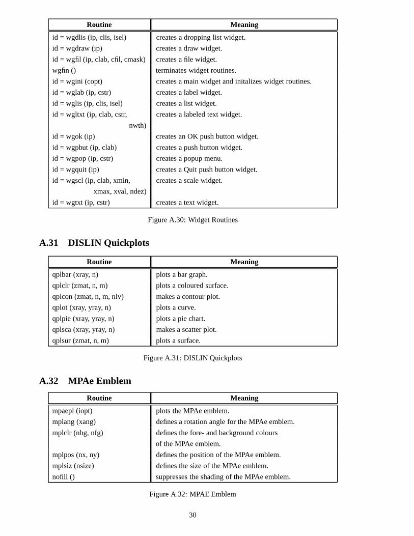
A.30 Widget Routines

Routine Meaning

ival = dwgbut (cstr, ival) displays a message that can be answered with

’Yes’ or ’No’.

cfil = dwgfil (clab, cfil, cmask) creates a file selection box.

isel = dwglis (clab, clis, isel) gets a selection from a list of items.

dwgmsg (cstr) displays a message.

cstr = dwgtxt (clab, cstr) prompts an user for input.

n = gwgatt (id, copt) requests widget attributes.

28

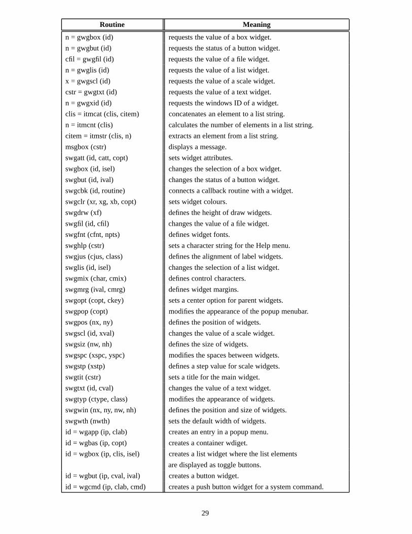
Routine Meaning

n = gwgbox (id) requests the value of a box widget.

n = gwgbut (id) requests the status of a button widget.

cfil = gwgfil (id) requests the value of a file widget.

n = gwglis (id) requests the value of a list widget.

x = gwgscl (id) requests the value of a scale widget.

cstr = gwgtxt (id) requests the value of a text widget.

n = gwgxid (id) requests the windows ID of a widget.

clis = itmcat (clis, citem) concatenates an element to a list string.

n = itmcnt (clis) calculates the number of elements in a list string.

citem = itmstr (clis, n) extracts an element from a list string.

msgbox (cstr) displays a message.

swgatt (id, catt, copt) sets widget attributes.

swgbox (id, isel) changes the selection of a box widget.

swgbut (id, ival) changes the status of a button widget.

swgcbk (id, routine) connects a callback routine with a widget.

swgclr (xr, xg, xb, copt) sets widget colours.

swgdrw (xf) defines the height of draw widgets.

swgfil (id, cfil) changes the value of a file widget.

swgfnt (cfnt, npts) defines widget fonts.

swghlp (cstr) sets a character string for the Help menu.

swgjus (cjus, class) defines the alignment of label widgets.

swglis (id, isel) changes the selection of a list widget.

swgmix (char, cmix) defines control characters.

swgmrg (ival, cmrg) defines widget margins.

swgopt (copt, ckey) sets a center option for parent widgets.

swgpop (copt) modifies the appearance of the popup menubar.

swgpos (nx, ny) defines the position of widgets.

swgscl (id, xval) changes the value of a scale widget.

swgsiz (nw, nh) defines the size of widgets.

swgspc (xspc, yspc) modifies the spaces between widgets.

swgstp (xstp) defines a step value for scale widgets.

swgtit (cstr) sets a title for the main widget.

swgtxt (id, cval) changes the value of a text widget.

swgtyp (ctype, class) modifies the appearance of widgets.

swgwin (nx, ny, nw, nh) defines the position and size of widgets.

swgwth (nwth) sets the default width of widgets.

id = wgapp (ip, clab) creates an entry in a popup menu.

id = wgbas (ip, copt) creates a container wdiget.

id = wgbox (ip, clis, isel) creates a list widget where the list elements

are displayed as toggle buttons.

id = wgbut (ip, cval, ival) creates a button widget.

id = wgcmd (ip, clab, cmd) creates a push button widget for a system command.

29

Routine Meaning

id = wgdlis (ip, clis, isel) creates a dropping list widget.

id = wgdraw (ip) creates a draw widget.

id = wgfil (ip, clab, cfil, cmask) creates a file widget.

wgfin () terminates widget routines.

id = wgini (copt) creates a main widget and initalizes widget routines.

id = wglab (ip, cstr) creates a label widget.

id = wglis (ip, clis, isel) creates a list widget.

id = wgltxt (ip, clab, cstr, creates a labeled text widget.

nwth)

id = wgok (ip) creates an OK push button widget.

id = wgpbut (ip, clab) creates a push button widget.

id = wgpop (ip, cstr) creates a popup menu.

id = wgquit (ip) creates a Quit push button widget.

id = wgscl (ip, clab, xmin, creates a scale widget.

xmax, xval, ndez)

id = wgtxt (ip, cstr) creates a text widget.

Figure A.30: Widget Routines

A.31 DISLIN Quickplots

Routine Meaning

qplbar (xray, n) plots a bar graph.

qplclr (zmat, n, m) plots a coloured surface.

qplcon (zmat, n, m, nlv) makes a contour plot.

qplot (xray, yray, n) plots a curve.

qplpie (xray, yray, n) plots a pie chart.

qplsca (xray, yray, n) makes a scatter plot.

qplsur (zmat, n, m) plots a surface.

Figure A.31: DISLIN Quickplots

A.32 MPAe Emblem

Routine Meaning

mpaepl (iopt) plots the MPAe emblem.

mplang (xang) defines a rotation angle for the MPAe emblem.

mplclr (nbg, nfg) defines the fore- and background colours

of the MPAe emblem.

mplpos (nx, ny) defines the position of the MPAe emblem.

mplsiz (nsize) defines the size of the MPAe emblem.

nofill () suppresses the shading of the MPAe emblem.

Figure A.32: MPAE Emblem

30

Appendix B

Examples

This appendix presents some examples of the DISLIN manual in Python coding. They can be found inthe DISLIN subdirectory python.

31

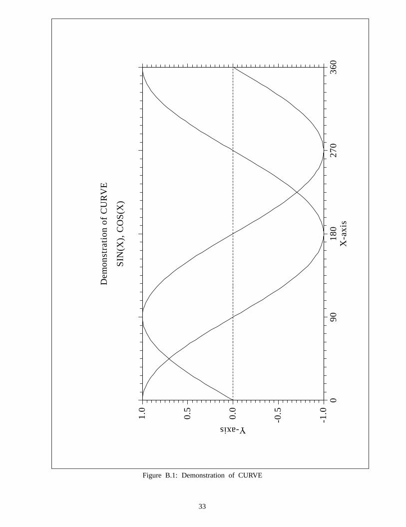
B.1 Demonstration of CURVE

#! /usr/bin/env pythonimport mathimport dislin

n = 101f = 3.1415926 / 180.x = range (n)y1 = range (n)y2 = range (n)for i in range (0,n):x[i] = i * 3.6v = i * 3.6 * fy1[i] = math.sin (v)y2[i] = math.cos (v)

dislin.metafl (’xwin’)dislin.disini ()dislin.complx ()dislin.pagera ()

dislin.axspos (450, 1800)dislin.axslen (2200, 1200)

dislin.name (’X-axis’, ’X’)dislin.name (’Y-axis’, ’Y’)

dislin.labdig (-1, ’X’)dislin.ticks (10, ’XY’)

dislin.titlin (’Demonstration of CURVE’, 1)dislin.titlin (’SIN (X), COS (X)’, 3)

dislin.graf (0., 360., 0., 90., -1., 1., -1., 0.5)dislin.title ()

dislin.color (’red’)dislin.curve (x, y1, n)dislin.color (’green’)dislin.curve (x, y2, n)

dislin.color (’foreground’)dislin.dash ()dislin.xaxgit ()dislin.disfin ()

32

09

01

80

27

03

60

X-a

xis

-1.0

-0.5

0.0

0.5

1.0

Y-axisD

em

on

stra

tio

n o

f C

UR

VE

SIN

(X),

CO

S(X

)

Figure B.1: Demonstration of CURVE

33

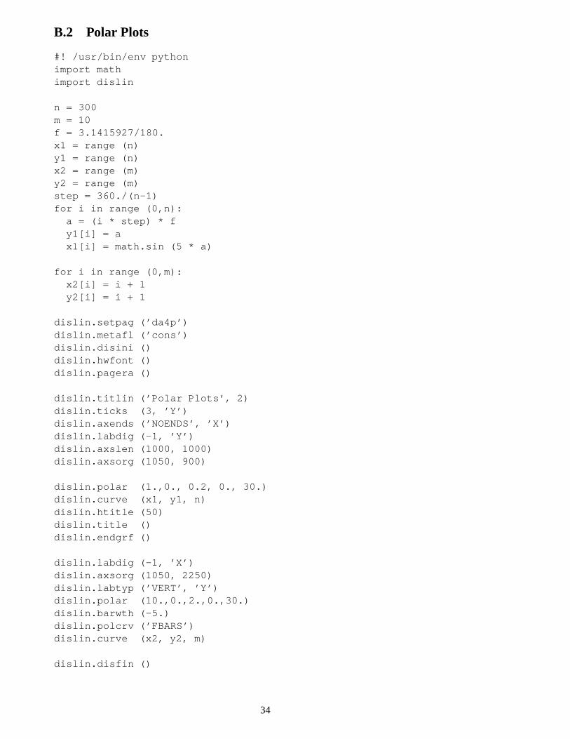
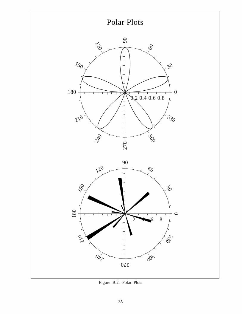
B.2 Polar Plots


n = 300m = 10f = 3.1415927/180.x1 = range (n)y1 = range (n)x2 = range (m)y2 = range (m)step = 360./(n-1)for i in range (0,n):a = (i * step) * fy1[i] = ax1[i] = math.sin (5 * a)

for i in range (0,m):x2[i] = i + 1y2[i] = i + 1

dislin.setpag (’da4p’)dislin.metafl (’cons’)dislin.disini ()dislin.hwfont ()dislin.pagera ()

dislin.titlin (’Polar Plots’, 2)dislin.ticks (3, ’Y’)dislin.axends (’NOENDS’, ’X’)dislin.labdig (-1, ’Y’)dislin.axslen (1000, 1000)dislin.axsorg (1050, 900)

dislin.polar (1.,0., 0.2, 0., 30.)dislin.curve (x1, y1, n)dislin.htitle (50)dislin.title ()dislin.endgrf ()

dislin.labdig (-1, ’X’)dislin.axsorg (1050, 2250)dislin.labtyp (’VERT’, ’Y’)dislin.polar (10.,0.,2.,0.,30.)dislin.barwth (-5.)dislin.polcrv (’FBARS’)dislin.curve (x2, y2, m)

dislin.disfin ()

34

0.2 0.4 0.6 0.80

30

60

90

120

150

180

210

240

27

0

300

330

Polar Plots

2 4 6 8

0

30

6090

120

150

18

0

210

240270

300

330

Figure B.2: Polar Plots

35

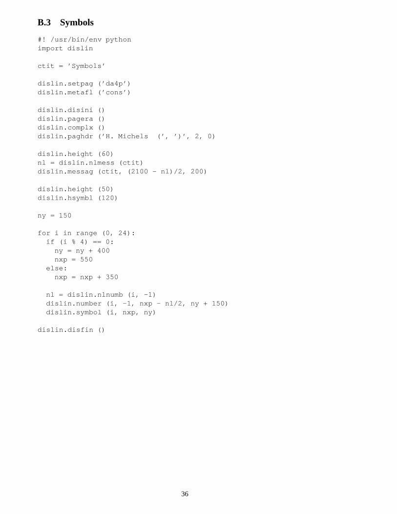
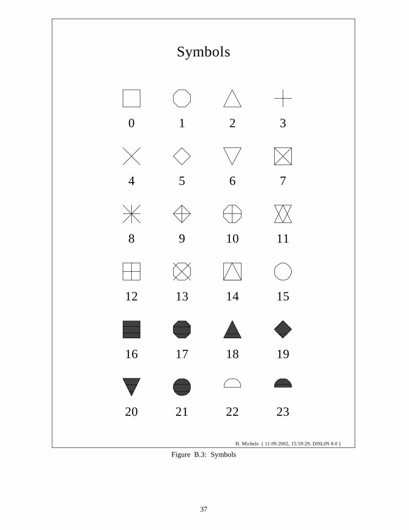
B.3 Symbols

#! /usr/bin/env pythonimport dislin

ctit = ’Symbols’

dislin.setpag (’da4p’)dislin.metafl (’cons’)

dislin.disini ()dislin.pagera ()dislin.complx ()dislin.paghdr (’H. Michels (’, ’)’, 2, 0)

dislin.height (60)nl = dislin.nlmess (ctit)dislin.messag (ctit, (2100 - nl)/2, 200)

dislin.height (50)dislin.hsymbl (120)

ny = 150

for i in range (0, 24):if (i % 4) == 0:ny = ny + 400nxp = 550

else:nxp = nxp + 350

nl = dislin.nlnumb (i, -1)dislin.number (i, -1, nxp - nl/2, ny + 150)dislin.symbol (i, nxp, ny)

dislin.disfin ()

36

H. Michels ( 11.09.2002, 15:59:29, DISLIN 8.0 )

Symbols

0 1 2 3

4 5 6 7

8 9 10 11

12 13 14 15

16 17 18 19

20 21 22 23

Figure B.3: Symbols

37

B.4 Logarithmic Scaling


ctit = ’Logarithmic Scaling’clab = [’LOG’, ’FLOAT’, ’ELOG’]


dislin.disini ()dislin.pagera ()dislin.complx ()dislin.axslen (1400, 500)

dislin.name (’X-axis’, ’X’)dislin.name (’Y-axis’, ’Y’)dislin.axsscl (’LOG’, ’XY’)

dislin.titlin (ctit, 2)

for i in range (0, 3):nya = 2650 - i * 800dislin.labdig (-1, ’XY’)if i == 1:dislin.labdig (1, ’Y’)dislin.name (’ ’, ’X’)

dislin.axspos (500, nya)dislin.messag (’Labels: ’ + clab[i], 600, nya - 400)dislin.labels (clab[i], ’XY’)dislin.graf (0., 3., 0., 1., -1., 2., -1., 1.)if i == 2:dislin.height (50)dislin.title ()

dislin.endgrf ()

dislin.disfin ()

38

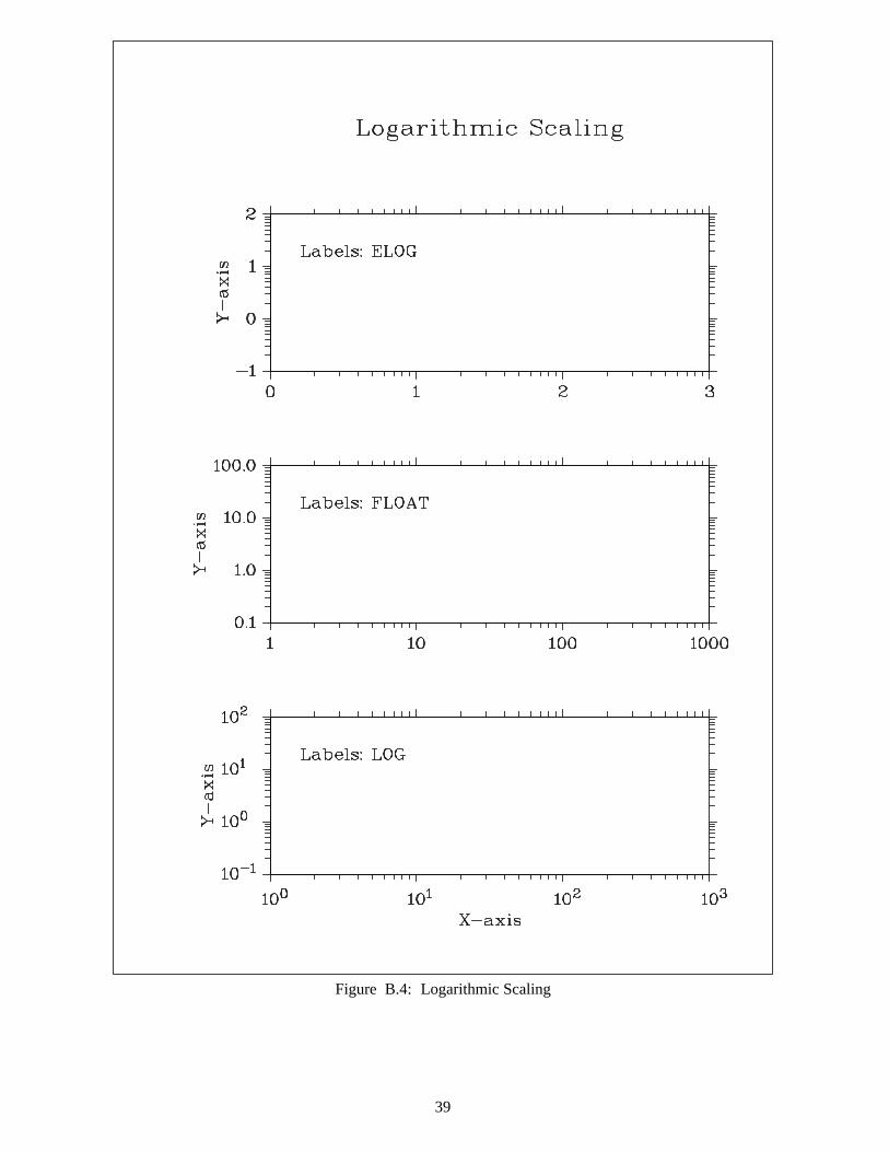
Figure B.4: Logarithmic Scaling

39

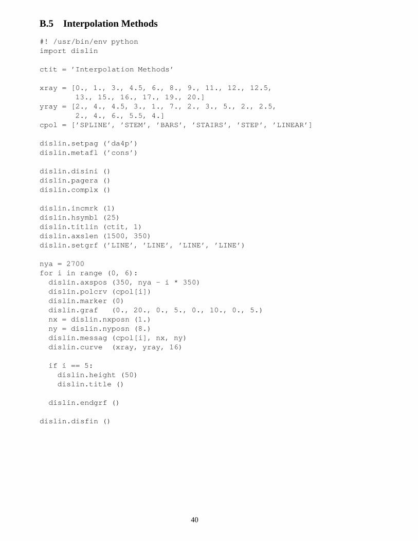
B.5 Interpolation Methods


ctit = ’Interpolation Methods’

xray = [0., 1., 3., 4.5, 6., 8., 9., 11., 12., 12.5,13., 15., 16., 17., 19., 20.]

yray = [2., 4., 4.5, 3., 1., 7., 2., 3., 5., 2., 2.5,2., 4., 6., 5.5, 4.]

cpol = [’SPLINE’, ’STEM’, ’BARS’, ’STAIRS’, ’STEP’, ’LINEAR’]


dislin.disini ()dislin.pagera ()dislin.complx ()

dislin.incmrk (1)dislin.hsymbl (25)dislin.titlin (ctit, 1)dislin.axslen (1500, 350)dislin.setgrf (’LINE’, ’LINE’, ’LINE’, ’LINE’)

nya = 2700for i in range (0, 6):dislin.axspos (350, nya - i * 350)dislin.polcrv (cpol[i])dislin.marker (0)dislin.graf (0., 20., 0., 5., 0., 10., 0., 5.)nx = dislin.nxposn (1.)ny = dislin.nyposn (8.)dislin.messag (cpol[i], nx, ny)dislin.curve (xray, yray, 16)

if i == 5:dislin.height (50)dislin.title ()

dislin.endgrf ()

dislin.disfin ()

40

Figure B.5: Interpolation Methods

41

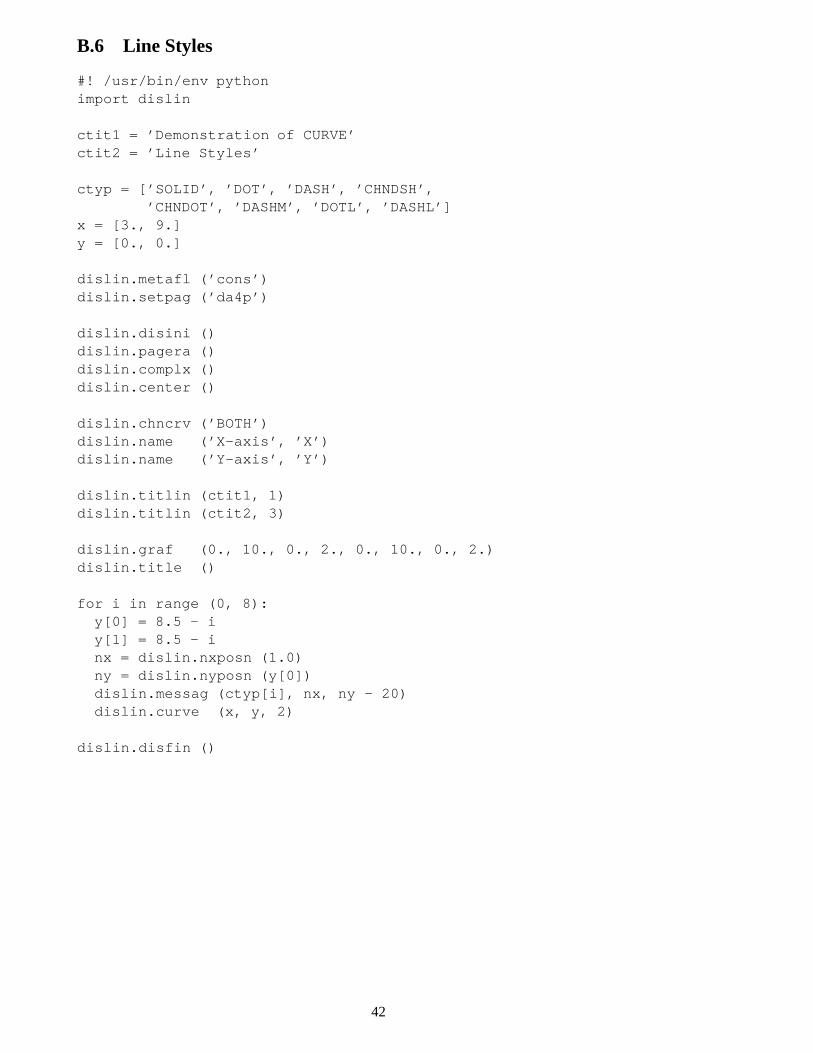
B.6 Line Styles


ctit1 = ’Demonstration of CURVE’ctit2 = ’Line Styles’

ctyp = [’SOLID’, ’DOT’, ’DASH’, ’CHNDSH’,’CHNDOT’, ’DASHM’, ’DOTL’, ’DASHL’]

x = [3., 9.]y = [0., 0.]

dislin.metafl (’cons’)dislin.setpag (’da4p’)

dislin.disini ()dislin.pagera ()dislin.complx ()dislin.center ()

dislin.chncrv (’BOTH’)dislin.name (’X-axis’, ’X’)dislin.name (’Y-axis’, ’Y’)

dislin.titlin (ctit1, 1)dislin.titlin (ctit2, 3)

dislin.graf (0., 10., 0., 2., 0., 10., 0., 2.)dislin.title ()

for i in range (0, 8):y[0] = 8.5 - iy[1] = 8.5 - inx = dislin.nxposn (1.0)ny = dislin.nyposn (y[0])dislin.messag (ctyp[i], nx, ny - 20)dislin.curve (x, y, 2)

dislin.disfin ()

42

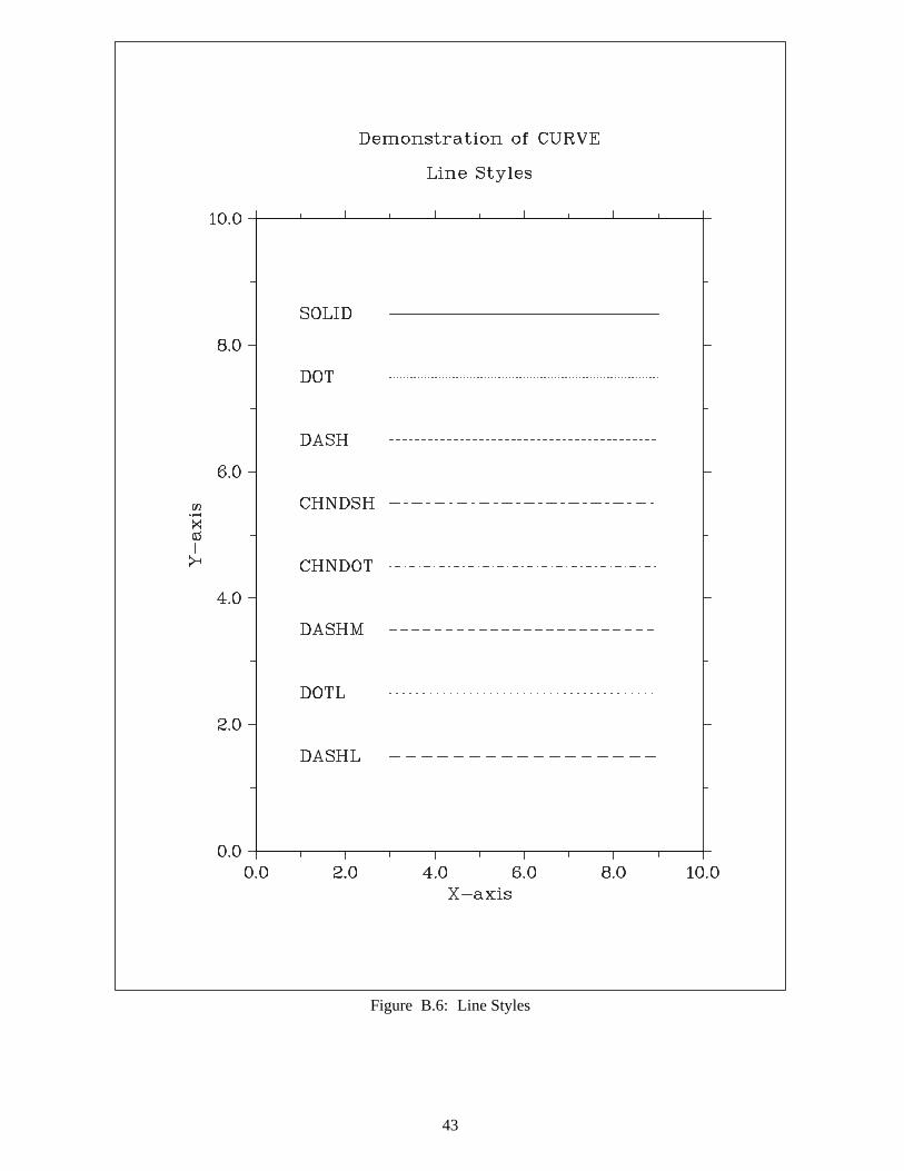
Figure B.6: Line Styles

43

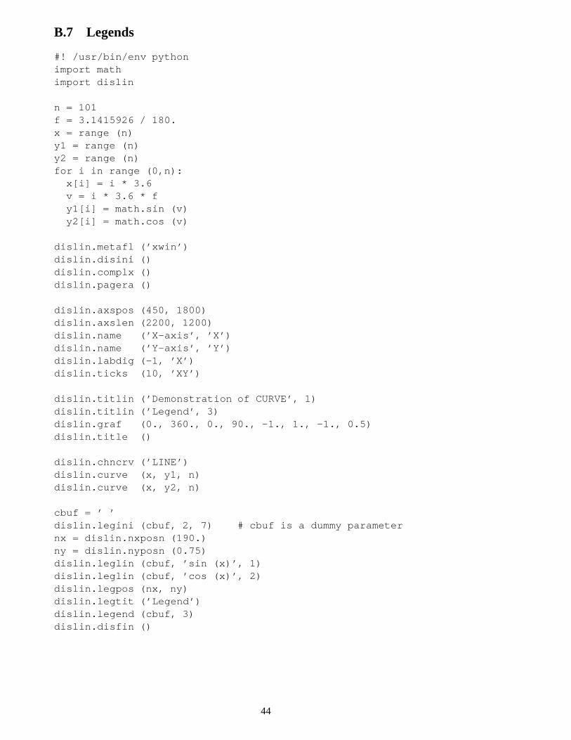
B.7 Legends


n = 101f = 3.1415926 / 180.x = range (n)y1 = range (n)y2 = range (n)for i in range (0,n):x[i] = i * 3.6v = i * 3.6 * fy1[i] = math.sin (v)y2[i] = math.cos (v)

dislin.metafl (’xwin’)dislin.disini ()dislin.complx ()dislin.pagera ()

dislin.axspos (450, 1800)dislin.axslen (2200, 1200)dislin.name (’X-axis’, ’X’)dislin.name (’Y-axis’, ’Y’)dislin.labdig (-1, ’X’)dislin.ticks (10, ’XY’)

dislin.titlin (’Demonstration of CURVE’, 1)dislin.titlin (’Legend’, 3)dislin.graf (0., 360., 0., 90., -1., 1., -1., 0.5)dislin.title ()

dislin.chncrv (’LINE’)dislin.curve (x, y1, n)dislin.curve (x, y2, n)

cbuf = ’ ’dislin.legini (cbuf, 2, 7) # cbuf is a dummy parameternx = dislin.nxposn (190.)ny = dislin.nyposn (0.75)dislin.leglin (cbuf, ’sin (x)’, 1)dislin.leglin (cbuf, ’cos (x)’, 2)dislin.legpos (nx, ny)dislin.legtit (’Legend’)dislin.legend (cbuf, 3)dislin.disfin ()

44

09

01

80

27

03

60

X-a

xis

-1.0

-0.5

0.0

0.5

1.0

Y-axis

De

mo

nst

rati

on

of

CU

RV

E

Le

ge

nd

Le

ge

nd

sin

(x)

cos

(x)

Figure B.7: Legends

45

B.8 Shading Patterns (AREAF)


ix = [0, 300, 300, 0]iy = [0, 0, 400, 400]ixp = [0, 0, 0, 0]iyp = [0, 0, 0, 0]

ctit = ’Shading Patterns (AREAF)’

dislin.metafl (’cons’)dislin.disini ()dislin.setvlt (’small’)dislin.pagera ()dislin.complx ()


nx0 = 335ny0 = 350

iclr = 0for i in range (0, 3):ny = ny0 + i * 600for j in range (0, 6):nx = nx0 + j * 400ii = i * 6 + jdislin.shdpat (ii)iclr = iclr + 1dislin.setclr (iclr)for k in range (0, 4):ixp[k] = ix[k] + nxiyp[k] = iy[k] + ny

dislin.areaf (ixp, iyp, 4)nl = dislin.nlnumb (ii, -1)nx = nx + (300 - nl) / 2dislin.color (’foreground’)dislin.number (ii, -1, nx, ny + 460)

dislin.disfin ()

46

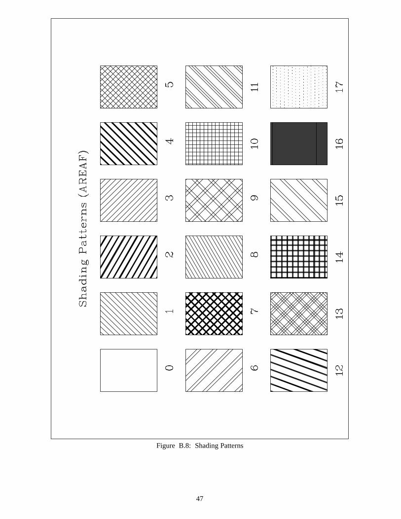
Figure B.8: Shading Patterns

47

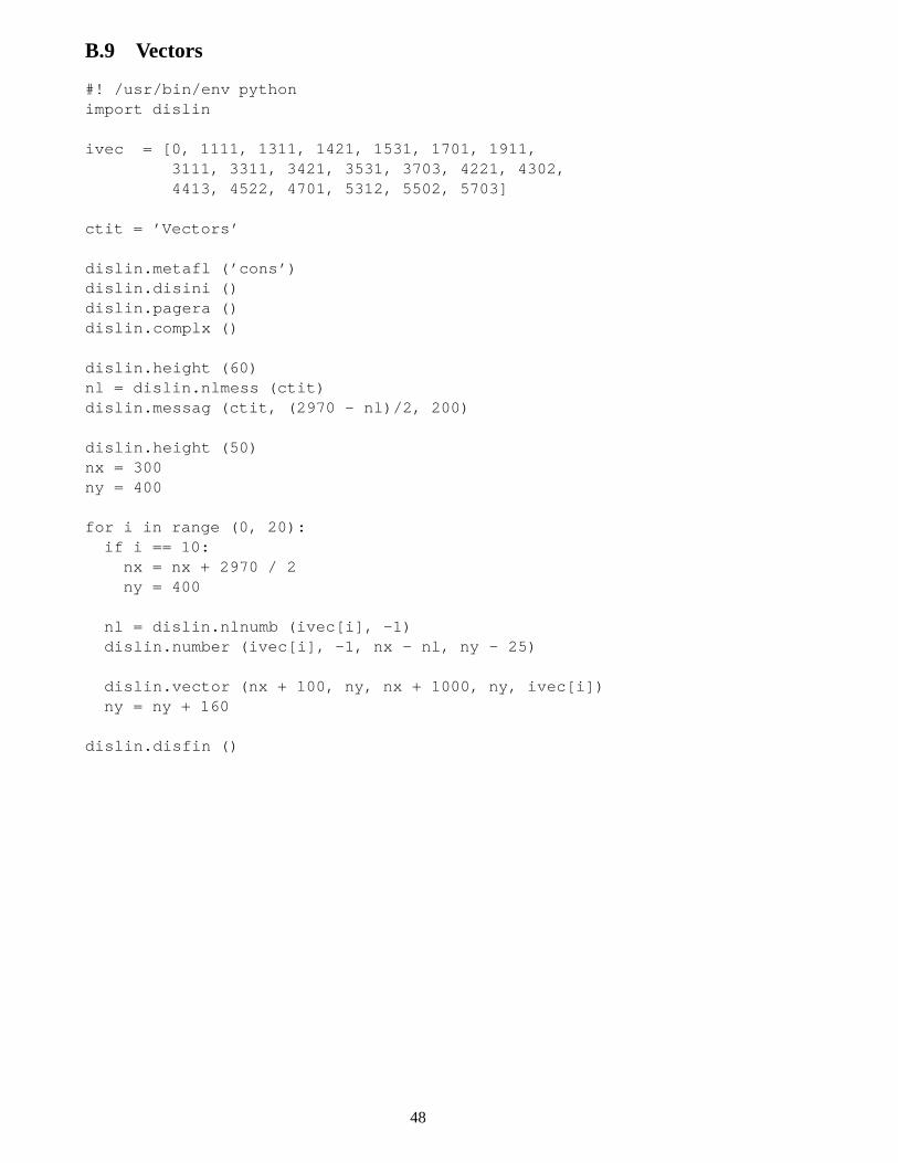
B.9 Vectors


ivec = [0, 1111, 1311, 1421, 1531, 1701, 1911,3111, 3311, 3421, 3531, 3703, 4221, 4302,4413, 4522, 4701, 5312, 5502, 5703]

ctit = ’Vectors’

dislin.metafl (’cons’)dislin.disini ()dislin.pagera ()dislin.complx ()


dislin.height (50)nx = 300ny = 400

for i in range (0, 20):if i == 10:nx = nx + 2970 / 2ny = 400

nl = dislin.nlnumb (ivec[i], -1)dislin.number (ivec[i], -1, nx - nl, ny - 25)

dislin.vector (nx + 100, ny, nx + 1000, ny, ivec[i])ny = ny + 160

dislin.disfin ()

48

Ve

cto

rs

0

11

11

13

11

14

21

15

31

17

01

19

11

31

11

33

11

34

21

35

31

37

03

42

21

43

02

44

13

45

22

47

01

53

12

55

02

57

03

Figure B.9: Vectors

49

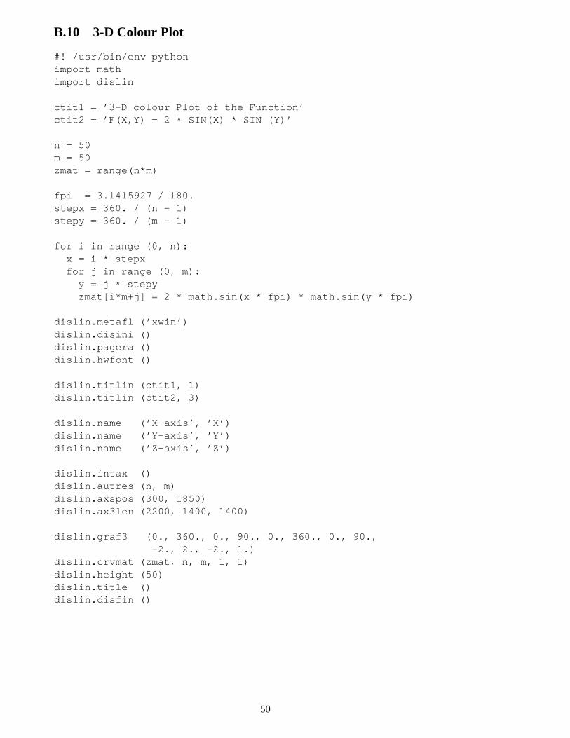
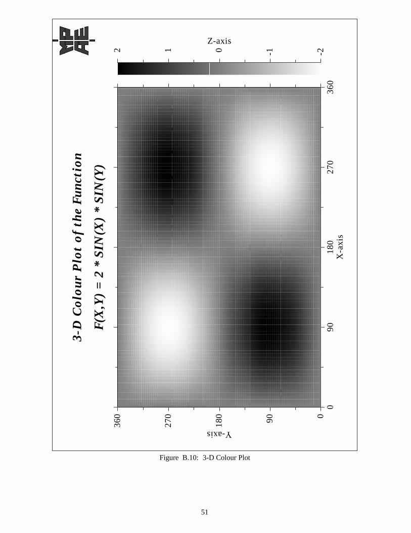
B.10 3-D Colour Plot


ctit1 = ’3-D colour Plot of the Function’ctit2 = ’F(X,Y) = 2 * SIN(X) * SIN (Y)’

n = 50m = 50zmat = range(n*m)

fpi = 3.1415927 / 180.stepx = 360. / (n - 1)stepy = 360. / (m - 1)

for i in range (0, n):x = i * stepxfor j in range (0, m):y = j * stepyzmat[i*m+j] = 2 * math.sin(x * fpi) * math.sin(y * fpi)

dislin.metafl (’xwin’)dislin.disini ()dislin.pagera ()dislin.hwfont ()


dislin.name (’X-axis’, ’X’)dislin.name (’Y-axis’, ’Y’)dislin.name (’Z-axis’, ’Z’)

dislin.intax ()dislin.autres (n, m)dislin.axspos (300, 1850)dislin.ax3len (2200, 1400, 1400)

dislin.graf3 (0., 360., 0., 90., 0., 360., 0., 90.,-2., 2., -2., 1.)

dislin.crvmat (zmat, n, m, 1, 1)dislin.height (50)dislin.title ()dislin.disfin ()

50

09

01

80

27

03

60

X-a

xis

090

18

0

27

0

36

0

Y-axis

-2-1012

Z-axis

3-D

Col

our

Plo

t of

the

Fun

ctio

n

F(X

,Y)

= 2

* S

IN(X

) *

SIN

(Y)

Figure B.10: 3-D Colour Plot

51

B.11 Surface Plot


ctit1 = ’Surface Plot (SURMAT)’ctit2 = ’F(X,Y) = 2 * SIN(X) * SIN (Y)’

n = 50m = 50zmat = range(n*m)


for i in range (0, n):x = i * stepxfor j in range (0, m):y = j * stepyzmat[i*m+j] = 2 * math.sin(x * fpi) * math.sin(y * fpi)

dislin.metafl (’cons’)dislin.setpag (’da4p’)dislin.disini ()dislin.pagera ()dislin.complx ()



dislin.name (’X-axis’, ’X’)dislin.name (’Y-axis’, ’Y’)dislin.name (’Z-axis’, ’Z’)

dislin.view3d (-5., -5., 4., ’ABS’)dislin.graf3d (0., 360., 0., 90., 0., 360., 0., 90.,

-3., 3., -3., 1.)dislin.height (50)dislin.title ()

dislin.color (’green’)dislin.surmat (zmat, n, m, 1, 1)dislin.disfin ()

52

Figure B.11: Surface Plot

53

B.12 Surface Plot


def myfunc (x, y, iopt):if iopt == 1:

xv = math.cos(x)*(3+math.cos(y))elif iopt == 2:

xv = math.sin(x)*(3+math.cos(y))else:

xv = math.sin(y)return xv

ctit1 = ’Surface Plot of the Parametric Function’ctit2 = ’[COS(t)*(3+COS(u)), SIN(t)*(3+COS(u)), SIN(u)]’

dislin.scrmod (’revers’)dislin.metafl (’cons’)dislin.setpag (’da4p’)dislin.disini ()dislin.pagera ()dislin.complx ()



dislin.name (’X-axis’, ’X’)dislin.name (’Y-axis’, ’Y’)dislin.name (’Z-axis’, ’Z’)dislin.intax ()

dislin.vkytit (-300)dislin.zscale (-1.,1.)dislin.surmsh (’on’)

dislin.graf3d (-4.,4.,-4.,1.,-4.,4.,-4.,1.,-3., 3., -3., 1)dislin.height (40)dislin.title ()

pi = 3.1415927step = 2 * pi / 30.dislin.surfcp (myfunc, 0., 2*pi, step, 0., 2*pi, step)dislin.disfin ()

54

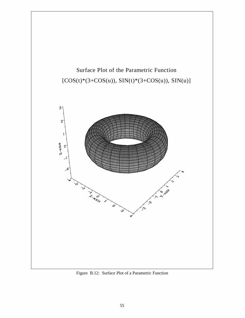
Surface Plot of the Parametric Function

[COS(t)*(3+COS(u)), SIN(t)*(3+COS(u)), SIN(u)]

Figure B.12: Surface Plot of a Parametric Function

55

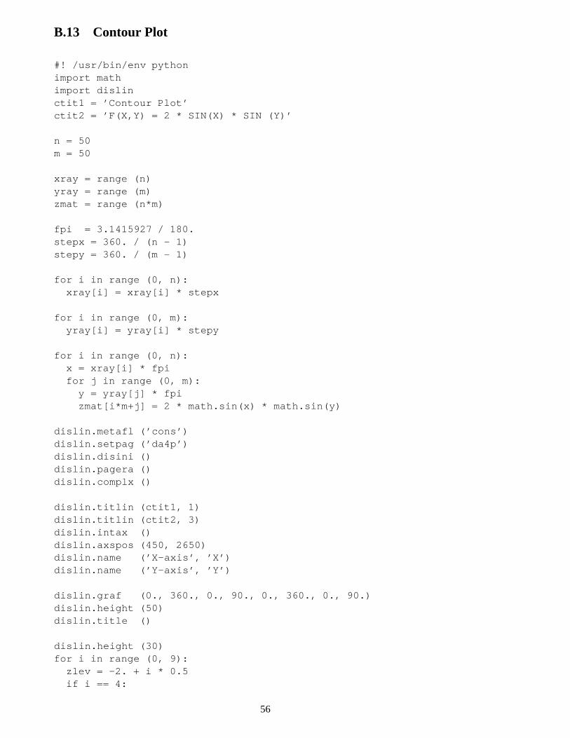
B.13 Contour Plot

#! /usr/bin/env pythonimport mathimport dislinctit1 = ’Contour Plot’ctit2 = ’F(X,Y) = 2 * SIN(X) * SIN (Y)’

n = 50m = 50

xray = range (n)yray = range (m)zmat = range (n*m)


for i in range (0, n):xray[i] = xray[i] * stepx

for i in range (0, m):yray[i] = yray[i] * stepy

for i in range (0, n):x = xray[i] * fpifor j in range (0, m):y = yray[j] * fpizmat[i*m+j] = 2 * math.sin(x) * math.sin(y)

dislin.metafl (’cons’)dislin.setpag (’da4p’)dislin.disini ()dislin.pagera ()dislin.complx ()

dislin.titlin (ctit1, 1)dislin.titlin (ctit2, 3)dislin.intax ()dislin.axspos (450, 2650)dislin.name (’X-axis’, ’X’)dislin.name (’Y-axis’, ’Y’)

dislin.graf (0., 360., 0., 90., 0., 360., 0., 90.)dislin.height (50)dislin.title ()

dislin.height (30)for i in range (0, 9):zlev = -2. + i * 0.5if i == 4:

56

dislin.labels (’NONE’, ’CONTUR’)else:dislin.labels (’FLOAT’, ’CONTUR’)

dislin.setclr ((i+1) * 28)dislin.contur (xray, n, yray, m, zmat, zlev)

dislin.disfin ()

57

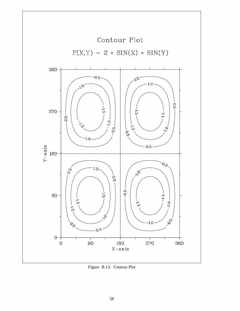
Figure B.13: Contour Plot

58

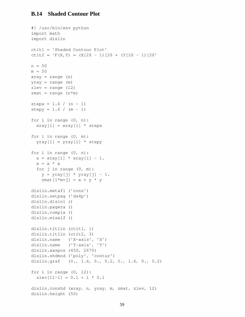
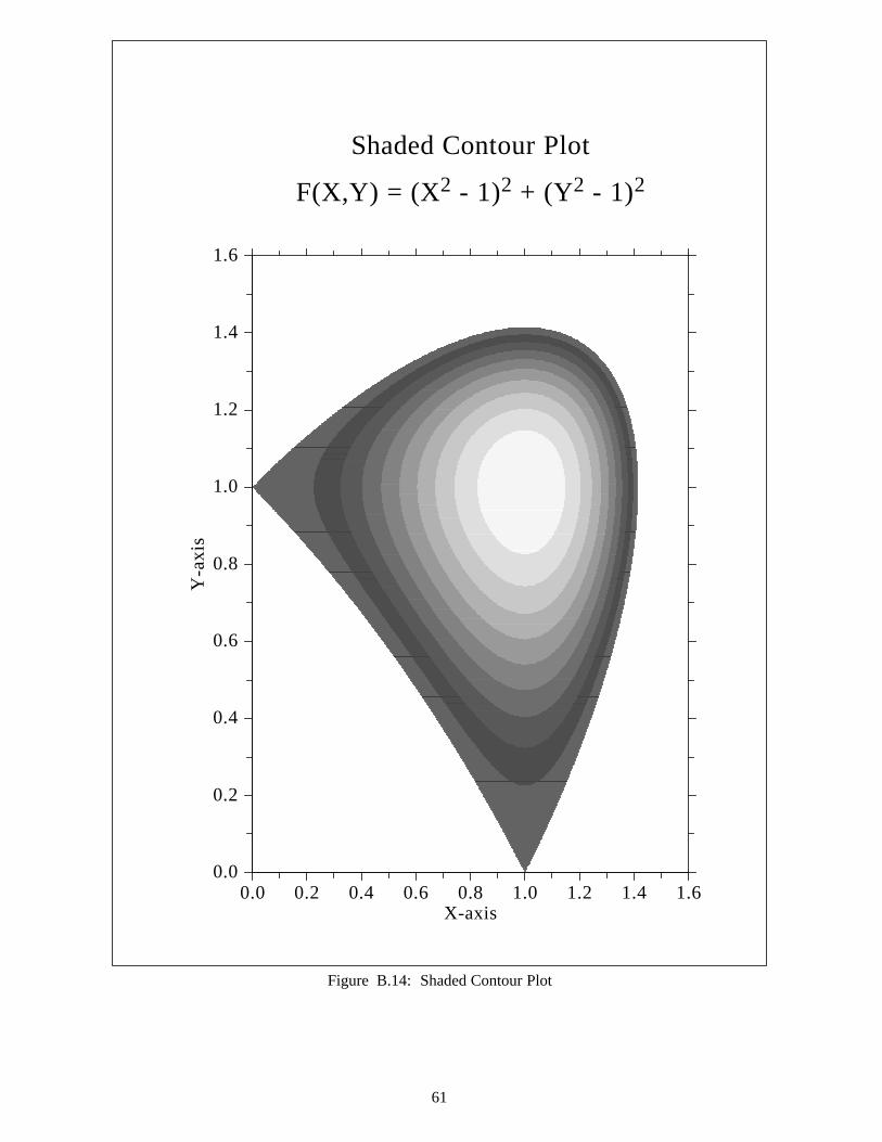
B.14 Shaded Contour Plot


ctit1 = ’Shaded Contour Plot’ctit2 = ’F(X,Y) = (X[2$ - 1)[2$ + (Y[2$ - 1)[2$’

n = 50m = 50xray = range (n)yray = range (m)zlev = range (12)zmat = range (n*m)

stepx = 1.6 / (n - 1)stepy = 1.6 / (m - 1)

for i in range (0, n):xray[i] = xray[i] * stepx

for i in range (0, m):yray[i] = yray[i] * stepy

for i in range (0, n):x = xray[i] * xray[i] - 1.x = x * xfor j in range (0, m):y = yray[j] * yray[j] - 1.zmat[i*m+j] = x + y * y

dislin.metafl (’cons’)dislin.setpag (’da4p’)dislin.disini ()dislin.pagera ()dislin.complx ()dislin.mixalf ()

dislin.titlin (ctit1, 1)dislin.titlin (ctit2, 3)dislin.name (’X-axis’, ’X’)dislin.name (’Y-axis’, ’Y’)dislin.axspos (450, 2670)dislin.shdmod (’poly’, ’contur’)dislin.graf (0., 1.6, 0., 0.2, 0., 1.6, 0., 0.2)

for i in range (0, 12):zlev[11-i] = 0.1 + i * 0.1

dislin.conshd (xray, n, yray, m, zmat, zlev, 12)dislin.height (50)

59

dislin.title ()dislin.disfin ()

60

0.0 0.2 0.4 0.6 0.8 1.0 1.2 1.4 1.6X-axis

0.0

0.2

0.4

0.6

0.8

1.0

1.2

1.4

1.6

Y-a

xis

Shaded Contour Plot

F(X,Y) = (X2 - 1)2 + (Y2 - 1)2

Figure B.14: Shaded Contour Plot

61

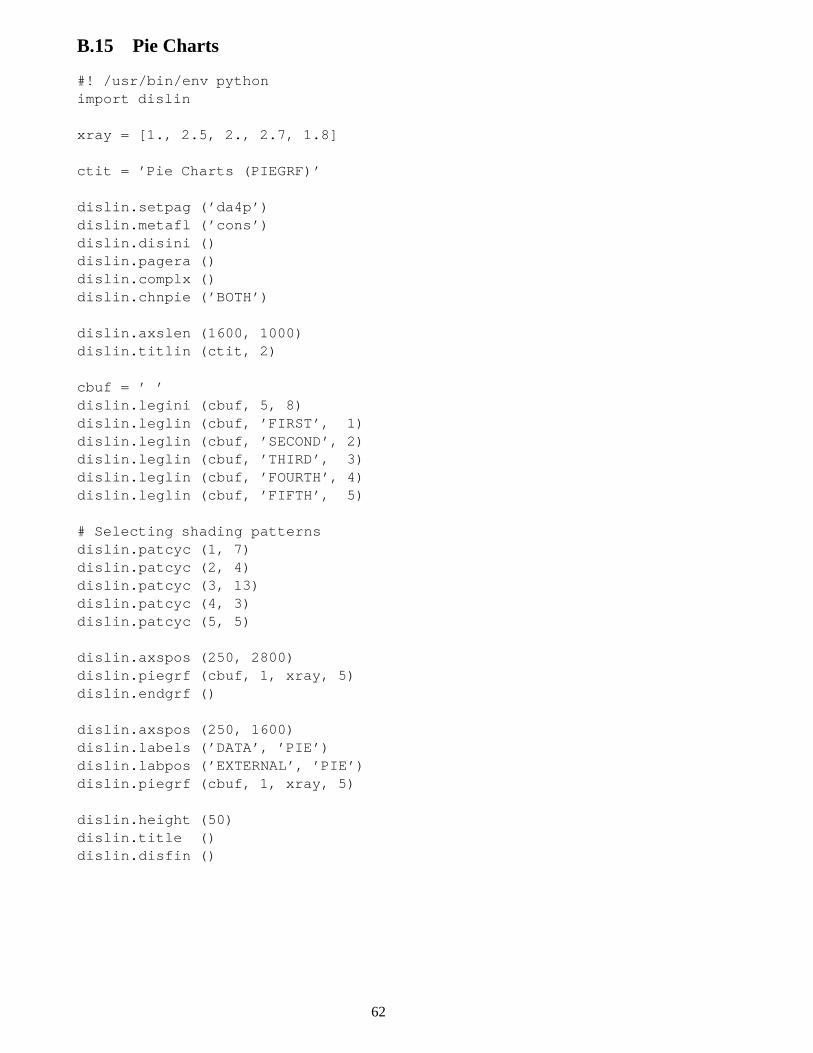
B.15 Pie Charts


xray = [1., 2.5, 2., 2.7, 1.8]

ctit = ’Pie Charts (PIEGRF)’

dislin.setpag (’da4p’)dislin.metafl (’cons’)dislin.disini ()dislin.pagera ()dislin.complx ()dislin.chnpie (’BOTH’)

dislin.axslen (1600, 1000)dislin.titlin (ctit, 2)

cbuf = ’ ’dislin.legini (cbuf, 5, 8)dislin.leglin (cbuf, ’FIRST’, 1)dislin.leglin (cbuf, ’SECOND’, 2)dislin.leglin (cbuf, ’THIRD’, 3)dislin.leglin (cbuf, ’FOURTH’, 4)dislin.leglin (cbuf, ’FIFTH’, 5)

# Selecting shading patternsdislin.patcyc (1, 7)dislin.patcyc (2, 4)dislin.patcyc (3, 13)dislin.patcyc (4, 3)dislin.patcyc (5, 5)

dislin.axspos (250, 2800)dislin.piegrf (cbuf, 1, xray, 5)dislin.endgrf ()

dislin.axspos (250, 1600)dislin.labels (’DATA’, ’PIE’)dislin.labpos (’EXTERNAL’, ’PIE’)dislin.piegrf (cbuf, 1, xray, 5)

dislin.height (50)dislin.title ()dislin.disfin ()

62

Figure B.15: Pie Charts

63

B.16 World Coastlines and Lakes


dislin.metafl (’xwin’)dislin.disini ()dislin.pagera ()dislin.complx ()


dislin.name (’Longitude’, ’X’)dislin.name (’Latitude’, ’Y’)dislin.titlin (’World Coastlines and Lakes’, 3)

dislin.labels (’MAP’, ’XY’)dislin.grafmp (-180., 180., -180., 90., -90., 90., -90., 30.)

dislin.gridmp (1, 1)dislin.color (’green’)dislin.world ()

dislin.color (’foreground’)dislin.height (50)dislin.title ()dislin.disfin ()

64

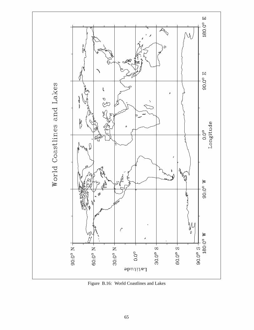
Figure B.16: World Coastlines and Lakes

65

66

Documents

DISLIN 8 - lab.demog.berkeley.edu · DISLIN 8.1 A Data Plotting Extension for the Programming Language Python by Helmut Michels