Disintermediation and Monetary Transmission in Canada

WP/06/84

Disintermediation and Monetary Transmission in Canada

Jorge Roldos

© 2006 International Monetary Fund WP/06/84

IMF Working Paper

Western Hemisphere Department

Disintermediation and Monetary Transmission in Canada

Prepared by Jorge Roldos1

Authorized for distribution by Tamim Bayoumi

March 2006

Abstract

This Working Paper should not be reported as representing the views of the IMF. The views expressed in this Working Paper are those of the author(s) and do not necessarily represent those of the IMF or IMF policy. Working Papers describe research in progress by the author(s) and are published to elicit comments and to further debate.

This paper studies changes in Canada’s monetary policy transmission, associated with the important changes in financial structure experienced in the 1990’s, using two methodologies. First, VAR models show a clear break in monetary transmission beginning in 1988, after changes in financial regulation initiated the process of financial disintermediation. Second, estimates of the interest rate elasticity of aggregate demand in IS equations increase in the 1990’s, suggesting that the systematic component of monetary policy has become more relevant. The ratio of direct to indirect finance, a measure of disintermediation, contributes to explain changes in the interest rate elasticity, suggesting an increased effectiveness of monetary policy associated with a larger use of market-based sources of finance. JEL Classification Numbers: E52, E3, C32 Keywords: Transmission of monetary policy; vector autoregression; new keynesian models. Author(s) E-Mail Address: [email protected]

1 I would like to thank Christopher Towe, Tamim Bayoumi, Ian Christensen, Francisco Covas and Calvin Schnure for helpful comments and suggestions. All remaining errors are my own.

Contents Page

I. Introduction....................................................................................................................3 II. Financial Deregulation and Disintermediation ..............................................................4 III. Changes in Monetary Transmission: Evidence from VAR Models ..............................5 IV. Changes in Monetary Transmission: Evidence from Structural Models .......................9 V. Conclusions and Policy Implications...........................................................................12 References................................................................................................................................14

Tables

1. Tests for Break in VAR Model in 1988:1....................................................................17 2. Tests for Break in VAR Model in 1993:2....................................................................18 3. Tests for Break in VAR Model in 1991:1....................................................................19 4. Variance Decompositions of GDP to Monetary Shock ...............................................20 5. Changes in the Standard Deviations of Shocks ...........................................................21 6. Estimates of Closed Economy IS Equation (1971:1–200:2) .......................................22 7. Estimates of Closed Economy IS Equation (Sample break in 1988:1) .......................23 8. Estimates of Open Economy IS Equation (1971:1–200:2)..........................................24 9. Estimates of Open Economy IS Equation (Sample break in 1988:1)..........................25 Figures

1. Nonfinancial Corporate Financing Sources, 1971–2005 .............................................26 2. Credit Flows, 1971–2005.............................................................................................27 3. Ratio of Direct to Indirect Private Lending, 1971–2005 .............................................28 4. Outstanding Credit, 1971–-2005..................................................................................29 5. Impulse-Response Functions from Benchmark VAR..................................................30 6. Impulse-Response Functions from VAR including Business Loans...........................31 7. Impulse-Response Functions from VAR including Asset Prices ................................32 8. Impulse-Response Functions from VAR including Asset Prices and Business Loans.................................................................................................33

- 2 -

- 3 -

I. INTRODUCTION

The financial system links monetary policy and the real economy. Thus, events or trends that affect the financial system can also change the monetary transmission mechanism. Over the last two decades, Canada’s financial system (as well as those in other industrialized countries) has been transformed by several rounds of financial deregulation, innovation, and disintermediation. This transformation has likely affected the transmission of monetary policy. Monetary transmission occurs through the impact of interest rates on components of aggregate demand, and the so-called credit channels—including constraints in the availability of loanable funds to banks and corporates. Proponents of the credit channel argue that the traditional channel cannot explain the magnitude, timing and compositional effects of the monetary policy actions in the U.S. economy (see Bernanke and Gertler, 1995). Credit market frictions give rise to a “financial accelerator” mechanism that amplifies and makes more persistent the impact of a monetary policy action on the economy. These credit market frictions depend on several features of the financial system, in particular the degree of securitization of the financial system (broadly understood as the development of securities markets versus banks) and the size and the state of the banking system (Cecchetti, 1999). The credit channel is more an enhancement mechanism than a truly independent or parallel channel of monetary transmission (Bernanke and Gertler, 1995). Earlier literature on the credit channel focused on the bank lending channel, that argued that monetary policy operated through the lack of substitutes in both the liability and asset side of banks’ balance sheets. In particular, it was argued that a monetary tightening would result in a reduction in excess reserves and a contraction in the supply of loans, and that this would have a direct negative impact on output. The evidence on this mechanism is somewhat mixed (see, for instance, Kashyap and Stein, 1994), and it is likely that with financial deregulation and innovation the importance of the bank lending channel has diminished. More recent literature has focused on a broader balance sheet channel, that states that a monetary contraction weakens firms’ financial positions—either directly through reduced cash flows or indirectly through the decline of the value of assets and/or collateral. The deterioration in firms’ financial condition increases the external finance premium, and the associated increase in the cost of capital, operates through a “financial accelerator” mechanism that enhances the impact of monetary policy actions in the real economy (Bernanke, Gertler, and Gilchrist, 1999). Recent evidence on the macroeconomic significance of these financial frictions is provided in Levin, Natalucci, and Zakrajsek (2004). This paper studies changes in Canada’s monetary policy transmission, associated with the important changes in financial structure experienced in the 1990s, using two methodologies. First, a series of vector autoregression (VAR) models are used to characterize the dynamics of output and prices after a monetary shock. Standard VAR models used to study monetary transmission of the type surveyed in Christiano, Eichenbaum, and Evans (1999) are extended with the inclusion of financial variables emphasized in the credit channel literature, and are tested for the existence of structural breaks or parameter instability around the dates of major changes in financial sector regulation. Second, the paper studies the impact of financial variables on structural econometric models of aggregate demand increasingly used by central

- 4 -

banks to conduct monetary policy analysis. In particular, the paper studies the impact of the ratio of direct (or market) to indirect (or intermediated) finance, a summary measure of disintermediation, on the interest rate sensitivity of aggregate demand. The paper is organized as follows. The next section documents some key changes in Canada’s financial structure, followed by an analysis of changes in monetary transmission using VAR and structural models. A concluding section discusses some implications for monetary policy.

II. FINANCIAL DEREGULATION AND DISINTERMEDIATION

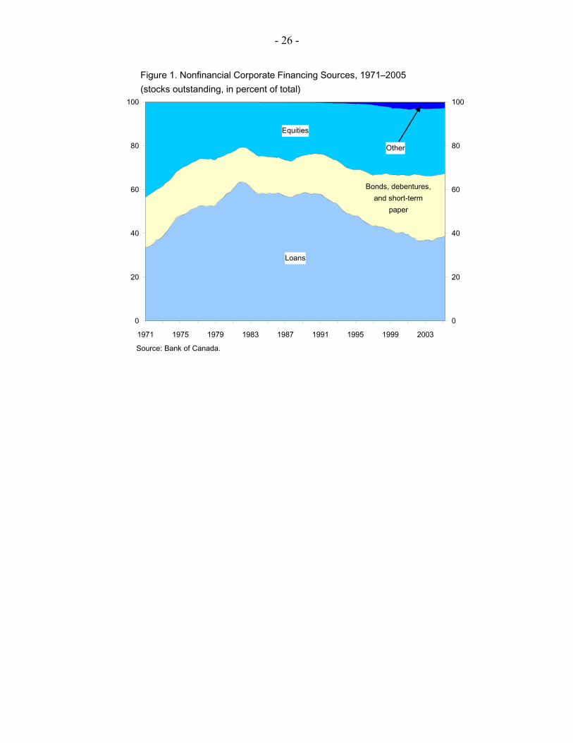
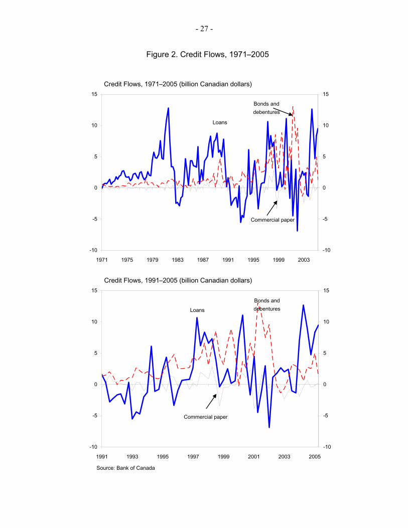
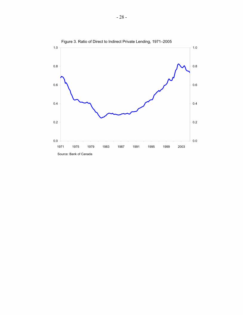
The Canadian financial system has experienced two important changes over the last two decades as a result of deregulation and financial innovation.2 First, the Canadian financial system has become more market-based, as corporates have increased the use of direct (or market) financing compared to indirect (or intermediated) financing. Second, there has been an increase in household’s access to credit, reflected in a rise in consumer and mortgage credit. The first trend is apparent in Figure 1, which shows a major decline in the share of bank lending in the composition of external financing of the nonfinancial business sector since the 1980s. During the 1970s, the rise in inflation and nominal interest rate uncertainty led the corporate sector to rely increasingly on short-term bank loans and much less on securities issuance. However, this trend was reversed in the 1980s, and bank lending as a source of funding for the corporate sector declined from approximately 60 percent in 1980 to under 40 percent in the 2000s. This was accompanied by an increase in the issuance of corporate bonds and commercial paper (Figure 2). This process of disintermediation is likely to have led to a reduction in the bank-dependency of borrowers and reduced constraints in the availability of loanable funds.3 These developments would be associated with a decline in the relative importance of the bank lending channel. However, they do not necessarily imply a reduction in the importance of the credit channel—as the cost of external finance, summarized in the “external finance premium,” may still operate as a key mechanism for the transmission of monetary policy. Changes in the regulatory framework, together with changes in global and Canadian financial market conditions, were major drivers of these structural changes. Calmes (2004) notes that significant Bank Act amendments in 1980, 1987, 1992, and 1997 contributed to (and were in part driven by) the sharp change in corporates’ funding mix. This is best summarized in Figure 3, that shows the increase in the ratio of direct-to-indirect lending beginning in the late

2 For a thorough account of these, as well as others, trends, see Freedman and Engert (2003) and Calmes (2004).

3 See Kashyap and Stein (1994) and Bernanke and Gertler (1995).

- 5 -

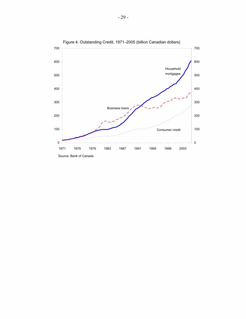
1980s. The increase follows a decade of stagnation in the 1980s, and a previous decline during the 1970s. The 1990s also saw an increase in equity issuance. This pattern of disintermediation, which parallels changes in other countries, has been accompanied by a switch in banks’ activities, from providing loans to large corporates to underwriting and other securities activities. In particular, Calmes (2004) notes that the 1987 amendments to the Bank Act allowed bank to conduct brokerage activates and that banks made substantial investments in the securities business between 1987 and 1989. Nonetheless, banks continue to be the main providers of loans to the medium-and-small enterprise sector. Also, several indicators show that the Canadian banking system has continued to grow despite their decreasing share of the lending business—especially when off-balance sheet activities are included (see Calmes, 2004). The second trend is the growth in credit to the household sector (broadly defined as persons and unincorporated businesses), which rose from just under 50 percent of GDP in the first half of the 1980s to almost 70 percent of GDP in 2001 (see Freedman and Engert, 2003). This steady increase has been driven by the growth of consumer and mortgage credit, associated to the decline in inflation and the evolution of housing prices (Figure 4). Indeed, consumer credit as a share of the total (business and consumer credit), increased from 42 percent in 1982 to 55 percent in 2005. This second trend, also shared by other industrialized nations, raises the importance of the household sector and has the potential of strengthening again the bank lending channel and/or the financial accelerator—that would work here more directly through housing prices and collateral. Although the securitization of mortgages has had a profound impact on monetary transmission in the United States (Estrella, 2002), mortgage securitization has advanced at a much slower pace in Canada (Freedman and Engert, 2003). The next sections of the paper explore how financial variables may have changed the monetary transmission mechanism. This is done first by looking at the impact of financial variables in traditional VAR models, and second by testing the impact of such variables in structural econometric models.

III. CHANGES IN MONETARY TRANSMISSION: EVIDENCE FROM VAR MODELS

Changes in monetary transmission associated with these changes in financial structure can be analyzed with VAR models, where a minimum structure is imposed and monetary shocks are identified as innovations to the interest rate equation. Standard VAR models used in studies of monetary transmission include a set of endogenous variables (output and prices), and a and an interest rate equation that captures a general monetary policy rule that affects the endogenous variables with a lag.4 Given the small open economy nature of Canada, the

4 This is the standard recursivity assumption, see Christiano, Eichenbaum, and Evans, 1999, and Favero, 2001.

- 6 -

exchange rate is included in the model after the interest rate equation, together with a set of exogenous variables X.5 The benchmark VAR model has the representation: 1( ) ( )t t t tY A L Y B L X u−= + + (1) where [ , , , ]t t t t tY y p R S= (2) and y is quarterly GDP, p is the GDP deflator, R is the 3 month T-bill rate,6 and S is the exchange rate. The vector of exogenous variables is given by [ , , ]US US

t t t tX y R cp= (3) where ,US

ty is U.S. GDP, USR is the Federal Funds rate, and cp is an index of world commodity prices. This benchmark VAR model is then extended with a block of financial variables F, suggested by the credit channel literature. These includes quantity variables, aimed at capturing the role/existence of alternative sources of funding for the corporate and household sectors, as well as asset price variables, aimed to capture the role of collateral and the “external finance premium.”7 The VAR models are estimated in levels using quarterly data from 1971, the beginning of the floating exchange rate period, to 2005. As in most VAR models of the monetary transmission mechanism, we do not perform an explicit analysis of the long run behavior of the economy.

5 The exogenous variables included are U.S. GDP and federal funds rate, and an index of world commodity prices.

6 Although the overnight rate is the Bank of Canada monetary policy instrument, and the best variable to summarize the monetary policy stance (Fung and Yuan, 2000), it is rather unstable in the first part of the sample. Thus, we use the T-bill rate that is highly correlated with the overnight rate, and is also the variable used in several EU studies that will serve as comparisons to the Canada case.

7 The variables included were: total loans to businesses and households; securities (bond, equities and commercial paper), and ratios that micro studies have found relevant for the credit channel (such as the ratio of commercial paper to business loans; see Kashyap and Stein, 1994). The price variables included spreads on loans, commercial paper and bonds, as well as stock and housing prices (and an aggregate asset price index, with equal weights of both of them).

- 7 -

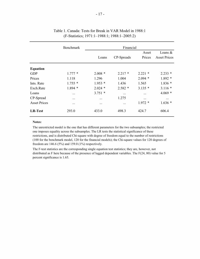
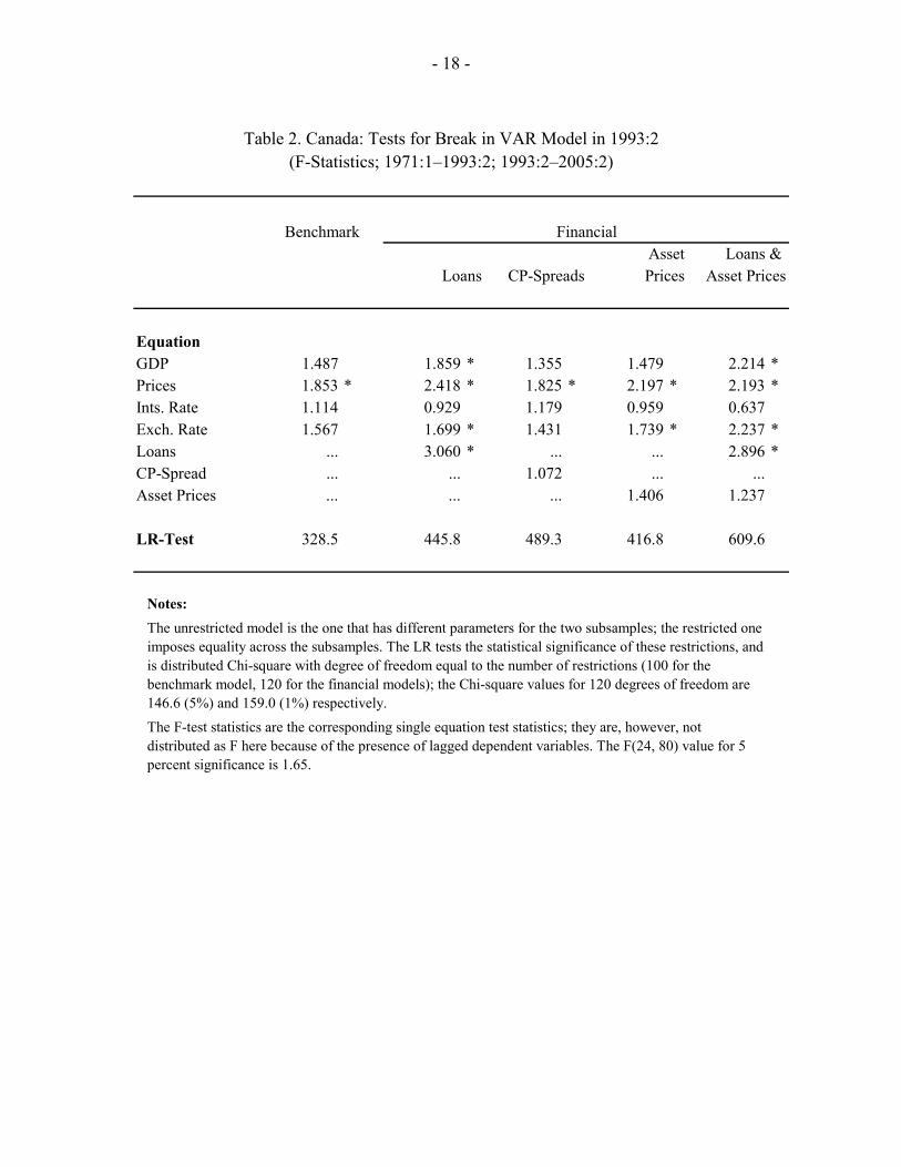
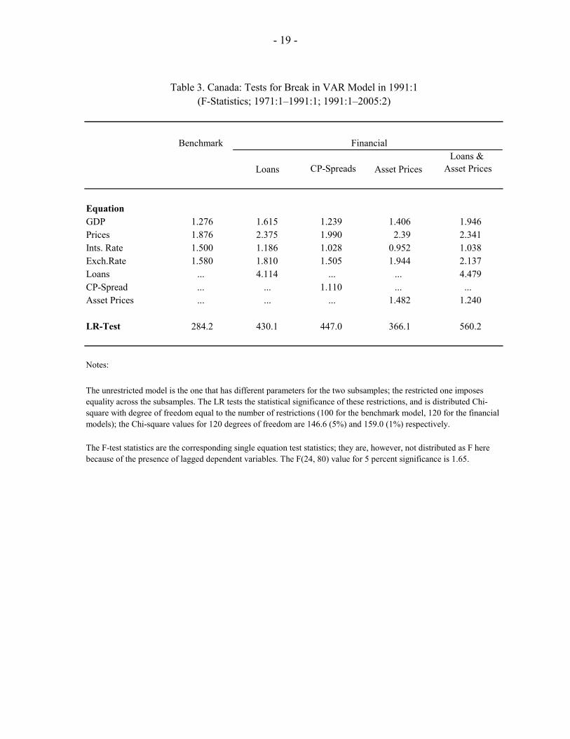
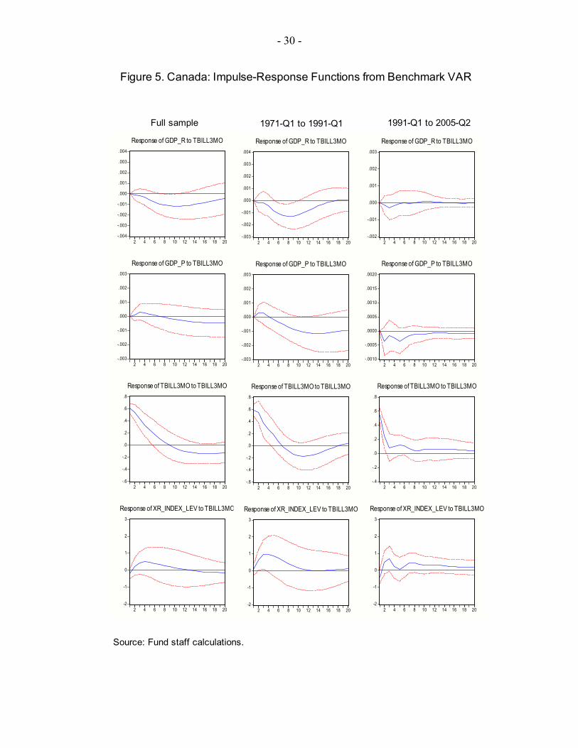
By doing the analysis in levels we allow for implicit cointegrating relationships in the data, but we do not explicitly impose cointegration. Imposing cointegrating restrictions on a VAR in levels could increase efficiency in the estimation, but this would be at the cost of potential inconsistencies if the incorrect identifying restrictions are imposed. Since the monetary transmission mechanism is a short-run phenomenon, most researchers prefer to employ unrestricted VARs in levels to evaluate impulse responses over the short to medium run (Favero, 2001). The dynamics of Canada’s output and prices are broadly similar to those found for the United States, the European Union, the United Kingdom, and Japan, using similar benchmark VAR models. 8 The impulse responses for the benchmark VAR for Canada for the full sample following a monetary shock are presented in the left-hand column of Figure 5. The decline in output after a contractionary monetary policy shock is somewhat smoother and more persistent in Canada, while the sluggish decline in prices (with an initial spike consistent with the so-called “price puzzle”) is similar to most other industrialized countries. The exchange rate appreciates for a period of about three years, but the results are not statistically significant for the full sample. Although the responses to a monetary shock during the full sample are consistent with other industrialized countries, the lack of significance and the knowledge of important regime changes9 suggest the possibility of a structural break in the statistical model in the late 1980s or early 1990s. Statistical tests for structural breaks at the dates when key changes to the Bank Act were implemented (1988:1 and 1993:2, as suggested by Calmes, 2004) confirm such breaks for both the benchmark and financial VARs (see the last line in Tables 1 and 2).10 The instability of the VAR coefficients is confirmed with likelihood-ratio tests for all VAR models at the 5 percent confidence levels. The second and third columns of Figure 5 show that the impulse responses in the first sub sample (1971:1–1991:1) are more tightly estimated and show a statistically significant decline in output between the 5th and 10th quarters. Prices fall more gradually and persistently, while the exchange rate appreciates sharply on impact and returns to its baseline level afterwards. However, the impulse responses for the second sub sample (1991:1–2005:2) show a very different shape and are statistically insignificant.11 8 See respectively, Christiano, Eichenbaum and Evans (1999), Peersman and Smets (2001), Bean, Larsen and Nikolov (2002) and Morsink and Bayoumi (2001).

9 In both financial regulation and in monetary policy; on the latter, see Atoyan, (2005).

10 The relatively small sample does not provide the degrees of freedom necessary to perform continuous break tests and let the data show the true break point. Tests for an intermediate date, 1991:1, reported in Table 3, yield results that are qualitatively similar to those of the second break test.

11 A similar pattern arises for the different components of aggregate demand: private consumption falls smoothly but persistently between the 4th and 10th quarters, investment

(continued…)

- 8 -

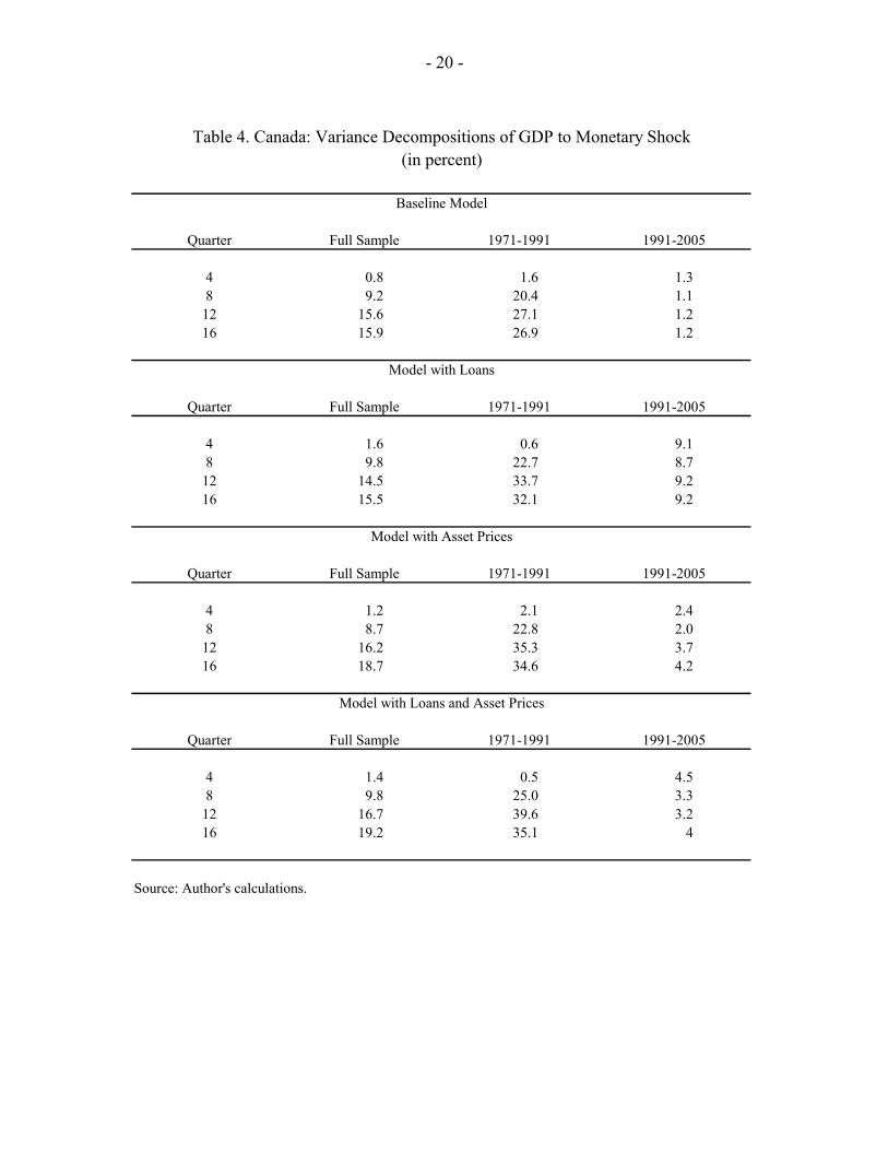
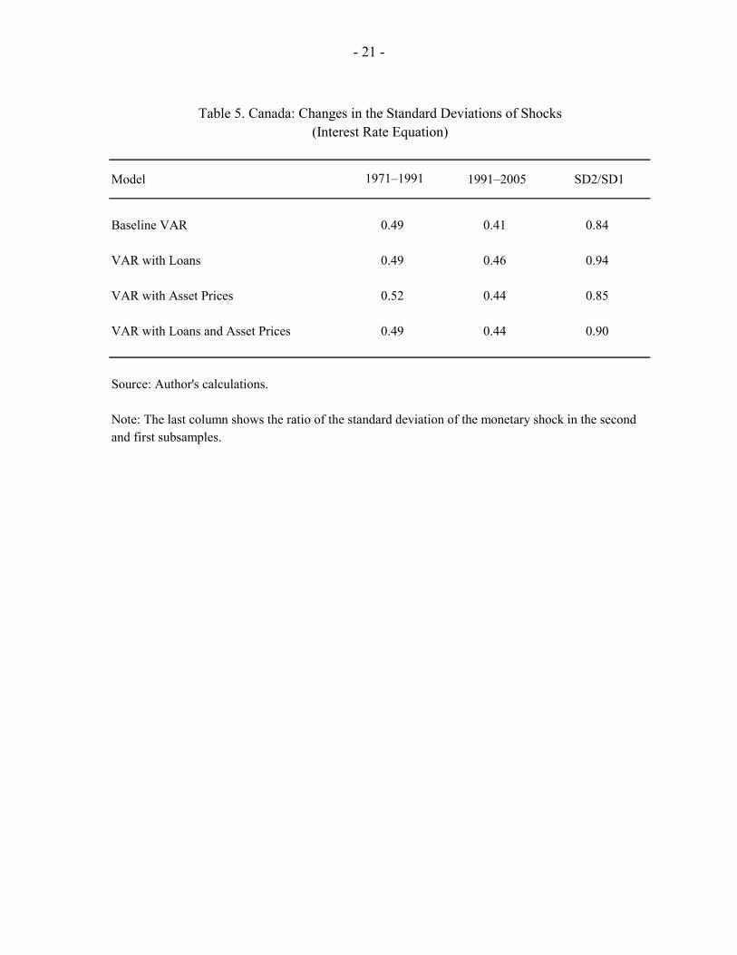
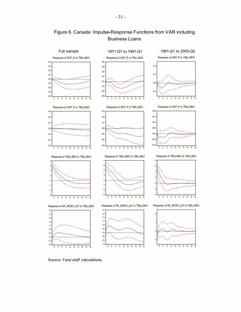
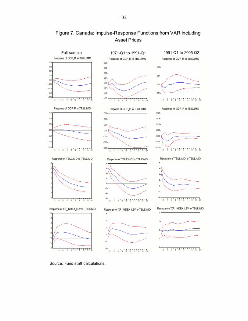
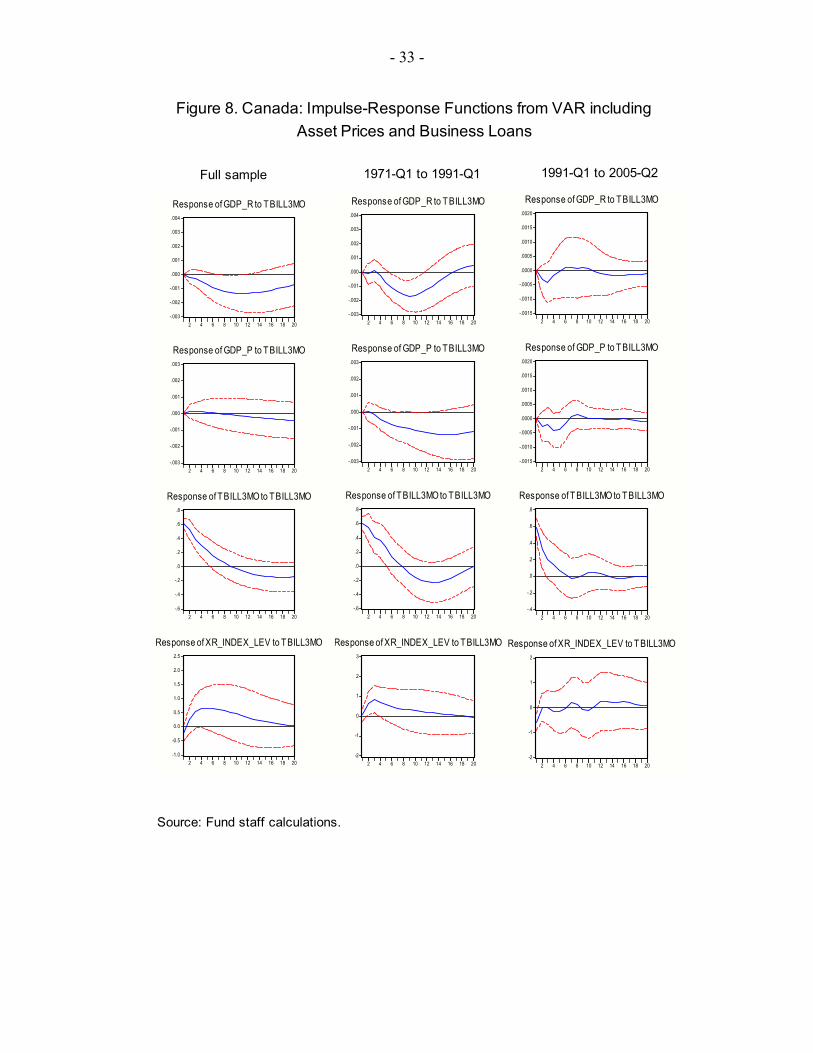
The extended VARs provide a tighter and improved characterization of the dynamics of macro variables after a monetary shock, especially for the first sub sample. The variables added included both asset prices and quantities, and the ones that contributed to an improved characterization of the transmission of interest shocks to output and prices were business loans (Figure 5), and asset prices (Figures 6 and 7). In particular, when each of these variables was added to the benchmark VAR, a statistically significant recession and a more tightly estimated response of the price level decline emerged for the first sub sample, and the appreciation of the exchange rate after the increase in interest rates becomes statistically significant. More important, the contribution of the interest rate shock to the variance of output fluctuations (as measured by the variance decompositions) increases markedly in the models with financial variables, suggesting that their addition contributes to a richer set of dynamic interactions and an improved characterization of the transmission mechanism. Table 4 shows that in the first sub-sample, monetary shocks explain close to 35-40 percent of the variance of output in the financial models, while they explain around 27 percent in the baseline model. The dynamics of output following a monetary shock seem to have changed earlier in the sample period that the dynamics of prices. The F-tests for individual equations in each VAR show a structural break for the output equations in all the models by 1988, while the price equation changes are more robust in the early 1990s (Tables 1-3). This is consistent with changes in output been associated with the earlier changes in financial structure, and those in prices been more closely associated with the changes in the monetary regime in the early 1990s. The fact that the responses to a monetary shock have become weaker in the more recent sub sample can be interpreted as reflecting the fact that the systematic component of monetary policy (i.e., the one captured by the monetary policy rule) has become more important with the increased transparency and other institutional improvements associated with the adoption of inflation targeting. This is consistent with a decline in the importance of monetary shocks, i.e. the unexpected part of monetary policy captured by the VAR shocks. Indeed, Table 5 shows that the standard deviation of the monetary shocks in the second sub sample is systematically smaller than in the first sub sample. Similar conclusions, both in terms of the instability of monetary VAR models, and the increasing role of systematic monetary policy, have been found for the United States.12

falls three times as much as consumption, and residential investment falls more than total investment. In the second sub sample, residential investment falls significantly during the first year only (despite the mild response in GDP), and several of the results are statistically insignificant.

12 See Bernanke, Gertler, and Watson, 1997, and Boivin and Giannoni, 2002.

- 9 -

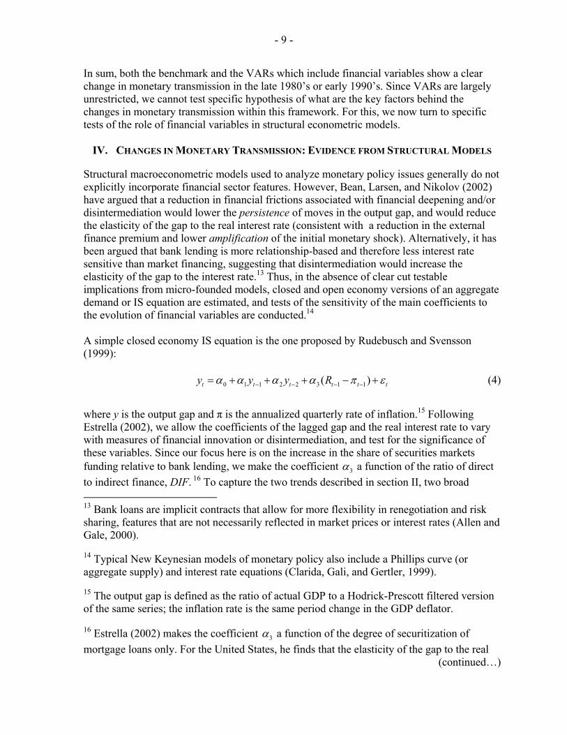
In sum, both the benchmark and the VARs which include financial variables show a clear change in monetary transmission in the late 1980’s or early 1990’s. Since VARs are largely unrestricted, we cannot test specific hypothesis of what are the key factors behind the changes in monetary transmission within this framework. For this, we now turn to specific tests of the role of financial variables in structural econometric models.

IV. CHANGES IN MONETARY TRANSMISSION: EVIDENCE FROM STRUCTURAL MODELS

Structural macroeconometric models used to analyze monetary policy issues generally do not explicitly incorporate financial sector features. However, Bean, Larsen, and Nikolov (2002) have argued that a reduction in financial frictions associated with financial deepening and/or disintermediation would lower the persistence of moves in the output gap, and would reduce the elasticity of the gap to the real interest rate (consistent with a reduction in the external finance premium and lower amplification of the initial monetary shock). Alternatively, it has been argued that bank lending is more relationship-based and therefore less interest rate sensitive than market financing, suggesting that disintermediation would increase the elasticity of the gap to the interest rate.13 Thus, in the absence of clear cut testable implications from micro-founded models, closed and open economy versions of an aggregate demand or IS equation are estimated, and tests of the sensitivity of the main coefficients to the evolution of financial variables are conducted.14 A simple closed economy IS equation is the one proposed by Rudebusch and Svensson (1999): 0 1 1 2 2 3 1 1( )t t t t t ty y y Rα α α α π ε− − − −= + + + − + (4)

where y is the output gap and π is the annualized quarterly rate of inflation.15 Following Estrella (2002), we allow the coefficients of the lagged gap and the real interest rate to vary with measures of financial innovation or disintermediation, and test for the significance of these variables. Since our focus here is on the increase in the share of securities markets funding relative to bank lending, we make the coefficient 3α a function of the ratio of direct to indirect finance, DIF. 16 To capture the two trends described in section II, two broad 13 Bank loans are implicit contracts that allow for more flexibility in renegotiation and risk sharing, features that are not necessarily reflected in market prices or interest rates (Allen and Gale, 2000).

14 Typical New Keynesian models of monetary policy also include a Phillips curve (or aggregate supply) and interest rate equations (Clarida, Gali, and Gertler, 1999).

15 The output gap is defined as the ratio of actual GDP to a Hodrick-Prescott filtered version of the same series; the inflation rate is the same period change in the GDP deflator.

16 Estrella (2002) makes the coefficient 3α a function of the degree of securitization of mortgage loans only. For the United States, he finds that the elasticity of the gap to the real

(continued…)

- 10 -

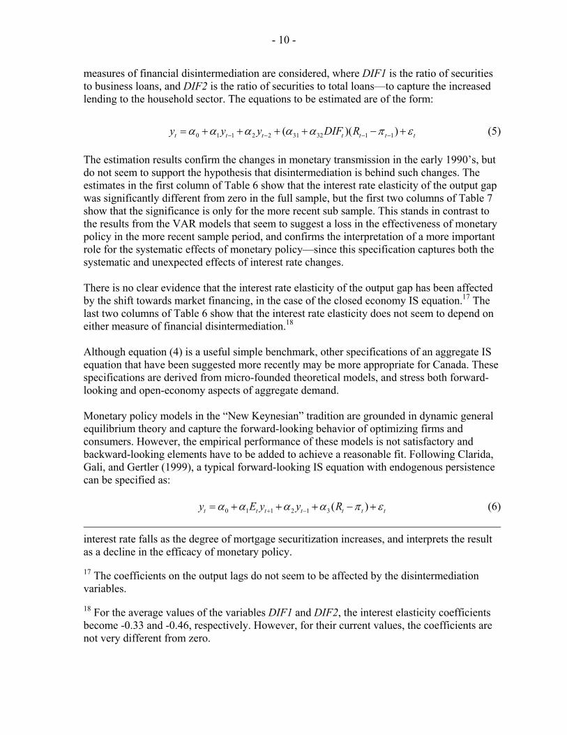
measures of financial disintermediation are considered, where DIF1 is the ratio of securities to business loans, and DIF2 is the ratio of securities to total loans—to capture the increased lending to the household sector. The equations to be estimated are of the form:

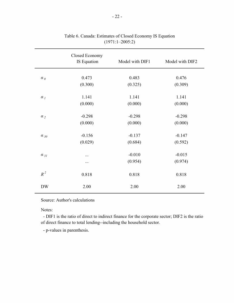
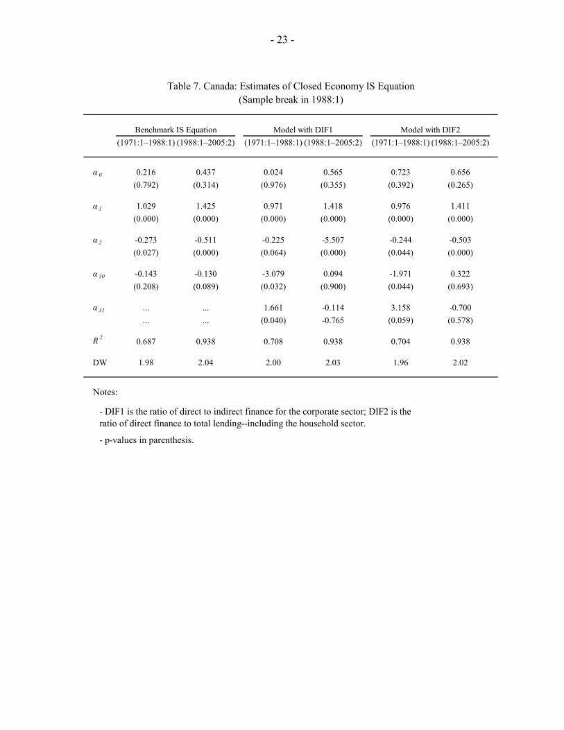
0 1 1 2 2 31 32 1 1( )( )t t t t t t ty y y DIF Rα α α α α π ε− − − −= + + + + − + (5) The estimation results confirm the changes in monetary transmission in the early 1990’s, but do not seem to support the hypothesis that disintermediation is behind such changes. The estimates in the first column of Table 6 show that the interest rate elasticity of the output gap was significantly different from zero in the full sample, but the first two columns of Table 7 show that the significance is only for the more recent sub sample. This stands in contrast to the results from the VAR models that seem to suggest a loss in the effectiveness of monetary policy in the more recent sample period, and confirms the interpretation of a more important role for the systematic effects of monetary policy—since this specification captures both the systematic and unexpected effects of interest rate changes. There is no clear evidence that the interest rate elasticity of the output gap has been affected by the shift towards market financing, in the case of the closed economy IS equation.17 The last two columns of Table 6 show that the interest rate elasticity does not seem to depend on either measure of financial disintermediation.18 Although equation (4) is a useful simple benchmark, other specifications of an aggregate IS equation that have been suggested more recently may be more appropriate for Canada. These specifications are derived from micro-founded theoretical models, and stress both forward-looking and open-economy aspects of aggregate demand. Monetary policy models in the “New Keynesian” tradition are grounded in dynamic general equilibrium theory and capture the forward-looking behavior of optimizing firms and consumers. However, the empirical performance of these models is not satisfactory and backward-looking elements have to be added to achieve a reasonable fit. Following Clarida, Gali, and Gertler (1999), a typical forward-looking IS equation with endogenous persistence can be specified as: 0 1 1 2 1 3 ( )t t t t t t ty E y y Rα α α α π ε+ −= + + + − + (6)

interest rate falls as the degree of mortgage securitization increases, and interprets the result as a decline in the efficacy of monetary policy.

17 The coefficients on the output lags do not seem to be affected by the disintermediation variables.

18 For the average values of the variables DIF1 and DIF2, the interest elasticity coefficients become -0.33 and -0.46, respectively. However, for their current values, the coefficients are not very different from zero.

- 11 -

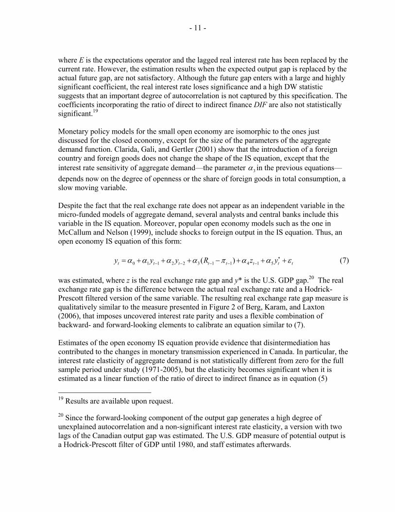
where E is the expectations operator and the lagged real interest rate has been replaced by the current rate. However, the estimation results when the expected output gap is replaced by the actual future gap, are not satisfactory. Although the future gap enters with a large and highly significant coefficient, the real interest rate loses significance and a high DW statistic suggests that an important degree of autocorrelation is not captured by this specification. The coefficients incorporating the ratio of direct to indirect finance DIF are also not statistically significant.19 Monetary policy models for the small open economy are isomorphic to the ones just discussed for the closed economy, except for the size of the parameters of the aggregate demand function. Clarida, Gali, and Gertler (2001) show that the introduction of a foreign country and foreign goods does not change the shape of the IS equation, except that the interest rate sensitivity of aggregate demand—the parameter 3α in the previous equations—depends now on the degree of openness or the share of foreign goods in total consumption, a slow moving variable. Despite the fact that the real exchange rate does not appear as an independent variable in the micro-funded models of aggregate demand, several analysts and central banks include this variable in the IS equation. Moreover, popular open economy models such as the one in McCallum and Nelson (1999), include shocks to foreign output in the IS equation. Thus, an open economy IS equation of this form: 0 1 1 2 2 3 1 1 4 1 5( )t t t t t t t ty y y R z yα α α α π α α ε∗

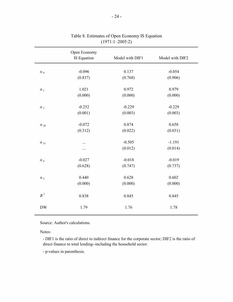
− − − − −= + + + − + + + (7) was estimated, where z is the real exchange rate gap and y* is the U.S. GDP gap.20 The real exchange rate gap is the difference between the actual real exchange rate and a Hodrick-Prescott filtered version of the same variable. The resulting real exchange rate gap measure is qualitatively similar to the measure presented in Figure 2 of Berg, Karam, and Laxton (2006), that imposes uncovered interest rate parity and uses a flexible combination of backward- and forward-looking elements to calibrate an equation similar to (7). Estimates of the open economy IS equation provide evidence that disintermediation has contributed to the changes in monetary transmission experienced in Canada. In particular, the interest rate elasticity of aggregate demand is not statistically different from zero for the full sample period under study (1971-2005), but the elasticity becomes significant when it is estimated as a linear function of the ratio of direct to indirect finance as in equation (5)

19 Results are available upon request.

20 Since the forward-looking component of the output gap generates a high degree of unexplained autocorrelation and a non-significant interest rate elasticity, a version with two lags of the Canadian output gap was estimated. The U.S. GDP measure of potential output is a Hodrick-Prescott filter of GDP until 1980, and staff estimates afterwards.

- 12 -

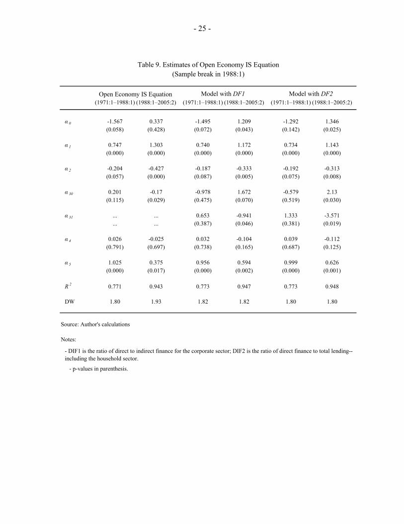
(Table 8).21 This suggests that the trends of intermediation (in the 1970s) and disintermediation (in the 1990s) might have cancelled out when they were omitted in the initial specification. Moreover, Table 9 shows that the coefficients on DIF1 and DIF2 become significant in the second half of the sample, and yield relatively larger estimates of the interest elasticity (respectively -0.46 and -048, for the average sample values of DIF1 and DIF2). This suggest that the responsiveness of aggregate demand to monetary policy actions has become stronger with the process of financial disintermediation of the 1990s.

V. CONCLUSIONS AND POLICY IMPLICATIONS

This paper shows that monetary transmission in Canada has changed markedly since the late 1980s, and also provides evidence that financial disintermediation has contributed to these changes. Estimated VAR models show a clear break in monetary transmission beginning in 1988, after changes in financial sector regulation initiated the process of financial disintermediation. Although the inclusion of financial variables in VAR models improves the characterization of monetary transmission in the period before the structural break, the models suggest a loss in the effectiveness of monetary policy in the 1990s. However, the paper presents evidence that suggests that this may be related to the fact that VAR models capture the impact of unexpected monetary shocks, while the systematic component of monetary policy—not captured in the impulse responses—has likely become more important with the improvements in the monetary framework during the 1990s. As in other industrialized countries, changes in monetary policy, the nature of global shocks, and other structural changes are likely to also have played a significant role in monetary transmission.22 The process of disintermediation has contributed to changes in the sensitivity of aggregate demand to real interest rates, a key parameter in the transmission of monetary policy to the real economy. Estimates of the interest rate elasticity of aggregate demand in IS equations increase in the 1990s, confirming the interpretation that the systematic component of monetary policy has become more relevant in the more recent period. Moreover, changes in the ratio of direct to indirect finance, a measure of disintermediation, contribute to explain the changes in the interest rate elasticity, and suggest an increased effectiveness of monetary policy associated with a larger use of market-based sources of finance in the 1990s. This could be attributed to the lower interest rate sensitivity of relationship-based bank lending compared to the more price-sensitive direct or market funding. Monetary policy appears to have become more effective in the 1990s, when measured as the average impact of interest rate changes on the output gap, or alternatively, on aggregate demand. However, this increased effectiveness may be undermined by the more recent increase in household borrowing and the relative decline in the issuance of corporate 21 When calculated using the average sample values of DIF1 and DIF2 both elasticities are respectively -0.15 and -0.09, respectively.

22 Stock and Watson (2003) estimate that for the U.S. changes in policies account for around a quarter of the reduction in volatility of the major macroeconomic aggregates.

- 13 -

securities, that lower the ratio of direct to indirect finance. As Figure 4 shows, the ratio of direct to indirect lending for the corporate sector has been declining since 2002, and the ratio to total lending has declined even more. Although the increasing role of the household sector may change monetary transmission in other ways not captured in the simple models considered in these paper, the analysis of monetary policy could benefit from a more explicit consideration of the evolving role of financial markets and intermediaries.

- 14 -

References Allen, Franklin, and Douglas Gale, 2000, Comparing Financial Systems (Cambridge,

Massachusetts: MIT Press). Atoyan, Ruben, 2005, “Econometric Investigation of Policy Preference Evolution: The Bank

of Canada Case” (unpublished; Washington: International Monetary Fund). Bean, Charles, Jens Larsen, and Kalin Nikolov, 2002, “Financial Frictions and the Monetary

Transmission Mechanism: Theory, Evidence, and Policy Implications,” ECB Working Paper No. 113 (Frankfurt: European Central Bank).

Berg, Andrew, Philippe Karam, and Douglas Laxton, 2006, “A Practical Model-Based

Approach to Monetary Policy Analysis—Overview,” IMF Working Paper forthcoming (Washington: International Monetary Fund).

Bernanke, Ben, and Mark Gertler, 1995, “Inside the Black Box: The Credit Channel of

Monetary Policy Transmission,” Journal of Economic Perspectives, Vol. 9, No. 4, pp. 27–48.

––––––and Mark Watson, 1997,“Systematic Monetary Policy and the Effect of Oil Price

Shocks,” Brookings Papers on Economic Activity, No.1, pp. 91–142. ––––––and Simon Gilchrist, 1999, “The Financial Accelerator in a Quantitative Business

Cycle Framework,” Handbook of Macroeconomics, ed. by J.B. Taylor and M. Woodford (Amsterdam: Elsevier Science).

Boivin, Jean, and Marc Giannoni, 2002, “Assessing Changes in the Monetary Transmission

Mechanism: A VAR Approach,” Federal Reserve Bank of New York Economic Policy Review, pp. 97–111.

Calmes, Christian, 2004, “Regulatory Changes and Financial Structure: The Case of

Canada,” Bank of Canada Working Paper, 2004–26, Ottawa. Cecchetti, Stephen G., “Legal Structure, Financial Structure and the Monetary Policy

Transmission Mechanism,” Federal Reserve Bank of New York Economic Policy Review, July 1999, pp. 19–28.

Clarida, Richard, Jordi Gali, and Mark Gertler, 1999, “The Science of Monetary Policy,”

Journal of Economic Literature, Vol. 37, No. 4, pp. 1661–1707. ––––––, 2001, “Optimal Monetary Policy in Open versus Closed Economies: An Integrated

Approach,” American Economic Review, Vol. 91, No. 2, pp. 248–252.

- 15 -

Christiano, Lawrence, Martin Eichenbaum, and Charles Evans, 1999, “Monetary Policy Shocks: What Have We learned and to What End?” Handbook of Macroeconomics, ed. by J.B. Taylor and M. Woodford (Amsterdam: Elsevier Science).

Estrella, Arturo, 2001, “Financial Innovation and the Monetary Transmission Mechanism,”

mimeo, Federal Reserve Bank of New York. ––––––, 2002, “Securitization and the Effectiveness of Monetary Policy,” Federal Reserve

Bank of New York Economic Policy Review. Favero, Carlo, 2001, Applied Macroeconometrics (London: Oxford University Press). Freedman, Charles, and Walter Engert, 2003, “Financial Developments in Canada: Past

Trends and Future Challenges,” Bank of Canada Review, Summer, p. 3–16. Fung, Ben S.C., and Mingwei Yuan, 1999, “Measuring the Stance of Monetary Policy,” in

Money, Monetary Policy and Transmission Mechanisms—Proceedings of a Conference held at the Bank of Canada.

Kashyap, Anil K., and Jeremy C. Stein, 1994, “Monetary Policy and bank Lending”,

Monetary Policy, NBER Studies in Business Cycles, ed. by N. Gregory Mankiw, Vol. 29, pp. 221–61 (Chicago: University of Chicago Press).

Levin, Andrew T., Fabio Natalucci and Egon Zakrajsek, 2004, “The Magnitude and Cyclical

Behavior of Financial Market Frictions,” Finance and Economic Discussion Series, 2004-70, Federal Reserve Board, Washington D.C.

McCallum, Bennett, and Edward Nelson, 1999, “Nominal Income Targeting in an Open-

Economy Optimizing Model,” Journal of Monetary Economics, 43, pp. 553–78. Morsink, James, and Tamim Bayoumi, 2001, “A Peek Inside the Black Box: The Monetary

Transmission Mechanism in Japan”, IMF Staff Papers, Vol. 48, No. 1, pp. 22–57. Peersman, Gert, and Frank Smets, 2001, “The Monetary Transmission Mechanism in the

Euro Area: More Evidence from VAR Analysis,” European Central Bank WP No. 91. Rudebusch, Glenn D., and Lars E. O. Svensson, 1999, “Policy Rules for Inflation Targeting,”

Monetary Policy Rules, ed. by John B. Taylor (Chicago: University of Chicago Press).

Stock, James H., and Mark W. Watson, 2003, “Has the Business Cycle Changed and Why?,”

in NBER Macro Annual 2000, ed. by M. Gertler and K. Rogoff (Cambridge Massachussets: MIT Press).

- 16 -

Stock, James H., and Mark W. Watson, 2005, “Understanding Changes in International Business Cycle Dynamics,” Journal of the European Economic Association, Vol. 3, No.5, pp. 968–1006.

- 17 -

EquationGDP 1.777 * 2.008 * 2.217 * 2.221 * 2.233 *Prices 1.118 1.296 1.004 2.094 * 1.892 *Ints. Rate 1.755 * 1.953 * 1.436 1.565 1.836 *Exch.Rate 1.894 * 2.024 * 2.582 * 3.135 * 3.116 *Loans ... 3.751 * ... ... 4.069 *CP-Spread ... ... 1.275 ... ...Asset Prices ... ... ... 1.972 * 1.636 *

LR-Test 293.0 433.0 498.3 424.7 606.4

Table 1. Canada: Tests for Break in VAR Model in 1988:1(F-Statistics; 1971:1–1988:1; 1988:1–2005:2)

CP-SpreadsLoans

BenchmarkLoans &

Asset PricesAsset

Financial

The unrestricted model is the one that has different parameters for the two subsamples; the restricted one imposes equality across the subsamples. The LR tests the statistical significance of these restrictions, and is distributed Chi-square with degree of freedom equal to the number of restrictions (100 for the benchmark model, 120 for the financial models); the Chi-square values for 120 degrees of freedom are 146.6 (5%) and 159.0 (1%) respectively.The F-test statistics are the corresponding single equation test statistics; they are, however, not distributed as F here because of the presence of lagged dependent variables. The F(24, 80) value for 5 percent significance is 1.65.

Notes:

Prices

- 18 -

EquationGDP 1.487 1.859 * 1.355 1.479 2.214 *Prices 1.853 * 2.418 * 1.825 * 2.197 * 2.193 *Ints. Rate 1.114 0.929 1.179 0.959 0.637Exch. Rate 1.567 1.699 * 1.431 1.739 * 2.237 *Loans ... 3.060 * ... ... 2.896 *CP-Spread ... ... 1.072 ... ...Asset Prices ... ... ... 1.406 1.237

LR-Test 328.5 445.8 489.3 416.8 609.6


Benchmark FinancialAsset Loans &

Loans CP-Spreads Prices Asset Prices

Notes:The unrestricted model is the one that has different parameters for the two subsamples; the restricted one imposes equality across the subsamples. The LR tests the statistical significance of these restrictions, and is distributed Chi-square with degree of freedom equal to the number of restrictions (100 for the benchmark model, 120 for the financial models); the Chi-square values for 120 degrees of freedom are 146.6 (5%) and 159.0 (1%) respectively.The F-test statistics are the corresponding single equation test statistics; they are, however, not distributed as F here because of the presence of lagged dependent variables. The F(24, 80) value for 5 percent significance is 1.65.

- 19 -

BenchmarkLoans &

Loans CP-Spreads Asset Prices Asset Prices

EquationGDP 1.276 1.615 1.239 1.406 1.946Prices 1.876 2.375 1.990 2.39 2.341Ints. Rate 1.500 1.186 1.028 0.952 1.038Exch.Rate 1.580 1.810 1.505 1.944 2.137Loans ... 4.114 ... ... 4.479CP-Spread ... ... 1.110 ... ...Asset Prices ... ... ... 1.482 1.240

LR-Test 284.2 430.1 447.0 366.1 560.2

Notes:

The unrestricted model is the one that has different parameters for the two subsamples; the restricted one imposes equality across the subsamples. The LR tests the statistical significance of these restrictions, and is distributed Chi-square with degree of freedom equal to the number of restrictions (100 for the benchmark model, 120 for the financial models); the Chi-square values for 120 degrees of freedom are 146.6 (5%) and 159.0 (1%) respectively.

The F-test statistics are the corresponding single equation test statistics; they are, however, not distributed as F here because of the presence of lagged dependent variables. The F(24, 80) value for 5 percent significance is 1.65.


Financial

- 20 -

Table 4. Canada: Variance Decompositions of GDP to Monetary Shock

(in percent)

Baseline Model

Quarter Full Sample 1971-1991 1991-2005

4 0.8 1.6 1.38 9.2 20.4 1.1

12 15.6 27.1 1.216 15.9 26.9 1.2

Model with Loans


4 1.6 0.6 9.18 9.8 22.7 8.7

12 14.5 33.7 9.216 15.5 32.1 9.2

Model with Asset Prices


4 1.2 2.1 2.48 8.7 22.8 2.0

12 16.2 35.3 3.716 18.7 34.6 4.2

Model with Loans and Asset Prices


4 1.4 0.5 4.58 9.8 25.0 3.3

12 16.7 39.6 3.216 19.2 35.1 4

Source: Author's calculations.

- 21 -

Table 5. Canada: Changes in the Standard Deviations of Shocks

(Interest Rate Equation)

Model 1971–1991 1991–2005 SD2/SD1

Baseline VAR 0.49 0.41 0.84

VAR with Loans 0.49 0.46 0.94

VAR with Asset Prices 0.52 0.44 0.85

VAR with Loans and Asset Prices 0.49 0.44 0.90


Note: The last column shows the ratio of the standard deviation of the monetary shock in the second and first subsamples.

- 22 -

Table 6. Canada: Estimates of Closed Economy IS Equation

(1971:1–2005:2)

Closed Economy IS Equation Model with DIF1 Model with DIF2

α 0 0.473 0.483 0.476(0.300) (0.325) (0.309)

α 1 1.141 1.141 1.141(0.000) (0.000) (0.000)

α 2 -0.298 -0.298 -0.298(0.000) (0.000) (0.000)

α 30 -0.156 -0.137 -0.147(0.029) (0.684) (0.592)

α 31 ... -0.010 -0.015... (0.954) (0.974)

R 2 0.818 0.818 0.818

DW 2.00 2.00 2.00

Source: Author's calculations

Notes: - DIF1 is the ratio of direct to indirect finance for the corporate sector; DIF2 is the ratio

- p-values in parenthesis.

of direct finance to total lending--including the household sector.

- 23 -

Table 7. Canada: Estimates of Closed Economy IS Equation

(Sample break in 1988:1)

Model with DIF1 Model with DIF2(1971:1–1988:1) (1988:1–2005:2) (1971:1–1988:1) (1988:1–2005:2) (1971:1–1988:1) (1988:1–2005:2)

α 0 0.216 0.437 0.024 0.565 0.723 0.656(0.792) (0.314) (0.976) (0.355) (0.392) (0.265)

α 1 1.029 1.425 0.971 1.418 0.976 1.411(0.000) (0.000) (0.000) (0.000) (0.000) (0.000)

α 2 -0.273 -0.511 -0.225 -5.507 -0.244 -0.503(0.027) (0.000) (0.064) (0.000) (0.044) (0.000)

α 30 -0.143 -0.130 -3.079 0.094 -1.971 0.322(0.208) (0.089) (0.032) (0.900) (0.044) (0.693)

α 31 ... ... 1.661 -0.114 3.158 -0.700... ... (0.040) -0.765 (0.059) (0.578)

R 2 0.687 0.938 0.708 0.938 0.704 0.938

DW 1.98 2.04 2.00 2.03 1.96 2.02

Notes:

Benchmark IS Equation


- DIF1 is the ratio of direct to indirect finance for the corporate sector; DIF2 is the ratio of direct finance to total lending--including the household sector.

- 24 -

Table 8. Estimates of Open Economy IS Equation

(1971:1–2005:2)

Open EconomyIS Equation Model with DIF1 Model with DIF2

α 0 -0.096 0.137 -0.054(0.837) (0.768) (0.906)

α 1 1.021 0.972 0.979(0.000) (0.000) (0.000)

α 2 -0.252 -0.229 -0.229(0.001) (0.003) (0.003)

α 30 -0.072 0.874 0.658(0.312) (0.022) (0.031)

α 31 ... -0.505 -1.191... (0.012) (0.014)

α 4 -0.027 -0.018 -0.019(0.628) (0.747) (0.737)

α 5 0.440 0.628 0.602(0.000) (0.000) (0.000)

R 2 0.838 0.845 0.845

DW 1.79 1.76 1.78


Notes:



- 25 -

Table 9. Estimates of Open Economy IS Equation

(Sample break in 1988:1)

Open Economy IS Equation Model with DF1 Model with DF2(1971:1–1988:1) (1988:1–2005:2) (1971:1–1988:1) (1988:1–2005:2) (1971:1–1988:1) (1988:1–2005:2)

α 0 -1.567 0.337 -1.495 1.209 -1.292 1.346(0.058) (0.428) (0.072) (0.043) (0.142) (0.025)

α 1 0.747 1.303 0.740 1.172 0.734 1.143(0.000) (0.000) (0.000) (0.000) (0.000) (0.000)

α 2 -0.204 -0.427 -0.187 -0.333 -0.192 -0.313(0.057) (0.000) (0.087) (0.005) (0.075) (0.008)

α 30 0.201 -0.17 -0.978 1.672 -0.579 2.13(0.115) (0.029) (0.475) (0.070) (0.519) (0.030)

α 31 ... ... 0.653 -0.941 1.333 -3.571... ... (0.387) (0.046) (0.381) (0.019)

α 4 0.026 -0.025 0.032 -0.104 0.039 -0.112(0.791) (0.697) (0.738) (0.165) (0.687) (0.125)

α 5 1.025 0.375 0.956 0.594 0.999 0.626(0.000) (0.017) (0.000) (0.002) (0.000) (0.001)

R 2 0.771 0.943 0.773 0.947 0.773 0.948

DW 1.80 1.93 1.82 1.82 1.80 1.80

Source: Author's calculations

Notes:



- 26 -

Source: Bank of Canada.

Loans

Equities

Other

0

20

40

60

80

100

1971 1975 1979 1983 1987 1991 1995 1999 2003

0

20

40

60

80

100

Bonds, debentures, and short-term

paper

Figure 1. Nonfinancial Corporate Financing Sources, 1971–2005(stocks outstanding, in percent of total)

- 27 -

Figure 2. Credit Flows, 1971–2005

Source: Bank of Canada

-10

-5

0

5

10

15

1971 1975 1979 1983 1987 1991 1995 1999 2003

-10

-5

0

5

10

15

Bonds and debentures

Credit Flows, 1971–2005 (billion Canadian dollars)

Loans

Commercial paper

-10

-5

0

5

10

15

1991 1993 1995 1997 1999 2001 2003 2005

-10

-5

0

5

10

15

Bonds and debentures

Credit Flows, 1991–2005 (billion Canadian dollars)

Loans

Commercial paper

- 28 -


0.0

0.2

0.4

0.6

0.8

1.0

1971 1975 1979 1983 1987 1991 1995 1999 2003

0.0

0.2

0.4

0.6

0.8

1.0

Figure 3. Ratio of Direct to Indirect Private Lending, 1971–2005

- 29 -


0

100

200

300

400

500

600

700

1971 1975 1979 1983 1987 1991 1995 1999 2003

0

100

200

300

400

500

600

700

Household mortgages

Figure 4. Outstanding Credit, 1971–2005 (billion Canadian dollars)

Business loans

Consumer credit

- 30 -

Figure 5. Canada: Impulse-Response Functions from Benchmark VAR

Source: Fund staff calculations.

-.004

-.003

-.002

-.001

.000

.001

.002

.003

.004

2 4 6 8 10 12 14 16 18 20

Response of GDP_R to TBILL3MO

-.003

-.002

-.001

.000

.001

.002

.003

2 4 6 8 10 12 14 16 18 20

Response of GDP_P to TBILL3MO

-.6

-.4

-.2

.0

.2

.4

.6

.8

2 4 6 8 10 12 14 16 18 20

Response of TBILL3MO to TBILL3MO

-2

-1

0

1

2

3

2 4 6 8 10 12 14 16 18 20

Response of XR_INDEX_LEV to TBILL3MO

Full sample 1971-Q1 to 1991-Q1 1991-Q1 to 2005-Q2

-.003

-.002

-.001

.000

.001

.002

.003

.004

2 4 6 8 10 12 14 16 18 20


-.003

-.002

-.001

.000

.001

.002

.003

2 4 6 8 10 12 14 16 18 20


-.6

-.4

-.2

.0

.2

.4

.6

.8

2 4 6 8 10 12 14 16 18 20


-2

-1

0

1

2

3

2 4 6 8 10 12 14 16 18 20


-.002

-.001

.000

.001

.002

.003

2 4 6 8 10 12 14 16 18 20


-.0010

-.0005

.0000

.0005

.0010

.0015

.0020

2 4 6 8 10 12 14 16 18 20


-.4

-.2

.0

.2

.4

.6

.8

2 4 6 8 10 12 14 16 18 20


-2

-1

0

1

2

3

2 4 6 8 10 12 14 16 18 20


- 31 -

Figure 6. Canada: Impulse-Response Functions from VAR including Business Loans



-.004

-.003

-.002

-.001

.000

.001

.002

.003

.004

2 4 6 8 10 12 14 16 18 20


-.003

-.002

-.001

.000

.001

.002

.003

2 4 6 8 10 12 14 16 18 20


-.6

-.4

-.2

.0

.2

.4

.6

.8

2 4 6 8 10 12 14 16 18 20


-0.8

-0.4

0.0

0.4

0.8

1.2

1.6

2.0

2.4

2.8

2 4 6 8 10 12 14 16 18 20


-.003

-.002

-.001

.000

.001

.002

.003

.004

2 4 6 8 10 12 14 16 18 20


-.003

-.002

-.001

.000

.001

.002

.003

2 4 6 8 10 12 14 16 18 20


-.6

-.4

-.2

.0

.2

.4

.6

.8

2 4 6 8 10 12 14 16 18 20


-1.2

-0.8

-0.4

0.0

0.4

0.8

1.2

1.6

2.0

2.4

2 4 6 8 10 12 14 16 18 20


-.001

.000

.001

.002

2 4 6 8 10 12 14 16 18 20


-.0010

-.0005

.0000

.0005

.0010

.0015

.0020

2 4 6 8 10 12 14 16 18 20


-.4

-.2

.0

.2

.4

.6

.8

2 4 6 8 10 12 14 16 18 20


-1

0

1

2

2 4 6 8 10 12 14 16 18 20


- 32 -

Figure 7. Canada: Impulse-Response Functions from VAR including Asset Prices



-.004

-.003

-.002

-.001

.000

.001

.002

.003

.004

2 4 6 8 10 12 14 16 18 20


-.003

-.002

-.001

.000

.001

.002

.003

2 4 6 8 10 12 14 16 18 20


-.6

-.4

-.2

.0

.2

.4

.6

.8

2 4 6 8 10 12 14 16 18 20


-1.0

-0.5

0.0

0.5

1.0

1.5

2.0

2.5

2 4 6 8 10 12 14 16 18 20


-.003

-.002

-.001

.000

.001

.002

.003

.004

2 4 6 8 10 12 14 16 18 20


-.003

-.002

-.001

.000

.001

.002

.003

2 4 6 8 10 12 14 16 18 20


-.6

-.4

-.2

.0

.2

.4

.6

.8

2 4 6 8 10 12 14 16 18 20


-2

-1

0

1

2

3

2 4 6 8 10 12 14 16 18 20


-.001

.000

.001

.002

2 4 6 8 10 12 14 16 18 20


-.0010

-.0005

.0000

.0005

.0010

.0015

.0020

2 4 6 8 10 12 14 16 18 20


-.4

-.2

.0

.2

.4

.6

.8

2 4 6 8 10 12 14 16 18 20


-2

-1

0

1

2

2 4 6 8 10 12 14 16 18 20


- 33 -

Figure 8. Canada: Impulse-Response Functions from VAR including Asset Prices and Business Loans



-.003

-.002

-.001

.000

.001

.002

.003

.004

2 4 6 8 10 12 14 16 18 20


-.003

-.002

-.001

.000

.001

.002

.003

2 4 6 8 10 12 14 16 18 20


-.6

-.4

-.2

.0

.2

.4

.6

.8

2 4 6 8 10 12 14 16 18 20


-2

-1

0

1

2

3

2 4 6 8 10 12 14 16 18 20


-.003

-.002

-.001

.000

.001

.002

.003

.004

2 4 6 8 10 12 14 16 18 20


-.003

-.002

-.001

.000

.001

.002

.003

2 4 6 8 10 12 14 16 18 20


-.6

-.4

-.2

.0

.2

.4

.6

.8

2 4 6 8 10 12 14 16 18 20


-1.0

-0.5

0.0

0.5

1.0

1.5

2.0

2.5

2 4 6 8 10 12 14 16 18 20


-.0015

-.0010

-.0005

.0000

.0005

.0010

.0015

.0020

2 4 6 8 10 12 14 16 18 20


-.0015

-.0010

-.0005

.0000

.0005

.0010

.0015

.0020

2 4 6 8 10 12 14 16 18 20


-.4

-.2

.0

.2

.4

.6

.8

2 4 6 8 10 12 14 16 18 20


-2

-1

0

1

2

2 4 6 8 10 12 14 16 18 20


Documents

Disintermediation and Monetary Transmission in Canada