Embed Size (px)
Citation preview

Mediterranean Sea Hydrographic Atlas: towards optimal dataanalysis by including time-dependent statistical parametersAthanasia Iona1,2, Athanasios Theodorou2, Sylvain Watelet3, Charles Troupin3, and Jean-Marie Beckers3
1Hellenic Centre for Marine Research, Institute of Oceanography, Hellenic National Oceanographic Data Centre, 46,7 kmAthens Sounio, Mavro Lithari P.O. BOX 712 19013 Anavissos, Attica, Greece2University of Thessaly, Department of Ichthyology & Aquatic Environment, Laboratory of Oceanography, Fytoko Street, 38445, Nea Ionia Magnesia, Greece3University of Liège, GeoHydrodynamics and Environment Research, Quartier Agora, Allée du 6-Août, 17, Sart Tilman,4000 Liège 1, Belgium
Correspondence: Athanasia Iona ([email protected])
Abstract. The goal of the present work is to provide the scientific community with a high-resolution Atlas of temperature and
salinity for the Mediterranean Sea based on the most recent datasets available and contribute to the studies of the long-term
variability in the region. Data from the Pan-European Marine Data Infrastructure SeaDataNet were used, the most complete
and, to our best knowledge, of best quality dataset for the Mediterranean Sea as of today. The dataset is based on in situ mea-
surements acquired between 1900–2015. The Atlas consists of horizontal gridded fields produced by the Data Interpolating5
Variational Analysis, where unevenly spatial distributed measurements were interpolated onto a 1/8◦ × 1/8◦ regular grid on 31
depth levels. Seven different types of climatological fields were prepared with different temporal integration of observations.
Monthly, seasonal and annual climatological fields have been calculated for all the available years, seasonal to annual clima-
tologies for overlapping decades and specific periods. The seasonal and decadal time frames have been chosen in accordance
with the regional variability and in coherence with atmospheric indices. The decadal and specific periods analysis was not10
extended to monthly resolution due to the lack of data, especially for the salinity. The Data Interpolating Variational Analysis
software has been used in the Mediterranean Region for the SeaDataNet and its predecessor Medar/Medatlas Climatologies. In
the present study, a more advanced optimization of the analysis parameters was performed in order to produce more detailed
results. The Mediterranean Region past and present states have been extensively studied and documented in a series of publica-
tions. The purpose of this Atlas is to contribute to these climatological studies and get a better understanding of the variability15
on time scales from month to decades and longer. Our gridded fields provide a valuable complementary source of knowledge in
regions where measurements are scarce, especially in critical areas of interest such as the Marine Strategy Framework Directive
(MSFD) regions. The dataset used for the preparation of the Atlas is available from https://doi.org/10.12770/8c3bd19b-9687-
429c-a232-48b10478581c.
1
Earth Syst. Sci. Data Discuss., https://doi.org/10.5194/essd-2018-9
Ope
n A
cces
s Earth System
Science
DataD
iscussio
ns
Manuscript under review for journal Earth Syst. Sci. DataDiscussion started: 2 February 2018c© Author(s) 2018. CC BY 4.0 License.

1 Introduction
In oceanography, a climatology is defined as a set of gridded fields that describe the mean state of the ocean properties over a
given time period. It is constructed by the analysis of in-situ historical data sets and has many applications such as initialization
of numerical models, quality control of observational data in real time and delayed mode, and it is used as a baseline for
comparison to understand how the ocean is changing. The Mediterranean Sea is among the most interesting regions in the world5
because it influences the global thermohaline circulation and plays an important role in regulating the global climate (Lozier
et al., 1995; Béthoux et al., 1998; Rahmstorf, 1998). It is therefore essential to improve our understanding of its dynamics and its
process variability. It is a semi-enclosed sea divided by the Sicily Strait in two geographical basins: the Western Mediterranean
and the Eastern Mediterranean and characterized by peculiar topographic deep depressions where nutrient-rich deep-water
masses are stored for long time (Manca et al., 2004). It is a concentration basin, where evaporation exceeds precipitation. The10
general mean circulation pattern is driven by the continuous evaporation, heat fluxes exchanges with the atmosphere, the wind
stress and the water masses exchanges between its basins and sub basins, as described in Robinson et al. (2001). In the surface
layer (0–150 m) there is an inflow of warm and relatively fresh Atlantic water (AW; S ≈ 36.5, T ≈ 15◦C) which is modified
along its path to the Eastern basin following a general cyclonic circulation. The intermediate layers (150–600 m) are dominated
by the saline Levantine Intermediate Water (LIW; S ≈ 38.4, T ≈ 13.5◦C), regularly formed at the Levantine basin. LIW is15
one of the most important Mediterranean water masses because it constitutes the higher percentage of the outflow from the
Gibraltar Strait towards the Atlantic Ocean. In the deep layers, there are two main thermohaline cells. Deep waters formed via
convective events in the northern regions of the Western Mediterranean (WMDW-Western Mediterranean Deep Water; S ≈38.44–38.46, T ≈ 12.75–13.80◦C) at the Gulf of Lions and at the north regions of the Eastern Mediterranean (EMDW-Eastern
Mediterranean Deep Waters) at the Adriatic (S ≈ 38.65, T ≈ 13.0◦C) and Cretan Sea (σθ < 29.2). On top of this large scale20
general pattern are superimposed several sub-basin scale and mesoscale cyclonic and anticyclonic motions due to topographic
constraints and internal processes. The first climatological studies of the Mediterranean go back to 1966 with Ovchinnikov
who carried out a geostrophic analysis to compute the surface circulation. The circulation features were describing a linear,
stationary ocean. In the 1980s and 1990s, through a comprehensive series of observational studies and experiments in the
Western Mediterranean (La Violette, 1990; Millot, 1987, 1991, 1999), the sub-basin and mesoscale patterns were discovered25
and the crucial role of eddies in modifying the mean climatological circulation and mixing properties inside the different sub-
basins which include the Tyrrhenian, Ligurian and Alboran Seas was emphasized (Bergamasco and Malanotte-Rizzoli, 2010).
In 1987, Guibout constructed charts with the typical structures observed at sea, but with limited climatological characteristic as
this atlas was based on the quasi-synoptic information of the selected cruise used. In 1982, an international research group was
formed, called POEM (Physical Oceanography of the Eastern Mediterranean, 1984), under the auspices of the IOC/UNESCO30
and of CIESM (Commission Internationale pour l’Exploration Scientifique de la Méditerranée) focused on the description
of the phenomenology of the Eastern Mediterranean, by analysing historical data and collecting new data (Malanotte-Rizzoli
and Hecht, 1988). However the focus was on the Eastern Mediterranean Sea, as there was very little knowledge of this basin
compared to the Western Mediterranean and other world regions and still there was missing a global data set to describe the
2
Earth Syst. Sci. Data Discuss., https://doi.org/10.5194/essd-2018-9
Ope
n A
cces
s Earth System
Science
DataD
iscussio
ns
Manuscript under review for journal Earth Syst. Sci. DataDiscussion started: 2 February 2018c© Author(s) 2018. CC BY 4.0 License.

eastern Mediterranean efficiently and its interaction with the western part. Hecht et al. (1988), by analyzing hydrographic
measurements in the south eastern Levantine Basin, succeeded to describe the climatological water masses of the region and
identify their seasonal variations. In the western Mediterranean, Picco (1990) conducted an important climatological study and
constructed a climatological atlas analyzing around 15000 hydrological profiles from various sources for the period 1909–
1987. In 1982, Levitus published the first climatological atlas of the world ocean at a 1◦ resolution, using temperature, salinity5
and oxygen data from CTD, Bottle stations, mechanical and expendable bathythermographs of the previous eighty years. An
objective analysis at standard levels was followed to compute the climatology. Since 1994, a new version is released every 4
years. The current version that includes the Mediterranean (World Ocean Atlas 2013, V2) (Locarnini et al., 2013) is a long-term
set of objectively analyzed climatologies of temperature, salinity, oxygen, phosphate, silicate, and nitrate for annual, seasonal,
and monthly periods for the world ocean. It also includes associated statistical fields of observed oceanographic profile data10
from which the climatologies were computed. In addition to increased vertical resolution, the 2013 version has both 1◦ and 1/4◦
horizontal resolution versions available for annual and seasonal temperature and salinity for six decades, as well as monthly
for the decadal average. Brasseur et al. (1996) introduced a new method to reconstruct the three-dimensional fields of the
properties of the Mediterranean Sea. Seasonal and monthly fields were analyzed using a Variational Inverse Method (VIM) to
generate the climatological maps, instead of the objective analysis introduced by Gandin (1966); Bretherton et al. (1976) to15
the meteorology and oceanography and widely used by then. More than 34000 CTD and Bottle data were used and integrated
in the so-called MED2 historical data base. Comparison of the results obtained with both methods showed that VIM was
mathematically equivalent but numerically more efficient than the objective analysis. The method has been adopted by the
Medar/Medatlas and its successor SeaDataNet Project.
At the beginning of the 2000s, many research projects and monitoring activities have produced large amounts of multidis-20
ciplinary in-situ hydrographic and bio-chemical data for the whole Mediterranean Sea but still the data were fragmented and
inaccessible from the scientific community. The aim of the EU/MAST Medar/Medatlas Project, 2001 (http://www.ifremer.fr/
medar/) was to rescue and archive the dispersed data through a wide cooperation of countries and produce an atlas for 12
core parameters: temperature and salinity, dissolved oxygen, hydrogen sulphur, alkalinity, phosphate, ammonium, nitrite, ni-
trate, silicate, chlorophyll and PH. Gridded fields have been computed on a 1/4◦ grid resolution using the Variational Inverse25
Method (VIM) and the DIVA tool developed by the GHER group of the University of Liège. Inter-annual and decadal vari-
abilities of temperature and salinity were computed as well. The atlas is available at http://modb.oce.ulg.ac.be/backup/medar/
contribution.html and on CD-Rom (MEDAR Group, 2002). The atlas contains a selection of figures and 3D fields in netCDF.
The EU/FP7 SeaDataNet Project 2006-2011, 2012-2016 (the successor of the EU/MAST Medar/Medatlas) has integrated
historical, multidisciplinary data on a unique, standardized online data management infrastructure and provides value-added30
aggregated datasets and regional climatologies based on these aggregated datasets for all the European sea basins. SeaDataNet
has adopted the VIM method and the DIVA software tool. Temperature and salinity monthly climatologies have been produced
on a 1/8◦ grid resolution. These climatologies are based on the V1.1 historical data collection of publicly available temperature
and salinity in situ profiles (http://dx.doi.org/10.12770/8c3bd19b-9687-429c-a232-48b10478581c) spanning the time period
1900-2013 (Simoncelli et al., 2015).
3
Earth Syst. Sci. Data Discuss., https://doi.org/10.5194/essd-2018-9
Ope
n A
cces
s Earth System
Science
DataD
iscussio
ns
Manuscript under review for journal Earth Syst. Sci. DataDiscussion started: 2 February 2018c© Author(s) 2018. CC BY 4.0 License.
1.1 Objectives
The objective of this study is the computation of an improved Atlas compared with the existing products in the Mediterranean
Sea using the latest developments of the DIVA tool with the aim to contribute to the better representation of the climatological
patterns and understanding of the long-term variability of the regional features of the basin. The originality of this product com-5
pared to the SeaDataNet climatology (both products use similar techniques) is the higher temporal resolution, up to decadal,
and more advanced calibration of the analysis parameters for improving the results and the representation of general circulation
patterns at time scales smaller than the climatic means. Besides the WOA13 decadal periods climatologies (1955–64, 1965–
74, 1975–84, 1985–94, 1995–2004 and 2005–2012) the Medar/Medatlas provides interannual and decadal gridded fields and
therefore it is compared with the present Atlas. The present product has two major improvements: higher spatial and vertical10
resolution and error fields that accompany all the analysis results, allowing therefore a more reliable assessment of the results.
The advantage of this product in relation to the WOA13 climatology is the higher spatial resolution up to 1/8◦ × 1/8◦ longi-
tude/latitude grids used and the higher temporal resolution as the analysis uses running decades instead of successive decades.
Another important difference with respect to all previous existing climatologies in the Mediterranean is that additional and
more recent data are used. The Atlas constructed consists of climatological fields (called climatology hereafter) to depict the15
“mean” state of the Mediterranean region at monthly, seasonal: winter (Jan–Mar), spring (Apr–Jun), summer (Jul–Sep), fall
(Oct–Dec), and annual scale. Additionally, climatological fields at seasonal and annual scale for 57 running decades have been
produced to depict the interannual and decadal variability of the system and reveal the decadal trends.
One additional period from 2000–2015 was produced for those users or applications who are interested to reference to the
latest data and new platform types such as Argo floats. This period is provided with the five previous successive decadal periods20
e.g. 1950–1959, 1960–1969, 1970–1979, 1980–1989, 1990–1999 and 2000–2015. In summary, the following gridded products
are available:
– Monthly climatological gridded fields obtained by analyzing all data of the whole period 1950 to 2015 falling within
each month.
– Seasonal climatological gridded obtained by analyzing all data of the whole period from 1950 to 2015 falling within25
each season.
– Seasonal gridded fields obtained by analyzing all data falling within each season for each of 57 running decade from
1950–1959 to 2006–2015.
– Seasonal gridded fields obtained by analyzing data falling within each season for six periods: 1950–1959, 1960–1969,
1970–1979, 1980–1989, 1990–1999, 2000–2015.30
– Annual climatology obtained by analyzing all data (regardless month or season) for the whole period from 1950 to 2015.
– Annual gridded fields by analyzing all data regardless month or season for each of the 57 running decade from 1950–
1959 to 2006–2015.
4
Earth Syst. Sci. Data Discuss., https://doi.org/10.5194/essd-2018-9
Ope
n A
cces
s Earth System
Science
DataD
iscussio
ns
Manuscript under review for journal Earth Syst. Sci. DataDiscussion started: 2 February 2018c© Author(s) 2018. CC BY 4.0 License.

– Annual gridded fields obtained by analyzing data falling with each season for six periods, 1950–1959, 1960–1969,
1970–1979, 1980–1989-1990–1999, 2000–2015. The first five periods coincide with the corresponding decades.
The Atlas covers the geographical region -6.25◦W–36.5◦E, 30◦–46◦N on 31 standard depth levels from 0–4000m. The fields5
are stored in netCDF files. The Atlas is accessible in netCDF from the Zenodo platform using the following DOIs:
Annual Climatology: https://doi.org/10.5281/zenodo.1146976.
Seasonal Climatology for 57 running decades from 1950-1959 to 2006-2015:
https://doi.org/10.5281/zenodo.1146938.
Seasonal Climatology: https://doi.org/10.5281/zenodo.1146953.10
Annual Climatology for 57 running decades from 1950-1959 to 2006-2015:
https://doi.org/10.5281/zenodo.1146957.
Seasonal Climatology for six periods: 1950-1959, 1960-1969, 1970-1979, 1980-1989, 1990-1999, 2000-2015:
https://doi.org/10.5281/zenodo.1146966.
Annual Climatology for six periods: 1950-1959, 1960-1969, 1970-1979, 1980-1989, 1990-1999, 2000-2015:15
https://doi.org/10.5281/zenodo.1146970.
Monthly Climatology: https://doi.org/10.5281/zenodo.1146974.
Tables 1 and 2 give the state of the art of the existing climatologies in the Mediterranean Sea.
2 Data
2.1 Data source20
The SeaDataNet Temperature and Salinity historical data collection V2 for the Mediterranean Sea was used (INVG, 2015,
http://sextant.ifremer.fr/record/8c3bd19b-9687-429c-a232-48b10478581c/). The collection includes 213542 temperature and
138691 salinity profiles from in-situ measurements covering the 1911–2015 period, which corresponds to all open access data
available through the European SeaDataNet Marine Data Infrastructure (www.seadatanet.org). These datasets were collected
from 102 data providers, are quality controlled and archived in 32 marine and oceanographic data centres and distributed into25
the infrastructure by 27 SeaDataNet partners. The data range from 9.25◦W to 37◦E and include a part of the Atlantic (not
included in the Atlas) and the Marmara Sea. Figure 1 shows the locations of the profiles and Table 3 the main instruments of
the collection.
The profiles in the SeaDataNet collection come from in-situ observations collected with various instruments and platforms
such as CTD and Bottles data by discrete water samplers operated by research or other smaller vessels, bathythermographs
5
Earth Syst. Sci. Data Discuss., https://doi.org/10.5194/essd-2018-9
Ope
n A
cces
s Earth System
Science
DataD
iscussio
ns
Manuscript under review for journal Earth Syst. Sci. DataDiscussion started: 2 February 2018c© Author(s) 2018. CC BY 4.0 License.

Table 1. Overview of characteristics of existing T/S climatologies in Mediterranean Sea.
Climatology World Ocean Atlas
2013
Medar/Medatlas SeaDataNet Present
Date 2013 2002 2015 2017
Instruments/platforms Bathythermographs,
discrete water sam-
plers, CTD, drifters,
profiling floats, gliders
Bathythermographs,
discrete water sam-
plers, CTD, thermistor
chains
Bathythermographs,
discrete water sam-
plers, CTD, thermistor
chains, thermos-
alinographs, drifters,
profiling floats, moor-
ings
Bathythermographs,
discrete water sam-
plers, CTD, thermistor
chains, thermos-
alinographs, drifters,
profiling floats, moor-
ings
Horizontal extent Global Mediterranean, Black
Sea
Mediterranean Sea Mediterranean Sea
Parameters Temperature, salinity Temperature, salinity,
bio-chemical parame-
ters
Temperature, salinity Temperature, salinity
Horizontal resolution 1/4◦ × 1/4◦ 1/4◦ × 1/4◦ 1/8◦ × 1/8◦ 1/8◦ × 1/8◦
Vertical extent 0–1500 m 0–4000 m 0–5500 m 0–5500 m
Vertical levels 57 25 33 33
Temporal data cover-
age
1864–2013 1890–2000 1900–2013 1900–2015
Temporal resolution Climatic, monthly, sea-
sonal, averaged periods
Climatic, monthly,
seasonal, inter-annual*,
running 3-years*, run-
ning 5-years, running
decades*
Monthly Climatic, monthly, sea-
sonal, running decades,
averaged periods
No error fields are available for the Medar/Medatlas, inter-annual*, running 3-years* and running decades* computations.
(mechanical or expendable). Table 3 summarizes the major numbers for temperature and salinity profiles and their temporal
spanning as derived from the station type, the instrument and the platform type.
There are 21682 vertical profiles of Temperature and Salinity from CTD and Bottle stations with no information on the5
instrument used. These figures correspond to profiles before the quality control and the processing of data for preparation of
climatology.
The Bathythermographs data were maintained in the collection despite the incorrect fall rate and the resulting warm bias in
the measurements (Wijffels et al., 2008). Yet, there is not a XBT/MBT correction for the Mediterranean as for the global ocean
(https://www.nodc.noaa.gov/OC5/XBT_BIAS/xbt_bias.html). These data improve significantly the geographical coverage of
6
Earth Syst. Sci. Data Discuss., https://doi.org/10.5194/essd-2018-9
Ope
n A
cces
s Earth System
Science
DataD
iscussio
ns
Manuscript under review for journal Earth Syst. Sci. DataDiscussion started: 2 February 2018c© Author(s) 2018. CC BY 4.0 License.

Table 2. Analysis parameters for Variational Inverse Method (VIM) implementation in the Mediterranean.
Climatology Medar/Medatlas SeaDataNet Present
Method VIM DIVA (VIM) DIVA (VIM)
Correlation length constant constant variable
Signal-to-noise ratio variable constant variable
Background field semi-normed semi-normed semi-normed
Detrending No No Yes (for background fields)
Observation weighting No No Yes
(a) Temperature
(b) Salinity
Figure 1. Geographical distribution of (a) temperature and (b) salinity profiles of the SeaDataNet V2 historical data collection.
the temperature records during the 1950–1985 period and reduce the resulting analysis error due to data gaps. Therefore, it was
decided to keep them despite their known (small) bias.
2.1.1 Preparation for the analysis5
The following operations were applied to the initial data before performing the analysis:
1. Data were extracted at the selected depth levels and temporal frames (months, seasons, decades and periods).
7
Earth Syst. Sci. Data Discuss., https://doi.org/10.5194/essd-2018-9
Ope
n A
cces
s Earth System
Science
DataD
iscussio
ns
Manuscript under review for journal Earth Syst. Sci. DataDiscussion started: 2 February 2018c© Author(s) 2018. CC BY 4.0 License.

Table 3. Data distribution per instrument, station and platform type.
Number of profiles
Temperature Salinity Period
Instrument/Station Type Platform type
CTD Research vessel, moored surface buoy, fixed
mooring, ships of opportunity, other type of
vessel
45914 42420 1964–2013
Discrete water samplers Research vessel, other type of vessels 33449 30423 1912–2009
Bathythermographs Research vessel, ships of opportunity, other
type of vessels
44336 1952–2014
Thermosalinographs Research vessel, other type of vessels 51063 29747 2008–2009
Salinity sensors, water temperature sensor Drifting subsurface float 8206 8207 2005–2015
Not provided Research vessel, ships of opportunity, other
type of vessel, unknown
21682 21682 1914–2013
2. Spatial binning was performed to improve the quality of the parameters (correlation length and signal-to-noise ratio)
optimization by averaging a part of the highly correlated observations (taken by a research vessel in a restricted area, for
instance). Spatial binning was applied to the data only during the parameters optimization step but then the original data5
(and non-binned) were used for the analysis itself.
3. Data outside the analysis domain were excluded.
4. Weights were applied to the data to reduce the influence of large number of data located in a small area within a short
period. This is particularly useful for time series data. Characteristic length of weighting was set equal to 0.08◦ and
characteristic time of weighting was set equal to 90 days for the seasonal analysis and 30 days for the monthly analysis.10
The scales were chosen according to the spatial and temporal resolution of the analysis.
2.1.2 Vertical interpolation
The observations do not have a uniform vertical distribution and a vertical interpolation of the profiles into standard depths is
needed prior to the gridding. DIVA tool has embedded the weighted parabolic interpolation method (Reiniger and Ross, 1968)
into its workflow (Troupin et al., 2010). This method is widely used in oceanographic climatologies, such as World Ocean15
Atlas 2013 (WOA13) (Locarnini et al., 2013; Zweng et al., 2013), Medar/Medatlas (MEDAR Group, 2002), as it creates less
vertical instabilities. Only “good” data were used, e.g. data with quality control flag 1 and 2 according to the SeaDataNet
QC flag scale (SeaDataNet Group, 2010). The interpolation was performed onto 31 IODE standards depths [0, 5, 10, 20, 30,
50, 75, 100, 125, 150, 200, 250, 300, 400, 500, 600, 700, 800, 900, 1000, 1100, 1200, 1300, 1400, 1500, 1750,2000, 2500,
3000, 3500, 4000]. These are the same depths as those used in the existing SeaDataNet climatology, thus allowing quick visual
8
Earth Syst. Sci. Data Discuss., https://doi.org/10.5194/essd-2018-9
Ope
n A
cces
s Earth System
Science
DataD
iscussio
ns
Manuscript under review for journal Earth Syst. Sci. DataDiscussion started: 2 February 2018c© Author(s) 2018. CC BY 4.0 License.

intercomparisons. The WOA13 climatological fields offer a higher vertical resolution (87 depth levels from 0–4000 m) thus
facilitating higher resolution models or more accurate quality control for observational data. However, the monthly WOA135
fields in the Mediterranean extend only down to 1500 m. In the next releases of the present Atlas, the vertical resolution will
be increased. This version rather focus on the improvement of the horizontal and temporal resolutions.
2.1.3 Quality Control
Currently the SeaDataNet V2 collection is the most complete and quality controlled data set for the Mediterranean Sea. Re-
gional experts (INGV, 2015) responsible for the preparation of the climatology are performing the checks in close cooperation10
with the data originators and the responsible data centres ensuring the best result. Prior to its release, it has undergone extended
quality control according to the SeaDataNet standards and strategy such as elimination of duplicates, broad range checks for
detecting outliers, spikes, density inversion, zero values (SeaDataNet Group, 2010). The quality control is done with the use of
Ocean Data View tool (ODV, Schlitzer, 2002, https://odv.awi.de). However, in order to avoid the influence of extremes (but not
necessarily erroneous values) in the climatology, the following additional checks were applied to the data. The Mediterranean15
Sea was divided in 27 rectangular areas defined by Manca et al. (2004) which exhibit the typical sub-regional features. In each
area, a mean profile was calculated at the standard depths. Values laying outside± 3 standard deviations around the mean were
considered as “outliers” and excluded from the DIVA analysis. The percentage of data excluded from the analysis was 0.8%
for the temperature and 0.9% for the salinity values. This filter with the standard deviation was applied twice at the data sets
that were used as background fields and for the optimization of the analysis parameters (the correlation length, signal-to-noise20
ratio and variance of the background field). In the second run of the standard deviation filter, the amount of excluded data was
0.5% and 0.7% respectively.
2.1.4 Data temporal distributions
There is an expected seasonal distribution with more temperature and salinity profiles during summer and autumn as well as at
the surface layers compared to the deeper ones (Fig. 2). However the monthly and yearly distributions reveal a great bias for25
September and October and for the years 2008 and 2009. This is due to the temporary presence of 51063 thermosalinograph
data, at 2 and 3 m depth, essentially located near the Strait of Gibraltar, and in the Alboran Sea. Such irregular distribution in
time has to be taken into account when computing the climatological fields otherwise the spatial interpolations will be biased
towards the values of these high data coverage during these two months. Therefore, a detrending method was applied to the
data prior to the DIVA analysis to remove this effect of uneven distribution in time. The detrending tool is provided by the30
DIVA software. The detrending was applied to all background fields (see paragraph below) and the monthly, seasonal, and
annual climatologies. It was not applied to running decades and the 6 decadal period climatologies in order not to remove any
of the long term trends in temperature and salinity.
9
Earth Syst. Sci. Data Discuss., https://doi.org/10.5194/essd-2018-9
Ope
n A
cces
s Earth System
Science
DataD
iscussio
ns
Manuscript under review for journal Earth Syst. Sci. DataDiscussion started: 2 February 2018c© Author(s) 2018. CC BY 4.0 License.

(a) Temperature
(b) Salinity
Figure 2. Number of observations per month for (a) temperature and (b) salinity.
2.1.5 Data weighting
The influence of the uneven distribution in space where a large number of data points are concentrated in a very small area and
within a very short period is controlled by applying different weights to each of these data points. Indeed such points cannot be5
considered independent in a climatological analysis. So rather than to calculate super observation (similarly to binning), one
can reduce the weight or in other words, increase the error attached to each individual measurement. Points which are close in
time and space will undergo such a treatment. The scales below which such a weighting is done have a characteristic length of
0.08 degrees (same unit as the data locations) and a characteristic time of one month (30 days). Typical examples where the
weighting is particularly profitable are the cases of the thermosalinographs data (see previous paragraph) and time series data
from coastal monitoring stations. Data weighting functionality is also provided by the DIVA tool. Both data weighting and5
detrending techniques have been applied for the first time in the computations for the Mediterranean Sea Climatologies.
10
Earth Syst. Sci. Data Discuss., https://doi.org/10.5194/essd-2018-9
Ope
n A
cces
s Earth System
Science
DataD
iscussio
ns
Manuscript under review for journal Earth Syst. Sci. DataDiscussion started: 2 February 2018c© Author(s) 2018. CC BY 4.0 License.

3 Method
3.1 The DIVA interpolation tool
The Data Interpolating Variational Analysis (DIVA) is a method designed to perform spatial interpolation (analysis) of sparse
and heterogeneously distributed and noisy data into a regular grid in an optimal way. The basic idea of the variational analysis10
is to determine a continuous filed approximating data and exhibiting small spatial variations. In other words, the target of
the analysis is defined as the smoothest fields that respects the consistency with the observations and a priori knowledge of
the background field over the domain of interest. To do so, a cost function that takes into account the distance between the
reconstructed field and the observations and the regularity of the field is minimised. The solution of the minimisation problem
is obtained through a finite-element technique (Rixen et al., 2000). The main advantage is that the computational cost is15
independent of the number of data analyzed, instead it depends on the number of degrees of freedom i.e. on the size of the
finite-element mesh. The mesh takes into account the complexity of the geometry of the domain without having to separate sub-
basins prior to the interpolation and automatically prohibiting correlations across land barriers. Among other major advantages
of the method, DIVA can take into account dynamic constraints allowing for anisotropic spatial correlation. Tools to generate
the finite element mesh are provided as well as tools to optimize the parameters of the analysis. The signal-to-noise ratio is20
optimized by a Generalized Cross Validation (GCV) technique (Brankart and Brasseur, 1996) while the correlation length is
estimated by comparing the relation between the empirical data covariance and the distance against its theoretical counterpart
(Troupin et al., 2017). Along with the analysis gridded fields, DIVA also provides error fields (Brankart and Brasseur, 1998;
Rixen et al., 2000) based on the data coverage and their noise. The method computes gridded fields in two dimensions. The 3D
(x,y,z) and 4D extensions (x,y,z,t) have been embedded into the interpolation scheme with emphasis in creating climatologies.25
Detailed documentation of the method can be found in Troupin et al. (2010, 2012) and in the User Guide (Troupin et al., 2017).
The current Atlas has been produced with the use of diva-4.6.11 (Watelet et al., 2015a) with a Linux Ubuntu 16.04.3 operating
system.
3.2 Topography and Coastlines
The domain where the interpolation has to be performed is covered by a triangular finite-element mesh that follows the coast-30
line. The bathymetry used for coastline definitions and mesh generation is based on the general Bathymetric Chart of the
Oceans (GEBCO) 1-min topography. Since the subsequent analysis focus on much larger scales than 1 min, the resolution of
the topography was downgraded to 5 minutes, still fine enough to resolve topological features such as islands and straits, yet
coarse enough to be coherent with the scales of interest. The step of the output grid was set to 1/8◦ for similar reasons. The
geographical boundaries of the region were set to 6.25◦W-36.5◦E, 30◦-46◦N. The depth contours that define the 2D horizontal
planes where the interpolation takes place are the 31 standard depth levels from 0 to 4000 m.5
11
Earth Syst. Sci. Data Discuss., https://doi.org/10.5194/essd-2018-9
Ope
n A
cces
s Earth System
Science
DataD
iscussio
ns
Manuscript under review for journal Earth Syst. Sci. DataDiscussion started: 2 February 2018c© Author(s) 2018. CC BY 4.0 License.
3.3 Finite Element Mesh
Once the depth contour files at the specified 31 standard depth levels were prepared, the mesh was generated using an initial
correlation length Lc equal to 0.5◦ which means the initial size Le of each finite triangular element is equal to 0.167◦ (Lc/3).
The initial Lc scale was taken as small as allowed by computing resources. This length scale is much smaller than the length
scales for the analysis (typically a few degrees) and it ensures that the finite element solution is solving the mathematical DIVA10
formulation with very high precision (it does not mean that the analysis is the truth, but that the numerical solution is actually
close to the mathematical solution of the variational formulation; in other words, the discretization does not add further errors
into the analysis than the analysis method and the data themselves). The mesh was generated once and used in each repetition
of the analysis.
3.4 Interpolation Parameters15
3.4.1 Correlation length
The correlation length (Lc) is the radius of influence of data points. It can be determined objectively using a specific DIVA tool
that takes into account the data distribution or provided a priori by the user according to its (subjective) experience on expected
patterns occurring in the domain of interest. In the contrary to the SeaDataNet climatology where a constant value used in all
depths, in this Atlas, the correlation length was defined as follows. For the monthly climatology, the correlation length was20
calculated for every month (for all years from 1950 to 2015) and at each depth by fitting the empirical data covariance as
a function of distance by its theoretical function. It was then smoothed by applying a vertical filtering, similarly to Troupin
et al. (2010). Then, these monthly correlation length profiles were averaged together in order to have a smooth transition from
one month to another. Indeed, the estimated correlation length at the surface vary between 1.8◦ (July) and 3.6◦ (December).
For the seasonal and the annual climatologies, the correlation length was calculated for every season and depth (from all25
years between 1950 and 2015), filtered vertically and then averaged into a single profile. This approach yields slightly smaller
correlation lengths than the averaging per month and in combination with the rest analysis parameters, the fields are not so
smoothed and are closer to the data. The mean profiles for temperature and salinity are shown in Fig. 3(a) and 3(c). There is a
general increase from the surface to 2000 m except in a layer from 300 to 600 m where it decreases. Also there is a decrease
from around 2000 to 3000 m in both cases that can be attributed to the variability of the intermediate and deep waters in the30
Mediterranean.
3.4.2 Signal-to-Noise Ratio
The signal-to-noise ratio (S/N) represents the ratio of the variance of the signal to the variance of observational errors. When
measuring a variable, there is always an uncertainty on the value obtained. Noise does not only take into account instrumental
errors (which are generally low), but it also includes:
12
Earth Syst. Sci. Data Discuss., https://doi.org/10.5194/essd-2018-9
Ope
n A
cces
s Earth System
Science
DataD
iscussio
ns
Manuscript under review for journal Earth Syst. Sci. DataDiscussion started: 2 February 2018c© Author(s) 2018. CC BY 4.0 License.

(a) Monthly averaged correlation length (b) Monthly averaged signal-to-noise ratio
(c) Seasonal averaged correlation length (d) Seasonal averaged signal-to-noise ratio
Figure 3. Averaged profiles of correlation length (left) and signal-to noise ratio (right) for temperature and salinity.
1. the representativeness errors, meaning that what one measures is not always what one intends to analyse (e.g., skin
temperature, inadequate scales, etc);
13
Earth Syst. Sci. Data Discuss., https://doi.org/10.5194/essd-2018-9
Ope
n A
cces
s Earth System
Science
DataD
iscussio
ns
Manuscript under review for journal Earth Syst. Sci. DataDiscussion started: 2 February 2018c© Author(s) 2018. CC BY 4.0 License.

2. the synopticity errors, occurring when the measurements are assumed to be taken at the same time (e.g., data from a5
cruise) (Rixen et al., 2001).
Because of the multiple sources of error, a perfect fit to observations is thus not advised. In the case of climatology, the
main cause of error is not the instrumental error but the representativeness errors, which cannot easily be quantified. In this
Atlas, unlike the SeaDataNet and other regional climatologies (Troupin et al., 2010), a variable S/N was defined following the
same approach as with the correlation length. The mean monthly and seasonal S/N profiles for temperature and salinity were10
vertically filtered. The remaining extremes were further filtered out manually by replacing them with the mean of the adjacent
layers. The seasonal mean profile for temperature was further filtered out to a constant value from 1300 to 4000 m. In the first
500 m (see Figs 3(b) and 3(d)), both the monthly and seasonal profiles display similar behaviours with a mean value ranging
from 3.5 to 4.5, with an exception of the monthly mean value for salinity at 400 m.
3.5 Background field15
The background field is the first guess of the gridded field (analysis) to reconstruct. First of all, this background is subtracted
from data. Then, the variational analysis is performed by DIVA using these data anomalies as an input. Lastly, the background
is added to the solution so that original data and final analysis are both expressed as absolute values. In areas with very few or
no data, the analysis tends to the background field since the data anomalies are close to zero (Brankart and Brasseur, 1998).
In this Atlas, a semi-normed analysis field (roughly speaking an analysis only capturing very large scales) was chosen as the20
background in order to guarantee the solution is most realistic in areas void of data. Depending on the type of climatology and
gridded fields two different background fields were used: (a) a climatic seasonal to account for seasonality from the original
data, and (b) a climatic annual field to account for inter-annual variability. The same correlation lengths and signal-to-noise
ratios were used as for the Atlas computations (see previous paragraph). Analytically the following background fields were
produced:25
1. Climatic seasonal semi-normed analysis as background for the decadal seasonal fields of temperature and salinity.
2. Climatic annual semi-normed analysis as background for the decadal annual fields of temperature and salinity.
3. Climatic seasonal semi-normed analysis as background for the periodical seasonal fields of temperature and salinity.
4. Climatic annual semi-normed analysis as background for the periodical annual fields of temperature and salinity.
5. Climatic seasonal semi-normed analysis as background for the monthly, seasonal climatology.30
6. Data mean value as background for the annual climatologies.
Additional monthly and seasonal climatologies were computed using the data mean value as background (the data mean
value is subtracted from the data values).
14
Earth Syst. Sci. Data Discuss., https://doi.org/10.5194/essd-2018-9
Ope
n A
cces
s Earth System
Science
DataD
iscussio
ns
Manuscript under review for journal Earth Syst. Sci. DataDiscussion started: 2 February 2018c© Author(s) 2018. CC BY 4.0 License.

The background climatic seasonal and annual fields were detrended in order to remove any seasonal and inter-annual trends
that are due to non-uniform spatial data distribution (Capet et al., 2014). A characteristic example is the non-uniform dis-5
tribution of thermosalinographs. Also, the monthly, seasonal and annual climatologies were detrended. A future target is to
apply the detrending for the estimation of the biases induced to the temperature data due to instrumental errors such as the
bathythermographs.
4 Climatological gridded fields
The content of the Atlas is described in Section 1. For each gridded error field, maps are provided that allow one to assess
the reliability of the gridded fields and to objectively identify areas with poor coverage. DIVA provides two different errors,
the relative (from 0 to 1) and the absolute errors (expressed in physical parameter units), which depend on the accuracy of the
observations and their distribution. The relative error has been chosen in this atlas and two threshold values are used (equal to5
0.3 or 0.5) for the quality assessment of the results (Fig. 4).
4.1 Description of the gridded fields
While the physical interpretation of the maps is not in the scope of this paper, it is worth noting that the main physical processes
are well resolved both in space and time, for instance:
1. The clear signature of the temperature and salinity gradient from west to east, shown in all monthly, seasonal and annual10
plots at all depths.
2. The temperature and its seasonal cycle.
3. The Rhodes gyre with the low temperatures is evident in all plots of temperature at surface layers regardless month or
season.
4. The Black Sea outflow with the low temperature and salinity values, which is evident in the surface plots, regardless15
month or season.
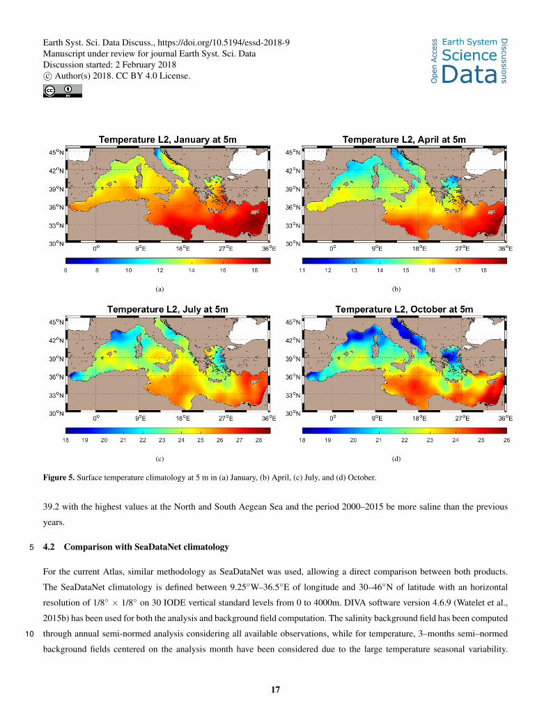
Figure 5 illustrates the surface temperature at 5 m in January, April, July and October and represents the seasonal cycle of
the thermal field with a mean shift of 9◦C between January and July. The Western Mediterranean exhibits smaller temperatures
than the Eastern basin. The differences between the northern and southern regions (meridional gradient) are also very well
represented. The Rhodes Gyre, identified by minimum temperature values is distinguished southeast of Crete island, mainly at20
spring and autumn periods.
Some representative seasonal distributions of salinity at 5 m are shown at Fig. 6. The signal of the fresh Atlantic water (AW)
(S ≈ 36.5) and its flow along the Algerian coast towards the eastern basin through the Sicily Strait is very evident. We can also
notice the areas of low salinity due to river runoffs such as the North Adriatic and the North Aegean Sea that is influenced by
the Dardanelles outflow.25
15
Earth Syst. Sci. Data Discuss., https://doi.org/10.5194/essd-2018-9
Ope
n A
cces
s Earth System
Science
DataD
iscussio
ns
Manuscript under review for journal Earth Syst. Sci. DataDiscussion started: 2 February 2018c© Author(s) 2018. CC BY 4.0 License.

(a) (b)
(c) (d)
Figure 4. Example of observations distribution (a) and corresponding fields distributions depending on relative error threshold values, (b)
unmasked field, (c) masked field with relative error threshold=0.3, (d) masked field with relative error threshold=0.5.
Winter salinity fields at 100 m and 500 m respectively are shown at Figs. 7 and 8 for the last four periods (1970–1979,
1980–1989, 1990–1999, and 2000–2015). There is a homogeneous increasing trend from west to east compared to the surface.
The salinity range is between about 37 and 38.6 at 100 m at the western Mediterranean while the periods 1980–1989 and 2000–
2015 are characterized by higher salinities compared to the other periods. Maximum values are found at the south Adriatic at
38.9 the period 1980–1989 and 38.8 the period 2000–2015. At the Eastern Mediterranean, the salinity is between about 38.430
and 39.4 at 100 m with the maxima found in the Levantine basin and Aegean Sea. The last period 2000–2015 is at an average
more saline than the previous ones and the thermohaline circulation patterns (such as the Shikmona Gyre) are more intense.
In the western basin it is characteristic the increase of salinity at 500m compared to the 100m, where it is between about
38.4 and 38.7. This increase is due to the mixing with LIW that flows towards the Strait of Gibraltar. The Tyrrhenian Sea has
higher salinities in the periods 1970–1979 and 2000–2015. In the Eastern Mediterranean the salinity is between about 38.4 and
16
Earth Syst. Sci. Data Discuss., https://doi.org/10.5194/essd-2018-9
Ope
n A
cces
s Earth System
Science
DataD
iscussio
ns
Manuscript under review for journal Earth Syst. Sci. DataDiscussion started: 2 February 2018c© Author(s) 2018. CC BY 4.0 License.
(a) (b)
(c) (d)
Figure 5. Surface temperature climatology at 5 m in (a) January, (b) April, (c) July, and (d) October.
39.2 with the highest values at the North and South Aegean Sea and the period 2000–2015 be more saline than the previous
years.
4.2 Comparison with SeaDataNet climatology5
For the current Atlas, similar methodology as SeaDataNet was used, allowing a direct comparison between both products.
The SeaDataNet climatology is defined between 9.25◦W–36.5◦E of longitude and 30–46◦N of latitude with an horizontal
resolution of 1/8◦ × 1/8◦ on 30 IODE vertical standard levels from 0 to 4000m. DIVA software version 4.6.9 (Watelet et al.,
2015b) has been used for both the analysis and background field computation. The salinity background field has been computed
through annual semi-normed analysis considering all available observations, while for temperature, 3–months semi–normed10
background fields centered on the analysis month have been considered due to the large temperature seasonal variability.
17
Earth Syst. Sci. Data Discuss., https://doi.org/10.5194/essd-2018-9
Ope
n A
cces
s Earth System
Science
DataD
iscussio
ns
Manuscript under review for journal Earth Syst. Sci. DataDiscussion started: 2 February 2018c© Author(s) 2018. CC BY 4.0 License.

(a) (b)
(c) (d)
Figure 6. Surface salinity climatology at 5 m for (a) Winter, (b) Spring, (c) Summer and (d) Autumn.
Figure 9 shows temperature distributions for Atlas and SeaDataNet climatology, for January at 10 m and November at 1000 m.
There is very good consistency between both products. The same good agreement exists among other months and depths (not
shown here). In surface distributions (at 10 m), the data weighting applied in the Atlas (Fig. 9(a)) has reduced the extension of
the influence of Po river.5
Statistical indexes like bias (differences between the two climatologies) and RMSE (Root-Mean-Square Error) show very
good agreement too. Figure 10 shows the basin vertical averages of bias and RMSE between Atlas and SeaDataNet monthly
temperature (a) and monthly salinity (b) climatologies. Higher differences occur in spring and autumn, Atlas is 0.03◦C more
warm than SeaDataNet in June and less warm at 0.02◦C in November. Temperature RMSE values are ranging between 0.09
in February and 0.19 in July. Maximum differences between the two climatologies are located in the first layers (not shown
here) for all months. Atlas has slightly higher than SeaDataNet salinity values at August and December and the mean bias
18
Earth Syst. Sci. Data Discuss., https://doi.org/10.5194/essd-2018-9
Ope
n A
cces
s Earth System
Science
DataD
iscussio
ns
Manuscript under review for journal Earth Syst. Sci. DataDiscussion started: 2 February 2018c© Author(s) 2018. CC BY 4.0 License.

(a) (b)
(c) (d)
Figure 7. Winter salinity at 100 m for four periods: (a) 1970–1979, (b) 1980–1989, (c) 1990–1999, (d) 2000–2015.
value throughout the year is 0.003. Salinity RMSE values are ranging between 0.048 and 0.076. As for temperature, maximum
differences are located in the first layers for al months.
4.3 Comparison with World Ocean Atlas (WOA13)5
WOA13 provides objectively analyzed annual, seasonal and monthly fields covering the time period 1955–2012 (average of
six decadal means), and six decades: 1955–1964, 1965–1974, 1975–1984, 1985–1994, 1995–2004, 2005–2012. Each decadal
climatology consists of annual (computed as 12-months averages); seasonal: Winter (Jan–Mar), Spring (Apr–Jun), Summer
(Jul–Sep), Fall (Oct–Dec) computed as 3-month averages; and monthly fields (above 1500 m). Annual, seasonal and monthly
temperature and salinity fields are available on 1◦ × 1◦ and 1/4◦ × 1/4◦ latitude/longitude grids. All annual and seasonal fields10
were calculated from 0 to 5500 m depth on 102 standard levels. Monthly fields are available only above 1500 m on all grids
19
Earth Syst. Sci. Data Discuss., https://doi.org/10.5194/essd-2018-9
Ope
n A
cces
s Earth System
Science
DataD
iscussio
ns
Manuscript under review for journal Earth Syst. Sci. DataDiscussion started: 2 February 2018c© Author(s) 2018. CC BY 4.0 License.

(a) (b)
(c) (d)
Figure 8. Winter salinity at 500 m for four periods: (a) 1970–1979, (b) 1980–1989, (c) 1990–1999, (d) 2000–2015.
on 57 standard levels. Figure 11 shows temperature fields for Atlas and WOA13 for January at 0 m and September 1000 m. At
the surface, the Atlas is able to represent the January mean state with more details.
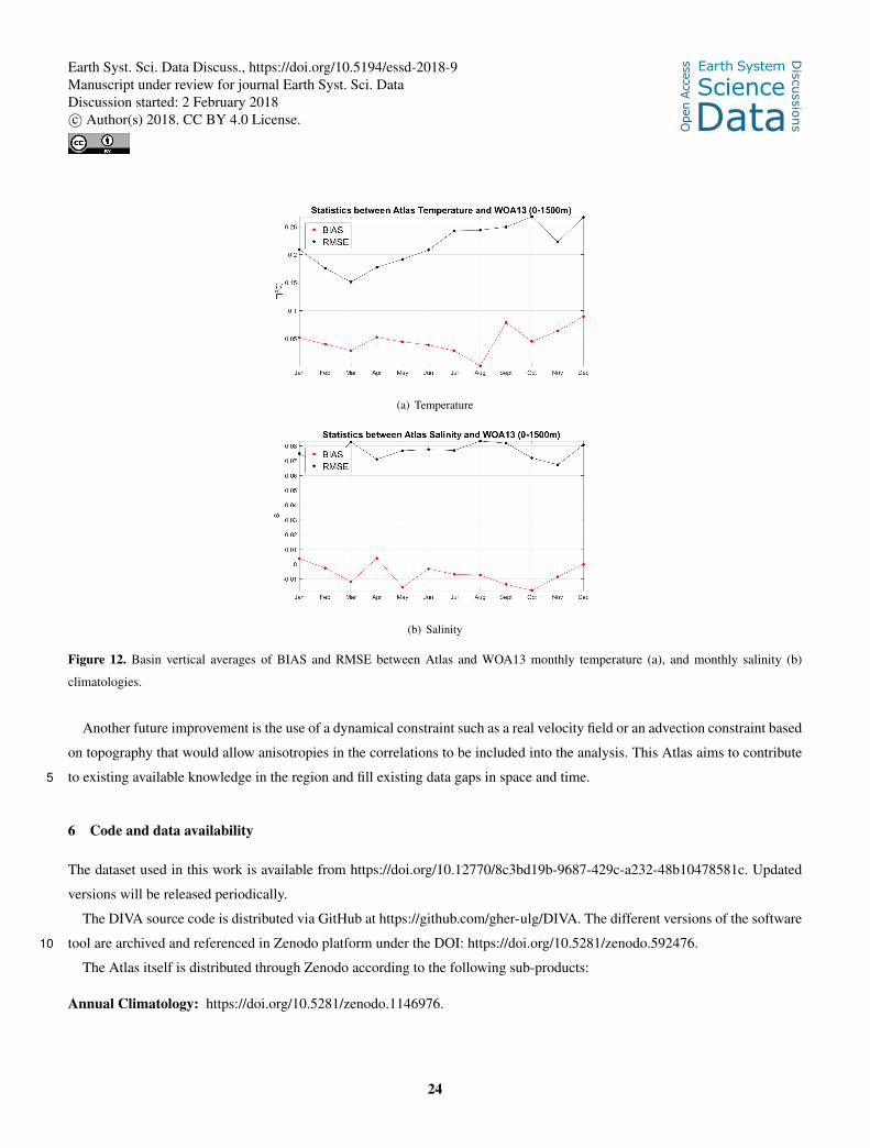
Statistical indexes to quantify the differences between several vertical averages have been calculated also which show a
very good agreement between both monthly T/S climatologies. Figure 12 shows the basin vertical averages of bias and RMSE5
between Atlas and WOA13 monthly temperature (a) and monthly salinity (b) climatologies. Temperature bias is always positive
indicating that the Atlas is slightly warmer than the WOA13 climatology. Atlas salinity is less than the WOA13 at an average
of 0.007 throughout the whole year.
20
Earth Syst. Sci. Data Discuss., https://doi.org/10.5194/essd-2018-9
Ope
n A
cces
s Earth System
Science
DataD
iscussio
ns
Manuscript under review for journal Earth Syst. Sci. DataDiscussion started: 2 February 2018c© Author(s) 2018. CC BY 4.0 License.

(a) (b)
(c) (d)
Figure 9. Comparison of Atlas temperature (left) and SeaDataNet climatology (right) between January at 10 m (top) and November at
1000 m (bottom).
4.4 Comparison with Medar/Medatlas Climatology
The Medar/Medatlas climatology was computed using the Variational Inverse Method (VIM) as the current Atlas. Correlation
length was fixed a priori to a constant value according to the a priori knowledge of typical scales of parameters in the domain
of interest. The signal-to-noise ratio was calibrated by a Generalized Cross Validation technique. Data closer than 15 km from
the coast or in areas shallower than 50 m were rejected in order to avoid the influence of coastal features on open sea (Rixen5
et al., 2005).
The impact of such as rejection can be seen in the Fig. 13: in the North Adriatic Sea and in the North Aegean Sea, the
influence of Po river and Black Sea outflows during winter are not captured.
21
Earth Syst. Sci. Data Discuss., https://doi.org/10.5194/essd-2018-9
Ope
n A
cces
s Earth System
Science
DataD
iscussio
ns
Manuscript under review for journal Earth Syst. Sci. DataDiscussion started: 2 February 2018c© Author(s) 2018. CC BY 4.0 License.

(a) Temperature
(b) Salinity
Figure 10. Basin vertical averages of BIAS and RMSE between Atlas and SeaDataNet monthly temperature (a), and monthly salinity (b)
climatologies.
The temperature at 10 m for the decade 1991–2000 is shown below for the Atlas (Fig. 14(a)) and the Medar/Medatlas
climatology (Fig. 14(b)). The Medar/Medatlas profiles extend until 2000, so this decade was chosen as the most complete one
since there is no error field available to mask regions empty of data.
As it can be seen in Fig. 14, the current Atlas describes with more detail the several features of the general circulation pattern.
5 Conclusions5
A new, high-resolution Atlas of temperature and salinity for the Mediterranean Sea for the period 1950–2015 is presented. The
analysis is based on the latest SeaDataNet dataset, providing the most complete, extended and improved collection of in-situ
observations.
The results describe well the expected distributions of the hydrological characteristics and reveal their long term changes.
Techniques for overcoming the inhomogeneous vertical and spatial distribution of oceanographic measurements were pre-10
sented. The analysis focused on data of 1950 and onwards where more reliable instrumental observations exist. Comparisons
with SeaDataNet reveal a very good agreement. It was expected since both two climatologies use similar interpolation method-
22
Earth Syst. Sci. Data Discuss., https://doi.org/10.5194/essd-2018-9
Ope
n A
cces
s Earth System
Science
DataD
iscussio
ns
Manuscript under review for journal Earth Syst. Sci. DataDiscussion started: 2 February 2018c© Author(s) 2018. CC BY 4.0 License.

(a) (b)
(c) (d)
Figure 11. Comparison of Atlas temperature (left) and WOA13 climatology (right) between January at 0 m (top) and September at 1000 m
(bottom).
ology. The Atlas offers additional value-added decadal temperature and salinity distributions which already exist in the region
from previous versions of Medar/Medatlas climatology though with no error fields available. This is of particular importance.
There are still improvements to be implemented in future versions of the atlas, such as a three-dimensional analysis instead of
stacking the two-dimensional horizontal levels together in order to take into account the vertical correlation of the parameters.
This would reduce vertical inconsistencies that may remain in the results. In addition, the correction of the warm bias in the5
bathythermographs data, caused by instrumental errors, should also be addressed. However it is anticipated that the approach
followed here concerning the calibration of the analysis parameters will be followed by other groups in the future for the
Mediterranean climate studies and other applications related with the long term variability of the hydrological characteristics
of the region and its climate change.
23
Earth Syst. Sci. Data Discuss., https://doi.org/10.5194/essd-2018-9
Ope
n A
cces
s Earth System
Science
DataD
iscussio
ns
Manuscript under review for journal Earth Syst. Sci. DataDiscussion started: 2 February 2018c© Author(s) 2018. CC BY 4.0 License.
(a) Temperature
(b) Salinity
Figure 12. Basin vertical averages of BIAS and RMSE between Atlas and WOA13 monthly temperature (a), and monthly salinity (b)
climatologies.
Another future improvement is the use of a dynamical constraint such as a real velocity field or an advection constraint based
on topography that would allow anisotropies in the correlations to be included into the analysis. This Atlas aims to contribute
to existing available knowledge in the region and fill existing data gaps in space and time.5
6 Code and data availability
The dataset used in this work is available from https://doi.org/10.12770/8c3bd19b-9687-429c-a232-48b10478581c. Updated
versions will be released periodically.
The DIVA source code is distributed via GitHub at https://github.com/gher-ulg/DIVA. The different versions of the software
tool are archived and referenced in Zenodo platform under the DOI: https://doi.org/10.5281/zenodo.592476.10
The Atlas itself is distributed through Zenodo according to the following sub-products:
Annual Climatology: https://doi.org/10.5281/zenodo.1146976.
24
Earth Syst. Sci. Data Discuss., https://doi.org/10.5194/essd-2018-9
Ope
n A
cces
s Earth System
Science
DataD
iscussio
ns
Manuscript under review for journal Earth Syst. Sci. DataDiscussion started: 2 February 2018c© Author(s) 2018. CC BY 4.0 License.

(a) (b)
(c) (d)
Figure 13. January temperature at 10 m: (a) Medar/Medatlas, coastal data removed from the analysis; (b) data used; (c) current climatology,
coastal data included; (d) data used.
Seasonal Climatology for 57 running decades from 1950-1959 to 2006-2015:
https://doi.org/10.5281/zenodo.1146938.
Seasonal Climatology: https://doi.org/10.5281/zenodo.1146953.5
Annual Climatology for 57 running decades from 1950-1959 to 2006-2015:
https://doi.org/10.5281/zenodo.1146957.
Seasonal Climatology for six periods: 1950-1959, 1960-1969, 1970-1979, 1980-1989, 1990-1999, 2000-2015:
https://doi.org/10.5281/zenodo.1146966.
25
Earth Syst. Sci. Data Discuss., https://doi.org/10.5194/essd-2018-9
Ope
n A
cces
s Earth System
Science
DataD
iscussio
ns
Manuscript under review for journal Earth Syst. Sci. DataDiscussion started: 2 February 2018c© Author(s) 2018. CC BY 4.0 License.

(a) (b)
Figure 14. (a) Atlas masked temperature field for the decade 1991–2000 at 10 m, (b) Medar/Medatlas temperature field for the decade
1991–2000, at 10 m (no error field is available).
Annual Climatology for six periods: 1950-1959, 1960-1969, 1970-1979, 1980-1989, 1990-1999, 2000-2015:
https://doi.org/10.5281/zenodo.1146970.
Monthly Climatology: https://doi.org/10.5281/zenodo.1146974.
Author contributions. A.I. created the Atlas, wrote the first version of the manuscript and prepared the figures. JMB, S.W., C.T. and A.T.
reviewed the manuscript. C.T. and S.W. formatted the document in LaTeX.5
Competing interests. The authors declare no competing interests.
Disclaimer. It cannot be warranted that the Atlas is free from errors or omissions. Correct and appropriate Atlas interpretation and usage is
solely the responsibility of data users.
Acknowledgements. The DIVA development has received funding from the European Union Sixth Framework Programme (FP6/2002–2006)
under grant agreement no. 026212, SeaDataNet, Seventh Framework Programme (FP7/2007–2013) under grant agreement no. 283607,10
SeaDataNet II, SeaDataCloud and EMODnet (MARE/2008/03 - Lot 3 Chemistry - SI2.531432) from the Directorate-General for Maritime
Affairs and Fisheries.
26
Earth Syst. Sci. Data Discuss., https://doi.org/10.5194/essd-2018-9
Ope
n A
cces
s Earth System
Science
DataD
iscussio
ns
Manuscript under review for journal Earth Syst. Sci. DataDiscussion started: 2 February 2018c© Author(s) 2018. CC BY 4.0 License.

References
Beckers, J.-M., Barth, A., Troupin, C., and Alvera-Azcárate, A.: Some approximate and efficient methods to assess error fields in spa-
tial gridding with DIVA (Data Interpolating Variational Analysis), Journal of Atmospheric and Oceanic Technology, 31, 515–530,15
https://doi.org/10.1175/JTECH-D-13-00130.1, http://journals.ametsoc.org/doi/abs/10.1175/JTECH-D-13-00130.1, 2014.
Bergamasco, A. and Malanotte-Rizzoli, P.: The circulation of the Mediterranean Sea: a historical review of experimental investigations,
Advances in Oceanography and Limnology, 1, 11–28, https://doi.org/10.1080/19475721.2010.491656, http://www.tandfonline.com/doi/
abs/10.1080/19475721.2010.491656, 2010.
Béthoux, J.-P., Gentili, B., and Tailliez, D.: Warming and freshwater budget change in the Mediterranean since the 1940s, their possible20
relation to the greenhouse effect, Geophysical Research Letters, 25, 1023–1026, https://doi.org/10.1029/98gl00724, http://onlinelibrary.
wiley.com/doi/10.1029/98GL00724/abstract, 1998.
Brankart, J.-M. and Brasseur, P.: Optimal analysis of In Situ Data in the Western Mediterranean Using Statistics and Cross-Validation.,
Journal of Atmospheric and Oceanic Technology, 13, 477–491, https://doi.org/10.1175/1520-0426(1996)013<0477:OAOISD>2.0.CO;2,
1996.25
Brankart, J.-M. and Brasseur, P.: The general circulation in the Mediterranean Sea: a climatological approach., Journal of Marine Systems,
18, 41–70, https://doi.org/10.1016/S0924-7963(98)00005-0, 1998.
Brasseur, P., Beckers, J., Brankart, J., and Schoenauen, R.: Seasonal temperature and salinity fields in the Mediterranean Sea: Climatological
analyses of a historical data set, Deep Sea Research Part I: Oceanographic Research Papers, 43, 159–192, https://doi.org/10.1016/0967-
0637(96)00012-x, http://dx.doi.org/10.1016/0967-0637(96)00012-X, 1996.30
Bretherton, F., Davis, R., and Fandry, C.: A technique for objective analysis and design of oceanic experiments applied to Mode-73, Deep-Sea
Research, 23, 559–582, https://doi.org/10.1016/0011-7471(76)90001-2, 1976.
Capet, A., Troupin, C., Carstensen, J., Grégoire, M., and Beckers, J.-M.: Untangling spatial and temporal trends in the variability of the
Black Sea Cold Intermediate Layer and mixed Layer Depth using the DIVA detrending procedure, Ocean Dynamics, 64, 315–324,
https://doi.org/10.1007/s10236-013-0683-4, http://link.springer.com/article/10.1007%2Fs10236-013-0683-4, 2014.35
Gandin, L. S.: Objective analysis of meteorological fields. By L. S. Gandin. Translated from the Russian. Jerusalem (Israel Program for Sci-
entific Translations), 1965, Quarterly Journal of the Royal Meteorological Society, 92, 447–447, https://doi.org/10.1002/qj.49709239320,
http://onlinelibrary.wiley.com/doi/10.1002/qj.49709239320/abstract, 1966.
Guibout, P.: Atlas Hydrologique de la Mediterranee, Shom, Ifremer, Paris, France, 1 edn., 150 pp, 1987.
Hecht, A., Pinardi, N., and Robinson, A. R.: Currents, Water Masses, Eddies and Jets in the Mediterranean Levantine Basin, Journal
of Physical Oceanography, 18, 1320–1353, https://doi.org/10.1175/1520-0485(1988)018<1320:CWMEAJ>2.0.CO;2, https://doi.org/10.5
1175/1520-0485(1988)018<1320:CWMEAJ>2.0.CO;2, 1988.
INGV: Mediterranean Sea - Temperature and salinity observation collection V2, Tech. rep., Istituto Nazionale di Geofisica e Vulcanologia,
Sede di Bologna, https://doi.org/10.12770/8c3bd19b-9687-429c-a232-48b10478581c, 2015.
La Violette, P. E.: The Western Mediterranean Circulation Experiment (WMCE): Introduction, Journal of Geophysical Research, 95, 1511,
https://doi.org/10.1029/jc095ic02p01511, http://dx.doi.org/10.1029/JC095iC02p01511, 1990.10
Levitus, S.: Climatological Atlas of the World Ocean, Tech. rep., NOAA Professional Paper 13. US. Government Printing Office: Washington,
DC, 1982.
27
Earth Syst. Sci. Data Discuss., https://doi.org/10.5194/essd-2018-9
Ope
n A
cces
s Earth System
Science
DataD
iscussio
ns
Manuscript under review for journal Earth Syst. Sci. DataDiscussion started: 2 February 2018c© Author(s) 2018. CC BY 4.0 License.

Locarnini, R. A., Mishonov, A. V., Antonov, J. I., Boyer, T. P., Garcia, H. E., Baranova, O. K., Zweng, M. M., Paver, C. R., Reagan, J. R.,
Johnson, D. R., Hamilton, M., and Seido, D.: World Ocean Atlas 2013, Volume 1: Temperature, in: NOAA Atlas NESDIS, edited by
S. Levitus, Ed., A. M. T. E., vol. 73, p. 40 pp, NOAA, http://data.nodc.noaa.gov/woa/WOA13/DOC/woa13_vol1.pdf, 2013.15
Lozier, M. S., Owens, W. B., and Curry, R. G.: The climatology of the North Atlantic, Progress in Oceanography, 36, 1–
44, https://doi.org/10.1016/0079-6611(95)00013-5, http://www.sciencedirect.com/science/article/pii/0079661195000135?via%3Dihub,
1995.
Malanotte-Rizzoli, P. and Hecht, A.: Large-scale properties of the eastern mediterranean: a rewiew, Oceanologica Acta, 11, 323–335, 1988.
Manca, B., Burca, M., Giorgetti, A., Coatanoan, C., Garcia, M.-J., and Iona, A.: Physical and biochemical averaged vertical profiles20
in the Mediterranean regions: an important tool to trace the climatology of water masses and to validate incoming data from op-
erational oceanography, Journal of Marine Systems, 48, 83 – 116, https://doi.org/https://doi.org/10.1016/j.jmarsys.2003.11.025, http:
//www.sciencedirect.com/science/article/pii/S0924796304000090, tracer Methods in Geophysical Fluid Dynamics, 2004.
MEDAR Group: MEDATLAS/2002 database. Mediterranean and Black Sea database of temperature salinity and bio-chemical parameters.
Climatological Atlas, Tech. rep., Ifremer, 4 Cdroms, 2002.25
Millot, C.: Circulation in the Western Mediterranean Sea, Oceanologica Acta, 10, 143–148, 1987.
Millot, C.: Mesoscale and seasonal variabilities of the circulation in the western Mediterranean, Dynamics of Atmospheres and
Oceans, 15, 179 – 214, https://doi.org/https://doi.org/10.1016/0377-0265(91)90020-G, http://www.sciencedirect.com/science/article/pii/
037702659190020G, 1991.
Millot, C.: Circulation in the Western Mediterranean Sea, Journal of Marine Systems, 20, 423 – 442,30
https://doi.org/https://doi.org/10.1016/S0924-7963(98)00078-5, http://www.sciencedirect.com/science/article/pii/S0924796398000785,
1999.
Ovchinnikov, I.: Circulation in the surface and intermediate layers of the mediterranean, Oceanology, 6, 49–59, 1966.
Picco, P.: Climatological Atlas of the Western Mediterranean, Tech. rep., ENEA Santa Teresa Centre, La Spezia, Italy, 224 pp, 1990.
Rahmstorf, S.: Influence of mediterranean outflow on climate, Eos, Transactions American Geophysical Union, 79, 281–281,35
https://doi.org/10.1029/98eo00208, http://onlinelibrary.wiley.com/doi/10.1029/98EO00208/abstract, 1998.
Reiniger, R. and Ross, C.: A method of interpolation with application to oceanographic data, Deep-Sea Res., 15, 185–193,
https://doi.org/10.1016/0011-7471(68)90040-5, 1968.
Rixen, M., Beckers, J.-M., Brankart, J.-M., and Brasseur, P.: A numerically efficient data analysis method with error map generation, Ocean
Modelling, 2, 45–60, https://doi.org/10.1016/S1463-5003(00)00009-3, 2000.
Rixen, M., Beckers, J.-M., and Allen, J.: Diagnosis of vertical velocities with the QG Omega equation: a relocation method to obtain
pseudo-synoptic data sets, Deep Sea Research Part I: Oceanographic Research Papers, 48, 1347–1373, https://doi.org/10.1016/S0967-5
0637(00)00085-6, http://www.sciencedirect.com/science/article/pii/S0967063700000856, 2001.
Rixen, M., Beckers, J.-M., Levitus, S., Antonov, J., Boyer, T., Maillard, C., Fichaut, M., Balopoulos, E., Iona, S., Dooley, H., Garcia, M.-J.,
Manca, B., Giorgetti, A., Manzella, G., Mikhailov, N., Pinardi, N., Zavatarelli, M., and the Medar Consortium: The Western Mediterranean
Deep Water: a proxy for global climate change, Geophysical Research Letters, 32, L12 608, https://doi.org/10.1029/2005GL022702,
http://www.agu.org/pubs/crossref/2005/2005GL022702.shtml, 2005.10
Robinson, A., Leslie, W., Theocharis, A., and Lascaratos, A.: Mediterranean Sea Circulation, Encyclopedia of Ocean Sciences, pp. 1689–
1705, https://doi.org/10.1006/rwos.2001.0376, http://www.sciencedirect.com/science/article/pii/B012227430X003767, 2001.
28
Earth Syst. Sci. Data Discuss., https://doi.org/10.5194/essd-2018-9
Ope
n A
cces
s Earth System
Science
DataD
iscussio
ns
Manuscript under review for journal Earth Syst. Sci. DataDiscussion started: 2 February 2018c© Author(s) 2018. CC BY 4.0 License.

Schlitzer, R.: Interactive analysis and visualization of geoscience data with Ocean Data View, Computers & Geosciences,
28, 1211–1218, https://doi.org/10.1016/S0098-3004(02)00040-7, http://www.sciencedirect.com/science/article/B6V7D-46TB0P2-C/2/
49937e4939d29fab010dc7f0af310bc8, 2002.15
SeaDataNet Group: Data Quality Control Procedures, Tech. Rep. Version 2.0, SeaDataNet consortium, https://www.seadatanet.org/content/
download/596/3118/file/SeaDataNet_QC_procedures_V2_%28May_2010%29.pdf?version=1, 2010.
Simoncelli, S., Coatanoan, C., Myroshnychenko, V., Sagen, H., Bäck, O., Scory, S., Grandi, A., Barth, A., and Fichaut, M.: Sea-
DataNet. First Release of Regional Climatologies. WP10 Third Year Report - DELIVERABLE D10.3., Tech. rep., SeaDataNet,
https://doi.org/10.13155/50381, 2015.20
Troupin, C., Machín, F., Ouberdous, M., Sirjacobs, D., Barth, A., and Beckers, J.-M.: High-resolution Climatology of the
North-East Atlantic using Data-Interpolating Variational Analysis (Diva), Journal of Geophysical Research, 115, C08 005,
https://doi.org/10.1029/2009JC005512, http://onlinelibrary.wiley.com/doi/10.1029/2009JC005512/epdf, 2010.
Troupin, C., Sirjacobs, D., Rixen, M., Brasseur, P., Brankart, J.-M., Barth, A., Alvera-Azcárate, A., Capet, A., Ouberdous, M., Lenartz, F.,
Toussaint, M.-E., and Beckers, J.-M.: Generation of analysis and consistent error fields using the Data Interpolating Variational Analysis25
(Diva), Ocean Modelling, 52-53, 90–101, https://doi.org/10.1016/j.ocemod.2012.05.002, http://www.sciencedirect.com/science/article/
pii/S1463500312000790, 2012.
Troupin, C., Watelet, S., Barth, A., and Beckers, J.-M.: Diva-User-Guide: v1.0 (Version v1.0). Zenodo., Tech. rep., GeoHydrodynamics and
Environment Research, University of Liège, Liège, Belgium, https://doi.org/10.5281/zenodo.836723, 2017.
Watelet, S., Ouberdous, M., Troupin, C., Barth, A., and Beckers, J.-M.: DIVA Version 4.6.11, Tech. rep., GeoHydrodynamics and Environ-
ment Research, University of Liège, Liège, Belgium, https://doi.org/10.5281/zenodo.400970, 2015a.535
Watelet, S., Ouberdous, M., Troupin, C., Barth, A., and Beckers, J.-M.: DIVA Version 4.6.9, Tech. rep., GeoHydrodynamics and Environment
Research, University of Liège, Liège, Belgium, https://doi.org/10.5281/zenodo.400968, 2015b.
Watelet, S., Troupin, C., Beckers, J.-M., Barth, A., and Ouberdous, M.: DIVA Version 4.7.1, Tech. rep., GeoHydrodynamics and Environment
Research, University of Liège, Liège, Belgium, https://doi.org/10.5281/zenodo.836727, 2017.
Wijffels, S. E., Willis, J., Domingues, C. M., Barker, P., White, N. J., Gronell, A., Ridgway, K., and Church, J. A.: Changing Expend-540
able Bathythermograph Fall Rates and Their Impact on Estimates of Thermosteric Sea Level Rise, Journal of Climate, 21, 5657–5672,
https://doi.org/10.1175/2008jcli2290.1, http://dx.doi.org/10.1175/2008JCLI2290.1, 2008.
Zweng, M., Reagan, J., Antonov, J., Locarnini, R., Mishonov, A., Boyer, T., Garcia, H., Baranova, O., Johnson, D., D.Seidov, and Biddle,
M.: World Ocean Atlas 2013, Volume 2: Salinity, in: NOAA Atlas NESDIS, edited by S. Levitus, Ed., A. M. T. E., vol. 74, p. 39 pp,
NOAA, http://data.nodc.noaa.gov/woa/WOA13/DOC/woa13_vol2.pdf, 2013.545
29
Earth Syst. Sci. Data Discuss., https://doi.org/10.5194/essd-2018-9
Ope
n A
cces
s Earth System
Science
DataD
iscussio
ns
Manuscript under review for journal Earth Syst. Sci. DataDiscussion started: 2 February 2018c© Author(s) 2018. CC BY 4.0 License.