Embed Size (px)
Citation preview

2014/53 ■
Forecasting comparison of long term component dynamic models for realized covariance matrices
Luc Bauwens, Manuela Braione and Giuseppe Storti
Center for Operations Research and Econometrics
Voie du Roman Pays, 34
B-1348 Louvain-la-Neuve Belgium
http://www.uclouvain.be/core
D I S C U S S I O N P A P E R

CORE Voie du Roman Pays 34, L1.03.01 B-1348 Louvain-la-Neuve, Belgium. Tel (32 10) 47 43 04 Fax (32 10) 47 43 01 E-mail: [email protected] http://www.uclouvain.be/en-44508.html

CORE DISCUSSION PAPER 2014/53
Forecasting comparison of long term component dynamic models for realized covariance matrices
Luc BAUWENS1, Manuela BRAIONE2 and Giuseppe STORTI3
November 2014
Abstract
Novel model specifications that include a time-varying long run component in the dynamics of realized covariance matrices are proposed. The adopted modeling framework allows the secular component to enter the model structure either in an additive fashion or as a multiplicative factor, and to be specified parametrically, using a MIDAS filter, or non-parametrically. Estimation is performed by maximizing a Wishart quasi-likelihood function. The one-step ahead forecasting performance of the models is assessed by means of three approaches: the Model Confidence Set, (global) minimum variance portfolios and Value-at-Risk. The results provide evidence in favour of the hypothesis that the proposed models outperform benchmarks incorporating a constant long run component, both in and out-of-sample. Keywords: Realized covariance, component dynamic models, MIDAS, minimum variance portfolio, Model Confidence Set, Value-at-Risk. JEL Classification: C13, C32, C58.
1 Université catholique de Louvain, CORE, B-1348 Louvain-La-Neuve, Belgium; University of Johannesburg, Department of Economics and Econometrics, Auckland Park 2006, Johannesburg, South Africa. Email: [email protected] 2 Université catholique de Louvain, CORE, B-1348 Louvain-La-Neuve, Belgium. Email: [email protected] 3 Department of Economics and Statistics, Università di Salerno, Fisciano, Italy. E-mail: [email protected] Luc Bauwens and Manuela Braione acknowledge support of the “Communauté française de Belgique" through contract “Projet d'Actions de Recherche Concertées 12/17-045", granted by the “Académie universitaire Louvain". Giuseppe Storti acknowledges funding from the Italian Ministry of Education, University and Research (MIUR) through PRIN project “Forecasting economic and financial time series: understanding the complexity and modeling structural change" (code 2010J3LZEN).

1 Introduction
Volatility models that include a time-varying long run component have been increasingly used
over the last decade. Empirical evidence has indeed suggested that the level of variances and
correlations is changing over time as a function of economic conditions. This can have important
forecasting implications, as models reverting to a constant level in the long run will produce the
same long term forecast at any point in time, thus completely ignoring the changing economic
conditions. Without controlling for the different sources affecting volatility, they will end up
producing spurious forecasts.
Since Engle & Lee (1999) introduced a GARCH model with additive long run and short
run dynamic components, several others have proposed related component models for volatil-
ity. Engle & Rangel (2008) specify a semi-parametric model that allows for time-variation in
the unconditional level of stock market volatility, while Engle et al. (2008) use a parametric
specification involving the Mixed Data Sampling (MIDAS) scheme to extract a slowly moving
secular component around which daily volatility moves. Specifically, the short run component
is a GARCH specification based on daily squared returns, while the long run component is
driven by realized volatilities computed over a monthly, quarterly or biannual basis. The idea
has been extended to dynamic correlations in the DCC-MIDAS of Colacito et al. (2011) and in
the multiplicative-DCC of Bauwens et al. (2013).
More recently, researchers have paid attention to the specification of models directly fitted
to time series of realized covariances. As advocated by Andersen et al. (2003), high-frequency
based models produce significant improvements in predictive performance relative to models
that rely on daily data alone. Pioneering works in this respect can be found in Gourieroux et al.
(2009), Jin & Maheu (2013), and Chiriac & Voev (2011), among others. Our approach is closer
to Golosnoy et al. (2012), who proposed a model where the realized covariance matrix of asset
returns is assumed to follow a conditional Wishart distribution with a time-varying conditional
expectation that is inspired by the BEKK model of the multivariate GARCH literature. This
conditionally autoregressive Wishart (CAW) model aims to capture the daily dynamics of the
realized covariances around a constant level matrix. Golosnoy et al. (2012) also propose an
extension of their basic model specifically designed to capture long run fluctuations in the
levels of covariances, by replacing the constant level matrix by a MIDAS filter of past realized
covariance matrices. They apply their models to daily realized covariance matrices for the
returns of five stocks and show that the MIDAS-CAW specification dominates the baseline
CAW model both in-sample and out-of-sample. That application involves estimating more
than one hundred parameters due to the use of a full BEKK specification and thus it is difficult
1

to apply this model in a higher dimensional setting.
Inspired by this approach, we propose a wider set of models for realized covariance matrices
which account both for time variation in the long run levels of (co)volatilities and for their
short-run dynamics around these levels, and are applicable in higher dimensions.
Similarly to Golosnoy et al. (2012), we decompose the conditional expectation of the realized
covariance matrix into a slowly evolving process and a mean-reverting short run one. We extend
the existing framework discussed so far mainly into two directions. First, our modeling setting
allows the long-run component to enter the model structure either in additive fashion, as a time-
varying intercept in the volatility and correlation (or covariance) models, or as a multiplicative
factor. This allows us to specify it parametrically, using a MIDAS-type filter, or even non-
parametrically, by means of a matrix-variate smoother. Second, we exploit the advantages of a
parsimonious modeling of the short run dynamics by employing different specifications inspired
by the multivariate GARCH literature, namely scalar BEKK, DCC and DECO-type models.
The estimation of the models is performed by maximizing in one step the likelihood function
based on the conditional Wishart assumption. As shown in Bauwens et al. (2012) and Noureldin
et al. (2012), the function has a quasi-likelihood interpretation and the estimator is consistent
even if the assumed underlying distribution is not Wishart.
The remainder of the paper is organized as follows. In Section 2 we introduce the set of time-
varying long term component models and we explain in detail the different component structures
employed. The procedure for quasi-maximum likelihood (QML) estimation of the proposed
models is covered in Section 3. Section 4 presents the results of an empirical application to a
set of ten U.S. stocks. Specifically, we first compare the in-sample goodness of fit of the different
models in terms of standard information criteria, then we evaluate their forecasting performance
by means of three approaches: the Model Confidence Set, (global) minimum variance portfolios
and Value-at-Risk. Overall, our results illustrate the potential benefits deriving from using
models that include a time-varying long run component against models incorporating a constant
long run component. Section 5 concludes the paper with some final remarks.
2 Component models for realized covariance matrices
The purpose of this section is to formally present the new multivariate time-varying long term
component dynamic models for realized volatilities and correlations of asset returns. Within
each subsection, models incorporating a constant long run component are derived as special
cases. They will be used as benchmarks in the empirical analysis. As a first step, in the next
2

subsection, we define the common modeling framework and provide some preliminary notations.
2.1 General framework
Let Ct be a positive definite and symmetric (PDS) daily realized covariance matrix of order n.
We assume that conditionally on past information It−1 consisting of Cτ for τ ≤ t−1, Ct follows
a n-dimensional central Wishart distribution:
Ct|It−1 ∼ Wn(ν, St/ν), ∀t = 1, . . . , T (1)
where ν (> n− 1) is the degrees of freedom parameter and St/ν is a PDS scale matrix of order
n. From the properties of the Wishart distribution – see e.g. Anderson (1984) – it follows that
the conditional mean is
E(Ct|It−1) = St, (2)
so that the matrix St is referred to as the conditional covariance matrix of rt in the sequel, and
any of its off-diagonal element as a conditional covariance (or variance for a diagonal element).
Equations (1)-(2) define a generic conditional autoregressive Wishart (CAW) model as pro-
posed by Golosnoy et al. (2012). A CAW model specifies the dynamic dependence of the {Ct}
process through a dynamic equation for the scale matrix St of the Wishart distribution, so as to
capture the serial dependences in the realized variances and covariances. In addition, St can be
further designed to directly capture the long run fluctuations in the levels around which realized
variances and covariances or correlations fluctuate from day to day. To this extent, the realized
covariance dynamics are split in two components, a secular smoothly varying component and
a short lived one. In the next subsections, we define several ways to specify both components.
2.2 Long term additive component models for correlations
The structure of the first set of models is inspired by the DCC-MIDAS model of Colacito et al.
(2011). In that model, conditional variances and correlations are modelled separately. We
retain the original model structure but we adapt it to the realized covariance framework. More
specifically, the scale matrix St in Eq.(2) is decomposed in terms of standard deviations and
correlations:
St = DtRtDt, (3)
where the i-th entry of the diagonal matrix Dt = {diag(St)}1/2 is given by the conditional
standard deviation√Sii,t of asset i, and Rt is the corresponding conditional correlation matrix
3

of rt. Notice that the terms ’conditional’ are used for convenience and do not imply that√Sii,t is the conditional mean of
√Cii,t, and that Rt is the conditional mean of the correlation
matrix obtained from Ct. This structure allows us to model separately conditional variances
and correlations, in the spirit of Engle (2002) and Tse & Tsui (2002). Moreover, by ruling out
spillover effects between conditional variances, each univariate volatility model can be specified
and estimated independently of the others.
Baseline models Short and long term dynamic components are accounted for, but separately
treated. Namely, for every t, each conditional volatility is expressed as the product of two
components:
E(Cii,t|It−1) = Sii,tSii,t,
with Sii,t and Sii,t denoting the secular and the mean-reverting short run component, respec-
tively. For each asset i = 1, ..., n, the short run component is specified as a mean reverting
GARCH(1,1)-type process:
Sii,t = (1− γi − δi) + γiCii,t−1
Sii,t−1
+ δiSii,t−1, (4)
where mean-reversion to unity is imposed for identification and stationarity is assured by im-
posing the usual restriction γi + δi < 1.
The secular component is specified using a MIDAS filter assumed to be a weighted sum of
a judiciously chosen number L of lagged realized variances:
Sii,t = mi + θi
L∑l=1
φl(ωs)Cii,t−l, l = 1, ..., L, (5)
where mi and θi are restricted to be positive scalars. Differently from Colacito et al. (2011),
who specify Sii,t as a locally constant long run component, we define it based on rolling samples
that change from day to day. The weight function φl(ωs), normalized so that the sum of the
weights is equal to one, is specified according to the Beta function, defined as
φl(ωs) =
(lL
)ω1s−1 (1− l
L
)ω2s−1∑Lj=1
(jL
)ω1s−1 (1− j
L
)ω2s−1 , (6)
where for brevity, φ(ωs) = φ(ω1s, ω2s). We use the subscript s to differentiate ωs from the
similar scheme that is introduced below for correlations. In order to ensure a decaying pattern
of the weights, it suffices to impose ω1s = 1 and estimate ω2s under the restriction ω2s > 1;
after this, the decaying speed of the weights over time is determined by the data. It should
be obvious that the number of lags L can be chosen high enough so as to obtain a sufficiently
smooth path of the long run component. In order to avoid truncating at too low a lag, which
4

could hide important long run dependences, we set L equal to 264 so as to cover a period of
one year.
The component structure for the conditional correlation matrix is inspired by the same
ideas. The main element is to replace the constant intercept matrix in the DCC specification
by a time-varying component expressed as a weighted average of past realized correlations.
This amounts to specify Rt as
RDCCt = (1− α− β)Pt + αPt−1 + βRDCC
t−1 , (7)
Pt =L∑l=1
φl(ωr)Pt−l, (8)
where Pt = diag{Ct}−1/2Ctdiag{Ct}−1/2 and φl(ωr) is again a Beta weight function that applies
the same weighting scheme to all the elements of the matrix Pt.
Instead of using the DCC-type specification, the dynamic equicorrelation (DECO) type of
model of Engle & Kelly (2012) can also be used. It is written as
RDECOt = (1− ρt)In + ρtJn, (9)
ρt =1
n(n− 1)
(ι′RDCC
t ι),
where ρt is the equicorrelation parameter at time t and ι denotes a vector of ones.
Equations (4) to (8) denote the Additive Midas Realized DCC (AMReDCC) model, while
replacing Eq. (8) with Eq. (9) gives the AMReDECO model. Note that by imposing θi = 0 in
every univariate volatility equation and assuming a constant long run level for correlations (i.e.
Pt = P ∀t), one obtains the RDCC model of Bauwens et al. (2012) as a particular case. The
RDCC can thus be considered as a benchmark for this class of models, even though it is not
formally nested in the AMReDCC since the latter does not include a constant intercept matrix
in Eq.(7).
Variations of the baseline models Two variations of the baseline models are proposed
below. To start with the conditional volatility dynamics, we propose an alternative specification
for the MIDAS polynomial in Eq.(5), in the spirit of Golosnoy et al. (2012). Specifically, we
aggregate the univariate series of realized variances over a horizon of m trading days and
consider K lagged observations, such that Eq.(5) is rewritten as follows:
Sii,t = mi + θi
K∑k=1
φk(ωs)C(m)ii,t,k (10)
C(m)ii,t,k =
t−m(k−1)−1∑τ=t−mk
Cii,τ , k = 1, ..., K.
5

Clearly, for Equations (5) and (10) to be comparable, one must impose K sufficiently smaller
than L. Namely, by considering a span length of the aggregation period m equal to 22 days
and a number of lags K equal to 12, the series of daily realized variances are aggregated over
a period of one year, thus covering the same time span as in Eq.(5).
A similar variation is applied to the MIDAS component driving the long run correlation
dynamics. The matrix Pt in Eq.(8) is replaced by a weighted sum of past realized correlation
matrices aggregated over the past year, i.e.
Pt =K∑k=1
φk(ωr)P(m)t,k (11)
P(m)t,k =
t−m(k−1)−1∑τ=t−mk
Pτ .
This definition of the time-varying intercept matrix Pt does not yield a correlation matrix and
consequently, RDCCt needs to be rescaled into a conditional correlation matrix. Using Equations
(7)-(8), one just needs to compute
RDCC∗t = diag{RDCC
t }−1/2RDCCt diag{RDCC
t }−1/2. (12)
This new model is defined as Additive Midas Aggregated Realized DCC (AMAReDCC), or
AMAReDECO if the DECO version is used.
The second variation proposed for the specification of the conditional correlation matrix
stems from the fact that the construction of RDCCt in Eq.(7) builds upon daily realized covari-
ances filtered from realized standard deviations rather than conditional standard deviations.
By purging the realized covariance matrices from the conditional standard deviations, one can
eliminate potential heteroskedasticity left in Ct and obtain a potentially cleaner estimator.
Namely, Ct can be transformed to
Cpt = D−1
t CtD−1t , t = 1, ..., T, (13)
and then used to compute the time-varying intercept matrix Pt in Eq. (7). This resembles
the approach used in the two-step estimation of the DCC model of Engle (2002), where the
outer product of the first-stage (estimated) standardized residuals ξt is used to compute the
second-stage conditional correlation matrix Rt = Et−1[ξtξ′t].
By combining the different equations proposed for the conditional variances and correla-
tions with the two structures of the MIDAS filter, we obtain eight additive models that are
summarized in Table 1.
6
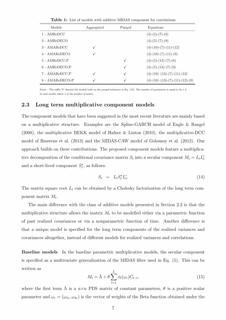
Table 1: List of models with additive MIDAS component for correlations
Models Aggregated Purged Equations
1 - AMReDCC (4)-(5)-(7)-(8)
2 - AMReDECO (4)-(5)-(7)-(9)
3 - AMAReDCC X (4)-(10)-(7)-(11)-(12)
4 - AMAReDECO X (4)-(10)-(7)-(11)-(9)
5 - AMReDCC-P X (4)-(5)-(13)-(7)-(8)
6 - AMReDECO-P X (4)-(5)-(13)-(7)-(9)
7 - AMAReDCC-P X X (4)-(10)–(13)-(7)-(11)-(12)
8 - AMAReDECO-P X X (4)-(10)–(13)-(7)-(11)-(12)-(9)
Notes – The suffix ’P’ denotes the models built on the purged estimator in Eq. (13). The number of parameters is equal to 5n+ 3
in each model, where n is the number of assets.
2.3 Long term multiplicative component models
The component models that have been suggested in the most recent literature are mainly based
on a multiplicative structure. Examples are the Spline-GARCH model of Engle & Rangel
(2008), the multiplicative BEKK model of Hafner & Linton (2010), the multiplicative-DCC
model of Bauwens et al. (2013) and the MIDAS-CAW model of Golosnoy et al. (2012). Our
approach builds on these contributions. The proposed component models feature a multiplica-
tive decomposition of the conditional covariance matrix St into a secular component Mt = LtL′t
and a short-lived component S?t , as follows:
St = LtS?tL′t. (14)
The matrix square root Lt can be obtained by a Cholesky factorization of the long term com-
ponent matrix Mt.
The main difference with the class of additive models presented in Section 2.2 is that the
multiplicative structure allows the matrix Mt to be modelled either via a parametric function
of past realized covariances or via a nonparametric function of time. Another difference is
that a unique model is specified for the long term components of the realized variances and
covariances altogether, instead of different models for realized variances and correlations.
Baseline models In the baseline parametric multiplicative models, the secular component
is specified as a multivariate generalization of the MIDAS filter used in Eq. (5). This can be
written as
Mt = Λ + θ
L∑l=1
φl(ωr)Ct−l, (15)
where the first term Λ is a n×n PDS matrix of constant parameters, θ is a positive scalar
parameter and ωr = (ω1r, ω2r) is the vector of weights of the Beta function obtained under the
7

restrictions ω1r = 1 and ω2r > 1. This long term component has n(n+ 1)/2 + 2 parameters. It
is worth to emphasize that in sufficiently low dimensions this does not represent an issue, but
the proliferation of parameters in large dimensions will eventually render impossible numerical
maximization of the log-likelihood function. Note that by imposing θ = 0 in the MIDAS
specification of Eq. (15), the secular component becomes time invariant, being limited to the
constant intercept matrix Λ. This constant long term structure is considered as a benchmark
in the empirical application.
A nonparametric formulation consists in letting the long run component matrix Mt be a
smooth unknown function of the rescaled time index, i.e. Mt = M(t/T ). This assumption
implies that the unconditional covariance varies over time, since using E [E(Ct|It−1)] = E(St)
and imposing E(S?t ) = In for identification (see below), it follows that E(LtS?tL′t) = LtL
′t = Mt.
One could also assume the matrix Mt to be a smooth function of an observable variable xt (for
example a market volatility index), such that Mt = Mt(xt−1).
The multiplicative structure in Eq. (14) allows for different specifications to be used for
modeling the dynamics of S?t . In this context, BEKK, DCC and DECO parameterizations apply
to the short run (co)volatility components independently of the parametric or nonparametric
structure assumed for the long run component. When the last two are used, S∗t is written as
S?t = D?tR
?tD
?t (16)
where D?t = {diag(S?t )}1/2 is the diagonal matrix of short term conditional standard deviations
and R?t is the corresponding short term conditional correlation matrix.
DCC and DECO allow for a separate treatment of conditional volatilities and correlations,
and their scalar specifications correspond to the following equations:
S?ii,t = (1− γi − δi) + γiC?ii,t−1 + δiS
?ii,t−1, (17)
RDCC?t = (1− α− β)In + αP ?
t−1 + βRDCC?t−1 , (18)
RDECO?t = (1− ρt)In + ρtJn, (19)
ρt =1
n(n− 1)
(ι′RDCC?
t ι), (20)
where
P ?t = {diag(C?
t )}−1/2C?t {diag(C?
t )}−1/2
and
C?t = L−1
t Ct(L′t)−1.
The matrix C?t is the realized covariance matrix purged of its long term component, and the
matrix P ?t is the corresponding short term realized correlation matrix.
8

Finally, the scalar BEKK specification can be written as
S?t = (1− α− β)In + αC∗t−1 + βS?t−1. (21)
Note that, like in the additive framework, mean reversion to unity in Eq.(17) and E(S?t ) = In
in Equations (18) and (21) are imposed as identifying restrictions.
Variations of the baseline models The single variation applied to this set of models
consists in the aggregation of the series of realized covariance matrices in the MIDAS filter. For
completeness, this amounts to specify the long term component Mt as
Mt = Λ + θ
K∑k=1
φk(ωr)C(m)t,k , (22)
C(m)t,k =
t−m(k−1)−1∑τ=t−mk
Cτ
where the constants m and K are set in the way discussed after Eq.(10).
In total, we have defined nine models in the multiplicative family. The baseline models
are either labeled Multiplicative Midas Realized DCC (MMReDCC) or NonParametric Realized
DCC (NPReDCC), with variations according to the assumed short run model type (DECO or
BEKK) and MIDAS filter definition. A summary of these models is given in Table 2.
Table 2: List of time-varying multiplicative component models
Models Num. pars Aggregated Parametric Nonparametric Equations
9 - NPReDCC 2n+3 X (24)-(17)-(18)
10 - NPReDECO 2n+3 X (24)-(17)-(20)
11 - NPReBEKK 3 X (24)-(21)
12 - MMReDCC [n(n+1)/2]+2n+3 X (15)-(17)-(18)
13 - MMReDECO [n(n+1)/2]+2n+3 X (15)-(17)-(20)
14 - MMReBEKK [n(n+1)/2]+3 X (15)-(21)
15 - MMAReDCC [n(n+1)/2]+2n+3 X X (22)-(17)-(18)
16 - MMAReDECO [n(n+1)/2]+2n+3 X X (22)-(17)-(20)
17 - MMAReBEKK [n(n+1)/2]+3 X X (22)-(21)
Notes – The first three models include a nonparametric long run component, while the others include a parametric MIDAS filter.
The benchmarks used for this class are obtained as special cases of the parametric models and are denominated Constant Realized
DCC or DECO or BEKK models (CReDCC, CReDECO and CReBEKK for brevity).
3 Estimation
The parametric models can be estimated by the method of maximum likelihood (ML) in one
step. In general, given the Wishart assumption made on Ct, the log-likelihood function for
9

T observations, `T (Φ), where Φ is the finite-dimensional vector of model parameters to be
estimated, is expressed as follows:
`T (Φ) = cT − ν
2
T∑t=1
[log(|St|) + tr
(S−1t Ct
)], (23)
where c depends only on ν, n, and Ct. Hence, the log-likelihood function depends on Φ (through
the matrix St) only via the last two terms. This formula is general, in the sense that it
does not depend on the particular specification assumed for the long term and the short term
components. In particular it also holds for the constant long run component models.
The last two terms on the right hand side of Eq. (23) are linear in the parameter ν. Hence,
the first order conditions for the estimation of the parameter vector Φ do not depend on ν,
implying that Φ can be estimated independently of the value of ν. In addition, it is known that
the estimator based on the maximization of the Wishart log-likelihood function has a QML
interpretation, because if the conditional expectation of Ct is correctly specified, the score of
the log-likelihood function in Eq. (23), evaluated at the true value of the parameters, is a
martingale difference sequence (MDS). Thus, under appropriate regularity conditions, the ML
estimator is consistent even if the underlying distribution of Ct is not Wishart. We refer to
Bauwens et al. (2012) and Noureldin et al. (2012) for technical details regarding the MDS
property of the score and QML asymptotic results in this context.
The motivation for applying estimation in one step is twofold. First, the one-step maximiza-
tion of the log-likelihood function simplifies inference, since one can easily compute (robust)
standard errors and model selection criteria, such as the Akaike (AIC) and the Bayesian infor-
mation criterion (BIC). This makes the in-sample comparison of different models easy. Second,
estimation strategies based on sequential maximization of different log-likelihood components
typically provide inefficient estimators whose asymptotic distributions can be difficult to com-
pute.
In large-dimensional applications, the one-step estimation can be computationally challeng-
ing, and multi-step estimation procedures could eventually be used to obtain estimates of model
parameters. In these cases, in addition, targeting strategies could be applied to pre-estimate
some of the parameters, thus further reducing the computational burden. A detailed explo-
ration of these estimation techniques goes beyond the scope of the present paper and is left as
an open issue for future research.
In the case of the multiplicative models that have a nonparametric long term component,
a two-step approach must be used: first, a kernel smoother is used to estimate the long run
component Mt, and then, conditional on the estimate of the Mt matrices, the parameters driving
10

the short term dynamics are estimated by ML. To estimate the matrices Mt non-parametrically
as a function of rescaled time, we make use of the Nadaraya-Watson kernel estimator, which is
consistent under general conditions; see for example Hardle (2004). It takes the following form:
Mt(τ) =
∑Tt=1Kh
(tT− τ)Ct∑T
t=1Kh
(tT− τ) , (24)
where τ ∈ [0, 1], Kh(.) = K(./h)/h, K(.) is the Gaussian kernel function and h the bandwidth
parameter determining the amplitude of the movements captured by the long term compo-
nent. The bandwidth selection is performed by the least squares cross-validation method. To
implement this, we use six-month rolling covariance matrices as the reference for computing
the squared differences and adopt the penalizing function approach involving the bandwidth
selector of Rice (1984). This estimator uses the same bandwidth for all the elements of the
realized covariance matrices, even if this could be relaxed by smoothing separately variances
and correlations with a different bandwidth for each diagonal element and a single one for the
whole correlation matrix. Since we use the model for forecasting purposes, we use a one-sided
version of the kernel estimator which is coherent with the idea that the information set available
at time t consists only of data up to time t− 1.
4 Empirical study
This section presents the results of an empirical application to a time series of realized covari-
ance matrices for U.S. stocks. First, we present the dataset being used and the forecasting
framework adopted for constructing one-step ahead covariance forecasts. Then we provide full-
sample estimation results and compare the estimated models in terms of information criteria.
Finally, we perform an out-of-sample forecasting comparison of the proposed models vis-a-vis
the corresponding benchmark models characterized by a constant long run component.
4.1 Data and forecasting scheme
The empirical analysis is based on a series of daily realized covariance matrices of ten stocks
included in the Dow Jones Industrial Average (DJIA) index. The dataset has been previously
used by Noureldin et al. (2012) and can be downloaded online from the Oxford Man Institute
Realized Library. The data have been cleaned according to the procedure of Barndorff-Nielsen
et al. (2009) and the open-to-close realized covariance estimator has been constructed on five-
minute intraday returns aggregated with subsampling. We refer to the cited paper for a detailed
explanation on the features of the dataset and the construction of the realized estimator.
11

The included stocks are Bank of America (BAC), JP Morgan (JPM), International Business
Machines (IBM) , Microsoft (MSFT), Exxon Mobil XOM), Alcoa (AA), American Express
(AXP), Du Pont (DD), General Electric (GE) and Coca Cola (KO). The dataset runs from
February 1, 2001 to December 31, 2009, providing a total of 2240 observations. Descriptive
statistics are provided in a Web Appendix. Figure 1 shows a representative example of time
series plots of the realized variances of two stocks, and the corresponding realized covariance
and correlation.
2001 2003 2005 2007 2009
50
100
150
200
Realized variance (JPM)
2001 2003 2005 2007 2009
50
100
150
200
Realized covariance (JPM−XOM)
2001 2003 2005 2007 2009
0
1
Realized correlation (JPM−XOM)
2001 2003 2005 2007 2009
50
100
150
200
Realized variance (XOM)
Figure 1: JPM and XOM realized volatility, realized covariance and realized correlation over the full-sample period 1/02/2001
– 31/12/2009. Out-of-sample period shaded in gray.
Our aim is to evaluate both the in- and out-of-sample performance of the dynamic compo-
nent models against benchmark models that are based on constant long run components for
volatilities and correlations. For the first evaluation, we estimate the proposed models using
the complete sample and then we compare the fitted models by means of information criteria.
For the second, one-day ahead daily covariance matrix forecasts are constructed. Specifically,
the full dataset is divided into two different periods:
• Period I is the in-sample set for t = 1, ..., 1528. It corresponds to the relatively calm period
from February 2001 to December 2006 and is reserved for the model initial estimation
(before forecasting).
• Period II is the out-of-sample set comprising the remaining 712 observations used for
the forecast evaluations. It is characterized by a higher unconditional volatility level
stemming from the 2008-2009 crisis events included in the last part of the sample.
Forecasts are constructed using a fixed rolling window scheme that satisfies the assumptions
12

(a) Additive models (purged)
(b) Additive models (not purged) and Multiplicative models
(c) Nonparametric models and Benchmarks
Figure 2: Implemented rolling window setting. The length of the in-sample rolling windows is set in order to get an effective
number of 1000 observations and, depending on the specific model structure, three different window sizes are used. Specifically,
additive models involving a purged estimator need 528 observations for initialization (Figure(a)) and hence they require a longer
in-sample window of 1528 trading days. The remaining additive models and all the parametric multiplicative models (Figure(b))
need half the number of initial observations, thus the window is shifted forward of 264 days for a total of 1264 days. The models not
incorporating a MIDAS component in the long-term structure (Figure(c)) do not loose any observation, hence the initial estimation
starting point is shifted forward accordingly. T denotes the residual sample size after the trimming and is equal to 1712 trading
days for all the models. The out-of-sample period starts at t = 1529 and covers the last 712 observations of the sample.
required by the MCS procedure and allows the comparison of nested models. In this respect,
one clarification is necessary. The initialization of the MIDAS filter of the models discussed in
Sections 2.2–2.3 requires some realized covariance matrices to be used as starting values; this
amounts to reserve 529 initial observations for the additive models with purging and 264 for
both the parametric multiplicative models and the remaining models in the additive group.
No such loss of initial observations affects the nonparametric and the benchmark models, as
their structure does not involve a MIDAS filtering scheme. Consequently, in order to obtain
comparable in-sample statistics and parameter estimates, the estimation starting point and
the in-sample window size need to be set differently according to the specific model structure.
Figure 2 summarizes the implemented procedure. For each model, 712 forecasts are computed.
We estimate the parameters of interest using the in-sample window and then we produce
forecasts for the following 20 days, which approximately correspond to one month of trading.
The estimation window is then shifted forward by 20 observations and the model is re-estimated.
The new estimates are used to generate covariance forecasts for the subsequent 20 days and
the whole procedure is repeated until all data until the end of December 2009 have been
used. Irrespective of the initialization period, successive forecasts are effectively based on the
most recent 1000 observations. Given the full sample of 2240 observations, the number of re-
estimations of each model is equal to 36 but the last set of forecasts covers 12 days (period
t = 2228, ..., 2240) instead of 20.
13

4.2 Full sample results
To evaluate the relative performance of our models in fitting the data we estimate them on
the whole sample. Table B2 in the Web Appendix reports estimates of the parameters. The
estimates of the MIDAS parameter θ of the multiplicative models are significant at the level of
5 percent at least, indicating the relevance of such a component. In most cases, when a time-
varying long run component is included, the persistence of the correlation process (measured
by the sum of α and β) is smaller than when the long run level is constant.
Table 3 reports the values of the maximized log-likelihoods for all the fitted models. For the
fully parametric model specifications we also report the associated AIC and BIC values while
the values of these criteria are not reported for models incorporating a nonparametric long run
component. This choice is due to the fact that the penalty term appearing in the AIC and BIC
formulas depends on the number of estimated parameters which cannot be explicitly determined
since the long run component is estimated by means of a kernel smoother. Nevertheless, we
provide in the table the values of the maximized log-likelihood functions of the three models
having a nonparametric long run component.
The first interesting comparison is between the relative performance of the time-varying long
run component models and their benchmarks. Except for some cases, the maximum values of
the log-likelihoods are not comparable due to different numbers of parameters. In these cases we
rely on the comparison of the estimated AIC and BIC values. Whether the criterion is AIC or
BIC, each benchmark model is outperformed by the corresponding time-varying counterpart(s),
a clear indication that assuming a constant long term structure for volatilities and correlations
can be too restrictive when the market economic conditions change over time, as it is the case
in the covered sample period: e.g. AIC of 35481 for MMReDCC, 35714 for CReDCC; BIC
of 36049 for MMReBEKK, 36116 for CReBEKK; AIC of 35419 for AMReDCC-P, 35915 for
RDCC.
Other comparisons are of interest. Within the additive model class, the comparison can be
done by the log-likelihood values since all models have the same number of parameters. The
models with a long term non aggregated structure strongly outperform their competitors, while
the use of the purged estimator improves the fit only for the models with a long term non ag-
gregated structure: the AMReDCC-P has the highest log-likelihood value but the improvement
of 4 points over the AMReDCC is not spectacular.
In the multiplicative parametric class, there is no clear ranking between the models in-
cluding different MIDAS filters (the difference in absolute value between one model and its
corresponding aggregated version is only 15 points on average in terms of log-lik. values).
14

Table 3: Information criteria of the models
Models Np LogLik AIC BIC
1 - AMReDCC 53 -17661 35429 35717
2 - AMReDECO 53 -18093 36292 36581
3 - AMAReDCC 53 -17675 35456 35744
4 - AMAReDECO 53 -18110 36327 36595
5 - AMReDCC-P 53 -17657 35419 35709
6 - AMReDECO-P 53 -18078 36261 36551
7 - AMAReDCC-P 53 -17695 35785 35800
8 - AMAReDECO-P 53 -18112 36619 36633
9 - NPReDCC – -17611 – –
10 - NPReDECO – -17726 – –
11 - NPReBEKK – -17771 – –
12 - MMReDCC 79 -17662 35481 35912
13 - MMReDECO 79 -17672 35501 35932
14 - MMReBEKK 59 -17805 35727 36049
15 - MMAReDCC 79 -17668 35494 35924
16 - MMAReDECO 79 -17696 35549 35980
17 - MMAReBEKK 59 -17790 35698 36019
18 - CReDCC 77 -17780 35714 36133
19 - CReDECO 77 -18184 36523 36942
20 - CReBEKK 57 -17846 35805 36116
21 - RDCC 22 -17881 35915 36335
Notes – ’Np’ is the number of estimated parameters in each model. Maximized log-likelihood values are reported in the third column.
Information criteria in columns 4 and 5 are computed as follows: AIC = −2LogLik + 2Np and BIC = −2LogLik + Np log(T ).
The values in bold correspond to the globally best performing model while values in italics denote the best model in each category.
In a global ranking of the fully parametric models, three additive models (AMReDCC-P,
AMReDCC, AMAReDCC) are ranked as the best fitting parametric models by AIC and BIC .
Concerning the specification of the short run component, within each class, DECO and
BEKK models are always dominated by the corresponding DCC versions.
4.3 Forecasting results
The forecasting ability of the set of proposed models is evaluated over a series of 712 out-of-
sample predictions. Figure 3 shows representative plots of the predicted variances, covariance
and correlation for the JPM and XOM stocks together with their respective long-run MIDAS
15

components obtained under the MMReDCC model. The forecast exercise is performed in three
different ways. Firstly, we assess the predictive performance of the models under different loss
functions and evaluate the significance of loss function differences by means of the Model Con-
fidence Set (MCS) approach. Secondly, we evaluate the out-of-sample hedging performance of
the different models by computing minimum variance and global minimum variance portfolios.
Last, we test the models ability to accurately forecast portfolio Value-at-Risk.
2007 2008 2009 2010
20
40
60
80
100
Predicted volatility (JPM)
Long term component
2007 2008 2009 2010
20
40
Predicted covariance (JPM−XOM)
Long run component
2007 2008 2009 2010
0
1
Predicted correlation (JPM−XOM)
Long term component
2007 2008 2009 20100
20
40
Predicted volatility (XOM)
Long term component
Figure 3: Predicted variance, covariance and correlation of JPM and XOM stocks from MMReDCC
4.3.1 Model Confidence Set
The Model Confidence Set (MCS) of Hansen et al. (2011) is the first method employed to
compare the forecasting performance of the proposed models. Let M0 denote the initial set of
models for which we compute the series of one-step ahead conditional covariance forecasts for
period t, denoted by H it , where i denotes the i-th model. The MCS is based on an iterative
procedure that requires sequential testing of equal predictive accuracy (EPA); this implies that
the set of candidate models is sequentially trimmed by deleting those that are found to be
statistically inferior within M0. At a given level of confidence, the MCS contains the single
model or the set of models having the best forecasting performance. The advantage of this
procedure is that it does not necessarily require to select a privileged benchmark model.
At the heart of the method there is a forecast loss measure. The MCS final selection is
based on the ordering implied by the loss function used to evaluate the deviations of each model
predictions from the true conditional covariance matrix, denoted by Σt. Given that the true
16

conditional covariance is latent even ex-post, we rely on an unbiased proxy of Σt. Our choice
falls on the 5-minutes realized covariance estimator, Σt, which is a more efficient estimator than
the one based on the outer product of returns under the fairly general assumptions of absence
of microstructure noise and other biases; see for example Barndorff-Nielsen & Shephard (2001),
Aıt-Sahalia et al. (2005), and Zhang (2011).
As regards the choice of loss functions, recent research on the consistent ranking of volatility
forecasts by Patton (2011), Patton & Sheppard (2009), and Laurent et al. (2013) has highlighted
that care needs to be taken during the selection process in order to avoid unintended results.
We therefore employ matrix loss functions that are robust to noisy proxies. In other words, on
average, they are expected to provide the same ranking between two forecasts independently of
whether the true conditional covariance or a conditionally unbiased proxy is used. We opt for
using several robust loss functions instead of a single one, in order to assess the sensitivity of
the MCS to different functions. They correspond to Euclidean and Frobenius distances, Mean
Square Forecast Error (MSFE), QLIKE, Stein and von Neumann divergence (VND). Their
definition is reminded in the Web Appendix.
Table 4: Model confidence sets at 90% level.
Models Euclidean Frobenius MSFE QLIKE Stein VND Performance
1 - AMReDCC X X 33
2 - AMReDECO X X 33
3 - AMAReDCC X X 33
4 - AMAReDECO X X 33
5 - AMReDCC-P X X X 50
6 - AMReDECO-P X X 33
7 - AMAReDCC-P X X 33
8 - AMAReDECO-P 0
9 - NPReDCC X X X X 67
10 - NPReDECO 0
11 - NPReBEKK 0
12 - MMReDCC X X X 50
13 - MMReDECO X X 33
14 - MMReBEKK X X X X 67
15 - MMAReDCC X 0
16 - MMAReDECO 0
17 - MMAReBEKK X X 33
18 - CReDCC X X 33
19 - CReDECO 0
20 - CReBEKK X X X 50
21 - RDCC 0
Notes – MCS p-values are provided in Table C3 of the Web Appendix. Loss functions defined in Section 4.3.1. ’Performance’ is the
percentage of inclusion of each model in the MCS across the six loss functions.
17
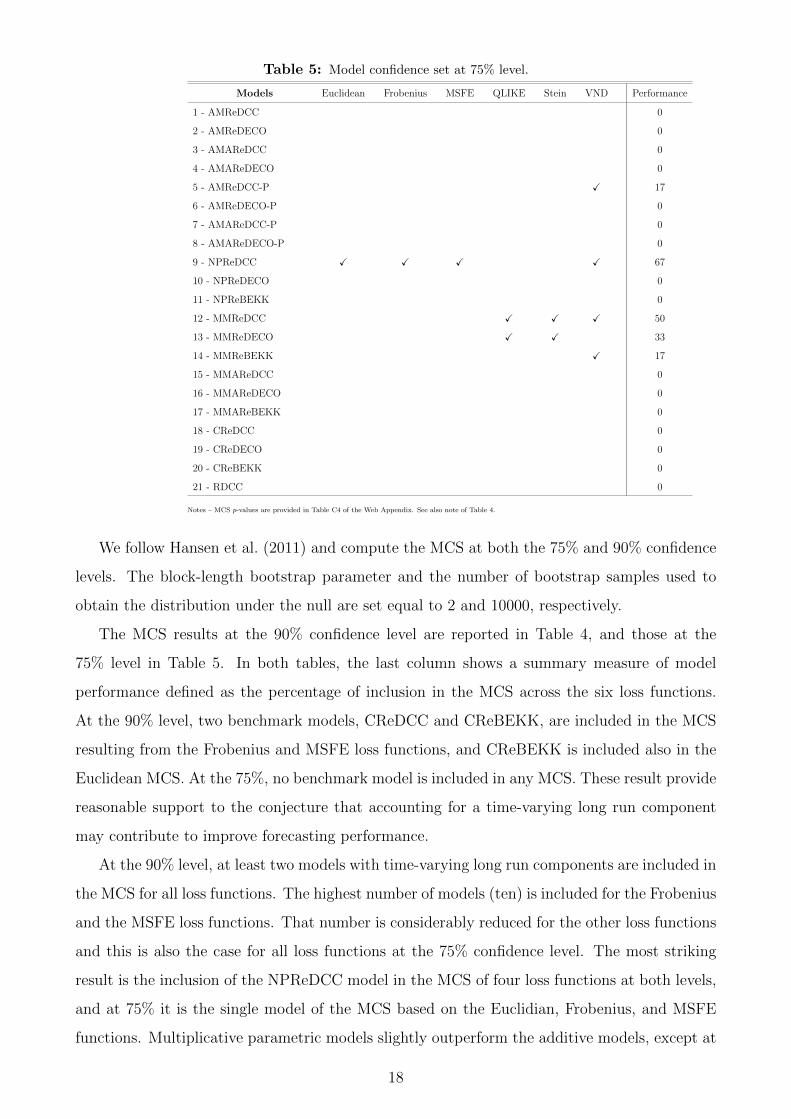
Table 5: Model confidence set at 75% level.
Models Euclidean Frobenius MSFE QLIKE Stein VND Performance
1 - AMReDCC 0
2 - AMReDECO 0
3 - AMAReDCC 0
4 - AMAReDECO 0
5 - AMReDCC-P X 17
6 - AMReDECO-P 0
7 - AMAReDCC-P 0
8 - AMAReDECO-P 0
9 - NPReDCC X X X X 67
10 - NPReDECO 0
11 - NPReBEKK 0
12 - MMReDCC X X X 50
13 - MMReDECO X X 33
14 - MMReBEKK X 17
15 - MMAReDCC 0
16 - MMAReDECO 0
17 - MMAReBEKK 0
18 - CReDCC 0
19 - CReDECO 0
20 - CReBEKK 0
21 - RDCC 0
Notes – MCS p-values are provided in Table C4 of the Web Appendix. See also note of Table 4.
We follow Hansen et al. (2011) and compute the MCS at both the 75% and 90% confidence
levels. The block-length bootstrap parameter and the number of bootstrap samples used to
obtain the distribution under the null are set equal to 2 and 10000, respectively.
The MCS results at the 90% confidence level are reported in Table 4, and those at the
75% level in Table 5. In both tables, the last column shows a summary measure of model
performance defined as the percentage of inclusion in the MCS across the six loss functions.
At the 90% level, two benchmark models, CReDCC and CReBEKK, are included in the MCS
resulting from the Frobenius and MSFE loss functions, and CReBEKK is included also in the
Euclidean MCS. At the 75%, no benchmark model is included in any MCS. These result provide
reasonable support to the conjecture that accounting for a time-varying long run component
may contribute to improve forecasting performance.
At the 90% level, at least two models with time-varying long run components are included in
the MCS for all loss functions. The highest number of models (ten) is included for the Frobenius
and the MSFE loss functions. That number is considerably reduced for the other loss functions
and this is also the case for all loss functions at the 75% confidence level. The most striking
result is the inclusion of the NPReDCC model in the MCS of four loss functions at both levels,
and at 75% it is the single model of the MCS based on the Euclidian, Frobenius, and MSFE
functions. Multiplicative parametric models slightly outperform the additive models, except at
18

the 90% level for the Frobenius and MSFE functions. DCC and BEKK-type models are more
often selected than DECO-type models.
4.3.2 Out-of-sample hedging performance
In choosing among different competing models, practitioners are willing to employ the best
one whose performance can be evaluated in an economically meaningful way. In portfolio
management, for example, they are interested in the model providing portfolios with the lowest
variance among a set of models. We accomplish this kind of comparison adopting the method
proposed by Engle & Colacito (2006) pertaining to minimum variance portfolio management.
Namely, by using out-of-sample covariance forecasts from the set of competing models, we form
both global minimum variance (GMV) portfolios and minimum variance (MV) portfolios.
The GMV portfolio weights are obtained as solution to the optimization problem
minwt
w′tHtwt s.t.n∑j=1
wt,j = 1,
where wt is the vector of portfolio weights for time t chosen at time t − 1, Ht denotes the
conditional covariance forecast from a generic model, and the only requirement is on the vector
of weights to sum up to unity. The MV portfolio is achieved by adding an additional constraint
on the vector of expected returns µ, i.e. w′tµ ≥ q. As pointed out by Engle & Colacito (2006),
the portfolio volatility is smallest for the correctly specified covariance matrix for any vector
of expected returns. Hence, for computational ease, we set the conditional mean return vector
equal to the historical mean, and like Engle & Kelly (2012), we impose a target expected annual
return of 10%.
As a result, we get series of 712 out-of-sample GMV and MV daily portfolio returns and their
corresponding daily variances for each model. According to the initial statement, a superior
model is required to produce optimal portfolios with lower variance realizations. In order to
test for the significance of the differences between portfolio variances, we employ a Diebold
and Mariano (2002) test between the overall best performing model among the 21 models
and the first best model in the benchmark group. Table 6 reports standard deviations of
the forecasted portfolio returns time series along with each model position in the ranking.
Results for the GMV portfolios are shown in the second column of the table. Noticeably,
there are no benchmark models up to the eighth position. The five best performing models
belong to the multiplicative class, and the MMReDCC achieves the lowest variance GMV
portfolio with a standard deviation of 1.0711. This improves at the 1% significance level over
the first best benchmark, the CReDCC, which achieves a standard deviation of 1.0815. A
19

plausible reason for this difference stems from the comparison of the correlations extracted from
both models, as shown in Figure 4. Apparently, the CReDCC model tends to underestimate
correlations especially during the higher volatile period, thus leading to a less appreciable gain
from portfolio diversification. The other constant long term models have broadly the same
2007 2008 2009 2010
0
1
MMReDCC − Conditional correlation (JPM−XOM)
CReDCC − Conditional correlation (JPM−XOM)
Figure 4: Comparison of predicted correlations of JPM-XOM stock from MMReDCC and CReDCC models
inferior performance, except that the CReBEKK model slightly improves over its competitors
involving a BEKK-type structure. Not really surprisingly, as it reminds the finding obtained
in the MCS evaluation, the RDCC closes the ranking with the highest standard deviation of
1.1218. Similar results are found for the MV portfolios in the fourth column. The MMReDCC
model confirms its predominance (1.0958) and significantly improves over the first best constant
long run model (CReBEKK, 1.1102) at the 1% significance level. The other benchmarks are
all ranked in the last positions.
Briefly, we can interpret minimum variance portfolio results from this forecasting exercise as
providing clear evidence that there can be hedging benefits from employing models that account
for a time-varying long run component. In some cases, these benefits can be remarkable,
depending on the chosen long run component-type structure or the short run multivariate
specification.
4.3.3 Portfolio VaR forecasting
In this last application, we consider the forecasting of portfolio Value-at-Risk (VaR). The aim is
to study the possible efficiency gain of using the time-varying long run component models over
benchmarks for one-step-ahead VaR predictions. Our analysis is concerned with the forecasting
of the long side of the daily VaR. This corresponds to the VaR level for traders having long
positions in their asset holdings, and thus the predictive power of a specific model is related
to its ability to model large negative returns. For simplicity, we abstract from the Markovitz
20

Table 6: Out-of-sample hedging performance
Models GMV MV
std. rank std. rank
1 - AMReDCC 1.07963 (7) 1.10497 (8)
2 - AMReDECO 1.08335 (9) 1.11160 (14)
3 - AMAReDCC 1.08545 (13) 1.11072 (13)
4 - AMAReDECO 1.08672 (15) 1.11683 (15)
5 - AMReDCC-P 1.07792 (6) 1.10341 (6)
6 - AMReDECO-P 1.08590 (14) 1.11440 (16)
7 - AMAReDCC-P 1.08487 (12) 1.10968 (10)
8 - AMAReDECO-P 1.08782 (16) 1.11441 (17)
9 - NPReDCC 1.07190 (2) 1.09910 (4)
10 - NPReDECO 1.08404 (11) 1.10465 (7)
11 - NPReBEKK 1.11439 (20) 1.13175 (20)
12 - MMReDCC 1.0711∗∗
(1) 1.0958∗∗
(1)
13 - MMReDECO 1.07307 (3) 1.09874 (3)
14 - MMReBEKK 1.08886 (18) 1.10897 (9)
15 - MMAReDCC 1.07308 (4) 1.09687 (2)
16 - MMAReDECO 1.07790 (5) 1.10264 (5)
17 - MMAReBEKK 1.08958 (19) 1.11053 (12)
18 - CReDCC 1.08149 (8) 1.11168 (18)
19 - CReDECO 1.08357 (10) 1.13073 (19)
20 - CReBEKK 1.08858 (17) 1.11026 (11)
21 - RDCC 1.12175 (21) 1.14693 (21)
Notes – The table reports standard deviations of the portfolios return time series. The best performing model in each column is in
bold. A Diebold-Mariano test is performed to compare the variances achieved by the best model against the first best performing
model within the benchmarks in the same column. The best model is accompanied by * or ** if the difference is significant at the
5% or 1% level, respectively.
optimization setting employed in the previous application, considering only equally-weighted
portfolios.
For each model, the portfolio VaR at level α on day t, conditional on the information
available at time t− 1, is computed as:
V aRt(α) = zα√w′Htw,
where w is the given n-dimensional vector of equal weights, Ht is the forecasted conditional
covariance matrix for a generic model, and zα is the α% left-quantile of the standard normal
distribution. The same analysis was done assuming the more flexible Student distribution,
but as this did not lead to significant improvements, results are not reported. VaR at levels
α equal to 5%, 2.5% and 1% are forecasted, and their performance is then assessed using two
statistical backtesting methods. First, the Likelihood Ratio Conditional Coverage (LRcc) test
21

of Christoffersen (1998) is used; its construction relies on the so-called hit function, or indicator
function, obtained as follows:
It(α) =
1 if w′rt ≤ V aRt(α)
0 if w′rt > V aRt(α).
According to Finger (2005), good VaR models are capable of reacting to changing volatility
and correlations in a way that exceptions occur independently of each other, whereas bad
models tend to produce a sequence of consecutive exceptions. Christoffersen’s test accounts for
both properties of a good VaR model, namely the correct failure rate and the independence of
exceptions. The LRcc test statistic is χ21 distributed. The second method is the regression-based
test of Engle & Manganelli (2004), also known as the Dynamic Quantile (DQ) test. Instead
of directly considering the hit sequence, the test is based on its associated quantile process
Ht(α) = It(α)− α, formally expressed as
Ht(α) =
1− α if It = 1
−α if It = 0.
Its purpose it to link the current margin exceedances to past violations or past information
and subsequently testing for different restrictions on the parameters of the regression. We run
the regression Ht(α) = δ +K∑k=1
βkHt−k(α) + εt for K = 3 and we test the joint hypothesis
H0(DQcc) : δ = β1 = ... = βK = 0. This assumption coincides with the null of Christoffersen’s
LRcc test. It is also possible to split the test and separately test the independence hypothesis
and the unconditional coverage hypothesis, respectively as H0(DQind) : β1 = ... = βK = 0
and H0(DQuc) : δ = 0. Empirical results from the tests are given in Table 7. For each VaR
level, we report test statistics along with the corresponding p-values. The first column of each
panel depicts the results for the LRcc test while the last three columns show the results for
the DQuc, DQind and DQcc tests. Across the different VaR panels, the LRcc and DQcc tests
basically tell the same story. Rejections of the first test at the 5% level correspond to rejections
of the second, with very few exceptions.
Of main interest, the last four rows of the table report test statistics and p-values from
the benchmark models. Results are quite homogeneous among the three VaR panels and, at
least for the multiplicative models, they are considerably inferior to those obtained by the
corresponding time-varying counterparts.
Irrespective of their model structure, the tests for the benchmark models lead to rejections
in a vast majority of cases. On the contrary, the tests for the multiplicative component models
show a remarkably better performance. Both the nonparametric and the parametric versions
22

pass all the tests for α = 5% showing occasional rejections of the DQuc test for the most ex-
treme quantiles. Apparently, the flexibility of the multiplicative structure allows to adequately
model the left tail of the distribution and to deliver superior VaR forecasts. This holds for any
type of short term (DCC, BEKK DECO) specification.
It clearly appears that the additive class fails in predicting the VaR adequately. This is par-
ticularly visible for the 5% VaR, where the p-values for the null hypothesis of the various tests
are often smaller than 0.05 for most models.
However, by looking at the results of the DQind test across the board, violations do not
appear to be dependent. For VaR at levels α = 2.5% and α = 1%, models including a DCC
specification show a slight improvement in capturing the conditional coverage of both tests,
but the additive class still appears to be almost uniformly rejected. The only exception is the
AMAReDCC model, which passes all the tests with a single rejection at the 5% level for the
1% VaR.
The conclusion that can be drawn is that, for equally weighted portfolios, reliable VaR
forecasts can be obtained under the simple assumption of conditionally normally standardized
portfolio returns, by using time-varying long run component models that include an appropri-
ately chosen long term structure.
5 Conclusions
We propose a new set of component models allowing for time variation in the long run levels
of realized variances and correlations. Our modeling framework allows for the secular compo-
nent to enter the model structure either in additive fashion, as a time-varying intercept in the
conditional correlation model, or as a multiplicative factor. In the latter case, it is specified
parametrically, using a MIDAS specification, or non-parametrically, by means of a matrix-
variate smoother.
As a general finding, additive-type models have good in-sample fits while multiplicative models
tend to be preferred out-of-sample. In all cases, the choice of the multivariate GARCH speci-
fication plays a crucial role for accurately modeling the short-term dynamics and, among the
three possibilities proposed, the DCC appears to be prevailing.
In the empirical application we illustrate the potential benefits of using a time-varying long run
component instead of a constant one. When the dimension of the application is moderately
small, such as ten assets, estimation can be performed by maximizing a Wishart quasi likelihood
function in one step. This yields computationally tractable, consistent and asymptotically
23

Tab
le7:
Lik
elih
ood
Rati
oT
est
an
dD
yn
am
icQ
uanti
leT
est
Res
ult
s
VaR
1%
VaR
2.5
%V
aR
5%
Mod
els
LR
DQ
LR
DQ
LR
DQ
cc
uc
ind
cc
cc
uc
ind
cc
cc
uc
ind
cc
1-
AM
ReD
CC
3.94
(0.1
4)
5.0
9(0
.02)
0.44
(0.5
0)
5.3
0(0
.07)
2.65
(0.2
7)3.2
2(0
.07)
1.31
(0.2
5)
4.3
2(0
.11)
8.1
8(0
.02)
8.55
(0.0
0)
1.42
(0.2
3)
9.43
(0.0
1)
2-
AM
ReD
EC
O8.2
6(0
.02)
11.6
0(0
.00)
0.8
4(0
.36)
12.
10(
0.0
0)
2.65
(0.2
6)3.2
2(0
.07)
1.31
(0.2
5)
4.3
2(0
.11)
10.2
0(0
.01)
8.90
(0.0
0)
3.40
(0.0
6)
11.
44(0
.00)
3-
AM
AR
eDC
C2.8
0(0
.24)
3.50
(0.0
6)
0.3
5(0
.55)
3.74
(0.1
5)2.
00
(0.3
6)2.3
8(0
.12)
1.16
(0.2
8)
3.3
9(0
.18)
5.5
1(0
.07)
5.65
(0.0
2)
0.87
(0.3
5)
6.23
(0.0
5)
4-
AM
AR
eDE
CO
6.68
(0.0
4)
9.1
7(0
.00)
0.6
8(0
.41)
9.3
5(0
.01)
4.22
(0.1
2)5.2
8(0
.02)
1.6
6(0
.20)
6.57
(0.0
4)
8.1
8(0
.02)
8.55
(0.0
0)
1.42
(0.2
3)
9.43
(0.0
1)
5-
AM
ReD
CC
-P1.8
3(0
.40)
2.2
1(0
.14)
0.2
7(0
.60)
2.41
(0.3
0)2.
65
(0.2
6)3.2
2(0
.07)
1.31
(0.2
5)
4.3
2(0
.11)
7.2
4(0
.03)
7.52
(0.0
1)
1.22
(0.2
7)
8.29
(0.0
2)
6-
AM
ReD
EC
O-P
6.6
8(0
.04)
9.17
(0.0
0)
0.6
8(0
.41)
9.53
(0.0
1)
2.65
(0.2
7)3.2
2(0
.07)
1.31
(0.2
5)
4.3
2(0
.11)
12.4
0(0
.00)
11.2
0(0
.00)
0.13
(0.7
1)
14.
13(0
.00)
7-
AM
AR
eDC
C-P
3.9
4(0
.14)
5.0
9(0
.02)
0.4
4(0
.51)
5.37
(0.0
7)
2.01
(0.3
7)2.3
9(0
.12)
1.16
(0.2
8)
3.3
9(0
.18)
5.5
2(0
.06)
5.65
(0.0
2)
0.87
(0.3
4)
6.23
(0.0
4)
8-
AM
AR
eDE
CO
-P6.6
8(0
.04)
9.17
(0.0
0)
0.6
8(0
.41)
9.53
(0.0
1)
3.40
(0.1
8)4.1
8(0
.04)
1.4
8(0
.22)
5.38
(0.0
7)
9.0
7(0
.01)
10.4
2(0
.00)
0.51
(0.4
7)
10.
59(0
.01)
9-
NP
ReD
CC
1.8
3(0
.40)
2,2
1(0
.13)
0.2
7(0
.60)
2.41
(0.2
9)4.
22
(0.1
2)5.2
8(0
.02)
1.6
6(0
.19)
6.57
(0.0
4)
3.5
1(0
.17)
3.88
(0.0
5)
0.0
1(0
.94)
3.88
(0.1
4)
10
-N
PR
eDE
CO
3.9
4(0
.13)
5.09
(0.0
2)
0.4
4(0
.50)
5.37
(0.0
7)
1.42
(0.4
9)1.6
7(0
.19)
1.02
(0.3
1)
2.5
9(0
.27)
2.7
3(0
.25)
2.74
(0.0
9)
0.3
6(0
.54)
3.00
(0.2
2)
11
-N
PR
eBE
KK
3.8
4(0
.14)
1.83
(0.1
7)
6.4
2(0
.01)
8.5
7(0
.01)
4.22
(0.1
2)4.8
9(0
.03)
0.0
0(0
.97)
4.91
(0.0
9)
4.1
8(0
.12)
2.87
(0.0
9)
1.7
0(0
.19)
4.35
(0.1
1)
12
-M
MR
eDC
C1.8
3(0
.40)
2.2
1(0
.14)
0.2
7(0
.60)
2.41
(0.2
9)0.
55
(0.7
6)0.6
3(0
.42)
0.77
(0.
37)
1.3
7(0
.50)
5.6
5(0
.06)
3.74
(0.0
5)
2.1
2(0
.14)
6.01
(0.0
5)
13
-M
MR
eDE
CO
0.1
0(0
.95)
0.1
1(0
.73)
0.1
0(0
.74)
0.21
(0.8
9)0.
94
(0.6
2)1.0
9(0
.29)
0.89
(0.3
4)
1.9
2(0
.38)
4.1
8(0
.12)
2.87
(0.0
9)1.
70(0
.19)
4.3
5(0
.11)
14
-M
MR
eBE
KK
1.0
4(0
.59)
1.2
1(0
.27)
0.2
0(0
.65)
1.38
(0.5
0)2.
65
(0.2
7)3.2
2(0
.07)
1.31
(0.2
5)
4.3
2(0
.11)
2.7
3(0
.25)
2.74
(0.0
9)
0.3
5(0
.55)
3.00
(0.2
2)
15
-M
MA
ReD
CC
2.8
0(0
.24)
3.5
0(0
.06)
0.3
5(0
.55)
3.74
(0.1
5)0.
56
(0.7
6)0.6
3(0
.43)
0.77
(0.3
8)
1.3
7(0
.50)
4.1
9(0
.12)
2.87
(0.0
9)
1.7
0(0
.19)
4.35
(0.1
1)
16
-M
MA
ReD
EC
O1.0
4(0
.59)
1.2
1(0
.27)
0.2
0(0
.65)
1.3
8(0
.50)
0.94
(0.6
2)1.0
9(0
.29)
0.89
(0.3
5)
1.9
2(0
.38)
4.1
8(
0.1
2)2.
87(0
.09)
1.7
0(0
.19)
4.35
(0.1
1)
17
-M
MA
ReB
EK
K1.8
3(0
.40)
2.2
1(0
.13)
0.2
7(0
.60)
2.4
1(0
.29)
2.65
(0.2
7)3.2
2(0
.07)
1.31
(0.2
5)
4.3
3(0
.11)
1.5
1(0
.46)
0.62
(0.4
3)
0.8
7(0
.35)
1.45
(0.4
8)
18
-C
ReD
CC
9.97
(0.0
1)
14.4
6(0
.00)
1.0
0(0
.31)
14.
90(0
.00)
13.3
6(0
.00)
18.7
0(0
.00)
3.6
5(0
.05)
20.
77(0
.00)
14.6
2(0
.00)
17.1
9(0
.00)
1.39
(0.2
3)
17.
68(0
.00)
19
-C
ReD
EC
O24
.90
(0.0
0)
42.6
7(0
.00)
2.8
5(0
.09)
43.
40(0
.00)
30.1
5(0
.00)
47.5
6(0
.00)
7.8
9(0
.01)
50.
66(0
.00)
35.0
3(0
.00)
45.9
7(0
.00)
2.31
(0.1
2)
46.
09(0
.00)
20
-C
ReB
EK
K1.8
3(0
.40)
2.2
1(0
.13)
0.2
7(0
.60)
8.81
(0.0
3)
4.22
(0.1
2)5.2
8(0
.02)
1.6
6(0
.19)
6.57
(0.0
3)
5.5
1(0
.06)
5.65
(0.0
1)
0.87
(0.3
4)
6.23
(0.0
4)
21
-R
DC
C5.
23(0
.07)
6.9
8(0
.01)
0.5
5(0
.45)
7.30
(0.0
2)
9.43
(0.0
1)
12.6
8(0
.00)
2.7
8(0
.09)
14.
46(0
.00)
18.5
2(0
.00)
22.1
2(0
.00)
2.15
(0.1
4)
22.
80(0
.00)
Note
s–
Th
eta
ble
rep
ort
ste
stst
ati
stic
sof
the
Lik
elih
ood
Rati
o(L
R)
Con
dit
ion
al
Cover
age
Tes
tan
dof
the
Dyn
am
icQ
uanti
le(U
nco
nd
itio
nal
Cover
age,
Ind
epen
den
cean
dC
on
dit
ion
al
Cover
age)
test
for
the
equ
al
wei
ghte
dp
ort
folios
Valu
e-at-
Ris
kat
con
fid
ence
level
sα
=1%
,2.5
%an
d5%
.C
orr
esp
on
din
gp
-valu
esin
bra
cket
s;p
-valu
esin
bold
den
ote
sign
ifica
nce
at
the
5%
level
.
24

efficient estimates of the parameters. Estimation results show that time varying component
models deliver better full-sample likelihood fits as well as lower AIC and BIC values.
Their forecasting ability is then compared by means of three applications. Firstly, the MCS
approach is used to identify the best performing models given a set of consistent loss functions.
Results are in favour of the time-varying long run models, especially at the 75% MCS, as none
of the benchmarks is included. Secondly, we construct (global) minimum variance portfolios
to assess the models out-of-sample hedging performance. Again, constant long run models
are often outperformed, suggesting that there can be hedging benefits from employing models
which account for a time-varying long run component. Last, we forecast 1%, 2.5% and 5%
Value-at-Risk assuming equally weighted portfolios under the assumption of standard normal
quantiles. The benchmark models appear to deliver VaR forecasts that are considerably inferior
to those obtained by their corresponding more flexible counterparts.
Overall, our empirical results provide some evidence in favour of the hypothesis that ac-
counting for time variation in levels of volatilities and correlations contributes both to improve
in-sample fit and to provide more accurate out-of-sample one-step ahead forecasts.
References
Aıt-Sahalia, Y., Mykland, P. A. & Zhang, L. (2005), ‘How often to sample a continuous-
time process in the presence of market microstructure noise’, Review of Financial Studies
18(2), 351–416.
Andersen, T. G., Bollerslev, T., Diebold, F. X. & Labys, P. (2003), ‘Modeling and forecasting
realized volatility’, Econometrica 71(2), 579–625.
Anderson, T. (1984), An Introduction to Multivariate Statistical Analysis, second edn, Wiley.
Barndorff-Nielsen, O. E., Hansen, P. R., Lunde, A. & Shephard, N. (2009), ‘Realized kernels
in practice: Trades and quotes’, The Econometrics Journal 12(3), C1–C32.
Barndorff-Nielsen, O. & Shephard, N. (2001), ‘Normal modified stable processes’, Theory of
Probability and Mathematics Statistics 65, 1–19.
Bauwens, L., Hafner, C. M. & Pierret, D. (2013), ‘Multivariate volatility modeling of electricity
futures’, Journal of Applied Econometrics 28(5), 743–761.
Bauwens, L., Storti, G. & Violante, F. (2012), Dynamic conditional correlation models for
realized covariance matrices. CORE DP 2012/60.
25

Chiriac, R. & Voev, V. (2011), ‘Modelling and forecasting multivariate realized volatility’,
Journal of Applied Econometrics 26, 922–947.
Christoffersen, P. F. (1998), ‘Evaluating interval forecasts’, International Economic Review
pp. 841–862.
Colacito, R., Engle, R. F. & Ghysels, E. (2011), ‘A component model for dynamic correlations’,
Journal of Econometrics 164(1), 45–59.
Engle, R. (2002), ‘Dynamic conditional correlation: A simple class of multivariate general-
ized autoregressive conditional heteroskedasticity models’, Journal of Business & Economic
Statistics 20(3), 339–350.
Engle, R. & Colacito, R. (2006), ‘Testing and valuing dynamic correlations for asset allocation’,
Journal of Business & Economic Statistics 24(2), 238–253.
Engle, R., Ghysels, E. & Sohn, B. (2008), On the economic sources of stock market volatility,
in ‘AFA 2008 New Orleans Meetings Paper’.
Engle, R. & Kelly, B. (2012), ‘Dynamic equicorrelation’, Journal of Business & Economic
Statistics 30, 212–228.
Engle, R. & Lee, G. (1999), A Permanent and Transitory Component Model of Stock Return
Volatility, Cointegration, Causality, and Forecasting: A Festschrift in Honor of Clive W.J.
Granger, Oxford University Press - R. Engle and H. White eds., pp. 475–497.
Engle, R. & Manganelli, S. (2004), ‘Caviar: Conditional autoregressive value at risk by regres-
sion quantiles’, Journal of Business & Economic Statistics 22(4), 367–381.
Engle, R. & Rangel, J. (2008), ‘The spline-GARCH model for low-frequency volatility and its
global macroeconomic causes’, Review of Financial Studies 21(3), 1187–1222.
Finger, C. (2005), ‘Back to backtesting’, RiskMetrics Monthly Research .
Golosnoy, V., Gribisch, B. & Liesenfeld, R. (2012), ‘The conditional autoregressive wishart
model for multivariate stock market volatility’, Journal of Econometrics 167(1), 211–223.
Gourieroux, C., Jasiak, J. & Sufana, R. (2009), ‘The wishart autoregressive process of multi-
variate stochastic volatility’, Journal of Econometrics 150(2), 167–181.
Hafner, C. & Linton, B. (2010), ‘Efficient estimation of a multivariate multiplicative volatility
model’, Journal of Econometrics 159(1), 55–73.
26

Hansen, P. R., Lunde, A. & Nason, J. M. (2011), ‘The model confidence set’, Econometrica
79(2), 453–497.
Hardle, W. (2004), Nonparametric and semiparametric models, Springer.
Jin, X. & Maheu, J. M. (2013), ‘Modeling realized covariances and returns’, Journal of Financial
Econometrics 11(2), 335–369.
Laurent, S., Rombouts, J. V. & Violante, F. (2013), ‘On loss functions and ranking forecasting
performances of multivariate volatility models’, Journal of Econometrics 173(1), 1–10.
Noureldin, D., Shephard, N. & Sheppard, K. (2012), ‘Multivariate high-frequency-based volatil-
ity (heavy) models’, Journal of Applied Econometrics 27, 907–933.
Patton, A. J. (2011), ‘Volatility forecast comparison using imperfect volatility proxies’, Journal
of Econometrics 160(1), 246–256.
Patton, A. J. & Sheppard, K. (2009), ‘Optimal combinations of realised volatility estimators’,
International Journal of Forecasting 25(2), 218–238.
Rice, J. (1984), ‘Bandwidth choice for nonparametric regression’, The Annals of Statistics
12(4), 1215–1230.
Tse, Y. & Tsui, A. (2002), ‘A multivariate garch model with time-varying correlations’, Journal
of Business & Economic Statistics 20(3), 351–362.
Zhang, L. (2011), ‘Estimating covariation: Epps effect, microstructure noise’, Journal of Econo-
metrics 160(1), 33–47.
27

Web Appendix to
Forecasting Comparison of Long Term Component
Dynamic Models For Realized Covariance Matrices
November 19, 2014
Luc Bauwens1
Universite catholique de Louvain,CORE, B-1348 Louvain-La-Neuve, Belgium;
University of Johannesburg,Department of Economics and Econometrics, Johannesburg, South Africa.
Manuela Braione1
Universite catholique de Louvain,CORE, B-1348 Louvain-La-Neuve, Belgium
Giuseppe StortiUniversita di Salerno
Department of Economics and Statistics, Fisciano, [email protected]
Keywords: Realized covariance, component dynamic models, MIDAS, minimum variance
portfolio, model confidence set, Value-at-Risk.
JEL Classification: C13, C32, C58.
1Luc Bauwens and Manuela Braione acknowledge support of the ”Communaute francaise de Belgique”through contract ”Projet d’Actions de Recherche Concertees” 12/17-045”, granted by the ”Academie uni-versitaire Louvain”.

Appendix A Descriptive statistics
Table A1: Descriptive statistics of realized variances.
Stock Mean Max. Min. Std.dev. Skewness Kurtosis
Estimation sample: February 1, 2001 to December 31, 2006 (1528 observations)
BAC 1.31 19.35 0.07 1.88 4.66 32.54
JPM 2.88 168.72 0.11 6.45 14.86 329.89
IBM 1.60 40.69 0.08 2.27 6.23 73.62
MSFT 2.19 29.65 0.10 2.86 3.98 26.93
XOM 1.59 40.89 0.13 1.98 8.29 126.45
AA 2.85 30.57 0.29 2.71 3.71 24.24
AXP 2.33 62.94 0.08 4.01 6.23 65.13
DD 1.83 28.93 0.16 2.07 4.98 46.68
GE 1.98 55.74 0.10 3.06 6.49 80.14
KO 1.29 22.21 0.04 1.60 5.57 52.96
Forecasting sample: January 1, 2007 to December 31, 2009 (712 observations)
BAC 14.36 277.31 0.10 27.69 4.07 25.22
JPM 9.74 176.48 0.16 16.32 4.74 34.81
IBM 2.65 57.54 0.10 4.88 5.86 49.89
MSFT 3.02 43.11 0.08 4.32 4.65 31.49
XOM 3.12 115.38 0.17 6.66 9.28 129.77
AA 9.44 160.24 0.49 14.36 4.82 36.89
AXP 8.91 201.88 0.24 14.14 6.09 64.94
DD 4.02 63.87 0.17 5.60 4.75 35.36
GE 5.81 114.26 0.18 11.37 4.66 31.05
KO 1.69 56.51 0.12 3.23 8.79 125.68
Full sample: February 1, 2001 to December 31, 2009 (2240 observations)
BAC 5.46 277.31 0.07 16.82 7.17 72.51
JPM 5.06 176.48 0.11 11.10 7.53 84.62
IBM 1.93 57.54 0.08 3.36 7.32 84.96
MSFT 2.45 43.11 0.08 3.41 4.73 36.29
XOM 2.07 115.38 0.13 4.16 13.29 287.87
AA 4.95 160.24 0.29 8.94 7.63 92.05
AXP 4.42 201.88 0.08 9.16 8.53 133.60
DD 2.53 63.87 0.16 3.73 6.44 68.47
GE 3.20 114.26 0.10 7.12 7.23 75.42
KO 1.41 56.51 0.04 2.26 9.71 180.08
Notes – Descriptive statistics of the realized variances of the stocks used in the empirical application. The three panels report the
statistics for the in-sample period, the out-of-sample period and the full sample period, respectively.
28
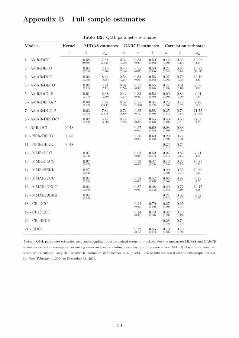
Appendix B Full sample estimates
Table B2: QML parameter estimates
Models Kernel MIDAS estimates GARCH estimates Correlation estimates
h θ ω2s m γ δ α β ω2r
1 - AMReDCC 0.68(0.080)
7.51(2.506)
0.34(0.09)
0.33(0.03)
0.50(0.06)
0.12(0.00)
0.56(0.15)
12.05(2.84)
2 - AMReDECO 0.64(0.30)
7.19(3.20)
0.40(0.46)
0.35(0.05)
0.50(0.09)
0.24(0.04)
0.63(0.18)
10.73(14.47)
3 - AMAReDCC 0.02(0.00)
8.34(8.55)
0.53(0.35)
0.33(0.04)
0.56(0.08)
0.27(0.06)
0.70(0.08)
12.10(3.83)
4 - AMAReDECO 0.02(0.01)
4.91(5.11)
0.67(0.50)
0.37(0.04)
0.55(0.05)
0.47(0.09)
0.51(0.10)
20.6(9.93)
5 - AMReDCC-P 0.61(0.11)
6.68(2.50)
0.42(0.13)
0.33(0.03)
0.52(0.06)
0.09(0.00)
0.89(0.00)
2.91(1.44)
6 - AMReDECO-P 0.60(0.27)
7.84(16.40)
0.52(0.28)
0.35(0.053)
0.44(0.12)
0.25(0.05)
0.70(0.07)
2.46(11.2)
7 - AMAReDCC-P 0.03(0.01)
7.84(23.78)
0.72(1.89)
0.35(0.12)
0.58(0.09)
0.25(0.11)
0.73(0.13)
11.75(24.29)
8 - AMAReDECO-P 0.02(0.00)
5.42(7.30)
0.74(0.19)
0.37(0.03)
0.55(0.06)
0.40(0.19)
0.60(0.21)
27.30(9.29)
9 - NPReDCC 0.078 0.37(0.03)
0.60(0.04)
0.08(0.00)
0.88(0.00)
10 - NPReDECO 0.078 0.36(0.03)
0.60(0.04)
0.20(0.02)
0.74(0.03)
11 - NPReBEKK 0.078 0.23(0.01)
0.74(0.01)
12 - MMReDCC 0.97(0.42)
0.23(0.04)
0.50(0.17)
0.07(0.01)
0.82(0.14)
7.21(2.80)
13 - MMReDECO 0.97(0.07)
0.39(0.09)
0.47(0.13)
0.19(0.08)
0.72(0.13)
13.87(1.72)
14 - MMReBEKK 0.87(0.04)
0.20(0.02)
0.55(0.07)
19.89(7.63)
15 - MMAReDCC 0.04(0.00)
0.38(0.04)
0.52(0.05)
0.06(0.00)
0.87(0.01)
5.79(0.62)
16 - MMAReDECO 0.04(0.00)
0.37(0.05)
0.48(0.13)
0.20(0.08)
0.72(0.19)
12.17(5.48)
17 - MMAReBEKK 0.04(0.00)
0.24(0.01)
0.62(0.02)
8.62(1.01)
18 - CReDCC 0.22(0.02)
0.70(0.02)
0.27(0.00)
0.65(0.01)
19 - CReDECO 0.14(0.05)
0.79(0.10)
0.32(0.09)
0.70(0.19)
20 - CReBEKK 0.28(0.03)
0.74(0.03)
21 - RDCC 0.32(0.12)
0.56(0.21)
0.19(0.08)
0.70(0.09)
Notes – QML parameter estimates and corresponding robust standard errors in brackets. For the univariate MIDAS and GARCH
estimates we report average values among series and corresponding mean asymptotic square errors (MASE). Asymptotic standard
errors are calculated using the ”sandwich” estimator of Bollerslev et al.(1988). The results are based on the full-sample dataset,
i.e. from February 1, 2001 to December 31, 2009.
29

Appendix C Model Confidence Set
Appendix C.1 Loss functions
The set of robust loss functions used in the empirical application involves Euclidean and Frobe-
nius distances, Mean Square Forecast Error (MSFE), QLIKE, Stein and von Neumann diver-
gence (VND). Their definition is provided in the following table.
Loss Function Formula Type
Euclidean vech(
Σt −Ht
)′vech
(Σt −Ht
)Symmetric
Frobenius tr
[(Σt −Ht
)′ (Σt −Ht
)]Symmetric
MSFE 1T
vec(
Σt −Ht
)′vec(
Σt −Ht
)Symmetric
QLIKE log |Ht|+ vec(H−1t Σt
)′ι Symmetric
Stein tr(H−1t Σt)− log |H−1
t Σt| − n Asymmetric
VND tr(
Σt log Σt − Σt logHt − Σt +Ht
)Asymmetric
Notes – ι denotes a vector of ones, T is the out-of-sample length and n is the number of assets.
In the table, Σt is the proxy used for the true conditional covariance matrix while Ht denotes
each model predicted covariance matrix for the day t (the subscript i on Ht has been removed
for simplicity).
The first three loss functions are symmetric quadratic loss functions based on the forecast error.
The Euclidean distance only accounts for the unique elements of the covariance matrix while
the Frobenius distance double counts the loss associated to the conditional covariances.
The last two loss functions belong to the family of Bregman matrix divergences, which generalize
the squared Euclidean distance to a class of distances that all share similar properties. The
Stein loss function is scale invariant, being based on the standardized forecast error (in matrix
sense) and can be obtained as the objective function of the Wishart distribution, while the von
Neumann divergence is a matrix generalization of Kullback-Leibler divergence. Both Stein and
VND are asymmetric with respect to over/under predictions.
30

Appendix C.2 MCS p-values
Table C3: 90% MCS p-values
Models Euclidean Frobenius MSFE QLIKE Stein VND
1 - AMReDCC 0.0973 0.1799 0.1637 0.0067 0.0053 0.0987
2 - AMReDECO 0.0973 0.1799 0.1637 0.0000 0.0000 0.0000
3 - AMAReDCC 0.0973 0.1799 0.1637 0.0067 0.0001 0.0929
4 - AMAReDECO 0.0973 0.1799 0.1637 0.0000 0.0000 0.0000
5 - AMReDCC-P 0.0996 0.1927 0.1936 0.0067 0.0053 0.203
6 - AMReDECO-P 0.0608 0.1257 0.1214 0.0000 0.0000 0.0000
7 - AMAReDCC-P 0.0973 0.1799 0.1637 0.0003 0.0000 0.0929
8 - AMAReDECO-P 0.0608 0.0943 0.0854 0.0000 0.0000 0.0000
9 - NPReDCC 1.000 1.000 1.000 0.0000 0.0000 1.000
10 - NPReDECO 0.0608 0.0877 0.0854 0.0000 0.0000 0.0013
11 - NPReBEKK 0.0608 0.0943 0.0854 0.0000 0.0000 0.0013
12 - MMReDCC 0.0608 0.0943 0.0854 1.000 1.000 0.203
13 - MMReDECO 0.0608 0.0943 0.0854 0.2993 0.3005 0.0987
14 - MMReBEKK 0.1885 0.1927 0.1936 0.0000 0.0000 0.203
15 - MMAReDCC 0.0608 0.0943 0.0854 0.0067 0.0053 0.1612
16 - MMAReDECO 0.0608 0.0877 0.0854 0.0003 0.0001 0.0168
17 - MMAReBEKK 0.0996 0.1927 0.1936 0.0000 0.0000 0.0388
18 - CReDCC 0.0608 0.1257 0.1214 0.0000 0.0000 0.0168
19 - CReDECO 0.0608 0.0943 0.0854 0.0000 0.0000 0.0000
20 - CReBEKK 0.1885 0.206 0.1993 0.0000 0.0000 0.0987
21 - RDCC 0.0533 0.076 0.0697 0.0000 0.0000 0.0000
Notes – Entries are the p-values of the models included in the 90% MCS.
Table C4: 75% MCS p-values
Models Euclidean Frobenius MSFE QLIKE Stein VND
1 - AMReDCC 0.103 0.192 0.167 0.006 0.006 0.104
2 - AMReDECO 0.103 0.192 0.167 0.000 0.000 0.000
3 - AMAReDCC 0.103 0.192 0.167 0.006 0.006 0.094
4 - AMAReDECO 0.103 0.192 0.167 0.000 0.000 0.000
5 - AMReDCC-P 0.103 0.203 0.188 0.006 0.006 0.273
6 - AMReDECO-P 0.066 0.128 0.130 0.000 0.000 0.000
7 - AMAReDCC-P 0.103 0.192 0.167 0.001 0.001 0.094
8 - AMAReDECO-P 0.066 0.103 0.087 0.000 0.000 0.000
9 - NP-ReDCC 1.000 1.000 1.000 0.000 0.000 1.000
10 - NP-ReDECO 0.066 0.086 0.087 0.000 0.000 0.001
11 - NP-ReBEKK 0.066 0.103 0.087 0.000 0.000 0.001
12 - MMReDCC 0.066 0.103 0.087 1.000 1.000 0.273
13 - MMReDECO 0.066 0.103 0.087 0.309 0.289 0.104
14 - MMReBEKK 0.185 0.203 0.188 0.000 0.000 0.273
15 - MMAReDCC 0.066 0.103 0.087 0.006 0.006 0.181
16 - MMAReDECO 0.066 0.086 0.087 0.001 0.001 0.018
17 - MMAReBEKK 0.103 0.203 0.188 0.000 0.000 0.043
18 - CReDCC 0.066 0.128 0.130 0.000 0.000 0.018
19 - CReDECO 0.066 0.103 0.087 0.000 0.000 0.000
20 - CReBEKK 0.185 0.203 0.210 0.000 0.000 0.104
21 - RDCC 0.046 0.073 0.069 0.000 0.000 0.000
Notes – Entries are the p-values of the models included in the 75% MCS.
31

Recent titles CORE Discussion Papers
2014/11 Helmuth CREMER and Pierre PESTIEAU. Means-tested long term care and family transfers. 2014/12 Luc BAUWENS, Lyudmila GRIGORYEVA and Juan-Pablo ORTEGA. Estimation and
empirical performance of non-scalar dynamic conditional correlation models. 2014/13 Christian M. HAFNER and Arie PREMINGER. A note on the Tobit model in the presence of a
duration variable. 2014/14 Jean-François CARPANTIER and Arnaud DUFAYS. Specific Markov-switching behaviour for
ARMA parameters. 2014/15 Federico GRIGIS DE STEFANO. Strategic stability of equilibria: the missing paragraph. 2014/16 Claudio TELHA and Mathieu VAN VYVE. Efficient approximation algorithms for the
economic lot-sizing in continuous time. 2014/17 Yukai YANG. Testing constancy of the error covariance matrix in vector models against
parametric alternatives using a spectral decomposition. 2014/18 Koen DECANCQ, Marc FLEURBAEY and Erik SCHOKKAERT. Inequality, income, and
well-being. 2014/19 Paul BELLEFLAMME and Martin PEITZ. Digital piracy: an update. 2014/20 Eva-Maria SCHOLZ. Licensing to vertically related markets. 2014/21 N. Baris VARDAR. Optimal energy transition and taxation of non-renewable resources. 2014/22 Benoît DECERF. Income poverty measures with relative poverty lines. 2014/23 Antoine DEDRY, Harun ONDER and Pierre PESTIEAU. Aging, social security design and
capital accumulation. 2014/24 Biung-Ghi JU and Juan D. MORENO-TERNERO. Fair allocation of disputed properties. 2014/25 Nguyen Thang DAO. From agriculture to manufacture: How does geography matter ? 2014/26 Xavier Y. WAUTHY. From Bertrand to Cournot via Kreps and Scheinkman: a hazardous
journey. 2014/27 Gustavo BERGANTIÑOS and Juan MORENO-TERNERO. The axiomatic approach to the
problem of sharing the revenue from bundled pricing. 2014/28 Jean HINDRIKS and Yukihiro NISHIMURA. International tax leadership among asymmetric
countries. 2014/29 Jean HINDRIKS and Yukihiro NISHIMURA. A note on equilibrium leadership in tax
competition models. 2014/30 Olivier BOS and Tom TRUYTS. Auctions with prestige motives. 2014/31 Juan D. MORENO-TERNERO and Lars P. ØSTERDAL . Normative foundations for equity-
sensitive population health evaluation functions. 2014/32 P. Jean-Jacques HERINGS, Ana MAULEON and Vincent VANNETELBOSCH. Stability of
networks under Level-K farsightedness. 2014/33 Lionel ARTIGE, Laurent CAVENAILE and Pierre PESTIEAU. The macroeconomics of PAYG
pension schemes in an aging society. 2014/34 Tanguy KEGELART and Mathieu VAN VYVE. A conic optimization approach for SKU
rationalization. 2014/35 Ulrike KORNEK, Kei LESSMANN and Henry TULKENS. Transferable and non transferable
utility implementations of coalitional stability in integrated assessment models. 2014/36 Ibrahim ABADA, Andreas EHRENMANN and Yves SMEERS. Endogenizing long-term
contracts in gas market models. 2014/37 Julio DAVILA. Output externalities on total factor productivity. 2014/38 Diane PIERRET. Systemic risk and the solvency-liquidity nexus of banks. 2014/39 Paul BELLEFLAMME and Julien JACQMIN. An economic appraisal of MOOC platforms:
business models and impacts on higher education. 2014/40 Marie-Louise LEROUX, Pierre PESTIEAU and Grégory PONTHIERE. Longévité
différentielle et redistribution: enjeux théoriques et empiriques.

Recent titles CORE Discussion Papers - continued
2014/41 Chiara CANTA, Pierre PESTIEAU and Emmanuel THIBAULT. Long term care and capital
accumulation: the impact of the State, the market and the family. 2014/42 Gilles GRANDJEAN, Marco MANTOVANI, Ana MAULEON and Vincent
VANNETELBOSCH. Whom are you talking with ? An experiment on credibility and communication structure.
2014/43 Julio DAVILA. The rationality of expectations formation. 2014/44 Florian MAYNERIS, Sandra PONCET and Tao ZHANG. The cleaning effect of minimum
wages. Minimum wages, firm dynamics and aggregate productivity in China. 2014/45 Thierry BRECHET, Natali HRITONENKOVA and Yuri YATSENKO. Domestic
environmental policy and international cooperation for global commons. 2014/46 Mathieu PARENTI, Philip USHCHEV and Jacques-François THISSE. Toward a theory of
monopolistic competition. 2014/47 Takatoshi TABUCHI, Jacques-François THISSE and Xiwei ZHU. Does technological progress
affect the location of economic activity? 2014/48 Paul CASTANEDA DOWER, Victor GINSBURGH and Shlomo WEBER. Colonial legacy,
linguistic disenfranchisement and the civil conflict in Sri Lanka. 2014/49 Victor GINSBURGH, Jacques MELITZ and Farid TOUBAL. Foreign language learnings: An
econometric analysis. 2014/50 Koen DECANCQ and Dirk NEUMANN. Does the choice of well-being measure matter
empirically? An illustration with German data. 2014/51 François MANIQUET. Social ordering functions. 2014/52 Ivar EKELAND and Maurice QUEYRANNE. Optimal pits and optimal transportation. 2014/53 Luc BAUWENS, Manuela BRAIONE and Giuseppe STORTI. Forecasting comparison of long
term component dynamic models for realized covariance matrices.
Books V. GINSBURGH and S. WEBER (2011), How many languages make sense? The economics of linguistic
diversity. Princeton University Press. I. THOMAS, D. VANNESTE and X. QUERRIAU (2011), Atlas de Belgique – Tome 4 Habitat. Academia
Press. W. GAERTNER and E. SCHOKKAERT (2012), Empirical social choice. Cambridge University Press. L. BAUWENS, Ch. HAFNER and S. LAURENT (2012), Handbook of volatility models and their
applications. Wiley. J-C. PRAGER and J. THISSE (2012), Economic geography and the unequal development of regions.
Routledge. M. FLEURBAEY and F. MANIQUET (2012), Equality of opportunity: the economics of responsibility.
World Scientific. J. HINDRIKS (2012), Gestion publique. De Boeck. M. FUJITA and J.F. THISSE (2013), Economics of agglomeration: cities, industrial location, and
globalization. (2nd edition). Cambridge University Press. J. HINDRIKS and G.D. MYLES (2013). Intermediate public economics. (2nd edition). MIT Press. J. HINDRIKS, G.D. MYLES and N. HASHIMZADE (2013). Solutions manual to accompany intermediate
public economics. (2nd edition). MIT Press.
CORE Lecture Series R. AMIR (2002), Supermodularity and complementarity in economics. R. WEISMANTEL (2006), Lectures on mixed nonlinear programming. A. SHAPIRO (2010), Stochastic programming: modeling and theory.


![K-Regret Queries: From Additive to Multiplicative Utilities · arXiv:1609.07964v3 [cs.DB] 1 Oct 2016 K-Regret Queries: From Additive to Multiplicative Utilities Jianzhong Qi1, Fei](https://img.pdfslide.us/doc/110x75/5ac1f9f07f8b9a357e8d51e6/k-regret-queries-from-additive-to-multiplicative-utilities-160907964v3-csdb.jpg)