DISCUSSION PAPER SERIES

ABCD

www.cepr.org

Available online at: www.cepr.org/pubs/dps/DP9115.asp www.ssrn.com/xxx/xxx/xxx

No. 9115

TAXATION AND LABOR SUPPLY OF MARRIED WOMEN ACROSS

COUNTRIES: A MACROECONOMIC ANALYSIS

Alexander Bick and Nicola Fuchs-Schündeln

INTERNATIONAL MACROECONOMICS

ISSN 0265-8003

TAXATION AND LABOR SUPPLY OF MARRIED WOMEN ACROSS COUNTRIES: A

MACROECONOMIC ANALYSIS

Alexander Bick, Arizona State University Nicola Fuchs-Schündeln, Goethe University Frankfurt and CEPR

Discussion Paper No. 9115 September 2012

Centre for Economic Policy Research 77 Bastwick Street, London EC1V 3PZ, UK

Tel: (44 20) 7183 8801, Fax: (44 20) 7183 8820 Email: cepr@cepr.org, Website: www.cepr.org

This Discussion Paper is issued under the auspices of the Centre’s research programme in INTERNATIONAL MACROECONOMICS. Any opinions expressed here are those of the author(s) and not those of the Centre for Economic Policy Research. Research disseminated by CEPR may include views on policy, but the Centre itself takes no institutional policy positions.

The Centre for Economic Policy Research was established in 1983 as an educational charity, to promote independent analysis and public discussion of open economies and the relations among them. It is pluralist and non-partisan, bringing economic research to bear on the analysis of medium- and long-run policy questions.

These Discussion Papers often represent preliminary or incomplete work, circulated to encourage discussion and comment. Citation and use of such a paper should take account of its provisional character.

Copyright: Alexander Bick and Nicola Fuchs-Schündeln

CEPR Discussion Paper No. 9115

September 2012

ABSTRACT

Taxation and Labor Supply of Married Women across Countries: A Macroeconomic Analysis*

We document contemporaneous differences in the aggregate labor supply of married couples across 19 OECD countries. We quantify the contribution of international differences in non-linear labor income taxes and consumption taxes, as well as male and female wages, to the international differences in the data. Our model replicates the comparatively small differences of married men's hours worked very well. Moreover, taxes and wages account for a large part of the observed substantial differences in married women's labor supply between the US and Western, Eastern, and Northern Europe, but cannot explain the low labor supply of married women in Southern Europe.

JEL Classification: E60, H20, H31, J12 and J22 Keywords: hours worked, taxation and two-earner households

Alexander Bick Arizona State University W. P. Carey School of Business BA 109 PO BOX 873406 Tempe, AZ 85287-3406 Email: alexander.bick@asu.edu For further Discussion Papers by this author see: www.cepr.org/pubs/new-dps/dplist.asp?authorid=175836

Nicola Fuchs-Schündeln Chair for Macroeconomics and Development Goethe University Frankfurt House of Finance 60323 Frankfurt GERMANY Email: fuchs@wiwi.uni-frankfurt.de For further Discussion Papers by this author see: www.cepr.org/pubs/new-dps/dplist.asp?authorid=164282

*We thank Dirk Krueger, José-Víctor Ríos-Rull, Richard Rogerson, Kjetil Storesletten, seminar participants at Arizona State University, CEMFI, Chicago Fed, DIW Berlin, IZA Institute for the Study of Labor, LMU Munich, Minneapolis Fed, Northwestern University, Princeton, Tilburg University, Tinbergen Institute, Universitat Autònoma de Barcelona, University of Michigan, and University of Nürnberg-Erlangen, and conference participants at the 2011 Annual Meetings of the Society for Economic Dynamics and the German Economic Association, and the NBER Summer Institute Macro Public Finance Workshop 2012 for helpful comments and suggestions. Enida Bajgoric, Bettina Brüggemann, Pavlin Tomov, and Desiree Winges provided outstanding research assistance. The authors gratefully acknowledge financial support from the Cluster of Excellence “Formation of Normative Orders" at Goethe University and the European Research Council under Starting Grant No. 262116. Alexander Bick further thanks the Research Department of the Federal Reserve Bank of Minneapolis, where part of this paper was written, for the hospitality, and the Fritz Thyssen Foundation for the financial support of that stay. All errors are ours.

Submitted 24 August 2012

1 Introduction

In many OECD countries, demographic changes threaten the solvency of social security systems,

and have created a looming scenario of a shortage of skilled workers. In light of these challenges,

the public debate has shifted attention to a so far somewhat untapped source of labor supply,

namely married women. Indeed, in the nineteen OECD countries in our sample, women work on

average almost 600 hours annually less than men, and married women work 170 hours less than

single women. Apart from being the group with the lowest hours of work, married women are also

the group that displays the largest heterogeneity of hours worked across countries: while married

women work on average around 1,200 hours annually in the Czech Republic, the US, Portugal, and

Scandinavia, married women in Spain, Ireland, the Netherlands and Italy only report 800 hours or

less of market work annually.

One step towards understanding the underlying factors that determine the labor supply of married

women lies in understanding these international differences. The goal of our paper is therefore

twofold. First, we combine different micro data sets to present new facts about the international

aggregate labor supply of married women. Our sample comprises nineteen OECD countries over

the time period 2001 to 2008. Secondly, we analyze to which extent international differences in

taxation and wages can explain the observed differences in the data. To this end, we build a simple

model of labor supply of married households featuring a representative household, and calibrate

it to match the labor supply behavior in the US. Four inputs into the model vary internationally,

namely female and male wages, as well as consumption taxes, and non-linear labor income taxes.

For the latter component, we use OECD tax modules which capture country specific features of

average and marginal income tax rates of married couples in detail. We use this model to quantify

by how much these four inputs can jointly and separately account for the cross-country differences

of aggregate married couples’ labor supply. Last, we analyze the non-linear income tax system in

more detail by differentiating between differences in average tax rates as opposed to marginal tax

rate schedules. We also investigate the degree of joint taxation of married couples in the sample

countries by simulating the labor supply of married households under the assumption of strictly

separate taxation, holding the average tax rate of the household constant. Last, we analyze the

effect of child care costs on the labor supply of married women with preschool children.

Our paper connects to the large literature documenting the increase in labor supply of married

women in the US over the last decades, attributing it e.g. to technological improvement in the

household sector (Greenwood and Seshadri (2002), Greenwood et al. (2005)), changes in the gender

wage gap (e.g. Jones et al. (2003), Albanesi and Olivetti (2009), Knowles (2011)), changes in

the return to experience for women (Olivetti (2006)), or improvements in maternal health and the

introduction of infant formula (Albanesi and Olivetti (2009)). Guner et al. (2012b) and Guner et al.

(2012c) focus explicitly on the issue of taxation of married women in the US. In a quantitative model,

they find that going from joint to individual taxation would increase the labor supply of married

1

women substantially. Some microeconomic studies analyze the effect of tax reforms involving a

transition from joint to individual taxation in a difference-in-differences approach (Crossley and

Jeon (2007), Eissa (1995) and Eissa (1996)), concluding that such a tax reform increases labor

supply of wives of well-earning husbands. Kaygusuz (2010) evaluates the effects of tax reforms

favoring married women in the US with a quantitative model. Last, our paper relates to the

literature on the optimal taxation of married couples (e.g. Boskin and Sheshinski (1983), Apps and

Rees (2007), Kleven et al. (2009)).

Another strand of literature that our paper connects to analyzes international differences in trends

of aggregate hours worked. A series of papers (Prescott (2004), Rogerson (2006), Rogerson (2008),

Rogerson (2009), Ohanian et al. (2008)) have shown that differences in taxation can largely explain

differences in the developments of total hours worked across European countries and the US. This

literature focuses on differences in average marginal tax rates, and primarily explains not the cross-

section across countries at one point in time, but the differences in the time series trends across

countries.1 McDaniel (2011) analyzes the cross-section of hours worked across 15 OECD countries

in addition to the time series development. Her dynamic model incorporates home production and

a subsistence level of consumption. She finds that labor income taxes are much more important

than capital income taxes and productivity growth in explaining the different developments of total

hours over time across countries. Ragan (2012) and Wallenius (2012) are two papers that analyze

only the cross-country differences of hours worked; the former incorporates home production, and

the latter puts a particular emphasis on the role of social security programs.

The analysis of married women adds two interesting layers to this literature. First, we document

that cross-country differences are largest for the group of married women, larger than for single

women or married and single men. Secondly, when married women, who are typically secondary

income earners, are analyzed, a more thorough discussion of the tax system is warranted. Micro

studies consistently document a higher labor supply elasticity of secondary income earners, which

underlines the potential role of taxation in explaining the labor supply of married women. Moreover,

the issue of joint vs. separate taxation of married couples, in conjunction with the progressivity of

the tax system, plays a role. Of the countries in our sample, Germany, Portugal, Ireland, and the

US use a system of joint taxation of married couples, and France uses a system of family splitting.2

All the other countries have systems based on individual taxation of couples, which nevertheless

often feature some elements of joint taxation through specific exemptions or alike.

There exist other factors than taxation and gender wage gaps that are likely relevant in explaining

international differences in the labor supply of married women. One obvious candidate is the

supply and the price of child care (see e.g. Attanasio et al. (2008), Bick (2011)). Data on child care

availability and costs are unfortunately scarce. In Section 6, we analyze hours worked of women

1Prescott (2004) calibrates his model to the average hours worked across seven countries and two time periodsand can thus speak about cross-sectional results in addition to time-series results.

2The exact form of joint taxation differs from country to country.

2

with and without preschool children separately, and use the available data on child care in order

to parameterize the cost of children.

The most closely related paper to ours is Chakraborty et al. (2012). They build a rather comprehen-

sive life-cycle model with income heterogeneity and risk to investigate the cross-country variation

in hours worked of married women. The two input factors that vary internationally in their model

are taxation and exogenous divorce risk.3 While our model does not feature the latter, it goes

further in analyzing the former, and adds international variation in wages and gender wage gaps,

as well as in child care cost and availability. In contrast to Chakraborty et al. (2012), all input

factors into our model are set country-specific, and only preference parameters are kept constant

across countries.

The paper is organized as follows. The next section presents the micro data sources, explains the

construction of the relevant data series, and presents our sample selection criteria. Section 3 shows

some facts on the labor supply of married couples. The following section introduces the model, as

well as its parametrization and calibration. Section 5 shows the results of the model, quantifies

to which degree international differences in taxation and wages can explain differences in hours

worked, and investigates the relative role of the various model inputs. Section 6 analyzes the effect

of children, and Section 7 introduces heterogeneity into the model. Section 8 discusses results from

a series of robustness checks, before the last section concludes.

2 Micro Data

2.1 Data Sets

We work with three different micro data sets to construct hours worked, namely the European

Labor Force Survey, the Current Population Survey, and the German Microcensus.

2.1.1 European Labor Force Survey

The European Labor Force Survey (ELFS) is a collection of annual labor force surveys from different

European countries, with the explicit goal to make them comparable across countries.4 The ELFS

covers Belgium, Denmark, France, Greece, Italy, Ireland, the Netherlands, and the UK from 1983

on, Portugal and Spain starting in 1986, Austria, Finland, Norway, and Sweden starting in 1995,

Hungary starting in 1996, and the Czech Republic and Poland starting in 1997.5 The sample size of

the ELFS varies across countries but also within a country over time, but is always of considerable

3Differences in divorce legislation and alimony regulations across countries are however not taken into account.4We use the yearly surveys, since the quarterly ones do not provide information on marital status and education.5The ELFS covers even more transition countries, which we however exclude from the analysis because of data

limitations along other dimensions.

3

magnitude.6 The weeks used as reference week in the survey vary from country to country and

year to year, mostly covering a period of between 1 and 12 weeks in the first half of the year up to

the year 2004, and the entire year from 2005 on.7 Appendix A.1 describes some data modifications

that we have to apply to specific years and countries of the ELFS.

2.1.2 Current Population Survey

For the US, we use the Current Population Survey (CPS), which is a monthly survey of around

60,000 households. Specifically, we work with the CPS Merged Outgoing Rotation Groups data

provided by the National Bureau of Economic Research.8 This data set includes only those inter-

views in which the households are asked about actual and usual hours worked, namely the fourth

and eighth interview of every household. The data cover the entire year, with the reference week

always including the 12th of a month, and comprise individual data for about 300,000 individuals

per year.

2.1.3 German Microcensus

The German Microcensus covers a one percent random sample of the population of Germany and

is an administrative survey. Participation is mandatory. We use the scientific use files, which are a

70 percent random subsample of the original sample. This leaves us with a sample size of between

400,000 and 500,000 individuals per year. Until 2004, the Microcensus is carried out in the last

week without a public holiday in April or the first week without a public holiday in May, and from

2005 on continuously over the year. East Germans are included in the sample from 1991 onwards.9

2.2 Calculation of Average Hours Worked per Person

For each individual, we have information on four key variables: usual hours worked in the main

job during a working week, actual hours worked in the main job during a specific reference week,

actual hours worked in additional jobs during the reference week, and reasons why the individual

worked less hours than usual in the reference week.10

The main challenge in generating average annual hours worked per person lies in the fact that the

reference weeks are not spread representatively across the entire year. This is especially a concern

6The minimum annual sample size is 15,400 for Denmark, a country with roughly 5.5 million inhabitants, in 2004.7The two exceptions are Finland and the UK, where the entire year is covered from 2003 and 2008 on, respectively.8All information on these data files can be found on http://www.nber.org/data/morg.html.9From 2002 on, data from the German Microcensus are used also as input into the European Labor Force Survey,

but before 2002 Germany is missing from the anonymized ELFS available to researchers.10For the CPS, we have usual hours worked in the main job and actual hours worked in all jobs in the reference

week, i.e. we cannot distinguish between overtime work in the main job and actual hours worked in any additionaljob in the reference week. Furthermore, for those reporting positive actual hours but less than usual the “reason”question is only asked to those working usually at least 35 hours.

4

for vacation days and public holidays, which show systematic seasonal patterns. The reference

weeks mostly exclude typical vacation periods and weeks with major holidays, which might lead

to an overestimation of total hours worked. Therefore, we use external data sources to account for

vacation days and public holidays.11 The main disadvantage that comes with using external data

sources is that we cannot account for heterogeneity in the population when it comes to vacation

days.

To generate annual hours worked per person, we first construct individual weekly hours worked by

adding actual hours worked in the reference week in all jobs.12 To make the data comparable across

countries, we cap the sum of usual or actual hours worked in all jobs at 80, which is the largest

possible value for usual or actual hours worked in the main job in the ELFS.13 For individuals who

report having worked less hours than usual in the reference week due to vacation or public holidays,

we use usual hours worked instead of actual hours worked. We then multiply these weekly hours

worked by 52 minus the number of vacation days and public holidays in the respective country and

year divided by 5, i.e. expressed in weeks, before taking averages over all individuals and dividing

by the number of observations.14

2.3 Sample Selection

We include individuals aged 25 to 54 in the analysis. Since we are mainly interested in the role of

taxation in explaining international differences in hours worked of married females, we focus on the

core age group and avoid discussing international differences in the education systems, degrees of

youth unemployment, and early retirement programs.15 We concentrate on the sample period 2001

to 2008. We use a sample period of more than one year and do not further analyze the time series

in order to avoid that cross-country differences might be driven by uncorrelated business cycles.

The choice of the exact sample period is driven by the availability of the OECD tax modules. Last,

11All sources for the external data are given in Appendix A.2.12If actual hours worked are not available, they are replaced with 0 if the individual reports not having worked

in the reference week, and otherwise the observation is dropped. This leads to an elimination of 2.2 percent of theobservations for the US, but less than 0.7 percent for the European countries.

13The ELFS does allow for another 80 actual hours of work in additional jobs, while the largest possible value in theCPS for actual hours worked in all jobs is 99 hours per week. Cutting actual hours worked in all jobs at 80 maximizesthe comparability across countries. For the European countries, the difference between capped and uncapped hoursis mostly below 0.1%, peaking at 0.11% for Finland and Norway. The impact on US hours worked is slightly largerwith an average across years of 0.17%. Thus, capping the data does not have a large impact on the overall averageof hours worked.

14In a companion paper (work in progress), we construct hours worked for all individuals aged 15 to 64, andcompare average hours worked generated from our micro data sets to the data series provided by the OECD andthe Conference Board. Overall, we fit the macro data quite well: in 29 out of 38 cases (38 cases since we have 19countries and compare for each country our generated data to data from both the OECD and the Conference Board),the deviations amount to less than 10 percent, and in 21 out of the 38 cases to less than 5 percent. The largestdeviations come from Italy and Hungary.

15Wallenius (2012) analyzes the labor supply effects of international differences in social security programs. She findsthat effects of social security programs arise almost exclusively through the extensive margin, i.e. the working hoursof the core working age population are basically unaffected by international differences in social security programs.

5

Table 1: Average Annual Hours Worked by Gender and Marital Status (Ages 25-54)

Men WomenCountry Married Single Married Single

Austria 1841.6 1638.1 962.6 1268.3

Belgium 1632.6 1413.3 894.1 1155.9

Czech Repbulic 1882.1 1621.7 1298.8 1287.7

Denmark 1685.1 1417.2 1213.7 1114.3

Finland 1694.0 1399.6 1281.0 1189.3

France 1615.1 1366.8 994.8 1087.2

Germany 1682.0 1401.3 826.2 1257.0

Greece 1923.4 1633.2 937.7 1243.2

Hungary 1534.2 1334.8 1127.9 1214.7

Ireland 1793.2 1544.2 767.9 1258.1

Italy 1667.7 1326.6 724.8 996.5

Netherlands 1793.5 1640.5 756.9 1196.7

Norway 1645.4 1444.1 1099.7 1097.7

Poland 1670.4 1267.0 1135.2 1168.4

Portugal 1754.0 1351.5 1190.8 1263.1

Spain 1737.6 1401.9 793.5 1179.3

Sweden 1626.3 1460.7 1174.2 1134.8

United Kingdom 1814.6 1541.7 987.9 1158.2

United States 1917.8 1555.3 1251.5 1423.8

Mean 1732.1 1461.0 1022.1 1194.4

Standard Deviation 109.5 117.7 191.1 93.1

we focus on married couples. Marriage is defined in the ELFS to capture whether a couple qualifies

for joint taxation.16

3 Hours Worked of Married Women

On average over the nineteen sample countries and the period 2001 to 2008, married men aged

25 to 54 work around 700 hours more than married women in the same age group, see Table

1. Single women work 170 hours more than married women, and single men 270 hours less than

married men.17 While married women are thus clearly the group with the lowest hours worked,

they exhibit the largest standard deviation across countries: in fact, the standard deviation of

hours worked of married women is more than 60 percent higher than the ones of the other three

demographic groups, while the coefficient of variation is even more than twice as large. Married

16This is relevant for a few countries like the Netherlands that differentiate between civil union and marriage.17The difference in hours worked between single and married women persists regardless of the presence or absence

of children or preschool children, but is smaller for women with children than for women without children.

6

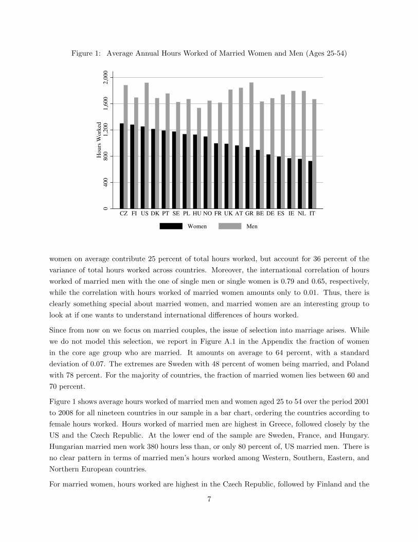
Figure 1: Average Annual Hours Worked of Married Women and Men (Ages 25-54)

0400

800

1,2

00

1,6

00

2,0

00

Hours

Work

ed

CZ FI US DK PT SE PL HU NO FR UK AT GR BE DE ES IE NL IT

Women Men

women on average contribute 25 percent of total hours worked, but account for 36 percent of the

variance of total hours worked across countries. Moreover, the international correlation of hours

worked of married men with the one of single men or single women is 0.79 and 0.65, respectively,

while the correlation with hours worked of married women amounts only to 0.01. Thus, there is

clearly something special about married women, and married women are an interesting group to

look at if one wants to understand international differences of hours worked.

Since from now on we focus on married couples, the issue of selection into marriage arises. While

we do not model this selection, we report in Figure A.1 in the Appendix the fraction of women

in the core age group who are married. It amounts on average to 64 percent, with a standard

deviation of 0.07. The extremes are Sweden with 48 percent of women being married, and Poland

with 78 percent. For the majority of countries, the fraction of married women lies between 60 and

70 percent.

Figure 1 shows average hours worked of married men and women aged 25 to 54 over the period 2001

to 2008 for all nineteen countries in our sample in a bar chart, ordering the countries according to

female hours worked. Hours worked of married men are highest in Greece, followed closely by the

US and the Czech Republic. At the lower end of the sample are Sweden, France, and Hungary.

Hungarian married men work 380 hours less than, or only 80 percent of, US married men. There is

no clear pattern in terms of married men’s hours worked among Western, Southern, Eastern, and

Northern European countries.

For married women, hours worked are highest in the Czech Republic, followed by Finland and the

7

US, while at the lower end are Spain, Ireland, the Netherlands, and Italy. Northern and Eastern

European countries all feature relatively high working hours, while Western European and Southern

European countries are mostly located in the lower half of the sample, the exception being Portugal.

The differences in hours worked of married women are much larger than for married men. Italian

married women, i.e. women in the country exhibiting the lowest hours, work 530 hours less than,

or only 58 percent of, US married women.

4 Model

4.1 A Simple Model of Labor Supply

We build a simple static model featuring a representative married couple whose members jointly

maximize the utility of the household by determining male and female labor supply.18 The house-

hold faces two types of taxes, namely a consumption tax and a non-linear labor income tax. The

government balances the budget by redistributing the taxes in the form of lump-sum transfers,

which the household takes as exogenous.

The household maximizes

maxhm,hf

ln c− αmh

1+ 1φm

m

1 + 1φm

− αfh

1+ 1φf

f

1 + 1φf

(1)

subject to

c =1

(1 + τc)[wmhm + wfhf − τl(wmhm, wfhf , k)] + T (2)

where c represents household consumption, {wg, hg} wages and hours by the husband (g = m) and

the wife (g = f), and k the number of children. τc is the proportional consumption tax, τl the labor

income taxes as a non-linear function of the husband’s and wife’s labor incomes and the number of

children, and T is the lump-sum transfer by the government.

The utility function is inspired by the one used by Guner et al. (2012b).19 As in there and usual in

the literature explaining aggregate hours differences between Europe and the US - even with agents

with heterogenous education choices as in Guvenen et al. (2011) -, consumption and labor supply

18This is similar to Kaygusuz (2010) who however allows for income heterogeneity. Prescott (2004) and Ohanianet al. (2008) obtain their hours predictions from the static first-order condition of the standard neo-classical growthmodel, taking the consumption-output ratio as the forward-looking component directly from the data. McDaniel(2011) solves also the intertemporal first-order condition.

19As in Heathcote et al. (2010) and Jones et al. (2003), we do not explicitly model an extensive margin. We abstractfrom fixed cost of working given the lack of heterogeneity and allow for gender-specific preference heterogeneity,whereas Guner et al. (2012b) impose on women with small children a fixed time cost which increases their marginaldisutility of work.

8

are assumed to be separable, and utility from consumption is logarithmic. α captures the relative

weight on the disutility of work, and φ determines the curvature of this disutility. Both parameters

are gender-specific and thus potentially differ for men and for women. Preference differences by

gender can capture effects like differential impact of children on the labor supply of men and

women.20,21

4.2 Model Inputs

As inputs into the model, we need country-specific information on male hourly wages, female hourly

wages, non-linear labor income taxes, and consumption taxes. Last, we calibrate the four preference

parameters in the utility function. When used in the model, wages and taxes are converted into

2005 US-Dollars, using PPP-adjusted exchange rates.

4.2.1 Hourly Wages

To calculate hourly wages, we have to divide earnings by hours. Unfortunately, the ELFS does not

provide earnings data, and the German Microcensus only net data. Therefore, for the European

countries we use average gross full-time earnings by gender provided by Eurostat (see Appendix

A.3 for a detailed description).22 For the US, we calculate the equivalent statistic from the CPS.

Specifically, we define full-time workers as usually working 35 hours or more. We then take weekly

earnings from the CPS for this group and multiply by 52.23 Last, we divide the gross full-time

earnings by full-time hours by gender. To construct full-time hours by gender, we focus again on

individuals reporting usual hours of 35 or more in the main job, and then multiply usual hours

worked in the main job by 52 minus weeks of vacation and public holidays, before averaging over all

individuals.24 In a robustness check in Section 8, we show that our results are robust to alternative

data on earnings coming from the OECD.

Olivetti and Petrongolo (2008) analyze the effect of self-selection into employment on estimated

gender wage gaps. Full-time working women are a positively self-selected group to a larger extent

than full-time working men, leading to a potential underestimation of the gender wage gap. This

20With the gender wage gap alone, we cannot explain the hours worked difference of 670 hours between marriedmen and women in the US, our baseline country.

21We solve the model numerically, allowing men to choose from an hours grid ranging from 0 to 3000 annual hours,with a step size of 10 hours for the range from 1200 to 2200 hours. The grid for female hours worked also ranges from0 to 3000 hours, with a step size of 10 hours between 500 and 1500 hours. Outside these ranges, step sizes amountto 50 hours.

22Eurostat does not provide any data for Italy and Norway. For Italy, we use the Structure of Earnings Survey(Struttura delle retribuzioni), and for Norway data from Statistics Norway.

23Weekly earnings are capped at 2884 nominal US Dollar in the CPS, potentially leading to an underestimation ofthe true average full-time earnings for the US. However, only 2.3% of male and 0.07% of female weekly earnings arecapped.

24Full-time earnings refer to the main job, and thus we take hours in the main job accordingly. Actual hours workedin the main job are not available for the US, and for consistency purposes we thus work with usual hours worked inthe main job for the calculation of the hourly wages.

9

positive self-selection effect is weaker in countries where a large part of the women work full-time,

additionally introducing cross-country variation in this bias. We apply a country-specific correction

parameter, taken as the simple average over the different estimated ones in Olivetti and Petrongolo

(2008), to the female wages in order to correct for this bias.25

4.2.2 Non-Linear Labor Income Taxes and Consumption Taxes

The non-linear labor income tax system is captured by the OECD Taxing Wages tax modules.

The OECD tax codes calculate annual household net income based on the respective country’s and

year’s tax laws, taking income taxes plus employees’ social security contributions, as well as cash

benefits into account. Tax modules are available online from the year 2001 on. Using these codes,

we can assign an annual net household income to each combination of male and female annual

earnings. We calculate the exact values for an earnings grid with 101 steps for men, ranging from

0 earnings to four times the average annual earnings in the country, and for an earnings grid with

201 steps for women, ranging from 0 earnings to three times the average annual earnings in the

country.26 We then linearly interpolate in two dimensions to assign a net annual household income

to each possible annual hours choice of husband and wife. One additional input into the tax codes

are the number of children. From the micro data, we calculate the percentage of married couples

with 0, 1, 2, 3, or 4+ children,27 and use these to construct a weighted average of net incomes.

For consumption taxes, we use data on value added taxes, averaging for the US across states. In

a robustness check in Section 8, we use the consumption taxes provided by McDaniel (2012), who

calculates consumption tax rates from NIPA data, and results are robust. Comparing these data

to value added taxes, the largest deviations arise for Sweden and Denmark, where excise taxes play

a relatively large role.28

Table 2 summarizes the model inputs. We group the countries according to geographic location

into Scandinavian countries, and Western, Southern, and Eastern European countries. Clearly, it is

impossible to summarize the complex labor income tax systems in a few numbers. Columns 1 and

2 show two possible measures that reflect two aspects of the labor income tax schedule: column

1 (τl(0)) shows the country-specific average tax rate evaluated at the country-specific mean male

25The smallest adjustment is made in the Scandinavian countries and the US (0.97 to 0.99) and the largest in theSouthern European countries and France (0.93 to 0.95). Olivetti and Petrongolo (2008) calculate the adjustmentfactor based on data from 1994 to 2001. They do not analyze Norway, Sweden, and the Eastern European countries.Therefore, we set the adjustment factor to 1 for these countries. Given the relatively high participation of women inthe labor market in these countries, the bias should indeed not be large.

26For women, we thus put in as many steps as the OECD taxing wages module allows. To give a specific example,for the US for the year 2005 the difference between two annual earning levels for men amounts to 2297 US-Dollarsand for women to 689 US-Dollars.

27For Denmark, we use these percentages from the year 1992, and for Norway from 1995, the latest survey yearsrespectively containing information on children. Sweden provides no information on children at all. We therefore usethe Finnish data on children, which is available from 2003 on, also for Sweden.

28For Sweden, consumption taxes are 8.1 percentage points higher than the VAT rate, and for Denmark 6.9percentage points.

10

Table 2: Model Inputs

Country τl(0) τ ′l (h

USf ) τc wm

wf

wm

Denmark 37.4 47.9 25.0 24.5 84.8

Finland 33.3 26.7 22.0 18.0 83.5

Norway 26.0 29.6 24.4 23.7 90.0

Sweden 31.0 28.7 25.0 20.1 84.2

Mean 31.9 33.3 24.1 21.6 85.6

Austria 32.7 22.7 20.0 24.2 65.9

Belgium 31.0 47.9 21.0 22.3 84.9

France 22.4 32.3 19.6 18.2 81.0

Ireland 13.6 18.1 21.0 19.8 76.9

Germany 31.3 49.6 16.4 25.3 76.7

Netherlands 28.6 33.9 19.0 24.2 74.9

United Kingdom 25.9 19.5 17.5 24.8 74.7

Mean 26.5 32.0 19.2 22.7 76.4

Czech Republic 21.5 23.2 20.7 8.1 75.8

Hungary 32.3 24.4 23.6 7.8 83.8

Poland 28.6 32.5 22.0 7.8 88.3

Mean 27.5 26.7 22.1 7.9 82.6

Spain 15.6 18.9 16.0 15.3 77.1

Greece 20.9 16.0 18.3 12.8 73.7

Italy 25.6 28.7 20.0 18.1 87.4

Portugal 17.4 21.3 19.0 11.2 73.1

Mean 19.9 21.2 18.3 14.4 77.8

United States 21.1 29.1 4.8 21.7 80.7

Note: τl(0) is the country-specific average tax rate evaluated at the average country-specific annual hours worked by married men, assuming the wife does not work.τl′(hUSf ) is the average marginal tax rate if the wife starts working and works theaverage hours of US married women, i.e. [τl(wmhm, wfh

USf ) − τl(wmhm, 0)]/[wfh

USf ].

Both tax rates are calculated for couples without children. Male hourly wages (wm)are given in 2005 real, PPP adjusted US Dollars.

annual income (wCmhCm), assuming that the woman does not work, and thus gives one of many

possible measures of an average tax rate. Column 2 (τl′(hUSf )) shows the average marginal tax rate

if the woman starts working and works the mean hours of US married women, thereby capturing one

possible measure of progressivity.29 The US average tax rate as calculated in column 1 amounts to

29We define this average marginal tax rate as [τl(wmhm, wfhUSf ) − τl(wmhm, 0)]/[wfh

USf ]. Both tax rates are

calculated for couples without children, as the latter decrease τl(0) via tax credits etc., but hardly affect τl′(hUSf ).

11

19.9%, whereas the corresponding Danish married couple would have to pay an average tax rate of

37.4%, and the Irish couple a tax rate of only 13.6%. The average tax rates are lowest in Southern

Europe and the US, followed by Western and Eastern Europe, and highest in Scandinavia. The

measure of progressivity shown in column 2 amounts to 29.1% in the US, peaking at 49.6% in

Germany, a country with high progressivity and joint taxation of married couples. This measure is

again on average lowest in Southern Europe, followed by Eastern Europe and the US, and highest

in Scandinavia and Western Europe. The differences in the consumption taxes between the US and

Europe are large, in particular for the Scandinavian countries. Male hourly wages are on average

similar in the US, Scandinavia, and Western Europe, but smaller in Southern Europe and smallest

in Eastern Europe. The gender wage gap is least favorable for women in Western Europe, followed

by Southern Europe, the US, and Eastern Europe, with the lowest gender wage gap in Scandinavia.

4.2.3 Calibration of Preference Parameters

The four preference parameters to be calibrated in the model are the parameters αm, αf , φm and

φf , which refer to the relative weight on the disutility of work and its curvature, separately for

men and women. We calibrate these parameters to match average hours worked in the US over

the time period 2001 to 2008 for both married men and women, as well as an uncompensated wage

elasticity of 0.79 for women, which is the median value for women given in the survey article by

Blundell and MaCurdy (1999), and an uncompensated wage elasticity of 0.2 for men.30 With these

targets, we calibrate αm = 1.77, αf = 1.03, φm = 0.48, and φf = 1.43. The calibrated curvature

parameter on the disutility of work is much higher for women than for men.31 On the other hand,

the implied disutility weight on hours worked

(α

1+ 1φ

)is similar for both men (0.57) and women

(0.61). We match all four targets almost perfectly.32

4.3 Time-Series Performance of the Model

While the goal of the paper is to use the model to evaluate in how far differences in taxes and

wages can explain cross-country differences in hours worked of married women (and men), we can

evaluate the predictive power of the model also by analyzing its performance in replicating the US

time series of hours worked of married couples. To do that, we generate the US-specific model

30Typical estimates of the uncompensated wage elasticity for men range around negative values to 0.2, so our valueis on the upper side of the estimates. However, both Keane (2011) and Chetty (2012) argue that these estimateslikely underestimate the true elasticity, due to optimization frictions and the failure of most studies to account forreturns to work experience. In Section 8, we show a robustness check in which we target a male elasticity of 0.1.The cross-country fit of hours worked of married men deteriorates somewhat, but the fit for married women remainsalmost unchanged.

31Note that in a dynamic context, the parameter φ would correspond to the Frisch elasticity, and the value formen falls in the typically estimated range. This interpretation has to be taken with caution as we are explicitly nottargeting the Frisch elasticity, but an uncompensated wage elasticity, given the static setup of our model.

32Male hours worked in the model are 1252, compared to 1251 in the data, female hours 1917 compared to 1918,and the elasticity in the model is 0.192 and 0.785 for men and women, respectively.

12

Figure 2: Time-Series Predictions for the US

800

1000

1200

1400

1600

1800

2000

Annual

Hours

1980 1985 1990 1995 2000 2005 2010

Year

Men Data Model

Women Data Model

inputs back to the year 1979 and plug them into the model, keeping the preference parameter

values fixed.33 As Figure 2 shows, the model correctly predicts hardly any change in hours worked

of married men over the period of three decades. For married women, the model accounts for 2/3 of

the increase in hours worked between 1979 and 2008, indicating that women worked 18 percent less

in the late 70s/early 80s than in the 2000s, while in fact they worked 27 percent less. The increase

in the 1980s, when several tax reforms favored married women (see Kaygusuz (2010)), is captured

correctly by the model, but the model underpredicts the increase in hours worked in the 1990s.

This is in line with estimates by Guner et al. (2012a), who show that average tax functions in

the US changed dramatically between 1980 and 1989, but remained almost constant between 1989

and 2000. Moreover, the wage gap decreased significantly until 1993, but only slightly afterwards.

In Section 5.2, we compare the time series prediction of our model to a model with linear taxes,

underlining the importance of the modeling of non-linearities in the taxation of married couples.

Overall, our model performs quite well in explaining the US time series of hours worked.

5 Results

Keeping the preference parameters fixed across countries, we use country-specific inputs of taxes

and wages in order to obtain predicted hours worked of married couples across countries. We

33For the labor income taxes in the US, we can use the NBER TaxSim module, which goes back to the 70s. As inthe OECD TaxBen module we use the state tax of Michigan and the city tax of Detroit.

13

first present the cross-sectional predictions of hours worked of married men, before we move to

the core result of hours worked of married women. Using the US as the benchmark country, we

always compare deviations from US hours in model and data. Next, we compare our results to

predictions from a model with linear taxes, as e.g. in Ohanian et al. (2008) and McDaniel (2011).

In a decomposition analysis, we evaluate the relative importance of wages and taxes in explaining

the cross-country variations of married women’s hours worked. Last, we further analyze the effects

of labor income taxes by decomposing them into differences in average tax rates and differences in

marginal tax rate schedules.

5.1 Hours Worked in Model and Data

Table 3 shows in the first column the percentage difference in married men’s hours worked between

the respective country and the US in the data, and in the second column the model predicted

percentage difference. Within each geographic group, we order the countries according to the

percentage difference to hours worked in the US.

Differences in taxation and wages explain the cross-country variation in married men’s hours worked

very well. While married men in Scandinavia work 13 percent less than married men in the US in the

data, the model predicts on average a difference of minus 12 percent. For Western Europe, the model

also achieves an almost perfect fit on average, and predicts 8 percent lower hours worked, compared

to 9 percent lower hours in the data. For Southern Europe, the model slightly underpredicts the

difference in hours worked to the US, while for Eastern Europe the model on average achieves a

perfect fit. Focusing on individual countries, for 14 countries the differences between prediction

and data amount to 5 percentage points or less, and for 9 countries even to 3 percentage points or

less. France is the country with the largest difference between model and data, amounting to 12

percentage points.

We now turn to our main results of interest, namely predicted hours worked of married women, in

Table 4. Scandinavian married women work on average 5 percent less than US ones in the data,

while the model, based on the differences in taxes and wages only, generates a difference of minus 16

percent. This overprediction of the difference is mostly driven by Denmark and Finland, where the

model generates a difference of minus 25 and minus 12 percent respectively, but the true differences

are only minus 3 and plus 3 percent. Sweden and in particular Norway are predicted fairly well.

Ragan (2012), Rogerson (2007) and Olovsson (2009) show that modelling home production helps

in generating the high average hours worked of the entire population in Scandinavia. Two further

features are particularly important here: first, many transfers rely on the working status of the

individual, rather than being simple lump-sum transfer, and secondly, many transfers come in the

form of subsidized goods in the service sector (especially subsidized child care). Adding these

extensions to the basic model would give additional incentives for the individual to work and

enjoy these transfers. Indeed, adding child care costs to the model as done in Section 6 increases

14

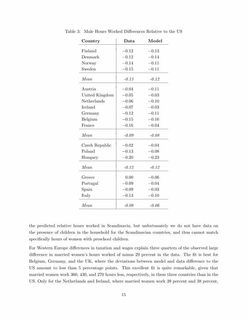
Table 3: Male Hours Worked Differences Relative to the US

Country Data Model

Finland −0.12 −0.13

Denmark −0.12 −0.14

Norway −0.14 −0.11

Sweden −0.15 −0.11

Mean -0.13 -0.12

Austria −0.04 −0.11

United Kingdom −0.05 −0.03

Netherlands −0.06 −0.10

Ireland −0.07 −0.03

Germany −0.12 −0.11

Belgium −0.15 −0.16

France −0.16 −0.04

Mean -0.09 -0.08

Czech Republic −0.02 −0.04

Poland −0.13 −0.08

Hungary −0.20 −0.23

Mean -0.12 -0.12

Greece 0.00 −0.06

Portugal −0.09 −0.04

Spain −0.09 −0.03

Italy −0.13 −0.10

Mean -0.08 -0.06

the predicted relative hours worked in Scandinavia, but unfortunately we do not have data on

the presence of children in the household for the Scandinavian countries, and thus cannot match

specifically hours of women with preschool children.

For Western Europe differences in taxation and wages explain three quarters of the observed large

difference in married women’s hours worked of minus 29 percent in the data. The fit is best for

Belgium, Germany, and the UK, where the deviations between model and data difference to the

US amount to less than 5 percentage points. This excellent fit is quite remarkable, given that

married women work 360, 430, and 270 hours less, respectively, in these three countries than in the

US. Only for the Netherlands and Ireland, where married women work 39 percent and 38 percent,

15

Table 4: Female Hours Worked Differences Relative to the US

Country Data Model

Finland 0.03 −0.12

Denmark −0.03 −0.25

Sweden −0.06 −0.15

Norway −0.12 −0.11

Mean -0.05 -0.16

France −0.20 −0.12

United Kingdom −0.21 −0.18

Austria −0.23 −0.15

Belgium −0.28 −0.31

Germany −0.34 −0.35

Ireland −0.38 −0.16

Netherlands −0.39 −0.19

Mean -0.29 -0.21

Czech Republic 0.04 −0.15

Poland −0.09 −0.10

Hungary −0.10 −0.10

Mean -0.05 -0.12

Portugal −0.05 −0.23

Greece −0.25 0.03

Spain −0.37 −0.04

Italy −0.42 −0.12

Mean -0.27 -0.09

respectively, less than in the US, can the model explain only half of the difference.

For Eastern Europe, differences in taxes and wages generate too low hours relative to the US, i.e.

differences are overpredicted. This is however entirely driven by the Czech Republic: for Poland

and Hungary, the model generates a perfect fit in predicted hours worked differences.

Differences in taxes and wages cannot explain married women’s hours worked for Southern European

countries as compared to the US. Portuguese married women work only 5 percent less hours than

US ones, while the model predicts minus 23 percent. For Greece and Spain the difficulty goes in the

opposite direction: in the data, married women work 25 and 37 percent less than in the US, while

the model predicts a difference of plus 3 percent, or only minus 4, respectively. Thus, there are

16

clearly some effects at work in Southern Europe which go beyond taxes and wages. The predictive

power for Italy is lower than for Western Europe, but still amounts to 30 percent. Chakraborty

et al. (2012) attribute the low female hours worked in Southern Europe to the low divorce risk;

in addition, there might be other cultural factors at play that are correlated with divorce risk.

Moreover, in all Southern European countries part-time work plays a relatively minor role in the

data. If the decision of how much to work is restricted to being basically a decision between

working full-time or not to work at all, it could be that relatively small differences in incentives

lead to relatively large differences in outcomes, as e.g. observed between Portugal, where married

women work almost 1200 hours, and Spain, where they work less than 800 hours.34

Thus, we conclude that differences in taxes and wages are able to explain three quarters of the

large hours worked differences between Western Europe and the US. For Scandinavia and Eastern

Europe, differences in taxes and wages overpredict hours worked differences relative to the US, but

still generate a decent fit. For Southern Europe, however, differences in taxes and wages cannot

explain the observed low hours worked in Spain, Greece, and Italy, and the high hours worked in

Portugal.

5.2 Actual Taxes vs. Linear Taxes

One major novelty of our study is that we use actual tax systems as model inputs. To understand

how important this is, we compare our results to results from a model where simple linear taxes

are used as inputs. Specifically, we use the linear tax rates calculated by Ohanian et al. (2008).35

We recalibrate the model in order to still match the four moments. For simplicity, we report from

now onwards directly the hours worked differences of married women for the four country groups

and provide the detailed tables with all countries in the Appendix.36

As Table 5 shows, the predicted hours worked are on average lower in the model with linear taxes

than in the model that uses actual taxes as input. This worsens the fit for Scandinavia and Eastern

Europe, but somewhat improves the fit for Southern Europe. For Western Europe, the average

fit is somewhat better with linear taxes, but this result holds only on average; as Table A.1 in

the Appendix shows, the mean absolute deviation between model and data is exactly the same for

Western Europe under both models. Thus, overall the model with actual taxes performs better

than the model with linear taxes.

The lower hours worked in the model with linear taxes than in the model with actual taxes are

34The difference between married women’s hours worked in Portugal and Spain cannot be explained by differencesin divorce risk in the model by Chakraborty et al. (2012).

35Prescott (2004) and McDaniel (2011) multiply these average tax rates by a factor of 1.6 in order to convert theminto average marginal tax rates.

36Table A.1 in the Appendix shows the results with linear taxes for each country for women, and Table A.2 formen. For married men, our model predicts hours worked slightly better than the model with linear taxes, but thedifferences are relatively small. This shows that for married men average tax rates seem to be a decent approximationof actual tax rates.

17

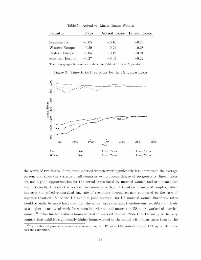
Table 5: Actual vs. Linear Taxes: Women

Country Data Actual Taxes Linear Taxes

Scandinavia −0.05 −0.16 −0.23

Western Europe −0.29 −0.21 −0.28

Eastern Europe −0.05 −0.12 −0.21

Southern Europe −0.27 −0.09 −0.22

The country-specific results are shown in Table A.1 in the Appendix.

Figure 3: Time-Series Predictions for the US: Linear Taxes

800

1000

1200

1400

1600

1800

2000

Annual

Hours

1980 1985 1990 1995 2000 2005 2010

Year

Men Data Actual Taxes Linear Taxes

Women Data Actual Taxes Linear Taxes

the result of two forces. First, since married women work significantly less hours than the average

person, and since tax systems in all countries exhibit some degree of progressivity, linear taxes

are not a good approximation for the actual taxes faced by married women and are in fact too

high. Secondly, this effect is reversed in countries with joint taxation of married couples, which

increases the effective marginal tax rate of secondary income earners compared to the case of

separate taxation. Since the US exhibits joint taxation, for US married women linear tax rates

would actually be more favorable than the actual tax rates, and therefore our re-calibration leads

to a higher disutility of work for women in order to still match the US hours worked of married

women.37 This further reduces hours worked of married women. Note that Germany is the only

country that exhibits significantly higher hours worked in the model with linear taxes than in the

37The calibrated parameter values for women are αf = 1.12, φf = 1.52, instead of αf = 1.03, φf = 1.43 in thebaseline calibration.

18

Table 6: Decomposing Female Hours Worked Differences Relative to the US

Country Data Model τl τc τl + τcwf

ym

Scandinavia −0.05 −0.15 −0.14 −0.15 −0.26 0.12

Western Europe −0.29 −0.19 −0.15 −0.12 −0.22 0.03

Eastern Europe −0.05 −0.12 −0.08 −0.14 −0.19 0.09

Southern Europe −0.27 −0.10 0.00 −0.11 −0.11 0.03

Note: Male hours are fixed at country-specific means. For the decomposition (columns 3 to 6) one model input is setcountry-specific at once and the rest are left unchanged at their US values. The country-specific results are shownin Table A.3 in the Appendix.

model with actual taxes; this is the country that combines joint taxation with a high degree of

progressivity.

We also compare the US time-series prediction of the model with actual taxes to the one of the

model with linear taxes in Figure 3. As one can see, the model with linear taxes only accounts for

one third of the increase in hours worked of married women since the late 1970s, and specifically

does not capture the effects of the tax reforms in the 1980s that increased incentives to work for

married women. Overall, we conclude that if one wants to explain hours worked of married women,

it is important to take the non-linearities of the tax schedule into account.

5.3 Decomposition Analysis

To understand the relative importance of wages and taxes in explaining the cross-country differ-

ences, we simulate the model setting only one input factor country-specific and leaving all other

input factors at the respective US level.38 We fix male hours worked exogenously at the respective

empirically observed country-specific level in this decomposition analysis and denote the implied

male income with yCm. This makes the interpretation of the decomposition results for women more

straightforward.39 The second column in Table 6 shows the predicted percentage difference be-

tween married women’s hours worked in the respective country group and the US for the model

with exogenous male labor supply when all four factors are set country-specific. The results are

very similar to the ones presented in Table 4, since male hours worked are very well predicted by

the model.

The third column in Table 6 presents predicted hours worked if only the labor income tax system

is set country-specific. In order to avoid that due to different income levels in the US and the

respective country one ends up in different progressivity ranges if applying the country specific tax

38Transfers are adjusted in these decomposition analyses such that the government always maintains a balancedbudget.

39The utility function then simplifies to u(c, hf ) = ln c− αfh1+ 1

φff

1+ 1φf

.

19

code but maintaining US income levels, we proceed as follows: we calculate the tax rate for all

possible country specific income levels given the female hours grid, and apply this tax rate to the US

gross income given the same female hours worked, i.e. for all possible female hours hf , we calculate

the taxes as TAX(hf ) =(yusm + wUSf hf

)τCl (yCm,wCf hf)yCm+wCf hf

. As the Table shows, the disincentive effects

of the country-specific labor income tax systems relative to the US one are largest in Western

Europe, closely followed by Scandinavia. In both country groups, labor income taxes alone predict

15 or 14 percent lower hours worked of married women than in the US, respectively. For Eastern

Europe, the effect is half the size, and it is absent on average in Southern Europe. Concluding, one

can say that despite the joint taxation of married couples in the US, the labor income tax system

in the US is relatively favorable for secondary income earners due to the relatively low average tax

rates and the relatively mild level of progressivity.

The next column shows predicted hours worked differences relative to the US if only consumption

taxes are set country-specific. Not surprisingly, the effects are largest for Scandinavia, where

consumption taxes are highest. Here, consumption taxes alone would predict that Scandinavian

married women should work 15 percent less than US ones. For all other European regions, the

effects of consumption taxes alone on married women’s labor supply are also sizeable, ranging

between predicting 11 to 14 percent lower hours worked than in the US. Column 5 shows the joint

effect of taxation, setting both labor and consumption taxes country-specific. The joint effect of

taxation is smaller than the sum of the individual effects of both taxes, pointing to important

interaction effects. Both taxes together predict between 19 and 26 percent lower hours worked of

married women in Europe than in the US, with the exception of Southern Europe, where the effect

of taxes is smaller and only adds up to 11 percent, due to the absence of any effect of labor taxation.

The last column presents the effects if the female wage to male income ratio is set country-specific,

while the male incomes are left at the US level. This statistic is somewhat different from the gender

wage gap, since male earnings vary with both male hourly wages and male hours worked. We again

adjust taxes to keep tax rates for the same hours choices constant.40 As the Table shows, for all

regions predicted hours worked are higher than in the US if the female wage to male income ratios

are set country-specific, reflecting the low female wage to male income ratio in the US. The effect is

small for the Western and Southern European countries, where female wage to male income ratios

are similar to the ones in the US, but sizeable for Eastern Europe and Scandinavia, where predicted

hours worked of married women are 9 and 12 percent higher than in the US, respectively, if the

female wage to male income ratio is set country-specific.

Summarizing, the decomposition analysis shows that differences in taxes are of great importance in

explaining the lower hours worked of married women in Europe than in the US. The higher female

wage to male income ratio in Europe counteracts the effects of taxation and generates higher hours

40Specifically, the wage w inserted in the model satisfieswfyUSm

=wCfyCm

and the taxes amount to TAX(hf ) =(yUSm + wfhf

) τUSl (yUSm ,wUSf hf )yUSm +wUS

fhf

.

20

worked of married women in Europe than in the US. For Southern and Eastern Europe, differences

in consumption taxes are more important than differences in labor income taxes in explaining hours

worked differences to the US, while for Western Europe the opposite is true. For Scandinavia, both

taxes have disincentive effects of similar magnitudes.

5.4 The Role of Non-Linear Labor Income Taxes

There are two components of the labor income tax code which can potentially differ between the US

and other countries, namely the average tax rate, i.e. the level of the tax schedule, and the actual

marginal tax schedule, which defines how marginal tax rates change with income, and reflects

among other things the progressivity of the tax system.41 Table 5 already gave some indication

that average country tax rates, built by taking averages over the entire population, do not capture

tax disincentives of married women well. In this subsection, we further decompose the actual tax

schedule into the average tax rate for married women and the marginal tax schedule.

To implement the concept of “maintaining the marginal tax schedule”, we keep differences in

marginal tax rates for different income levels constant, and shift the entire marginal tax rate

schedule up or down by levying an additional proportional tax rate (or subsidy) θ on the gross

earnings, such that the budget constraint becomes

c =1

(1 + τc)[ym + wfhf − τl(ym, wfhf )− θ ∗ (ym + wfhf )] + T. (3)

We add θ to the country-specific tax codes in order to achieve the same average tax rate as in

the US, while maintaining the country-specific tax structure.42 The effect of the country-specific

average tax rate is then indirectly inferred by the difference in hours worked between setting the

entire labor income tax schedule country specific, or shifting it up or down to match the US average

tax rate.

Table 7 shows the resulting decomposition of the labor income tax effect into the tax structure and

the average tax rate. The average tax rate has the largest disincentive effect in Scandinavia, followed

by Eastern and Western Europe. When it comes to the tax structure, only Western European

tax codes provide significant disincentive effects compared to the United States, a country with

joint taxation of married couples. This is mostly driven by Belgium, Germany, Ireland, and the

Netherlands. For the Western European countries, differences in the tax structure are on average

more important than differences in the average tax rates, while for Scandinavia and Eastern Europe

41Note that the actual marginal tax schedules, taking exemptions, caps on taxable income for social securitycontributions, etc., into account, often exhibit income ranges where marginal tax rates are falling instead of rising,such that a standard definition of progressivity, namely that marginal tax rates are rising with income, does not applyover the entire income range.

42We do not use the opposite approach, namely adjusting the US tax schedule to match the country-specific averagetax rates, since we do not match hours in all countries well, resulting in imprecise estimates of the country-specificaverage tax rate.

21

Table 7: The Effect of Tax Structure and Average Tax Rates on Female Hours Worked DifferencesRelative to the US

Country Data τl Tax Structure Average Tax Rate

Scandinavia −0.05 −0.14 −0.03 −0.11

Western Europe −0.29 −0.15 −0.13 −0.02

Eastern Europe −0.05 −0.08 −0.02 −0.06

Southern Europe −0.27 0.00 −0.01 0.01

Note: Male hours are fixed at country-specific means. Columns 3 and 4 add up to Column2. Column 2 corresponds to column 3 in Table 6. The country-specific results are shown inTable A.4 in the Appendix.

it is the other way round. For Southern Europe, both effects are small and offset each other. We

conclude that both average tax rates and tax structures are important to explain hours worked

differences of married women between Europe and the US, with the latter mainly mattering for

Western Europe.43

6 The Role of Children

One natural factor that could potentially explain hours worked differences between married women

and the rest of the population is the more likely presence of children. Indeed, in the US mar-

ried women with preschool children (aged 0 to 4) work 950 hours, while married women without

preschool children work 1360 hours, i.e. more than 400 hours more. Different fertility rates, child

care costs, and maternity policies could thus also affect the international differences of hours worked

of married women.

In this section, we analyze hours worked of married women with and without preschool children

separately. We define preschool children as being aged 0 to 4, since this is the available age category

in the ELFS. Unfortunately, for the Scandinavian countries we have no information on children in

the ELFS, and thus we have to omit them from this analysis.44 For women with preschool children,

we add the predicted effects of child care cost and availability on hours worked. From the OECD,

we have information on the cost of full-time day care slots for all countries but Italy (see Appendix

A.4 for a description of these data). We convert these costs into hourly costs by assuming that a

full-time slot covers 40 hours weekly. We call these “minimum child care costs”, since these costs

43As an alternative to adding a linear tax in order to shift the average tax rate, we follow Guvenen et al. (2011),

who require that for any gross income level z the following condition has to be satisfied:1−τ ′l (z)1−τ ′

l(z)

= (1− κ)∀z, where

τ ′l is the marginal tax rate of the original tax schedule, τ ′l is the marginal tax rate of the schedule allowing for adifferent average tax rate, and κ is a constant. Results using this approach are quantitatively similar and are shownin the Appendix in Table A.5.

44Yet, using child care cost related input factors, the model would predict smaller differences of hours workedbetween Scandinavia and the US than the ones in the baseline results, potentially increasing the fit of the model.

22

refer to child care in formal child care centers, which are often subsidized in Europe.

Many European countries not only subsidize their formal child care centers, but ration them sub-

stantially, such that supply might not meet demand at the given price. Unfortunately, we do not

have information on the availability of child care slots. Therefore, we use the enrollment rates in

formal child care as a lower bound for the supply of child care slots at the given price.45 We then

assume that child care beyond this supply has to be purchased in the free market. In the absence of

data on the cost of child care on the free market, we take the third decile of female hourly wages as

an approximation of this cost.46 The total hourly child care costs are then calculated as an average

of the cost for a slot in formal child care center and the cost on the free market, weighted by the

country-specific enrollment rate. We call these costs “maximum child care costs”. The more the

enrollment rate reflects the rationed supply of child care, the closer are the true child care costs

to the “maximum child care costs”; the less this is the case, the closer they are to the “minimum

child care costs”.

As is commonly done in the literature (see e.g. Domeij and Klein, 2012), we assume that for each

hour worked and each child, the woman has to buy one hour of child care. The number of children

in preschool age conditional on having at least one child in this age group is taken directly from

the data.47 We calibrate the model separately for women with and without preschool children,

each time matching the respective hours worked in the US (950 and 1360, respectively), and an

uncompensated wage elasticity of 0.79.48 For women with preschool children, we calibrate the

model separately assuming no, minimum, or maximum child care costs. When simulating country

specific hours worked for women with preschool children, we set not only the four usual input

factors country specific, but also child care costs and the number of preschool children per woman.

Table 8 shows the hours worked differences of married women without preschool children relative

to the US. The fit is almost unchanged when compared to the fit for all married women. More

interesting are the results for women with preschool children. Table A.6 in the Appendix shows the

additional country-specific inputs into the model: the average number of preschool children is lower

in all European regions than in the US. Minimum child care costs relative to the female wage are

lowest in Eastern Europe and Scandinavia, followed by Southern Europe and the US. Going from

minimum to maximum child care costs, they remain highest in Western Europe. Table 9 shows

the model results. For Western Europe, hours worked are matched very well assuming maximum

child care costs. For Eastern Europe, we underpredict the difference to the US even with maximum

45Enrollment rates are provided by the OECD. We take weighted averages of the enrollment rates of children aged0 to 2 and 3 to 5 to get the enrollment rates of children aged 0 to 4. For most countries, we also have separateinformation of the costs of slots for children aged 0 to 2 and children aged 3 to 5, and similarly take the weightedaverage.

46These data are available from the OECD, as described in Appendix A.5.47The NBER MORG data only contain information on whether preschool children are present. We therefore obtain

the number of children in preschool age conditional on having at least one child in this age group from the MarchCPS using the same sample selection criteria.

48For simplicity, we set male hours worked exogenously at the country-specific level of married men with or withoutpreschool children, respectively. For men, hours do not vary much with the presence of children within a given country.

23

Table 8: Hours Worked Differences of Married Women Without Preschool Children Relative tothe US

Country Data Model

Western Europe −0.29 −0.23

Southern Europe −0.31 −0.10

Eastern Europe −0.02 −0.13

Note: Male hours are fixed at country-specificmeans. The country-specific results are shown inTable A.7 in the Appendix.

Table 9: Hours Worked Differences of Married Women With Preschool Children Relative to theUS

Country Data No ccc Min ccc Max ccc

Western Europe −0.33 −0.15 −0.14 −0.32

Southern Europe −0.04 −0.01 0.07 0.07

Eastern Europe −0.38 −0.16 0.04 −0.19

Note: ccc stands for child care costs. Male hours are fixed at country-specific means.The country-specific results are shown in Table A.8 in the Appendix.

child care costs. Interestingly, for Southern Europe the model generates a better match for women

with preschool children than for women without preschool children. However, this comes from the

fact that in Southern Europe both women with and without children work very similar hours. This

indicates that factors other than children play a role in explaining the low hours worked in Southern

Europe.

In an additional exercise, we also add maternity leave regulations into the model. From the OECD,

we have information on the number of fully paid weeks of maternity leave. Assuming the country

specific hourly female wage and country specific average hours worked, we convert this information

into a lump-sum payment for the household. This payment reduces the incentives of women to

work. Yet, even though the weeks of paid maternity leave can add up to half a year or even a full

year in many European countries, the effect of these payments is quantitatively small, changing

the difference in hours worked of married females with preschool children to the US only by 1 to 2

percentage points for most countries. Intuitively, these payments are small compared to the average

male income, especially since they apply only in one single year, not for every year in which the

woman has a preschool child at home.49

49Numerically, we divide the payment by five to get an annual amount over the 5 year period with preschool children,and then multiply by the average number of preschool children in households with preschool children. Results areavailable upon request.

24

Table 10: Female Hours Worked Differences Relative to the US with Wage Heterogeneity

Country Data Homogeneity Heterogeneity

Scandinavia −0.05 −0.16 −0.08

Western Europe −0.29 −0.21 −0.20

Eastern Europe −0.05 −0.12 −0.06

Southern Europe −0.27 −0.09 −0.03

The country-specific results are shown in Table A.10 in the Appendix.

7 Introducing Heterogeneity

In this section, we introduce wage heterogeneity across households within a country. Unfortunately,

neither the ELFS nor the German Microcensus provide gross wages or earnings, which would allow

us to directly estimate both the wage distribution and the degree of assortative matching. Therefore,

we capture matching behavior of men and women into couples by focusing on the three possible

education states high, medium, and low education. From our micro data, we can directly estimate

the distribution of households into the nine possible household education states combining education

of husband and wife.50

To match a wage to each education state, we assume a log-normal distribution of wages. The

variance of log wages is obtained from fitting a log-normal distribution to country-specific male

full-time wage deciles provided by the OECD.51 Cutting off the highest and lowest deciles of the

estimated wage distribution, we discretize the rest into three states based on the male percentile

distribution into high, medium, and low education in the data, and then calculate the mean wage

within each state.52 Last, we rescale wages such that the overall mean wage corresponds to the

CPS or Eurostat mean male wage in the respective country/year. For female wages, we follow the

same procedure, assuming the same variance as for male wages, but taking the female education

distribution from the data. After doing that, we can assign to each of the nine household education

types female and male wages. We recalibrate the model to match average male and female hours

from the US, as well as the average male and female uncompensated wage elasticities, and again

achieve an almost perfect match.

50For Denmark, we use these percentages from the year 1992, the latest survey year containing information on thespousal educational level. Sweden and Norway provide no information on the spousal educational level at all. Wetherefore use the Finnish data also for Sweden and Norway.

51The OECD provides full-time earnings deciles, which we convert into full-time wages using our data on full-timehours.

52We take the logarithmic wage distribution with the estimated variance, cut off the highest and lowest deciles, anddivide the rest between the 10th and the 90th percentile into the three education groups according to the percentagesin the data. We cut off the extremes in order to be able to estimate a mean wage. E.g. if 20% of the population havehigh or low education, respectively, and 60% medium education, we calculate the mean wage for the 10th to 20thpercentile of the wage distribution and allocate it to the low education group, allocate the mean wage of the 20th tothe 80th percentile to the middle education group, and allocate the mean wage of the 80th to the 90th percentile tothe high education group.

25

As Table 10 shows, introducing wage heterogeneity generally raises female hours worked compared

to the US.53 This improves the model fit for the Scandinavian countries, as well as the Eastern

European countries. In fact, the model can now predict married women’s hours worked in both

regions very well. For Western Europe, the average difference to the US is almost the same assuming

homogeneous or heterogeneous wages. Only for Southern Europe does the model fit worsen even

further. Thus, introducing heterogeneity in wages improves the overall predictive power of taxes

and wages.54

Going from the model with homogenous wages to the one with heterogeneous wages introduces

variation across countries in the wage distribution and in the matching of couples. These differences

interact with differences in the non-linear labor income tax system in a complex way. We try to get

some intuition for the results through decomposition analyses. In one decomposition, we keep the

heterogeneity of the US and simply introduce country-specific tax systems, as done in Section 5.3.

For Scandinavia, the predicted difference in female hours to the US is 6 percentage points smaller

in this exercise under the assumption of heterogeneity than under homogeneity, while for the other

regions the difference amounts only to 1 to 3 percentage points. A further decomposition analysis

keeps the US tax system, but introduces country-specific heterogeneity in wages and matching.

This increases hours worked relative to the US by 4 to 6 percentage points for all four regions.

For Scandinavia, the effect comes more from the heterogeneity itself than from the matching into

couples, while for the other regions both effects are of similar size. Summarizing, our results

indicate that the heterogeneity itself, rather than the tax treatment of heterogeneity, leads to

the lower predicted difference to the US for all four regions. In Scandinavia, the effect is larger

than in the other three regions through an added effect of taxation. Two caveats come with this

interpretation. First, of course these effects interact in complicated ways. Second, our measure

of heterogeneity is unfortunately a rather crude one, and results might be different with a more

complete picture of country-specific heterogeneity.55

7.1 Joint vs. Separate Taxation

In a model with heterogeneity, we can also look closer at the effects of joint vs. separate taxation of

married couples, which can potentially have large effects on female labor supply in heterogeneous

matches. We can get an insight into the degree of individual taxation in the sample countries

by comparing two singles living together in one household with a married couple living in one

household. To avoid further complications, we analyze the case of no children. Both households

share the same utility function, but have different budget constraints, since the members of the first

53Exceptions to this rule are Austria and Germany.54For men, the explanatory power of the model deteriorates slightly when heterogeneity is introduced. Yet, the

average deviation in married men’s hours worked from the US does not change by more than four percentage pointsfor any region, see Table A.9 in the Appendix.

55Our heterogeneity measure is especially crude for countries in which a large part of the population share thesame education status, which is most notably the case in Portugal and Eastern Europe.

26

Figure 4: Current System vs. System of Strictly Separate Filing

−100

−50

050

100

150

200

250

300

Hours

Dif

fere

nce

DE IE PT US FR DK CZ IT BE PL FI SE AT HU UK NO ES GR NL

Women Men

Note: This figure shows the predicted changes in hours worked when going from the current country-specificsystem of filing to a system of strictly separate taxation of married couples, keeping the average householdtax rate constant.

household are taxed as singles, while the members of the second household are taxed as a married

couple. For the household with two singles, the budget constraint becomes

c =1

(1 + τc)[wmhm − τl(wmhm) + wfhf − τl(wfhf )] + T. (4)

The net income in the household with two singles is equal to the sum of the net income of the two

household members, both taxed as singles.

We add a proportional tax/subsidy rate θ as in Section 5.4 when going to separate taxation, such

that the average tax rate of the household with two singles equals the average tax rate of the

married household, both times under optimal hours decision of the woman. Therefore, we do not

capture effects coming from different average tax rates of both households.56

As Figure 4 shows, for around two thirds of the countries there is almost or exactly no difference

between the current tax system and a system of separate taxation at the three possible wage

states which we allow for men and women.57 For Denmark and France, going to a system of

56Studies investigating tax reforms usually require pre- and post-reform tax revenues to remain constant, while werequire the pre- and post-reform average tax rate to be constant. In our context, we prefer the latter, because it isthe relevant number from the household’s perspective.

57It could still be that for very low income earners the systems offer special tax brakes for married couples with asole income earner.

27

strictly separate taxation increases married women’s hours worked by 50 and 70 hours per year,

respectively. There are four countries for which this transition significantly increases hours worked

of married women, namely the US, Portugal, Ireland, and Germany. For the US, Portugal, and

Ireland, three countries with joint taxation of married couples, the quantitative effects amount

to 100, 110, and 150 hours annually, respectively. The country for which a transition to strictly

separate taxation has the largest effect is Germany. Here, hours worked of married women would

increase by 270 hours annually, i.e. by 33 per cent, if a system of separate taxation of married

couples would be introduced. The large effects for Germany arise because the current German

tax code has a system of joint taxation, and features a relatively high progressivity. Both features

taken together give large disincentives to work for secondary income earners. Figure 4 also shows

the predicted change in male hours worked. For males, the reform increases marginal tax rates in

countries with elements of joint taxation, thereby reducing their incentives to work. The negative

effects on male hours are largest in Germany, Portugal, and France. Yet, in all countries in which

there are significant effects, total household hours increase.

8 Robustness Checks

In this section, we carry out a number of robustness checks. In all of them, we recalibrate the model

to match the four targeted moments, and male hours worked are determined endogenously.58

First, we change the targeted male elasticity from 0.2 to 0.1. With this lower male elasticity, the

model generates less cross-country variation in hours worked for married men, thereby slightly

decreasing the model fit for male hours worked (see Table A.11). However, the effect is small

enough that hours worked differences of married women relative to the US do not change by more

than 3 percentage points for any single country (see Table A.12). Thus, the results on married

womens’ hours worked are very robust to a lower targeted male wage elasticity.

Second, we analyze the sensitivity of the results to a targeted female wage elasticity of 0.6 or 1.0,

respectively. Lowering the female wage elasticity from the baseline target of 0.79 to 0.6 reduces

the predicted differences in hours worked of married women between the US and the European

countries, while raising the target elasticity to 1 increases these differences. Thus, for the lower

targeted elasticity the fit improves for Scandinavia and Eastern Europe, but worsens for Western

Europe, while the opposite is true for the higher targeted elasticity. As Table A.14 shows, the

magnitude of the effects amounts on average to around 3 percentage points. Men partly counteract

the higher, resp. lower, labor supply of women by decreasing, resp. increasing, their own hours, but

the effects are quantitatively very small (see Table A.13).

Third, instead of redistributing the entire tax revenues as lump-sum transfers, we allow for only

58We show the results for all robustness checks in the Appendix, always presenting the results for women, but onlyin the first and second robustness checks also for men. In the remaining robustness checks, the results for men arevirtually the same as in the baseline case and are available upon request.

28

partial redistribution. Specifically, we obtain data on government expenditure from the OECD,

and set the share of total revenues redistributed to the households equal to the share of government

expenditure that is likely directly affecting the utility of the household, namely omitting spending

on defense, public order and safety, economic affairs, and environment protection. The resulting

share redistributed to the households has the lowest value for the US. Setting the share redistributed

to the households to these country-specific values leaves the results almost unchanged (see Table

A.15 in the Appendix). Generally, lowering the share redistributed to the households lowers the

external income and thus increases labor supply. This effect is stronger in poorer countries, i.e.

Southern Europe and Eastern Europe. Therefore, if we lower the share redistributed to households

uniformally across countries, we achieve a better match for Eastern Europe and to some extent

Scandinavia, but an even worse one for Southern Europe.

Fourth, we use as consumption tax the tax rates calculated by McDaniel (2012) instead of the value

added tax. The measure by McDaniel (2012) takes into account certain excise taxes and reduced

VAT rates. For Scandinavia, this leads to on average four percentage points higher consumption

taxes, and for Eastern Europe to on average 5 percentage points lower ones.59 For the other two

regions, tax rates are almost unchanged. The quantitative effects on male and female hours worked

of using these alternative consumption taxes are quite small, so that results are almost unchanged

(see Table A.16 in the Appendix).60

Last, we use two alternative measures on male and female wages that both come from the OECD

instead of Eurostat. Wages are obviously a crucial input into our model, but are unfortunately

not available in our data. Both alternative data series are described in detail in Appendix A.5.

The fit under the alternative wage measures improves somewhat for Eastern Europe and Western

Europe, and is unchanged for Scandinavia (see Table A.17 in the Appendix). For Southern Europe,

it deteriorates further under the second OECD wage measure.61

9 Conclusion

Relying on three micro data sets, we document average hours worked of different demographic

subgroups for a sample of eighteen European countries and the US over the period 2001 to 2008.

We find that hours worked vary significantly across countries, and the largest variations can be

found for married women: while US married women work 1250 hours annually, Italian married

women only work 720 hours, i.e. barely 58 percent of their American counterparts.

We investigate in how far international differences in consumption taxes and labor income tax sys-

59McDaniel (2012) does not provide tax rates for Hungary.60The largest difference comes for the Czech Republic, where the predicted difference to the US increases from

-0.15 to -0.09, and thus comes closer to the data.61Using OECD wages 2, we predict significantly higher hours for Spain and Portugal than in the baseline results,

the reason being that hourly wages under the OECD 2 measure are around 4 US-$ lower for Spain and Portugal thanunder the Eurostat measure.

29

tems, as well as male and female wages, can quantitatively account for the international differences

in hours worked by married couples in the context of a static model of joint labor supply. Differ-

ences in taxes and wages can almost perfectly explain the observed international hours differences

for married men. Moreover, they do a good job in explaining international differences in aggregate

hours worked of married women: taxes and wages can account for three quarters of the large hours

difference between the Western European countries and the US. For Scandinavia, differences in

taxes and wages generally underpredict hours worked of married women, similar to the literature

on aggregate hours differences across countries (see Rogerson, 2007), but still achieve a decent

fit. Similarly, for Eastern Europe, a group of countries that featured a high level of female labor

force participation under Communism, differences in taxes and wages somewhat underpredict hours

worked. Hours in both Scandinavia and Eastern Europe are however almost perfectly explained

if we allow for wage heterogeneity and assortative matching in the model, while the good fit for

Western Europe remains unchanged after introducing heterogeneity. Only for Southern Europe,

taxes and wages fail in explaining the large hours differences to the US. Analyzing women with

preschool children separately, we find that incorporating child care costs and scarcity of child care

centers improve the model fit for Western Europe.

A decomposition analysis shows that consumption taxes offer significant disincentives to work in

all European countries. Labor income taxes play a large role especially in Scandinavia and Western

Europe. The generally higher female wage to male income ratio in Europe, on the other hand, leads

to higher predicted female hours worked in Europe than in the US. Decomposing the effects of the

labor income tax systems further, in Scandinavia it is mostly differences in average tax rates that

drive married women’s hours worked down relative to the US, while in Western Europe the actual

marginal tax rate schedule provides large disincentives to work for the secondary income earner. In

a model with heterogeneity, we find that going from the current tax system to a system of strictly

separate taxation of married couples would increase hours worked of married women by more than

250 hours in Germany, and by between 50 and 150 hours in Denmark, France, the US, Portugal,

and Ireland.

The model that we use in this paper is a very simple one. It does e.g. not incorporate a home

production sector in competition with the service sector of the economy, or a subsistence level of

consumption. Both are features that are generally included in models explaining hours worked

differences (see e.g. Ohanian et al. (2008) and McDaniel (2011)).62 The success of the model is

thus quite remarkable. While the model results leave some scope for other factors explaining hours

worked of married women, they come quite close to replicating the data except for Southern Europe.

Taxes and wages thus have large explanatory power for international differences in hours worked

of married women. For Southern Europe, cultural factors might be at work, as e.g. documented in

Fernandez and Fogli (2009).

62A subsistence level of consumption would likely not play a major role in our analysis, given that incomes areon average relatively high. It might however increase predicted hours worked of married women in Eastern Europe,where wage levels are lowest in our sample countries.

30

References

Albanesi, S. and Olivetti, C. (2009). Gender Roles and Medical Progress, Working Paper, ColumbiaUniversity and Boston University.

Apps, P. and Rees, R. (2007). The Taxation of Couples, Discussion Paper 2910, IZA.

Attanasio, O., Low, H. and Sanchez-Marcos, V. (2008). Explaining Changes in Female LaborSupply in a Life-Cycle Model, American Economic Review 98(4): 1517–1542.

Bick, A. (2011). The Quantitative Role of Child Care for Fertility and Female Labor Force Partic-ipation, Working Paper, Goethe University Frankfurt.

Blundell, R. and MaCurdy, T. (1999). Labor Supply: A Review of Alternative Approaches, ElsevierScience B.V., chapter 27, pp. 1559–1695.

Boskin, M. J. and Sheshinski, E. (1983). Optimal Tax Treatment of the Family: Married Couples,Journal of Public Economics 20: 281–297.

Chakraborty, I., Holter, H. A. and Stepanchu, S. (2012). Marriage Stability, Taxation and AggregateLabor Supply in the US vs. Europe, Working Paper, Southern Methodist University, UppsalaUniversity and Magyar Nemzeti Bank.

Chetty, R. (2012). Bounds on Elasticities With Optimization Frictions: A Synthesis of Micro andMacro Evidence on Labor Supply, Econometrica 80(3): 969–1018.

Crossley, T. and Jeon, S.-H. (2007). Joint Taxation and the Labour Supply of Married Women:Evidence from the Canadian Tax Reform of 1988, Fiscal Studies 28: 343–365.

Eissa, N. (1995). Tax and Transfer Policy and Female Labor Supply, National Tax Journal, AnnualProceedings .

Eissa, N. (1996). Tax Policy and the Economy, Vol. 10, MIT Press, chapter “Tax Reform andLabor Supply”, pp. 119–151.

Fernandez, R. and Fogli, A. (2009). Culture: An Empirical Investigation of Beliefs, Work, andFertility, American Economic Journal: Macroeconomics 1(1): 146–77.

Greenwood, J. and Seshadri, A. (2002). The U.S. Demographic Transition, American EconomicReview, Papers and Proceedings 92(2): 153–159.

Greenwood, J., Seshadri, A. and Yorukoglu, M. (2005). Engines of Liberation, Review of EconomicStudies 72: 109–133.

Guner, N., Kaygusuz, R. and Ventura, G. (2012a). Income Taxation of U.S. Households: Facts andParametric Estimates, Working Paper, Universitat Autonoma de Barcelona, Sabanci Univer-sity, and Arizona State University.

Guner, N., Kaygusuz, R. and Ventura, G. (2012b). Taxation and Household Labor Supply, Reviewof Economic Studies 79: 1113–1149.

Guner, N., Kaygusuz, R. and Ventura, G. (2012c). Taxing Women: A Macroeconomic Analysis,Journal of Monetary Economics 59: 111–128.

31

Guvenen, F., Kuruscuz, B. and Ozkan, S. (2011). Taxation of Human Capital and Wage Inequality:A Cross-Country Analysis, Working paper, University of Minnesota.

Heathcote, J., Storesletten, K. and Violante, G. L. (2010). The Macroeconomic Implications ofRising Wage Inequality in the United States, Journal of Political Economy 118(4): pp. 681–722.

Immervoll, H. and Barber, D. (2006). Can Parents Afford to Work? Childcare Costs, Tax-BenefitPolicies and Work Incentives, IZA Discussion Paper 1932.

Jones, L. E., Manuelli, R. E. and McGrattan, E. R. (2003). Why Are Married Women Working SoMuch?, Working paper, Federal Reserve Bank of Minneapolis.

Kaygusuz, R. (2010). Taxes and Female Labor Supply, Review of Economic Dynamics 13(4): 725–741.

Keane, M. P. (2011). Labor Supply and Taxes: A Survey, Journal of Economic Literature 49: 961–1075.

Kleven, H. J., Kreiner, C. T. and Saez, E. (2009). The Optimal Income Taxation of Couples,Econometrica 77: 537–560.

Knowles, J. (2011). Why are Married Men Working so Much? Relative Wages, Labor Supply andthe Decline of Marriage, Working Paper, University of Southhampton.

McDaniel, C. (2011). Forces Shaping Hours Worked in the OECD, 1960-2004, American EconomicJournal: Macroeconomics 3: 27–52.

McDaniel, C. (2012). Average Tax Rates on Consumption, Investment, Labor and Capital in theOECD 1950-2003, Working Paper, Arizona State University.

Ohanian, L., Raffo, A. and Rogerson, R. (2008). Long-Term Changes in Labor Supply and Taxes:Evidence from OECD Countries, 1956-2004, Journal of Monetary Economics 55: 1353–1362.

Olivetti, C. (2006). Changes in Womens Hours of Market Work: The Role of Returns to Experience,Review of Economic Dynamics 9: 557–587.

Olivetti, C. and Petrongolo, B. (2008). Unequal Pay or Unequal Employment? A Cross-CountryAnalysis of Gender Gaps, Journal of Labor Economics 26: 621–654.

Olovsson, C. (2009). Why Do Europeans Work So Little?, International Economic Review50(1): 39–61.

Prescott, E. C. (2004). Why Do Americans Work So Much More Than Europeans?, Federal ReserveBank of Minneapolis Quarterly Review 28: 2–13.

Ragan, K. (2012). Taxes, Transfers and Time Use: Fiscal Policy in a Household Production Model,American Economic Journal: Macroeconomics forthcoming.

Rogerson, R. (2006). Understanding Differences in Hours Worked, Review of Economic Dynamics9: 365–409.

Rogerson, R. (2007). Taxation and Market Work: Is Scandinavia an Outlier?, Economic Theory32: 59–85.

32

Rogerson, R. (2008). Structural Transformation and the Deterioration of European Labor MarketOutcomes, Journal of Political Economy 116: 235–259.

Rogerson, R. (2009). Market Work, Home Work, and Taxes: A Cross-Country Analysis, Review ofInternational Economics 17: 588–601.

Wallenius, J. (2012). Social Security and Cross-Country Differences in Hours: A General Equilib-rium Analysis, Working Paper, Stockholm School of Economics.

33

A Appendix

A.1 European Labor Force Survey

We do not use the years 2001 for the UK, 2005 for Spain, and 2003-2008 for Finland, and excludethose years from our analyses. In the UK, 3.2 percent of the respondents report having worked lessthan usual due to bad weather in 2001 compared to 0.03 percent in 2000 and 2002, but only 0.33percent report having worked less than usual due to holidays in 2001 compared to more than 3percent in 2000 and 2002. For Spain, 3.4 percent of the individuals report having worked less thanusual due to compensation leave in 2005, compared to less than 0.03 percent in 2004 and 2006.These deviations seem to be due to some error, but lead to significant fluctuations in aggregatehours. For Finland, we use only the years 2001 and 2002, since from 2003 on more than 30 percentof all observations do not report usual hours worked. Furthermore, we exclude the year 2001for Italy and the year 2008 for Ireland because the OECD TaxBen Module does not produce thecorresponding tax rates.

We exclude individuals who state that their hours worked are too variable to indicate usual hoursworked. This category is missing or chosen by less than 1 percent of the respondents in mostcountries and years. However, in France it is chosen by between 4 and 7 percent of the respondentsup to the year 2002, and by less than 0.3 percent from 2003 on, which leads to a significant changein aggregate hours worked in France between 2002 and 2003 if we include this category. We alsoexlude households in the ELFS of which at least one member lives in an institution, since the CPSdoes not cover individuals living in institutions. This leads to the deletion of a negligent numberof observations.

A.2 External Data on Vacation Days and Public Holidays

The data on public holidays and days of annual leave come from the annual report “Working TimeDevelopments” of the European Industrial Relations Observatory (EIRO) from 2001 onwards for theEuropean countries. These data are however not complete. If possible, we additionally collect datafrom the respective national statistical offices and investigate the source of the differences if datafrom more than one source are available. In most cases, data from the national offices seem morereliable. For Germany, we use administrative data from the Institute for Employment Research(IAB). For Denmark, data on annual leave and public holidays come from the Confederation ofDanish Employers, and for the Netherlands from Statistics Netherlands and the Central PlanningBureau CPB, respectively. For the UK, the Office of National Statistics provides employment sharesfor England, Wales, Scotland and Northern Ireland, which we use to calculate the average numberof public holidays provided by the government for the four parts. Data on vacation days comefrom the UK Labor Force Survey and are close to EIRO data. For the US, data on public holidaysand annual leave come from the Employee Benefit Survey and the National Compensation Survey,conducted by the Bureau of Labor Statistics. The surveys provide information for employees withdifferent job tenure. We build weighted averages taking actual tenure distributions into account. Formost data series, there are some years with missing data, which we fill by inter- and extrapolation.

34

A.3 Eurostat Hourly Wages

For the European countries in our sample, we get data on gender-specific gross full-time annualearnings in national currencies and current prices from the Eurostat Database. The only two ex-ceptions are Italy and Norway, where Eurostat does not have any information on gender-specificearnings. Italian gross annual earnings are taken from the “Structure of Earnings Survey”, Nor-wegian data on gross annual earnings are obtained from Statistics Norway. If there are missingvalues for our sample period 2001 to 2008, we replace them using either linear interpolation betweentwo given data points, or extrapolation, applying growth rates obtained from the OECD data onaverage annual wages (see Section A.5 below). After dividing by full-time hours and applying theadjustment factor by Olivetti and Petrongolo (2008) for female wages, as described in the maintext, we convert hourly wages into purchasing power parity (PPP) adjusted US-dollars using PPP-rates from the Penn World Tables. We then deflate the values to 2005 US-dollars using the OECDconsumer price index for the US.

A.4 Data on Child Care

For 2001, we get data on average child care fees from Immervoll and Barber (2006). A very similaroverview for 2004 can be found in the 2007 “Benefits and Wages” publication of the OECD. Bothpublications provide full-time child care fees for preschool children of different age groups. Weaverage over these numbers to calculate the time-invariant fees for subsidized full-time child carefor children between zero and four years.63 The resulting fees are what we call minimum child carecosts.

In order to calculate the maximum child care costs, we assume that non-subsidized child care feesper hour are equal to the hourly wage at the 30th percentile of the distribution of female wagesthat we get from the OECD (see Section A.5 below). We scale these wages to the Eurostat levelusing the ratio between average wages obtained from Eurostat and mean wages from the OECDdistribution. Using average enrolment rates into formal care taken from the OECD Family Databaseas weights, maximum child care costs are then calculated as the weighted average of subsidized andnon-subsidized hourly child care fees.

A.5 Alternative Data on Earnings from OECD

For robustness checks, we use data on OECD earnings from two different sources. The first datasetis published in the OECD iLibrary and contains data on average annual wages per full-time andfull-year equivalent dependent employee in the total economy. The OECD derives the estimates ofthese averages from the OECD National Accounts by dividing the total wage bill by the averagenumber of employees, also controlling for the ratio of usual hours worked between full-time and allemployees. Unfortunately, these data do not account for male and female earnings separately, butonly for the combined level of earnings. We therefore manipulate the data in the following way:Using the comparable Eurostat numbers on combined male and female earnings, we calculate theratio between OECD and Eurostat earnings.64 Assuming that this ratio is the same for both men

63We do not exploit the time dimension due to the many missing data points and the fact that it is not entirelyclear how comparable the numbers in these two sources are.

64For Italy and Norway, we use national sources for data on earnings because of unavailability of Eurostat data,but apply the same method.

35

and women, we then use this ratio as a conversion factor. That is, we multiply Eurostat male andfemale earnings by this conversion factor and get a corresponding OECD level for male and femaleearnings. Using the obtained OECD levels for male and female earnings, we calculate hourly wagesfor both sexes by dividing by the full-time hours calculated from the micro data. In a last step,female wages are adjusted using the adjustment factor from Olivetti and Petrongolo (2008). Wecall these data “OECD Wages 1”.

The second dataset contains more detailed data on the distribution of earnings in the OECDcountries. It is also published on the OECD website, but combines data from a number of differentsources. These include the EU Survey on Income and Living Conditions (EU SILC), nationalhousehold or enterprise surveys, structure of earnings surveys, and tax registers. Due to this largenumber of different sources, the data come in four different forms. For Denmark, Greece, Italy,Portugal, and Spain, we have data on gross hourly wages from the EU SILC. The survey datafor the United Kingdom and the United States gives information on gross weekly earnings. Grossmonthly earnings are given for Belgium, the Czech Republic, Germany, Hungary, and Norway,and also come from household or enterprise surveys. For Austria, Finland, the Netherlands, andSweden, the dataset contains gross annual earnings. For all countries, the numbers represent full-time or full-time equivalent levels and are available for both men and women. We then calculateaverage gross annual earnings for all countries by simply multiplying weekly and monthly earningsby the number of weeks (52) and months (12) per year. These annual earnings are then dividedby the number of full-time hours obtained from the micro data to obtain gross hourly wages.Again, we adjust female wages by the Olivetti/Petrongolo-factor. Three countries are missing inthis robustness check: France, because this OECD data set only has data on net annual earnings,Poland, because the level of hourly wages in the data set is inexplicably low in comparison to theEurostat levels and the other OECD data source (1 US-Dollar vs. 6 to 7 US-Dollar), and Ireland,which does not report means. We call these data “OECD Wages 2”.

36

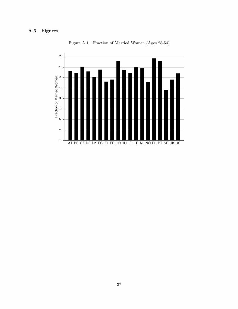
A.6 Figures

Figure A.1: Fraction of Married Women (Ages 25-54)

0.1

.2.3

.4.5

.6.7

.8

Fra

ction o

f M

arr

ied W

om

en

AT BE CZ DE DK ES FI FR GR HU IE IT NL NO PL PT SE UK US

37

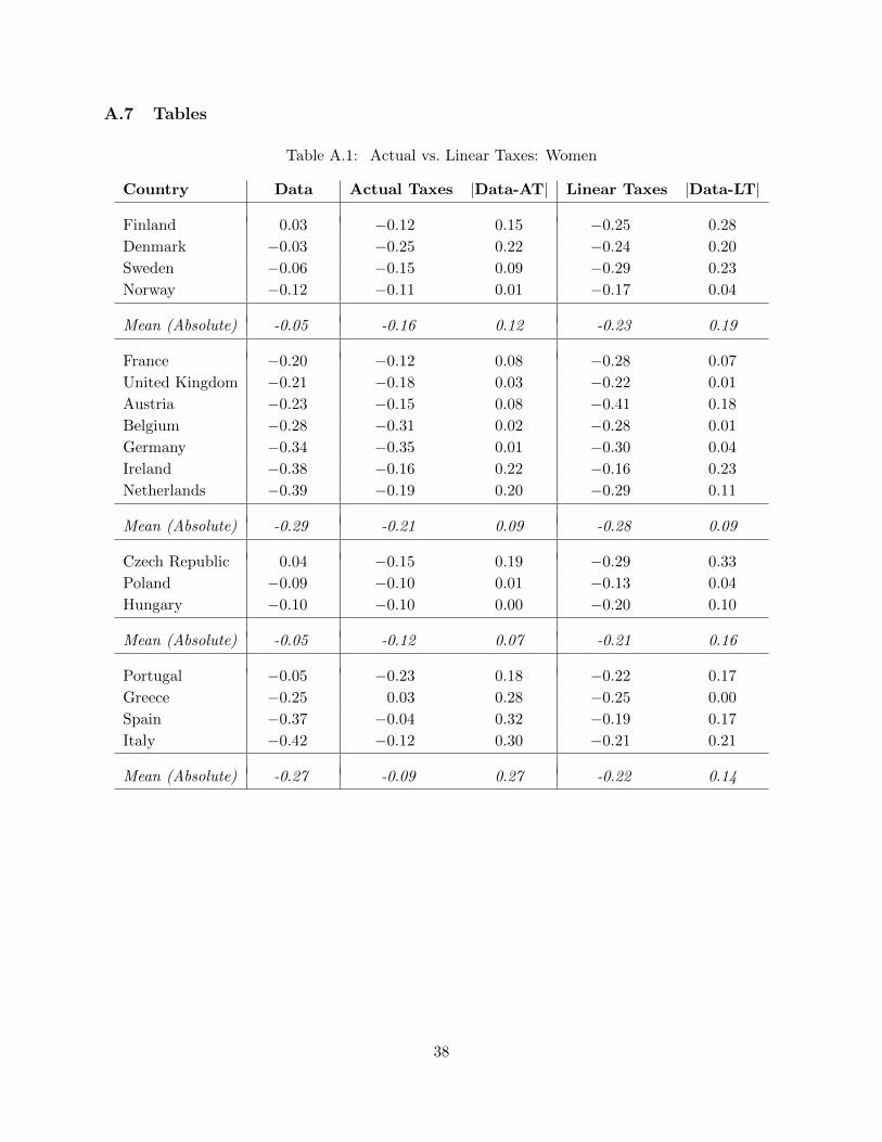
A.7 Tables

Table A.1: Actual vs. Linear Taxes: Women

Country Data Actual Taxes |Data-AT| Linear Taxes |Data-LT|

Finland 0.03 −0.12 0.15 −0.25 0.28

Denmark −0.03 −0.25 0.22 −0.24 0.20

Sweden −0.06 −0.15 0.09 −0.29 0.23

Norway −0.12 −0.11 0.01 −0.17 0.04

Mean (Absolute) -0.05 -0.16 0.12 -0.23 0.19

France −0.20 −0.12 0.08 −0.28 0.07

United Kingdom −0.21 −0.18 0.03 −0.22 0.01

Austria −0.23 −0.15 0.08 −0.41 0.18

Belgium −0.28 −0.31 0.02 −0.28 0.01

Germany −0.34 −0.35 0.01 −0.30 0.04

Ireland −0.38 −0.16 0.22 −0.16 0.23

Netherlands −0.39 −0.19 0.20 −0.29 0.11

Mean (Absolute) -0.29 -0.21 0.09 -0.28 0.09

Czech Republic 0.04 −0.15 0.19 −0.29 0.33

Poland −0.09 −0.10 0.01 −0.13 0.04

Hungary −0.10 −0.10 0.00 −0.20 0.10

Mean (Absolute) -0.05 -0.12 0.07 -0.21 0.16

Portugal −0.05 −0.23 0.18 −0.22 0.17

Greece −0.25 0.03 0.28 −0.25 0.00

Spain −0.37 −0.04 0.32 −0.19 0.17

Italy −0.42 −0.12 0.30 −0.21 0.21

Mean (Absolute) -0.27 -0.09 0.27 -0.22 0.14

38

Table A.2: Actual vs. Linear Taxes: Men

Country Data Actual Taxes |Data-AT| Linear Taxes |Data-LT|

Finland −0.12 −0.13 0.01 −0.10 0.02

Denmark −0.12 −0.14 0.02 −0.10 0.03

Norway −0.14 −0.11 0.03 −0.10 0.04

Sweden −0.15 −0.11 0.05 −0.11 0.04

Mean (Absolute) -0.13 -0.12 0.03 -0.10 0.03

Austria −0.04 −0.11 0.07 −0.07 0.03

United Kingdom −0.05 −0.03 0.03 −0.03 0.02

Netherlands −0.06 −0.10 0.03 −0.06 0.00

Ireland −0.07 −0.03 0.04 −0.03 0.04

Germany −0.12 −0.11 0.01 −0.08 0.04

Belgium −0.15 −0.16 0.01 −0.11 0.03

France −0.16 −0.04 0.12 −0.09 0.07

Mean (Absolute) -0.09 -0.08 0.04 -0.07 0.03

Czech Republic −0.02 −0.04 0.02 −0.07 0.05

Poland −0.13 −0.08 0.05 −0.08 0.05

Hungary −0.20 −0.23 0.03 −0.08 0.12

Mean (Absolute) -0.12 -0.12 0.03 -0.08 0.07

Greece 0.00 −0.06 0.06 −0.04 0.05

Portugal −0.09 −0.04 0.05 −0.03 0.06

Spain −0.09 −0.03 0.07 −0.04 0.05

Italy −0.13 −0.10 0.03 −0.10 0.03

Mean (Absolute) -0.08 -0.06 0.05 -0.05 0.05

39

Table A.3: Decomposing Female Hours Worked Differences Relative to the US

Country Data Model τl τc τl + τcwf

ym

Finland 0.03 −0.13 −0.12 −0.14 −0.23 0.10

Denmark −0.03 −0.27 −0.25 −0.16 −0.37 0.11

Sweden −0.06 −0.13 −0.09 −0.16 −0.23 0.13

Norway −0.12 −0.09 −0.10 −0.15 −0.19 0.16

Mean -0.05 -0.15 -0.14 -0.15 -0.26 0.12

France −0.20 −0.05 −0.04 −0.12 −0.17 0.11

United Kingdom −0.21 −0.17 −0.04 −0.10 −0.14 −0.02

Austria −0.23 −0.16 −0.12 −0.12 −0.14 −0.11

Belgium −0.28 −0.31 −0.31 −0.13 −0.39 0.13

Germany −0.34 −0.35 −0.32 −0.10 −0.39 0.05

Ireland −0.38 −0.13 −0.02 −0.13 −0.13 0.02

Netherlands −0.39 −0.20 −0.18 −0.12 −0.20 −0.01

Mean -0.29 -0.19 -0.15 -0.12 -0.22 0.03

Czech Republic 0.04 −0.16 0.01 −0.13 −0.12 −0.03

Poland −0.09 −0.09 −0.09 −0.14 −0.19 0.14

Hungary −0.10 −0.11 −0.14 −0.14 −0.24 0.16

Mean -0.05 -0.12 -0.08 -0.14 -0.19 0.09

Portugal −0.05 −0.19 −0.07 −0.12 −0.18 0.00

Greece −0.25 −0.01 0.17 −0.11 0.05 −0.07

Spain −0.37 −0.01 0.04 −0.09 −0.03 0.04

Italy −0.42 −0.18 −0.13 −0.12 −0.28 0.14

Mean -0.27 -0.10 0.00 -0.11 -0.11 0.03

Note: Male hours are fixed at country-specific means. For the decomposition (columns 3 to 6), onemodel input is set country-specific at once and the rest are left unchanged at their US values.

40

Table A.4: The Effect of Tax Structure and Average Tax Rates on Female Hours Worked DifferencesRelative to the US (θ)

Country Data τl Tax Structure Average Tax Rate

Finland 0.03 −0.12 −0.06 −0.06

Denmark −0.03 −0.25 −0.04 −0.21

Sweden −0.06 −0.09 0.00 −0.09

Norway −0.12 −0.10 −0.03 −0.07

Mean -0.05 -0.14 -0.03 -0.11

France −0.20 −0.04 −0.01 −0.03

United Kingdom −0.21 −0.04 −0.03 −0.01

Austria −0.23 −0.12 −0.09 −0.03

Belgium −0.28 −0.31 −0.29 −0.02

Germany −0.34 −0.32 −0.18 −0.14

Ireland −0.38 −0.02 −0.13 0.11

Netherlands −0.39 −0.18 −0.13 −0.05

Mean -0.29 -0.15 -0.13 -0.02

Czech Republic 0.04 0.01 −0.03 0.04

Poland −0.09 −0.09 0.05 −0.14

Hungary −0.10 −0.14 −0.07 −0.07

Mean -0.05 -0.08 -0.02 -0.06

Portugal −0.05 −0.07 −0.12 0.05

Greece −0.25 0.17 0.14 0.03

Spain −0.37 0.04 0.00 0.04

Italy −0.42 −0.13 −0.07 −0.06

Mean -0.27 0.00 -0.01 0.01

Note: Male hours are fixed at country-specific means. Columns 3 and 4 add up to Column2. Column 2 corresponds to column 3 in Table A.3.

41

Table A.5: The Effect of Tax Structure and Average Tax Rates on Female Hours Worked DifferencesRelative to the US (κ)

Country Data τl Tax Structure Average Tax Rate

Finland 0.03 −0.12 −0.05 −0.07

Denmark −0.03 −0.25 0.00 −0.25

Sweden −0.06 −0.09 0.01 −0.10

Norway −0.12 −0.10 −0.02 −0.08

Mean -0.05 -0.14 -0.02 -0.12

France −0.20 −0.04 −0.01 −0.03

United Kingdom −0.21 −0.04 −0.03 −0.01

Austria −0.23 −0.12 −0.07 −0.05

Belgium −0.28 −0.31 −0.29 −0.02

Germany −0.34 −0.32 −0.13 −0.19

Ireland −0.38 −0.02 −0.18 0.16

Netherlands −0.39 −0.18 −0.11 −0.07

Mean -0.29 -0.15 -0.12 -0.03

Czech Republic 0.04 0.01 −0.01 0.02

Poland −0.09 −0.09 0.06 −0.15

Hungary −0.10 −0.14 −0.05 −0.09

Mean -0.05 -0.08 0.00 -0.08

Portugal −0.05 −0.07 −0.13 0.06

Greece −0.25 0.17 0.14 0.03

Spain −0.37 0.04 0.00 0.04

Italy −0.42 −0.13 −0.07 −0.06

Mean -0.27 0.00 -0.01 0.01

Note: Male hours are fixed at country-specific means. Columns 3 and 4 add up to Column2. Column 2 corresponds to column 3 in Table A.3.

42

Table A.6: Country-Specific Input Variables for Child Care Costs

Country # Preschool Kids pcc

pcc

wfpcc

pcc

wf

Denmark 1.19 1.33 0.06 5.05 0.24

Finland 1.28 1.20 0.08 8.46 0.56

Norway 1.24 1.93 0.09 7.65 0.36

Sweden 1.34 0.77 0.05 6.52 0.39

Mean 1.26 1.31 0.07 6.92 0.39

Austria 1.22 1.84 0.12 8.00 0.50

Belgium 1.27 2.73 0.14 7.09 0.37

France 1.22 2.90 0.20 6.77 0.46

Ireland 1.30 3.26 0.21 7.83 0.51

Germany 1.27 1.93 0.10 9.15 0.47

Netherlands 1.32 4.40 0.24 8.88 0.49

United Kingdom 1.25 5.47 0.29 8.63 0.47

Mean 1.26 3.22 0.19 8.05 0.47

Czech Republic 1.14 0.41 0.07 3.08 0.50

Hungary 1.20 0.25 0.04 2.54 0.39

Poland 1.18 0.39 0.06 3.28 0.48

Mean 1.17 0.35 0.05 2.97 0.46

Spain 1.15 1.91 0.16 4.46 0.38

Greece 1.19 0.57 0.06 4.89 0.52

Italy 1.15 – – – –

Portugal 1.12 1.09 0.13 2.69 0.33

Mean 1.15 1.19 0.12 4.01 0.41

United States 1.29 2.85 0.16 7.18 0.41

First column: number of preschool children per woman with preschool children; secondcolumn: minimum child care costs (hourly, 2005 US-$); third column: ratio of minimumchild care costs relative to average female wage; fourth column: maximum child carecosts (hourly, 2005 US-$); fifth column: ratio of maximum child care costs relative toaverage female wage

43

Table A.7: Hours Worked Differences of Married Women Without Preschool Children Relative tothe US

Country Data Model

United Kingdom −0.18 −0.19

Austria −0.21 −0.22

France −0.21 −0.05

Germany −0.31 −0.39

Belgium −0.33 −0.36

Ireland −0.39 −0.16

Netherlands −0.41 −0.25

Mean -0.29 -0.23

Portugal −0.12 −0.22

Greece −0.29 −0.01

Spain −0.40 −0.04

Italy −0.44 −0.12

Mean -0.31 -0.10

Czech Republic 0.11 −0.16

Hungary −0.06 −0.14

Poland −0.12 −0.08

Mean -0.02 -0.13

44

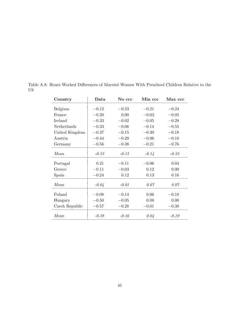
Table A.8: Hours Worked Differences of Married Women With Preschool Children Relative to theUS

Country Data No ccc Min ccc Max ccc

Belgium −0.12 −0.23 −0.21 −0.24

France −0.20 0.00 −0.03 −0.05

Ireland −0.33 −0.02 −0.05 −0.28

Netherlands −0.33 −0.06 −0.14 −0.55

United Kingdom −0.37 −0.15 −0.30 −0.18

Austria −0.44 −0.20 −0.06 −0.18

Germany −0.56 −0.38 −0.21 −0.76

Mean -0.33 -0.15 -0.14 -0.32

Portugal 0.21 −0.11 −0.06 0.04

Greece −0.11 −0.03 0.12 0.00

Spain −0.24 0.12 0.13 0.16

Mean -0.04 -0.01 0.07 0.07

Poland −0.08 −0.14 0.06 −0.18

Hungary −0.50 −0.05 0.08 0.00

Czech Republic −0.57 −0.28 −0.01 −0.38

Mean -0.38 -0.16 0.04 -0.19

45

Table A.9: Hours Worked Differences of Married Men Relative to the US with Wage Heterogeneity

Country Data Homogeneity Heterogeneity

Finland −0.12 −0.13 −0.10

Denmark −0.12 −0.14 −0.13

Norway −0.14 −0.11 −0.10

Sweden −0.15 −0.11 −0.10

Mean -0.13 -0.12 -0.11

Austria −0.04 −0.11 −0.04

United Kingdom −0.05 −0.03 −0.04

Netherlands −0.06 −0.10 −0.06

Ireland −0.07 −0.03 −0.05

Germany −0.12 −0.11 −0.05

Belgium −0.15 −0.16 −0.15

France −0.16 −0.04 −0.01

Mean -0.09 -0.08 -0.06

Czech Republic −0.02 −0.04 −0.01

Poland −0.13 −0.08 −0.06

Hungary −0.20 −0.23 −0.19

Mean -0.12 -0.12 -0.09

Greece 0.00 −0.06 −0.01

Portugal −0.09 −0.04 0.01

Spain −0.09 −0.03 −0.01

Italy −0.13 −0.10 −0.09

Mean -0.08 -0.06 -0.02

46

Table A.10: Hours Worked Differences of Married Women Relative to the US with Wage Hetero-geneity

Country Data Homogeneity Heterogeneity

Finland 0.03 −0.12 −0.04

Denmark −0.03 −0.25 −0.21

Sweden −0.06 −0.15 −0.05

Norway −0.12 −0.11 −0.02

Mean -0.05 -0.16 -0.08

France −0.20 −0.12 −0.07

United Kingdom −0.21 −0.18 −0.10

Austria −0.23 −0.15 −0.26

Belgium −0.28 −0.31 −0.30

Germany −0.34 −0.35 −0.41

Ireland −0.38 −0.16 −0.11

Netherlands −0.39 −0.19 −0.18

Mean -0.29 -0.21 -0.20

Czech Republic 0.04 −0.15 −0.09

Poland −0.09 −0.10 −0.05

Hungary −0.10 −0.10 −0.04

Mean -0.05 -0.12 -0.06

Portugal −0.05 −0.23 −0.12

Greece −0.25 0.03 0.05

Spain −0.37 −0.04 0.07

Italy −0.42 −0.12 −0.13

Mean -0.27 -0.09 -0.03

47

Table A.11: Hours Worked Differences of Married Men Relative to the US With Targeted MaleElasticity εm=0.1

Country Data Baseline εm = 0.1

Finland −0.12 −0.13 −0.09

Denmark −0.12 −0.14 −0.13

Norway −0.14 −0.11 −0.09

Sweden −0.15 −0.11 −0.10

Mean -0.13 -0.12 -0.10

Austria −0.04 −0.11 −0.08

United Kingdom −0.05 −0.03 −0.02

Netherlands −0.06 −0.10 −0.06

Ireland −0.07 −0.03 −0.04

Germany −0.12 −0.11 −0.08

Belgium −0.15 −0.16 −0.11

France −0.16 −0.04 −0.02

Mean -0.09 -0.08 -0.06

Czech Republic −0.02 −0.04 −0.02

Poland −0.13 −0.08 −0.05

Hungary −0.20 −0.23 −0.17

Mean -0.12 -0.12 -0.08

Greece 0.00 −0.06 −0.05

Portugal −0.09 −0.04 −0.03

Spain −0.09 −0.03 −0.02

Italy −0.13 −0.10 −0.07

Mean -0.08 -0.06 -0.04

48

Table A.12: Hours Worked Differences of Married Women Relative to the US With Targeted MaleElasticity εm=0.1

Country Data Baseline εm = 0.1

Finland 0.03 −0.12 −0.12

Denmark −0.03 −0.25 −0.26

Sweden −0.06 −0.15 −0.15

Norway −0.12 −0.11 −0.11

Mean -0.05 -0.16 -0.16

France −0.20 −0.12 −0.15

United Kingdom −0.21 −0.18 −0.18

Austria −0.23 −0.15 −0.14

Belgium −0.28 −0.31 −0.32

Germany −0.34 −0.35 −0.37

Ireland −0.38 −0.16 −0.15

Netherlands −0.39 −0.19 −0.19

Mean -0.29 -0.21 -0.22

Czech Republic 0.04 −0.15 −0.14

Poland −0.09 −0.10 −0.12

Hungary −0.10 −0.10 −0.12

Mean -0.05 -0.12 -0.12

Portugal −0.05 −0.23 −0.23

Greece −0.25 0.03 0.02

Spain −0.37 −0.04 −0.04

Italy −0.42 −0.12 −0.15

Mean -0.27 -0.09 -0.10

49

Table A.13: Hours Worked Differences of Married Men Relative to the US With Different TargetedFemale Elasticities

Country Data Baseline εf = 0.6 εf = 1.0

Finland −0.12 −0.13 −0.15 −0.12

Denmark −0.12 −0.14 −0.16 −0.14

Norway −0.14 −0.11 −0.12 −0.11

Sweden −0.15 −0.11 −0.11 −0.10

Mean -0.13 -0.12 -0.13 -0.12

Austria −0.04 −0.11 −0.12 −0.10

United Kingdom −0.05 −0.03 −0.03 −0.02

Netherlands −0.06 −0.10 −0.11 −0.09

Ireland −0.07 −0.03 −0.04 −0.03

Germany −0.12 −0.11 −0.14 −0.08

Belgium −0.15 −0.16 −0.18 −0.15

France −0.16 −0.04 −0.06 −0.03

Mean -0.09 -0.08 -0.10 -0.07

Czech Republic −0.02 −0.04 −0.05 −0.03

Poland −0.13 −0.08 −0.09 −0.07

Hungary −0.20 −0.23 −0.25 −0.21

Mean -0.12 -0.12 -0.13 -0.10

Greece 0.00 −0.06 −0.07 −0.06

Portugal −0.09 −0.04 −0.05 −0.03

Spain −0.09 −0.03 −0.03 −0.03

Italy −0.13 −0.10 −0.12 −0.08

Mean -0.08 -0.06 -0.07 -0.05

50

Table A.14: Hours Worked Differences of Married Women Relative to the US With DifferentTargeted Female Elasticities

Country Data Baseline εf = 0.6 εf = 1.0

Finland 0.03 −0.12 −0.10 −0.15

Denmark −0.03 −0.25 −0.20 −0.31

Sweden −0.06 −0.15 −0.12 −0.19

Norway −0.12 −0.11 −0.09 −0.13

Mean -0.05 -0.16 -0.13 -0.19

France −0.20 −0.12 −0.09 −0.16

United Kingdom −0.21 −0.18 −0.15 −0.23

Austria −0.23 −0.15 −0.15 −0.15

Belgium −0.28 −0.31 −0.30 −0.35

Germany −0.34 −0.35 −0.28 −0.50

Ireland −0.38 −0.16 −0.13 −0.18

Netherlands −0.39 −0.19 −0.18 −0.21

Mean -0.29 -0.21 -0.18 -0.25

Czech Republic 0.04 −0.15 −0.12 −0.18

Poland −0.09 −0.10 −0.08 −0.15

Hungary −0.10 −0.10 −0.08 −0.12

Mean -0.05 -0.12 -0.09 -0.15

Portugal −0.05 −0.23 −0.19 −0.27

Greece −0.25 0.03 0.03 0.03

Spain −0.37 −0.04 −0.03 −0.05

Italy −0.42 −0.12 −0.10 −0.14

Mean -0.27 -0.09 -0.07 -0.11

51

Table A.15: Hours Worked Differences of Married Women Relative to the US With Country-SpecificRedistribution Factor (λC)

Country Data Baseline λC

Finland 0.03 −0.12 −0.12

Denmark −0.03 −0.25 −0.27

Sweden −0.06 −0.15 −0.16

Norway −0.12 −0.11 −0.11

Mean -0.05 -0.16 -0.16

France −0.20 −0.12 −0.14

United Kingdom −0.21 −0.18 −0.19

Austria −0.23 −0.15 −0.15

Belgium −0.28 −0.31 −0.31

Germany −0.34 −0.35 −0.36

Ireland −0.38 −0.16 −0.18

Netherlands −0.39 −0.19 −0.19

Mean -0.29 -0.21 -0.22

Czech Republic 0.04 −0.15 −0.13

Poland −0.09 −0.10 −0.10

Hungary −0.10 −0.10 −0.09

Mean -0.05 -0.12 -0.11

Portugal −0.05 −0.23 −0.24

Greece −0.25 0.03 0.03

Spain −0.37 −0.04 −0.04

Italy −0.42 −0.12 −0.16

Mean -0.27 -0.09 -0.10

52

Table A.16: Hours Worked Differences of Married Women Relative to the US With AlternativeConsumption Taxes (τMcDaniel

c )

Country Data Baseline τMcDanielc

Finland 0.03 −0.12 −0.11

Denmark −0.03 −0.25 −0.27

Sweden −0.06 −0.15 −0.18

Norway −0.12 −0.11 −0.09

Mean -0.05 -0.16 -0.16

France −0.20 −0.12 −0.14

United Kingdom −0.21 −0.18 −0.16

Austria −0.23 −0.15 −0.15

Belgium −0.28 −0.31 −0.30

Germany −0.34 −0.35 −0.34

Ireland −0.38 −0.16 −0.16

Netherlands −0.39 −0.19 −0.19

Mean -0.29 -0.21 -0.21

Czech Republic 0.04 −0.15 −0.09

Poland −0.09 −0.10 −0.09

Mean -0.03 -0.13 -0.09

Portugal −0.05 −0.23 −0.21

Greece −0.25 0.03 0.08

Spain −0.37 −0.04 −0.02

Italy −0.42 −0.12 −0.16

Mean -0.27 -0.09 -0.08

53

Table A.17: Hours Worked Differences of Married Women Relative to the US With AlternativeWage Measures

Country Data Baseline OECD Wages 1 OECD Wages 2

Finland 0.03 −0.12 −0.11 −0.16

Denmark −0.03 −0.25 −0.25 −0.23

Sweden −0.06 −0.15 −0.17 −0.14

Norway −0.12 −0.11 −0.10 −0.11

Mean -0.05 -0.16 -0.16 -0.16

France −0.20 −0.12 −0.13 –

United Kingdom −0.21 −0.18 −0.18 −0.14

Austria −0.23 −0.15 −0.13 −0.22

Belgium −0.28 −0.31 −0.30 −0.27

Germany −0.34 −0.35 −0.45 −0.42

Ireland −0.38 −0.16 −0.14 –

Netherlands −0.39 −0.19 −0.15 −0.23

Mean -0.29 -0.21 -0.21 -0.26

Czech Republic 0.04 −0.15 −0.14 −0.11

Poland −0.09 −0.10 −0.10 –

Hungary −0.10 −0.10 −0.09 −0.07

Mean -0.05 -0.12 -0.11 -0.09

Portugal −0.05 −0.23 −0.22 −0.02

Greece −0.25 0.03 0.03 0.07

Spain −0.37 −0.04 −0.05 0.05

Italy −0.42 −0.12 −0.23 −0.24

Mean -0.27 -0.09 -0.12 -0.03

54