DISCUSSION PAPER B{212

THE DIRECT APPROACH TO DEBT OPTION PRICING

PUBLISHED IN:

THE REVIEW OF FUTURES MARKETS, VOL.13/2, 1994, PP. 461-515.

SVEN RADY AND KLAUS SANDMANN

Abstract. We review the continuous{time literature on the so{called direct approach to bond option

pricing. Going back to Ball and Torous (1983), this approach models bond price processes directly

(i.e. without reference to interest rates or state variable processes) and applies methods that Black and

Scholes (1973) and Merton (1973) had originally developed for stock options. We describe the principal

modelling problems of the direct approach and compare in detail the solutions proposed in the literature.

1. Introduction

The valuation of debt options, i.e. options written on bonds, has occupied a central place in the litera-

ture on contingent claim pricing and the term structure of interest rates. Despite the fact that commonly

traded debt options are written on coupon bearing bonds, many papers propose pricing formulae for

European options on zero coupon (i.e. pure discount) bonds. There is a speci�c reason for the amount

of research done on these derivatives. Among all interest rate dependent claims, options on zero coupon

bonds most closely resemble options on non{divident paying stocks for which Black and Scholes (1973)

derived their famous pricing formula. Applying the techniques that had been successful with stock op-

tions, several authors were able to obtain solutions as tractable and elegant as the Black{Scholes formula.

On the other hand, discount bond options gain theoretical signi�cance from their role as building blocks

for other derivatives. It is well known, for instance, that caps and oors can be decomposed into strings

of options on zero coupon bonds.1 In some circumstances, it is possible to write the price of a coupon

bond option as a sum of prices of discount bond options.2

There are essentially two approaches to the valuation of bond options: a term structure approach and a

price{based approach.We shall only consider examples where the time parameter is continuous. Within

the term structure approach, analytic formulae for option prices were obtained for instance by Cox,

Ingersoll and Ross (1985), Jamshidian (1989) [ in the term structure model of Vasicek (1977) ], Heath,

Jarrow and Morton (1992) and Longsta� and Schwartz (1992). See below for papers using the price{

based approach. A term structure model aims at describing the price processes of all traded discount

bonds. Typically, these prices are determined as functions of one or more state variables like the short

term interest rate.In Vascicek (1977) and Cox, Ingersoll and Ross (1985), for example, the short rate

is the single state variable. Longsta� and Schwartz (1992) have two state variables, the short rate and

its instantaneous variance. In such a framework, pricing bond options takes two steps. First, prices of

discount bonds must be calculated. This step usually relies on a no{arbitrage argument that guarantees

Date. April 1992. This version: March 22, 1995.

JEL Classi�cation. G13.

Key words and phrases. Arbitrage, Debt Options, Option Pricing.

Both authors are grateful for discussions with Dieter Sondermann and for helpful comments of an anonymous referee.

The usual disclaimers apply.Financial support by Deutsche Forschungsgemeinschaft, Sonderforschungsbereich 303 at the

University of Bonn, is gratefully acknowledged.

1See for instance Sandmann (1991) or Briys, Crouhy and Sch�obel (1991).

2See Jamshidian (1989) and El Karoui and Rochet (1989).

1

2 SVEN RADY AND KLAUS SANDMANN

the existence of so{called market prices of risk for the state variables. These parameters incorporate

investor characteristics such as their attitudes towards risk and must be speci�ed exogenously to close

the model. Once this is done, the prices of bond options are calculated. One constructs a dynamic

trading strategy in bonds that replicates the payo� of the option. According to the law of one price, the

value of the duplicating portfolio and the option price must coincide.

The price{based approach, by contrast, is a one{step procedure starting straight from a model of bond

prices. More precisely, the continuous{time price{based models proposed in the literature specify the

price process of just two bonds: the underlying bond, i.e. the bond on which the option to be valued

is written, and a reference bond, a discount bond of the same maturity as the option. These two bonds

are used to construct a duplicating strategy. As this approach avoids the calculation of bond prices from

state variable processes, it has also been called the direct approach.

In this paper, we review the continuous{time literature on the direct approach. The development of this

literature can be outlined as follows. It starts with Ball and Torous (1983) where the stock option pricing

model of Merton (1973), an extension of Black and Scholes' work that allows for stochastic interest rates,

is adapted to debt options. The main contribution of Ball and Torous consists in replacing the Brownian

motion which drives the Black{Scholes or Merton stock price model by a Brownian bridge process. Thus,

they succeed in modelling the principal di�erence between stocks and bonds: under absence of default

risk, bonds reach a predetermined face value at their maturity whereas stocks have no such target value.

In the Ball{Torous model, the volatility3 of bond prices is constant. As Kemna, de Munnik and Vorst

(1989) note, this implies that the instantaneous variance of a bond's yield grows without bound as the

maturity date approaches. Introducing bond price processes with time dependent volatility, these authors

are able to keep the instantaneous variance of bond yields bounded.

However, the models of Ball and Torous (1983) and Kemna, de Munnik and Vorst (1989) both have

a serious drawback: due to lognormality of bond prices, they assign positive probability to negative

bond yields and negative forward yields. This problem has been addressed by Sch�obel (1986). He

derives boundary conditions for discount bond options under the assumption that yields do not become

negative. Then he proposes a method to modify option price formulae like that of Ball and Torous (1983)

in accordance with these boundary conditions. Yet Sch�obel leaves the underlying bond price model

unchanged; he develops no model in which yields would indeed remain non{negative. B�uhler and K�asler

(1989) were the �rst to achieve this within the direct approach.4 With a very ingenious formulation of

bond prices, their model guarantees positive bond yields as well as positive forward yields and still has

the advantage of providing analytic solutions for option prices.

While the papers mentioned so far deal exclusively with discount bonds, Schaefer and Schwartz (1987)

and B�uhler (1988) use the direct approach to price options on coupon bearing bonds. Both papers let

the volatility of the underlying bond depend on the bond's duration. In such a setting, bond option

prices must be calculated numerically. Unfortunately, both papers make strong assumptions about the

reference bond in order to keep the numerical complexity of the valuation problem at a reasonable level.

Schaefer and Schwartz assume a constant rate of return on the reference bond. B�uhler models this rate as

the underlying bond's yield multiplied by a time dependent factor. It is an advantage of B�uhler's model

that this bond yield always remains positive.

The preceding paragraphs mentioned two of the main modelling problems encountered by the direct

approach: �rst, the problem of specifying bond price processes that reach par value at maturity with

probability one; second, the problem of modelling bond prices in a way that precludes negative yields. A

3Practitioners as well as academic researchers have used the term \volatility" to denote various quantities that measure

the riskiness of an asset. We adopt the following convention:\volatility" is synonymous with \instantaneous standard

deviation of returns".4As for the term structure approach, Cox, Ingersoll and Ross (1985) and Longsta� and Schwartz (1992) are models with

positive yields.

2 PRINCIPAL FEATURES 3

third problem has to do with the internal consistency of models: bond price processes must be speci�ed

such that no arbitrage opportunities between the bonds arise. A su�cient condition for the absence of

arbitrage opportunities is the existence of a so{called martingale measure, i.e. a new probability measure

under which all asset prices, expressed in units of a numeraire asset, can simply be calculated as expected

values of future prices.5 Due to the technical complexity of this question, the existence of a martingale

measure has rarely been investigated within the direct approach.6 Cheng (1991) shows that there is

no such measure for the Ball{Torous model. Reacting to Cheng's work, de Munnik (1990) proves the

existence of a martingale measure for the model of Kemna, de Munnik and Vorst (1989). B�uhler and

K�asler (1989) provide the most elegant solution. While de Munnik's work is technically rather intricate,

B�uhler and K�asler are able to give a straightforward proof that their model admits a martingale measure.

The aim of our paper is to emphasize the above modelling problems and to discuss in detail the di�erent

solutions proposed in the literature. As the problems of the direct approach arise already with the

modelling of zero coupon bonds, we will focus on papers where options on zero coupon bonds are studied.

The remaining sections of the paper are organized as follows. Next, we give a short introduction to the

principal features of discount bonds and discount bond options. The third section reviews the general

framework of the direct approach. We show that the construction of duplicating strategies on forward

rather than spot markets simpli�es the technique and makes the structure of pricing formulae more

transparent. Section 4 and 5 discuss the lognormal models of Ball and Torous (1983) and Kemna, de

Munnik and Vorst (1989), respectively. In section 6, we analyse the modi�ed pricing formulae proposed

by Sch�obel (1987). The model of B�uhler and K�asler (1989) is presented in section 7. Section 8 contains

concluding remarks. Some proofs and technical details are given in an appendix.

2. Principal features of bond prices and debt options

A zero coupon bond pays its owner a predetermined amount of money, the face value, at a predeter-

mined calendar date in the future, the expiration date.7 The face value is usually normalized to one. Our

notation for the time t price of a zero coupon bond which expires at T � t is B(t; T ). As the price of the

bond at maturity has to equal its face value, we get the following terminal value condition:

B(T; T ) = 1 8T :(1)

It is this condition that makes bond price modelling more intricate than stock price modelling.

We may classify bond price models according to whether they generate negative yields or not. De�ning

the yield to maturity Y (t; T ) and the forward yield Y (t; T1; T2) as usual by

B(t; T ) = expf�(T � t) � Y (t; T )g 8 t < T

andB(t; T2)

B(t; T1)= expf�(T2 � T1) � Y (t; T1; T2)g 8 t � T1 < T2 ;

we get

Y (t; T ) < 0, B(t; T ) > 1

and

Y (t; T1; T2) < 0, B(t; T2)

B(t; T1)> 1, B(t; T2) > B(t; T1) :

A simple argument shows that under absence of arbitrage the condition

B(t; T ) � 1 8t; T : t < T(2)

5See Harrison and Pliska (1981) or M�uller (1985). For models using the direct approach, it is convenient to choose the

reference bond as numeraire asset. Asset prices expressed in units of this numeraire are just forward prices.6By contrast, this question has had great in uence on the term structure literature; see in particular Heath, Jarrow and

Morton (1992).

7We consider only bonds without any default risk, e.g. treasury bills.

4 2 PRINCIPAL FEATURES

is equivalent to

B(t; T2) � B(t; T1) 8t; T1; T2 : t � T1 < T2 :(3)

Thus, an arbitrage{free bond price model generates negative yields to maturity if and only if it generates

negative forward yields. In the following, a model that violates (2) and (3) will simply be said to generate

negative yields. We cannot a priori exclude negative yields when considering a bond market without the

possibility of holding cash: Some agents may wish to transfer so much of their wealth into the future

that they are willing to accept negative yields. On the other hand, rational agents who prefer more to

less and are able to hold cash will never engage in a (forward) loan contract with negative yield.8 So a

\realistic" bond model should ful�l (2) and (3).

A European call option on a zero coupon bond expiring at T is the right to buy the bond at some speci�ed

date � < T for some �xed amount K. If the price of the bond at the exercise date � < T is higher than

the exercise price K the net cash ow of the call will be the di�erence B(�; T ) � K, otherwise the net

cash ow is zero. Therefore, at the exercise date � , the call is worth

[B(�; T ) �K]+ := maxf0; B(�; T )�Kg :A European put option is the right to sell a bond for some �xed amount K. The net cash ow of this

option can be written as

[K � B(�; T )]+ := maxf0;K � B(�; T )g :The so{called put{call parity9 describes the relation between today's prices of European call and put

options:

Put[t; B(t; T ); B(t; � ); �;K] = Call[t; B(t; T ); B(t; � ); �;K]�B(t; T ) +K �B(t; � ) :As the net cash ow of an option is always non{negative, put{call parity gives us lower bounds for option

prices, i.e.

Call[t; B(t; T ); B(t; � ); �;K] � maxf0; B(t; T )�K �B(t; � )g :(4)

An upper bound10 for the price of a call is the price of the underlying security itself, so

Call[t; B(t; T ); B(t; � ); �;K] � B(t; T ) :(5)

An additional upper bound holds when there are no negative yields. In this case interesting exercise

prices K lie between 0 and 1 and the maximal payo� of a call is 1 � K. The call price is therefore

bounded from above by the present value of 1�K:

Call[t; B(t; T ); B(t; � ); �;K] � B(t; � ) � (1�K) :(6)

This was �rst observed by Sch�obel (1987). Furthermore, combining (4) and (6), Sch�obel obtains the

following condition for time t call prices whenever B(t; T ) = B(t; � ):

Call[t; B(t; T ) = B(t; � ); B(t; � ); �;K] = B(t; � ) � (1�K) :(7)

Similar results for put options may be derived using put{call parity.

So far no assumptions have been made on the stochastic behaviour of bond prices. But it is already

obvious that the price of an option will not only depend on its underlying bond, but also on the price

B(t; � ) of a zero coupon bond with exactly the same maturity � as the option.11 The bond price based

approach to option pricing studies models in which these two bonds are indeed all that is needed to

determine the option price. This will be discussed in the following section.

8Remember that we are dealing with nominal securities and therefore nominal yields.

9See for example Stoll (1968).

10Boundary conditions (4) and (5) were derived in Merton (1973). For condition (5) see also Gleit (1978).

11This bond will be called the reference bond and its price denoted by R(t) instead of B(t; �).

3 OPTION PRICING BY PORTFOLIO DUPLICATION 5

3. Option pricing by portfolio duplication

We repeat in this section the standard portfolio duplication argument which is the basis of derivative

asset pricing. We shall only treat the special case of a European call option written on a zero coupon

bond with face value 1 and maturity T . The option is assumed to have exercise date � < T and strike

price K. For 0 � t � T; B(t) denotes the time t price of the bond on which the option is written (the

\underlying bond"). The price of the reference bond at time t 2 [0; � ] is denoted by R(t).

Suppose today's bond prices, B(0) and R(0), are known. In order to evaluate the option, we have

to specify the uncertainty governing future price changes, i.e. the nature of the stochastic processes

fB(t)gt2[0;T ] and fR(t)gt2[0;� ]. For the moment, we only assume that these processes are continuous Ito

processes.12

Now, the main idea is to construct a dynamically adjusted portfolio in the two bonds that yields the

same cash ow as the option. To make this more precise, we need some de�nitions:13

A portfolio strategy is represented by a two{dimensional predictable stochastic process � = (�1; �2) on

the time interval [0; � ] such that the stochastic integralsR�1dB and

R�2dR exist. Think of �1(t) and

�2(t) as the number of underlying resp. reference bonds held at time t. Predictability means that the

decision how many bonds to hold at t is based only on information available before t. The stochastic

integrals above can be interpreted as the gains or losses from bond trade according to the strategy �.

The value process of a strategy � is given by

V� := �1B + �2R :

A strategy � is called self{�nancing if V� has the stochastic di�erential

dV� = �1dB + �2dR :

This means that after the initial investment V�(0) is made, the adjustment of the portfolio is �nanced

without injecting or taking out any money. Changes in the portfolio value are exclusively due to gains

or losses from bond trade.

We say a self{�nancing strategy generates the option if the terminal portfolio value equals the cash ow

of the option, i.e.

V�(� ) = [B(� ) �K]+ ;

and V�(t) respects at any time the lower and upper bounds mentioned in section 2, i.e. for all t � �

[B(t) �K �R(t)]+ � V�(t) � B(t)(8)

resp.

[B(t) �K �R(t)]+ � V�(t) � minfB(t); R(t)(1�K)g(9)

if the bond price model precludes negative yields. Then, if there are to be no arbitrage opportunities,14

the option price must indeed coincide with the portfolio value, i.e.

C(t) = V�(t)

for all t 2 [0; � ]. V�(t) is called the arbitrage price of the option.

12An introduction to the theory of such processes and their use in �nance models can be found in Du�e (1992). For

the sake of simplicity, technical requirements such as integrability conditions will not be made explicit here.13We shall not de�ne a space of admissible portfolio strategies as in Harrison{Pliska (1981) or M�uller (1985). But the

strategies we shall deal with can be checked to have the relevant properties.14Formally, an arbitrage opportunity can be de�ned as an admissible self{�nancing portfolio strategy with negative

initial investment, but non{negative �nal value; see for instance Du�e (1992). Thus, an arbitrage opportunity is a trading

strategy that provides a gain today without creating future liabilities.

6 3 OPTION PRICING BY PORTFOLIO DUPLICATION

The construction of a generating strategy can be simpli�ed in the following way. Instead of the two{

dimensional bond price process (B;R), we consider the normalized process (B; 1) where

B :=B

R:

We assume that R�1 is also an Ito process. In the same way, we set

V� :=V�

R= �1B + �2

for the value process of a strategy �. This may look as a purely formal de�nition, but there is an

interesting interpretation. The (B;R){model is a model of the spot markets, so a portfolio strategy �

requires continuous spot trading, i.e. continuous adjustments of long and short positions on the spot

markets for the two bonds, and V� is the spot value process of the strategy. Suppose now that there exist

forward markets at the same time. Then B(t) is just the time t forward price of the underlying bond for

delivery at � (obviously, the corresponding forward price of the reference bond is always 1). If we now

implement our strategy � on the forward markets, the resulting forward value process is just V�. We can

de�ne properties of a strategy � in terms of forward markets: We call � self{�nancing on the forward

markets if

dV� = �1dB ;

and we say such a self{�nancing strategy � generates the option on the forward markets if

V�(� ) = [B(� )�K]+

and V�(t) respects the bounds resulting from division of (8) resp. (9) by R(t). Now a generating strategy

� determines the arbitrage forward price of the option:

C(t) = V�(t) :

The following lemma says that we are free to choose the market we want to work in.

Lemma 1: A portfolio strategy is self{�nancing on the spot markets if and only if it is self{�nancing

on the forward markets. Furthermore, a strategy generates the option on the spot markets if and only if

it generates the option on the forward markets.

The proof of the �rst part consists essentially of an application of Ito's formula and is given in M�uller

(1985) for a more general framework. The second part then follows trivially.

For the construction of a generating strategy in the (B; 1){model of the forward markets, we need an

explicit description of the forward price process fB(t)gt2[0;� ]. We assume that this continuous Ito process

can be described by

dB(t) = �(t) � B(t)dt+ v

�B(t); t

�� B(t)dW (t)(10)

where � is some stochastic process, v(x; t) is a continuous function and W denotes a standard Wiener

process. We call � the drift rate process and v the volatility function of the forward bond price, interpreting

them as instantaneous expectation and standard deviation, respectively, of the in�nitesimal rate of returndB

B. Thus, (10) restricts the volatility of the forward bond to be a deterministic function of the current

forward bond price and time. This restriction, which rules out more complicated dependence of the

forward bond volatility on current or past bond prices B(t) and R(t), will enable us to determine the

arbitrage price of the option.15

Our second lemma shows how to construct generating strategies. Here, the interval I is the state space

of the forward price process B; I is its closure. We assume that either I =]0;1[ or I =]0; 1[.16 In view

of Lemma 1, we do not specify the market where we use the strategy.

15See Jamshidian (1990) for a formulation of the same result in a term structure model.

16This covers all the models we shall deal with except Sch�obel (1987).

3 OPTION PRICING BY PORTFOLIO DUPLICATION 7

Lemma 2: Let u(x; t) be continuous on I � [0; � ] and a solution of the partial di�erential equation

ut(x; t) +1

2v2(x; t)x2uxx(x; t) = 0(11)

on I � [0; � [. Then, the strategy � de�ned by

�1(t) = ux

�B(t); t

�; �2(t) = u

�B(t); t

�� ux

�B(t); t

�� B(t)(12)

is self{�nancing. Moreover, suppose u has the terminal value u(x; � ) = [x�K]+ and satis�es

[x�K]+ � u(x; t) � x if I =]0;1[

or

[x�K]+ � u(x; t) � minfx; 1�Kg if I =]0; 1[ :

Then � generates the call option.

This can be seen as follows. (12) implies V�(t) = u�B(t); t

�. By Ito's formula and (10),

dV�(t) =

�ut

�B(t); t

�+

1

2v2�B(t); t

�� B(t)2 � uxx

�B(t); t

��dt+ ux

�B(t); t

�dB(t):

By (11) and (12), this reduces to dV�(t) = �1dB(t); so � is self{�nancing. The rest is easy to check.

A generating strategy as in lemma 2 yields the arbitrage forward price

C(t) = u�B(t); t

�and the arbitrage spot price

C(t) = R(t) � C(t) = R(t) � u�B(t); t

�for the European call. In accordance with Merton's theory of rational option pricing (1973), the spot

price is homogeneous of degree one in the price B of the underlying security and the discount factor R.

Furthermore, since only the volatility function v appears in the partial di�erential equation (11), the drift

term �(t)B(t) in (10) does not enter the functional relationship between the arbitrage price of the option

and the bond prices B and R.

However, it would be wrong to conclude that the drift is irrelevant for option pricing. When deriving

the above option price, we simply postulated that there are no arbitrage opportunities between traded

securities. The drift of the forward bond price emerges as an important factor when we start to look

for conditions that guarantee the internal consistency of the bond price model (B;R).17 A su�cient

condition for the absence of arbitrage opportunities is the existence of a so{called martingale measure

for the forward bond price. This is a new probability measure that has the same zero probability events

as the original measure and makes the forward price a martingale, which means that at any time the

current forward price is the best estimate of future forward prices. Under such a measure, the forward

value processes of self{�nancing portfolio strategies are martingales as well. In particular, the initial

investment required by a self{�nancing portfolio strategy equals the expectation of the strategy's terminal

value under the martingale measure. As taking expectations preserves non{negativity, a trading strategy

with non{negative �nal value must have a non{negative initial investment. In other words, if there exists

a martingale measure, arbitrage opportunities are precluded.

In the setting described by equation (10), a martingale measure exists if and only if the quotient of the

drift and the volatility of B,�(t)

v(B(t); t)

17In the following, we only try to convey the main ideas. For a thorough discussion including technical details, see for

instance M�uller (1985) or Du�e (1992).

8 3 OPTION PRICING BY PORTFOLIO DUPLICATION

satis�es certain integrability conditions.18 Thus, the internal consistency of a bond price model depends

indeed on both the drift and the volatility of the forward bond price.

There is a second important reason why the drift term matters in option pricing. When applying an

option pricing model, we need estimates for the volatility parameters which enter the valuation formula.

It is in general impossible to estimate these parameters from historical price data without taking into

account the drift as well.19

Let us conclude this section with an example of how the above lemmas are applied. Consider bond price

processes that have the stochastic di�erentials

dB(t) = �B(t) �B(t)dt + �B(t) �B(t)dWB(t)(13)

dR(t) = �R(t) �R(t)dt+ �R(t) �R(t)dWR(t)

with stochastic drift rate processes �B resp. �R but with volatility functions �B and �R depending only

on time t.20 WB and WR are assumed to be Wiener processes having in�nitesimal correlation

dWB(t)dWR(t) = �dt

with constant � 2 [�1; 1].21 After applying Ito's formula to calculate dB(t), it is easy to verify that there

exists a Brownian motion W such that (10) holds with volatility function v : [0; � ]! IR+ given by

v(t)2 = �B(t)2 � 2 � � � �B(t) � �R(t) + �R(t)

2 :

In fact, W can be de�ned by

dW (t) =�B (t)

v(t)dWB(t) � �R(t)

v(t)dWR(t) :

The state space is I =]0;1[. The unique solution of (11) satisfying the terminal value condition and the

bounds speci�ed in lemma 2 is well known:22

u(x; t) = x �N�

1ps

�lnx

K+s

2

���K �N

�1ps

�lnx

K� s

2

��

where N denotes the standard normal distribution function and

s = s(t) =

Z�

t

v(�)2d� :

This yields the familiar formula

C(t) = B(t) �N (d1) �K �R(t) �N (d2)

with

d1=2 =1ps

�ln

B(t)

KR(t)� s

2

�for the arbitrage spot price of a call. It is easy to verify that the generating strategy for the option is

�1 = N (d1) ; �2 = �K �N (d2):

18See Harrison and Kreps (1979), Harrison and Pliska (1983) and M�uller (1985).19A treatment of this estimation problem is beyond the scope of this paper. We therefore refer the reader to Lo

(1986,1988) and references given there. De Munnik (1992) applies Lo's methodology to the model of Kemna, de Munnik

and Vorst (1989). Practitioners often use an \implied volatility approach" to avoid the estimation problem altogether;

inverting the option price formula, they calculate volatility parameters from observed option prices.20This is the framework common to Ball and Torous (1983) and Kemna, de Munnik and Vorst (1989). The models that

Black and Scholes (1973) and Merton (1973) used for stock option pricing can also be seen as special cases of (13).

21The correlation coe�cient � could of course be made time dependent as well.

22The growth condition 0 � u(x; t) � x guarantees uniqueness of the solution; see Gleit (1978).

4 CONSTANT VOLATILITY 9

4. Constant volatility: The Brownian bridge

The �rst approach to price call and put options on zero coupon bonds is due to Ball and Torous (1983).

The starting point of their analysis is the following observation: The Black{Scholes (1973) model of stock

price movements, a geometric Brownian motion

S(t) = S(0) � exp��

�� 1

2�2�� t + � �W (t)

�; �; � constant ;(14)

cannot be reinterpreted as a model for bond prices since this process speci�cation is incompatible with

the face value condition (1). In fact, the variance of the process is strictly increasing with time: V [S(t)] =

S(0)2 � expf2� � tg(expf�2 � tg � 1) :

Ball and Torous for the �rst time incorporated the important face value condition. They model the zero

coupon bond price process fB(t)gt2[0;T ] with maturity T and face value 1 by

B(t) = B(0) � expf�B � t+ �B � �(t; T )g(15)

where f�(t; T )gt2[0;T ] is a standard Brownian bridge,23 i.e. a continuous Gaussian process with

�(0; T ) = �(T; T ) = 0 a.s;

E[�(t; T )] = 0 8t ;

E[�(s; T )�(t; T )] =s(T � t)

T8s < t :

In particular, the variance of the normally distributed random variable �(t; T ) is t(T�t)T

which increases

on [0; T2 ] and decreases on [T2 ; T ]. This bridge process can be constructed as the solution of the stochastic

di�erential equation

d�(t; T ) =��(t; T )T � t dt+ dW (t)

where W is a Brownian motion. Note how the drift pulls the process back to zero. The pull{back force,

� 1T�t

, becomes stronger as time goes by and eventually pulls the process towards its �xed endpoint.

The parameter �B in (15) is now adjusted to ful�l the terminal value condition:

1 = B(T ) = B(0) � expf�B � T + �B � �(T; T )g ) �B = � lnB(0)

T:

�B is just the yield to maturity of the bond at the initial time t = 0. With (15) the bond price process

consists of two parts: the price path that would occur if there were no uncertainty,

B(0) � expf�Btg = B(0)T�tT

and a stochastic drift term driven by �(t; T ) that characterises the random uctuations around this path.

As the distribution of �(t; T ) is symmetric around 0, the deterministic path describes the time t median

of the bond price distribution. B(t) is lognormally distributed with time dependent mean and variance:

E[B(t)] = B(0) � exp��B � t + 1

2�2B �

t(T � t)T

�t!T�! 1

V [B(t)] = B(0)2 � exp�2�B � t+ �2

B� t(T � t)

T

���exp

��2B� t(T � t)

T

�� 1

�t!T�! 0 :

Lognormality obviously implies that at any time 0 < t < T , the price of the zero coupon bond has a

positive probability of exceeding its face value. Thus, negative yields to maturity are generated. But

the Ball{Torous model satis�es the important face value condition. In contrast to the Black{Scholes

model, the density function of the price of the underlying security degenerates at maturity (t = T ).

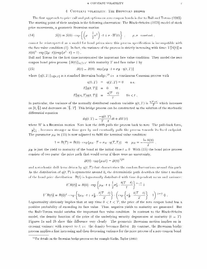
Figures 1a and 1b show this di�erence very clearly. The geometric Brownian motion implies an in-

creasing variance with respect to t; i.e. the density becomes atter. By contrast, the Brownian bridge

process implies a �rst increasing and then decreasing variance for the price process of a zero coupon bond.

23For details on the Brownian bridge process see for example Karlin, Taylor (1981).

10 4 CONSTANT VOLATILITY

0.60.7

0.80.9

11.1

1.2

0.51

1.52

2.5

0

5

10

Figure 1a: Density functions for geometric Brownian motion price process S(t) with T =

3; � = 0:15 , S(0) = 0:785 and � = � ln S(0)T

:

0.70.8

0.91

1.11.2

1.3

0.51

1.52

2.5

1234567

Figure 1b: Density functions for a zero coupon bond price process B(t) as implied by the

Ball{Torous model with T = 3; �B = 0:15 and B(0) = 0:785:

For option pricing, a reference bond with maturity � equal to the exercise date of the option is needed.

Ball and Torous suppose that the price process of the reference bond is of type (15) as well. This leads

to the following model:

B(t) = B(0) expf�B � t+ �B � �(t; T )g = B(0)T�tT � expf�B � �(t; T )g

R(t) = R(0) expf�R � t+ �R � �(t; � )g = R(0)��t� � expf�R � �(t; � )g

with

d�(t; T ) =��(t; T )T � t

dt+ dWB(t)

d�(t; � ) =��(t; � )� � t

dt+ dWR(t)

4 CONSTANT VOLATILITY 11

The instantaneous correlation coe�cient between the Brownian motions WB and WR is assumed to be

constant, i.e.

dWB(t)dWR(t) = �dt :

The forward price B(t) = B(t)R(t) is given by

B(t) = B(0) expf(�B � �R)t+ �B�(t; T )� �R�(t; � )g :Being the quotient of two lognormally distributed variables, it is itself lognormal. Therefore, negative

forward yields have a positive probability at any time t 2]0; � ] :

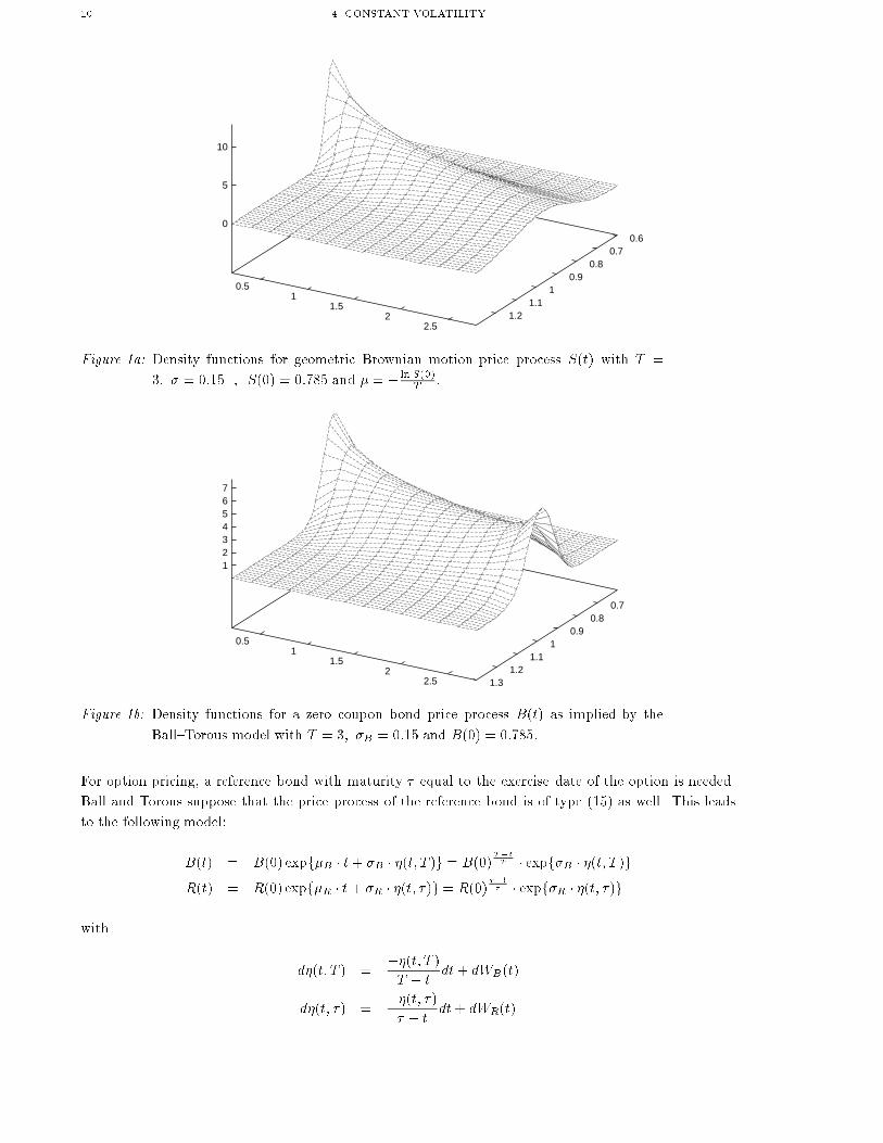
Figure 2: Sample paths of Ball-Torous bond price processes R(t) and B(t) for B(0) =

0:785; R(0) = 0:85; � = 2; T = 3; �R = 0:12; �B = 0:15 and � = 0:75 with

unconditional 95% band.

To illustrate this, consider a symmetric 1� � band for the Brownian bridge process �(t; � ). Since �(t; � )

is normally distributed with variance t(��t)�

the frontiers of the 1�� band are given by ��1��=2q

t(��t)�

for t 2]0; � [ ; i.e. with probability 1� � the realisation of �(t; � ) at time t is contained in this interval.24

Using the relationship between R(t) and �(t; � ), we obtain an unconditional 1� � band for the price of

the reference bond:

a1=2(t) = R(0) exp

(�R � t � �1��=2 � �R �

r(� � t) � t

�

)(16)

That is, prob[a1(t) < R(t) � a2(t)] = 1 � � for all t 2]0; � [ . The unconditional 1 � � band for B(t)

can be calculated in the same way. An example of bond price paths together with unconditional 95%

bands is shown in Figure 2. The paths go above 1, generating negative yields to maturity, and they cross,

generating negative forward yields. The unconditional 95% bands reach also above 1. The same idea can

be used to calculate a conditional 1�� price band for the underlying bond B(t) conditioned on the price

of the reference bond R(t):

b1=2(t) = B(0) �R(t) exp(�B � t+ �

�B

�R�s

(T � t)�(� � t)T �

�lnR(t)� �Rt

�

� �1��=2 � �B �rt(T � t)

T(1� �2)

)(17)

24�1��=2 is the 1� �=2 fractile of the standard normal distribution.

12 4 CONSTANT VOLATILITY

Thus, prob[b1(t) < B(t) � b2(t) j R(t)] = 1� � for all t 2]0; � [ .Returning to option pricing, we calculate the stochastic di�erentials of the bond price processes. By Ito's

Lemma,

dB(t) =

��2B

2� lnB(t)

T � t

�B(t)dt + �BB(t)dWB(t)

dR(t) =

��2R

2� lnR(t)

� � t

�R(t)dt+ �RR(t)dWR(t) :

This is an example of the general speci�cation (13). We can apply the results of section 3 with a constant

volatility function for the forward price,

v(t) =q�2B� 2��B�R + �2

R8t 2 [0; � ] ;

and obtain the arbitrage price of a European call in the Ball{Torous setting:

Call[t; B(t); R(t); �;K] = B(t) �N (d1)�K �R(t) �N (d2)(18)

where

d1=2 =1ps(t)

�ln

B(t)

KR(t)� s(t)

2

�with

s(t) =

Z�

t

(�2B� 2��R�B + �2

R)d� = (�2

B� 2��R�B + �2

R)(� � t) :

The arbitrage price of the European put option is determined by put{call parity:

Put[t; B(t); R(t); �;K] = �B(t) �N (�d1) +K �R(t) �N (�d2):(19)

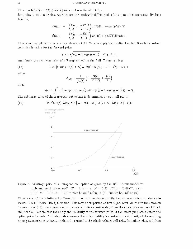
Figure 3: Arbitrage price of a European call option as given by the Ball{Torous model for

di�erent bond prices B(0). T = 3; � = 2; K = 0:92; R(0) = (1:08)�2; �B =

0:15; �R = 0:12; � = 0:75, \lower bound" refers to (4), \upper bound" to (6).

These closed form solutions for European bond options have exactly the same structure as the well{

known Black{Scholes (1973) formulae. This may be surprising at �rst sight: after all, within the common

framework of (13), the above bond price model di�ers considerably from the stock price model of Black

and Scholes. Yet we saw that only the volatility of the forward price of the underlying asset enters the

option price formula. As both models assume that this volatility is constant, the similarity of the resulting

pricing relationships is easily explained. Formally, the Black{Scholes call price formula is obtained from

5 TIME DEPENDENT VOLATILITY 13

(18) by setting �R = 0, i.e. by assuming the reference bond to have a constant yield, and by replacing

B(t) with the stock price.

Despite their formal similarity, the option price formulae derived in the Ball{Torous model and those

calculated in the Black{Scholes model have a fundamentally di�erent theoretical status. While the

latter model possesses a martingale measure25 and hence satis�es su�cient conditions for the absence of

arbitrage opportunities, the Ball{Torous model admits no martingale measure. Cheng (1991) shows that

the drift term of the Brownian bridge which forces the process towards a �xed endpoint is incompatible

with the requirements for the existence of a martingale measure. However, this does not necessarily imply

that there are arbitrage opportunities in the Ball{Torous model: the existence of a martingale measure

is su�cient, but in general not necessary for the absence of arbitrage opportunities.26 To stress the

di�erence between the Black{Scholes and the Ball{Torous model, we might say that pricing in the former

model proceeds safely from su�cient conditions for no arbitrage, whereas pricing in the latter model is

merely based on necessary conditions for no arbitrage: all we have shown is that if the Ball{Torous model

is arbitrage{free, option prices must be given by equations (18) and (19).

On a less theoretical level, one can criticise the Ball{Torous bond price model for the unrealistic yield

behaviour that it implies. This problem, together with a possible solution, will be addressed in the

following section.

5. Time dependent volatility

Using a Brownian bridge, Ball and Torous succeed in specifying a bond price process that satis�es the

terminal value condition, i.e. that reaches par value at maturity. It is instructive to examine the resulting

yield process. (15) implies

Y (t; T ) = � 1

T � t� lnB(t) = �B � �B

T � t� �(t; T ) :(20)

This yield to maturity is normally distributed with mean �B and variance

V [Y (t; T )] =�2B

(T � t)2 � V [�(t; T )] =�2B

(T � t)2� t(T � t)

T=

�2Bt

(T � t)T(21)

which increases without bounds as t tends to T . We can analyse this further by looking at yield changes

over in�nitesimal time periods. The stochastic di�erential of Y (t; T ) is

dY (t; T ) = � �B

(T � t)2 � �(t; T )dt��B

T � td�(t; T ) = � �B

T � tdWB(22)

by Ito's lemmaand the expression for d�(t; T ) given in the previous section. Thus, the di�usion coe�cient

(instantaneous standard deviation) of the yield process explodes as t tends to T . This makes yield

movements over very short time intervals ever more variable and, by adding up, leads to the unbounded

growth of the variance V [Y (t; T )]. Moreover, Kemna, de Munnik and Vorst (1989) point out that the

unbounded di�usion coe�cient causes almost every yield path fY (t; T ) : 0 � t � Tg to reach negative

values. Hence negative yields to maturity are generated with probability 1!

This highlights the serious drawbacks of the Ball{Torous model. One possible way to avoid them is to

replace the Brownian bridge �(t; T ) by a process of the form

~�(t; T ) := k(t; T ) �WB(t) � N�0; k2(t; T ) � t�(23)

25See for example M�uller (1985).26Existence of a martingale measure and absence of arbitrage are equivalent if the state space of the asset price model

is �nite; see Harrison and Pliska (1981). This equivalence breaks down if the state space is in�nite. Back and Pliska (1991)

give an example of a securities market which is arbitrage{free, but has no martingale measure.

14 5 TIME DEPENDENT VOLATILITY

where k(t; T ), a di�erentiable function de�ned for t 2 [0; T ] , is positive for t < T and zero for t = T .

De�ning �B as before and setting

B(t) = B(0) � exp f�B � t+ �B � ~�(t; T )g(24)

one obtains a bond price model that satis�es the terminal value condition. As in Ball and Torous (1983),

the distributions of B(t) and Y (t; T ) are lognormal and normal, respectively. More precisely,

lnB(t) � N���B � (T � t); �2

B� k2(t; T )� ;

Y (t; T ) = �B � �B

T � t � ~�(t; T ) � N

��B;

�2B� k2(t; T )t(T � t)2

�:(25)

The variance of the yield remains bounded as t tends to T if and only if k(t;T )T�t

does so. This is also the

condition for the di�usion coe�cient of Y (t; T ) to stay bounded, as we can see by applying Ito's lemma

twice:

d~�(t; T ) =k0(t; T )

k(t; T )� ~�(t; T )dt+ k(t; T )dWB(26)

and

dY (t; T ) = � �B

(T � t)2 � ~�(t; T )dt��B

T � td~�(t; T )

=

�1

T � t+k0(t; T )

k(t; T )

�� [Y (t; T )� �B ]dt� �B � k(t; T )

T � tdWB(t) :(27)

A model of this type, with k(t; T ) = T�tT

, was proposed by Kemna, de Munnik and Vorst (1989). The

resulting yield process is simply a Brownian motion starting at �B. This model succeeds where the

Ball{Torous model fails. First, yields to maturity have bounded variance. Second, while negative yields

occur with positive probability, as is the case in any model with lognormal bond prices, this probability

is far smaller than 1 for reasonable parameter values. Third, de Munnik (1992) shows that this model

admits a martingale measure and hence precludes arbitrage opportunities.

Turning to the valuation of bond options in a model where bond prices are of the form (24), we use Ito's

formula once more to calculate the stochastic di�erential dB(t; T ). The result is

dB(t) = �B(t) �B(t)dt + �B � k(t; T ) �B(t)dWB (t)(28)

with drift rate process

�B(t) = �B + �B � k0(t; T ) �WB(t) +1

2�2B� k2(t; T ) :(29)

Let R(t), the price of the reference bond, also be of type (24), i.e

R(t) = R(0) � exp f�R � t + �R � ~�(t; � )g(30)

with ~�(t; � ) = k(t; � )WR(t), and assume, as usual, that the instantaneous correlation coe�cient � of the

Wiener processes WB and WR is constant. This is again a special case of (13), and the results of section

3 apply. The volatility of the forward bond price is time dependent:

v(t) =q�2Bk2(t; T )� 2��B�Rk(t; T )k(t; � ) + �2

Rk2(t; � ) :(31)

The arbitrage price for a European call in this situation is again of the familiar form

Call[t; B(t); R(t); �;K] = B(t) �N (d1) �K �R(t) �N (d2)(32)

where d1 and d2 are de�ned as in section 3, with the function s(t) now given by

s(t) = �2B

Z �

t

k2(�; T )d� � 2��B�R

Z �

t

k(�; T )k(�; � )d� + �2R

Z �

t

k2(�; � )d� :(33)

5 TIME DEPENDENT VOLATILITY 15

We have no empirical argument for a special form of the function k(t; T ). On the other hand, it would

be at least of some theoretical interest to compare for example the option prices given by the Ball{

Torous and Kemna{de Munnik{Vorst models. The pricing formulae obtained in these models di�er only

in the de�nition of the function s(t). For a theoretical comparison of option prices, we have to relate

the parameters �B ; �R and � of one model to the corresponding parameters of the other model. There

are many equally plausible (and equally arbitrary) ways to do this. For example, one might impose the

condition that the integral of V [lnB(t)] over the life{time of the bond be the same in both models. For

the Ball{Torous model with volatility parameter �BT for the underlying bond, this integral isZT

0

V [lnB(t)]dt =

ZT

0

�2BT

�T � tT

�tdt = �2BT

T 2

6:

For the Kemna{de Munnik{Vorst bond price process with parameter �KMV , one calculatesZT

0

V [lnB(t)]dt =

ZT

0

�2KMV

�T � t

T

�2tdt = �2KMV

T 2

12:

Requiring these quantities to be equal therefore amounts to imposing the relation

�KMV =p2 �BT :

As shown in Figure 4, this implies that for small t the unconditional variance of lnB(t) (and hence of

B(t) as well) is larger in the Kemna{de Munnik{Vorst model than in the Ball{Torous model, whereas

the reverse holds for t close to the maturity of the bond.

Figure 4: Variance of lnB(t) in the Ball{Torous and Kemna{de Munnik{Vorst model for

B(0) = (1:084)�3; T = 3; �BT = 0:15; �KMV =p2�BT .

Assuming the analogous relationship for the volatility parameter of the reference bond and using the same

correlation coe�cient � in both models, one can now convince oneself that the Kemna{de Munnik{Vorst

price of a European option is higher than the Ball{Torous price if the time di�erence T � � is relatively

large, and smaller than the Ball{Torous price if T � � is relatively small.

While two aws of the Ball{Torous model, namely the exploding variance of the yield to maturity and

the non{existence of a martingale measure, can be remedied by specifying bond price processes with time

dependent volatility, a major problem remains unsolved. In all the models considered so far, yields to

maturity and forward yields can take negative values. This in turn distorts option prices: for example, a

call option written on a zero coupon bond with exercise price equal to the bond's face value has a positive

16 5 TIME DEPENDENT VOLATILITY

price in these models. Sch�obel (1987), B�uhler and K�asler (1989) and K�asler (1991) proposed solutions to

this problem. We shall analyse them in the following two sections.

6. Correcting for negative yields: An absorbing boundary for the forward bond price

We have seen in section 2 that non{negativity of forward yields implies property (7) which states that

the price of a call with strike price K 2 [0; 1] is (1�K)R(t) whenever B(t) = R(t). In terms of forward

prices, (7) says that the forward call price is 1�K whenever B(t) = 1.

The pricing formulae derived in lognormal models such as Ball and Torous (1983) or Kemna, de Munnik

and Vorst (1989) do not ful�l (7), which re ects the fact that these models generate negative yields.

Indeed, the last part of section 3 shows that the call prices calculated in any model which satis�es (10)

with at most time dependent volatility function will violate (7). In this situation, Sch�obel (1987) and

Briys, Crouhy and Sch�obel (1991) propose the alternative call price formula

Call[t; B(t); R(t); �;K] = R(t) � u��t; B(t)

�where u� : [0; � ]� [0; 1]! IR+ solves (11) with time dependent volatility v : [0; � ]! IR+ and satis�es

u�(�; x) = [x�K]+ ;

u�(t; 0) = 0 ;

u�(t; 1) = 1�K :

The �rst equation is the usual terminal value condition. The second equation is a boundary condition

derived from property (5). The third condition is new; it imposes property (7).

Sch�obel solves this problem by transforming it into a heat conduction problem on the non{negative real

half{axis. This transformation is rather complicated. Fortunately, it can be avoided given our knowledge

of the standard case studied in the last part of section 3. Let us write u(t; x;K) for the solution calculated

in section 3 corresponding to exercise price K. For K > 0 and all t, we have

u(t; 1;K) = N

�1ps(� lnK +

s

2)

��K �N

�1ps(� lnK � s

2)

�

u(t; 1;1

K) = N

�1ps(lnK +

s

2)

�� 1

K�N�

1ps(lnK � s

2)

�

where

s = s(t) =

Z �

t

v2(�)d�

as usual. This implies

u(t; 1;K)�K � u(t; 1; 1K) = N

�1ps(� lnK +

s

2)

��K �N

�1ps(� lnK � s

2)

�

�K �N�

1ps(lnK +

s

2)

�+N

�1ps(lnK � s

2)

�= 1�K

since N (�z) + N (z) = 1. Therefore, if we set

u�(t; x;K) = u(t; x;K)�K � u(t; x; 1K)

we clearly get a solution of (11) satisfying the above conditions. More explicitly, we can write

u�(t; x;K) = x �N�d1(t; x;K)

��K �N

�d2(t; x;K)

�� K � x �N

�d1(t; x;

1

K)�+N

�d2(t; x;

1

K)�:

6 CORRECTING FOR NEGATIVE YIELDS 17

This leads to the call price formula

Call[t; B(t); R(t); �;K] = B(t) �N (d1)�K �R(t) �N (d2)

��K �B(t) �N (d3)� R(t) �N (d4)

�(34)

where d1 and d2 are the same as in section 3 and

d3=4 =1ps(t)

�lnKB(t)

R(t)� s(t)

2

�:

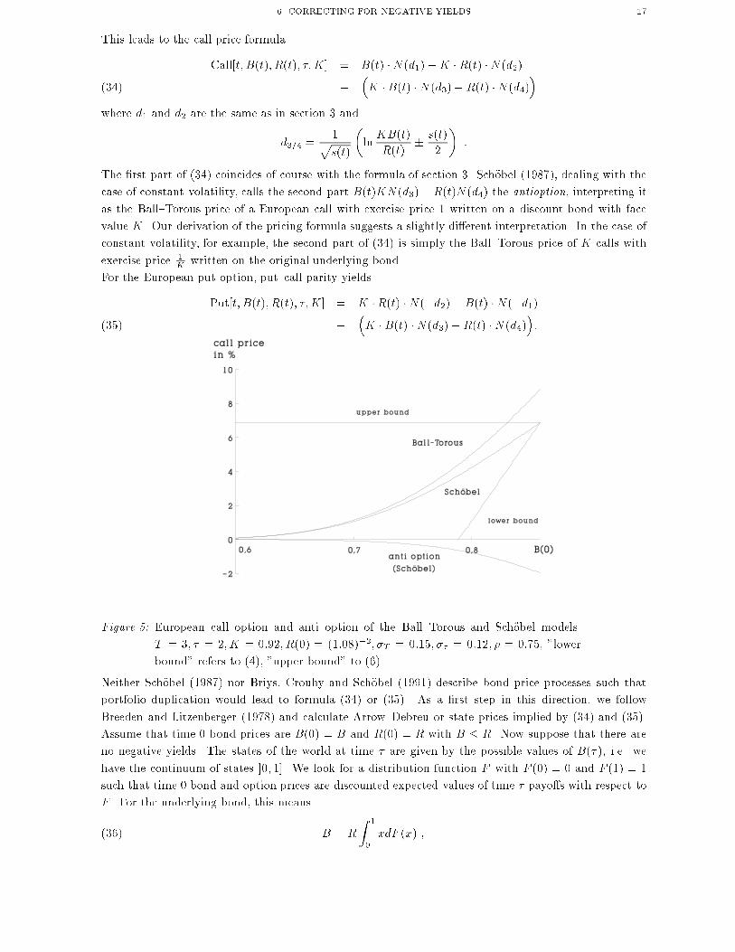
The �rst part of (34) coincides of course with the formula of section 3. Sch�obel (1987), dealing with the

case of constant volatility, calls the second part B(t)KN (d3)�R(t)N (d4) the antioption, interpreting it

as the Ball{Torous price of a European call with exercise price 1 written on a discount bond with face

value K. Our derivation of the pricing formula suggests a slightly di�erent interpretation. In the case of

constant volatility, for example, the second part of (34) is simply the Ball{Torous price of K calls with

exercise price 1K

written on the original underlying bond.

For the European put option, put{call parity yields

Put[t; B(t); R(t); �;K] = K �R(t) �N (�d2)� B(t) �N (�d1)�

�K �B(t) �N (d3) �R(t) �N (d4)

�:(35)

Figure 5: European call option and anti option of the Ball{Torous and Sch�obel models.

T = 3; � = 2;K = 0:92; R(0) = (1:08)�2; �T = 0:15; �� = 0:12; � = 0:75, "lower

bound" refers to (4), "upper bound" to (6).

Neither Sch�obel (1987) nor Briys, Crouhy and Sch�obel (1991) describe bond price processes such that

portfolio duplication would lead to formula (34) or (35). As a �rst step in this direction, we follow

Breeden and Litzenberger (1978) and calculate Arrow{Debreu or state prices implied by (34) and (35).

Assume that time 0 bond prices are B(0) = B and R(0) = R with B � R. Now suppose that there are

no negative yields. The states of the world at time � are given by the possible values of B(� ), i.e. we

have the continuum of states ]0; 1]. We look for a distribution function F with F (0) = 0 and F (1) = 1

such that time 0 bond and option prices are discounted expected values of time � payo�s with respect to

F . For the underlying bond, this means

B = R

Z 1

0

xdF (x) ;(36)

18 6 CORRECTING FOR NEGATIVE YIELDS

and for put options with exercise prices 0 � K � 1,

P (K) = R

Z 1

0

[K � x]+dF (x) = R

ZK

0

(K � x)dF (x)(37)

where we have chosen the simple notation P (K) for the put price Put[0; B;R; �;K] given by (35). The

numberRF (x) can be interpreted as the price of an Arrow{Debreu security IfB(�)�xg paying 1 ifB(� ) � x

and 0 else. (36) and (37) express the consistency of these Arrow{Debreu prices with actual prices of bonds

and options.

Integration by parts yieldsZK

0

(K � x)dF (x) = [(K � x)F (x)]K0 +

ZK

0

F (x)dx =

ZK

0

F (x)dx :

Therefore,

P (K) = R

ZK

0

F (x)dx :

P has continuous derivatives of all orders on ]0; 1[. In particular, F is continuous on ]0; 1[ and satis�es

F (K) =1

R

@P

@K(K) for 0 < K < 1 :

We calculate the derivative of P :

@P

@K= �Bn(�d1)

Kps(0)

+ R �N (�d2) + Rn(�d2)ps(0)

+Rn(d4)

Kps(0)

� B �N (d3)� Bn(d3)ps(0)

= R �N (�d2)� B �N (d3)

where n denotes the standard normal density function.27 Thus,

F (K) = N (�d2)� B

R�N (d3) :(38)

Note that F is continuous at 0: F (K)! 0 for K # 0 . But for K " 1,

F (K)! N

� ln B

R+ 1

2s(0)ps(0)

!� B

R�N ln B

R+ 1

2s(0)ps(0)

!< 1

so F has a jump at 1. On ]0; 1[ , F is continuously di�erentiable. We denote its derivative ]0; 1[ by f and

calculate28

f(K) =@F

@K(K) =

1

Kps(0)

��n(�d2)� B

R� n(d3)

�

=B

R �Kps(0)

� n(d3) �"�

B

R

� 2 lnKs(0)

� 1

#(39)

Note that f is positive on ]0; 1[ since B < R and lnK < 0. Therefore, F is indeed increasing on ]0; 1[. It

can be shown that f(K) ! 0 as K # 0, and the formula for f clearly implies f(K) ! 0 as K " 1.The fact that F has a single jump at the boundary 1 of the state space implies that the Arrow{Debreu

security IfB(�)=1g has a positive price, in contrast to all the other securities IfB(�)=xg with x < 1 having

price zero. Imposing the boundary condition (7) means that probability mass which the original bond

price model places on outcomes B(� ) � 1 has been concentrated in the state B(� ) = 1, so this state

occurs with positive probability. In particular, any bond price model consistent with formulae (34) and

(35) necessarily assigns positive probability to the event that the yield Y (�; T ) becomes zero. Note that

if this happens, there is no reward for holding the underlying bond from � to T .

Using a di�erent method of investigation, Rady (1992) shows that any arbitrage-free bond price model

which does not generate negative yields and supports the option price formulae (34) and (35) necessarily

27Note thatn(�d2)n(�d1)

= BKR

andn(d4)

n(d3)= R

KB.

28We usen(�d2)n(d3)

=�BR

� 2 lnKs(0)

+1

:

7 TIME AND STATE DEPENDENT VOLATILITY 19

has a forward price process B with an absorbing boundary at 1. This boundary is reached with positive

probability.29 In other words, at each time 0 < t � � , there is a positive probability for B(t) = R(t),

and once this has happened, the bond prices coincide until � . Therefore, while satisfying condition (7),

the proposed pricing formulae imply rather implausible bond price behaviour. A more satisfactory model

will be presented in the following section.

7. Beside lognormality: Time and state dependent volatility

In section 5, we have considered models of the type

R(t) = hR(t) � expfgR(t) �WR(t)g

B(t) = hB(t) � expfgB(t) �WB(t)gwith at most time dependent functions hR; hB; gR and gB: hR(t) and hB(t), the median values of R(t)

and B(t), can be interpreted as describing price paths under certainty, whereas the exponential factors

characterise the randommovement around these median paths. Such a model postulates that after taking

the logarithm of bond prices, i.e. after applying the bijective mapping

� : IR2++ �! IR2 ;

�r

b

�7!�ln r

ln b

�;(40)

we are dealing with Gaussian processes. More precisely, the image of the bond prices under � is equal to

the image of the medians plus a Wiener process term with time dependent coe�cients:

�

�R(t)

B(t)

�= �

�hR(t)

hB(t)

�+

�gR(t) �WR(t)

gB(t) �WB(t)

�(41)

The main argument against this approach is that such a model generates negative yields. Indeed, to

ensure positive yields to maturity and forward yields, the bond price vector�R(t)B(t)

�ought to take values

in the triangle

D :=

��r

b

�2 ]0; 1[ 2 : r > b

�:(42)

Given a bijective mapping : D 7! IR2, we can construct a model that has positive yields by rewriting

(41) with rather than �, i.e. by postulating that bond prices satisfy

�R(t)

B(t)

�=

�hR(t)

hB(t)

�+

�gR(t) �WR(t)

gB(t) �WB(t)

�:(43)

The bond prices themselves can be recovered by means of the inverse mapping �1 : IR2 �! D : As

before, hR(t) and hB(t) are the median values of R(t) and B(t).

However, which transformation should we use? There is no obvious choice. Ideally, it would be a simple

mapping that leads to a tractable bond price distribution and closed form solutions for option pricing.

In fact, these goals are achievable, as B�uhler and K�asler (1989) prove with the very ingenuous choice of

the mapping30

: D �! IR2 :

�r

b

�7!�ln r

1�r

ln b

r�b

�:(44)

Its inverse is given by

�1 : IR2 �! D :

�w1

w2

�7!� 1

1+e�w1

1(1+e�w1 )�(1+e�w2 )

�:(45)

29(38) can be interpreted as the transition probability of the forward bond price under a martingale measure. It turns

out that under such a measure, B is a geometric Brownian motion absorbed at 1.30See also K�asler (1991). A one{dimensional variant of this mapping was �rst used by B�uhler (1988) to model the price

process of a coupon bond. See below for a brief discussion of this model.

20 7 TIME AND STATE DEPENDENT VOLATILITY

The resulting bond prices are

R(t) =1

1 + 1�hR(t)

hR(t)expf�gR(t) �WR(t)g

;

(46)

B(t) = R(t) � 1

1 + hR(t)�hB(t)hB(t)

expf�gB(t) �WB(t)g:

Note that the price of the underlying bond depends explicitly on the price of the reference bond. In

particular, both sources of uncertainty,WB andWR, have an impact on the price process of the underlying

bond. By contrast, as B(t) is just a multiple of R(t), the forward bond price has a relatively simple

representation, involving only the Wiener process WB :

B(t) =B(t)

R(t)=

1

1 + hR(t)�hB(t)hB(t)

� expf�gB(t) �WB(t)g(47)

B�uhler and K�asler(1989) develop this model for constant gR and gB ; the generalisation to time dependent

parameters presented here is trivial. Rather than specifying a functional form of hR and hB , they suggest

estimating these functions from the current term structure, but do not go into details. If one wishes to

�x a functional form for hR and hB a priori, one can, for example, proceed in analogy with the models

discussed in previous sections and specify the median paths as

hR(t) := R(0)��t� ;

hB(t) := B(0)T�tT :(48)

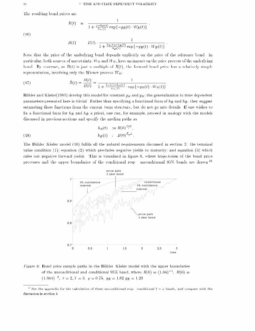
The B�uhler{K�asler model (46) ful�ls all the natural requirements discussed in section 2: the terminal

value condition (1); equation (2) which precludes negative yields to maturity; and equation (3) which

rules out negative forward yields. This is visualised in �gure 6, where trajectories of the bond price

processes and the upper boundaries of the conditional resp. unconditional 95% bands are drawn.31

Figure 6: Bond price sample paths in the B�uhler{K�asler model with the upper boundaries

of the unconditional and conditional 95% band, where R(0) = (1:08)�2; B(0) =

(1:084)�3; � = 2; T = 3; � = 0:75; gR = 1:62 gB = 1:23.

31See the appendix for the calculation of these unconditional resp. conditional 1 � � bands, and compare with the

discussion in section 4.

7 TIME AND STATE DEPENDENT VOLATILITY 21

The distributions of R(t) and B(t) and the conditional distribution of B(t) given R(t) belong to a class

of distributions studied already by Johnson (1946, 1949).32 It is easy to calculate their density functions.

The bond price R(t), for example, has the density function

�(x) =1p2�

1

gR(t)pt

1

x � (1� x)exp

8><>:�

�ln x

1�x � ln hR(t)1�hR(t)

�22tgR(t)2

9>=>; ; x 2]0; 1[:(49)

Johnson has shown that random variables with density functions of this type have �nite moments, but

there are no closed form expressions for them. In addition, one can show (see the appendix) that the

expected value of R(t) is bounded by

1

1 + 1�hR(t)hR(t)

� exp�12gR(t)2t � E[R(t)] � 1

1 + 1�hR(t)hR(t)

� exp��12gR(t)

2t :(50)

For option pricing we need to calculate the stochastic di�erential of the forward price process of the

underlying bond. Ito's formula yields33

dB =

�h0BhR � hBh0R

hB(hR � hB)+ g0

BWB + g2

B

�1

2� B

��B(1� B)dt+ gBB(1� B)dWB:(51)

The volatility of the forward bond price is time and state dependent:

v(x; t) = gB(t) � (1� x)

in the notation of section 3. The state space of B is ]0; 1[. In view of lemma 2, we therefore want to solve

ut(x; t) +1

2g2B(t)x

2(1� x)2uxx(x; t) = 0

on [0; 1]� [0; � ] with the terminal value condition

u(x; � ) = [x�K]+

and the bounds

[x�K]+ � u(x; t) � minfx; 1�Kgin order to determine the arbitrage price for the European call option. It is shown in the appendix how

to solve this problem by transforming it into a heat conduction problem on the real axis. The solution is

u(x; t) = (1�K) � x �N

1ps(t)

�lnx(1�K)

(1 � x)K +s(t)

2

�!

� K � (1� x) �N

1ps(t)

�lnx(1�K)

(1 � x)K � s(t)

2

�!(52)

where N denotes the standard normal distribution function and

s(t) =

Z�

t

gB(�)2d�(53)

Consequently, the B�uhler{K�asler arbitrage price of the European call option is given by:

Call[t; B(t); R(t); �;K] = R(t) � u�B(t)

R(t); t

�(54)

= (1 �K) �B(t) �N (e1) �K ��R(t)� B(t)

��N (e2)

32Johnson constructs classes of distributions by applying the \method of translation" to a standard normal variable Z.

The class of lognormal distributions, for instance, is obtained by means of the exponential transformationZ 7! expf +�Zg.

The transformationZ 7! ( + � expf�Zg)�1 de�nes a class which Johnson denotes by SB . This is the type of distributions

we are dealing with in the B�uhler{K�asler model.

33The time variable t has been omitted to simplify the notation.

22 7 TIME AND STATE DEPENDENT VOLATILITY

with

e1=2 =1ps(t)

�ln

B(t) � (1�K)

(R(t)� B(t)) �K � s(t)

2

�:

The generating strategy for the option is, in the notation of section 3,

�1 = (1�K) �N (e1) +K �N (e2); �2 = �K �N (e2):

The B�uhler{K�asler model (46) is unique within the direct approach in as much as it guarantees positive

yields to maturity as well as positive forward yields and still produces a closed form solution for the

arbitrage price of European debt options. Moreover, B�uhler and K�asler point out that the existence of a

martingale measure is easily demonstrated for the model with constant gR and gB .34

By construction, the pricing formulae of B�uhler and K�asler (1989) and Sch�obel (1987) both satisfy

condition (7):

limB(t)!R(t)Call[t; B(t); R(t); �;K] = (1�K)R(t):

A theoretical comparison of the prices given by these formulae for B(t) < R(t) must, as in section 5, be

based on a hypothetical relationship between the relevant model parameters, i.e. gB on the one hand and

�B; �R and � on the other hand. We assume that these parameters are constant and choose the simplest

approach, postulating that the volatility of the forward bond price at time 0 is the same in both models.

This leads to the relation

gB =

p�2B� 2��B�R + �2

R

1� B(0) :(55)

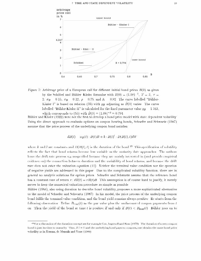
The curve labelled \B�uhler-K�asler I" in Figure 7 has been calculated under this assumption. Thus,

the parameter gB has been adjusted to di�erent initial forward prices. By contrast, the curve labelled

\B�uhler-K�asler II" is based on a single value of gB regardless of B(0).

34It was said in section 3 that a martingale measure exists if and only if the process de�ned as the quotient of the drift

process and the volatility of B satis�es certain integrability conditions. In the model of B�uhler and K�asler (1989), this

process is bounded and hence ful�ls those conditions trivially.

7 TIME AND STATE DEPENDENT VOLATILITY 23

Figure 7: Arbitrage price of a European call for di�erent initial bond prices B(0) as given

by the Sch�obel and B�uhler{K�asler formulae with R(0) = (1:08)�2; T = 3; � =

2; �B = 0:15; �R = 0:12; � = 0:75; and K = 0:92. The curve labelled \B�uhler-

K�asler I" is based on relation (55) with gB adjusting as B(0) varies. The curve

labelled \B�uhler-K�asler II" is calculated for the �xed parameter value gB = 1:343,

which corresponds to (55) with B(0) = (1:08)�3 = 0:794.B�uhler and K�asler (1989) were not the �rst to develop a bond price model with state dependent volatility.

Using the direct approach to evaluate options on coupon bearing bonds, Schaefer and Schwartz (1987)

assume that the price process of the underlying coupon bond satis�es

dB(t) = �B(t) �B(t)dt + k �B(t)l �D(B(t); t)dW

where k and l are constants and D(B(t); t) is the duration of the bond.35 This speci�cation of volatility

re ects the fact that bond returns become less variable as the maturity date approaches. The authors

leave the drift rate process �B unspeci�ed because they are mainly interested in (and provide empirical

evidence on) the connection between duration and the variability of bond returns, and because the drift

rate does not enter the valuation equation (11). Neither the terminal value condition nor the question

of negative yields are addressed in this paper. Due to the complicated volatility function, there are in

general no analytic solutions for option prices. Schaefer and Schwartz assume that the reference bond

has a constant rate of return r: dR(t) = rR(t)dt. This assumption is of course hard to justify, it merely

serves to keep the numerical valuation procedure as simple as possible.

B�uhler (1988), also using duration to describe bond volatility, proposes a more sophisticated alternative

to the model of Schaefer and Schwartz (1987). In his model, the price process of the underlying coupon

bond ful�ls the terminal value condition, and the bond yield remains always positive. He starts from the

following observation. De�ne Bmax(t) as the par value plus the undiscounted coupon payments from t

on. Then the yield of the bond at time t is positive if and only if B(t) < Bmax(t). B�uhler goes on to

35For a discussion of the duration concept see for example Cox, Ingersoll and Ross (1979). The duration of a zero coupon

bond is just its time to maturity. Thus, if l = 1 and the underlying bond pays no coupons, one obtains the same bond price

volatility as in Kemna, de Munnik and Vorst (1989).

24 7 TIME AND STATE DEPENDENT VOLATILITY

construct a bond price process with this property36 and derives the following bond price dynamics:

dB(t) = � lnB(t)

T � t�B(t)dt + k �B(t) � Bmax(t) �B(t)

Bmax(t)� 1 + ��D(B(t); t)dW (t)(56)

with constants k and �. The drift term pulls the process towards the par value (which we have normalised

to one) and away from the boundaries of the state space, 0 and Bmax(t). Again, option prices must be

calculated numerically. Rather than imposing a constant rate of return for the reference bond, B�uhler

simpli�es the numerical procedure by specifying

dR(t) = r(B(t)) �R(t)dt(57)

where r(B(t)) is the yield of the underlying bond multiplied by a time dependent factor. This supposes

perfect positive correlation between the bond yields, which, though far less restrictive than the assumption

made by Schaefer and Schwartz, is still a problematic hypothesis.

It may well be that by relaxing the restrictive assumptions made by Schaefer and Schwartz or B�uhler,

the direct approach could eventually provide a satisfactory valuation model for options on coupon bonds;

the B�uhler model in particular indicates that this would involve considerable technical complications.

The term structure approach seems more appropriate for the pricing of coupon bond options. Modelling

simultaneously the discount bonds of all maturities, this approach can treat coupon bonds simply as

linear combinations of discount bonds. Thus, one encounters no particular modelling di�culties when

moving from discount bonds to coupon bonds. Moreover, there are term stucture models that ensure

positive yields and possess a martingale measure.37 Finally, Jamshidian (1989) and El Karoui and Rochet

(1989) showed that certain term structure models provide tractable formulae for the prices of European

options on coupon bonds: in these models, the price of a coupon bond option can be written as the sum

of the prices of discount bond options. For these reasons, the use of term structure models is generally

seen as the natural approach to the valuation of options on coupon bearing bonds.

8. Conclusion

In this paper, we have given a detailed survey of the direct or price{based approach to debt option

pricing. This approach speci�es bond price processes directly, without relating them to state variables

such as the short term interest rate. The presentation of the portfolio duplication technique in section

3 stresses the fact that the volatility of the forward bond price is the crucial model characteristic for

the calculation of option prices. Therefore, we have structured the paper according to the speci�cation

of volatility, reaching from constant volatility (Ball and Torous (1983)) over time dependent volatility

(Kemna, de Munnik and Vorst (1989)) to time and state dependent volatility (B�uhler and K�asler (1989)).

Focusing on zero coupon bonds, we have emphasized the main modelling problems encountered by the

direct approach: �rst, the problem of specifying bond prices that ful�l the terminal value condition, i.e.

that reach par value at maturity; second, the problem of precluding negative yields to maturity and

negative forward yields; third, the problem of ensuring an arbitrage{free bond price model.

The model of B�uhler and K�asler (1989) is the only one to solve all three problems. Lognormal models

such as Ball and Torous (1983) and Kemna, de Munnik and Vorst (1989) have the advantage of leading

to analytic solutions for bond option prices which are of the same type as the well{known stock option

pricing formulae of Black and Scholes (1973) and Merton (1973). The common weakness of lognormal

models, however, is that negative yields to maturity and negative forward yields occur with positive

probability. As this distorts option prices, Sch�obel (1986) proposes modi�ed pricing formulae. We have

analysed his approach in some detail: imposing an additional constraint on option prices, he implicitely

36This is the �rst example of the transformation method described at the beginning of this section. B�uhler uses a

monotonic mapping to transform a process with values in IR in such a way that the resulting process has the desired

properties.

37See for example Cox, Ingersoll and Ross (1985) or Heath, Jarrow and Morton (1992).

LITERATURE 25

assumes that the forward yield has an absorbing boundary at zero. B�uhler and K�asler (1989), by contrast,

construct a bond price model with positive yields to maturity and positive forward yields that avoids

the implausible assumption of an absorbing boundary and still provides closed form solutions for option

prices.

We have not studied the problems of model testing and parameter estimation. These issues are of course

crucial for the choice of a model and its implementation. For example, a practitioner will prefer a simple

model with some weaknesses to a theoretically more satisfactory model if the parameters of the latter

are much harder to estimate, or if the theoretical weakness of the simple model is negligible for realistic

parameter values.38

Of course, the above models deal only with options on zero coupon bonds and hence are of limited

practical use. As for the valuation of options on coupon bonds using the direct approach, we discussed

the models of Schaefer and Schwartz (1987) and B�uhler (1988). The latter model in particular indicates

that direct modelling of the price process of a coupon bond involves considerable technical complications.

In a term structure model, by contrast, one can easily exploit the fact that a coupon bond is just a

portfolio of discount bonds. We concluded that for the valuation of coupon bond options, the natural

approach is to use a term structure model.

Literature

Back, K.; Pliska, S.R.: (1991): On the Fundamental Theorem of Asset Pricing with an In�nite State Space;

Journal of Mathematical Economics 20, 1-18.

Ball, C.A.; Torous, W.N.: (1983): Bond Price Dynamics and Options; Journal of Financial and Quanti-

tative Analysis 18, 517-531.

Black, F.; Scholes, M.: (1973): The Pricing of Options and Corporate Liabilities; Journal of Political Econ-

omy 81, 637-654.

Breeden, D.; Litzenberger, R.: (1978): Prices of State Contingent Claims Implicit in Option Prices; Jour-

nal of Business 51, 621-651.

Briys, E; Crouhy, M.; Sch�obel, R.: (1991): The Pricing of Default{free Interest Rate Cap, Floor, and

Collar Agreements; Journal of Finance 46, 1879-1892.

B�uhler, W.: (1988): Rationale Bewertung von Optionsrechten auf Anleihen; Zeitschrift f�ur betriebswirtschaftliche

Forschung 10, 851-883.

B�uhler, W.; K�asler, J.: (1989): Konsistente Anleihepreise und Optionen auf Anleihen; working paper, Uni-

versit�at Dortmund, Germany.

Cheng, S.: (1991): On the Feasibility of Arbitrage{Based Option Pricing when Stochastic Bond Price Pro-

cesses are Involved; Journal of Economic Theory 53, 185-198.

Cox, J.C.; Ingersoll, J. jr.; Ross, S.A.: (1979): Duration and the Measurement of Basic Risk; Journal of

Business 52, 51-61.

Cox, J.C.; Ingersoll, J. jr.; Ross, S.A.: (1985): A Theory of the Term Structure of Interest Rates; Econo-

metrica 53; 384-408.

Du�e, D.: (1992): Dynamic Asset Pricing Theory; Princeton, New Jersey: Princeton University Press.

El Karoui, N.; Rochet, J.-C,: (1989): A Pricing Formula for Options on Coupon Bonds; SEEDS Working

Paper 72.

Gleit, A.: (1978): Valuation of General Contingent Claims: Existence, Uniqueness and Comparison of Solu-

tions; Journal of Financial Economics 6, 71-87.

Harrison, J.M.; Kreps, D.M.: (1979): Martingales and Arbitrage in Multiperiod Security Markets; Jour-

nal of Economic Theory 20, 381-408.

38De Munnik (1992) argues along these lines when discussing the model of Kemna, de Munnik and Vorst (1989). He

asserts that the probability of negative yields in this model is very small for realistic parameter values. As a consequence,

the value of a discount bond option with strike price equal to the bond's face value is insigni�cant. Thus, the theoretical

aw of this model turns out to be irrelevant in practice. Moreover, de Munnik indicates that estimating this model is far

easier than estimating the B�uhler{K�asler model.

26 LITERATURE

Harrison, J.M.; Pliska, S.R.: (1981): Martingales and Stochastic Integrals in the Theory of Continuous

Trading; Stochastic Processes and their Application 11, 215-260.

Jamshidian, F.: (1989): An Exact Bond Option Formula; Journal of Finance 44, 205-209.

Jamshidian, F.: (1990): The Preference-Free Determination of Bond and Option Prices from the Spot In-

terest Rate; Advances in Futures and Options Research 4, 51-67.

Johnson, N.L.: (1946): System of Frequency Curves Generated by Methods of Translation; Biometrica,

149-176.

Johnson, N.L.: (1949): Bivariate Distribution Based on Simple Translation Systems; Biometrica, 297-304.

K�asler, J.: (1991): Optionen auf Anleihen; PhD thesis, Universit�at Dortmund, Germany.

Karlin, S.; Taylor, H.M.: (1981): A Second Course in Stochastic Processes; New York: Academic Press.

Kemna, A.G.Z.; de Munnik, J.F.J.; Vorst, A.C.F.: (1989): On Bond Price Models with a Time{Varying

Drift Term; discussion paper, Erasmus Universiteit Rotterdam, Netherlands.

Lo, A.W.: (1986): Statistical Tests of Contingent{Claim Asset{Pricing Models: A New Methodology; Jour-

nal of Financial Economics 17, 143-173.

Lo, A.W.: (1988): Maximum Likelihood Estimation of Generalized Ito Processes with Discretely Sampled

Data; Econometric Theory 4, 231-247.

Longsta�, F.A.; Schwartz, E.S.: (1992): Interest Rate Volatility and the Term Structure: A Two{Factor

General Equilibrium Model; Journal of Finance 47, 1259-1282.

Merton, R.C.: (1973): Theory of Rational Option Pricing; Bell Journal Of Economics and Management 4,

141-183.

de Munnik, J.F.J.: (1992): The Valuation of Interest Rate Derivative Securities; PhD thesis, Tinbergen

Institute Research Series No.40, Netherlands.

M�uller, S.: (1985): Arbitrage Pricing of Contingent Claims; New York: Springer.

Rady, S.: (1992): Forward Yields Implicit in Bond Option Prices; working paper, London School of Econom-

ics.

Sandmann, K.: (1991): Arbitrage und die Bewertung von Zinssatzoptionen; Heidelberg: Physika{Verlag.

Schaefer, S.M.; Schwartz, E.S.: (1987): Time{Dependent Variance and the Pricing of Bond Options;

Journal of Finance 5, 1113-1128.

Sch�obel, R.: (1987): On a Di�erence between Options on Stocks and Default-Free Debt Options: The E�ect

of the Antioption; working paper, Universit�at L�uneburg, Germany.

Stoll, H.R.: (1969): The Relationship between Put and Call Prices; Journal of Finance 24, 802-824.

Vasicek, O.A.: (1977): An Equilibrium Characterization of the Term Structure; Journal of Financial Eco-

nomics 5, 177-188.

Appendix

Unconditional 1� � band of the B�uhler{K�asler model:

1� � = prob [ a1(t) < R(t) � a2(t) ]

= prob

ha1(t) <

1

1 +1�hR(t)

hR(t)expf�gR(t)WR(t)g

� a2(t)

i= prob

hln

a11�a1

� lnhR(t)

1�hR(t)< gR(t) �WR(t) � ln

a2(t)

1�a2(t)� ln

hR(t)

1�hR(t)

iSince gR(t)WR(t) � N(0; gR(t)

2t) the symmetric 1� � intervall for �xed t 2 ]0; � [ is equal to

lna1

1� a1� ln

hR(t)

1� hR(t)=pt gR(t) � ��

2= �

pt gR(t) � �1��

2

, a1(t) =1

1 +1�hR(t)

hR(t)� expf

pt gR(t)�1��

2g

resp. a2(t) =1

1 +1�hR(t)

hR(t)� expf�

pt gR(t)�1��

2g

where �� is the �{fractil of the standard normal distribution.

APPENDIX 27

Conditional 1� � band of the B�uhler{K�asler model:

1� � = prob[b1(t) < B(t) � b2(t)jR(t)]

= prob

�b1(t)

R(t)=: b1(t) < B(t) � b2(t) :=

b2(t)

R(t)

����R(t)�

= prob

"ln

b1(t)

1� b1(t)� ln

hB(t)

hR(t)� hB(t)< gB(t)WR(t)

� ln b2(t)

1� b2(t)� ln hB(t)

hR(t)� hB(t)

�����R(t)#

The conditional distribution of gB(t)WR(t) is N�0; gB(t)

2(1� �2)

�and therefore

b1(t) = R(t)1

1 +hR(t)�hB(t)

hR(t)� expf

pt gB(t)

p1� �2�1��

2g

b2(t) = R(t)1

1 +hR(t)�hB(t)

hR(t)� expf�

pt gB(t)

p1� �2�1��

2g

Upper and lower bounds for the expected value of the zero coupon bond R(t) (B�uhler{K�asler

model):

De�ne � := lnhR(t)

1�hR(t)

� := gR(t)pt

) E[R(t)] =

Z1

0

1p2� �

x

x(1� x)exp

8><>:�

�ln x

1�x � �

�2

2�2

9>=>;dx

=

Z 1�1

1p2� �

1

1 + exexp

�� (x� �)2

2�2

�dx

= 1�Z 1�1

1p2� �

ex

1 + exexp

�� (x� �)2

2�2

�dx

= 1�Z 1�1

1p2� �

1

1 + exexp

8><>:�

�x� (�+ �2)

�2

2�2+ �+

1

2�2

9>=>;dx

= 1� e�+ 1

2�2Z 1�1

1p2� �

1

1 + exexp

�� (x� �� �2)2

2�2

�dx

= 1� e�� 1

2�2Z 1�1

1p2� �

e�2

1 + ex+�2exp

�� (x� �)2

2�2

�dx

� 1� e�� 1

2�2Z 1�1

1p2� �

1

1 + exexp

�� (x� �)2

2�2

�dx

) E[R(t)] � 1

1 + exp��� 1

2�2 =

1

1 +hR(t)

1�hR(t)exp

�� 1

2gR(t)2t

Since the function 1

1+ris convex on [0;+1[ we know from Jensen's inequality

E

"1

1 +hR(t)

1�hR(t)expf�gR(t)W (t)g

#� 1

1 +hR(t)

1�hR(t)E[expf�gR(t)WR(t)g]

=1

1 +hR(t)

1�hR(t)expf 1

2g2R(t)tg

Solution of the B�uhler { K�asler terminal value problem:

ut(x; t) +1

2gB(t)

2x2(1� x)

2uxx(x; t) = 0

u(x; �) = f(x)

28 APPENDIX

This terminal value problem on ]0; 1[ �[0; � ] is transformed by introducing the new time variable

s =

Z �

t

gB(�)2d� ;

the new space variable

z = lnx

1� xor x =

1

1 + e�z

and �nally setting

u(x; t) = a(z)b(s)h(z; s) :

The di�erentiable functions a and b are to be chosen in such a way that any solution h of the heat conduction

equation yields a solution u of the original partial di�erential equation.

One easily calculates the derivatives

zx =1

x(1� x)

zxx =2x� 1

x2(1� x)2

ux = [azh+ ahz]bzx

uxx = fazzh+ 2azhz + ahzz + (2x� 1)[azh+ ahz ]gb 1

x2(1� x)2

ut = a[bsh+ bhs]��g2B(t)

�As

2x� 1 =ez � 1

ez + 1=

ez

2 � e�z

2

ez

2 + e�z

2

= tanhz

2

we get by inserting and dividing by g2B :

ab

�1

2hzz � hs

�+

�az +

1

2a � tanh z

2

�bhz +

�1

2

�azz +

1

2az � tanhz

2

�b� abs

�h = 0 :

In order to make the hz{term vanish, a has to solve the linear di�erential equation

az +1

2a � tanhz

2= 0 :

Separation of variables leads to the solutions

a(z) =c

ez

2 + e�z

2

;

we choose c = 1.

Using the equation for a, one obtains

azz + az � tanh z2= �1

4a :

Therefore, the h{term vanishes if1

8b+ bs = 0 :

We choose the solution

b(s) = e�s

8 :

Result: Setting

u(x; t) =1

ez

2 + e�z

2

e� s

8 h(z; s) ;

we obtain the transformed problem on IR� [0; � ]

1

2hzz � hs = 0;

h(z;0) = (ez

2 + e�z

2 )f

�1

1 + e�z

�:

The solution is:

h(z; s) =1p2�

Z 1�1

h(z + �ps; 0)e

� �2

2 d� :

We omit the explicit formula for u(x; t).

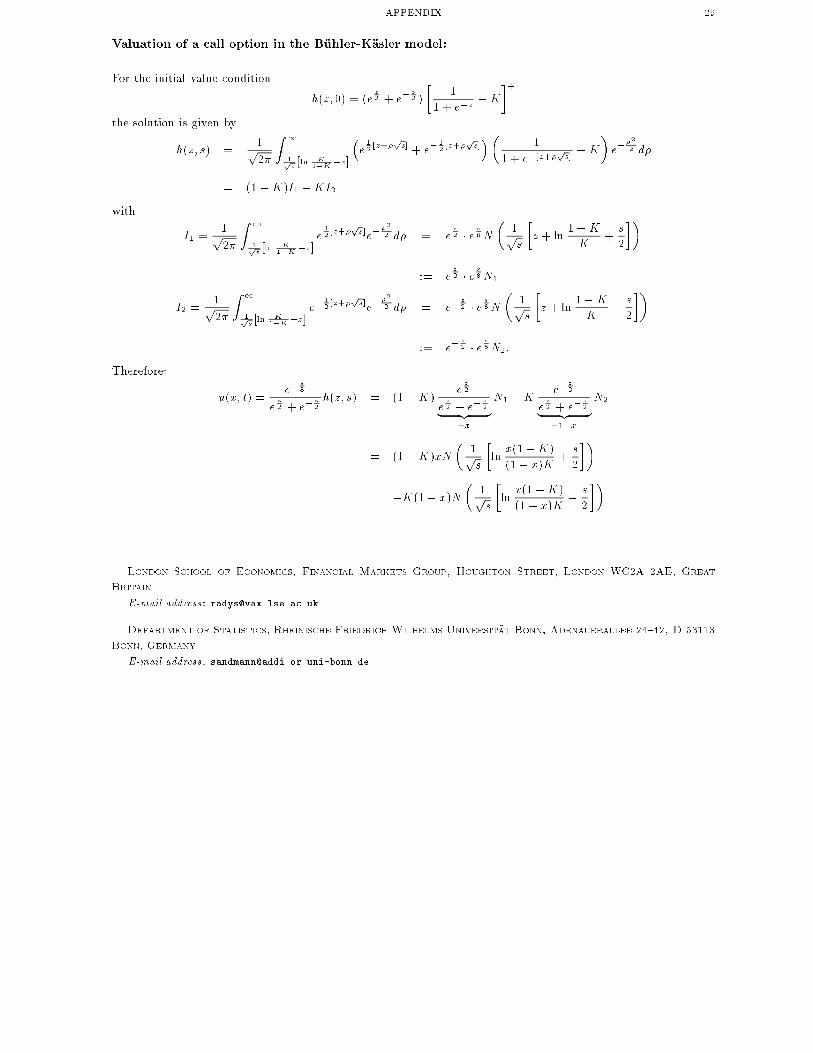
APPENDIX 29

Valuation of a call option in the B�uhler-K�asler model:

For the initial value condition

h(z;0) = (ez

2 + e� z

2 )

�1

1 + e�z�K

�+the solution is given by

h(z; s) =1p2�

Z 11ps[ln K

1�K�z]

�e12[z+�

ps]+ e

� 12[z+�

ps]��

1

1 + e�[z+�ps]�K

�e��

2

2 d�

= (1�K)I1 �KI2

with

I1 =1p2�

Z 11ps[ln K

1�K�z]

e12[z+�

ps]e� �

2

2 d� = ez

2 � e s8N�

1ps

�z + ln

1�K

K+

s

2

��

:= ez

2 � e s8N1

I2 =1p2�

Z 11ps[ln K

1�K�z]

e� 1

2[z+�

ps]e� �

2

2 d� = e� z

2 � e s8N�

1ps

�z + ln

1�K

K� s

2

��

:= e� z

2 � e s8N2:

Therefore:

u(x; t) =e�

s

8

ez

2 + e�z

2

h(z; s) = (1�K)ez

2

ez

2 + e�z

2| {z }=x

N1 �Ke�

z

2

ez

2 + e�z

2| {z }=1�x

N2

= (1�K)xN

�1ps

�ln

x(1�K)

(1� x)K+

s

2

��

�K(1� x)N

�1ps

�ln

x(1�K)

(1� x)K� s

2

��

London School of Economics, Financial Markets Group, Houghton Street, London WC2A 2AE, Great

Britain

E-mail address: radys@vax.lse.ac.uk

Department of Statistics, Rheinische Friedrich-Wilhelms-Universit�at Bonn, Adenauerallee 24{42, D-53113

Bonn, Germany

E-mail address: sandmann@addi.or.uni-bonn.de