Embed Size (px)
DESCRIPTION
Discussion on inheritance: France vs UK vs Sweden 1820-2010. Thomas Piketty Paris School of Economics March 2012. Computing inheritance flow. B t /Y t = µ* t m t W t /Y t ▪ W t /Y t = aggregate wealth/income ratio ▪ m t = aggregate mortality rate - PowerPoint PPT Presentation
Citation preview
Discussion on inheritance: France vs UK vs Sweden
1820-2010
Thomas Piketty
Paris School of Economics
March 2012
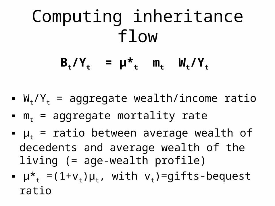
Bt/Yt = µ*t mt Wt/Yt
▪ Wt/Yt = aggregate wealth/income ratio
▪ mt = aggregate mortality rate
▪ µt = ratio between average wealth of decedents and average wealth of the living (= age-wealth profile)
▪ µ*t =(1+vt)µt, with vt)=gifts-bequest ratio
Computing inheritance flow
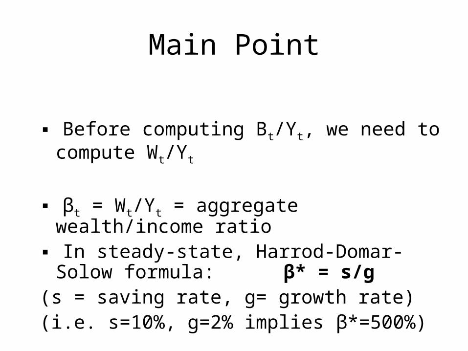
▪ Before computing Bt/Yt, we need to compute Wt/Yt
▪ βt = Wt/Yt = aggregate wealth/income ratio▪ In steady-state, Harrod-Domar-Solow
formula: β* = s/g(s = saving rate, g= growth rate)(i.e. s=10%, g=2% implies β*=500%)
Main Point
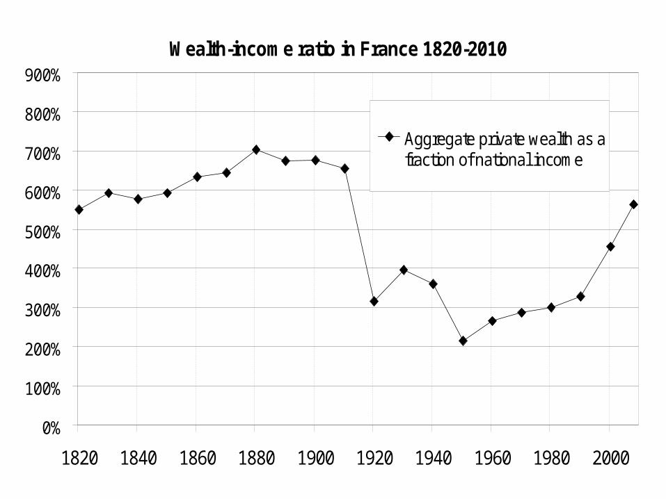
Wealth-income ratio in France 1820-2010
0%
100%
200%
300%
400%
500%
600%
700%
800%
900%
1820 1840 1860 1880 1900 1920 1940 1960 1980 2000
Aggregate private wealth as afraction of national income
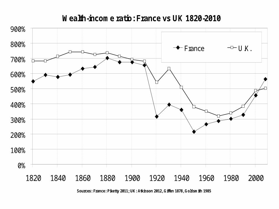
Wealth-income ratio: France vs UK 1820-2010
0%
100%
200%
300%
400%
500%
600%
700%
800%
900%
1820 1840 1860 1880 1900 1920 1940 1960 1980 2000
Sources: France: Piketty 2011; UK: Atkinson 2012, Giffen 1878, Goldsmith 1985
France U.K.
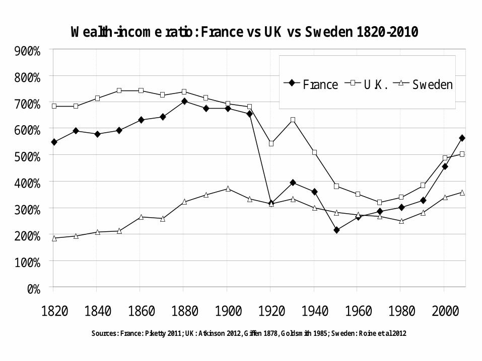
Wealth-income ratio: France vs UK vs Sweden 1820-2010
0%
100%
200%
300%
400%
500%
600%
700%
800%
900%
1820 1840 1860 1880 1900 1920 1940 1960 1980 2000
Sources: France: Piketty 2011; UK: Atkinson 2012, Giffen 1878, Goldsmith 1985; Sweden: Roine et al 2012
France U.K. Sweden

Figure 1: Annual inheritance flow as a fraction of national income, France 1820-2008
0%
4%
8%
12%
16%
20%
24%
28%
32%
36%
40%
1820 1840 1860 1880 1900 1920 1940 1960 1980 2000
Economic flow (computed from national wealth estimates, mortalitytables and observed age-wealth profiles)
Fiscal flow (computed from observed bequest and gift tax data, inc.tax exempt assets)
• There are two ways to become rich: either through one’s own work, or through inheritance
• In the 19th century and early 20th, it was obvious to everybody that the 2nd channel was important: inheritance and successors are everywhere in the literature; huge inheritance flow in tax data
• Q: Does this belong to the past? Did modern growth kill the inheritance channel? E.g. rise of human capital and meritocracy?
• This paper answers « NO » to this question and attempts to explains why, taking France 1820-2050 as an illustration
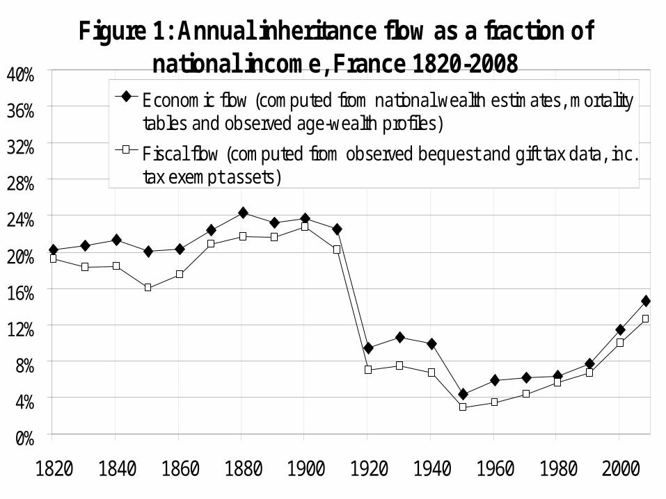
Figure 1: Annual inheritance flow as a fraction of national income, France 1820-2008
0%
4%
8%
12%
16%
20%
24%
28%
32%
36%
40%
1820 1840 1860 1880 1900 1920 1940 1960 1980 2000
Economic flow (computed from national wealth estimates, mortalitytables and observed age-wealth profiles)
Fiscal flow (computed from observed bequest and gift tax data, inc.tax exempt assets)
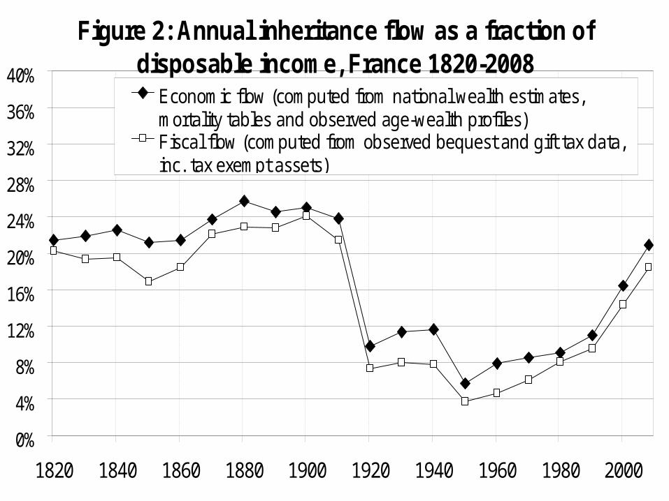
Figure 2: Annual inheritance flow as a fraction of disposable income, France 1820-2008
0%
4%
8%
12%
16%
20%
24%
28%
32%
36%
40%
1820 1840 1860 1880 1900 1920 1940 1960 1980 2000
Economic flow (computed from national wealth estimates,mortality tables and observed age-wealth profiles)Fiscal flow (computed from observed bequest and gift tax data,inc. tax exempt assets)
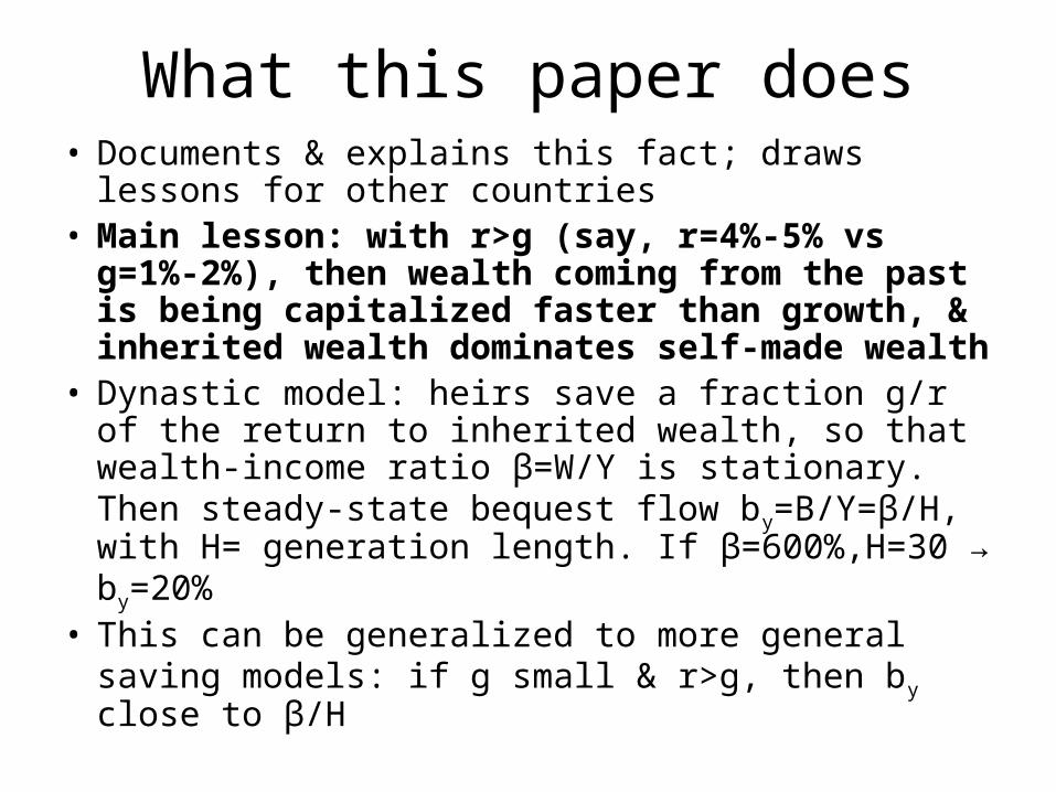
What this paper does• Documents & explains this fact; draws lessons
for other countries• Main lesson: with r>g (say, r=4%-5% vs
g=1%-2%), then wealth coming from the past is being capitalized faster than growth, & inherited wealth dominates self-made wealth
• Dynastic model: heirs save a fraction g/r of the return to inherited wealth, so that wealth-income ratio β=W/Y is stationary. Then steady-state bequest flow by=B/Y=β/H, with H= generation length. If β=600%,H=30 → by=20%
• This can be generalized to more general saving models: if g small & r>g, then by close to β/H
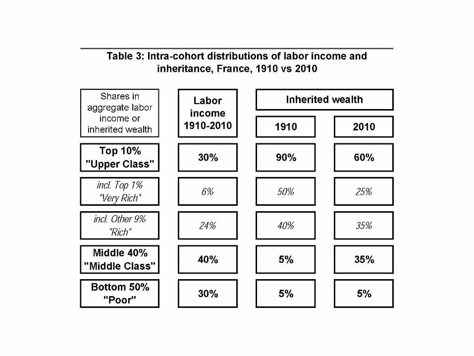
Application to the structure of lifetime inequality
• Top incomes literature: Atkinson-Piketty OUP 2007 & 2010 → 23 countries.. but pb with capital side: we were not able to decompose labor-based vs inheritance-based inequality, i.e. meritocratic vs rentier societies
→ This paper = positive aggregate analysis; but building block for future work with heterogenity, inequality & optimal taxation
Data sources• Estate tax data: aggregate data 1826-
1964; tabulations by estate & age brackets 1902-1964; national micro-files 1977-1984-1987-1994-2000-2006; Paris micro-files 1807-1932
• National wealth and income accounts: Insee official series 1949-2009; linked up with various series 1820-1949
• French estate tax data is exceptionally good: universal, fully integrated bequest and gift tax since 1791
• Key feature: everybody has to fill a return, even with very low estates
• 350,000 estate tax returns/year in 1900s and 2000s, i.e. 65% of the 500,000 decedents (US: < 2%)
(memo: bottom 50% wealth share < 10%)
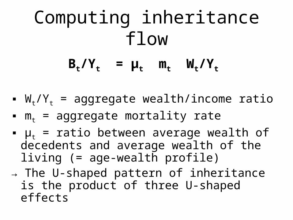
Bt/Yt = µt mt Wt/Yt
▪ Wt/Yt = aggregate wealth/income ratio
▪ mt = aggregate mortality rate
▪ µt = ratio between average wealth of decedents and average wealth of the living (= age-wealth profile)
→ The U-shaped pattern of inheritance is the product of three U-shaped effects
Computing inheritance flow

Figure 1: Annual inheritance flow as a fraction of national income, France 1820-2008
0%
4%
8%
12%
16%
20%
24%
28%
32%
36%
40%
1820 1840 1860 1880 1900 1920 1940 1960 1980 2000
Economic flow (computed from national wealth estimates, mortalitytables and observed age-wealth profiles)
Fiscal flow (computed from observed bequest and gift tax data, inc.tax exempt assets)
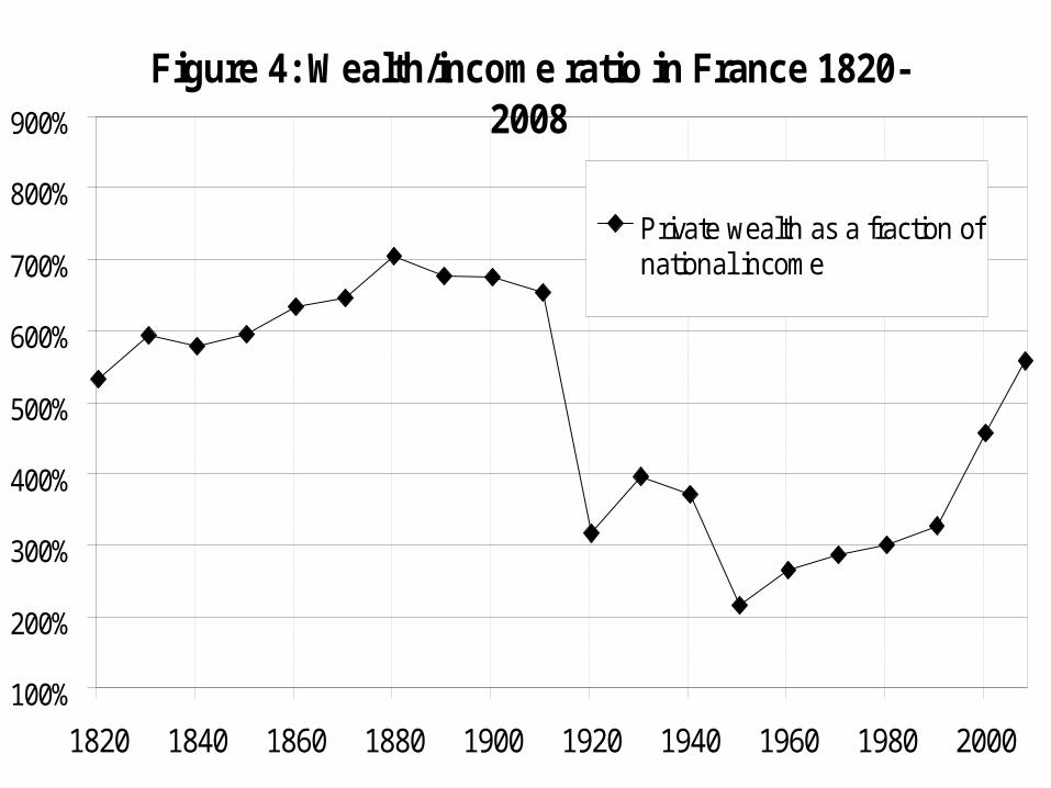
Figure 4: Wealth/income ratio in France 1820-2008
100%
200%
300%
400%
500%
600%
700%
800%
900%
1820 1840 1860 1880 1900 1920 1940 1960 1980 2000
Private wealth as a fraction ofnational income
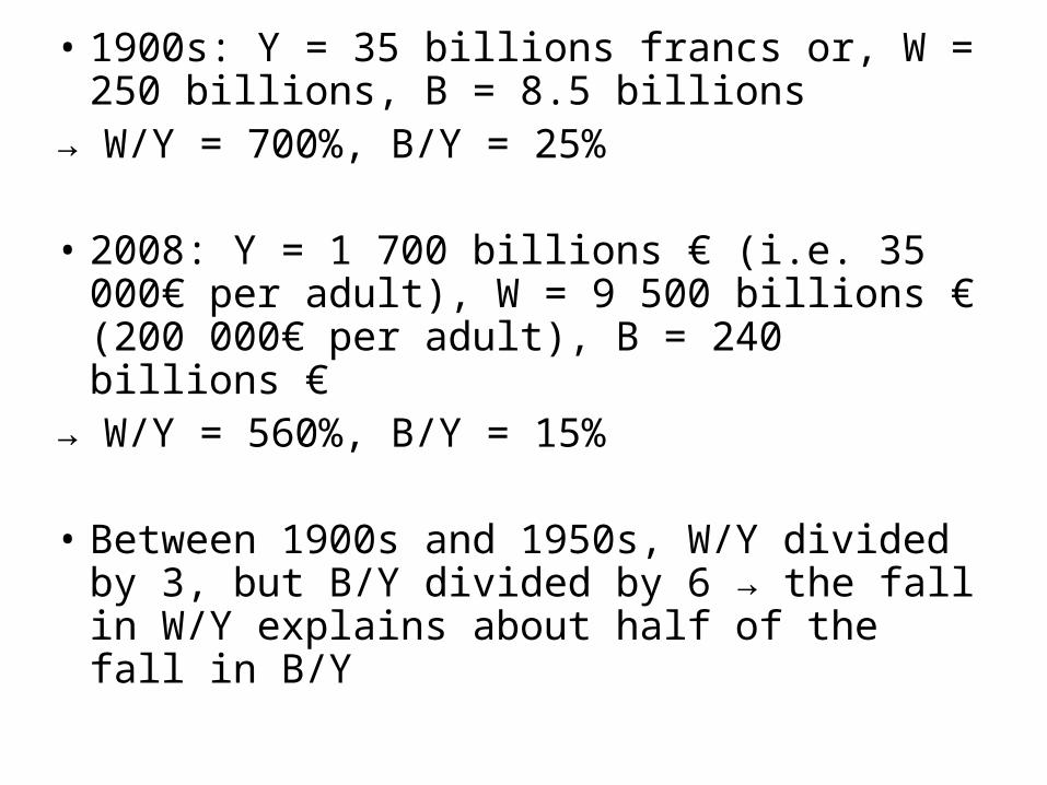
• 1900s: Y = 35 billions francs or, W = 250 billions, B = 8.5 billions
→ W/Y = 700%, B/Y = 25%
• 2008: Y = 1 700 billions € (i.e. 35 000€ per adult), W = 9 500 billions € (200 000€ per adult), B = 240 billions €
→ W/Y = 560%, B/Y = 15%
• Between 1900s and 1950s, W/Y divided by 3, but B/Y divided by 6 → the fall in W/Y explains about half of the fall in B/Y
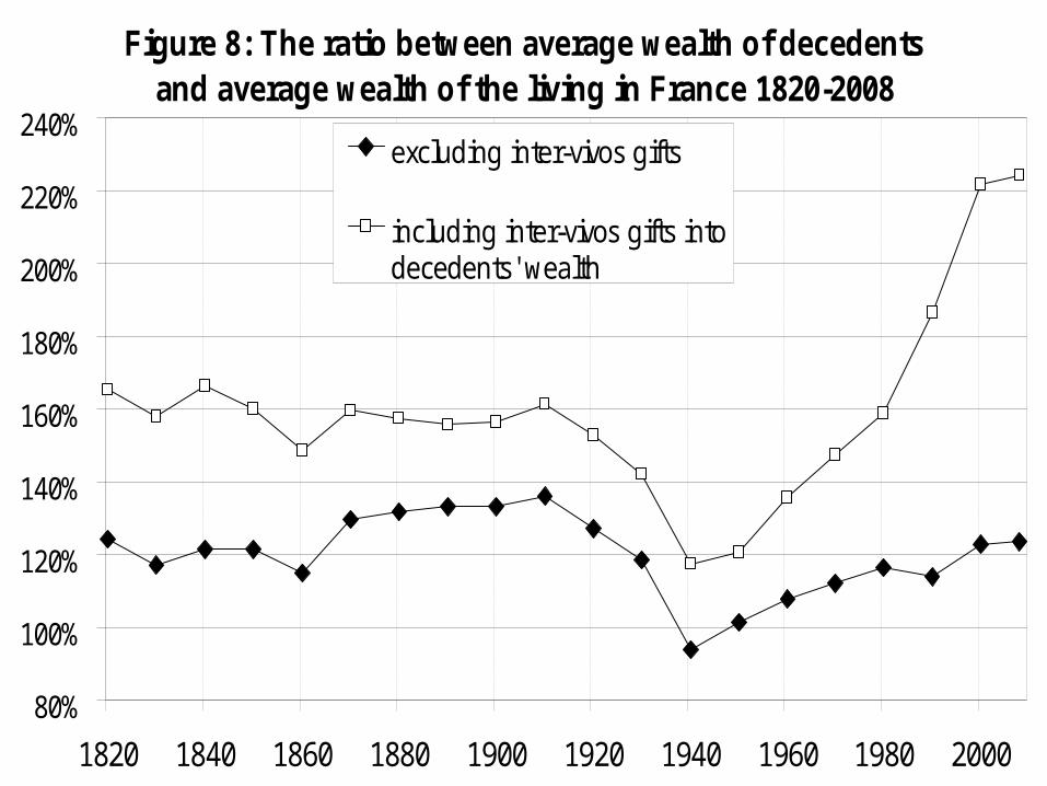
Figure 8: The ratio between average wealth of decedents and average wealth of the living in France 1820-2008
80%
100%
120%
140%
160%
180%
200%
220%
240%
1820 1840 1860 1880 1900 1920 1940 1960 1980 2000
excluding inter-vivos gifts
including inter-vivos gifts intodecedents' wealth
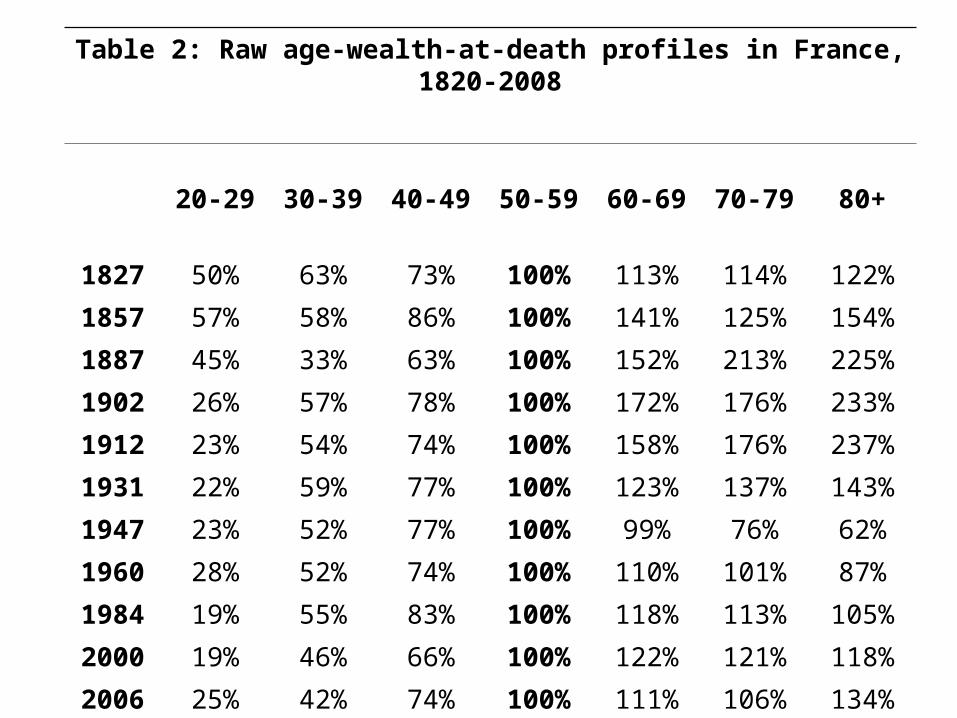
Table 2: Raw age-wealth-at-death profiles in France, 1820-2008
20-29 30-39 40-49 50-59 60-69 70-79 80+
1827 50% 63% 73% 100% 113% 114% 122%
1857 57% 58% 86% 100% 141% 125% 154%
1887 45% 33% 63% 100% 152% 213% 225%
1902 26% 57% 78% 100% 172% 176% 233%
1912 23% 54% 74% 100% 158% 176% 237%
1931 22% 59% 77% 100% 123% 137% 143%
1947 23% 52% 77% 100% 99% 76% 62%
1960 28% 52% 74% 100% 110% 101% 87%
1984 19% 55% 83% 100% 118% 113% 105%
2000 19% 46% 66% 100% 122% 121% 118%
2006 25% 42% 74% 100% 111% 106% 134%
How can we account for these facts?
• 1914-45 capital shocks played a big role, and it took a long time to recover
• Key question: why does the age-wealth profile become upward-sloping again?
→ the r>g effect• Where does the B/Y=20%-25% magic
number come from? Why µt ↑ seem to compensate exactly mt ↓?
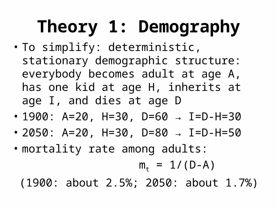
Theory 1: Demography• To simplify: deterministic, stationary
demographic structure: everybody becomes adult at age A, has one kid at age H, inherits at age I, and dies at age D
• 1900: A=20, H=30, D=60 → I=D-H=30
• 2050: A=20, H=30, D=80 → I=D-H=50
• mortality rate among adults:
mt = 1/(D-A)
(1900: about 2.5%; 2050: about 1.7%)
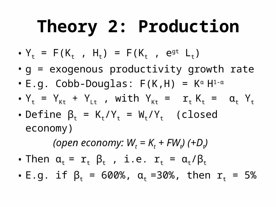
• Yt = F(Kt , Ht) = F(Kt , egt Lt)
• g = exogenous productivity growth rate• E.g. Cobb-Douglas: F(K,H) = Kα H1-α
• Yt = YKt + YLt , with YKt = rt Kt = αt Yt
• Define βt = Kt/Yt = Wt/Yt (closed economy)
(open economy: Wt = Kt + FWt) (+Dt)
• Then αt = rt βt , i.e. rt = αt/βt
• E.g. if βt = 600%, αt =30%, then rt = 5%
Theory 2: Production
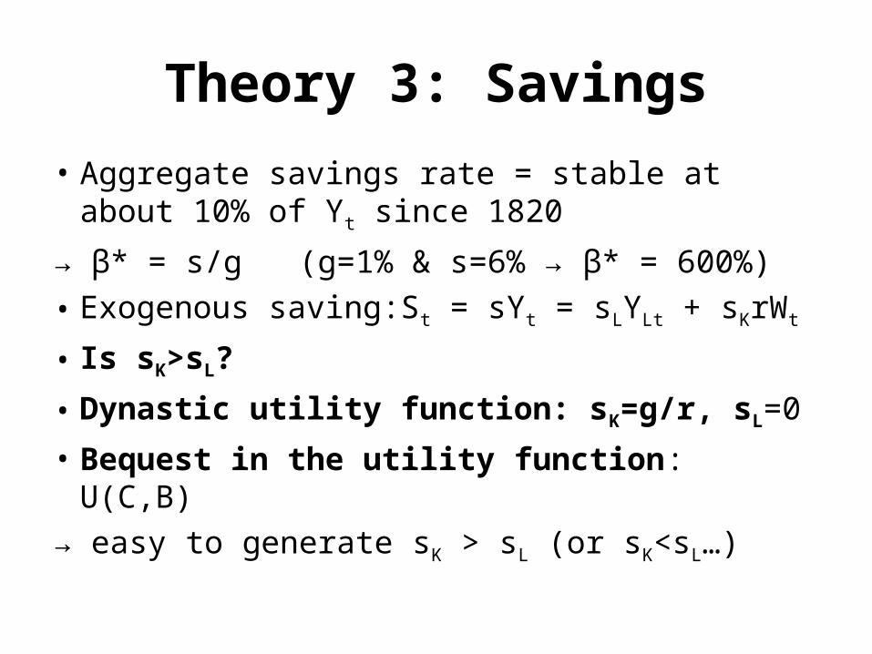
• Aggregate savings rate = stable at about 10% of Yt since 1820
→ β* = s/g (g=1% & s=6% → β* = 600%)
• Exogenous saving:St = sYt = sLYLt + sKrWt
• Is sK>sL?
• Dynastic utility function: sK=g/r, sL=0
• Bequest in the utility function: U(C,B)
→ easy to generate sK > sL (or sK<sL…)
Theory 3: Savings
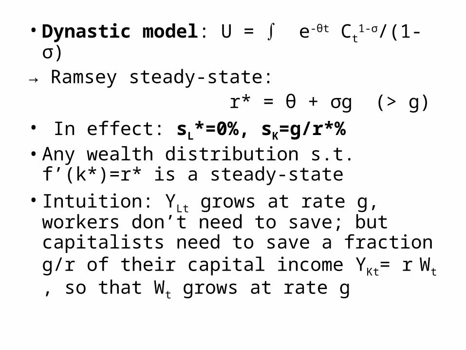
• Dynastic model: U = ∫ e-θt Ct1-σ/(1-σ)
→ Ramsey steady-state: r* = θ + σg (> g)• In effect: sL*=0%, sK=g/r*%• Any wealth distribution s.t. f’(k*)=r* is
a steady-state• Intuition: YLt grows at rate g, workers
don’t need to save; but capitalists need to save a fraction g/r of their capital income YKt= r Wt , so that Wt grows at rate g
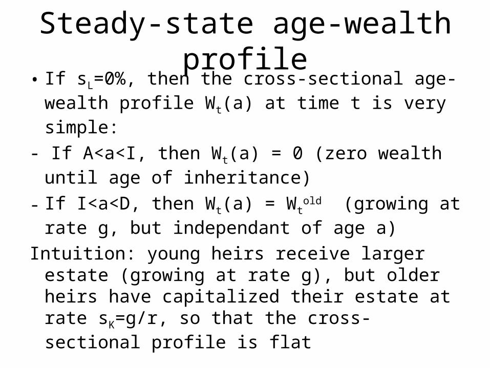
Steady-state age-wealth profile• If sL=0%, then the cross-sectional age-
wealth profile Wt(a) at time t is very simple:
- If A<a<I, then Wt(a) = 0 (zero wealth until age of inheritance)
- If I<a<D, then Wt(a) = Wtold (growing at
rate g, but independant of age a)
Intuition: young heirs receive larger estate (growing at rate g), but older heirs have capitalized their estate at rate sK=g/r, so that the cross-sectional profile is flat
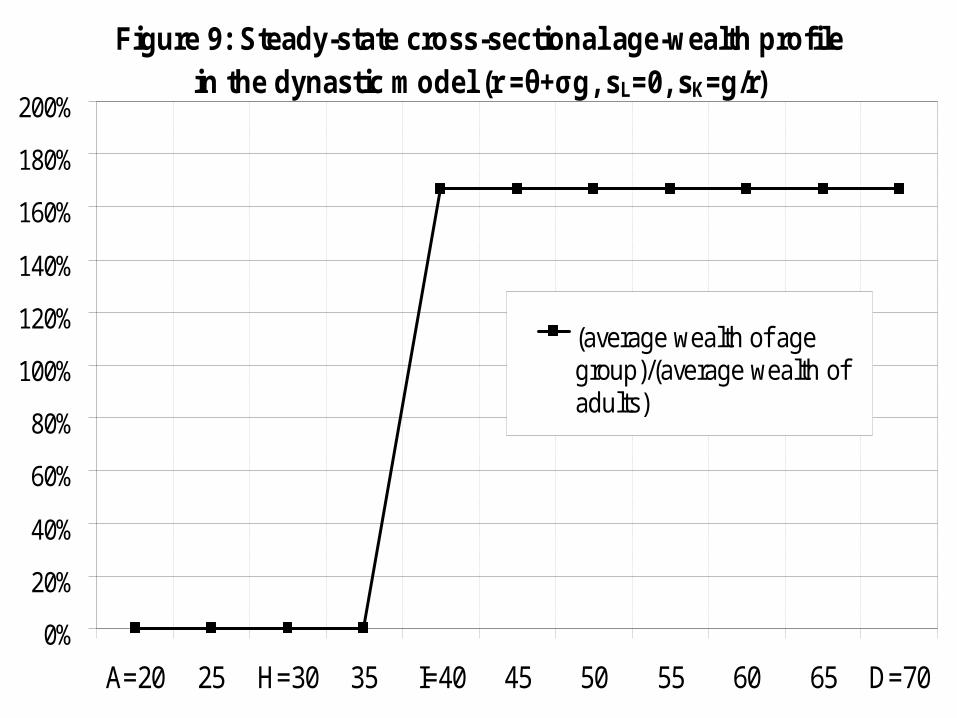
Figure 9: Steady-state cross-sectional age-wealth profile in the dynastic model (r =θ+σg, sL=0, sK=g/r)
0%
20%
40%
60%
80%
100%
120%
140%
160%
180%
200%
A=20 25 H=30 35 I=40 45 50 55 60 65 D=70
(average wealth of agegroup)/(average wealth ofadults)
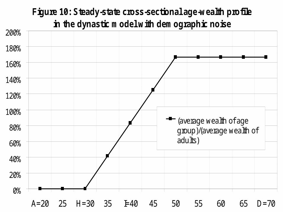
Figure 10: Steady-state cross-sectional age-wealth profile in the dynastic model with demographic noise
0%
20%
40%
60%
80%
100%
120%
140%
160%
180%
200%
A=20 25 H=30 35 I=40 45 50 55 60 65 D=70
(average wealth of agegroup)/(average wealth ofadults)
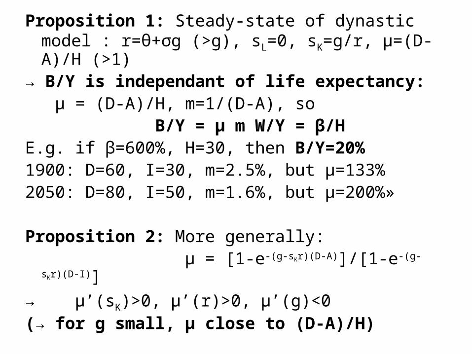
Proposition 1: Steady-state of dynastic model : r=θ+σg (>g), sL=0, sK=g/r, µ=(D-A)/H (>1)
→ B/Y is independant of life expectancy: µ = (D-A)/H, m=1/(D-A), so B/Y = µ m W/Y = β/HE.g. if β=600%, H=30, then B/Y=20%1900: D=60, I=30, m=2.5%, but µ=133% 2050: D=80, I=50, m=1.6%, but µ=200%»
Proposition 2: More generally: µ = [1-e-(g-sKr)(D-A)]/[1-e-(g-sKr)(D-I)]
→ µ’(sK)>0, µ’(r)>0, µ’(g)<0(→ for g small, µ close to (D-A)/H)
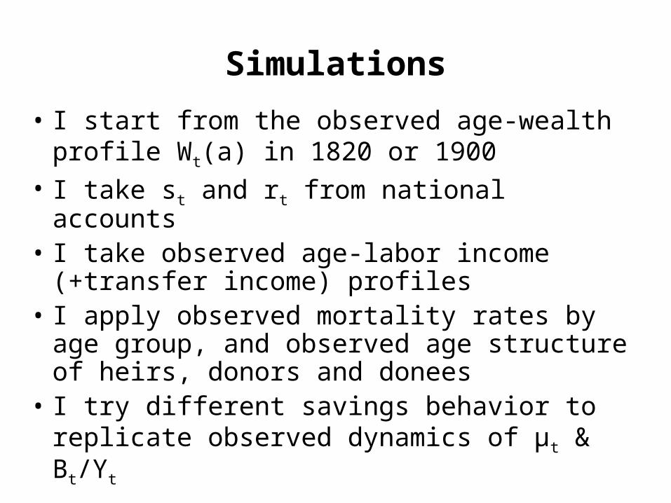
Simulations
• I start from the observed age-wealth profile Wt(a) in 1820 or 1900
• I take st and rt from national accounts• I take observed age-labor income
(+transfer income) profiles• I apply observed mortality rates by age
group, and observed age structure of heirs, donors and donees
• I try different savings behavior to replicate observed dynamics of µt & Bt/Yt
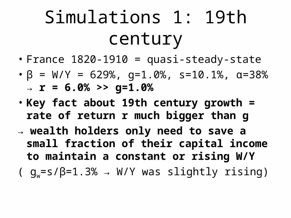
Simulations 1: 19th century
• France 1820-1910 = quasi-steady-state
• β = W/Y = 629%, g=1.0%, s=10.1%, α=38% → r = 6.0% >> g=1.0%
• Key fact about 19th century growth = rate of return r much bigger than g
→ wealth holders only need to save a small fraction of their capital income to maintain a constant or rising W/Y
( gw=s/β=1.3% → W/Y was slightly rising)
→ in order to reproduce both the 1820-1910 pattern of B/Y and the observed age-wealth profile (rising at high ages), one needs to assume that most of the savings came from capital income (i.e. sL close to 0 and sK close to g/r)
(consistent with high wealth concentration of the time)
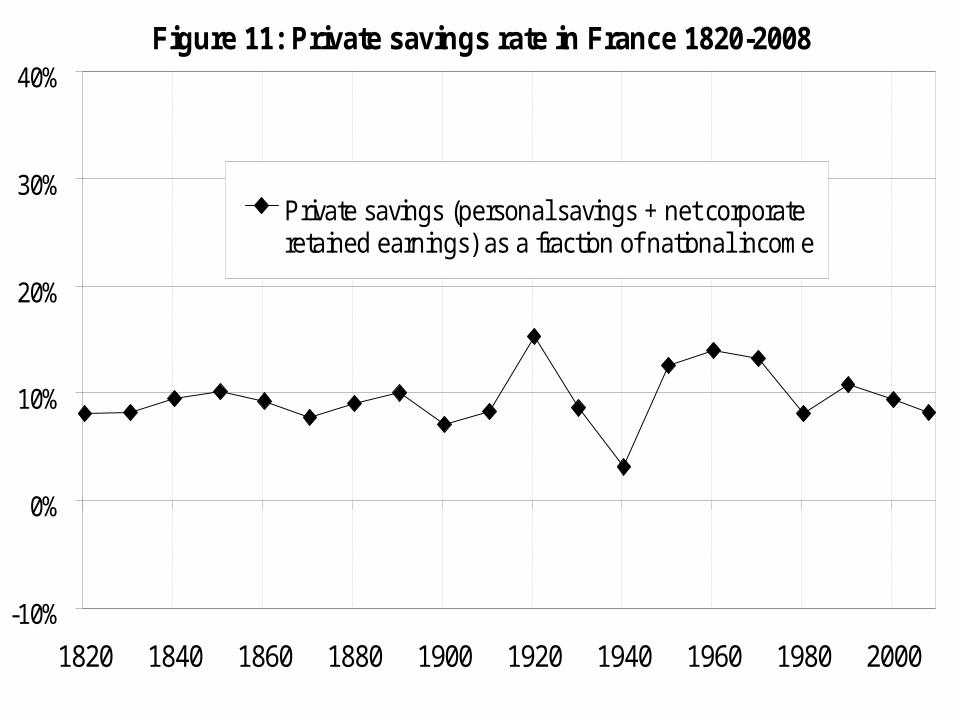
Figure 11: Private savings rate in France 1820-2008
-10%
0%
10%
20%
30%
40%
1820 1840 1860 1880 1900 1920 1940 1960 1980 2000
Private savings (personal savings + net corporateretained earnings) as a fraction of national income
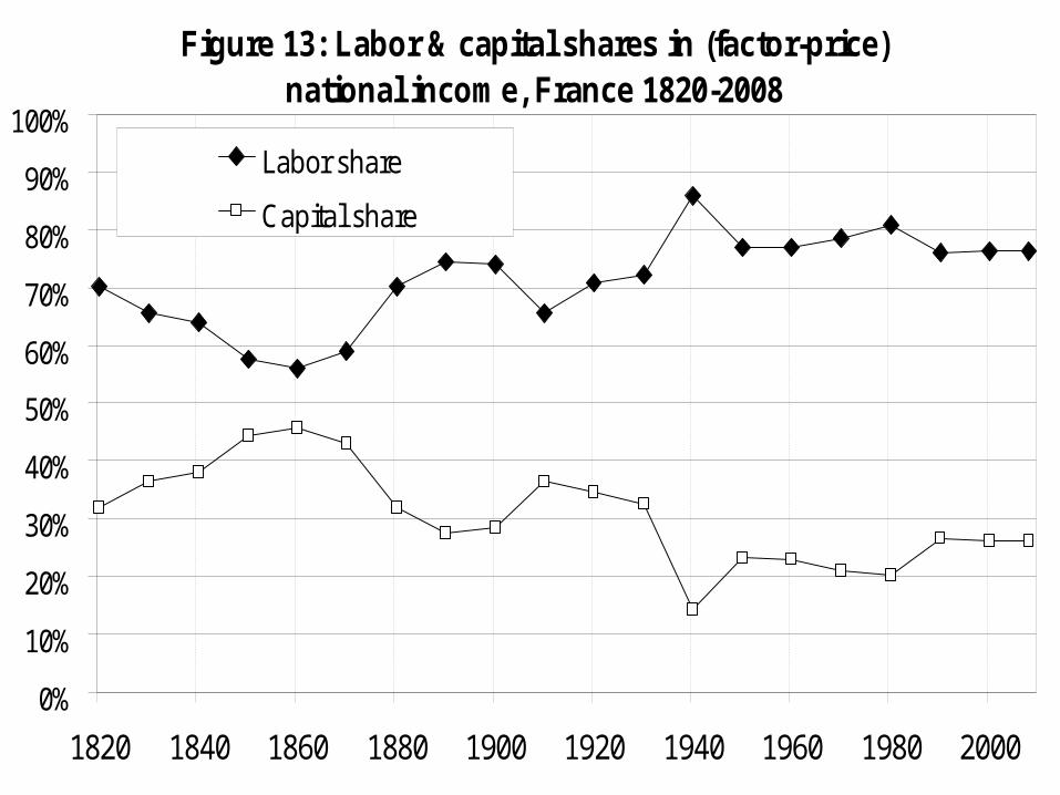
Figure 13: Labor & capital shares in (factor-price) national income, France 1820-2008
0%
10%
20%
30%
40%
50%
60%
70%
80%
90%
100%
1820 1840 1860 1880 1900 1920 1940 1960 1980 2000
Labor share
Capital share
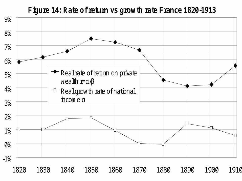
Figure 14: Rate of return vs growth rate France 1820-1913
-1%
0%
1%
2%
3%
4%
5%
6%
7%
8%
9%
1820 1830 1840 1850 1860 1870 1880 1890 1900 1910
Real rate of return on privatewealth r=α/βReal growth rate of nationalincome g
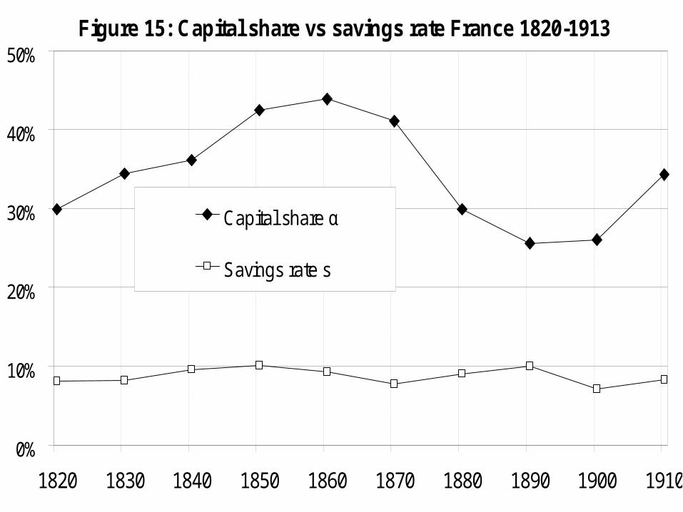
Figure 15: Capital share vs savings rate France 1820-1913
0%
10%
20%
30%
40%
50%
1820 1830 1840 1850 1860 1870 1880 1890 1900 1910
Capital share α
Savings rate s
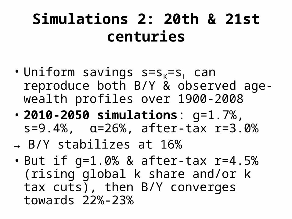
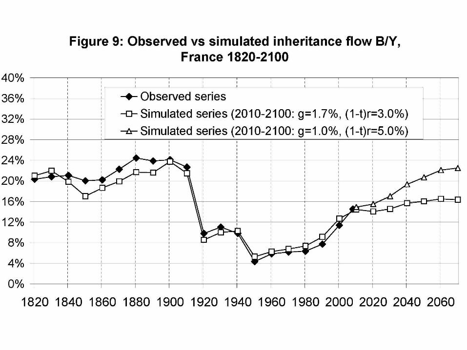
Simulations 2: 20th & 21st centuries
• Uniform savings s=sK=sL can reproduce both B/Y & observed age-wealth profiles over 1900-2008
• 2010-2050 simulations: g=1.7%, s=9.4%, α=26%, after-tax r=3.0%
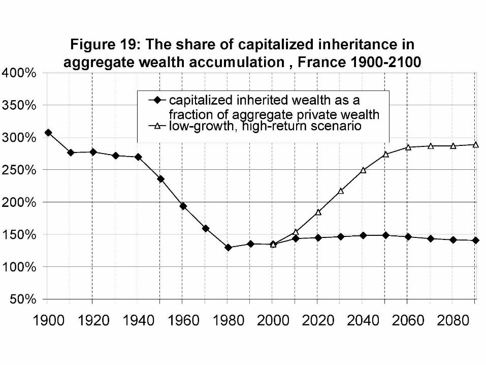
→ B/Y stabilizes at 16%• But if g=1.0% & after-tax r=4.5% (rising
global k share and/or k tax cuts), then B/Y converges towards 22%-23%
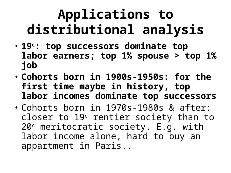
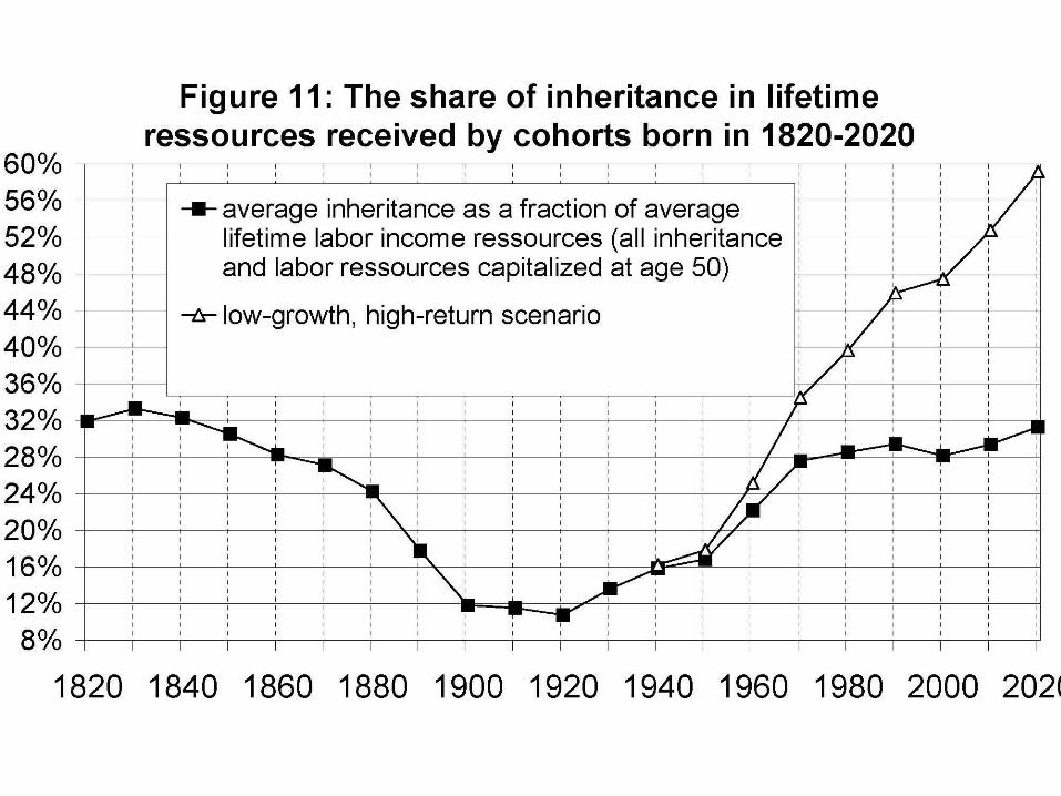
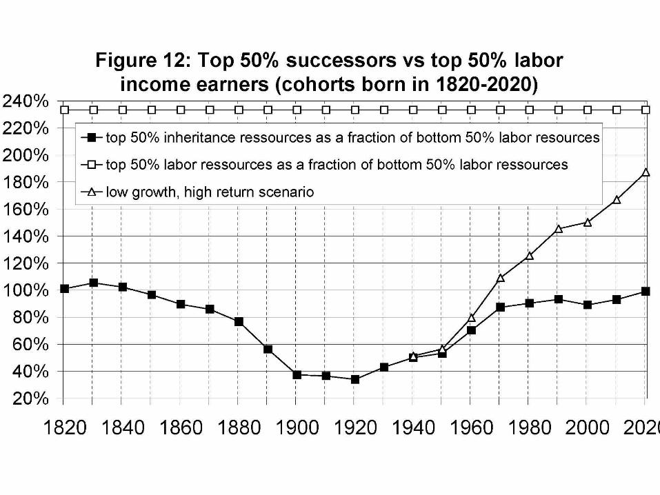
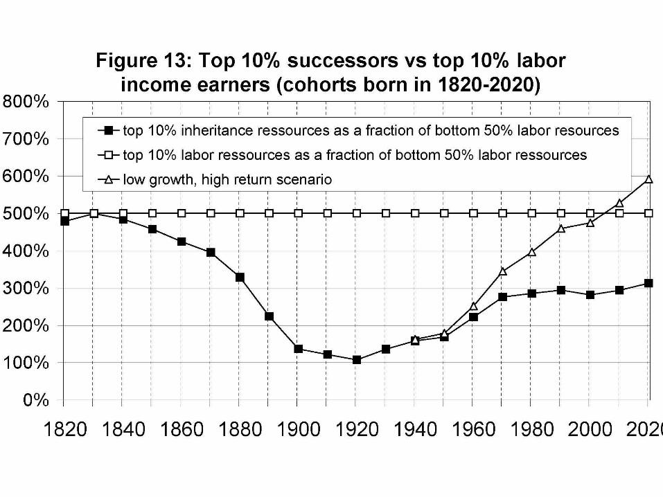
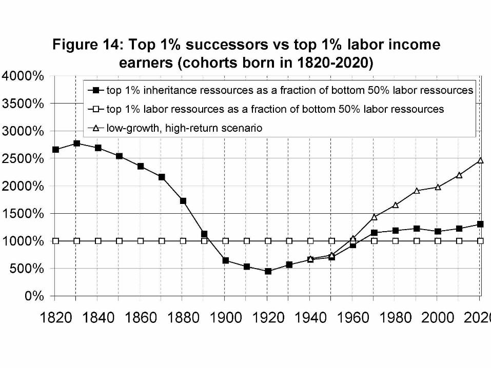
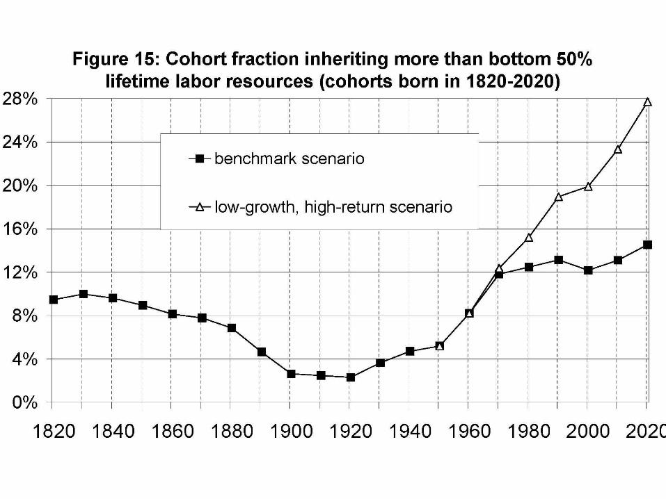
Applications to distributional analysis
• 19c: top successors dominate top labor earners; top 1% spouse > top 1% job
• Cohorts born in 1900s-1950s: for the first time maybe in history, top labor incomes dominate top successors
• Cohorts born in 1970s-1980s & after: closer to 19c rentier society than to 20c meritocratic society. E.g. with labor income alone, hard to buy an appartment in Paris..
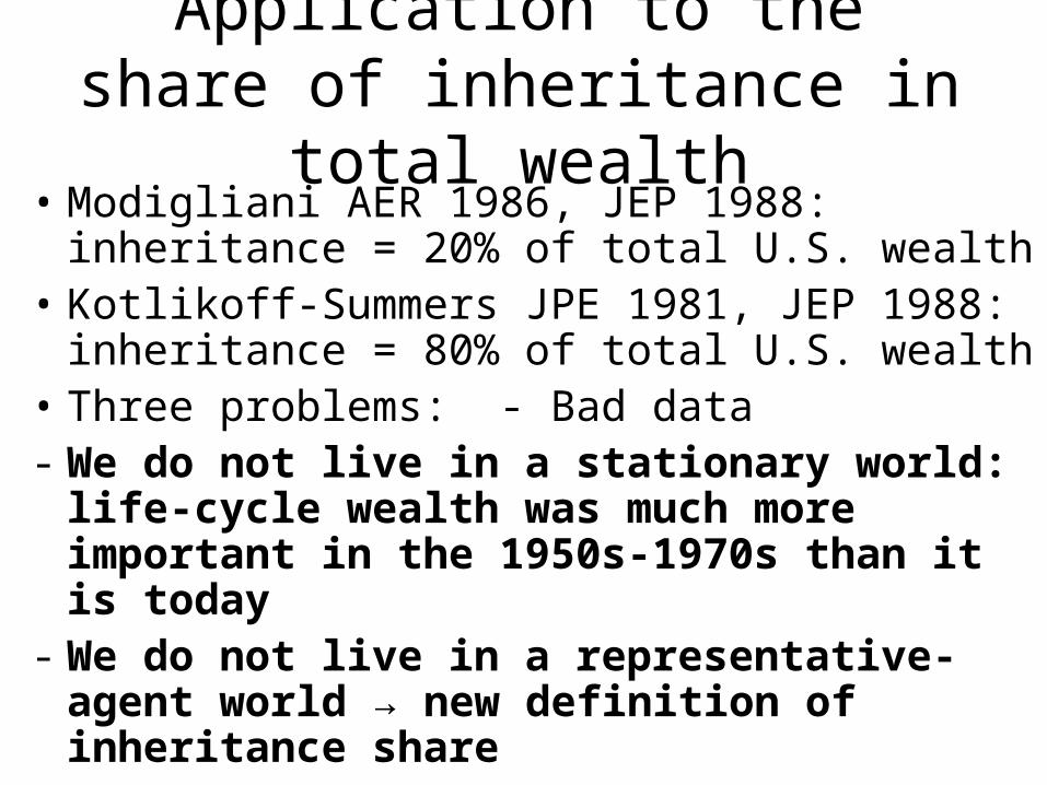
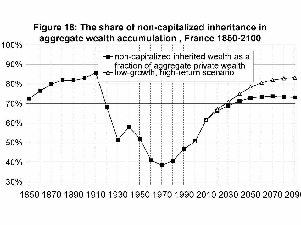
Application to the share of inheritance in total wealth
• Modigliani AER 1986, JEP 1988: inheritance = 20% of total U.S. wealth
• Kotlikoff-Summers JPE 1981, JEP 1988: inheritance = 80% of total U.S. wealth
• Three problems: - Bad data - We do not live in a stationary world: life-
cycle wealth was much more important in the 1950s-1970s than it is today
- We do not live in a representative-agent world → new definition of inheritance share

What have we learned?• Capital accumulation takes time; one
should not look at past 10 or 20 yrs and believe this is steady-state; life cycle theorists were too much influenced by what they saw in the 1950s-1970s…
• Inheritance is likely to be a big issue in the 21st century
• Modern economic growth did not kill inheritance; the rise of human capital simply did not happen; g>0 but small not very different from g=0
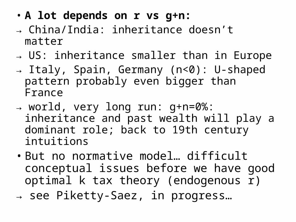
• A lot depends on r vs g+n:→ China/India: inheritance doesn’t matter→ US: inheritance smaller than in Europe→ Italy, Spain, Germany (n<0): U-shaped
pattern probably even bigger than France→ world, very long run: g+n=0%: inheritance
and past wealth will play a dominant role; back to 19th century intuitions
• But no normative model… difficult conceptual issues before we have good optimal k tax theory (endogenous r)
→ see Piketty-Saez, in progress…
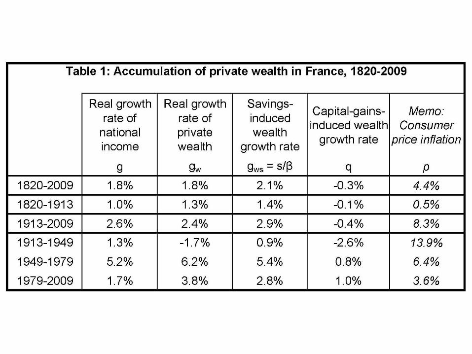
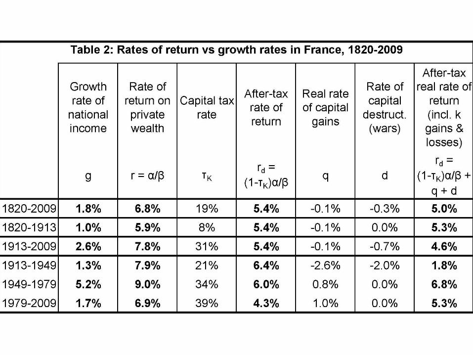
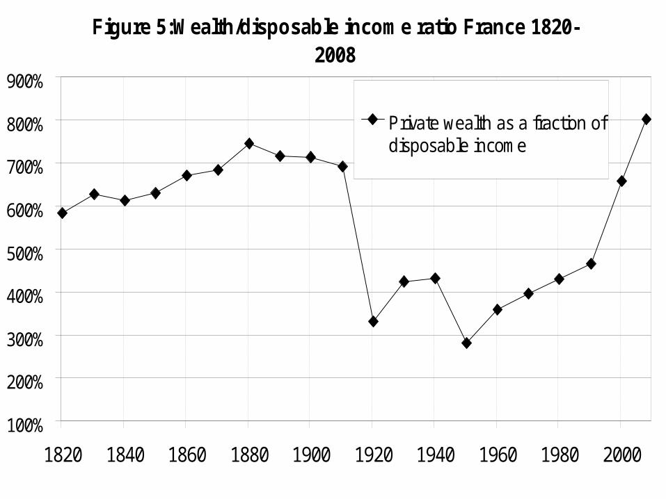
Figure 5:Wealth/disposable income ratio France 1820-2008
100%
200%
300%
400%
500%
600%
700%
800%
900%
1820 1840 1860 1880 1900 1920 1940 1960 1980 2000
Private wealth as a fraction ofdisposable income
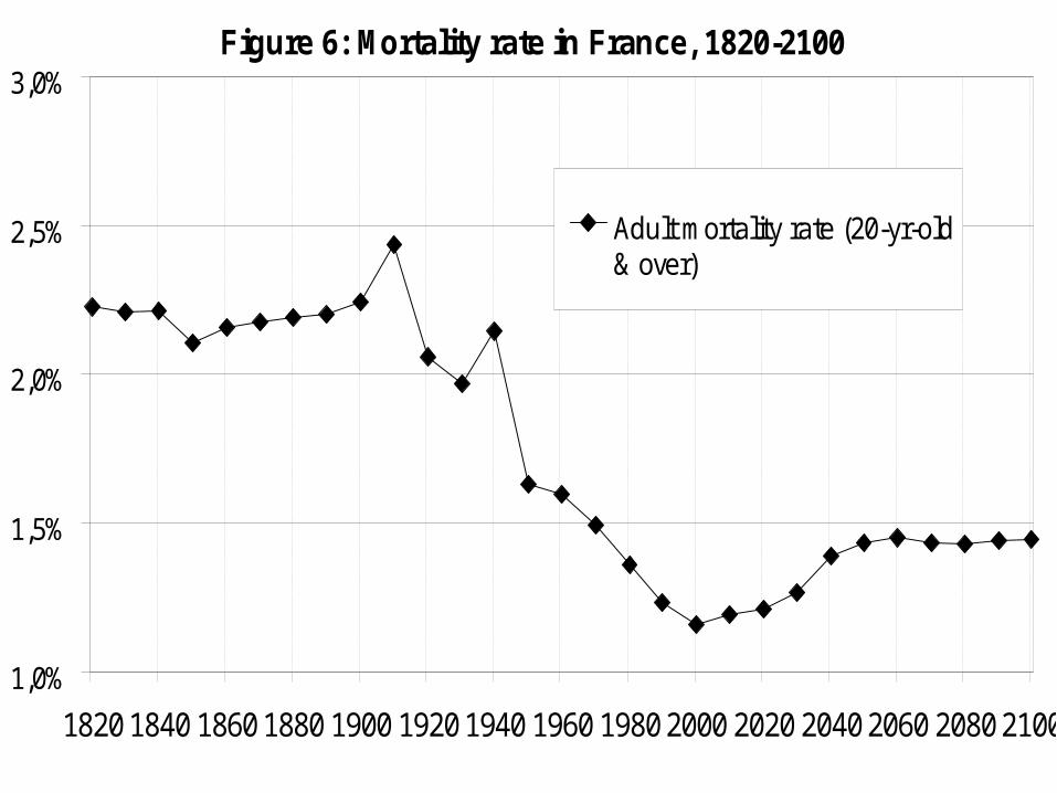
Figure 6: Mortality rate in France, 1820-2100
1,0%
1,5%
2,0%
2,5%
3,0%
1820 1840 1860 1880 1900 1920 1940 1960 1980 2000 2020 2040 2060 2080 2100
Adult mortality rate (20-yr-old& over)
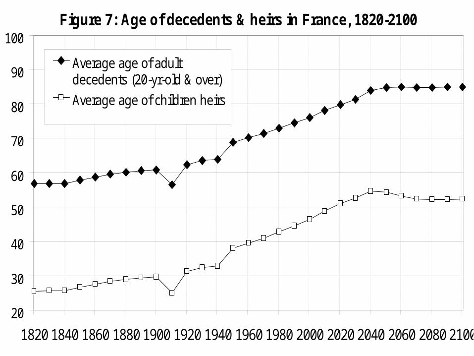
Figure 7: Age of decedents & heirs in France, 1820-2100
20
30
40
50
60
70
80
90
100
1820 1840 1860 1880 1900 1920 1940 1960 1980 2000 2020 2040 2060 2080 2100
Average age of adultdecedents (20-yr-old & over)
Average age of children heirs
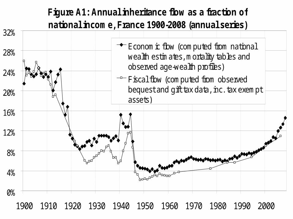
Figure A1: Annual inheritance flow as a fraction of national income, France 1900-2008 (annual series)
0%
4%
8%
12%
16%
20%
24%
28%
32%
1900 1910 1920 1930 1940 1950 1960 1970 1980 1990 2000
Economic flow (computed from nationalwealth estimates, mortality tables andobserved age-wealth profiles)
Fiscal flow (computed from observedbequest and gift tax data, inc. tax exemptassets)
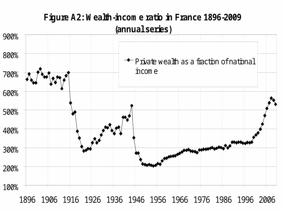
Figure A2: Wealth-income ratio in France 1896-2009 (annual series)
100%
200%
300%
400%
500%
600%
700%
800%
900%
1896 1906 1916 1926 1936 1946 1956 1966 1976 1986 1996 2006
Private wealth as a fraction of nationalincome
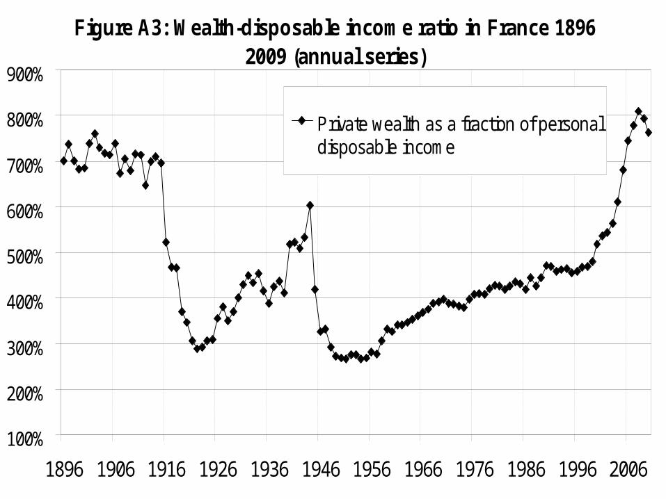
Figure A3: Wealth-disposable income ratio in France 1896-2009 (annual series)
100%
200%
300%
400%
500%
600%
700%
800%
900%
1896 1906 1916 1926 1936 1946 1956 1966 1976 1986 1996 2006
Private wealth as a fraction of personaldisposable income