Discriminatively Trained Sparse Code Gradientsfor Contour Detection

Xiaofeng Ren and Liefeng BoIntel Science and Technology Center for Pervasive Computing, Intel Labs

Seattle, WA 98195, USA{xiaofeng.ren,liefeng.bo}@intel.com

Abstract

Finding contours in natural images is a fundamental problem that serves as thebasis of many tasks such as image segmentation and object recognition. At thecore of contour detection technologies are a set of hand-designed gradient fea-tures, used by most approaches including the state-of-the-art Global Pb (gPb)operator. In this work, we show that contour detection accuracy can be signif-icantly improved by computing Sparse Code Gradients (SCG), which measurecontrast using patch representations automatically learned through sparse coding.We use K-SVD for dictionary learning and Orthogonal Matching Pursuit for com-puting sparse codes on oriented local neighborhoods, and apply multi-scale pool-ing and power transforms before classifying them with linear SVMs. By extract-ing rich representations from pixels and avoiding collapsing them prematurely,Sparse Code Gradients effectively learn how to measure local contrasts and findcontours. We improve the F-measure metric on the BSDS500 benchmark to 0.74(up from 0.71 of gPb contours). Moreover, our learning approach can easily adaptto novel sensor data such as Kinect-style RGB-D cameras: Sparse Code Gradi-ents on depth maps and surface normals lead to promising contour detection usingdepth and depth+color, as verified on the NYU Depth Dataset.

1 IntroductionContour detection is a fundamental problem in vision. Accurately finding both object boundaries andinterior contours has far reaching implications for many vision tasks including segmentation, recog-nition and scene understanding. High-quality image segmentation has increasingly been relying oncontour analysis, such as in the widely used system of Global Pb [2]. Contours and segmentationshave also seen extensive uses in shape matching and object recognition [8, 9].

Accurately finding contours in natural images is a challenging problem and has been extensivelystudied. With the availability of datasets with human-marked groundtruth contours, a variety ofapproaches have been proposed and evaluated (see a summary in [2]), such as learning to clas-sify [17, 20, 16], contour grouping [23, 31, 12], multi-scale features [21, 2], and hierarchical regionanalysis [2]. Most of these approaches have one thing in common [17, 23, 31, 21, 12, 2]: they arebuilt on top of a set of gradient features [17] measuring local contrast of oriented discs, using chi-square distances of histograms of color and textons. Despite various efforts to use generic imagefeatures [5] or learn them [16], these hand-designed gradients are still widely used after a decadeand support top-ranking algorithms on the Berkeley benchmarks [2].

In this work, we demonstrate that contour detection can be vastly improved by replacing the hand-designed Pb gradients of [17] with rich representations that are automatically learned from data.We use sparse coding, in particularly Orthogonal Matching Pursuit [18] and K-SVD [1], to learnsuch representations on patches. Instead of a direct classification of patches [16], the sparse codeson the pixels are pooled over multi-scale half-discs for each orientation, in the spirit of the Pb

1

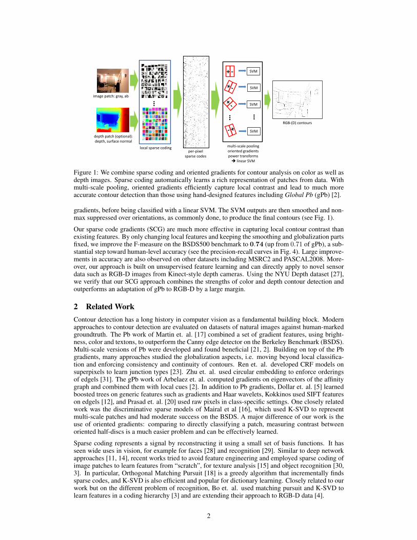
image patch: gray, ab

depth patch (optional): depth, surface normal

…

local sparse coding multi-scale pooling oriented gradients power transforms linear SVM

+ -

…

per-pixel sparse codes

SVM

SVM

SVM

…

SVM

RGB-(D) contours

Figure 1: We combine sparse coding and oriented gradients for contour analysis on color as well asdepth images. Sparse coding automatically learns a rich representation of patches from data. Withmulti-scale pooling, oriented gradients efficiently capture local contrast and lead to much moreaccurate contour detection than those using hand-designed features including Global Pb (gPb) [2].

gradients, before being classified with a linear SVM. The SVM outputs are then smoothed and non-max suppressed over orientations, as commonly done, to produce the final contours (see Fig. 1).

Our sparse code gradients (SCG) are much more effective in capturing local contour contrast thanexisting features. By only changing local features and keeping the smoothing and globalization partsfixed, we improve the F-measure on the BSDS500 benchmark to 0.74 (up from 0.71 of gPb), a sub-stantial step toward human-level accuracy (see the precision-recall curves in Fig. 4). Large improve-ments in accuracy are also observed on other datasets including MSRC2 and PASCAL2008. More-over, our approach is built on unsupervised feature learning and can directly apply to novel sensordata such as RGB-D images from Kinect-style depth cameras. Using the NYU Depth dataset [27],we verify that our SCG approach combines the strengths of color and depth contour detection andoutperforms an adaptation of gPb to RGB-D by a large margin.

2 Related WorkContour detection has a long history in computer vision as a fundamental building block. Modernapproaches to contour detection are evaluated on datasets of natural images against human-markedgroundtruth. The Pb work of Martin et. al. [17] combined a set of gradient features, using bright-ness, color and textons, to outperform the Canny edge detector on the Berkeley Benchmark (BSDS).Multi-scale versions of Pb were developed and found beneficial [21, 2]. Building on top of the Pbgradients, many approaches studied the globalization aspects, i.e. moving beyond local classifica-tion and enforcing consistency and continuity of contours. Ren et. al. developed CRF models onsuperpixels to learn junction types [23]. Zhu et. al. used circular embedding to enforce orderingsof edgels [31]. The gPb work of Arbelaez et. al. computed gradients on eigenvectors of the affinitygraph and combined them with local cues [2]. In addition to Pb gradients, Dollar et. al. [5] learnedboosted trees on generic features such as gradients and Haar wavelets, Kokkinos used SIFT featureson edgels [12], and Prasad et. al. [20] used raw pixels in class-specific settings. One closely relatedwork was the discriminative sparse models of Mairal et al [16], which used K-SVD to representmulti-scale patches and had moderate success on the BSDS. A major difference of our work is theuse of oriented gradients: comparing to directly classifying a patch, measuring contrast betweenoriented half-discs is a much easier problem and can be effectively learned.

Sparse coding represents a signal by reconstructing it using a small set of basis functions. It hasseen wide uses in vision, for example for faces [28] and recognition [29]. Similar to deep networkapproaches [11, 14], recent works tried to avoid feature engineering and employed sparse coding ofimage patches to learn features from “scratch”, for texture analysis [15] and object recognition [30,3]. In particular, Orthogonal Matching Pursuit [18] is a greedy algorithm that incrementally findssparse codes, and K-SVD is also efficient and popular for dictionary learning. Closely related to ourwork but on the different problem of recognition, Bo et. al. used matching pursuit and K-SVD tolearn features in a coding hierarchy [3] and are extending their approach to RGB-D data [4].

2

Thanks to the mass production of Kinect, active RGB-D cameras became affordable and werequickly adopted in vision research and applications. The Kinect pose estimation of Shotton et.al. used random forests to learn from a huge amount of data [25]. Henry et. al. used RGB-D cam-eras to scan large environments into 3D models [10]. RGB-D data were also studied in the contextof object recognition [13] and scene labeling [27, 22]. In-depth studies of contour and segmentationproblems for depth data are much in need given the fast growing interests in RGB-D perception.

3 Contour Detection using Sparse Code GradientsWe start by examining the processing pipeline of Global Pb (gPb) [2], a highly influential andwidely used system for contour detection. The gPb contour detection has two stages: local contrastestimation at multiple scales, and globalization of the local cues using spectral grouping. The coreof the approach lies within its use of local cues in oriented gradients. Originally developed in[17], this set of features use relatively simple pixel representations (histograms of brightness, colorand textons) and similarity functions (chi-square distance, manually chosen), comparing to recentadvances in using rich representations for high-level recognition (e.g. [11, 29, 30, 3]).

We set out to show that both the pixel representation and the aggregation of pixel information in localneighborhoods can be much improved and, to a large extent, learned from and adapted to input data.For pixel representation, in Section 3.1 we show how to use Orthogonal Matching Pursuit [18] andK-SVD [1], efficient sparse coding and dictionary learning algorithms that readily apply to low-levelvision, to extract sparse codes at every pixel. This sparse coding approach can be viewed similarin spirit to the use of filterbanks but avoids manual choices and thus directly applies to the RGB-D data from Kinect. We show learned dictionaries for a number of channels that exhibit differentcharacteristics: grayscale/luminance, chromaticity (ab), depth, and surface normal.

In Section 3.2 we show how the pixel-level sparse codes can be integrated through multi-scale pool-ing into a rich representation of oriented local neighborhoods. By computing oriented gradientson this high dimensional representation and using a double power transform to code the featuresfor linear classification, we show a linear SVM can be efficiently and effectively trained for eachorientation to classify contour vs non-contour, yielding local contrast estimates that are much moreaccurate than the hand-designed features in gPb.

3.1 Local Sparse Representation of RGB-(D) Patches

K-SVD and Orthogonal Matching Pursuit. K-SVD [1] is a popular dictionary learning algorithmthat generalizes K-Means and learns dictionaries of codewords from unsupervised data. Given a setof image patches Y = [y1, · · · , yn], K-SVD jointly finds a dictionary D = [d1, · · · , dm] and anassociated sparse code matrix X = [x1, · · · , xn] by minimizing the reconstruction error

minD,X‖Y −DX‖2F s.t. ∀i, ‖xi‖0 ≤ K; ∀j, ‖dj‖2 = 1 (1)

where ‖ · ‖F denotes the Frobenius norm, xi are the columns of X , the zero-norm ‖ · ‖0 counts thenon-zero entries in the sparse code xi, and K is a predefined sparsity level (number of non-zero en-tries). This optimization can be solved in an alternating manner. Given the dictionary D, optimizingthe sparse code matrixX can be decoupled to sub-problems, each solved with Orthogonal MatchingPursuit (OMP) [18], a greedy algorithm for finding sparse codes. Given the codes X , the dictionaryD and its associated sparse coefficients are updated sequentially by singular value decomposition.For our purpose of representing local patches, the dictionary D has a small size (we use 75 for 5x5patches) and does not require a lot of sample patches, and it can be learned in a matter of minutes.

Once the dictionary D is learned, we again use the Orthogonal Matching Pursuit (OMP) algorithmto compute sparse codes at every pixel. This can be efficiently done with convolution and a batchversion of the OMP algorithm [24]. For a typical BSDS image of resolution 321x481, the sparsecode extraction is efficient and takes 1∼2 seconds.

Sparse Representation of RGB-D Data. One advantage of unsupervised dictionary learning isthat it readily applies to novel sensor data, such as the color and depth frames from a Kinect-styleRGB-D camera. We learn K-SVD dictionaries up to four channels of color and depth: grayscalefor luminance, chromaticity ab for color in the Lab space, depth (distance to camera) and surfacenormal (3-dim). The learned dictionaries are visualized in Fig. 2. These dictionaries are interesting

3

(a) Grayscale (b) Chromaticity (ab) (c) Depth (d) Surface normal

Figure 2: K-SVD dictionaries learned for four different channels: grayscale and chromaticity (inab) for an RGB image (a,b), and depth and surface normal for a depth image (c,d). We use a fixeddictionary size of 75 on 5x5 patches. The ab channel is visualized using a constant luminance of 50.The 3-dimensional surface normal (xyz) is visualized in RGB (i.e. blue for frontal-parallel surfaces).

to look at and qualitatively distinctive: for example, the surface normal codewords tend to be moresmooth due to flat surfaces, the depth codewords are also more smooth but with speckles, and thechromaticity codewords respect the opponent color pairs. The channels are coded separately.

3.2 Coding Multi-Scale Neighborhoods for Measuring Contrast

Multi-Scale Pooling over Oriented Half-Discs. Over decades of research on contour detection andrelated topics, a number of fundamental observations have been made, repeatedly: (1) contrast isthe key to differentiate contour vs non-contour; (2) orientation is important for respecting contourcontinuity; and (3) multi-scale is useful. We do not wish to throw out these principles. Instead, weseek to adopt these principles for our case of high dimensional representations with sparse codes.

Each pixel is presented with sparse codes extracted from a small patch (5-by-5) around it. To aggre-gate pixel information, we use oriented half-discs as used in gPb (see an illustration in Fig. 1). Eachorientation is processed separately. For each orientation, at each pixel p and scale s, we define twohalf-discs (rectangles) Na and N b of size s-by-(2s+1), on both sides of p, rotated to that orienta-tion. For each half-disc N , we use average pooling on non-zero entries (i.e. a hybrid of average andmax pooling) to generate its representation

F (N) =

[∑i∈N|xi1|

/∑i∈N

I|xi1|>0, · · · ,∑i∈N|xim|

/∑i∈N

I|xim|>0

](2)

where xij is the j-th entry of the sparse code xi, and I is the indicator function whether xij is non-zero. We rotate the image (after sparse coding) and use integral images for fast computations (onboth |xij | and |xij | > 0, whose costs are independent of the size of N .

For two oriented half-dics Na and N b at a scale s, we compute a difference (gradient) vector D

D(Nas , N

bs ) =

∣∣F (Nas )− F (N b

s )∣∣ (3)

where | · | is an element-wise absolute value operation. We divide D(Nas , N

bs ) by their norms

‖F (Nas )‖+ ‖F (N b

s )‖+ ε, where ε is a positive number. Since the magnitude of sparse codes variesover a wide range due to local variations in illumination as well as occlusion, this step makes theappearance features robust to such variations and increases their discriminative power, as commonlydone in both contour detection and object recognition. This value is not hard to set, and we find avalue of ε = 0.5 is better than, for instance, ε = 0.

At this stage, one could train a classifier on D for each scale to convert it to a scalar value ofcontrast, which would resemble the chi-square distance function in gPb. Instead, we find that it ismuch better to avoid doing so separately at each scale, but combining multi-scale features in a jointrepresentation, so as to allow interactions both between codewords and between scales. That is, ourfinal representation of the contrast at a pixel p is the concatenation of sparse codes pooled at all the

4

scales s ∈ {1, · · · , S} (we use S = 4):

Dp =[D(Na

1 , Nb1), · · · , D(Na

S , NbS); F (N

a1 ∪N b

1), · · · , F (NaS ∪N b

S)]

(4)

In addition to difference D, we also include a union term F (Nas ∪N b

s ), which captures the appear-ance of the whole disc (union of the two half discs) and is normalized by ‖F (Na

s )‖+ ‖F (N bs )‖+ ε.

Double Power Transform and Linear Classifiers. The concatenated feature Dp (non-negative)provides multi-scale contrast information for classifying whether p is a contour location for a partic-ular orientation. As Dp is high dimensional (1200 and above in our experiments) and we need to doit at every pixel and every orientation, we prefer using linear SVMs for both efficient testing as wellas training. Directly learning a linear function on Dp, however, does not work very well. Instead,we apply a double power transformation to make the features more suitable for linear SVMs

Dp =[Dα1p , Dα2

p

](5)

where 0<α1<α2<1. Empirically, we find that the double power transform works much betterthan either no transform or a single power transform α, as sometimes done in other classificationcontexts. Perronnin et. al. [19] provided an intuition why a power transform helps classification,which “re-normalizes” the distribution of the features into a more Gaussian form. One plausibleintuition for a double power transform is that the optimal exponent α may be different across featuredimensions. By putting two power transforms of Dp together, we allow the classifier to pick itslinear combination, different for each dimension, during the stage of supervised training.

From Local Contrast to Global Contours. We intentionally only change the local contrast es-timation in gPb and keep the other steps fixed. These steps include: (1) the Savitzky-Goley filterto smooth responses and find peak locations; (2) non-max suppression over orientations; and (3)optionally, we apply the globalization step in gPb that computes a spectral gradient from the localgradients and then linearly combines the spectral gradient with the local ones. A sigmoid transformstep is needed to convert the SVM outputs on Dp before computing spectral gradients.

4 ExperimentsWe use the evaluation framework of, and extensively compare to, the publicly available GlobalPb (gPb) system [2], widely used as the state of the art for contour detection1. All the resultsreported on gPb are from running the gPb contour detection and evaluation codes (with defaultparameters), and accuracies are verified against the published results in [2]. The gPb evaluationincludes a number of criteria, including precision-recall (P/R) curves from contour matching (Fig. 4),F-measures computed from P/R (Table 1,2,3) with a fixed contour threshold (ODS) or per-imagethresholds (OIS), as well as average precisions (AP) from the P/R curves.

Benchmark Datasets. The main dataset we use is the BSDS500 benchmark [2], an extension of theoriginal BSDS300 benchmark and commonly used for contour evaluation. It includes 500 naturalimages of roughly resolution 321x481, including 200 for training, 100 for validation, and 200 fortesting. We conduct both color and grayscale experiments (where we convert the BSDS500 imagesto grayscale and retain the groundtruth). In addition, we also use the MSRC2 and PASCAL2008segmentation datasets [26, 6], as done in the gPb work [2]. The MSRC2 dataset has 591 images ofresolution 200x300; we randomly choose half for training and half for testing. The PASCAL2008dataset includes 1023 images in its training and validation sets, roughly of resolution 350x500. Werandomly choose half for training and half for testing.

For RGB-D contour detection, we use the NYU Depth dataset (v2) [27], which includes 1449 pairsof color and depth frames of resolution 480x640, with groundtruth semantic regions. We choose60% images for training and 40% for testing, as in its scene labeling setup. The Kinect images areof lower quality than BSDS, and we resize the frames to 240x320 in our experiments.

Training Sparse Code Gradients. Given sparse codes from K-SVD and Orthogonal Matching Pur-suit, we train the Sparse Code Gradients classifiers, one linear SVM per orientation, from sampledlocations. For positive data, we sample groundtruth contour locations and estimate the orientationsat these locations using groundtruth. For negative data, locations and orientations are random. Wesubtract the mean from the patches in each data channel. For BSDS500, we typically have 1.5 to 2

1In this work we focus on contour detection and do not address how to derive segmentations from contours.

5

2 3 4 5 7 10 140.8

0.82

0.84

0.86

0.88

0.9

pooling disc size (pixel)

aver

age

prec

isio

n

single scaleaccum. scale

25 50 75 100 125 1500.82

0.84

0.86

0.88

0.9

0.92

0.94

dictionary size

aver

age

prec

isio

n

horizontal edge45−deg edgevertical edge135−deg edge

1 2 3 4 5 6 7 80.84

0.86

0.88

0.9

0.92

sparsity level

aver

age

prec

isio

n

graycolor (ab)gray+color

(a) (b) (c)

Figure 3: Analysis of our sparse code gradients, using average precision of classification on sampledboundaries. (a) The effect of single-scale vs multi-scale pooling (accumulated from the smallest).(b) Accuracy increasing with dictionary size, for four orientation channels. (c) The effect of thesparsity level K, which exhibits different behavior for grayscale and chromaticity.

BSDS500ODS OIS AP

loca

l gPb (gray) .67 .69 .68SCG (gray) .69 .71 .71gPb (color) .70 .72 .71SCG (color) .72 .74 .75

glob

al

gPb (gray) .69 .71 .67SCG (gray) .71 .73 .74gPb (color) .71 .74 .72SCG (color) .74 .76 .77

Table 1: F-measure evaluation on the BSDS500benchmark [2], comparing to gPb on grayscaleand color images, both for local contour detec-tion as well as for global detection (i.e. com-bined with the spectral gradient analysis in [2]).

0 0.1 0.2 0.3 0.4 0.5 0.6 0.7 0.8 0.9 10.2

0.3

0.4

0.5

0.6

0.7

0.8

0.9

1

Recall

Pre

cisi

on

gPb (gray) F=0.69gPb (color) F=0.71SCG (gray) F=0.71SCG (color) F=0.74

Figure 4: Precision-recall curves of SCG vsgPb on BSDS500, for grayscale and colorimages. We make a substantial step beyondthe current state of the art toward reachinghuman-level accuracy (green dot).

million data points. We use 4 spatial scales, at half-disc sizes 2, 4, 7, 25. For a dictionary size of 75and 4 scales, the feature length for one data channel is 1200. For full RGB-D data, the dimension is4800. For BSDS500, we train only using the 200 training images. We modify liblinear [7] to takedense matrices (features are dense after pooling) and single-precision floats.

Looking under the Hood. We empirically analyze a number of settings in our Sparse Code Gradi-ents. In particular, we want to understand how the choices in the local sparse coding affect contourclassification. Fig. 3 shows the effects of multi-scale pooling, dictionary size, and sparsity level(K). The numbers reported are intermediate results, namely the mean of average precision of fouroriented gradient classifier (0, 45, 90, 135 degrees) on sampled locations (grayscale unless otherwisenoted, on validation). As a reference, the average precision of gPb on this task is 0.878.

For multi-scale pooling, the single best scale for the half-disc filter is about 4x8, consistent withthe settings in gPb. For accumulated scales (using all the scales from the smallest up to the currentlevel), the accuracy continues to increase and does not seem to be saturated, suggesting the use oflarger scales. The dictionary size has a minor impact, and there is a small (yet observable) benefit touse dictionaries larger than 75, particularly for diagonal orientations (45- and 135-deg). The sparsitylevel K is a more intriguing issue. In Fig. 3(c), we see that for grayscale only, K = 1 (normalizednearest neighbor) does quite well; on the other hand, color needs a larger K, possibly because ab isa nonlinear space. When combining grayscale and color, it seems that we want K to be at least 3. Italso varies with orientation: horizontal and vertical edges require a smaller K than diagonal edges.(If using K = 1, our final F-measure on BSDS500 is 0.730.)

We also empirically evaluate the double power transform vs single power transform vs no transform.With no transform, the average precision is 0.865. With a single power transform, the best choice ofthe exponent is around 0.4, with average precision 0.884. A double power transform (with exponents

6

MSRC2ODS OIS AP

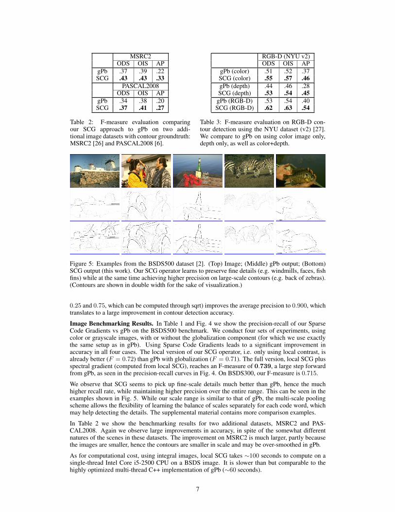
gPb .37 .39 .22SCG .43 .43 .33

PASCAL2008ODS OIS AP

gPb .34 .38 .20SCG .37 .41 .27

Table 2: F-measure evaluation comparingour SCG approach to gPb on two addi-tional image datasets with contour groundtruth:MSRC2 [26] and PASCAL2008 [6].

RGB-D (NYU v2)ODS OIS AP

gPb (color) .51 .52 .37SCG (color) .55 .57 .46gPb (depth) .44 .46 .28SCG (depth) .53 .54 .45

gPb (RGB-D) .53 .54 .40SCG (RGB-D) .62 .63 .54

Table 3: F-measure evaluation on RGB-D con-tour detection using the NYU dataset (v2) [27].We compare to gPb on using color image only,depth only, as well as color+depth.

Figure 5: Examples from the BSDS500 dataset [2]. (Top) Image; (Middle) gPb output; (Bottom)SCG output (this work). Our SCG operator learns to preserve fine details (e.g. windmills, faces, fishfins) while at the same time achieving higher precision on large-scale contours (e.g. back of zebras).(Contours are shown in double width for the sake of visualization.)

0.25 and 0.75, which can be computed through sqrt) improves the average precision to 0.900, whichtranslates to a large improvement in contour detection accuracy.

Image Benchmarking Results. In Table 1 and Fig. 4 we show the precision-recall of our SparseCode Gradients vs gPb on the BSDS500 benchmark. We conduct four sets of experiments, usingcolor or grayscale images, with or without the globalization component (for which we use exactlythe same setup as in gPb). Using Sparse Code Gradients leads to a significant improvement inaccuracy in all four cases. The local version of our SCG operator, i.e. only using local contrast, isalready better (F = 0.72) than gPb with globalization (F = 0.71). The full version, local SCG plusspectral gradient (computed from local SCG), reaches an F-measure of 0.739, a large step forwardfrom gPb, as seen in the precision-recall curves in Fig. 4. On BSDS300, our F-measure is 0.715.

We observe that SCG seems to pick up fine-scale details much better than gPb, hence the muchhigher recall rate, while maintaining higher precision over the entire range. This can be seen in theexamples shown in Fig. 5. While our scale range is similar to that of gPb, the multi-scale poolingscheme allows the flexibility of learning the balance of scales separately for each code word, whichmay help detecting the details. The supplemental material contains more comparison examples.

In Table 2 we show the benchmarking results for two additional datasets, MSRC2 and PAS-CAL2008. Again we observe large improvements in accuracy, in spite of the somewhat differentnatures of the scenes in these datasets. The improvement on MSRC2 is much larger, partly becausethe images are smaller, hence the contours are smaller in scale and may be over-smoothed in gPb.

As for computational cost, using integral images, local SCG takes ∼100 seconds to compute on asingle-thread Intel Core i5-2500 CPU on a BSDS image. It is slower than but comparable to thehighly optimized multi-thread C++ implementation of gPb (∼60 seconds).

7

Figure 6: Examples of RGB-D contour detection on the NYU dataset (v2) [27]. The five panelsare: input image, input depth, image-only contours, depth-only contours, and color+depth contours.Color is good picking up details such as photos on the wall, and depth is useful where color isuniform (e.g. corner of a room, row 1) or illumination is poor (e.g. chair, row 2).

RGB-D Contour Detection. We use the second version of the NYU Depth Dataset [27], whichhas higher quality groundtruth than the first version. A median filtering is applied to remove doublecontours (boundaries from two adjacent regions) within 3 pixels. For RGB-D baseline, we use asimple adaptation of gPb: the depth values are in meters and used directly as a grayscale imagein gPb gradient computation. We use a linear combination to put (soft) color and depth gradientstogether in gPb before non-max suppression, with the weight set from validation.

Table 3 lists the precision-recall evaluations of SCG vs gPb for RGB-D contour detection. Allthe SCG settings (such as scales and dictionary sizes) are kept the same as for BSDS. SCG againoutperforms gPb in all the cases. In particular, we are much better for depth-only contours, forwhich gPb is not designed. Our approach learns the low-level representations of depth data fullyautomatically and does not require any manual tweaking. We also achieve a much larger boost bycombining color and depth, demonstrating that color and depth channels contain complementaryinformation and are both critical for RGB-D contour detection. Qualitatively, it is easy to see thatRGB-D combines the strengths of color and depth and is a promising direction for contour andsegmentation tasks and indoor scene analysis in general [22]. Fig. 6 shows a few examples of RGB-D contours from our SCG operator. There are plenty of such cases where color alone or depth alonewould fail to extract contours for meaningful parts of the scenes, and color+depth would succeed.

5 DiscussionsIn this work we successfully showed how to learn and code local representations to extract contoursin natural images. Our approach combined the proven concept of oriented gradients with powerfulrepresentations that are automatically learned through sparse coding. Sparse Code Gradients (SCG)performed significantly better than hand-designed features that were in use for a decade, and pushedcontour detection much closer to human-level accuracy as illustrated on the BSDS500 benchmark.

Comparing to hand-designed features (e.g. Global Pb [2]), we maintain the high dimensional rep-resentation from pooling oriented neighborhoods and do not collapse them prematurely (such ascomputing chi-square distance at each scale). This passes a richer set of information into learn-ing contour classification, where a double power transform effectively codes the features for linearSVMs. Comparing to previous learning approaches (e.g. discriminative dictionaries in [16]), ouruses of multi-scale pooling and oriented gradients lead to much higher classification accuracies.

Our work opens up future possibilities for learning contour detection and segmentation. As we il-lustrated, there is a lot of information locally that is waiting to be extracted, and a learning approachsuch as sparse coding provides a principled way to do so, where rich representations can be automat-ically constructed and adapted. This is particularly important for novel sensor data such as RGB-D,for which we have less understanding but increasingly more need.

8

References[1] M. Aharon, M. Elad, and A. Bruckstein. K-SVD: An algorithm for designing overcomplete dictionaries

for sparse representation. IEEE Transactions on Signal Processing, 54(11):4311–4322, 2006.[2] P. Arbelaez, M. Maire, C. Fowlkes, and J. Malik. Contour detection and hierarchical image segmentation.

IEEE Trans. PAMI, 33(5):898–916, 2011.[3] L. Bo, X. Ren, and D. Fox. Hierarchical Matching Pursuit for Image Classification: Architecture and Fast

Algorithms. In Advances in Neural Information Processing Systems 24, 2011.[4] L. Bo, X. Ren, and D. Fox. Unsupervised Feature Learning for RGB-D Based Object Recognition. In

International Symposium on Experimental Robotics (ISER), 2012.[5] P. Dollar, Z. Tu, and S. Belongie. Supervised learning of edges and object boundaries. In CVPR, volume 2,

pages 1964–71, 2006.[6] M. Everingham, L. Van Gool, C. K. I. Williams, J. Winn, and A. Zisserman. The PASCAL Visual Object

Classes Challenge 2008 (VOC2008). http://www.pascal-network.org/challenges/VOC/voc2008/.[7] R. Fan, K. Chang, C. Hsieh, X. Wang, and C. Lin. Liblinear: A library for large linear classification. The

Journal of Machine Learning Research, 9:1871–1874, 2008.[8] V. Ferrari, T. Tuytelaars, and L. V. Gool. Object detection by contour segment networks. In ECCV, pages

14–28, 2006.[9] C. Gu, J. Lim, P. Arbelaez, and J. Malik. Recognition using regions. In CVPR, pages 1030–1037, 2009.

[10] P. Henry, M. Krainin, E. Herbst, X. Ren, and D. Fox. Rgb-d mapping: Using depth cameras for dense 3dmodeling of indoor environments. In International Symposium on Experimental Robotics (ISER), 2010.

[11] G. Hinton, S. Osindero, and Y. Teh. A fast learning algorithm for deep belief nets. Neural computation,18(7):1527–1554, 2006.

[12] I. Kokkinos. Highly accurate boundary detection and grouping. In CVPR, pages 2520–2527, 2010.[13] K. Lai, L. Bo, X. Ren, and D. Fox. A large-scale hierarchical multi-view RGB-D object dataset. In ICRA,

pages 1817–1824, 2011.[14] H. Lee, R. Grosse, R. Ranganath, and A. Ng. Convolutional deep belief networks for scalable unsuper-

vised learning of hierarchical representations. In ICML, pages 609–616, 2009.[15] J. Mairal, F. Bach, J. Ponce, G. Sapiro, and A. Zisserman. Discriminative learned dictionaries for local

image analysis. In CVPR, pages 1–8, 2008.[16] J. Mairal, M. Leordeanu, F. Bach, M. Hebert, and J. Ponce. Discriminative sparse image models for

class-specific edge detection and image interpretation. ECCV, pages 43–56, 2008.[17] D. Martin, C. Fowlkes, and J. Malik. Learning to detect natural image boundaries using brightness and

texture. In Advances in Neural Information Processing Systems 15, 2002.[18] Y. Pati, R. Rezaiifar, and P. Krishnaprasad. Orthogonal Matching Pursuit: Recursive Function Approx-

imation with Applications to Wavelet Decomposition. In The Twenty-Seventh Asilomar Conference onSignals, Systems and Computers, pages 40–44, 1993.

[19] F. Perronnin, J. Sanchez, and T. Mensink. Improving the fisher kernel for large-scale image classification.In ECCV, pages 143–156, 2010.

[20] M. Prasad, A. Zisserman, A. Fitzgibbon, M. Kumar, and P. Torr. Learning class-specific edges for objectdetection and segmentation. Computer Vision, Graphics and Image Processing, pages 94–105, 2006.

[21] X. Ren. Multi-scale improves boundary detection in natural images. In ECCV, pages 533–545, 2008.[22] X. Ren, L. Bo, and D. Fox. RGB-(D) scene labeling: features and algorithms. In Computer Vision and

Pattern Recognition (CVPR), 2012 IEEE Conference on, pages 2759–2766. IEEE, 2012.[23] X. Ren, C. Fowlkes, and J. Malik. Cue integration in figure/ground labeling. In Advances in Neural

Information Processing Systems 18, 2005.[24] R. Rubinstein, M. Zibulevsky, and M. Elad. Efficient Implementation of the K-SVD Algorithm using

Batch Orthogonal Matching Pursuit. Technical report, CS Technion, 2008.[25] J. Shotton, A. Fitzgibbon, M. Cook, T. Sharp, M. Finocchio, R. Moore, A. Kipman, and A. Blake. Real-

time human pose recognition in parts from single depth images. In CVPR, volume 2, page 3, 2011.[26] J. Shotton, J. Winn, C. Rother, and A. Criminisi. Textonboost: Joint appearance, shape and context

modeling for multi-class object recognition and segmentation. In ECCV, 2006.[27] N. Silberman and R. Fergus. Indoor scene segmentation using a structured light sensor. In IEEE Workshop

on 3D Representation and Recognition (3dRR), 2011.[28] J. Wright, A. Yang, A. Ganesh, S. Sastry, and Y. Ma. Robust face recognition via sparse representation.

IEEE Trans. PAMI, 31(2):210–227, 2009.[29] J. Yang, K. Yu, Y. Gong, and T. Huang. Linear spatial pyramid matching using sparse coding for image

classification. In CVPR, pages 1794–1801, 2009.[30] K. Yu, Y. Lin, and J. Lafferty. Learning image representations from the pixel level via hierarchical sparse

coding. In CVPR, pages 1713–1720, 2011.[31] Q. Zhu, G. Song, and J. Shi. Untangling cycles for contour grouping. In ICCV, 2007.

9