Discriminating Clear-sky from Clouds with MODIS

STEVEN A. ACKERMAN, KATHLEEN I. STRABALA, W. PAUL MENZEL,

RICHARD A. FREY, CHRISTOPHER C. MOELLER, AND LIAM E. GUMLEY

Journal of Geophysical Research

(Manuscript submitted 28 November 1997)

Abstract

The MODIS cloud mask uses several cloud detection tests to indicate a level of

confidence that the MODIS is observing clear skies. It will be produced globally at single pixel

resolution; the algorithm uses as many as fourteen of the MODIS 36 spectral bands to maximize

reliable cloud detection and to mitigate past difficulties experienced by sensors with coarser

spatial resolution or fewer spectral bands. The MODIS cloud mask is ancillary input to MODIS

land, ocean and atmosphere science algorithms to suggest processing options. The MODIS cloud

mask algorithm will operate in near-real time in a limited computer processing and storage facility

with simple easy to follow algorithm paths.

The MODIS cloud mask algorithm identifies several conceptual domains according to

surface type and solar illumination including land, water, snow/ice, desert, and coast for both day

and night. Once a pixel has been assigned to a particular domain (defining an algorithm path), a

series of threshold tests attempts to detect the presence of clouds in the instrument field-of-view.

Each cloud detection test returns a confidence level that the pixel is clear ranging in value from 1

(high) to 0 (low). There are several types of tests, where detection of different cloud conditions

relies on different tests. Tests capable of detecting similar cloud conditions are grouped together.

While these groups are arranged so that independence between them is maximized, few, if any,

spectral tests are completely independent. The minimum confidence from all tests within a group

2

is taken to be representative of that group. These confidences indicate absence of particular cloud

types. The product of all the group confidences is used to determine the confidence of finding

clear-sky conditions.

This paper outlines the MODIS cloud masking algorithm. While no present sensor has all

of the spectral bands necessary for testing the complete MODIS cloud mask, initial validation of

some of the individual cloud tests is presented using existing remote sensing data sets.

3

1.0 Introduction

The MODerate resolution Imaging Spectroradiometer (MODIS) is a keystone instrument

of the Earth Observing System (EOS) for conducting global change research. The MODIS

provides global observations of earth’s land, oceans, and atmosphere in the visible and infrared

regions of the spectrum. Measurements at 36 wavelengths, from 0.4 to 14.5 µm, will allow

investigators to study the earth in unprecedented detail. Biological and geophysical processes will

be recorded in the MODIS measurements on a global scale every 1 to 2 days. Many of the

atmospheric and surface parameters require cloud free measurements. The MODIS cloud mask

provides an estimate that a given MODIS field of view (FOV) is cloud free. It is a global Level 2

product generated daily at 1 km and 250 m spatial resolutions.

MODIS measures radiances in two visible bands at 250 m spatial resolution, five more

visible bands at 500 m resolution, and the remaining 29 visible and infrared bands at 1000 m

resolution. Radiances from 14 spectral bands (Table 1) are used in the MODIS cloud mask

algorithm to estimate whether a given view of the earth surface is unobstructed by clouds or

optically thick aerosol, and whether a clear scene is affected by cloud shadows.

The operational processing of MODIS requires adequate CPU capability, large file sizes,

and easy comprehension of the output cloud masks. A note on each of these concerns follows.

◊ The cloud mask algorithm lies at the beginning of the data processing chain for most MODIS

products and thus must run in near-real time, limiting the use of CPU-intensive algorithms.

◊ Storage requirements are a concern. The cloud mask is more than a yes/no decision. The

cloud mask consists of 48 bits of output that include information on individual cloud test

results, the processing path, and ancillary information (e.g., land/sea tag). The first 8 bits of

the cloud mask provide a summary adequate for many processing applications; however, some

applications will require the full mask at 4.8 Gigabytes of storage per day.

◊ The cloud mask must be easily understood but provide enough information for wide use; it

must be simple in concept but effective in its application.

This paper describes the approach for detecting clouds using MODIS observations and

details the algorithms. Section 2 presents a very brief summary of some current global cloud

detection algorithms and discusses the wavelengths used in the MODIS cloud mask algorithm.

Section 3 discusses the approach employed by the algorithm. Section 4 details the input and

4

outputs of the algorithm. Section 5 describes some attempts at validation using current aircraft

and space-borne sensors. Section 6 provides examples on how to interpret the cloud mask

results. A summary is given in Section 7.

5

2.0 Background

The MODIS cloud mask algorithm benefits from several previous efforts to characterize

global cloud cover using satellite observations. The International Satellite Cloud Climatology

Project (ISCCP) [Rossow 1989; Rossow et al. 1993; Seze and Rossow 1991; Rossow and Gardner

1993a, 1993b] has developed cloud detection schemes using visible and infrared window

radiances. The AVHRR (Advanced Very High Resolution Radiometer) Processing scheme Over

cLoud Land and Ocean (APOLLO) [Saunders and Kriebel 1988; Kriebel and Saunders 1988;

Gesell 1989] uses the two visible and three infrared bands of the AVHRR. The NOAA CLoud

Advanced Very high resolution Radiometer (CLAVR) [Stowe et al. 1991; Stowe et al. 1994] adds

a series of spectral and spatial variability tests to detect cloud. CO2 Slicing [Wylie et al. 1994]

characterizes global high cloud cover, including thin cirrus, using radiances in the carbon dioxide

sensitive portion of the spectrum. Frey et al. [1995] developed a real-time, global algorithm for

detecting cloud using collocated AVHRR and High resolution Infrared Radiation Sounder

(HIRS/2) observations. Many other algorithms have been developed for cloud clearing using the

TIROS-N Operational Vertical Sounder (TOVS); Smith et al. [1993] use collocated AVHRR and

HIRS/2 to cloud clear, while Rizzi et al. [1994] base their work on the N* approach developed by

Smith [1968].

These algorithms have been used in global cloud climatologies over long time periods and

thus have overcome some of the difficulties facing the MODIS cloud mask algorithm. A wide

variety of scientists have discussed the physical basis behind each of the MODIS spectral tests and

applications to satellite or aircraft data are present in a variety of publications (Ackerman et al.

[1997] include a reference list). The MODIS cloud mask algorithm builds on these past works by

combining the different tests into a single unified algorithm at high spatial resolution.

The following notation is used in this paper: satellite measured solar reflectance is r, and

brightness temperature (equivalent blackbody temperature from the Planck radiance) is BT.

6

3.0 Algorithm

Clouds are generally characterized by higher reflectance and lower temperature than the

underlying earth surface. Simple visible and infrared window threshold approaches offer

considerable skill in cloud detection; however, many surface conditions reduce cloud-surface

contrast in certain spectral regions, (e.g. bright clouds over snow and ice). Cloud types such as

thin cirrus, low level stratus at night, and small cumulus typically have low contrast with the

underlying background. Cloud edges cause further difficulty since the instrument field of view will

not always be completely cloudy or clear. The 36 spectral bands on the MODIS offer the

opportunity for multispectral approaches to global cloud detection whereby many of these

concerns can be mitigated.

Differences in the cloud-surface contrast across the spectrum can make a pixel appear

cloudy in one spectral band and cloud free in another. To illustrate this point, Figure 1 presents

three spectral images (histogram normalized) of a sub-visual contrail taken from the MODIS

Airborne Simulator (MAS) during the Subsonic Aircraft Contrail and Cloud Effects Special Study

(SUCCESS.) The left panel shows a MAS visible image at 0.66 µm, a spectral region found on

many satellite sensors and commonly used by land surface classifications such as the vegetation

index. The contrail is not apparent in this image. The right panel shows a MAS infrared window

image at 11 µm (dark is cold, light is warm), again a spectral region found on many satellite

sensors and commonly used to infer surface temperatures. There is very modest indication of a

contrail, but it would be difficult to fully define its extent. The center panel shows the MAS 1.88

µm spectral band which is located near a strong water vapor absorption band and is extremely

sensitive to the presence of high level clouds in daylight. The full contrail is very apparent. While

the contrail seems to have little impact on visible reflectances, its effect is likely to be sufficient in

the infrared window to affect estimates of surface temperature. In this type of scene, the cloud

mask needs to provide information useful in both visible (no impact of contrail) and infrared

(likely impact of contrail) applications. The 1.88 µm spectral band on MAS is expected to exhibit

similar characteristics to the 1.38 µm spectral band to be available on MODIS, both are near a

strong water vapor absorption band.

7

The MODIS cloud mask algorithm determines if a given pixel is clear by combining the

results of several spectral threshold tests. All of the spectral cloud detection tests described below

rely on thresholds. Thresholds are never global. There are always exceptions and the thresholds

need to be interpreted carefully. For example, if the visible reflectance over the ocean (away from

sunglint) is greater than 6% then the pixel is often identified as cloudy. However, it seems

unrealistic to label a pixel with a reflectance of 6.1 as cloudy, and a neighboring pixel with the

reflectance of 6.0 as non-cloudy. Rather, as one approaches the threshold limit, the certainty or

confidence in the cloud detection becomes less certain. Individual confidence values are assigned

to the single pixel tests and a final determination of whether the pixel is clear or cloudy is forged

from the product of the individual confidence values.

Application of the individual spectral tests results in a confidence in the clear or cloudy

determination for each FOV. Each test is assigned a value between 0 and 1 where 0 represents

high confidence in cloudy conditions and 1 represents high confidence in clear conditions and the

numbers in between represent increasingly less confidence in cloudy or clear conditions as 0.5 is

approached. Figure 2 is a graphical representation of how a confidence level is assigned for a

given spectral test. The abscissa represents the observation and the ordinate the clear-sky

confidence level. In this test, an observation greater than a value of γ is determined to be a high

confidence clear scene and assigned a value of 1. An observation with a value less than α is

cloudy and assigned a confidence level of 0. These high confidence clear and cloud thresholds, γ

and α respectively, are determined from previous studies, observations, and/or theoretical

simulations. Observations between α and γ are assigned a confidence value between 0 and 1 based

on a linear function.

The MODIS cloud mask output includes the results from each individual test in binary

form; either cloud (denoted by 0) or clear (denoted by 1) without the confidence in this particular

test (denoted by values between 0 and 1). This enables a user to inspect the results of a particular

test and also allows the algorithm developer to track possible causes of cloud mask problems as

they occur. The β value in Figure 2 is the pass/fail threshold for a test. Each test therefore has

threshold values for pass/fail, high confidence pass and high confidence fail. Some tests, such as

the visible ratio test, identify cloud if the observations fall within a given range (e.g., 0.9 < r0.87/

8

r0.66 < 1.1); for such a test there are three thresholds for each end of the range, six thresholds in

all.

The uncertainty inherent in a threshold test is caused by instrument noise, inadequate

characterization of the radiative properties of the earth surface, and variations in atmospheric

emission and scattering. The initial determination of cloud or clear within a MODIS FOV is an

amalgamation of the confidence values for all the single pixel tests. This initial determination

dictates whether additional testing (e.g., spatial uniformity tests) is warranted to improve the

confidence. The final determination assigns one of four levels: confident clear, probably clear,

undecided, and cloudy. This approach attempts to quantify the confidence in the derived cloud

mask for a given pixel. Thus, the MODIS cloud mask algorithm produces more than a yes/no

decision.

As discussed earlier, a variety of spectral observations enhance the chance of determining

the presence of a cloud (e.g. Figure 1). The spectral tests in one spectral region can compensate

for the problems with spectral tests in another spectral region. In the MODIS cloud mask

algorithm each spectral test is placed in one of five groups: (1) detecting thick high clouds with

emitted radiation threshold tests using the brightness temperatures of BT11, BT13.9, and BT6.7; (2)

detecting thin clouds with brightness temperature difference tests BT11- BT12, BT8.6 - BT11, BT11-

BT3.9, and, BT11- BT6.7; (3) detecting low clouds with reflectance thresholds for r0.87, r0.65, and

r.936, reflectance ratio tests, and a brightness temperature difference test BT3.9- BT3.7; (4) detecting

upper tropospheric thin clouds with a reflectance threshold test for r1.38 ; and (5) cirrus sensitive

brightness temperature difference tests BT11- BT12, BT12- BT4, and BT13.7- BT13.9. Tests within a

group may detect more than one cloud type. Thresholds for each test can be found in the MODIS

cloud mask Algorithm Theoretical Basis Document [Ackerman et al. 1997].

Consider the example of daytime stratocumulus and cirrus clouds over oceans in regions

without sun glint. Stratocumulus clouds will likely be detected by the visible reflectance test, the

reflectance ratio test, and the BT11-BT3.7. Very thin cirrus clouds would best be detected by the

1.38 µm and BT11- BT12 APOLLO tests, two tests which have difficulty detecting low level

clouds. It is important to realize that the cloud mask tests in the different groups are not

independent of one another. The task is to combine the different spectral cloud detection tests in

the most effective manner. Several different methods of combining the individual tests have been

9

investigated using a variety of data sets (see Section 5). The technique described below produced

consistent cloud detection.

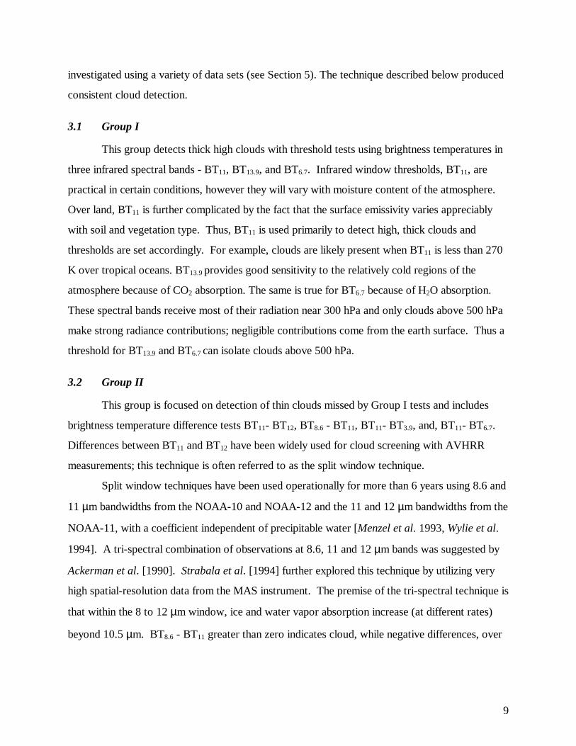
3.1 Group I

This group detects thick high clouds with threshold tests using brightness temperatures in

three infrared spectral bands - BT11, BT13.9, and BT6.7. Infrared window thresholds, BT11, are

practical in certain conditions, however they will vary with moisture content of the atmosphere.

Over land, BT11 is further complicated by the fact that the surface emissivity varies appreciably

with soil and vegetation type. Thus, BT11 is used primarily to detect high, thick clouds and

thresholds are set accordingly. For example, clouds are likely present when BT11 is less than 270

K over tropical oceans. BT13.9 provides good sensitivity to the relatively cold regions of the

atmosphere because of CO2 absorption. The same is true for BT6.7 because of H2O absorption.

These spectral bands receive most of their radiation near 300 hPa and only clouds above 500 hPa

make strong radiance contributions; negligible contributions come from the earth surface. Thus a

threshold for BT13.9 and BT6.7 can isolate clouds above 500 hPa.

3.2 Group II

This group is focused on detection of thin clouds missed by Group I tests and includes

brightness temperature difference tests BT11- BT12, BT8.6 - BT11, BT11- BT3.9, and, BT11- BT6.7.

Differences between BT11 and BT12 have been widely used for cloud screening with AVHRR

measurements; this technique is often referred to as the split window technique.

Split window techniques have been used operationally for more than 6 years using 8.6 and

11 µm bandwidths from the NOAA-10 and NOAA-12 and the 11 and 12 µm bandwidths from the

NOAA-11, with a coefficient independent of precipitable water [Menzel et al. 1993, Wylie et al.

1994]. A tri-spectral combination of observations at 8.6, 11 and 12 µm bands was suggested by

Ackerman et al. [1990]. Strabala et al. [1994] further explored this technique by utilizing very

high spatial-resolution data from the MAS instrument. The premise of the tri-spectral technique is

that within the 8 to 12 µm window, ice and water vapor absorption increase (at different rates)

beyond 10.5 µm. BT8.6 - BT11 greater than zero indicates cloud, while negative differences, over

10

oceans, indicate clear regions. As atmospheric moisture increases, BT8.6 - BT11 decreases while

BT11 - BT12 increases.

Brightness temperature difference techniques using MODIS will be very sensitive to thin

clouds if the surface emissivity and temperature are adequately characterized. For example, given

a surface at 300 K and a cloud at 220 K, a cloud emissivity of .01 affects the sensed infrared

window brightness temperature by .5 K. Since the anticipated noise equivalent temperature for

many of the MODIS infrared window spectral bands is better than .05 K, the cloud detection

capability will obviously be very good.

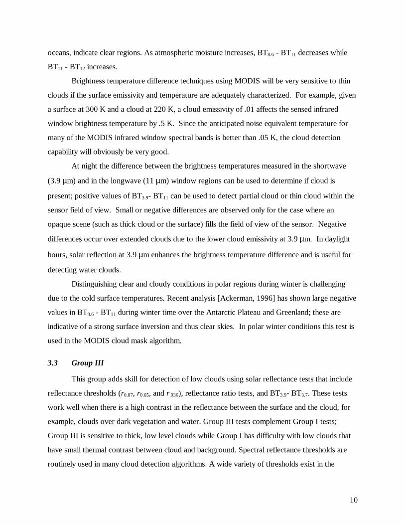
At night the difference between the brightness temperatures measured in the shortwave

(3.9 µm) and in the longwave (11 µm) window regions can be used to determine if cloud is

present; positive values of BT3.9- BT11 can be used to detect partial cloud or thin cloud within the

sensor field of view. Small or negative differences are observed only for the case where an

opaque scene (such as thick cloud or the surface) fills the field of view of the sensor. Negative

differences occur over extended clouds due to the lower cloud emissivity at 3.9 µm. In daylight

hours, solar reflection at 3.9 µm enhances the brightness temperature difference and is useful for

detecting water clouds.

Distinguishing clear and cloudy conditions in polar regions during winter is challenging

due to the cold surface temperatures. Recent analysis [Ackerman, 1996] has shown large negative

values in BT8.6 - BT11 during winter time over the Antarctic Plateau and Greenland; these are

indicative of a strong surface inversion and thus clear skies. In polar winter conditions this test is

used in the MODIS cloud mask algorithm.

3.3 Group III

This group adds skill for detection of low clouds using solar reflectance tests that include

reflectance thresholds (r0.87, r0.65, and r.936), reflectance ratio tests, and BT3.9- BT3.7. These tests

work well when there is a high contrast in the reflectance between the surface and the cloud, for

example, clouds over dark vegetation and water. Group III tests complement Group I tests;

Group III is sensitive to thick, low level clouds while Group I has difficulty with low clouds that

have small thermal contrast between cloud and background. Spectral reflectance thresholds are

routinely used in many cloud detection algorithms. A wide variety of thresholds exist in the

11

literature, depending on surface type and solar and view angle geometry. The initial MODIS

thresholds are given in Ackerman et al. 1997. These thresholds are selected based on previous

studies and data analyses described in Section 5. It is likely that these thresholds will be slightly

adjusted post-launch.

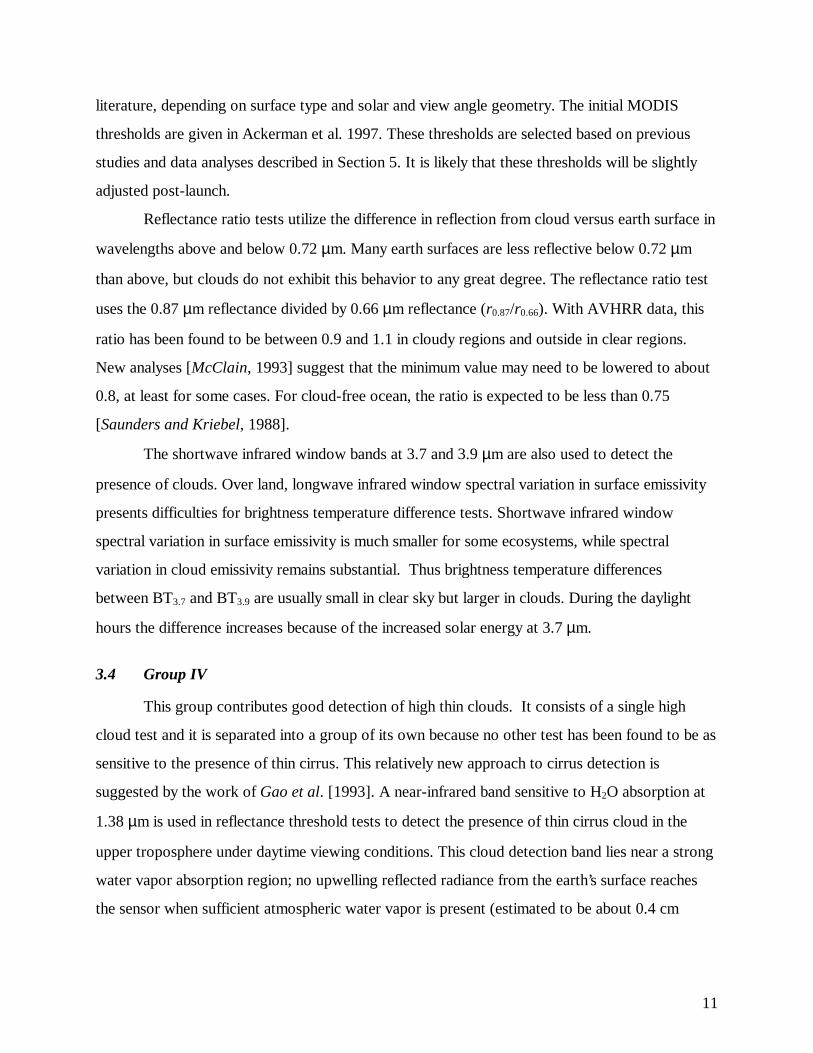
Reflectance ratio tests utilize the difference in reflection from cloud versus earth surface in

wavelengths above and below 0.72 µm. Many earth surfaces are less reflective below 0.72 µm

than above, but clouds do not exhibit this behavior to any great degree. The reflectance ratio test

uses the 0.87 µm reflectance divided by 0.66 µm reflectance (r0.87/r0.66). With AVHRR data, this

ratio has been found to be between 0.9 and 1.1 in cloudy regions and outside in clear regions.

New analyses [McClain, 1993] suggest that the minimum value may need to be lowered to about

0.8, at least for some cases. For cloud-free ocean, the ratio is expected to be less than 0.75

[Saunders and Kriebel, 1988].

The shortwave infrared window bands at 3.7 and 3.9 µm are also used to detect the

presence of clouds. Over land, longwave infrared window spectral variation in surface emissivity

presents difficulties for brightness temperature difference tests. Shortwave infrared window

spectral variation in surface emissivity is much smaller for some ecosystems, while spectral

variation in cloud emissivity remains substantial. Thus brightness temperature differences

between BT3.7 and BT3.9 are usually small in clear sky but larger in clouds. During the daylight

hours the difference increases because of the increased solar energy at 3.7 µm.

3.4 Group IV

This group contributes good detection of high thin clouds. It consists of a single high

cloud test and it is separated into a group of its own because no other test has been found to be as

sensitive to the presence of thin cirrus. This relatively new approach to cirrus detection is

suggested by the work of Gao et al. [1993]. A near-infrared band sensitive to H2O absorption at

1.38 µm is used in reflectance threshold tests to detect the presence of thin cirrus cloud in the

upper troposphere under daytime viewing conditions. This cloud detection band lies near a strong

water vapor absorption region; no upwelling reflected radiance from the earth’s surface reaches

the sensor when sufficient atmospheric water vapor is present (estimated to be about 0.4 cm

12

precipitable water) in the FOV. Simple low and high reflectance thresholds can be used to

separate thin cirrus from clear and thick (near-infrared cloud optical depth > ∼ 0.2) cloud scenes.

3.5 Group V

Group V cloud detection tests also focus on detection of high thin cirrus. Group V tests

consist of brightness temperature difference tests BT11- BT12, BT12- BT4, and BT13.7- BT13.9. The

Group V tests are similar to those in Group II, but they are specially tuned to detect the presence

of thin cirrus. BT11- BT12 is greater than zero in ice clouds due to the larger absorption at the

longer wavelength in the infrared window. BT12- BT4 is less than zero in semitransparent cirrus as

subpixel warm features dominate the shortwave window radiances within a FOV. BT13.7- BT13.9 is

nominally positive in clear skies, but goes to zero when viewing cirrus. The large differences

between ground and cloud temperatures make these tests useful for thin cirrus detection.

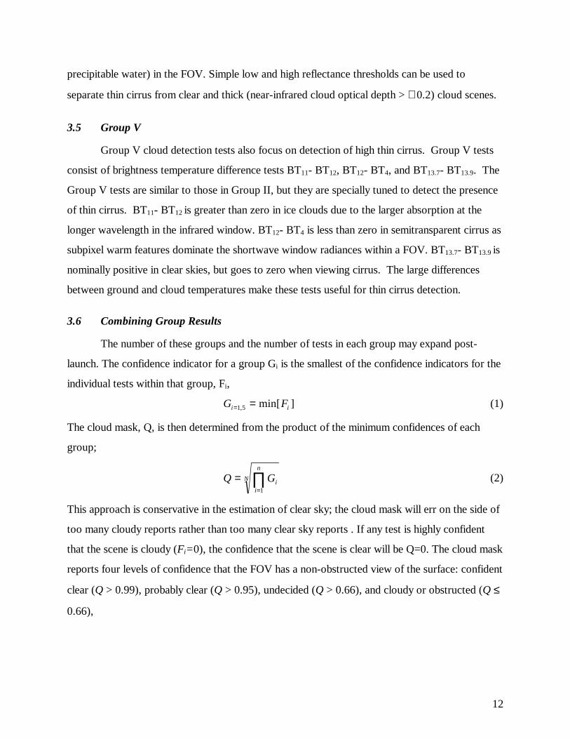
3.6 Combining Group Results

The number of these groups and the number of tests in each group may expand post-

launch. The confidence indicator for a group Gi is the smallest of the confidence indicators for the

individual tests within that group, Fi,

G Fi i= =1 5, min[ ] (1)

The cloud mask, Q, is then determined from the product of the minimum confidences of each

group;

Q Gii

n

N==

∏1

(2)

This approach is conservative in the estimation of clear sky; the cloud mask will err on the side of

too many cloudy reports rather than too many clear sky reports . If any test is highly confident

that the scene is cloudy (Fi=0), the confidence that the scene is clear will be Q=0. The cloud mask

reports four levels of confidence that the FOV has a non-obstructed view of the surface: confident

clear (Q > 0.99), probably clear (Q > 0.95), undecided (Q > 0.66), and cloudy or obstructed (Q ≤

0.66),

13

4.0 Cloud Mask Inputs and Outputs

This section summarizes the input and output of the MODIS cloud mask algorithm. As

indicated earlier, the cloud mask is a 48 bit word for each field of view. Since the thresholds are a

function of scene domain, the cloud mask includes information about the processing path the

algorithm has taken (e.g., land or ocean). The bit structure of the cloud mask is given in Table 2.

The tests within a given processing path are presented in Table 3.

4.1 Input (bits 3-7)

These input bits report the conditions with respect to day/night, sunglint, snow/ice, and

land/water; these data dictate the processing path taken by the cloud mask algorithm.

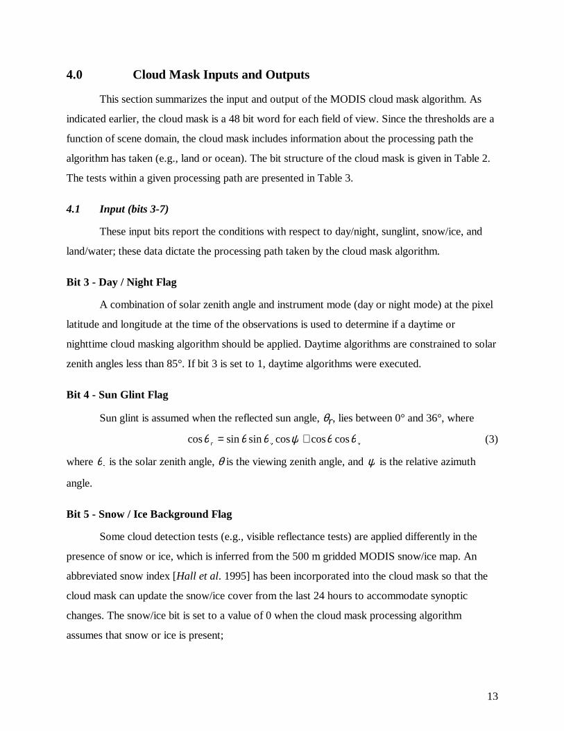
Bit 3 - Day / Night Flag

A combination of solar zenith angle and instrument mode (day or night mode) at the pixel

latitude and longitude at the time of the observations is used to determine if a daytime or

nighttime cloud masking algorithm should be applied. Daytime algorithms are constrained to solar

zenith angles less than 85°. If bit 3 is set to 1, daytime algorithms were executed.

Bit 4 - Sun Glint Flag

Sun glint is assumed when the reflected sun angle, θr, lies between 0° and 36°, where

cos sin sin cos cos cosθ θ θ ψ θ θr = +o o

(3)

where θo

is the solar zenith angle, θ is the viewing zenith angle, and ψ is the relative azimuth

angle.

Bit 5 - Snow / Ice Background Flag

Some cloud detection tests (e.g., visible reflectance tests) are applied differently in the

presence of snow or ice, which is inferred from the 500 m gridded MODIS snow/ice map. An

abbreviated snow index [Hall et al. 1995] has been incorporated into the cloud mask so that the

cloud mask can update the snow/ice cover from the last 24 hours to accommodate synoptic

changes. The snow/ice bit is set to a value of 0 when the cloud mask processing algorithm

assumes that snow or ice is present;

14

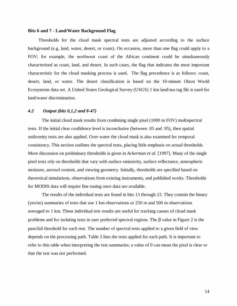
Bits 6 and 7 - Land/Water Background Flag

Thresholds for the cloud mask spectral tests are adjusted according to the surface

background (e.g. land, water, desert, or coast). On occasion, more than one flag could apply to a

FOV; for example, the northwest coast of the African continent could be simultaneously

characterized as coast, land, and desert. In such cases, the flag that indicates the most important

characteristic for the cloud masking process is used. The flag precedence is as follows: coast,

desert, land, or water. The desert classification is based on the 10-minute Olson World

Ecosystems data set. A United States Geological Survey (USGS) 1 km land/sea tag file is used for

land/water discrimination.

4.2 Output (bits 0,1,2 and 8-47)

The initial cloud mask results from combining single pixel (1000 m FOV) multispectral

tests. If the initial clear confidence level is inconclusive (between .05 and .95), then spatial

uniformity tests are also applied. Over water the cloud mask is also examined for temporal

consistency. This section outlines the spectral tests, placing little emphasis on actual thresholds.

More discussion on preliminary thresholds is given in Ackerman et al. [1997]. Many of the single

pixel tests rely on thresholds that vary with surface emissivity, surface reflectance, atmospheric

moisture, aerosol content, and viewing geometry. Initially, thresholds are specified based on

theoretical simulations, observations from existing instruments, and published works. Thresholds

for MODIS data will require fine tuning once data are available.

The results of the individual tests are found in bits 13 through 23. They contain the binary

(yes/no) summaries of tests that use 1 km observations or 250 m and 500 m observations

averaged to 1 km. These individual test results are useful for tracking causes of cloud mask

problems and for isolating tests in user preferred spectral regions. The β value in Figure 2 is the

pass/fail threshold for each test. The number of spectral tests applied to a given field of view

depends on the processing path. Table 3 lists the tests applied for each path. It is important to

refer to this table when interpreting the test summaries; a value of 0 can mean the pixel is clear or

that the test was not performed.

15

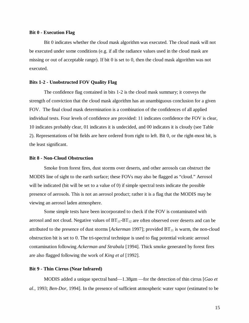
Bit 0 - Execution Flag

Bit 0 indicates whether the cloud mask algorithm was executed. The cloud mask will not

be executed under some conditions (e.g. if all the radiance values used in the cloud mask are

missing or out of acceptable range). If bit 0 is set to 0, then the cloud mask algorithm was not

executed.

Bits 1-2 - Unobstructed FOV Quality Flag

The confidence flag contained in bits 1-2 is the cloud mask summary; it conveys the

strength of conviction that the cloud mask algorithm has an unambiguous conclusion for a given

FOV. The final cloud mask determination is a combination of the confidences of all applied

individual tests. Four levels of confidence are provided: 11 indicates confidence the FOV is clear,

10 indicates probably clear, 01 indicates it is undecided, and 00 indicates it is cloudy (see Table

2). Representations of bit fields are here ordered from right to left. Bit 0, or the right-most bit, is

the least significant.

Bit 8 - Non-Cloud Obstruction

Smoke from forest fires, dust storms over deserts, and other aerosols can obstruct the

MODIS line of sight to the earth surface; these FOVs may also be flagged as “cloud.” Aerosol

will be indicated (bit will be set to a value of 0) if simple spectral tests indicate the possible

presence of aerosols. This is not an aerosol product; rather it is a flag that the MODIS may be

viewing an aerosol laden atmosphere.

Some simple tests have been incorporated to check if the FOV is contaminated with

aerosol and not cloud. Negative values of BT11-BT12 are often observed over deserts and can be

attributed to the presence of dust storms [Ackerman 1997]; provided BT11 is warm, the non-cloud

obstruction bit is set to 0. The tri-spectral technique is used to flag potential volcanic aerosol

contamination following Ackerman and Strabala [1994]. Thick smoke generated by forest fires

are also flagged following the work of King et al [1992].

Bit 9 - Thin Cirrus (Near Infrared)

MODIS added a unique spectral band—1.38µm —for the detection of thin cirrus [Gao et

al., 1993; Ben-Dor, 1994]. In the presence of sufficient atmospheric water vapor (estimated to be

16

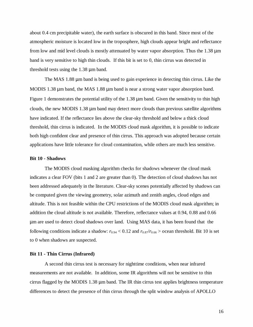
about 0.4 cm precipitable water), the earth surface is obscured in this band. Since most of the

atmospheric moisture is located low in the troposphere, high clouds appear bright and reflectance

from low and mid level clouds is mostly attenuated by water vapor absorption. Thus the 1.38 µm

band is very sensitive to high thin clouds. If this bit is set to 0, thin cirrus was detected in

threshold tests using the 1.38 µm band.

The MAS 1.88 µm band is being used to gain experience in detecting thin cirrus. Like the

MODIS 1.38 µm band, the MAS 1.88 µm band is near a strong water vapor absorption band.

Figure 1 demonstrates the potential utility of the 1.38 µm band. Given the sensitivity to thin high

clouds, the new MODIS 1.38 µm band may detect more clouds than previous satellite algorithms

have indicated. If the reflectance lies above the clear-sky threshold and below a thick cloud

threshold, thin cirrus is indicated. In the MODIS cloud mask algorithm, it is possible to indicate

both high confident clear and presence of thin cirrus. This approach was adopted because certain

applications have little tolerance for cloud contamination, while others are much less sensitive.

Bit 10 - Shadows

The MODIS cloud masking algorithm checks for shadows whenever the cloud mask

indicates a clear FOV (bits 1 and 2 are greater than 0). The detection of cloud shadows has not

been addressed adequately in the literature. Clear-sky scenes potentially affected by shadows can

be computed given the viewing geometry, solar azimuth and zenith angles, cloud edges and

altitude. This is not feasible within the CPU restrictions of the MODIS cloud mask algorithm; in

addition the cloud altitude is not available. Therefore, reflectance values at 0.94, 0.88 and 0.66

µm are used to detect cloud shadows over land. Using MAS data, it has been found that the

following conditions indicate a shadow: r0.94 < 0.12 and r0.87/r0.66 > ocean threshold. Bit 10 is set

to 0 when shadows are suspected.

Bit 11 - Thin Cirrus (Infrared)

A second thin cirrus test is necessary for nighttime conditions, when near infrared

measurements are not available. In addition, some IR algorithms will not be sensitive to thin

cirrus flagged by the MODIS 1.38 µm band. The IR thin cirrus test applies brightness temperature

differences to detect the presence of thin cirrus through the split window analysis of APOLLO

17

and the tri-spectral approach of Strabala et al [1994]. The IR thin cirrus bit 11 is set to 0 when

thin cirrus was detected using infrared bands.

Bit 12 - Adjacent Clouds

If a pixel is clear, adjacent pixels will be searched for low confidence clear flags. If any are

found, this adjacent cloud bit will be set to 0.

Bit 13 - BT Threshold

Several infrared window brightness temperature threshold and temperature difference tests

have been developed; they are most effective at night for cold clouds over water and must be used

with caution in other situations. The primary infrared test over the oceans checks if BT11 is less

than 270 K; if so the pixel fails the clear-sky condition. The α, β, and γ thresholds (see Figure 2)

over ocean are 267 K, 270 K and 273 K.

Bit 14 - CO2 Spectral Band Test for High Clouds

CO2 slicing [Smith et al 1978; Wylie and Menzel 1989] can be used to determine effective

cloud amount and height of high clouds. Due to CPU considerations, simplified tests using the

CO2 bands are used for high cloud detection. Whether a cloud is sensed by a CO2 band depends

upon the atmospheric attenuation in that band and the altitude of the cloud. The spectral band at

13.9 µm provides good sensitivity to the relatively cold regions of the atmosphere. Only clouds

above 500 hPa will have strong contributions to the radiance to space observed at 13.9 µm;

negligible contributions come from the earth’s surface. Thus a threshold test for cloud versus

ambient atmosphere is used to flag high clouds. Initial thresholds are based on HIRS/2

observations, but will have to be modified to the MODIS spectral bands after launch.

Bit 15 - H2O Spectral Band Test for High Clouds

The MODIS spectral band at 6.7 µm provides good sensitivity to the relatively cold

regions of the atmosphere, and will see only clouds above 500 hPa. A threshold test for cloud

versus ambient atmosphere is used to flag cloud contaminated regions. Additionally, methods for

using BT11 and BT6.7 observations to detect upper tropospheric clouds have been developed

[Soden and Bretherton, 1993]. These two bands in combination are especially useful for cloud

18

detection over polar regions during winter. Under clear-sky conditions, strong surface radiative

temperature inversions can develop during winter as a result of longwave energy loss from the

surface through a dry atmosphere. In these conditions, IR bands sensing radiation from low in the

atmosphere will often have a warmer brightness temperature than a window band. Large negative

differences in BT11-BT6.7 exist over the Antarctic Plateau and Greenland during their respective

winters [Ackerman 1996]. This brightness temperature difference is an asset to detecting cloud-

free conditions over elevated surfaces in the polar night [Ackerman 1996]. Clouds inhibit the

formation of the inversion and obscure the inversion from satellite detection if the ice water path

is greater than approximately 20 g m-2. A positive difference of BT11-BT6.7 indicates cloud;

differences more negative than -10C produce high confidence of clear conditions. This test is

applied only during the polar winter.

Bit 16 - R1.38 Test

This test for cirrus cloud uses the MODIS 1.38 µm band [Gao et al., 1993; Ben-Dor,

1994]. It complements the thin cirrus Bit 9. The Bit 16 test uses a larger reflectance threshold

and thus flags thick cirrus not flagged by Bit 9.

Bit 17 - BT3.7 - BT12 Test

The shortwave minus longwave infrared window brightness temperature difference test is

applied during the nighttime. This difference is useful for separating thin cirrus and cloud free

conditions and is relatively insensitive to the amount of water vapor in the atmosphere [Hutchison

and Hardy, 1995]. Bit 17 supplements Bits 9, 11, and 16.

Bit 18 - BT11 - BT12 and BT8.6 - BT11 Test

Over regions where the surface emits like a greybody, spectral tests within various

atmospheric windows can be used to detect the presence of a cloud. Differences between BT11

and BT12 are widely used for cloud screening with AVHRR measurements, often referred to as

the split window technique. Saunders and Kriebel [1988] used BT11-BT12 to detect cirrus clouds

- brightness temperature differences are greater over clouds than clear conditions. Cloud

thresholds are set as a function of satellite zenith angle and BT11. Inoue [1987] also used BT11-

BT12 versus BT11 to separate clear from cloudy conditions. A tri-spectral combination of

19

observations at 8.6, 11 and 12 µm was suggested for detecting clouds and inferring cloud

properties by Ackerman et al. [1990]. Strabala et al. [1994] and Frey et al. [1995] further

explored this technique. The basis of the split window and tri-spectral technique for cloud

detection lies in the differential water vapor absorption that exists between different window

bands (8.6 and 11 µm and 11 and 12 µm).

Brightness temperature difference testing can also be applied over land with careful

consideration of variation in spectral emittance. For example, BT8.6-BT11 has large negative values

over daytime desert and is driven to positive differences in the presence of cirrus.

Bit 19 - BT11 - BT3.9 Test

The MODIS band at 3.9 µm measures radiances in the shortwave infrared window region

near 3.5-4 µm. The difference between BT11 and BT3.9 can be used to detect the presence of

clouds. At night, negative values for BT11-BT3.9 indicate partial cloud or thin cloud within the

MODIS FOV; BT3.9 responds more to the warm fraction of the FOV than BT11 does. Small

differences are observed only when opaque scenes (such as thick cloud or the surface) fill the

FOV.

During the daylight hours, BT11-BT3.9 becomes large negative with reflection of solar

energy at 3.9 µm. This often reveals low level water clouds. BT11-BT3.9 is not useful over deserts

during daytime, as bright desert regions with highly variable emissivities tend to be classified

incorrectly as cloudy. Experience indicates that the thresholds for detecting cloud with BT11-BT3.9

need to be adjusted according to ecosystem type.

Bit 20 - Visible Reflectance Test

This is a single band threshold test that does well for discriminating bright clouds over

dark surfaces (e.g., stratus over ocean) and poorly for clouds over bright surfaces (e.g., snow).

The 0.66 µm (band 1) is used over land and coastal regions. The reflectance test is adjusted for

viewing angle and is also applied in sun glint regions as identified by the sun glint test. The 0.88

µm reflectance test is applied over ocean scenes.

20

Bit 21 - Reflectance Ratio Test

The reflectances in 0.87 and 0.66 µm.are similar over clouds and different over water and

vegetation. Using AVHRR data this ratio, r r. .87 66 , has been found to be between 0.8 and 1.1 in

cloudy regions [Saunders and Kriebel 1988; McClain 1993]. The Global Environment

Monitoring Index (GEMI) attempts to correct for atmospheric effects in deriving a vegetation

index [Pinty and Verstraete 1992; Leprieur et al. 1996]. We have found this approach to be a

better discriminator of cloud. The test,

η η η( . ).

;( ) . .

..

.

. . . .

. .

1 0250125

1

2 15 05

0587

87

66 87 66 87

66 87

− −−−

=− + +

+ +r

r

r r r r

r r

denotes cloudy conditions when η is less than a given threshold. This test does not work well

over desert or coastal scenes, and therefore is not executed in these ecosystems.

Bit 22 - NIR Reflectance Test

Clouds that are low in the atmosphere are often difficult to detect with infrared

techniques. The thermal contrast between clear-sky and low cloud is small and sometimes

undetectable. Reflectance techniques, including the reflectance ratio test can be applied during

daylight hours over certain ecosystems. Use of the MODIS band at 0.936 µm offers help under

daytime viewing conditions. As documented by the work of Gao and Goetz [1991], this band is

strongly affected by low level moisture. When low clouds are present, they obstruct the low level

moisture, and hence increase the reflectance at 0.936 µm.

Bit 23 - BT3.7 - BT3.9 Test

The spectral variation in surface emissivity can present difficulties in applying the

brightness temperature difference tests using BT3.7, BT11, and BT12. Brightness temperature

differences between BT3.7 and BT3.9 reduce this problem for some ecosystems. During the

daylight hours BT3.7 - BT3.9 increases because of the increased solar energy at 3.7 µm.

Bit 24 - Temporal Consistency

Composite clear-sky infrared observations over ocean surfaces will be used to increase

confidence of clear/cloudy scene identifications. Composite maps have been found to be very

21

useful by ISCCP. The MODIS cloud mask will use composite maps, but probably rely on them to

a lesser extent since the advantages of higher spatial resolution and more spectral bands will

change the application and the need.

The lack of reflected solar energy during nighttime processing has the overall effect of

decreasing confidence in the cloud mask output. Some confidence can be restored by using clear-

sky data maps. Cloud-cleared 11 µm brightness temperatures from daytime processing are used as

input to the nighttime cloud masking algorithm. Single-pixel, high confidence (Q > 0.95) clear-sky

values of brightness temperatures, obtained by the MODIS cloud masking algorithm during

daylight hours when solar reflectance is available, will be incorporated into an eight-day

composite equal-area grid at 25 km resolution. The composite data set will be updated after each

day is processed, so that clear-sky observations from day one of the previous eight days will be

eliminated and those from the current day will be added. The eight day cycle was chosen because

seasonal changes in ocean temperature will be adequately represented and because eight days

equals the precession period of high-inclination polar orbiting satellites. Mean, maximum and

minimum values of BT11 will be made available to the nighttime cloud mask algorithm.

Even though the final output of the cloud mask is given by only four confidences of non-

obstructed surface (Q > 0.99, Q > 0.95, Q > 0.66, and Q < 0.66), internally the algorithm has four

additional confidence levels (Q > 0.34, Q > 0.05, Q > 0.01, and Q ≤ 0.01). The algorithm assigns

a confidence value to each single pixel. After an initial assessment, the BT11 of each pixel will be

compared to the daytime composite values from the appropriate grid box. This comparison is

designed to detect inconsistencies between the instantaneous pixel IR measurement and an

expected confidence value (for that measurement) based on the previous eight days of data. If the

observed value is less than the minimum composite value then the pixel confidence is lowered by

two levels. If the observation is greater than or equal to the minimum but less than the mean then

the confidence is downgraded by only one level. In the same way, confidences are raised when

instantaneous brightness temperatures are greater than the mean and/or maximum composite

values. This method allows for lessened confidence in the basic algorithm when applied in the

absence of solar reflection but also recognizes the validity of the IR threshold tests. It also has the

effect of eliminating many mid-range confidences and adding them to either higher or lower

percentage categories.

22

Bit 25 - Infrared Window Radiance Spatial Uniformity

The infrared window spatial uniformity test (applied on 3 by 3 pixel segments) is effective

over water, but is used with caution in other situations. Most ocean regions are well suited for

spatial uniformity tests; such tests may be applied with less confidence in coastal regions or

regions with large temperature gradients (e.g., the Gulf Stream). The MODIS cloud mask

currently uses a spatial variability test over oceans and large lakes. The tests are used to modify

the confidence of a pixel being clear. If the confidence flag of a pixel is between 0.05 and 0.95,

the variability test is implemented. If the difference between the pixel of interest and all of the

surrounding pixel brightness temperatures is less than 0.5°C, the scene is considered uniform and

the confidence is raised one confidence level.

Surface temperature variability, both spatial and temporal, is larger over land than ocean,

making land scene spatial uniformity tests difficult. Therefore, they are not executed over land.

Bits 26 and 31 - Spare Bits

These spare bits are reserved for future developments.

Bits 32 through 47 - 250 Meter Resolution Flags

The 250 m mask will be based on reflectance tests using only the bands at 0.66 and 0.88

µm (see tests for bits 20 and 21). The results are a simple yes/no decision. The 250 m cloud mask

will be collocated within the 1000 m cloud mask in a fixed way; of the 28 250 m pixels that can be

considered located within a 1000 m pixel, the most centered sixteen will be processed for the

cloud mask. The collocation of the 250 m pixels within the 1 km FOV is discussed in Ackerman et

al. [1997]. Since only two bands will be used to generate the 250 m mask, it is expected to be of

lower quality than the 1 km product. Furthermore, this high resolution mask will only be

generated in daytime, sunglint free oceans, and non-desert regions. The cloud mask at 250 m

resolution does not incorporate the results from the 1 km resolution tests.

It is possible to infer cloud fraction in the 1000 m field of view from the 16 visible pixels

within the 1 km footprint. The cloud fraction would be the number of zeros divided by 16. This

would not be advisable in some situations, such as clouds over snow.

23

5.0 Validation

This section presents some of the strengths and weaknesses of the MODIS cloud mask

algorithm. Validating cloud detection is difficult [Ackerman and Cox 1981; Rossow and Garder,

1993b; Baum et al., 1995]. Two important steps in validation are image interpretation and

quantitative analysis. In image interpretation, an analyst conducts a validation through visual

inspection of the spectral, spatial, and temporal features in a set of composite images. Visual

inspection is an important first step in validating any cloud mask algorithm. The analyst uses

knowledge of and experience with cloud and surface spectral properties to identify obvious

problems. However, visual inspection provides poor quantitative evaluation. More quantitative

validation can be attained through direct pixel by pixel comparison with collocated ground or

instrument platform based observations, such as lidar. While this approach provides quantitative

accuracy, it possesses the problem that the two measurement systems often observe different

cloud properties [Baum et al., 1995]. This section provides some validation examples using

image interpretation and quantitative analysis.

In preparation for a MODIS day-1 cloud mask product, observations from the MODIS

Airborne Simulator (MAS) [King et al. 1996], AVHRR, and the HIRS/2 [Frey et al. 1995] are

being used to develop a multispectral cloud mask algorithm. The AVHRR and HIRS/2

instruments fly on the NOAA polar orbiting satellites providing global coverage, while the MAS

flies onboard NASA’s high altitude ER-2 aircraft collecting 50 m resolution data in 50 visible and

infrared spectral bands across a 37 km swath. The basic data sets currently being used to develop

the cloud mask algorithm are listed in Table 4, as well as brief descriptions of the advantages and

disadvantages of each data set. This section provides examples of the MODIS cloud mask

algorithm approach using AVHRR and MAS observations.

5.1 Image interpretation

Figure 3 shows NOAA-14 AVHRR global area coverage (GAC) observations. The left

panel is the 0.6 µm image and the middle panel is the 11 µm image. The scene is over the tropical

Pacific Ocean. The resulting cloud mask output file is represented in the right panel. The legend is

as follows:

Black: Confident of clear (bits 1-2 equal 11),

24

Dark Gray: Probably clear (bits 1-2 equal 10),

Light Gray: Undecided(bits 1-2 equal 01), and

White: Low confidence of clear (bits 1-2 equal 00).

Notice that the confidence in the clear-sky scene tends to drop over the sun glint region (see

visible image), as it is difficult to detect clouds in areas affected by sun glint. The multispectral

advantage of MODIS should improve clear-sky detection capabilities in sun glint regions. Other

AVHRR cloud mask examples can be found at http://cimss.ssec.wisc.edu/modis/cldmsk/ack.

AVHRR global data sets are being used to develop clear-sky composite maps. In this

simple and straightforward implementation of clear-sky composite maps, there are several

common problems that are not explicitly addressed. One problem is changing of air masses, which

occurs regularly in mid-latitudes and often at higher frequency than eight days. Changes in lapse

rate and total column precipitable water amounts can lead to invalid composite values for any

given day. However, since the entire algorithm is tuned as much as possible (via threshold test

confidence intervals) to detection of clear sky, as opposed to cloudy sky, it is anticipated that

errors of this kind will not produce very many false clear-sky identifications. Another possible

source of error is due to limb-darkening. Problems can occur when comparing instantaneous

brightness temperatures from large viewing zenith angles with composites taken primarily from

near-nadir views and vice versa. In the former case, lessened confidences near the limb are

possible but this is a general problem in remote sensing with scanning instruments. Discriminating

clear-sky from clouds is more difficult at limb view angles even for expert image analysts. In the

latter case, the same argument is made as before, that the cloud mask algorithm is (properly)

tuned towards maximum cloud detection so that it is more likely to falsely identify a cloud than

clear sky.

The clear sky composite was tested using AVHRR GAC data collected during July, 1985

in the region encompassing 60° north to 40° south latitude and 40° west to 20° east longitude.

This area was chosen because it contains a large range of ocean temperatures as well as

atmospheric and cloud conditions. The AVHRR cloud detection with five spectral bands is

necessarily limited compared to that of the MODIS with 14 spectral bands. However, because

orbital characteristics, coverage, and spatial resolution are comparable, AVHRR was chosen as

the input for the test.

25

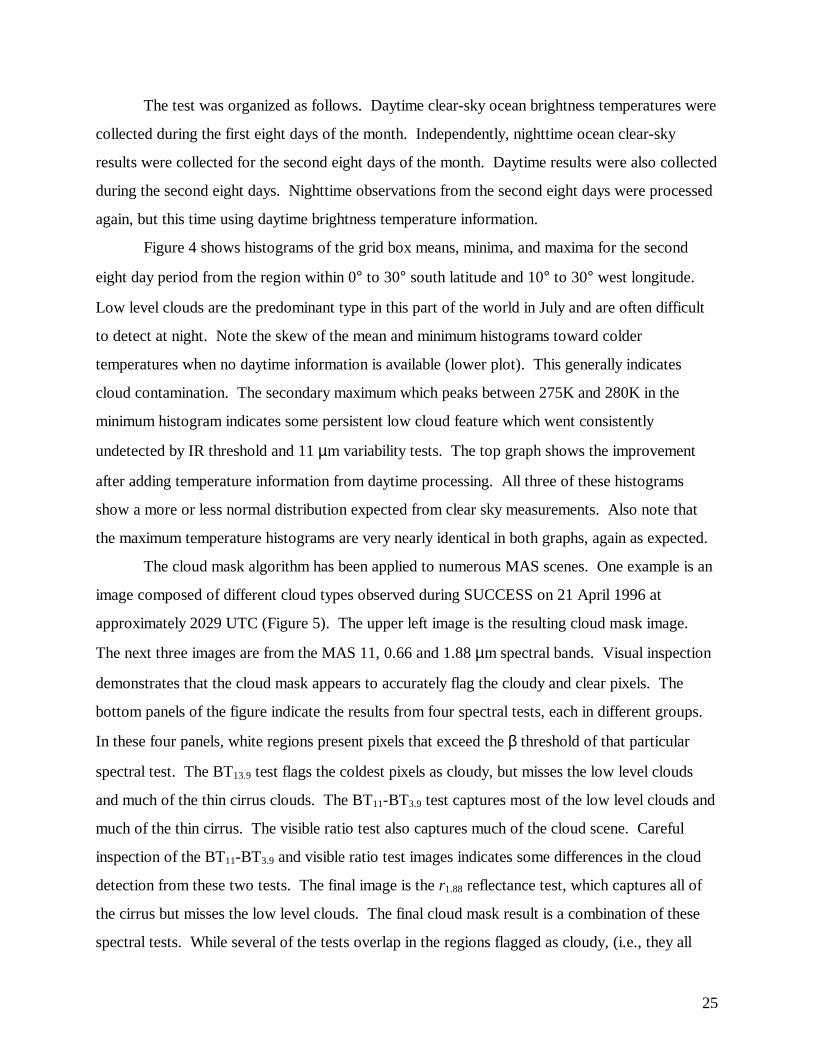
The test was organized as follows. Daytime clear-sky ocean brightness temperatures were

collected during the first eight days of the month. Independently, nighttime ocean clear-sky

results were collected for the second eight days of the month. Daytime results were also collected

during the second eight days. Nighttime observations from the second eight days were processed

again, but this time using daytime brightness temperature information.

Figure 4 shows histograms of the grid box means, minima, and maxima for the second

eight day period from the region within 0° to 30° south latitude and 10° to 30° west longitude.

Low level clouds are the predominant type in this part of the world in July and are often difficult

to detect at night. Note the skew of the mean and minimum histograms toward colder

temperatures when no daytime information is available (lower plot). This generally indicates

cloud contamination. The secondary maximum which peaks between 275K and 280K in the

minimum histogram indicates some persistent low cloud feature which went consistently

undetected by IR threshold and 11 µm variability tests. The top graph shows the improvement

after adding temperature information from daytime processing. All three of these histograms

show a more or less normal distribution expected from clear sky measurements. Also note that

the maximum temperature histograms are very nearly identical in both graphs, again as expected.

The cloud mask algorithm has been applied to numerous MAS scenes. One example is an

image composed of different cloud types observed during SUCCESS on 21 April 1996 at

approximately 2029 UTC (Figure 5). The upper left image is the resulting cloud mask image.

The next three images are from the MAS 11, 0.66 and 1.88 µm spectral bands. Visual inspection

demonstrates that the cloud mask appears to accurately flag the cloudy and clear pixels. The

bottom panels of the figure indicate the results from four spectral tests, each in different groups.

In these four panels, white regions present pixels that exceed the β threshold of that particular

spectral test. The BT13.9 test flags the coldest pixels as cloudy, but misses the low level clouds

and much of the thin cirrus clouds. The BT11-BT3.9 test captures most of the low level clouds and

much of the thin cirrus. The visible ratio test also captures much of the cloud scene. Careful

inspection of the BT11-BT3.9 and visible ratio test images indicates some differences in the cloud

detection from these two tests. The final image is the r1.88 reflectance test, which captures all of

the cirrus but misses the low level clouds. The final cloud mask result is a combination of these

spectral tests. While several of the tests overlap in the regions flagged as cloudy, (i.e., they all

26

detect the thick cirrus cloud) there are regions where certain tests flag clouds which others miss.

This is the advantage of using a variety of spectral tests. The strength of an individual test is a

function of the cloud type, the underlying surface, and the atmospheric temperature and moisture

structure.

Figure 6 is another example of the cloud mask using MAS data as input. The top three

panels are the 0.66, 1.88, and 1.6 µm images made at approximately 1945 UTC on 26 April 1996

over Kansas, US. The 0.66 µm image indicates the presence of a cirrus band extending diagonally

across the image. The 1.88 µm image shows regions of thin cirrus around the thicker cirrus. The

low reflectance regions in the 1.6 µm image are cloud shadows. The final cloud mask result is

displayed in the lower left panel. Most of the scene is flagged as high or low confident clear, very

few pixels are labeled as undecided. Inspection of the cloud mask image with the spectral images

indicates the algorithm is detecting most of the cloud regions. The MODIS cloud mask also

indicates regions of thin cirrus. This is demonstrated in the lower middle panel of Figure 6, where

white regions indicate the presence of thin cirrus. The surface is distinguishable in the 0.66 µm

image where much of the image is flagged as thin cirrus. The thin cirrus flag (optical depth less

than approximately 0.1) is set for regions where land property retrieval algorithms should

incorporate a cloud correction in addition to the atmospheric correction. The lower right-hand

panel of Figure 6 demonstrates the results of the shadow algorithm. The shadow test captures

most of the cloud shadows.

Figure 7 is an example of a scene that has very different meteorological conditions than

the previous ones. The observations were taken over North Dakota on 2 February 1997 at

approximately 1725 UTC. The first panel is the MAS 0.66 µm image and indicates the presence

of a cloud in the upper left hand portion of the image with much of the area covered with snow.

The 1.88 µm image (middle panel) indicates that much of the region is also covered by thin cirrus.

Detection of thin cirrus is lacking in the 0.66 µm image, yet consistent with lidar measurements.

The cloud mask algorithm flagged most of the region as low confidence clear and thin cirrus

contaminated.

27

5.2 Comparison with Collocated Observations

Image visualization is an important component of validating any cloud detection

algorithm. Additional validation includes comparison with active and passive measurements of

clouds. In anticipation of future MODIS cloud mask verification efforts, a prototype methodology

has been developed using the AVHRR cloud mask product. Three complete AVHRR GAC orbits

are processed daily, using the previous day’s level-1b data as input. Daytime coverage includes

the Amazon Basin, Eastern North America, the Saudi Arabian Peninsula, and Central Europe.

Hourly surface observations from ten manned weather stations in North America (ranging in

latitude from 30N to 70N), closest in time to the satellite measurement, are collected and

compared to the cloud mask output. Figure 8 is a 3-D histogram that compares the surface

observation with the closest AVHRR pixel for August and September in 1997. Weather station

cloud reports are plotted on the x-axis and the satellite derived clear sky confidence level on the

y-axis. The z-axis is the frequency of occurrence in each category. Surface observations of

cloudiness are reported as “clear”, “few”, “scattered”, “broken” and “overcast”. Cloud coverage

for these categories is 0/8, 1/8-2/8, 3/8-4/8, 5/8-7/8, and 8/8, respectively. The cloud mask is

generally doing a satisfactory job, particularly for clear skies. This is a result of the conservative

nature of the cloud mask, where only very high confidence pixels are designated as clear. As one

sees more clouds from the ground, the cloud mask confidence for seeing clear sky diminishes, as

expected.

To quantify the MAS cloud mask algorithm performance, comparisons are made with

observations from the Cloud Lidar System (CLS) [Spinhirne and Hart 1990]. During the

SUCCESS, the MAS flew along with the lidar. The CLS algorithm detects a maximum of five

cloud top and cloud bottom altitudes based upon the backscatter signal. Each collocation consists

of the CLS cloud product and approximately 250 to 300 MAS pixels. The percentage of pixels

labeled confident clear, probably clear, uncertain, and low confident clear are determined for each

collocated scene. The CLS observations are divided into three categories:

Clearno cloud was detected by the lidar;

Thin cloudcloud boundary was detected, but a surface return signal was also received;

Thick cloudcloud boundary was detected with no surface return signal.

28

Histograms of the percentage of pixels in a given confidence interval are plotted for each CLS

cloud type category (see Figure 9). Nearly all of the CLS labeled clear scenes are identified as

high confident clear by the MAS cloud mask algorithm. Essentially all of the CLS labeled thick

cloud scenes are labeled as cloudy by the MAS cloud mask. A majority of the thin cloud cases

are labeled as either confident clear or cloudy by the MAS cloud mask algorithm. Differences

between those scenes labeled clear and those classified cloudy are related to the cloud thickness.

A more detailed analysis is required for verification of these thin clouds. Such a study is in

progress. Also encouraging from this comparison is that few of the scenes are labeled as

uncertain. Visualization of the cloud mask indicates that many of these scenes occur near cloud

edges.

6.0 Examples

This section provides examples of how to interpret output from the cloud mask algorithm

for a particular application. They are suggested approaches and not strict rules. Additional

examples are provided in Ackerman et al. [1997].

6.1 Clear scenes only

Certain applications have little tolerance for cloud or shadow contamination. This is an

example of how these applications (e.g., bi-directional reflectance models) might interpret the

cloud mask output.

1. Read bit 0 to determine if a cloud mask was determined; if 0, no further processing of

the pixel is required.

2. If necessary, read bits 3 through 7 to determine scene domain.

3. Read bits 1 and 2; if both bits are not equal to 1, then some tests are suggesting the

presence of the cloud, and the pixel is skipped.

4. Read bit 9 to determine if a thin cirrus cloud is present (bit value of 0). An optically

thin cirrus cloud may set bit 9 but not be classified as a cloudy scene.

5. Read bit 10 to determine if shadow contamination is present; do not process data if

this bit is 0.

6. Daytime algorithms may (depending on application) read bits 32 through 47 to assess

potential subpixel contamination or scene variability.

29

6.2 Clear scenes with thin cloud correction algorithms

Some algorithms may be insensitive to the presence of thin cloud or may apply appropriate

correction algorithms. This is a suggested application; after launch minor modifications may be

implemented depending on the performance of the cloud masking algorithm. An example is

presented that might be appropriate for Normalized Difference Vegetation Index (NDVI).

1. Read bit 0 to determine if a cloud mask was determined; if 0, no further processing of

the pixel is required.

2. Read bits 3 through 7 to determine if scene domain is appropriate (e.g., land and

daytime).

3. Read the confidence flag bits 1 and 2. If cloudy (value of 00), do not process this

pixel. A value of 01 for bits 1 and 2 (uncertain) often occurs around cloud edges and

retrieving NDVI may not be appropriate with this confidence level. If both bits are

equal to 1, then most tests are suggesting clear scenes; proceed with steps 4-7. If

confidence bits are 10, then detailed checking of bits 13 through 25 may be required to

determine if the NDVI retrieval should proceed.

4. Read bit 9 to determine if a thin cirrus cloud is present (bit value of 0). An optically

thin cirrus cloud may set bit 9 but not be classified as a cloudy scene. Some of the

MODIS solar channels are not as sensitive to thin cirrus as the 1.38 µm band (see

Figure 1 for a corresponding example using the MAS 1.88 µm channel). If thin cirrus

is detected, apply appropriate correction algorithms.

5. Check that reflectance tests (bits 20 and 21) did not detect cloud. Note that a value of

0 indicates that either a cloud is present or the test was not run. This test is not run if

over snow or solar zenith angles greater than 85°.

6. Read bit 10 to determine if shadow contamination is present. Shadows might bias the

NDVI product.

7. Read bits 32 through 47 to assess cloud contamination. This would not be

recommended if snow is indicated.

30

6.3 Cloud retrieval algorithms

Use of the cloud mask for cloud scene processing may require a more in-depth analysis

than clear-sky applications, as the mask is clear-sky conservative. An approach to interpreting the

cloud mask for cloud property retrievals during the day over ocean scenes in non-sunglint regions

is outlined.

1. Read bit 0 to determine if a cloud mask was determined; if 0, no further processing of

the pixel is required.

2. Read bit 3; if 0, no further processing of the pixel is required (night).

3. Read bits 6 and 7; if 00 then proceed (water).

4. Read bit 4; if 0 then it is a sunglint region. The user may want to place less confidence

on a product retrieval.

5. Read the confidence flag bits 1 and 2.

• If confident clear (value of 11), read bit 9 to determine if a thin cirrus cloud is

present (bit value of 0). An optically thin cirrus cloud may set bit 9 but not be

classified as a cloudy scene. If thin cirrus is detected, apply appropriate

algorithms or place less confidence on the product retrieval. If bit 9 is 1, then

no further processing is required.

• If both bits are equal to 00, then the scene is cloudy. Check bit 8 for possible

heavy aerosol loading. If bit 8 is 0, then the pixel may be aerosol contaminated.

In this case no further processing is necessary or place less confidence on the

product retrieval.

• If confidence is 10 or 01, then detailed checking of bits 13 through 25 may be

required to determine if the retrieval algorithm should be executed. For

example, if confidence bits are 10 and pixel is in a sun glint region, additional

testing is advised.

6. Check how many tests detected cloud. The greater the number of tests that detected

cloud, the more confidence one has in the cloud property product. Note that a value of

0 indicates that either a cloud is present or the test was not run.

7. Check spatial variability test results.

31

8. Read bits 32 through 47 to assess subpixel cloud contamination. This would not be

recommended for regions with sun glint.

7.0 Summary

The MODIS cloud mask is more than a simple yes/no decision. The cloud mask includes 4

levels of confidence whether a pixel is clear (bits 1 and 2) as well as the results from different

spectral tests. An individual confidence flag is assigned to each single pixel test and is a function

of how close the observation is to the threshold. The individual confidence flags are combined to

produce the final cloud mask flag for the output file.

The MODIS cloud mask algorithm is divided into several conceptual domains according

to surface type and solar illumination. Each domain defines a processing path through the

algorithm, which in turn defines the spectral tests performed and associated thresholds. Different

cloud conditions are detected by different tests. Spectral tests which find similar cloud conditions

are grouped together. The groups are arranged so that independence between them is maximized,

but few, if any, spectral tests are completely independent of all the others.

Example cloud masks from AVHRR and MAS data reveal that most observations have

either high confidences (Q > 0.95) or very low confidences (Q < 0.05) of unobstructed views of

the surface. However, there are always those difficult scenes which result in intermediate

confidence of the clear sky. These tend to be found at cloud boundaries, or where low clouds are

found over water surfaces at night, or over certain land surfaces such as desert or other sparsely-

vegetated regions. In these cases (Q > 0.05 and Q < 0.95), spatial and/or temporal continuity tests

are conducted.

Initial validation of the cloud mask algorithm has been accomplished with visual inspection

of imagery, comparison with surface cloud observations, and comparison with lidar retrievals.

While the results show good agreement, it is anticipated that considerable adjustment to the

algorithm will be necessary in the first six months after MODIS launch. Routine and reliable

production of the MODIS cloud mask is anticipated in late 1998.

Acknowledgments. The authors would like to graciously thank Bryan Baum, Crystal Shaaf,

George Riggs, Michael King, Si-Chee Tsay, North Larsen, Jason Li, Chris Sisko and Yoram

32

Kaufman for their help in the development and testing of the MODIS cloud mask. We would also

like to thank Jim Spinhirne and his research group for providing lidar data used in cloud mask

validation. This research was funded under NASA grant NAS5-31367. NASA grants NAG5-3193

and NAGW-3318 also contributed to MAS data collection during SUCCESS.

8.0 References

Ackerman, S. A., and S. K. Cox, 1981: Comparison of satellite and all-sky camera estimates of cloud

cover during GATE. J. Appl. Meteor., 20, 581-587.

Ackerman, S. A., 1997: Remote sensing aerosols from satellite infrared observations. J. Geophys.

Res., 102, 17069-17079.

Ackerman, S. A., K. I. Strabala, W. P. Menzel, R. A. Frey, C. C. Moeller, L. E. Gumley, B. A.

Baum, C. Schaaf, G. Riggs, 1997: Discriminating clear-sky from cloud with MODIS

algorithm theoretical basis document (MOD35). EOS ATBD web site, 125 pp.

Ackerman, S. A., 1996: Global satellite observations of negative brightness temperature

difference between 11 and 6.7 µm. J. Atmos. Sci. 53, 2803-2812.

Ackerman, S. A., K. I. Strabala, 1994: Satellite remote sensing of H2SO4 aerosol using the 8 - 12

µm window region: Application to Mount Pinatubo. J. Geo. Res. 99, 18,639-18,649.

Ackerman, S. A., W. L. Smith and H. E. Revercomb, 1990: The 27-28 October 1986 FIRE IFO

cirrus case study: Spectral properties of cirrus clouds in the 8-12 µm window. Mon. Wea.

Rev., 118, 2377-2388.

Baum, B. A., T. Uttal, M. Poellot, T. P. Ackerman, J. M. Alvarez, J. Intrieri, D. O’C. Starr, J.

Titlow, V. Tovinkere, and E. Clothiaux, 1995: Satellite remote sensing of multiple cloud

layers. J. Atmos. Sci., 52, 4210-4230.

33

Ben-Dor, E., 1994: A precaution regarding cirrus cloud detection from airborne imaging

spectrometer data using the 1.38 µm water vapor band. Remote Sens. Environ., 50, 346-

350.

Frey, R. A., S. A. Ackerman, and B. J. Soden, 1995: Climate parameters from satellite spectral

measurements. Part I: Collocated AVHRR and HIRS/2 observations of the spectral

greenhouse parameter. Jour. Clim. 9, 327-344.

Gao, B.-C., A. F. H. Goetz, and W. J. Wiscombe, 1993: Cirrus cloud detection from airborne

imaging spectrometer data using the 1.38 µm water vapor band. Geophys. Res. Lett., 20,

301-304.

Gao, B.-C., and A. F. H. Goetz, 1991: Cloud area determination from AVIRIS data using water

vapor channels near 1 µm. J. Geophys. Res., 96, 2857-2864.

Gesell, G., 1989: An algorithm for snow and ice detection using AVHRR data: An extension to

the APOLLO software package. Int. J. Remote Sensing, 10, 897-905.

Hall, D.K., Riggs, G.A. and Salomonson, V.V. 1995: Development of methods for mapping

global snow cover using Moderate Resolution Imaging Spectroradiometer data, Remote

Sens. Env., 54,127-140.

Hutchison, K. D., and K. R. Hardy, 1995: Threshold functions for automated cloud analyses of

global meteorological satellite imagery. Int. J. Remote Sens., 16, 3665-3680.

Inoue, T., 1987: A cloud type classification with NOAA 7 split window measurements. J.

Geophys. Res., 92, 3991-4000.

King, M. D., Y. J. Kaufman, W. P. Menzel and D. Tanré, 1992: Remote sensing of cloud,

aerosol, and water vapor properties from the Moderate Resolution Imaging Spectrometer

(MODIS). IEEE Trans. Geosci. Remote Sens., 30, 2–27.

King, M. D., W. P. Menzel, P. S. Grant, J. S. Myers, G. T. Arnold, S. E. Platnick, L. E. Gumley,

S. C. Tsay, C. C. Moeller, M. Fitzgerald, K. S. Brown and F. G. Osterwisch, 1996:

Airborne scanning spectrometer for remote sensing of cloud, aerosol, water vapor and

surface properties. J. Atmos. Oceanic Technol., 13, 777-794.

Kriebel, K. T., and R. W. Saunders, 1988: An improved method for detecting clear sky and

cloudy radiances from AVHRR data. Int. J. Remote Sens., 9, 123-150.

34

Leprieur, C., Y. H. Kerr, and J. M. Pichon, 1996: Critical assessment of vegetation indices from

AVHRR in a semi-arid environment. Int. J. Remote Sensing, 17, 2549-2563.

McClain, E. P., 1993: Evaluation of CLAVR Phase-I algorithm performance. Final Report, U. S.

Department of Commerce/NOAA/NESDIS, Report 40-AANE-201-424.

Menzel, W. P., D. P. Wylie, and K. I. Strabala, 1993. Trends in global cirrus inferred from four

years of HIRS data. Technical Proceedings of the Seventh International TOVS Study

Conference, 10-16 February, Igls, Austria

Pinty, B., and Verstraete, M. M., 1992: GEMI: A non-linear index to monitor global vegetation

from satellites. Vegetation, 101, 15-20.

Rizzi, C. Serio, G. Kelly, V. Tramutoli, A. McNally and V. Cuomo, 1994. Cloud clearing of

infrared sounder radiances. J. Appl. Meteor., 33, 179-194.

Rossow, W. B., 1989: Measuring cloud properties from space. A review. J. Climate, 2, 201-213.

Rossow, W. B. and L. C. Garder, 1993a. Cloud detection using satellite measurements of

infrared and visible radiances for ISCCP. J. Climate, 6, 2341-2369.

Rossow, W. B. and L. C. Garder, 1993b: Validation of ISCCP cloud detections. J. Climate, 6,

2370-2393.

Rossow, W. B., A. W. Walker, and L. C. Garder, 1993: Comparison of ISCCP and other cloud

amounts. J. Climate, 6, 2394-2418.

Saunders, R. W. and K. T. Kriebel, 1988. An improved method for detecting clear sky and

cloudy radiances from AVHRR data. Int. J. Remote Sens., 9, 123-150.

Seze, G., and W. B. Rossow, 1991: Time-cumulated visible and infrared radiance histograms used

as descriptors of surface and cloud variations. Int. J. Remote Sens., 12, 877-920.

Smith, W. L, 1968. An improved method for calculating tropospheric temperature and moisture

profiles from satellite radiometer measurements. Mon. Wea. Rev., 96, 387.

Smith, W. L. and C. M. R. Platt, 1978: Comparison of satellite-deduced cloud heights with

indications from radiosonde and ground-based laser measurements. J. Appl. Meteor., 17,

1796-1802.

Smith, W. L., H. M. Woolf, S. J. Nieman and T. H. Achtor, 1993. ITPP-5 - The use of AVHRR

and TIGR in TOVS Data Processing. Technical Proceedings of the Seventh International

TOVS Study Conference, 10-16 February, Igls, Austria, 443-453.

35

Spinhirne, J. D. and W. D. Hart, 1990. Cirrus structure and radiative properties from airborne

lidar and spectral radiometer observations. Mon. Wea. Rev., 2329.

Soden, B. J. and F. P. Bretherton, 1993: Upper tropospheric relative humidity from the GOES 6.7

µm channel: Method and climatology for July 1987, J. Geo. Res., 98, 16669-16688.

Stowe, L. L., E. P. McClain, R. Carey, P. Pellegrino, G. Gutman, P. Davis, C. Long, and S. Hart,

1991. Global distribution of cloud cover derived from NOAA/AVHRR operational

satellite data. Adv. Space Res., 11, 51-54.

Stowe, L. L., S. K. Vemury, and A. V. Rao, 1994: AVHRR clear sky radiation data sets at

NOAA/NESDIS. Adv. Space Res., 14, 113-116.

Strabala, K. I., S. A. Ackerman, and W. P. Menzel, 1994: Cloud properties inferred from 8-12

µm data. J. Appl. Meteor., 33, 212-229.

Wylie, D. P., and W. P. Menzel, 1989: Two years of cloud cover statistics using VAS. J. Climate

Appl. Meteor., 2, 380-392.

Wylie, D. P., W. P. Menzel, H. M. Woolf, and K. I. Strabala, 1994: Four years of global cirrus

cloud statistics using HIRS. J. Climate, 7, 1972-1986.

36

Figure Captions

Figure 1. Three spectral images (0.66, 1.88 and 11 µm) taken from the MAS during the

SUCCESS experiment (20 April 1996). In the 11 µm image, dark is cold; in the vis/NIR

images, white is high reflectance.

Figure 2. A graphical depiction of three thresholds used in cloud screening.

Figure 3. An example of the cloud mask derived from AVHRR data for a scene over the Pacific

Ocean (right hand panel), together with images from two of the AVHRR bands used in

generating the mask. The legend is as follows: black is high confidence of clear (bits 1-2

equal 11), dark gray is probably clear (bits 1-2 equal 10), light gray is uncertain (bits 1-2

equal 01), and white is cloudy (bits 1-2 equal 00).

Figure 4. Distribution of BT11 in clear-sky conditions with daytime observations (top) and

without (bottom).

Figure 5. Cloud mask algorithm applied to MAS data on 21 April 1996. Images along the top are

cloud mask result, BT11 , r0.66 and r0.188. Results from representative tests in applied

groups are shown in the bottom panels (see text for details).

Figure 6. Example of cloud mask algorithms applied to MAS data on 26 April 1996. The upper

panels are MAS images at 0.66, 1.88, and 1.6 µm. The lower images show the final mask,

thin cirrus mask, and the shadow mask.

Figure 7. Example of the cloud mask algorithm applied to a winter scene on 2 February 1997.

Figure 8. Comparison of surface cloud reports and AVHRR cloud mask results. Note the good

agreement in clear as well as broken and overcast skies.

Figure 9. Comparisons between the cloud detection results using MAS and cloud lidar system for

five days of the SUCCESS experiment. Cloud mask confidence is compared with three

lidar categories: no cloud (top panel), thin cloud (middle panel), and thick cloud (bottom

panel).

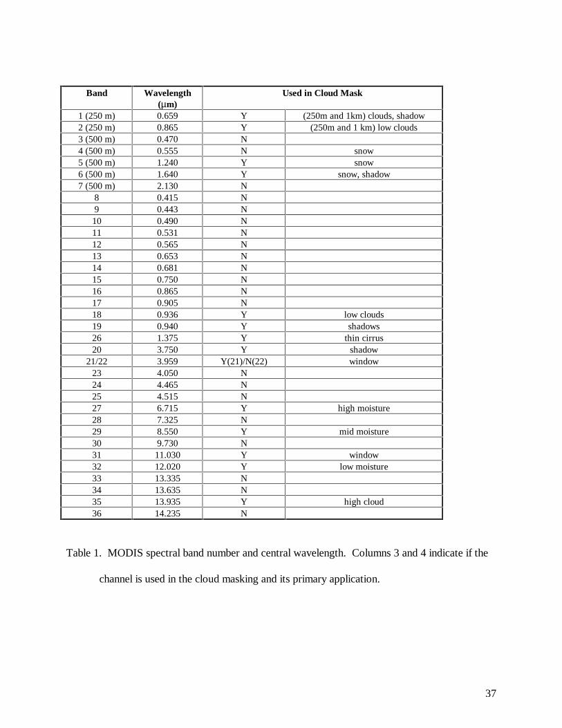
37

Band Wavelength(µm)

Used in Cloud Mask

1 (250 m) 0.659 Y (250m and 1km) clouds, shadow2 (250 m) 0.865 Y (250m and 1 km) low clouds3 (500 m) 0.470 N4 (500 m) 0.555 N snow5 (500 m) 1.240 Y snow6 (500 m) 1.640 Y snow, shadow7 (500 m) 2.130 N

8 0.415 N9 0.443 N10 0.490 N11 0.531 N12 0.565 N13 0.653 N14 0.681 N15 0.750 N16 0.865 N17 0.905 N18 0.936 Y low clouds19 0.940 Y shadows26 1.375 Y thin cirrus20 3.750 Y shadow

21/22 3.959 Y(21)/N(22) window23 4.050 N24 4.465 N25 4.515 N27 6.715 Y high moisture28 7.325 N29 8.550 Y mid moisture30 9.730 N31 11.030 Y window32 12.020 Y low moisture33 13.335 N34 13.635 N35 13.935 Y high cloud36 14.235 N

Table 1. MODIS spectral band number and central wavelength. Columns 3 and 4 indicate if the

channel is used in the cloud masking and its primary application.

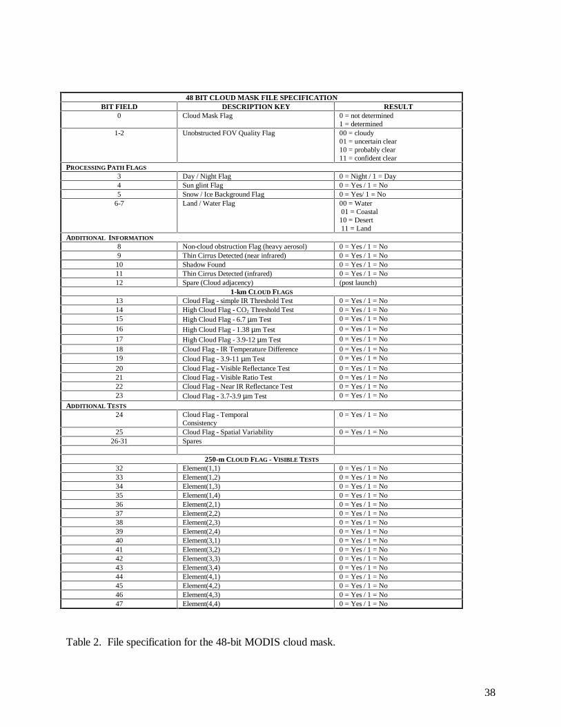
38

48 BIT CLOUD MASK FILE SPECIFICATIONBIT FIELD DESCRIPTION KEY RESULT

0 Cloud Mask Flag 0 = not determined1 = determined

1-2 Unobstructed FOV Quality Flag 00 = cloudy01 = uncertain clear10 = probably clear11 = confident clear

PROCESSING PATH FLAGS

3 Day / Night Flag 0 = Night / 1 = Day4 Sun glint Flag 0 = Yes / 1 = No5 Snow / Ice Background Flag 0 = Yes/ 1 = No

6-7 Land / Water Flag 00 = Water 01 = Coastal10 = Desert 11 = Land

ADDITIONAL INFORMATION

8 Non-cloud obstruction Flag (heavy aerosol) 0 = Yes / 1 = No9 Thin Cirrus Detected (near infrared) 0 = Yes / 1 = No10 Shadow Found 0 = Yes / 1 = No11 Thin Cirrus Detected (infrared) 0 = Yes / 1 = No12 Spare (Cloud adjacency) (post launch)

1-km CLOUD FLAGS

13 Cloud Flag - simple IR Threshold Test 0 = Yes / 1 = No14 High Cloud Flag - CO2 Threshold Test 0 = Yes / 1 = No15 High Cloud Flag - 6.7 µm Test 0 = Yes / 1 = No16 High Cloud Flag - 1.38 µm Test 0 = Yes / 1 = No17 High Cloud Flag - 3.9-12 µm Test 0 = Yes / 1 = No18 Cloud Flag - IR Temperature Difference 0 = Yes / 1 = No19 Cloud Flag - 3.9-11 µm Test 0 = Yes / 1 = No20 Cloud Flag - Visible Reflectance Test 0 = Yes / 1 = No21 Cloud Flag - Visible Ratio Test 0 = Yes / 1 = No22 Cloud Flag - Near IR Reflectance Test 0 = Yes / 1 = No23 Cloud Flag - 3.7-3.9 µm Test 0 = Yes / 1 = No

ADDITIONAL TESTS

24 Cloud Flag - TemporalConsistency

0 = Yes / 1 = No

25 Cloud Flag - Spatial Variability 0 = Yes / 1 = No26-31 Spares

250-m CLOUD FLAG - VISIBLE TESTS

32 Element(1,1) 0 = Yes / 1 = No33 Element(1,2) 0 = Yes / 1 = No34 Element(1,3) 0 = Yes / 1 = No35 Element(1,4) 0 = Yes / 1 = No36 Element(2,1) 0 = Yes / 1 = No37 Element(2,2) 0 = Yes / 1 = No38 Element(2,3) 0 = Yes / 1 = No39 Element(2,4) 0 = Yes / 1 = No40 Element(3,1) 0 = Yes / 1 = No41 Element(3,2) 0 = Yes / 1 = No42 Element(3,3) 0 = Yes / 1 = No43 Element(3,4) 0 = Yes / 1 = No44 Element(4,1) 0 = Yes / 1 = No45 Element(4,2) 0 = Yes / 1 = No46 Element(4,3) 0 = Yes / 1 = No47 Element(4,4) 0 = Yes / 1 = No

Table 2. File specification for the 48-bit MODIS cloud mask.

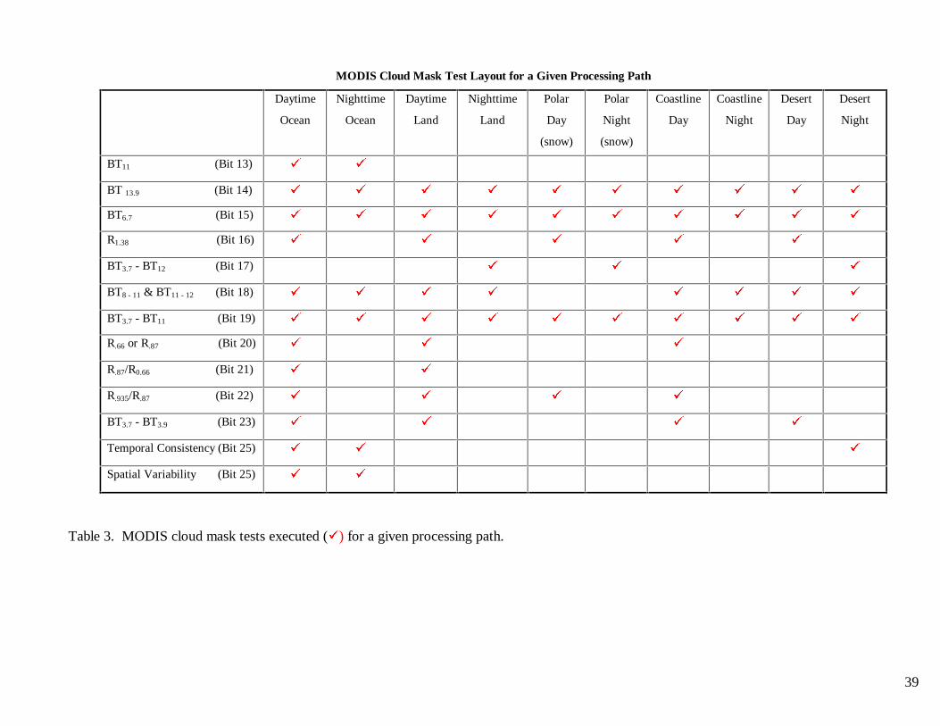
39

MODIS Cloud Mask Test Layout for a Given Processing Path

Daytime

Ocean

Nighttime

Ocean

Daytime

Land

Nighttime

Land

Polar

Day

(snow)

Polar

Night

(snow)

Coastline

Day

Coastline

Night

Desert

Day

Desert

Night

BT11 (Bit 13) ä ä

BT 13.9 (Bit 14) ä ä ä ä ä ä ä ä ä ä

BT6.7 (Bit 15) ä ä ä ä ä ä ä ä ä ä

R1.38 (Bit 16) ä ä ä ä ä

BT3.7 - BT12 (Bit 17) ä ä ä

BT8 - 11 & BT11 - 12 (Bit 18) ä ä ä ä ä ä ä ä

BT3.7 - BT11 (Bit 19) ä ä ä ä ä ä ä ä ä ä

R.66 or R.87 (Bit 20) ä ä ä

R.87/R0.66 (Bit 21) ä ä

R.935/R.87 (Bit 22) ä ä ä ä

BT3.7 - BT3.9 (Bit 23) ä ä ä ä

Temporal Consistency (Bit 25) ä ä ä

Spatial Variability (Bit 25) ä ä

Table 3. MODIS cloud mask tests executed (ä) for a given processing path.

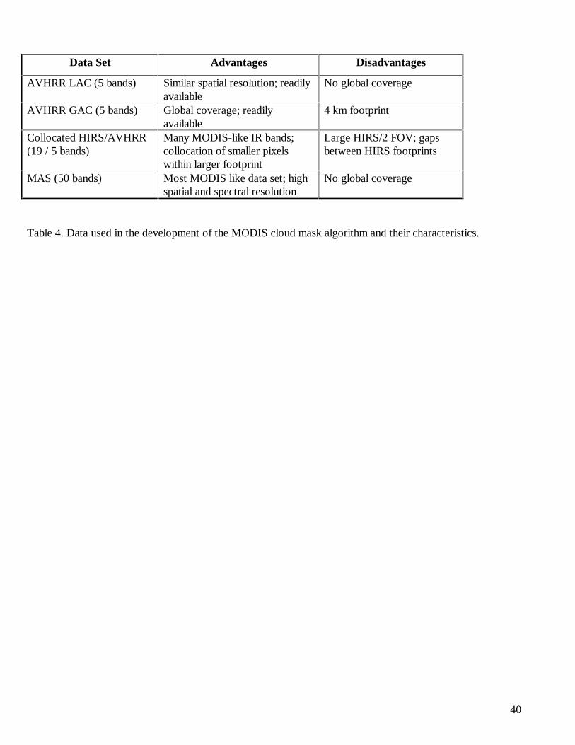
40

Data Set Advantages Disadvantages

AVHRR LAC (5 bands) Similar spatial resolution; readilyavailable

No global coverage

AVHRR GAC (5 bands) Global coverage; readilyavailable

4 km footprint

Collocated HIRS/AVHRR(19 / 5 bands)

Many MODIS-like IR bands;collocation of smaller pixelswithin larger footprint

Large HIRS/2 FOV; gapsbetween HIRS footprints

MAS (50 bands) Most MODIS like data set; highspatial and spectral resolution

No global coverage

Table 4. Data used in the development of the MODIS cloud mask algorithm and their characteristics.

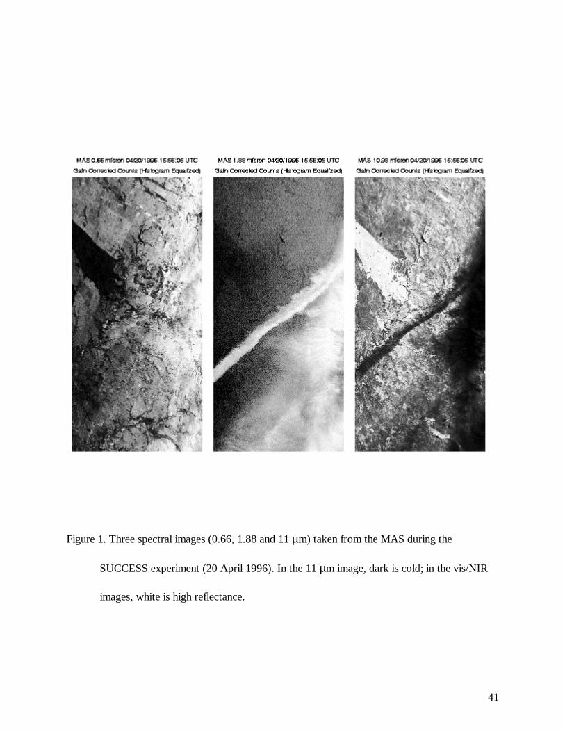
41

Figure 1. Three spectral images (0.66, 1.88 and 11 µm) taken from the MAS during the

SUCCESS experiment (20 April 1996). In the 11 µm image, dark is cold; in the vis/NIR

images, white is high reflectance.

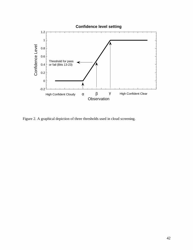
42

Figure 2. A graphical depiction of three thresholds used in cloud screening.

Confidence level setting

Observation

Con

fiden

ce L

evel

-0.2

0

0.2

0.4

0.6

0.8

1

1.2

High Confident Cloudy High Confident Clearα γβ

Threshold for pass or fail (Bits 13-23)

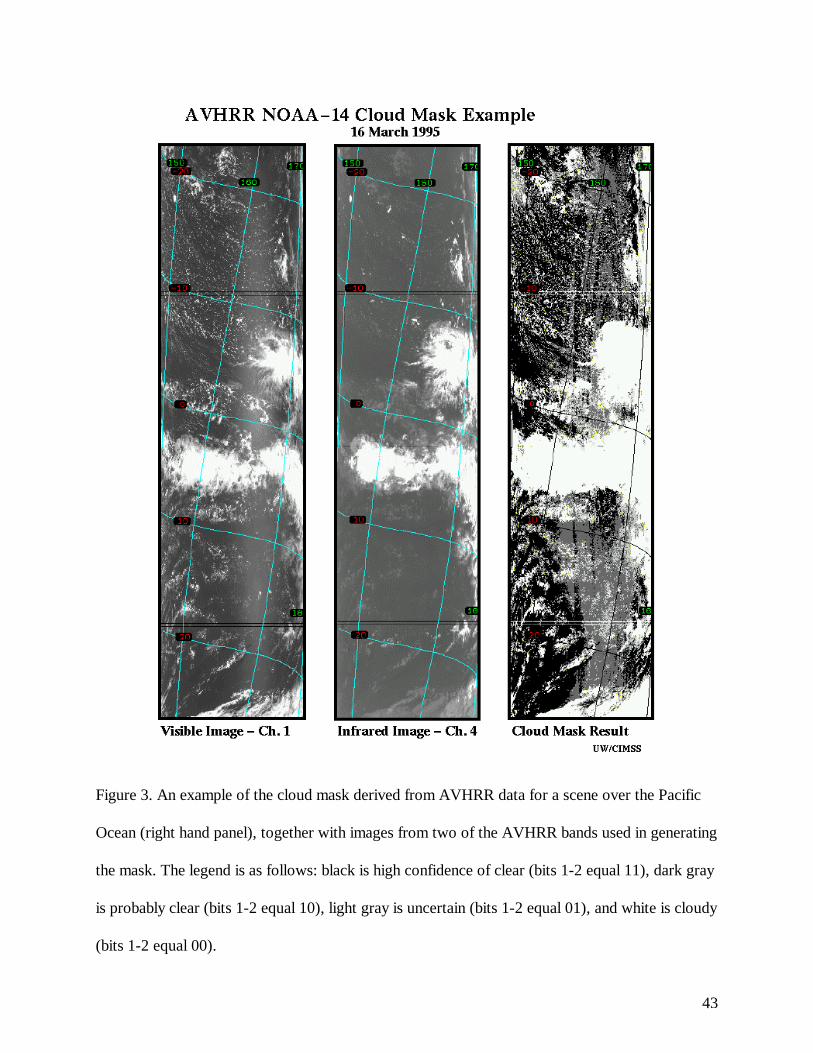
43

Figure 3. An example of the cloud mask derived from AVHRR data for a scene over the Pacific

Ocean (right hand panel), together with images from two of the AVHRR bands used in generating

the mask. The legend is as follows: black is high confidence of clear (bits 1-2 equal 11), dark gray

is probably clear (bits 1-2 equal 10), light gray is uncertain (bits 1-2 equal 01), and white is cloudy

(bits 1-2 equal 00).

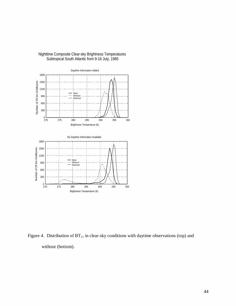
44

Nighttime Composite Clear-sky Brightness TemperaturesSubtropical South Atlantic from 9-16 July, 1985

Daytime Information Added

Brightness Temperature (K)

Num

ber

of 2

5 km

Grid

boxe

s

0

300

600

900

1200

1500

1800

270 275 280 285 290 295 300

MeanMinimumMaximum

No Daytime Information Available

Brightness Temperature (K)

Num

ber

of 2

5 km

Grid

boxe

s

0

300

600

900

1200

1500

1800

270 275 280 285 290 295 300

MeanMinimumMaximum

Figure 4. Distribution of BT11 in clear-sky conditions with daytime observations (top) and

without (bottom).

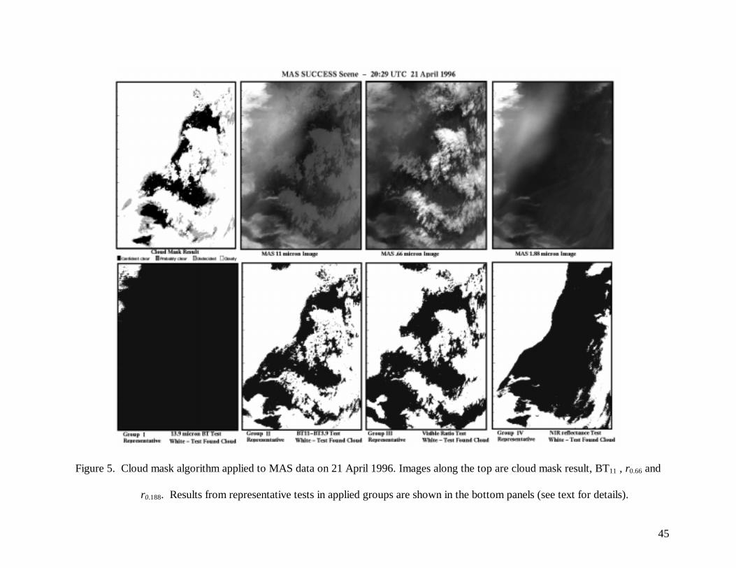
45

Figure 5. Cloud mask algorithm applied to MAS data on 21 April 1996. Images along the top are cloud mask result, BT11 , r0.66 and

r0.188. Results from representative tests in applied groups are shown in the bottom panels (see text for details).

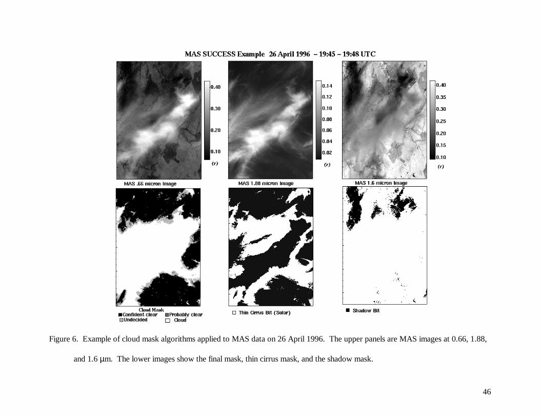
46

Figure 6. Example of cloud mask algorithms applied to MAS data on 26 April 1996. The upper panels are MAS images at 0.66, 1.88,

and 1.6 µm. The lower images show the final mask, thin cirrus mask, and the shadow mask.

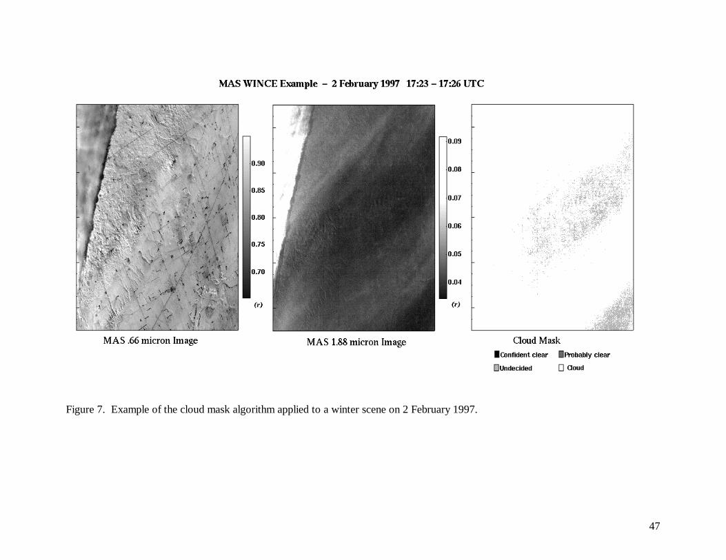
47

Figure 7. Example of the cloud mask algorithm applied to a winter scene on 2 February 1997.

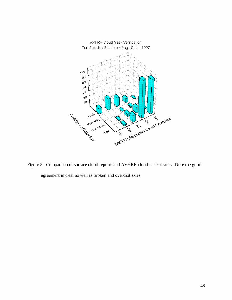
48

Figure 8. Comparison of surface cloud reports and AVHRR cloud mask results. Note the good

agreement in clear as well as broken and overcast skies.

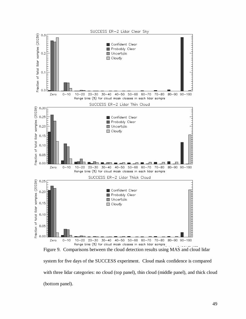
49

Figure 9. Comparisons between the cloud detection results using MAS and cloud lidar

system for five days of the SUCCESS experiment. Cloud mask confidence is compared

with three lidar categories: no cloud (top panel), thin cloud (middle panel), and thick cloud

(bottom panel).