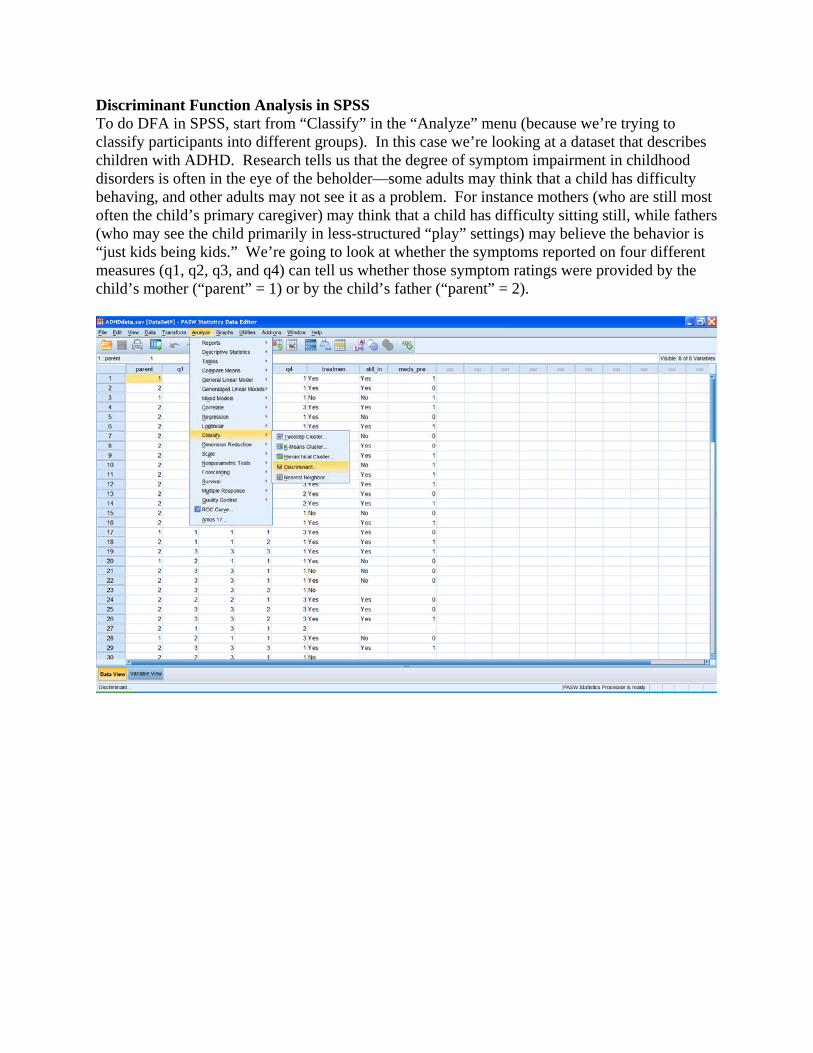
Discriminant Function Analysis in SPSS To do DFA in SPSS, start from “Classify” in the “Analyze” menu (because we’re trying to classify participants into different groups). In this case we’re looking at a dataset that describes children with ADHD. Research tells us that the degree of symptom impairment in childhood disorders is often in the eye of the beholder—some adults may think that a child has difficulty behaving, and other adults may not see it as a problem. For instance mothers (who are still most often the child’s primary caregiver) may think that a child has difficulty sitting still, while fathers (who may see the child primarily in less-structured “play” settings) may believe the behavior is “just kids being kids.” We’re going to look at whether the symptoms reported on four different measures (q1, q2, q3, and q4) can tell us whether those symptom ratings were provided by the child’s mother (“parent” = 1) or by the child’s father (“parent” = 2).

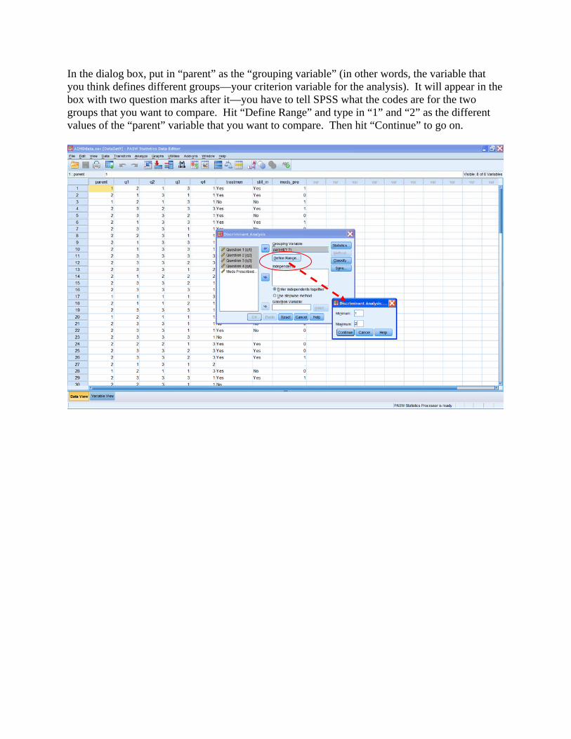
In the dialog box, put in “parent” as the “grouping variable” (in other words, the variable that you think defines different groups—your criterion variable for the analysis). It will appear in the box with two question marks after it—you have to tell SPSS what the codes are for the two groups that you want to compare. Hit “Define Range” and type in “1” and “2” as the different values of the “parent” variable that you want to compare. Then hit “Continue” to go on.

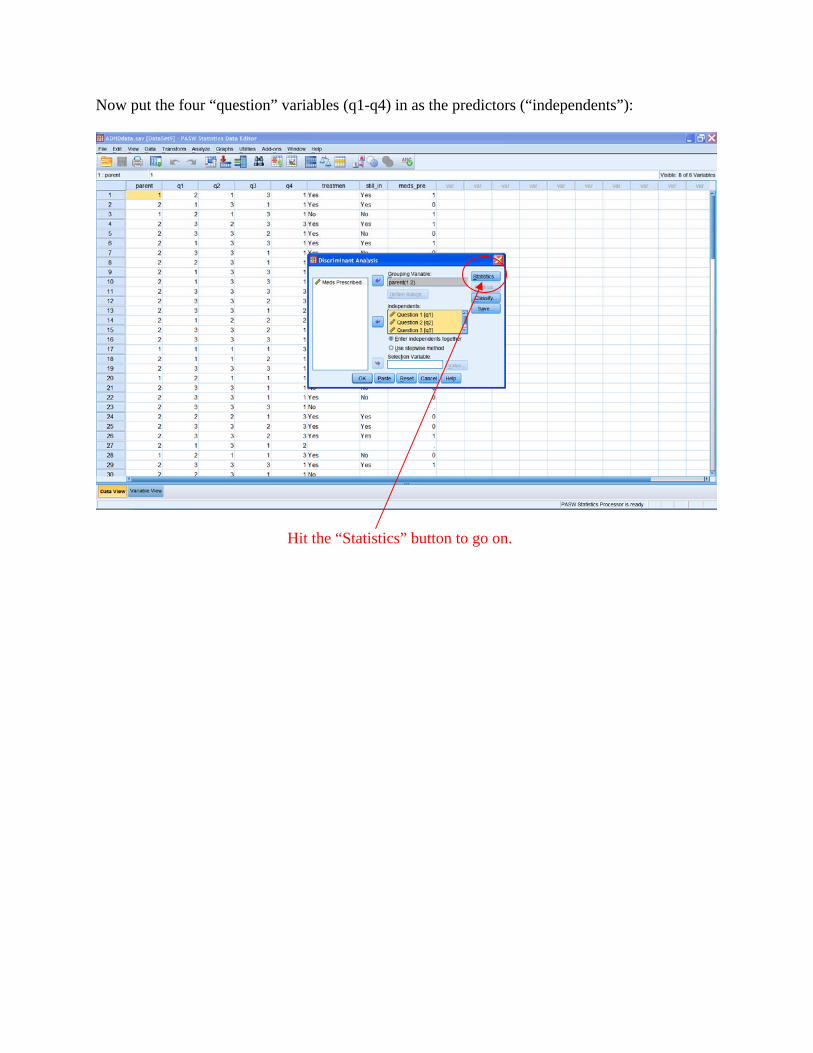
Now put the four “question” variables (q1-q4) in as the predictors (“independents”):

Hit the “Statistics” button to go on.

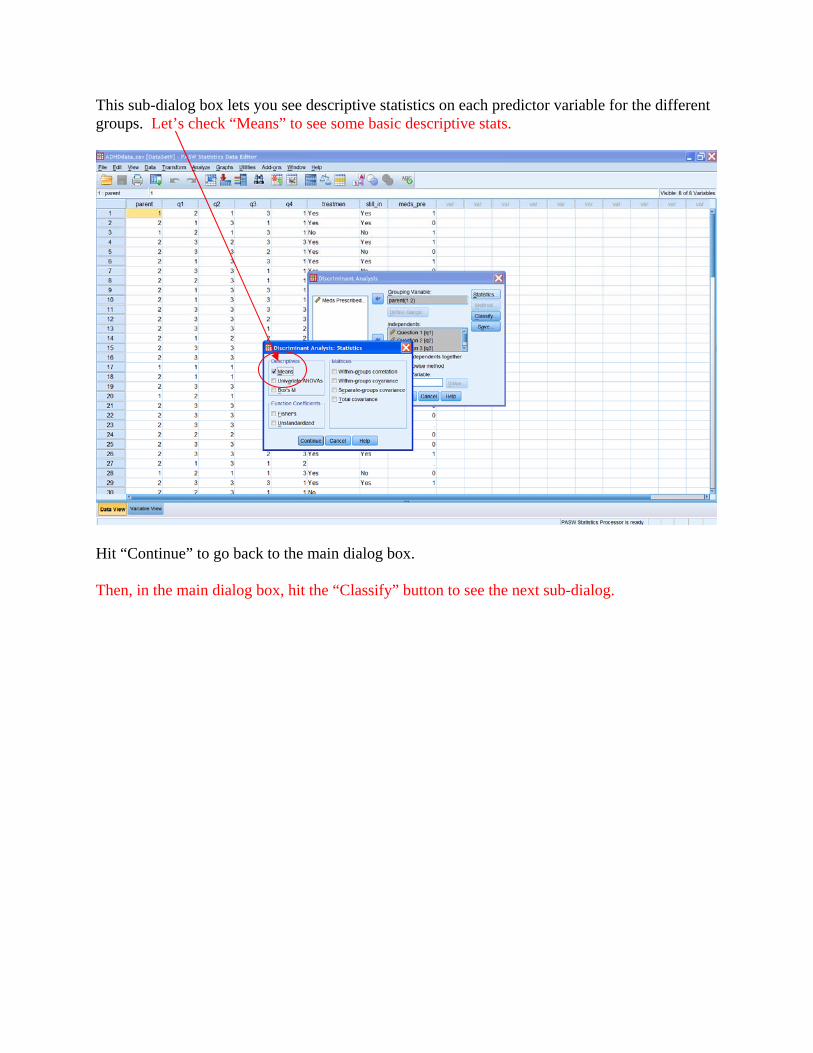
This sub-dialog box lets you see descriptive statistics on each predictor variable for the different groups. Let’s check “Means” to see some basic descriptive stats.

Hit “Continue” to go back to the main dialog box. Then, in the main dialog box, hit the “Classify” button to see the next sub-dialog.

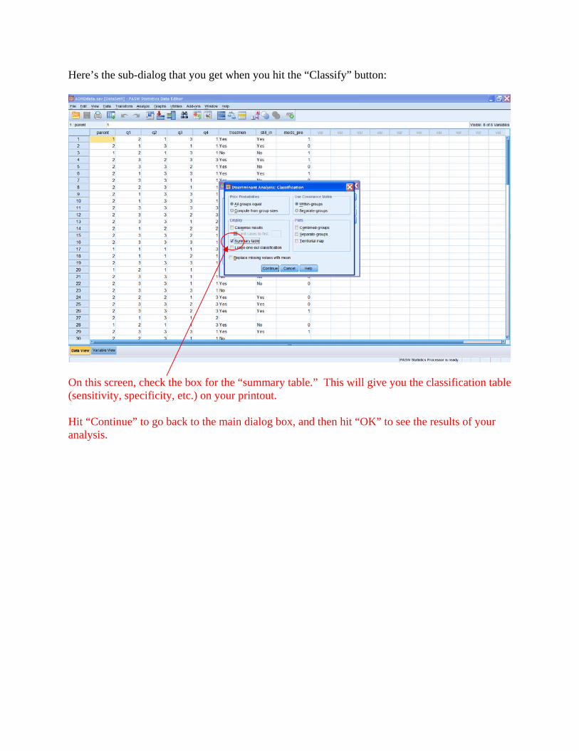
Here’s the sub-dialog that you get when you hit the “Classify” button:

On this screen, check the box for the “summary table.” This will give you the classification table (sensitivity, specificity, etc.) on your printout. Hit “Continue” to go back to the main dialog box, and then hit “OK” to see the results of your analysis.

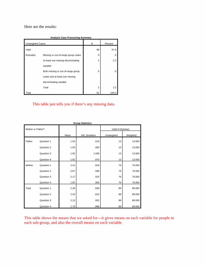
Here are the results:

Analysis Case Processing Summary

Unweighted Cases N Percent

Valid 89 97.8

Excluded Missing or out-of-range group codes 0 .0

At least one missing discriminating

variable

2 2.2

Both missing or out-of-range group

codes and at least one missing

discriminating variable

0 .0

Total 2 2.2

Total 91 100.0

This table just tells you if there’s any missing data.

Group Statistics

Mother or Father?

Mean Std. Deviation

Valid N (listwise)

Unweighted Weighted

Father Question 1 1.54 .519 13 13.000

Question 2 1.00 .000 13 13.000

Question 3 1.92 1.038 13 13.000

Question 4 1.62 .870 13 13.000

Mother Question 1 2.41 .819 76 76.000

Question 2 2.67 .598 76 76.000

Question 3 2.17 .915 76 76.000

Question 4 1.82 .905 76 76.000

Total Question 1 2.28 .839 89 89.000

Question 2 2.43 .810 89 89.000

Question 3 2.13 .932 89 89.000

Question 4 1.79 .898 89 89.000

This table shows the means that we asked for—it gives means on each variable for people in each sub-group, and also the overall means on each variable.

Summary of Canonical Discriminant Functions

Eigenvalues

Function

Eigenvalue % of Variance Cumulative %

Canonical

Correlation

dimension0 1 1.387a 100.0 100.0 .762

a. First 1 canonical discriminant functions were used in the analysis.

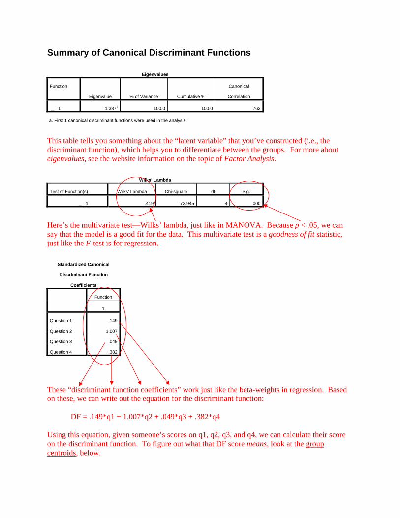
This table tells you something about the “latent variable” that you’ve constructed (i.e., the discriminant function), which helps you to differentiate between the groups. For more about eigenvalues, see the website information on the topic of Factor Analysis.

Wilks' Lambda

Test of Function(s) Wilks' Lambda Chi-square df Sig.

dimension0 1 .419 73.945 4 .000

Here’s the multivariate test—Wilks’ lambda, just like in MANOVA. Because p < .05, we can say that the model is a good fit for the data. This multivariate test is a goodness of fit statistic, just like the F-test is for regression.

Standardized Canonical

Discriminant Function

Coefficients

Function

1

Question 1 .149

Question 2 1.007

Question 3 .049

Question 4 .382

These “discriminant function coefficients” work just like the beta-weights in regression. Based on these, we can write out the equation for the discriminant function: DF = .149*q1 + 1.007*q2 + .049*q3 + .382*q4 Using this equation, given someone’s scores on q1, q2, q3, and q4, we can calculate their score on the discriminant function. To figure out what that DF score means, look at the group centroids, below.

Structure Matrix

Function

1

Question 2 .914

Question 1 .336

Question 3 .081

Question 4 .068

Pooled within-groups correlations

between discriminating variables

and standardized canonical

discriminant functions

Variables ordered by absolute

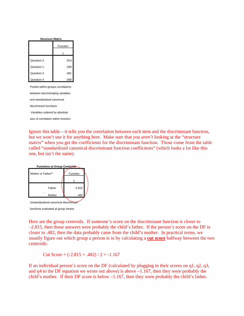
size of correlation within function. Ignore this table—it tells you the correlation between each item and the discriminant function, but we won’t use it for anything here. Make sure that you aren’t looking at the “structure matrix” when you get the coefficients for the discriminant function. Those come from the table called “standardized canonical discriminant function coefficients” (which looks a lot like this one, but isn’t the same).

Functions at Group Centroids

Mother or Father? Function

1

dimension0

Father -2.815

Mother .482

Unstandardized canonical discriminant

functions evaluated at group means Here are the group centroids. If someone’s score on the discriminant function is closer to –2.815, then those answers were probably the child’s father. If the person’s score on the DF is closer to .482, then the data probably came from the child’s mother. In practical terms, we usually figure out which group a person is in by calculating a cut score halfway between the two centroids: Cut Score = (-2.815 + .482) / 2 = -1.167 If an individual person’s score on the DF (calculated by plugging in their scores on q1, q2, q3, and q4 to the DF equation we wrote out above) is above –1.167, then they were probably the child’s mother. If their DF score is below –1.167, then they were probably the child’s father.

Classification Statistics

Classification Processing Summary

Processed 91

Excluded Missing or out-of-range group codes 0

At least one missing discriminating

variable

2

Used in Output 89

Prior Probabilities for Groups

Mother or Father?

Prior

Cases Used in Analysis

Unweighted Weighted

dimension0

Father .500 13 13.000

Mother .500 76 76.000

Total 1.000 89 89.000

Classification Resultsa

Mother or Father? Predicted Group Membership

Total Father Mother

Original Count dimension2

Father 13 0 13

Mother 6 70 76

% dimension2

Father 100.0 .0 100.0

Mother 7.9 92.1 100.0

a. 93.3% of original grouped cases correctly classified.

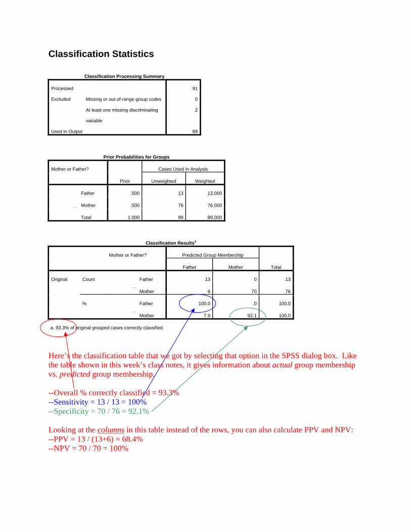
Here’s the classification table that we got by selecting that option in the SPSS dialog box. Like the table shown in this week’s class notes, it gives information about actual group membership vs. predicted group membership. --Overall % correctly classified = 93.3% --Sensitivity = 13 / 13 = 100% --Specificity = 70 / 76 = 92.1% Looking at the columns in this table instead of the rows, you can also calculate PPV and NPV: --PPV = 13 / (13+6) = 68.4% --NPV = 70 / 70 = 100%

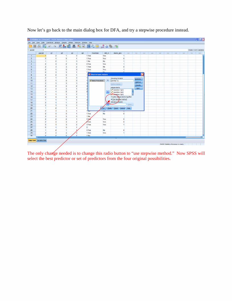
Now let’s go back to the main dialog box for DFA, and try a stepwise procedure instead.

The only change needed is to change this radio button to “use stepwise method.” Now SPSS will select the best predictor or set of predictors from the four original possibilities.

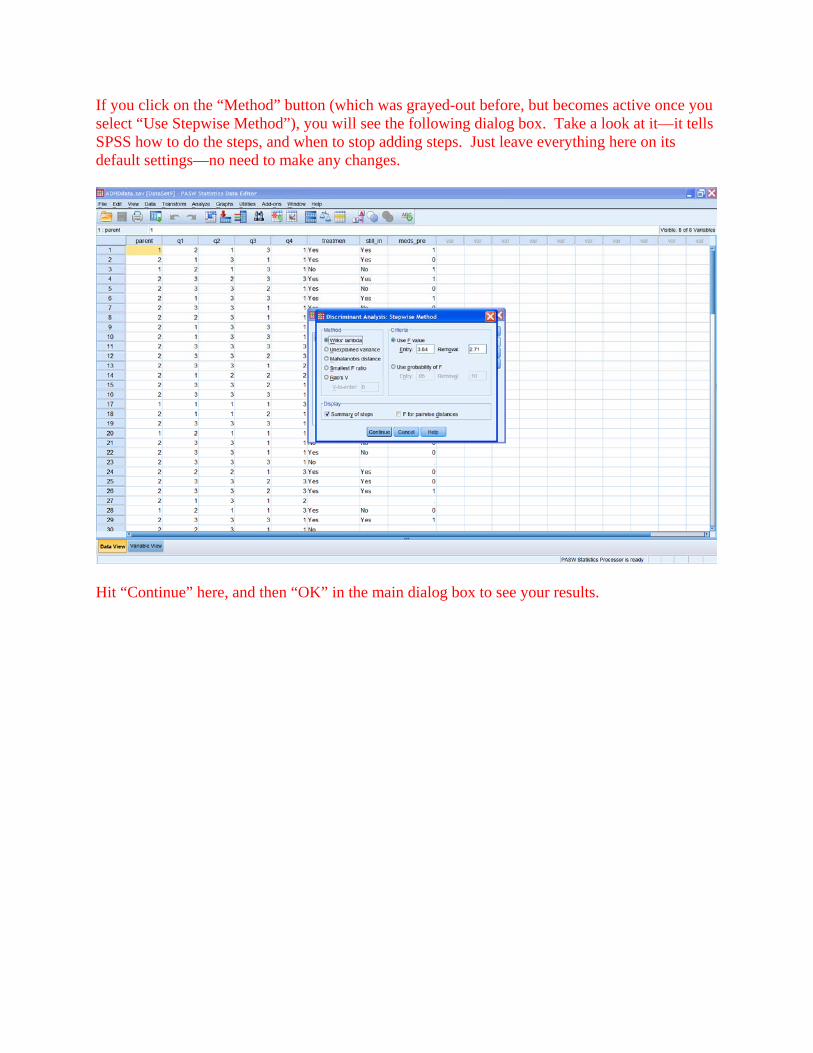
If you click on the “Method” button (which was grayed-out before, but becomes active once you select “Use Stepwise Method”), you will see the following dialog box. Take a look at it—it tells SPSS how to do the steps, and when to stop adding steps. Just leave everything here on its default settings—no need to make any changes.

Hit “Continue” here, and then “OK” in the main dialog box to see your results.

Discriminant [information omitted] Analysis 1 Stepwise Statistics

Variables Entered/Removeda,b,c,d

Step

Entered

Wilks' Lambda

Statistic df1 df2 df3

Exact F

Statistic df1 df2 Sig.

1 Question 2 .463 1 1 87.000 100.720 1 87.000 .000

2 Question 4 .426 2 1 87.000 58.050 2 86.000 .000

At each step, the variable that minimizes the overall Wilks' Lambda is entered.

a. Maximum number of steps is 8.

b. Minimum partial F to enter is 3.84.

c. Maximum partial F to remove is 2.71.

d. F level, tolerance, or VIN insufficient for further computation.

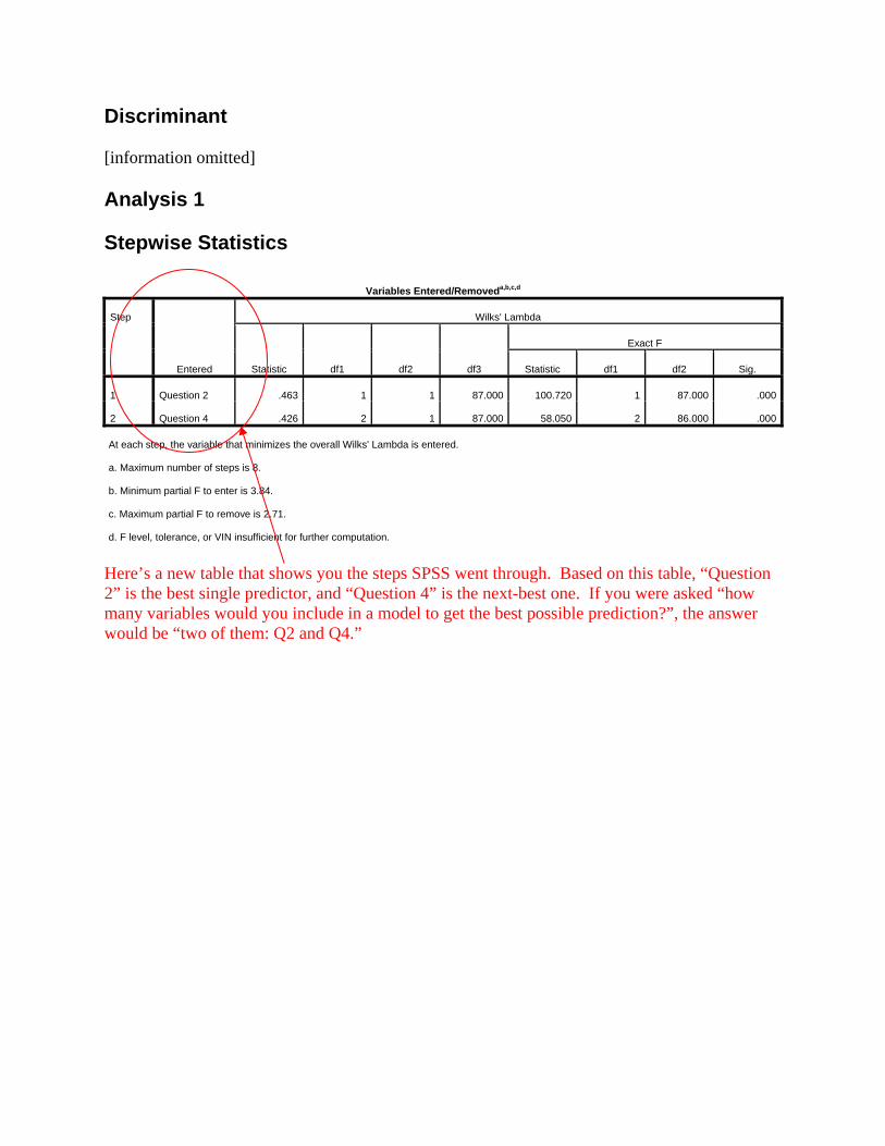
Here’s a new table that shows you the steps SPSS went through. Based on this table, “Question 2” is the best single predictor, and “Question 4” is the next-best one. If you were asked “how many variables would you include in a model to get the best possible prediction?”, the answer would be “two of them: Q2 and Q4.”

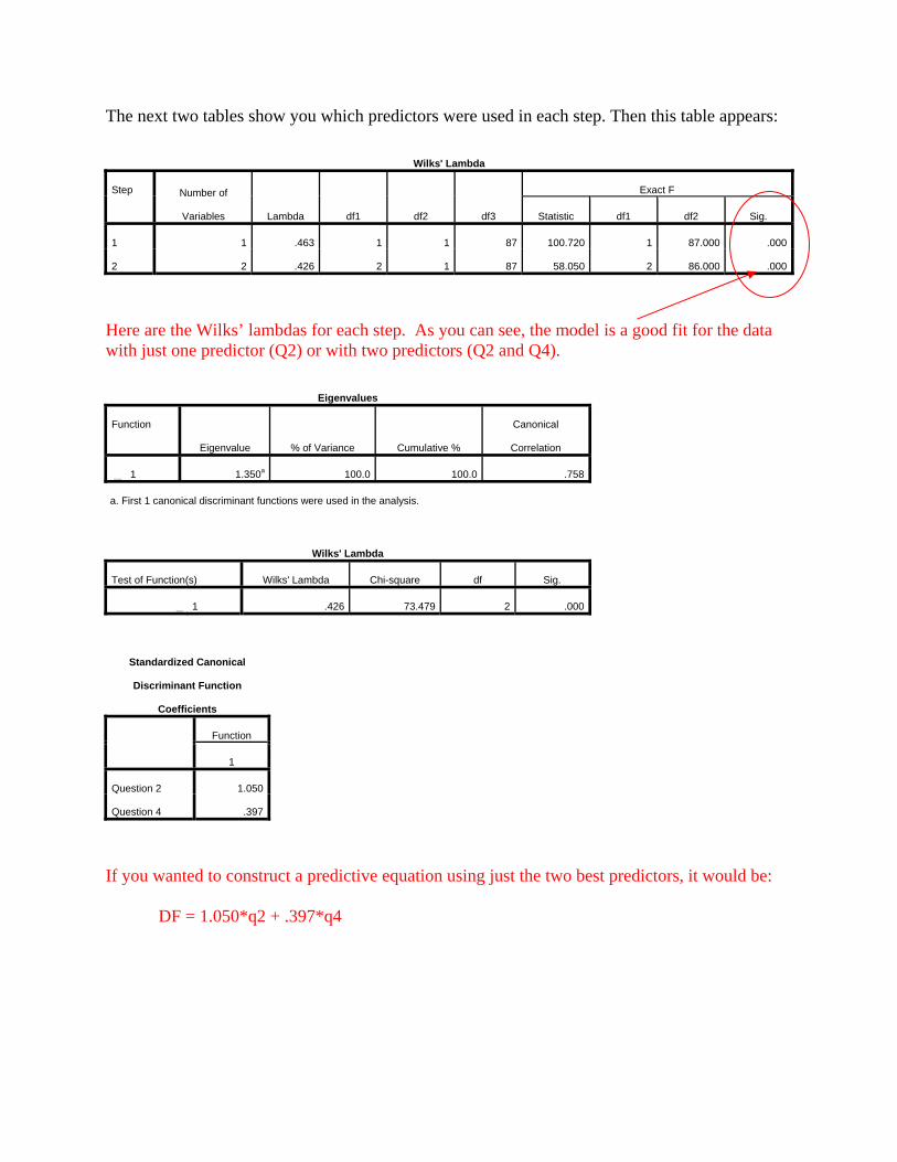
The next two tables show you which predictors were used in each step. Then this table appears:

Wilks' Lambda

Step Number of

Variables Lambda df1 df2 df3

Exact F

Statistic df1 df2 Sig.

1 1 .463 1 1 87 100.720 1 87.000 .000

2 2 .426 2 1 87 58.050 2 86.000 .000

Here are the Wilks’ lambdas for each step. As you can see, the model is a good fit for the data with just one predictor (Q2) or with two predictors (Q2 and Q4).

Eigenvalues

Function

Eigenvalue % of Variance Cumulative %

Canonical

Correlation

dimension0 1 1.350a 100.0 100.0 .758

a. First 1 canonical discriminant functions were used in the analysis.

Wilks' Lambda

Test of Function(s) Wilks' Lambda Chi-square df Sig.

dimension0 1 .426 73.479 2 .000

Standardized Canonical

Discriminant Function

Coefficients

Function

1

Question 2 1.050

Question 4 .397

If you wanted to construct a predictive equation using just the two best predictors, it would be: DF = 1.050*q2 + .397*q4

Structure Matrix

Function

1

Question 2 .926

Question 1a .186

Question 4 .068

Question 3a .003

Pooled within-groups correlations

between discriminating variables

and standardized canonical

discriminant functions

Variables ordered by absolute size

of correlation within function.

a. This variable not used in the

analysis.

Functions at Group Centroids

Mother or Father? Function

1

dimension0

Father -2.778

Mother .475

Unstandardized canonical discriminant

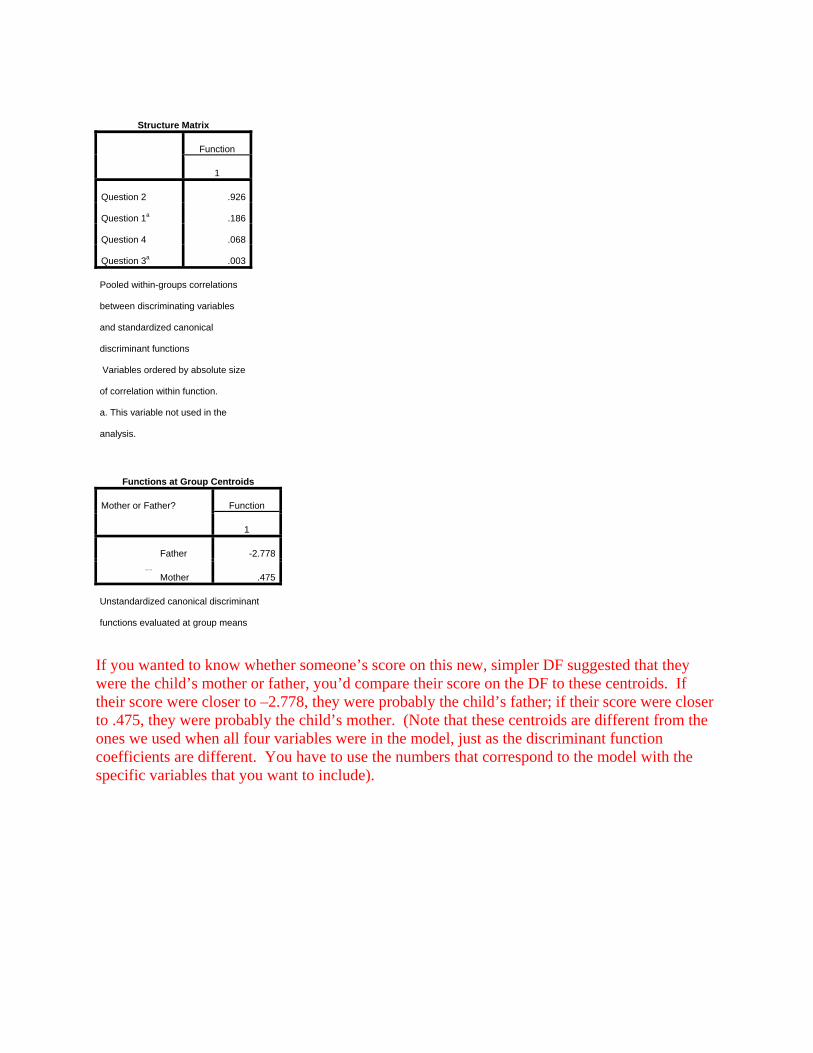
functions evaluated at group means If you wanted to know whether someone’s score on this new, simpler DF suggested that they were the child’s mother or father, you’d compare their score on the DF to these centroids. If their score were closer to –2.778, they were probably the child’s father; if their score were closer to .475, they were probably the child’s mother. (Note that these centroids are different from the ones we used when all four variables were in the model, just as the discriminant function coefficients are different. You have to use the numbers that correspond to the model with the specific variables that you want to include).

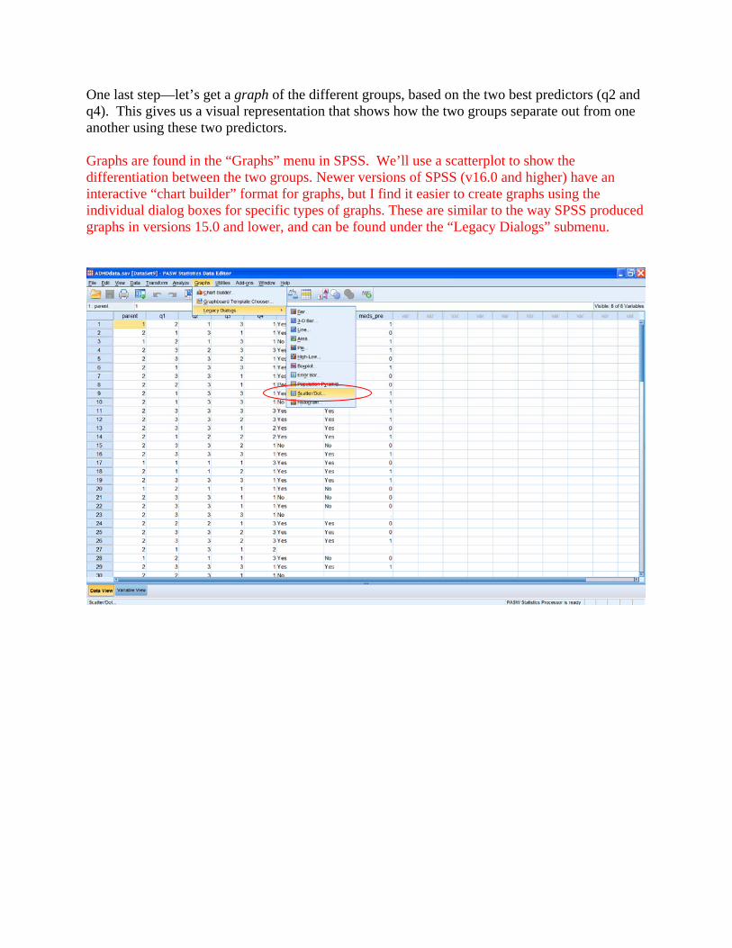
One last step—let’s get a graph of the different groups, based on the two best predictors (q2 and q4). This gives us a visual representation that shows how the two groups separate out from one another using these two predictors. Graphs are found in the “Graphs” menu in SPSS. We’ll use a scatterplot to show the differentiation between the two groups. Newer versions of SPSS (v16.0 and higher) have an interactive “chart builder” format for graphs, but I find it easier to create graphs using the individual dialog boxes for specific types of graphs. These are similar to the way SPSS produced graphs in versions 15.0 and lower, and can be found under the “Legacy Dialogs” submenu.

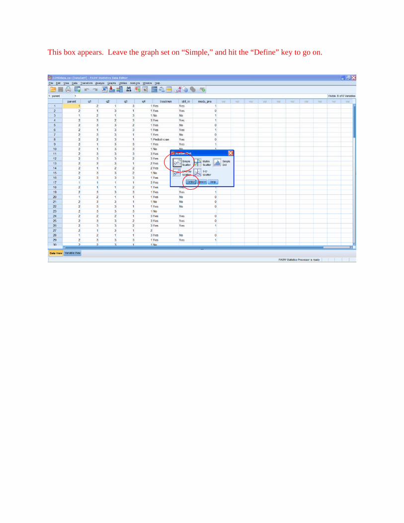
This box appears. Leave the graph set on “Simple,” and hit the “Define” key to go on.

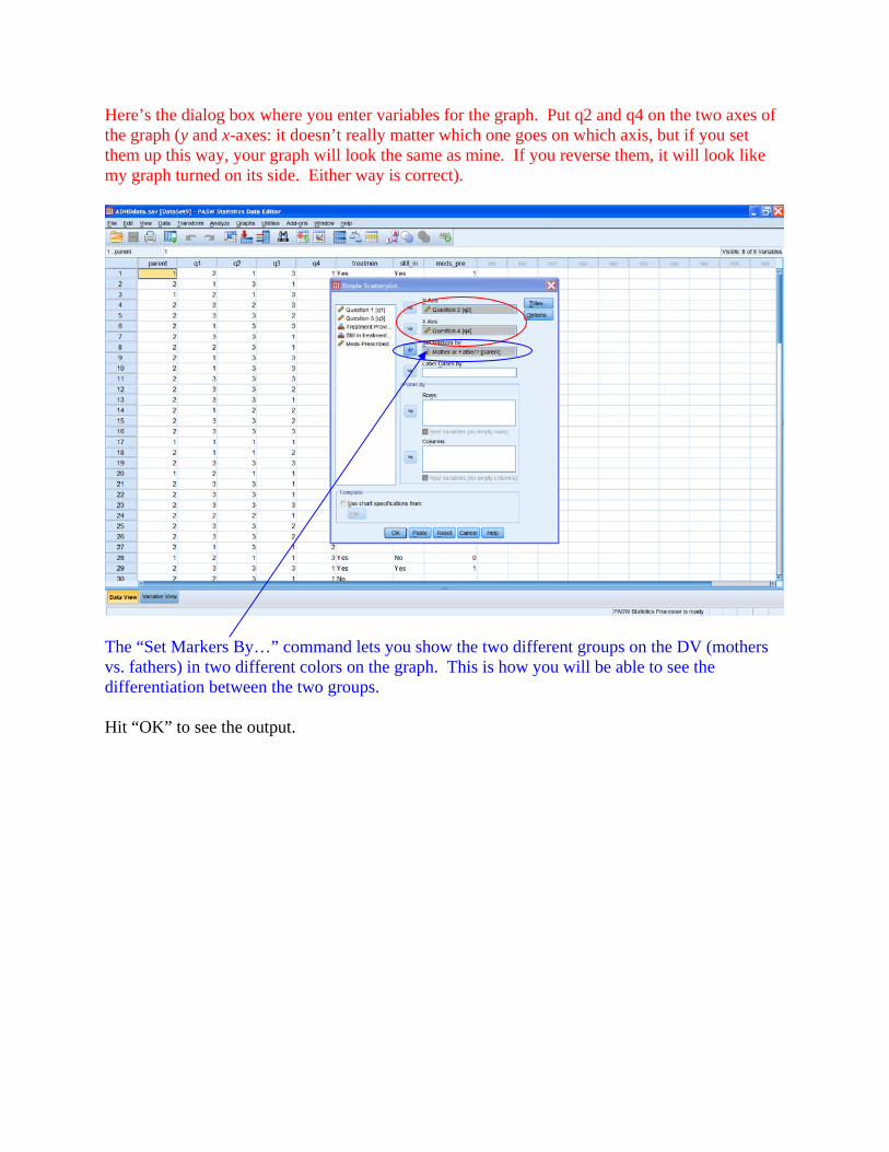
Here’s the dialog box where you enter variables for the graph. Put q2 and q4 on the two axes of the graph (y and x-axes: it doesn’t really matter which one goes on which axis, but if you set them up this way, your graph will look the same as mine. If you reverse them, it will look like my graph turned on its side. Either way is correct).

The “Set Markers By…” command lets you show the two different groups on the DV (mothers vs. fathers) in two different colors on the graph. This is how you will be able to see the differentiation between the two groups. Hit “OK” to see the output.

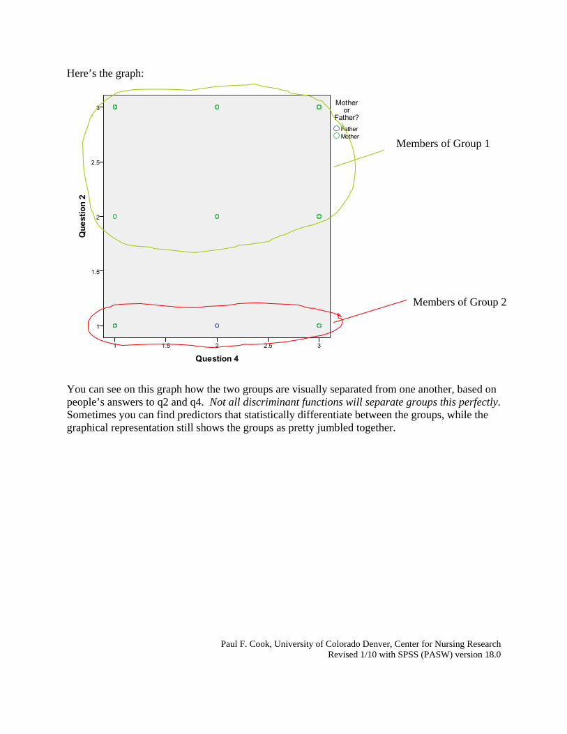
Here’s the graph:

You can see on this graph how the two groups are visually separated from one another, based on people’s answers to q2 and q4. Not all discriminant functions will separate groups this perfectly. Sometimes you can find predictors that statistically differentiate between the groups, while the graphical representation still shows the groups as pretty jumbled together.

Paul F. Cook, University of Colorado Denver, Center for Nursing Research Revised 1/10 with SPSS (PASW) version 18.0

Members of Group 1

Members of Group 2