Discretizing a Process with Non-zero Skewness and High ... · of a model depend crucially on this choice, calibrating the process and its discrete approximationdemandsgreatcare. Thankstotheirtractability,AR(1

Discretizing a Process with

Non-zero Skewness and High Kurtosis ∗

Simone Civale† Luis Díez-Catalán‡ Fatih Fazilet§

October 15, 2017

Abstract

We develop and test a discretization method to calibrate a Markov chain that

features non-zero skewness and high kurtosis. The proposed method applies the

logic of Tauchen (1986) to a first-order autoregressive process with normal mixture

innovations, which, as we discuss, can be calibrated to feature non-zero skewness

and high kurtosis. We then illustrate an application of our method in an Aiyagari

economy. We find that an idiosyncratic shock with higher kurtosis decreases the

equilibrium interest rate, whereas higher left skewness increases it.

JEL Code: C60

Keywords: Discretization method, skewness, kurtosis, non-Gaussian shocks, nor-

mal mixture, Markov chain.

1 Introduction

For many economic applications, researchers must specify a stochastic process thatgoverns the evolution of a key variable. Because the analytical and numerical solutions∗We are especially thankful for the guidance and feedback of Fatih Guvenen. We thank Anmol

Bhandari, Ellen McGrattan, Alessandro Peri, Georgios Stefanidis, Sergio Salgado, Matt Shapiro, andGuillaume Sublet for helpful comments and discussions.†Analysis Group, Inc. E-mail: [email protected]‡University of Minnesota. E-mail: [email protected]§University of Minnesota. E-mail: [email protected]

1

of a model depend crucially on this choice, calibrating the process and its discreteapproximation demands great care.

Thanks to their tractability, AR(1) processes with Gaussian innovations are a pop-ular choice for many problems in the literature. Consequently, several methods havebeen developed that can discretize an AR(1) process accurately.

However, a growing body of literature, including Bloom et al. (2012) and Guvenenet al. (2015), shows that higher order moments display interesting empirical patternsthat cannot be reproduced by a Gaussian AR(1) process. The analysis of these patternsposes a challenge for the economic practitioner who needs to choose (i) a process that istractable but flexible enough to capture these patterns and (ii) a discrete approximationof the process.

In this paper we develop and test a discretization method to calibrate a first-orderMarkov process that features non-zero skewness and excess kurtosis in the levels andin the innovations.

Since our discretization method is based on the method of Tauchen (1986) we willrefer to it as Extended Tauchen (ET). The ET method is different from the methodof Tauchen (1986) in two ways: (i) The innovations to the autoregressive process aredistributed as a mixture of normals. This assumption makes the process flexible enoughto feature the desired level of skewness and kurtosis. (ii) The choice of the state spaceis optimal with respect to a set of targeted moments. The latter change entails a sizablegain in the precision of the approximation.

In order to apply the ET method a practitioner needs to calibrate a first-orderautoregressive process with normal mixture innovations (NMAR). Therefore we studythe properties of a NMAR and uncover what combinations of skewness and kurtosisit can feature. We find that a NMAR is flexible enough to match the higher ordermoments found in the empirical literature.

Finally, we present an economic application of the Extended Tauchen method withina standard Aiyagari economy. We find that an increase in the kurtosis of the idiosyn-cratic shocks decreases the general equilibrium interest rate, while an increase in theleft skewness of the idiosyncratic shocks increases the equilibrium interest rate.

The rest of the paper is organized as follows. Section 2 illustrates the connection be-tween this paper and the existing literature. In Section 3 we discuss the calibration of aNMAR process and we study what combinations of skewness and kurtosis it can feature.

2

Section 4 introduces and tests the Extended Tauchen method. We show that ET canbe used to calibrate a discrete Markov chain that features non-Gaussian skewness andkurtosis. We then illustrate how accurately the method matches the values of skewnessand kurtosis found in the empirical literature. Finally, Section 5 presents an economicapplication of the Extended Tauchen method in a standard Aiyagari economy.

2 Related Literature

Because of their tractability, autoregressive processes with Gaussian innovations arewidely used to model key economic variables. Aiyagari (1994), Hubbard et al. (1995)and Storesletten et al. (2004) use an AR(1) process to model earning dynamics. Cooperand Haltiwanger (2006) use it to model the evolution of firm profits, while Arellano et al.(2012) employ it to model the dynamics of volatility.

To implement these frameworks numerically, several discretization methods exist toapproximate the continuous process with a Markov chain. Tauchen (1986) proposescalibrating the transition probabilities with the conditional distribution implied by theAR(1) process. Improving on this method, Tauchen and Hussey (1991) introduce theidea of placing the state space optimally. In fact, as they argue, the discretizationshould accurately approximate the integral equation that characterizes an economicproblem. They show that a quadrature rule describes the optimal placement.

The method of Rouwenhorst (1995) uses a simple construction to obtain a dis-crete Markov process that exactly matches the conditional and unconditional first twomoments and the autocorrelation of the process. This calibration offers a dramatic im-provement, especially in those applications where the persistence of the autoregressiveprocess is high1.

More closely related to this paper are Gospodinov and Lkhagvasuren (2014) andFarmer and Toda (2015). Gospodinov and Lkhagvasuren (2014) propose a calibrationmethod based on a moment matching procedure, and focuses on the calibration ofa multivariate VAR process. The authors also discuss a potential extension of theirmethod to calibrate a Markov Chain featuring non-zero skewness and excess kurtosis.However, they don’t explore the implementation of the method. Farmer and Toda

1Other related papers compare and establish the properties of these competing methods, oftenintroducing improvements or extensions as in Kopecky and Suen (2010), Galindev and Lkhagvasuren(2010), Adda and Cooper (2003), Flodén (2008) and Terry and Knotek II (2011).

3

(2015) develop a method to calibrate a discrete process that matches exactly a chosenset of conditional moments. However, this method can only be applied to processeswhose conditional moments can be matched exactly, which excludes most applicationswith non-zero skewness and high kurtosis.

More recently, a large body of literature has shown that higher order moments dis-play interesting empirical patterns, which can have major economic implications. In theliterature of earning dynamics, an early example is Geweke and Keane (1997), who fit anormal mixture model to earnings innovations using Panel Study of Income Dynamics(PSID) data. Guvenen et al. (2015), using US Social Security data, report that theinnovations to income are characterized by sizable skewness and high kurtosis. Bon-homme and Robin (2010) use PSID data to document excess kurtosis of the changesin earnings. Bloom et al. (2012) show that both the distribution of total factor pro-ductivity shocks and sales growth in the United States display negative skewness andexcess kurtosis. Bachmann et al. (2015) look at the higher order moments of investmentinnovations. They find sizable excess kurtosis but no significant skewness.

In the finance literature, several studies have documented that the returns on fi-nancial assets are leptokurtic—feature fat tails—and, in many cases, feature non-zeroskewness. An example is the early work of Mandelbrot (1963) and Fama (1965). Morerecent studies are, among others, Liu and Brorsen (1995) and Chiang and Li (2015).

In light of these findings, our study proposes how to specify a process that featuresnon-zero skewness and excess kurtosis, and provides a discretization tool to implementthe process numerically.

3 NMAR process

Several empirical studies have recently shown that the levels and the differences ofsome key economic variables display non-zero skewness and high kurtosis, which areimpossible to reproduce using an autoregressive process with Gaussian innovations. Inthis section we study a simple generalization of an AR(1) process that is flexible enoughto feature such skewness and kurtosis. We focus on a first-order autoregressive processwith normal mixture innovations (NMAR). The findings we discuss in this section areauxiliary to Section 4, since the Extended Tauchen method takes a calibrated NMARprocess as an input.

4

What motivates our choice is the simplicity and flexibility of this process. In factwe can easily characterize its moment structure and we can calibrate it to match a wideset of moments2. We then conclude the section illustrating the calibration of a NMARby targeting the income process moments found by Guvenen et al. (2015).

A NMAR process has the following representation:

yt = ρyt−1 + ηt, (1)

where

ηt ∼

{N(µ1, σ

21) with probability p1,

N(µ2, σ22) with probability p2,

and p2 = 1− p1. We denote ∆yt = yt − yt−1 and ∆kyt = yt − yt−k. In Appendix A1 wederive and report the mean, variance, skewness, and kurtosis of η, y and ∆ky. Thoughthese formulas are useful to calibrate the process and will be used in the followinganalysis, we don’t report them in the main body of the paper to keep it readable.

Inspecting Equation 9 and 10 we can see that the moments of y and ∆ky are de-termined by ρ and by the moments of η. To understand the trade-offs that theserelationships entail, we run a numerical experiment that studies what combinations of{Var(η), S(η),K(η)} are attainable.

In the first step of this exercise, we calibrate η using the Generalized Method ofMoments (GMM). We target combinations of Var(η) ∈ [0.1, 1], S(η) ∈ [−5, 0], andK(η) ∈ [3, 21]. The first important finding is that the feasibility of a {S(η),K(η)}combination is independent of Var(η). In light of this fact, we only discuss the feasiblecombinations of {S(η),K(η)}. In Figure 1 the feasible combinations of {S(η),K(η)} lienortheast (NE) of the blue line. In other words, there is a calibration of η that deliversexactly any combination {S(η),K(η)} in the NE region. The combinations southwest(SW) of the blue line can only be obtained with some error.

To understand the magnitude of this error we compute the average percentage dis-crepancy of the calibrated skewness and kurtosis from the target and we report it inFigure 1 using a grayscale. For example, the error associated with K(η) = 5 andS(η) = −3 is 20, meaning that the GMM calibration misses the targets of S and K byan average of 20%.

2Geweke and Keane (1997) and Kon (1984) among others have previously used this type of process.

5

Figure 1: Feasible combinations of {S(η),K(η)}In this figure we show what combinations of kurtosis, K(η), and skewness, S(η), are feasiblewhen calibrating a normal mixture η. The combinations NE of the blue line are exactlyattainable. For each {S(η),K(η)} in the SW region we report the average percentage absolutedeviation from {S(η),K(η)} using a grayscale.

To put Figure 1 in context, we report the combinations of {S(η),K(η)} found byBloom et al. (2012) and Bachmann et al. (2015), which we label B12 and B15, respec-tively. Both papers find combinations that are feasible under a NMAR3.

In the second step of this numerical exercise we map the feasible combinations{S(η),K(η)} into the feasible combinations of {S(∆y),K(∆y)} and {S(∆5y),K(∆5y)}.Since the mapping depends on the value of ρ, we repeat the exercise for ρ =

0.8, 0.9, 0.99.

In Figure 2 the feasible combinations of skewness and kurtosis lie NE of each frontier.To put this figure in context, we report the combinations of skewness and kurtosisfound by Bloom et al. (2012) and Guvenen et al. (2015), which we label B12 and G15,respectively. Both papers find combinations that are feasible under NMAR for theselected values of ρ4.

In the remaining part of this section we consider an application. We calibrate aNMAR process with GMM, targeting the data moments of Guvenen et al. (2015), which

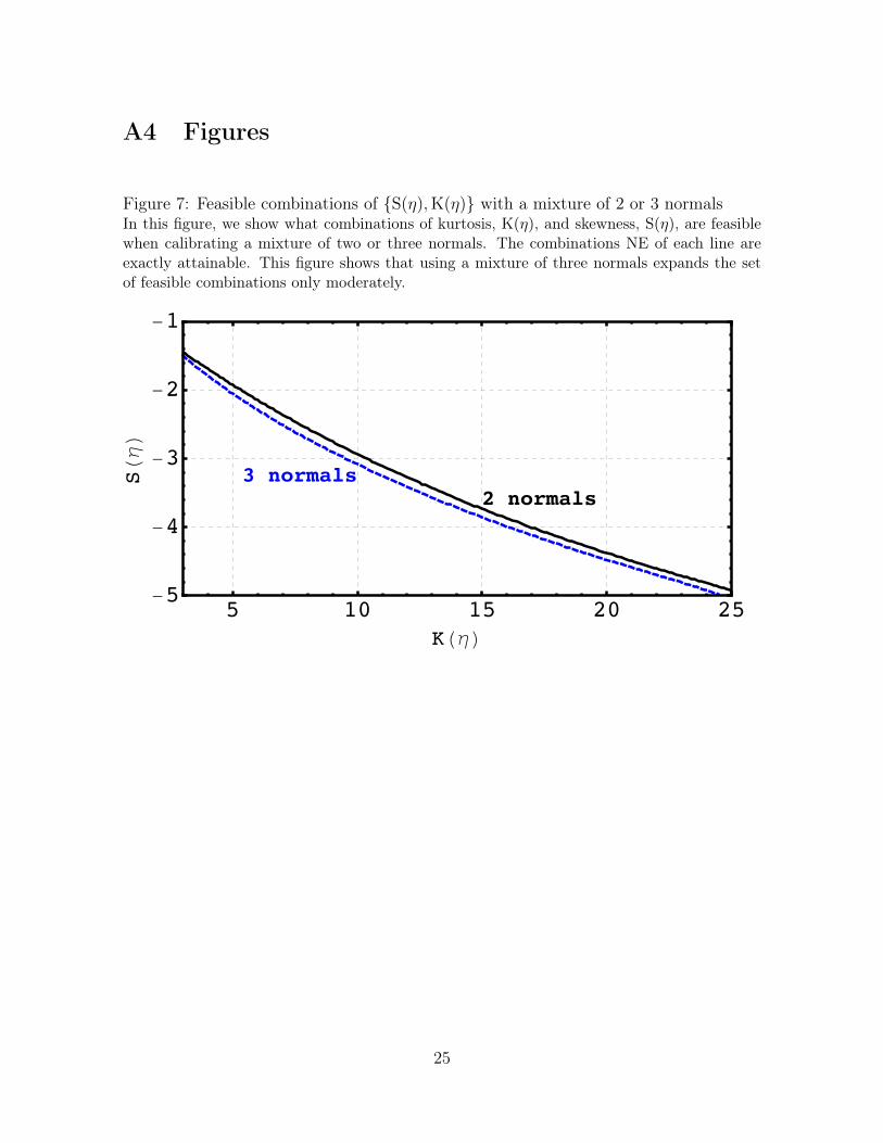
3In Figure 7, we repeat this first step of the numerical exercise to understand what is gained fromusing a mixture of three normals rather than two normals.

4As Equation 10 shows ρ and the moments of η pin down the lag-profile of skewness and kurtosisof the process. This establishes some trade-offs that we explore in the Online Appendix.

6

Figure 2: Feasible combinations of {S(∆y),K(∆y)} and {S(∆5y),K(∆5y)}In this figure we show what combinations of {S(∆y),K(∆y)} and {S(∆5y),K(∆5y)} are ex-actly attainable when calibrating a NMAR process. Within each quadrant we draw the frontierfor three different values of ρ. The feasible combinations lie NE of each frontier.

�(Δ�)

ρ=�� ρ=�� ρ=��

��◼

◼

� �� -�

-�

-�

-�

�

�(Δ�)

�(Δ��)

ρ=��

ρ=��

ρ=��

��◼◼

� �� -�

-�

-�

-�

�

�(Δ� �)

we report in Table 1. Six parameters (ρ, p1, µ1, µ2, σ1, σ2) govern NMAR with two nor-mals. The strategy we follow sets ρ = 0.99, p1 = 0.9, and imposes µ2 = −p1µ1/ (1− p1)

to ensure that E (η) = 0. This leaves 3 parameters to calibrate, (µ1, σ1, σ2). Table 2reports the parametrization of the NMAR that yields exactly the moments targetedin Table 1, and in Table 3 we report the complete moment structure of the calibratedprocess.

Table 1: Targeted data moments

E(∆y) Var(∆y) S(∆y) K(∆y)0 0.23 -1.35 17.8

Table 2: NMAR calibration

µ1 µ2 σ21 σ2

2 p1

0.0336 -0.3021 0.0574 1.6749 0.9000

Table 3: Moments of the calibrated process

E(ηt) = 0 E(yt) = 0 E(∆yt) = 0Var(ηt) = 0.23 Var(yt) = 11.50 Var(∆yt) = 0.23S(ηt) = −1.36 S(yt) = −0.12 S(∆yt) = −1.35K(ηt) = 17.95 K(yt) = 3.15 K(∆yt) = 17.80

7

4 Extended Tauchen Method

In this section we propose and discuss the Extended Tauchen (ET) method, whichconsists of a procedure to discretize a NMAR process. Though the calibration of thetransition probabilities follows the method of Tauchen (1986), ET differs from it in twoimportant ways. First, we discretize a NMAR instead of a Gaussian AR(1) process,therefore allowing the discrete process to feature non-zero skewness and high kurtosis.Second, the placement of the state space is chosen optimally with respect to a set oftargeted moments. This allows a sizable gain in the precision of the approximation.

In Section 3 we show that a NMAR process is flexible enough to feature non-zeroskewness and high kurtosis. We also illustrate how to calibrate NMAR using incomedata moments. In this section, we explore how to discretize a NMAR process specifiedas in Equation 1 and parametrized by θ = (ρ, p1, µ1, µ2, σ1, σ2).

The objective of the procedure is to calibrate a Markov chain, which we denote by(z, T ), where z is a state vector and T is a transition matrix. To apply this method apractitioner needs to choose a set of target moments. This choice needs to be based onwhat moments of the process are relevant for the specific application.

Let m (θ) denote a mapping from the continuous process into the set of relevantmoments and m̂ (z, T ) a mapping of (z, T ) into the same set of moments. The practi-tioner also needs to choose a notion of distance between the targets and the momentsof the Markov chain. We denote this distance by |m (θ)− m̂ (z, T )|, shorthand for[m (θ)− m̂ (z, T )]′W [m (θ)− m̂ (z, T )], where W is a weighting matrix. Finally, wewill denote by F the cumulative distribution function of η.

The method we propose has the following steps:

1. Choose the number of states n for the discrete process.

2. Choose a grid of states z = z1, . . . , zn of dimension n.

3. Compute n+ 1 nodes d = d1, . . . , dn+1 as

di =

−∞ if i = 1

∞ if i = n+ 1

(zi−1 + zi) /2 otherwise.

8

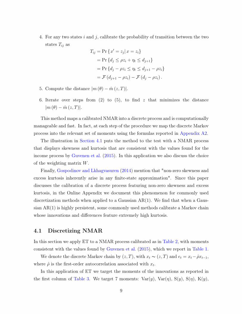
4. For any two states i and j, calibrate the probability of transition between the twostates Tij as

Tij = Pr {x′ = zj|x = zi}

= Pr {dj ≤ ρzi + ηt ≤ dj+1}

= Pr {dj − ρzi ≤ ηt ≤ dj+1 − ρzi}

= F (dj+1 − ρzi)−F (dj − ρzi) .

5. Compute the distance |m (θ)− m̂ (z, T )|.

6. Iterate over steps from (2) to (5), to find z that minimizes the distance|m (θ)− m̂ (z, T )|.

This method maps a calibrated NMAR into a discrete process and is computationallymanageable and fast. In fact, at each step of the procedure we map the discrete Markovprocess into the relevant set of moments using the formulas reported in Appendix A2.

The illustration in Section 4.1 puts the method to the test with a NMAR processthat displays skewness and kurtosis that are consistent with the values found for theincome process by Guvenen et al. (2015). In this application we also discuss the choiceof the weighting matrix W .

Finally, Gospodinov and Lkhagvasuren (2014) mention that "non-zero skewness andexcess kurtosis inherently arise in any finite-state approximation". Since this paperdiscusses the calibration of a discrete process featuring non-zero skewness and excesskurtosis, in the Online Appendix we document this phenomenon for commonly useddiscretization methods when applied to a Gaussian AR(1). We find that when a Gaus-sian AR(1) is highly persistent, some commonly used methods calibrate a Markov chainwhose innovations and differences feature extremely high kurtosis.

4.1 Discretizing NMAR

In this section we apply ET to a NMAR process calibrated as in Table 2, with momentsconsistent with the values found by Guvenen et al. (2015), which we report in Table 1.

We denote the discrete Markov chain by (z, T ), with xt ∼ (z, T ) and et = xt− ρ̂xt−1,where ρ̂ is the first-order autocorrelation associated with xt.

In this application of ET we target the moments of the innovations as reported inthe first column of Table 3. We target 7 moments: Var(y), Var(η), S(y), S(η), K(y),

9

K(η), and ρ. Since one can always adjust the state space to match the mean of theprocess, we don’t target it.

For this application we choose the weighting matrix so that |m (θ)− m̂ (z, T )| isequal to the sum of squared percentage deviations of each moment from its target.With this choice of W the deviations are expressed as a percentage—therefore scaleindependent—and each percentage moment condition is weighted equally. Since thechoice of W entails a precision trade-off between the targets it can only be refined inlight of a specific application.

Table 4 shows the results from the calibration5. For ease of interpretation, we reportthe average percentage absolute deviation of the moments from the targets. We repeatthe exercise for ρ = 0.5, 0.9, 0.95, 0.99, and N = 5, 9, 15, 19.

We observe that the performance improves with the number of states and that amore persistent process is calibrated less accurately. In Appendix A3 we discuss thecomputational tractability of this method.

Figure 3 concludes this application by plotting the histogram of the stationarydistributions of the innovations and of the levels of the calibrated process for ρ = 0.95

and for N = 9, 19. This figures illustrate how the innovations and the levels of theprocess are leptokurtic and left-skewed.

5 Aiyagari Calibrated with Extended Tauchen

In this section, we illustrate an application of the ET method in an Aiyagari (1994)economy. The household problem is

max.{ct,at+1}

E0

∞∑t=0

βtc1−µt

1− µ

s.t. ct + at+1 = (1 + r)at + wlt

(2)

where at+1 ≥ 0. The log-labor endowment follows a NMAR process. We calibrate thediscrete process for labor endowment with 15 states to feature non-zero skewness andhigh kurtosis, and we observe the implications of the higher order moments in generalequilibrium.

5We also target the moments found in Bloom et al. (2012) and Bachmann et al. (2015). We onlyreport the results for Guvenen et al. (2015) because they are the furthest from the normal case, andtherefore the most difficult to accurately match.

10

Figure 3: Extended Tauchen, NMARThis figure displays the histogram of the innovations, that is, Eij = zj − ρ(x)zi, and thehistogram of the levels x implied by a Markov chain calibrated with the Extended Tauchenmethod. In this example, ρ = 0.95, and we report the results for 9 and 19 states. Noticethat in the first and third panel of this figure, we rescale the y-axis by applying a cubic roottransformation in order to make the tails of the distribution conspicuous.

Eij

-5 -2.5 0 2.5 5

0.010.1

0.5 Var(2) = 0.23 S(2) = -1.36 K(2) = 17.95

Innovations, ;=0.95, N=9

zi

-5 -2.5 0 2.5 50.03

0.14

0.25 Var(y) = 2.36 S(y) = -0.30 K(y) = 3.77

Levels, ;=0.95, N=9

Eij

-5 -2.5 0 2.5 5

0.010.1

0.5

Innovations, ;=0.95, N=19

zi

-5 -2.5 0 2.5 50.02

0.08

0.14Levels, ;=0.95, N=19

11

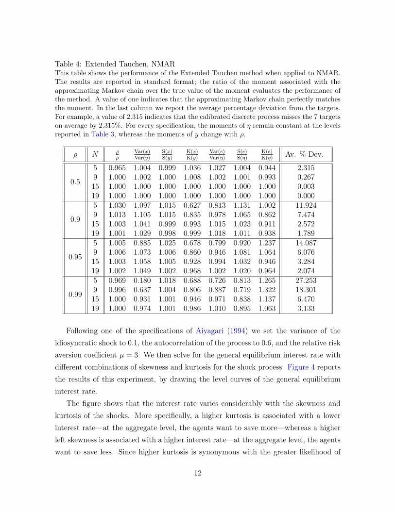
Table 4: Extended Tauchen, NMARThis table shows the performance of the Extended Tauchen method when applied to NMAR.The results are reported in standard format; the ratio of the moment associated with theapproximating Markov chain over the true value of the moment evaluates the performance ofthe method. A value of one indicates that the approximating Markov chain perfectly matchesthe moment. In the last column we report the average percentage deviation from the targets.For example, a value of 2.315 indicates that the calibrated discrete process misses the 7 targetson average by 2.315%. For every specification, the moments of η remain constant at the levelsreported in Table 3, whereas the moments of y change with ρ.

ρ N ρ̂ρ

Var(x)Var(y)

S(x)S(y)

K(x)K(y)

Var(e)Var(η)

S(e)S(η)

K(e)K(η)

Av. % Dev.

0.5

5 0.965 1.004 0.999 1.036 1.027 1.004 0.944 2.3159 1.000 1.002 1.000 1.008 1.002 1.001 0.993 0.26715 1.000 1.000 1.000 1.000 1.000 1.000 1.000 0.00319 1.000 1.000 1.000 1.000 1.000 1.000 1.000 0.000

0.9

5 1.030 1.097 1.015 0.627 0.813 1.131 1.002 11.9249 1.013 1.105 1.015 0.835 0.978 1.065 0.862 7.47415 1.003 1.041 0.999 0.993 1.015 1.023 0.911 2.57219 1.001 1.029 0.998 0.999 1.018 1.011 0.938 1.789

0.95

5 1.005 0.885 1.025 0.678 0.799 0.920 1.237 14.0879 1.006 1.073 1.006 0.860 0.946 1.081 1.064 6.07615 1.003 1.058 1.005 0.928 0.994 1.032 0.946 3.28419 1.002 1.049 1.002 0.968 1.002 1.020 0.964 2.074

0.99

5 0.969 0.180 1.018 0.688 0.726 0.813 1.265 27.2539 0.996 0.637 1.004 0.806 0.887 0.719 1.322 18.30115 1.000 0.931 1.001 0.946 0.971 0.838 1.137 6.47019 1.000 0.974 1.001 0.986 1.010 0.895 1.063 3.133

Following one of the specifications of Aiyagari (1994) we set the variance of theidiosyncratic shock to 0.1, the autocorrelation of the process to 0.6, and the relative riskaversion coefficient µ = 3. We then solve for the general equilibrium interest rate withdifferent combinations of skewness and kurtosis for the shock process. Figure 4 reportsthe results of this experiment, by drawing the level curves of the general equilibriuminterest rate.

The figure shows that the interest rate varies considerably with the skewness andkurtosis of the shocks. More specifically, a higher kurtosis is associated with a lowerinterest rate—at the aggregate level, the agents want to save more—whereas a higherleft skewness is associated with a higher interest rate—at the aggregate level, the agentswant to save less. Since higher kurtosis is synonymous with the greater likelihood of

12

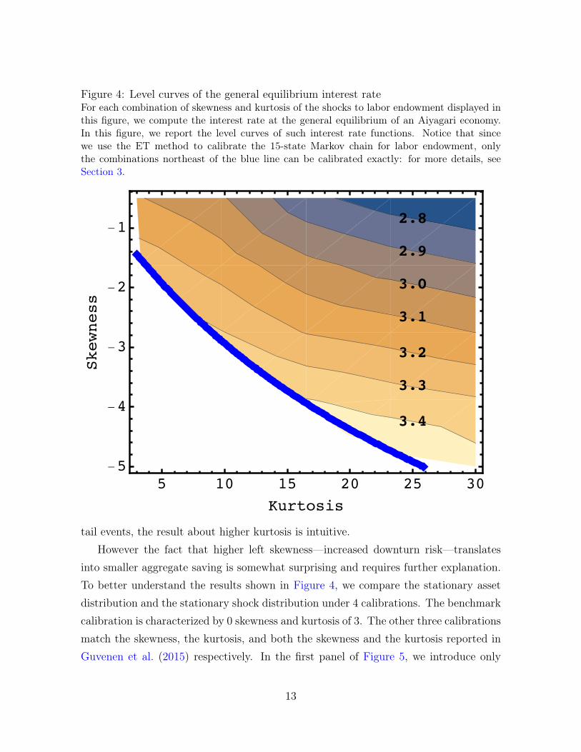
Figure 4: Level curves of the general equilibrium interest rateFor each combination of skewness and kurtosis of the shocks to labor endowment displayed inthis figure, we compute the interest rate at the general equilibrium of an Aiyagari economy.In this figure, we report the level curves of such interest rate functions. Notice that sincewe use the ET method to calibrate the 15-state Markov chain for labor endowment, onlythe combinations northeast of the blue line can be calibrated exactly: for more details, seeSection 3.

��

��

��

��

��

��

��

� �� -�

-�

-�

-�

-�

��

��

tail events, the result about higher kurtosis is intuitive.However the fact that higher left skewness—increased downturn risk—translates

into smaller aggregate saving is somewhat surprising and requires further explanation.To better understand the results shown in Figure 4, we compare the stationary assetdistribution and the stationary shock distribution under 4 calibrations. The benchmarkcalibration is characterized by 0 skewness and kurtosis of 3. The other three calibrationsmatch the skewness, the kurtosis, and both the skewness and the kurtosis reported inGuvenen et al. (2015) respectively. In the first panel of Figure 5, we introduce only

13

skewness and we observe that the agents who are close to the borrowing constraint savemore whereas wealthier agents save less. Because the effect on the upper tail dominatesthe effect on the left shoulder of the distribution, aggregate saving decreases and theinterest rate increases. By comparing the first and second panel of Figure 6, we cangain some intuition into why wealthier agents save less under a process with higherleft skewness. We observe that matching negative skewness while keeping the othermoments of the distribution constant means that some probability mass must moveabove zero. In fact under a process with negative skewness of -1.36 the probability ofa positive shock is 0.57 as opposed to 0.40 under the benchmark case. Since wealthyagents are not sensitive to left skewness but face a higher probability of receiving agood shock they save less.

In the second panel of Figure 5, we introduce only kurtosis, which results in higheraggregate saving. In the third panel, we introduce both skewness and kurtosis. Since theeffect of kurtosis dominates the effect of skewness, aggregate saving increases. Becausethe two effects tend to cancel each other out, the change in interest rate is only moderate,even though the change in the asset distributions is sizable.

6 Conclusion

The main contribution of this paper is to provide a discretization method to calibratea Markov chain that features non-zero skewness and high kurtosis.

The Extended Tauchen method calibrates a Markov chain using a procedure thatis similar to that of Tauchen (1986). This method is fast and delivers an accuratecalibration.

Finally, we illustrate an economic application of the Extended Tauchen method inan Aiyagari economy. We find that introducing idiosyncratic shocks with skewnessand excess kurtosis affects the aggregate level of savings and its distribution, thereforechanging the general equilibrium interest rate.

14

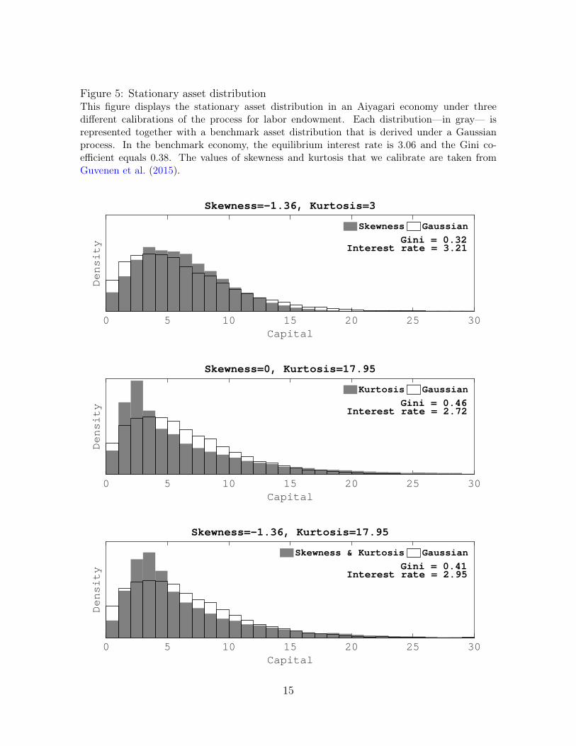
Figure 5: Stationary asset distributionThis figure displays the stationary asset distribution in an Aiyagari economy under threedifferent calibrations of the process for labor endowment. Each distribution—in gray— isrepresented together with a benchmark asset distribution that is derived under a Gaussianprocess. In the benchmark economy, the equilibrium interest rate is 3.06 and the Gini co-efficient equals 0.38. The values of skewness and kurtosis that we calibrate are taken fromGuvenen et al. (2015).

Capital0 5 10 15 20 25 30

Density Interest rate = 3.21

Gini = 0.32

Skewness=-1.36, Kurtosis=3

Skewness Gaussian

Capital0 5 10 15 20 25 30


Gini = 0.46

Skewness=0, Kurtosis=17.95

Kurtosis Gaussian

Capital0 5 10 15 20 25 30


Gini = 0.41

Skewness=-1.36, Kurtosis=17.95

Skewness & Kurtosis Gaussian

15

Figure 6: Stationary distribution of labor endowmentThis figure displays the stationary distribution of the levels of labor endowments under fourdifferent calibrations. The values of skewness and kurtosis that we calibrate are taken fromGuvenen et al. (2015).

zi

-2.5 0 2.5

0.1

0.2

Skewness=0, Kurtosis=3

zi

-2.5 0 2.5

0.1

Skewness=-1.36, Kurtosis=3

zi

-2.5 0 2.5

0.1

0.2

Skewness=0, Kurtosis=17.95

zi

-2.5 0 2.5

0.1

0.2

Skewness=-1.36, Kurtosis=17.95

16

References

Adda, J. and Cooper, R. W. (2003). Dynamic Economics: Quantitative Methods andApplications. MIT Press.

Aiyagari, S. R. (1994). Uninsured Idiosyncratic Risk and Aggregate Saving. QuarterlyJournal of Economics, 109(3):659–684.

Arellano, C., Bai, Y., and Kehoe, P. J. (2012). Financial Frictions and Fluctuations inVolatility. Technical report.

Bachmann, R., Elstner, S., and Hristov, A. (2015). Surprise, Surprise—MeasuringFirm-Level Investment Innovations.

Bloom, N., Floetotto, M., Jaimovich, N., Saporta-Eksten, I., and Terry, S. J. (2012).Really uncertain business cycles. (18245).

Bonhomme, S. and Robin, J.-M. (2010). Generalized Non-Parametric Deconvolutionwith an Application to Earnings Dynamics. Review of Economic Studies, 77(2):491–533.

Chiang, T. and Li, J. (2015). Modeling asset returns with skewness, kurtosis, andoutliers. Technical report.

Cooper, R. W. and Haltiwanger, J. C. (2006). On the Nature of Capital AdjustmentCosts. Review of Economic Studies, 73(3):611–633.

Fama, E. F. (1965). The behaviour of stock market prices. Journal of Business,38(1):34–105.

Farmer, L. E. and Toda, A. A. (2015). Discretizing Stochastic Processes with ExactConditional Moments.

Flodén, M. (2008). A Note on the Accuracy of Markov-Chain Approximations to HighlyPersistent AR(1) Processes. Economics Letters, 99(3):516–520.

Galindev, R. and Lkhagvasuren, D. (2010). Discretization of Highly Persistent Corre-lated AR(1) Shocks. Journal of Economic Dynamics and Control, 34(7):1260–1276.

17

Geweke, J. F. and Keane, M. P. (1997). An Empirical Analysis of Income DynamicsAmong Men in the PSID: 1968-1989. (233).

Gospodinov, N. and Lkhagvasuren, D. (2014). A Moment Matching Method for Ap-proximating Vector Autoregressive Processes by Finite State Markov Chains. Journalof Applied Econometrics, 29(5):843–859.

Guvenen, F. (2017). Quantitative Economics With Heterogeneity: An A-to-Z Guide-book.

Guvenen, F., Karahan, F., Ozkan, S., and Song, J. (2015). What Do Data on Millionsof U.S. Workers Reveal about Life-Cycle Earnings Risk? (20913).

Hubbard, R. G., Skinner, J., and Zeldes, S. P. (1995). Precautionary Saving and SocialInsurance. Journal of Political Economy, 103(2):360–399.

Kon, S. J. (1984). Models of Stock Returns—A Comparison. Journal of Finance,39(1):147–165.

Kopecky, K. and Suen, R. (2010). Finite State Markov-Chain Approximations to HighlyPersistent Processes. Review of Economic Dynamics, 13(3):701–714.

Liu, S.-M. and Brorsen, B. W. (1995). Maximum Likelihood Estimation of a GARCH-Stable Model. Journal of Applied Econometrics, 10(3):273–85.

Mandelbrot, B. (1963). The Variation of Certain Speculative Prices. Journal of Busi-ness, 36:394.

Rouwenhorst, G. K. (1995). Asset pricing implications of equilibrium business cyclemodels. In Frontiers of Business Cycle Research. Princeton University Press.

Storesletten, K., Telmer, C. I., and Yaron, A. (2004). Consumption and Risk SharingOver the Life Cycle. Journal of Monetary Economics, 51(3):609–633.

Tauchen, G. (1986). Finite State Markov-Chain Approximations to Univariate andVector Autoregressions. Economics Letters, 20(2):177–181.

Tauchen, G. and Hussey, R. (1991). Quadrature-Based Methods for Obtaining Approx-imate Solutions to Nonlinear Asset Pricing Models. Econometrica, 59(2):371–96.

18

Terry, S. J. and Knotek II, E. S. (2011). Markov-Chain Approximations of Vector Au-toregressions: Application of General Multivariate-Normal Integration Techniques.Economics Letters, 110(1):4–6.

APPENDIX

A1 Moments of NMAR

Consider a NMAR process with the following representation: yt = ρyt+1 + ηt, where

ηt =

{η1 ∼ N(µ1, σ


η2 ∼ N(µ2, σ22) with probability p2.

and ρ < 1. In order to calculate the moments of this process, we use the followingproperties. First, the raw moments of the innovation can be computed as a weightedsum of the raw moments of each of the normals: E(ηr) = p1E(ηr1) + p2E(ηr2). Second,to calculate the moments of yt, and ∆kyt, we use some properties of cumulants. (i)The nth cumulant of a distribution is homogeneous of degree n, which means thatCn(aX) = anC(X). (ii) Cumulants are additive, so that if X and Y are independentrandom variables, then Cn(X + Y ) = Cn(X) +Cn(Y ). (iii) The following relationshipshold.

C1(X) = E(X), C2(X) = Var(X),

C3(X) = S(X)Var(X)3/2, C4(X) = K(X)Var(X)2 − 3Var(X)2.(3)

Since

yt =∞∑h=0

ηt−hρh,

then∆kyt = yt − yt−k,

=∞∑h=0

ηt−hρh −

∞∑h=0

ηt−k−hρh,

=k−1∑h=0

ηt−hρh +

(1− ρ−k

) ∞∑h=k

ηt−hρh.

(4)

19

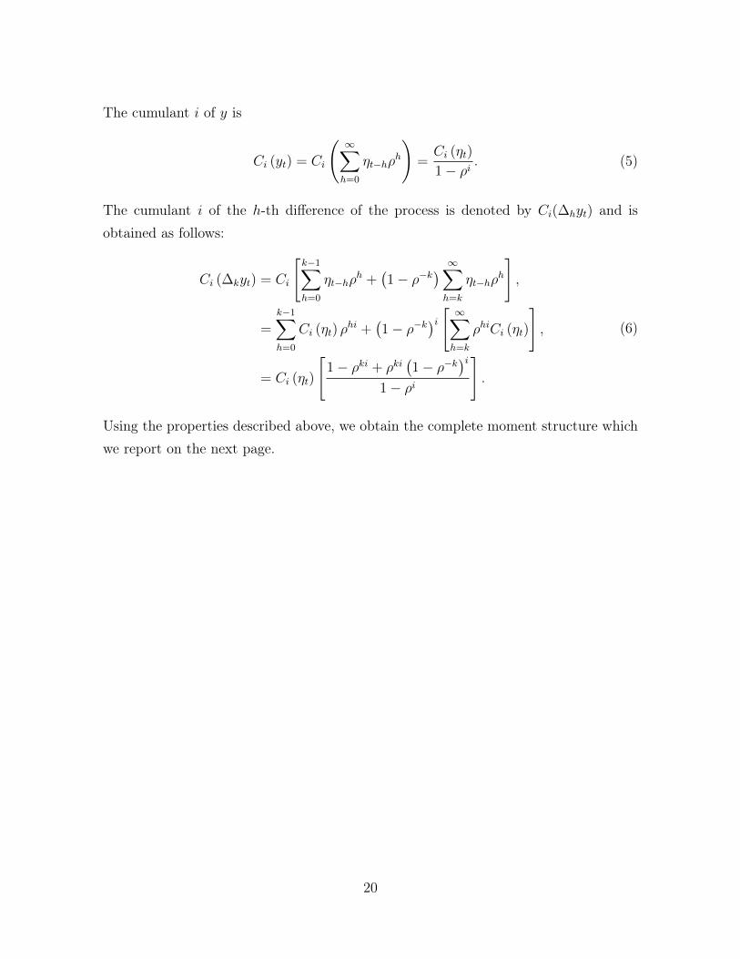
The cumulant i of y is

Ci (yt) = Ci

(∞∑h=0

ηt−hρh

)=Ci (ηt)

1− ρi. (5)

The cumulant i of the h-th difference of the process is denoted by Ci(∆hyt) and isobtained as follows:

Ci (∆kyt) = Ci

[k−1∑h=0

ηt−hρh +

(1− ρ−k

) ∞∑h=k

ηt−hρh

],

=k−1∑h=0

Ci (ηt) ρhi +

(1− ρ−k

)i [ ∞∑h=k

ρhiCi (ηt)

],

= Ci (ηt)

[1− ρki + ρki

(1− ρ−k

)i1− ρi

].

(6)

Using the properties described above, we obtain the complete moment structure whichwe report on the next page.

20

E(ηt) = p1µ1 + p2µ2,

E(η2t ) = p1(µ2

1 + σ21) + p2(µ2

2 + σ22),

E(η3t ) = p1(µ3

1 + 3µ1σ21) + p2(µ3

2 + 3µ2σ22),

E(η4t ) = p1(µ4

1 + 6µ21σ

21 + 3σ4

1) + p2(µ42 + 6µ2

2σ22 + 3σ4

2),

(7)

Var(ηt) = E(η2t )− E(ηt)

2,

S(ηt) =E(η3

t )− 3E(ηt)Var(ηt)− E(ηt)3

Std(ηt)3,

K(ηt) =E(η4

t )− 3E(ηt)4 + 6E(η2

t )E(ηt)2 − 4E(ηt)E(η3

t )

Var(ηt)2

(8)

E(yt) =E(ηt)

1− ρ,

Var (yt) =Var (ηt)

1− ρ2,

S (yt) = S(ηt)(1− ρ2)3/2

1− ρ3,

K (yt) = 3 +(1− ρ2)2(K(ηt)− 3)

1− ρ4,

(9)

E(∆kyt) = 0,

Var (∆kyt) =2Var (ηt)

[ρk − 1

]ρ2 − 1

,

S (∆kyt) =3S(ηt)ρ

k(ρk − 1

)2√

2 (ρ3 − 1)(ρk−1ρ2−1

)3/2,

K (∆kyt) =

(ρ2 − 1

)2{ (K(ηt)−3)(ρk−1)[(2ρk−1)ρk+1]ρ4−1

+6[ρk−1]

2

(ρ2−1)2

}2 [ρk − 1]

2 ,

(10)

Var(∆kyt) = Var(∆y)

(ρk − 1

)(ρ− 1)

,

S(∆kyt) = S(∆y)

√ρ2 − 1ρk−1√

(ρ+ 1)(ρk − 1),

K(∆kyt) = K(∆y)

(ρ2 + 1

) (ρ2 − 1

)2 (ρk − 1

)(2ρ3 + ρ2 + 1) (ρ4 − 1) [ρk − 1]

2 ×[(

2ρk − 1)ρk + 1

]+

(ρ2 − 1

)2 (ρk − 1

) ((2ρk − 1

)ρk + 1

)2 (ρ4 − 1) (ρk − 1)

2 ×

{−

3(−2ρ3 + ρ2 + 1

)2ρ3 + ρ2 + 1

+6(ρ4 − 1

) (ρk − 1

)2(ρ2 − 1)2 (ρk − 1) ((2ρk − 1) ρk + 1)

− 3

}.

(11)

21

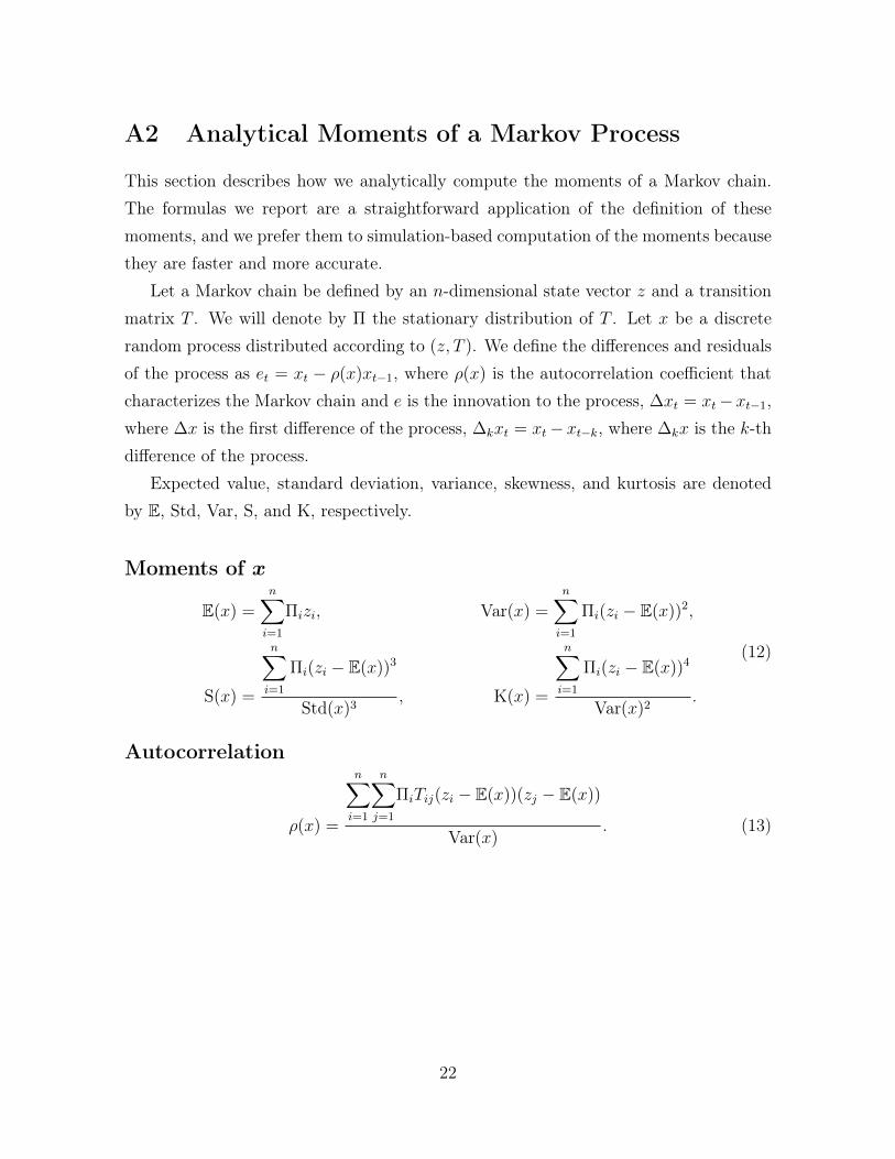
A2 Analytical Moments of a Markov Process

This section describes how we analytically compute the moments of a Markov chain.The formulas we report are a straightforward application of the definition of thesemoments, and we prefer them to simulation-based computation of the moments becausethey are faster and more accurate.

Let a Markov chain be defined by an n-dimensional state vector z and a transitionmatrix T . We will denote by Π the stationary distribution of T . Let x be a discreterandom process distributed according to (z, T ). We define the differences and residualsof the process as et = xt − ρ(x)xt−1, where ρ(x) is the autocorrelation coefficient thatcharacterizes the Markov chain and e is the innovation to the process, ∆xt = xt−xt−1,where ∆x is the first difference of the process, ∆kxt = xt− xt−k, where ∆kx is the k-thdifference of the process.

Expected value, standard deviation, variance, skewness, and kurtosis are denotedby E, Std, Var, S, and K, respectively.

Moments of x

E(x) =n∑i=1

Πizi, Var(x) =n∑i=1

Πi(zi − E(x))2,

S(x) =

n∑i=1

Πi(zi − E(x))3

Std(x)3, K(x) =

n∑i=1

Πi(zi − E(x))4

Var(x)2.

(12)

Autocorrelation

ρ(x) =

n∑i=1

n∑j=1

ΠiTij(zi − E(x))(zj − E(x))

Var(x). (13)

22

Moments of e

Let E be an n× n matrix, where each element is defined as follows: Ei,j = zj − ρ(x)zi.

Then the moments of e are given by

E(e) =n∑i=1

n∑j=1

ΠiTijEij, Var(e) =n∑i=1

n∑j=1

ΠiTij(Eij − E(e))2,

S(e) =

n∑i=1

ΠiTij(Eij − E(e))3

Std(e)3, K(e) =

n∑i=1

n∑j=1

ΠiTij(Eij − E(e))4

Var(e)2.

(14)

Moments of ∆x

Let δ be a n × n matrix, where each element is defined as follows: δi,j = zj − zi Thenthe moments of ∆x are given by:

E(∆x) =n∑i=1

n∑j=1

ΠiTijδij, Var(∆x) =n∑i=1

n∑j=1

ΠiTij(δij − E(∆x))2,

S(∆x) =

n∑i=1

ΠiTij(δij − E(∆x))3

Std(∆x)3, K(∆x) =

n∑i=1

n∑j=1

ΠiTij(δij − E(∆x))4

Var(∆x)2.

(15)

Moments of ∆kx

To calculate the moments of ∆kx, it is sufficient to replace Tij with (T k)ij in the formulasfor ∆x. Notice that (T k)ij is the element on row i, column j, of a matrix obtained bymultiplying T by itself k times.

A3 Speed and performance

In order to assess the practical implementability of the ET method we run a globaloptimization algorithm as outlined by Guvenen (2017) with 400 restarts. The set upof the problem is identical to that of Section 4.1. In Table 5 we report, in seconds, thetime necessary to perform the optimization procedure. Furthermore we report usingthe same format as in Table 4 the average percentage deviation of the moments fromtheir targets.

23

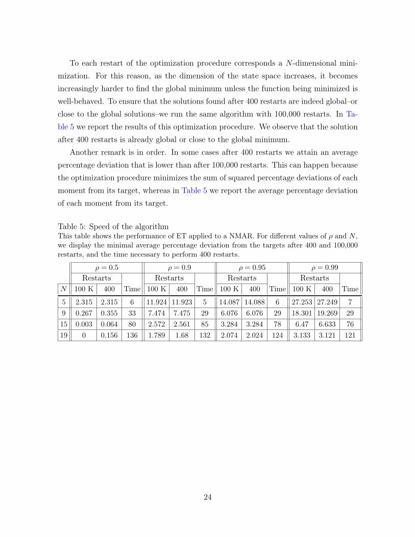
To each restart of the optimization procedure corresponds a N -dimensional mini-mization. For this reason, as the dimension of the state space increases, it becomesincreasingly harder to find the global minimum unless the function being minimized iswell-behaved. To ensure that the solutions found after 400 restarts are indeed global–orclose to the global solutions–we run the same algorithm with 100,000 restarts. In Ta-ble 5 we report the results of this optimization procedure. We observe that the solutionafter 400 restarts is already global or close to the global minimum.

Another remark is in order. In some cases after 400 restarts we attain an averagepercentage deviation that is lower than after 100,000 restarts. This can happen becausethe optimization procedure minimizes the sum of squared percentage deviations of eachmoment from its target, whereas in Table 5 we report the average percentage deviationof each moment from its target.

Table 5: Speed of the algorithmThis table shows the performance of ET applied to a NMAR. For different values of ρ and N ,we display the minimal average percentage deviation from the targets after 400 and 100,000restarts, and the time necessary to perform 400 restarts.

ρ = 0.5 ρ = 0.9 ρ = 0.95 ρ = 0.99

Restarts Restarts Restarts RestartsN 100 K 400 Time 100 K 400 Time 100 K 400 Time 100 K 400 Time

5 2.315 2.315 6 11.924 11.923 5 14.087 14.088 6 27.253 27.249 79 0.267 0.355 33 7.474 7.475 29 6.076 6.076 29 18.301 19.269 2915 0.003 0.064 80 2.572 2.561 85 3.284 3.284 78 6.47 6.633 7619 0 0.156 136 1.789 1.68 132 2.074 2.024 124 3.133 3.121 121

24

A4 Figures

Figure 7: Feasible combinations of {S(η),K(η)} with a mixture of 2 or 3 normalsIn this figure, we show what combinations of kurtosis, K(η), and skewness, S(η), are feasiblewhen calibrating a mixture of two or three normals. The combinations NE of each line areexactly attainable. This figure shows that using a mixture of three normals expands the setof feasible combinations only moderately.

� ��

� �� -�

-�

-�

-�

-�

�(η)

�(η)

25

ONLINE APPENDIXNOT FOR PUBLICATION

In this appendix we discuss some issues that are not central to our paper but arenonetheless relevant. In Appendix B1 we document how several methods for discretizinga Gaussian AR(1) calibrate a discrete process that features substancial kurtosis whenthe process is persistent. In light of this fact in Section B1.1 we show how the ETmethod can be used to calibrate a discrete process that matches kurtosis more precisely.In doing so ET trades-off the accuracy of higher order moments with the accuracy ofvariance and autocorrelation.

In Appendix B2 we study the limitations of NMAR in reproducing persistent skew-ness and kurtosis. To improve on the limitations of NMAR we generalize it by aug-menting it with a temporary Gaussian shock. Section B2.1 studies this new process,which we call NMART. We find that NMART is flexible enough to feature persistentskewness and kurtosis. Finally, in Appendix B3 we discretize an NMART using themethod of simulated moments and we provide an illustration.

B1 Kurtosis of the Innovations

In this section, we discuss a calibration error that is common to most familiar methodsused for discretizing an AR(1) process with a Gaussian innovation. Let y denote acontinuous process, with an AR(1) representation,

yt = ρyt−1 + εt, (16)

where |ρ| < 1 and εt ∼ N (0, σ2). We denote the Markov chain by (z, T ), with xt ∼(z, T ) and et = xt− ρ̂xt−1, where ρ̂ is the first-order autocorrelation associated with xt.

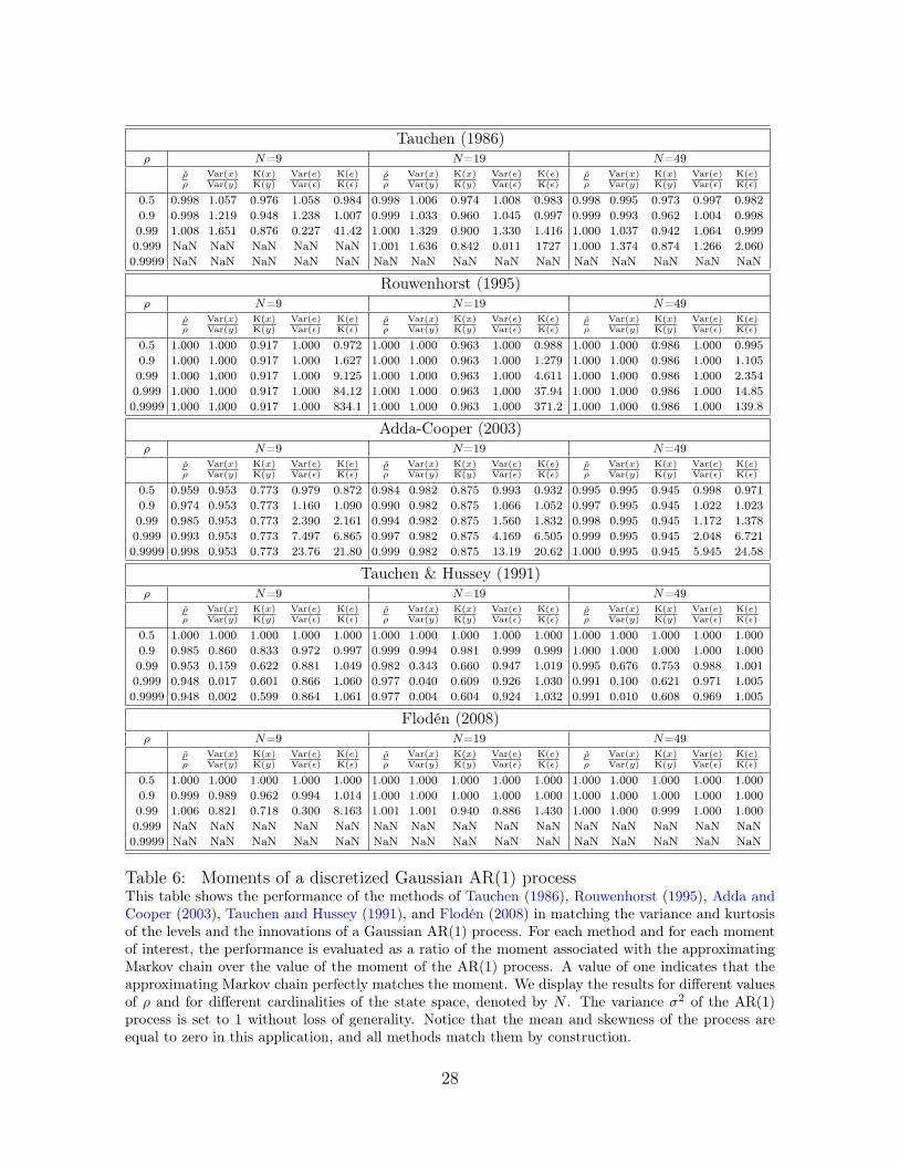
To report the results we use the same format as in Table 4. In particular, Table 6shows that for a highly persistent AR(1) process, standard discretization methods fea-ture a very high kurtosis in the innovation. For example, if we consider a 9-state Markovchain with an autocorrelation of 0.99 and use Rouwenhorst’s method, the kurtosis ofthe innovation implied by the discretization method is about 27, eight times higher thanthe kurtosis of the Gaussian innovation, which equals 3. The method of Tauchen andHussey (1991) performs much better with respect to the kurtosis of the innovations,

26

but it misses the variance of the levels entirely. A notable exception is the methodof Flodén (2008), which is more accurate and reasonably matches the moments of theinnovations and the levels, though it becomes less precise as ρ approaches 1.

A Markov Chain typically features non-zero skewness and excess kurtosis even if itdiscretizes a Gaussian AR(1). This feature is mentioned in Gospodinov and Lkhagva-suren (2014), but to the best of our knowledge it has never been documented in detail.In fact, even if the methods we discuss in Table 6 are not meant to match the kurtosisof the process, it is important to understand the extent of this calibration error.

B1.1 Using ET to discretize a Gaussian AR(1)

In this section we show that ET can be applied to discretize a Gaussian AR(1). Evenif this is not the principal application of the ET method, it is interesting to show howET can be applied to trade-off the precision of the first two moments with the precisionof skewness and kurtosis.

As explained in Section 4, the ET method differs from Tauchen (1986) in two ways:(i) the innovations are distributed as a normal mixture, and (ii) the states are placedoptimally with respect to a set of targeted moments. Because this application differsfrom Tauchen (1986) only in the second direction, it establishes a connection withthe existing literature and allows a comparison of the ET method with other existingmethods. Furthermore, in light of the findings we report in Table 6, this applicationshows how it is possible to trade-off between accurately matching the first two andhigher order moments.

Since the innovations are symmetrically distributed around 0, in this applicationwe impose that z is symmetric around 0. Then E (x) = E (e) = S (x) = S (e) = 0

by construction and therefore we only target ρ,Var (y) ,Var (ε) ,K (y) ,K (ε). In thisapplication Var (ε) = 1, K (y) = K (ε) = 3 whereas the value of Var (y) changes with ρ.In Table 7 we report the performance of our calibration in the usual format.

We conclude this section comparing the methods graphically. We consider a Gaus-sian AR(1) process with ρ = 0.99 and unit variance. We then apply the differentmethods discussed so far and in Figure 8, Figure 9 and Figure 10 we display the his-togram of the stationary distribution of the levels and innovations.

In Figure 9, it is interesting to observe how the methods of Tauchen and Rouwen-

27

Tauchen (1986)ρ N=9 N=19 N=49

ρ̂ρ

Var(x)Var(y)

K(x)K(y)

Var(e)Var(ε)

K(e)K(ε)

ρ̂ρ

Var(x)Var(y)

K(x)K(y)

Var(e)Var(ε)

K(e)K(ε)

ρ̂ρ

Var(x)Var(y)

K(x)K(y)

Var(e)Var(ε)

K(e)K(ε)

0.5 0.998 1.057 0.976 1.058 0.984 0.998 1.006 0.974 1.008 0.983 0.998 0.995 0.973 0.997 0.9820.9 0.998 1.219 0.948 1.238 1.007 0.999 1.033 0.960 1.045 0.997 0.999 0.993 0.962 1.004 0.9980.99 1.008 1.651 0.876 0.227 41.42 1.000 1.329 0.900 1.330 1.416 1.000 1.037 0.942 1.064 0.9990.999 NaN NaN NaN NaN NaN 1.001 1.636 0.842 0.011 1727 1.000 1.374 0.874 1.266 2.0600.9999 NaN NaN NaN NaN NaN NaN NaN NaN NaN NaN NaN NaN NaN NaN NaN

Rouwenhorst (1995)ρ N=9 N=19 N=49

ρ̂ρ

Var(x)Var(y)

K(x)K(y)

Var(e)Var(ε)

K(e)K(ε)

ρ̂ρ

Var(x)Var(y)

K(x)K(y)

Var(e)Var(ε)

K(e)K(ε)

ρ̂ρ

Var(x)Var(y)

K(x)K(y)

Var(e)Var(ε)

K(e)K(ε)

0.5 1.000 1.000 0.917 1.000 0.972 1.000 1.000 0.963 1.000 0.988 1.000 1.000 0.986 1.000 0.9950.9 1.000 1.000 0.917 1.000 1.627 1.000 1.000 0.963 1.000 1.279 1.000 1.000 0.986 1.000 1.1050.99 1.000 1.000 0.917 1.000 9.125 1.000 1.000 0.963 1.000 4.611 1.000 1.000 0.986 1.000 2.3540.999 1.000 1.000 0.917 1.000 84.12 1.000 1.000 0.963 1.000 37.94 1.000 1.000 0.986 1.000 14.850.9999 1.000 1.000 0.917 1.000 834.1 1.000 1.000 0.963 1.000 371.2 1.000 1.000 0.986 1.000 139.8

Adda-Cooper (2003)ρ N=9 N=19 N=49

ρ̂ρ

Var(x)Var(y)

K(x)K(y)

Var(e)Var(ε)

K(e)K(ε)

ρ̂ρ

Var(x)Var(y)

K(x)K(y)

Var(e)Var(ε)

K(e)K(ε)

ρ̂ρ

Var(x)Var(y)

K(x)K(y)

Var(e)Var(ε)

K(e)K(ε)

0.5 0.959 0.953 0.773 0.979 0.872 0.984 0.982 0.875 0.993 0.932 0.995 0.995 0.945 0.998 0.9710.9 0.974 0.953 0.773 1.160 1.090 0.990 0.982 0.875 1.066 1.052 0.997 0.995 0.945 1.022 1.0230.99 0.985 0.953 0.773 2.390 2.161 0.994 0.982 0.875 1.560 1.832 0.998 0.995 0.945 1.172 1.3780.999 0.993 0.953 0.773 7.497 6.865 0.997 0.982 0.875 4.169 6.505 0.999 0.995 0.945 2.048 6.7210.9999 0.998 0.953 0.773 23.76 21.80 0.999 0.982 0.875 13.19 20.62 1.000 0.995 0.945 5.945 24.58

Tauchen & Hussey (1991)ρ N=9 N=19 N=49

ρ̂ρ

Var(x)Var(y)

K(x)K(y)

Var(e)Var(ε)

K(e)K(ε)

ρ̂ρ

Var(x)Var(y)

K(x)K(y)

Var(e)Var(ε)

K(e)K(ε)

ρ̂ρ

Var(x)Var(y)

K(x)K(y)

Var(e)Var(ε)

K(e)K(ε)

0.5 1.000 1.000 1.000 1.000 1.000 1.000 1.000 1.000 1.000 1.000 1.000 1.000 1.000 1.000 1.0000.9 0.985 0.860 0.833 0.972 0.997 0.999 0.994 0.981 0.999 0.999 1.000 1.000 1.000 1.000 1.0000.99 0.953 0.159 0.622 0.881 1.049 0.982 0.343 0.660 0.947 1.019 0.995 0.676 0.753 0.988 1.0010.999 0.948 0.017 0.601 0.866 1.060 0.977 0.040 0.609 0.926 1.030 0.991 0.100 0.621 0.971 1.0050.9999 0.948 0.002 0.599 0.864 1.061 0.977 0.004 0.604 0.924 1.032 0.991 0.010 0.608 0.969 1.005

Flodén (2008)ρ N=9 N=19 N=49

ρ̂ρ

Var(x)Var(y)

K(x)K(y)

Var(e)Var(ε)

K(e)K(ε)

ρ̂ρ

Var(x)Var(y)

K(x)K(y)

Var(e)Var(ε)

K(e)K(ε)

ρ̂ρ

Var(x)Var(y)

K(x)K(y)

Var(e)Var(ε)

K(e)K(ε)

0.5 1.000 1.000 1.000 1.000 1.000 1.000 1.000 1.000 1.000 1.000 1.000 1.000 1.000 1.000 1.0000.9 0.999 0.989 0.962 0.994 1.014 1.000 1.000 1.000 1.000 1.000 1.000 1.000 1.000 1.000 1.0000.99 1.006 0.821 0.718 0.300 8.163 1.001 1.001 0.940 0.886 1.430 1.000 1.000 0.999 1.000 1.0000.999 NaN NaN NaN NaN NaN NaN NaN NaN NaN NaN NaN NaN NaN NaN NaN0.9999 NaN NaN NaN NaN NaN NaN NaN NaN NaN NaN NaN NaN NaN NaN NaN

Table 6: Moments of a discretized Gaussian AR(1) processThis table shows the performance of the methods of Tauchen (1986), Rouwenhorst (1995), Adda andCooper (2003), Tauchen and Hussey (1991), and Flodén (2008) in matching the variance and kurtosisof the levels and the innovations of a Gaussian AR(1) process. For each method and for each momentof interest, the performance is evaluated as a ratio of the moment associated with the approximatingMarkov chain over the value of the moment of the AR(1) process. A value of one indicates that theapproximating Markov chain perfectly matches the moment. We display the results for different valuesof ρ and for different cardinalities of the state space, denoted by N . The variance σ2 of the AR(1)process is set to 1 without loss of generality. Notice that the mean and skewness of the process areequal to zero in this application, and all methods match them by construction.

28

horst cluster the states around 0 and place only little mass at more than 4 standarddeviation from 0. This is a graphical illustration of the excessive kurtosis that thesemethods generate.

29

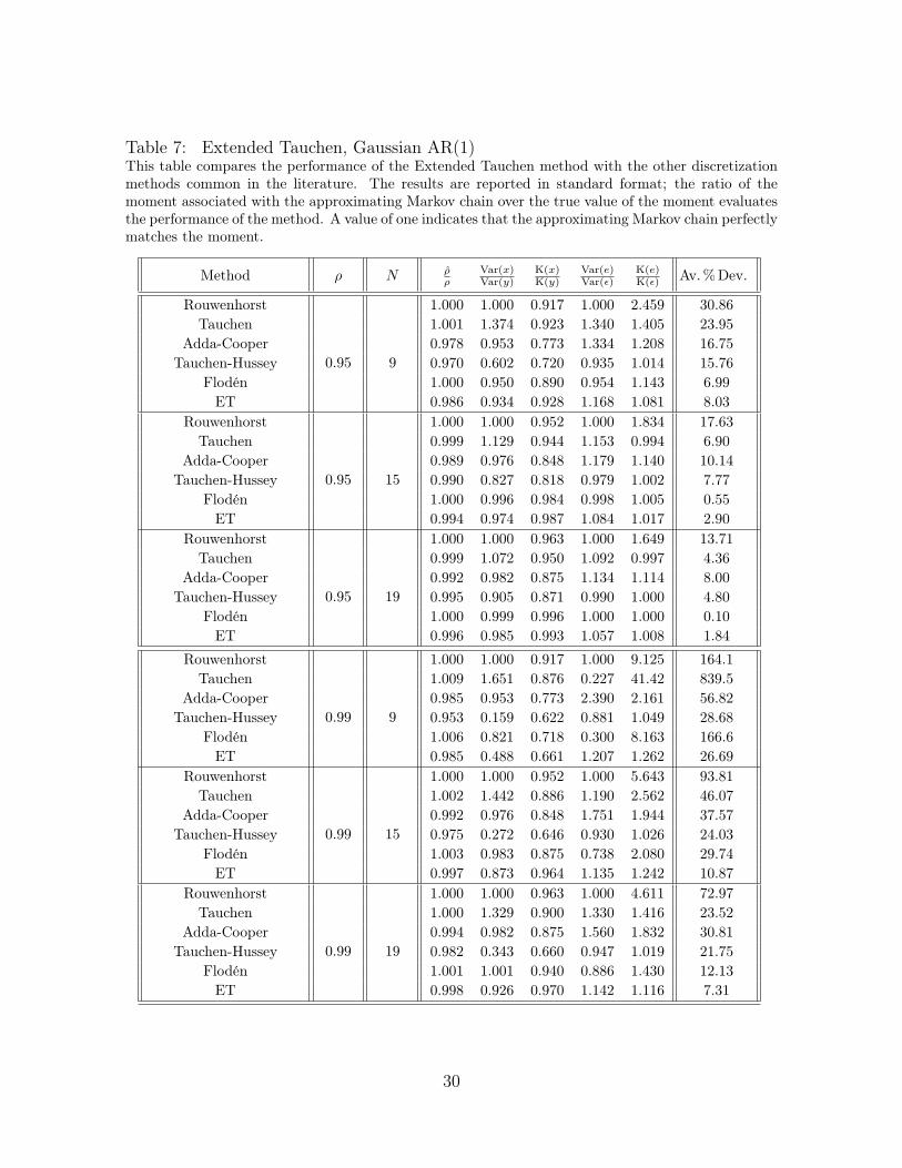
Table 7: Extended Tauchen, Gaussian AR(1)This table compares the performance of the Extended Tauchen method with the other discretizationmethods common in the literature. The results are reported in standard format; the ratio of themoment associated with the approximating Markov chain over the true value of the moment evaluatesthe performance of the method. A value of one indicates that the approximating Markov chain perfectlymatches the moment.

Method ρ N ρ̂ρ

Var(x)Var(y)

K(x)K(y)

Var(e)Var(ε)

K(e)K(ε) Av.%Dev.

Rouwenhorst

0.95 9

1.000 1.000 0.917 1.000 2.459 30.86Tauchen 1.001 1.374 0.923 1.340 1.405 23.95

Adda-Cooper 0.978 0.953 0.773 1.334 1.208 16.75Tauchen-Hussey 0.970 0.602 0.720 0.935 1.014 15.76

Flodén 1.000 0.950 0.890 0.954 1.143 6.99ET 0.986 0.934 0.928 1.168 1.081 8.03

Rouwenhorst

0.95 15

1.000 1.000 0.952 1.000 1.834 17.63Tauchen 0.999 1.129 0.944 1.153 0.994 6.90


Flodén 1.000 0.996 0.984 0.998 1.005 0.55ET 0.994 0.974 0.987 1.084 1.017 2.90

Rouwenhorst

0.95 19

1.000 1.000 0.963 1.000 1.649 13.71Tauchen 0.999 1.072 0.950 1.092 0.997 4.36


Flodén 1.000 0.999 0.996 1.000 1.000 0.10ET 0.996 0.985 0.993 1.057 1.008 1.84

Rouwenhorst

0.99 9

1.000 1.000 0.917 1.000 9.125 164.1Tauchen 1.009 1.651 0.876 0.227 41.42 839.5


Flodén 1.006 0.821 0.718 0.300 8.163 166.6ET 0.985 0.488 0.661 1.207 1.262 26.69

Rouwenhorst

0.99 15

1.000 1.000 0.952 1.000 5.643 93.81Tauchen 1.002 1.442 0.886 1.190 2.562 46.07


Flodén 1.003 0.983 0.875 0.738 2.080 29.74ET 0.997 0.873 0.964 1.135 1.242 10.87

Rouwenhorst

0.99 19

1.000 1.000 0.963 1.000 4.611 72.97Tauchen 1.000 1.329 0.900 1.330 1.416 23.52


Flodén 1.001 1.001 0.940 0.886 1.430 12.13ET 0.998 0.926 0.970 1.142 1.116 7.31

30

Figure 8: Histograms of the Levels, Gaussian AR(1): ρ = 0.99, N=9This figure displays the histogram of the levels (x) implied by the Markov chain of the methods ofTauchen (1986), Rouwenhorst (1995), Adda and Cooper (2003), Tauchen and Hussey (1991), andFlodén (2008). In this example, ρ = 0.99, the variance of the shocks equals 1 and we use 9 states. Thex-axis shows the state space and the y-axis the stationary probability of each state.

-15 0 15

0.1

0.2

Tauchen (1986)

-15 0 15

0.1

0.2

Rouwenhorst (1995)

-15 0 15

0.05

0.1

Tauchen-Hussey (1991)

-15 0 15

0.05

0.1

Adda-Cooper (2003)

-15 0 15

0.05

0.1

Flodén (2008)

-15 0 15

0.05

0.1

ET

31

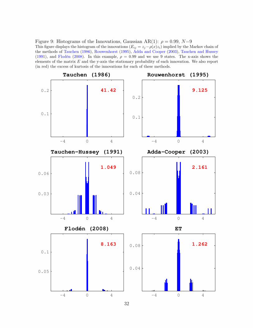
Figure 9: Histograms of the Innovations, Gaussian AR(1): ρ = 0.99, N=9This figure displays the histogram of the innovations (Eij = zj−ρ(x)zi) implied by the Markov chain ofthe methods of Tauchen (1986), Rouwenhorst (1995), Adda and Cooper (2003), Tauchen and Hussey(1991), and Flodén (2008). In this example, ρ = 0.99 and we use 9 states. The x-axis shows theelements of the matrix E and the y-axis the stationary probability of each innovation. We also report(in red) the excess of kurtosis of the innovations for each of these methods.

-4 0 4

0.1

0.2 41.42

Tauchen (1986)

-4 0 4

0.1

0.2

9.125

Rouwenhorst (1995)

-4 0 4

0.03

0.06 1.049


-4 0 4

0.04

0.08 2.161

Adda-Cooper (2003)

-4 0 4

0.05

0.1

8.163

Flodén (2008)

-4 0 4

0.04

0.08 1.262

ET

32

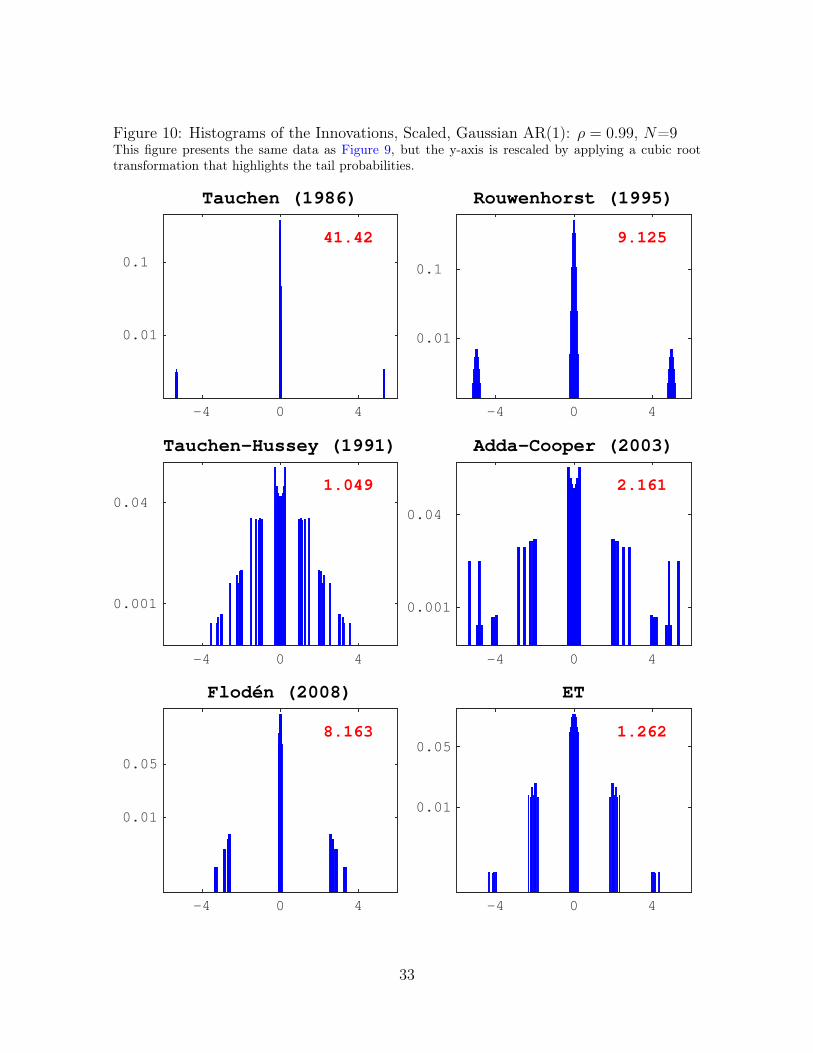
Figure 10: Histograms of the Innovations, Scaled, Gaussian AR(1): ρ = 0.99, N=9This figure presents the same data as Figure 9, but the y-axis is rescaled by applying a cubic roottransformation that highlights the tail probabilities.

-4 0 4

0.01

0.1

41.42

Tauchen (1986)

-4 0 4

0.01

0.1

9.125

Rouwenhorst (1995)

-4 0 4

0.001

0.04 1.049


-4 0 4

0.001

0.04

2.161

Adda-Cooper (2003)

-4 0 4

0.01

0.05

8.163

Flodén (2008)

-4 0 4

0.01

0.05 1.262

ET

33

B2 Limitations of NMAR and NMART

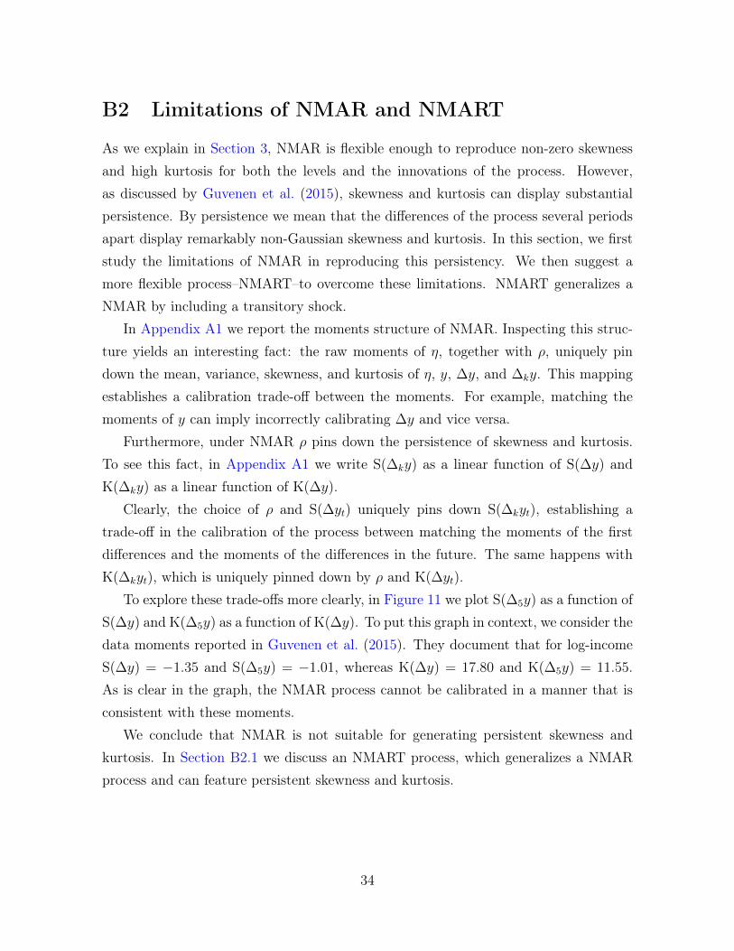
As we explain in Section 3, NMAR is flexible enough to reproduce non-zero skewnessand high kurtosis for both the levels and the innovations of the process. However,as discussed by Guvenen et al. (2015), skewness and kurtosis can display substantialpersistence. By persistence we mean that the differences of the process several periodsapart display remarkably non-Gaussian skewness and kurtosis. In this section, we firststudy the limitations of NMAR in reproducing this persistency. We then suggest amore flexible process–NMART–to overcome these limitations. NMART generalizes aNMAR by including a transitory shock.

In Appendix A1 we report the moments structure of NMAR. Inspecting this struc-ture yields an interesting fact: the raw moments of η, together with ρ, uniquely pindown the mean, variance, skewness, and kurtosis of η, y, ∆y, and ∆ky. This mappingestablishes a calibration trade-off between the moments. For example, matching themoments of y can imply incorrectly calibrating ∆y and vice versa.

Furthermore, under NMAR ρ pins down the persistence of skewness and kurtosis.To see this fact, in Appendix A1 we write S(∆ky) as a linear function of S(∆y) andK(∆ky) as a linear function of K(∆y).

Clearly, the choice of ρ and S(∆yt) uniquely pins down S(∆kyt), establishing atrade-off in the calibration of the process between matching the moments of the firstdifferences and the moments of the differences in the future. The same happens withK(∆kyt), which is uniquely pinned down by ρ and K(∆yt).

To explore these trade-offs more clearly, in Figure 11 we plot S(∆5y) as a function ofS(∆y) and K(∆5y) as a function of K(∆y). To put this graph in context, we consider thedata moments reported in Guvenen et al. (2015). They document that for log-incomeS(∆y) = −1.35 and S(∆5y) = −1.01, whereas K(∆y) = 17.80 and K(∆5y) = 11.55.As is clear in the graph, the NMAR process cannot be calibrated in a manner that isconsistent with these moments.

We conclude that NMAR is not suitable for generating persistent skewness andkurtosis. In Section B2.1 we discuss an NMART process, which generalizes a NMARprocess and can feature persistent skewness and kurtosis.

34

Figure 11: S(∆5y) and K(∆5y)This figure shows S(∆5y) and K(∆5y) as a function of ρ, given that S(∆y) = −1.35 andK(∆y) = 17.8.

� ��

-��

-��

-��

-��

-��

-��

��

�(Δ��)

�(Δ�)=-��

ρ� ��

�

�

��

��

��

��

��

�(Δ��)

�(Δ�)=��

ρ

B2.1 NMART Process

In this section, we introduce the NMART process, an autoregressive process with normalmixture shocks and a transitory shock. In fact, NMART is an NMAR process plus atransitory Gaussian shock. As we discuss in this section, including the transitory shockis crucial to modeling persistent skewness and kurtosis.

The NMART process has the following representation:

yt = zt + εt (17)

zt = ρzt−1 + ηt,

where

ηt ∼

{N(µ1, σ


N(µ2, σ22) with probability p2,

εt ∼ N(0, σ2ε ).

To simplify the exposition, we write the variance of the transitory shock as a constant αof the variance of the permanent shock, that is, Var (εt) = αVar (ηt). Clearly, if α = 0,then yt is NMAR.

To appreciate why the transitory component of the process plays a central role inmodeling persistent skewness and kurtosis we obtain analytical formulas of variance,skewness, and kurtosis of ∆ky.

35

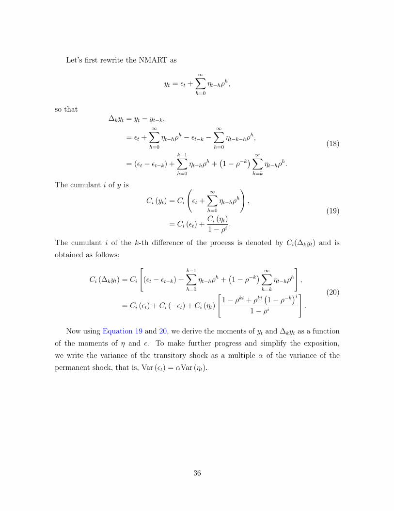
Let’s first rewrite the NMART as

yt = εt +∞∑h=0

ηt−hρh,

so that∆kyt = yt − yt−k,

= εt +∞∑h=0

ηt−hρh − εt−k −

∞∑h=0

ηt−k−hρh,

= (εt − εt−k) +k−1∑h=0

ηt−hρh +

(1− ρ−k

) ∞∑h=k

ηt−hρh.

(18)

The cumulant i of y is

Ci (yt) = Ci

(εt +

∞∑h=0

ηt−hρh

),

= Ci (εt) +Ci (ηt)

1− ρi.

(19)

The cumulant i of the k-th difference of the process is denoted by Ci(∆kyt) and isobtained as follows:

Ci (∆kyt) = Ci

[(εt − εt−k) +

k−1∑h=0

ηt−hρh +

(1− ρ−k

) ∞∑h=k

ηt−hρh

],

= Ci (εt) + Ci (−εt) + Ci (ηt)

[1− ρki + ρki

(1− ρ−k

)i1− ρi

].

(20)

Now using Equation 19 and 20, we derive the moments of yt and ∆kyt as a functionof the moments of η and ε. To make further progress and simplify the exposition,we write the variance of the transitory shock as a multiple α of the variance of thepermanent shock, that is, Var (εt) = αVar (ηt).

36

Var (yt) = Var (ηt)

(α +

1

1− ρ2

),

S (yt) =S (ηt)

(1− ρ3)(α + 1

1−ρ2

)3/2,

K (yt) =3(α + 1

1−ρ2

)2

+ 3−K(ηt)ρ4−1(

α + 11−ρ2

)2 ,

(21)

Var (∆kyt) =2Var (ηt)

[α (ρ2 − 1) + ρk − 1

]ρ2 − 1

,

S (∆kyt) =3S(ηt)ρ

k(ρk − 1

)2√

2 (ρ3 − 1)(α(ρ2−1)+ρk−1

ρ2−1

)3/2,

K (∆kyt) =

(ρ2 − 1)2

{(K(ηt)−3)(ρk−1)[(2ρk−1)ρk+1]

ρ4−1+

6[α(ρ2−1)+ρk−1]2

(ρ2−1)2

}2 [α (ρ2 − 1) + ρk − 1]2

,

(22)

Var(∆kyt) = Var(∆yt)(αρ2 − α + ρk − 1

)(ρ− 1)(αρ+ α + 1)

,

S(∆kyt) = S(∆yt)(ρ+ 1)

√αρ+α+1ρ+1

(α + 1

ρ+1

)ρk−1

(ρk − 1

)(αρ2 − α + ρk − 1)

√αρ2−α+ρk−1

ρ2−1

,

K(∆kyt) = K(∆yt)(ρ2 + 1) (ρ2 − 1)

2(αρ+ α + 1)2

(ρk − 1

)(2ρ3 + ρ2 + 1) (ρ4 − 1) [α (ρ2 − 1) + ρk − 1]2

×[(

2ρk − 1)ρk + 1

]+

(ρ2 − 1)2 (ρk − 1

) ((2ρk − 1

)ρk + 1

)2 (ρ4 − 1) (α (ρ2 − 1) + ρk − 1)2

×

{− 3 [2α2(ρ+ 1)2 (ρ2 + 1) + 4α (ρ3 + ρ2 + ρ+ 1)]

2ρ3 + ρ2 + 1

− 3 (−2ρ3 + ρ2 + 1)

2ρ3 + ρ2 + 1

+6 (ρ4 − 1)

(α (ρ2 − 1) + ρk − 1

)2

(ρ2 − 1)2 (ρk − 1) ((2ρk − 1) ρk + 1)− 3

}.

(23)

37

Based on these formulas, our main findings can be summarized as follows:

(a) Var (∆ky) is a linear function of Var(η). For a given value of Var(η), Var (∆ky) isincreasing in α.

To study the persistence of variance, one can rewrite Var (∆ky) as a function ofVar (∆y): the relationship is linear, and it is a function of α, ρ, and t. As expected,for a given value of Var (∆y), Var (∆ky) is decreasing in α. In fact, as α increases,the magnitude of the temporary shock increases relative to the permanent shock.

(b) For the case S(η) < 0, S (∆ky) is linear in S(η), and it also depends on α, ρ, and t:S (∆ky) is increasing in α for a given S(η).6

To study the persistence of skewness, one can rewrite S (∆ky) as a linear functionof S (∆y), which also depends on α, ρ, and t. For a given value of S (∆y), S (∆ky) isdecreasing in α. This last fact is particularly important because it allows the processto capture the persistence in skewness; increasing α increases S (∆ky) /S (∆y).

(c) K (∆ky) is linear in K(η), and it varies with α, ρ, and t. K (∆ky) is decreasing inα for a given K(η).

To study the persistence of kurtosis, one can rewrite K (∆ky) as a linear functionof K (∆y), which also depends on α, ρ, and t. For a given value of K (∆y), K (∆ky)

is increasing in α. This feature allows the process to capture the persistence inkurtosis, as increasing α increases K (∆ky) /K (∆y).

In Figure 12 we plot how the persistence of variance, skewness, and kurtosis variesas a function of α. We repeat this exercise for selected values of ρ and assume thatVar(∆y), S(∆y), and K(∆y) take on the values in Guvenen et al. (2015). To illustratethe pattern of persistence, we plot the relationships reported in Equation 23, whichallow us to express Var(∆ky) as a function of Var(∆y), S(∆ky) as a function of S(∆y),and K(∆ky) as a function of K(∆y).

These findings show that varying α increases the persistence of skewness and kurto-sis. Now we explore what combinations of variance, skewness, and kurtosis are achiev-able. In fact, two issues affect what combinations of moments are attainable. (i) Sinceηt is a mixture of two normals, it may not admit a calibration featuring some combi-nations of {Var(η), S(η),K(η)}. (ii) Since the moments of ∆ky are a function of α, ρ,

6If S(η) > 0, then S (∆ky) is decreasing in α and S (∆ky) /S (∆y) is increasing in α.

38

Figure 12: Persistence of Variance, Skewness, and Kurtosis as a function of αIn this figure we fix Var(∆y) = 0.23, S(∆y) = −1.35, and K(∆y) = 17.8, as reported inGuvenen et al. (2015). We then plot Var(∆ky), S(∆ky), and K(∆ky) as a function of α, fork = 5, 10. Increasing α makes variance less persistent, whereas skewness and kurtosis becomemore persistent. When α = 0, the NMART process boils down to an NMAR process.

��(Δ��)

ρ=�� ρ=�� ρ=��

� ��

��

�

��

�

α

��(Δ��)

ρ=�� ρ=�� ρ=��

� ��

��

�

��

�

α

�(Δ��)

ρ=��ρ=��

ρ=��

� ��

�

-��

-�

-��

-�

α

�(Δ��)

ρ=��ρ=��

ρ=��

� ��

�

-��

-�

-��

-�

α

�(Δ��)

ρ=��

ρ=��

ρ=��

� ��

�

��

��

��

α

�(Δ��)

ρ=��

ρ=��

ρ=��

� ��

�

��

��

��

α

39

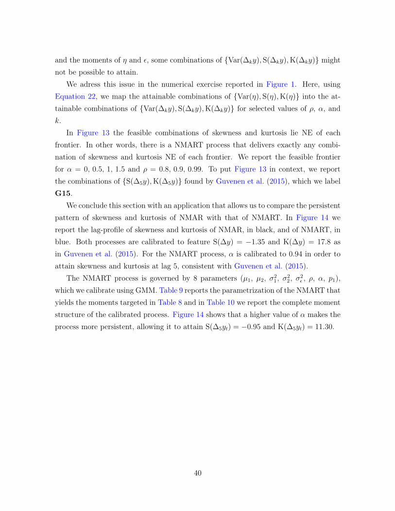
and the moments of η and ε, some combinations of {Var(∆ky), S(∆ky),K(∆ky)} mightnot be possible to attain.

We adress this issue in the numerical exercise reported in Figure 1. Here, usingEquation 22, we map the attainable combinations of {Var(η), S(η),K(η)} into the at-tainable combinations of {Var(∆ky), S(∆ky),K(∆ky)} for selected values of ρ, α, andk.

In Figure 13 the feasible combinations of skewness and kurtosis lie NE of eachfrontier. In other words, there is a NMART process that delivers exactly any combi-nation of skewness and kurtosis NE of each frontier. We report the feasible frontierfor α = 0, 0.5, 1, 1.5 and ρ = 0.8, 0.9, 0.99. To put Figure 13 in context, we reportthe combinations of {S(∆5y),K(∆5y)} found by Guvenen et al. (2015), which we labelG15.

We conclude this section with an application that allows us to compare the persistentpattern of skewness and kurtosis of NMAR with that of NMART. In Figure 14 wereport the lag-profile of skewness and kurtosis of NMAR, in black, and of NMART, inblue. Both processes are calibrated to feature S(∆y) = −1.35 and K(∆y) = 17.8 asin Guvenen et al. (2015). For the NMART process, α is calibrated to 0.94 in order toattain skewness and kurtosis at lag 5, consistent with Guvenen et al. (2015).

The NMART process is governed by 8 parameters (µ1, µ2, σ21, σ2

2, σ2ε , ρ, α, p1),

which we calibrate using GMM. Table 9 reports the parametrization of the NMART thatyields the moments targeted in Table 8 and in Table 10 we report the complete momentstructure of the calibrated process. Figure 14 shows that a higher value of α makes theprocess more persistent, allowing it to attain S(∆5yt) = −0.95 and K(∆5yt) = 11.30.

40

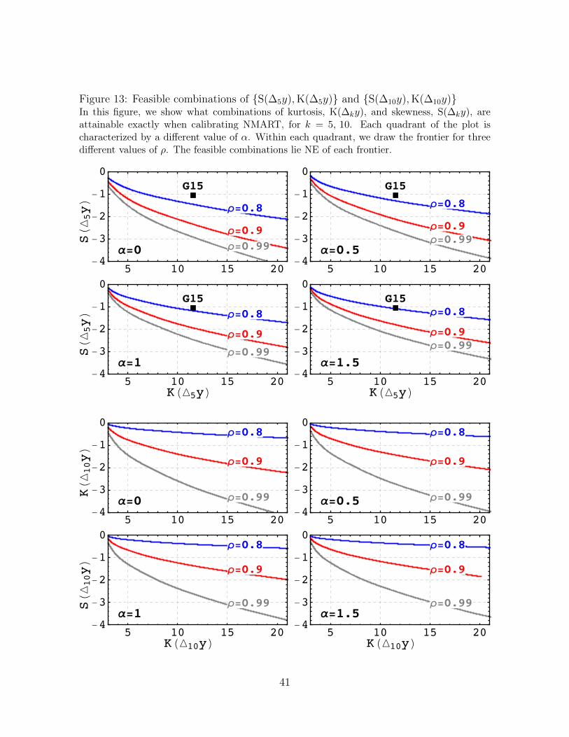
Figure 13: Feasible combinations of {S(∆5y),K(∆5y)} and {S(∆10y),K(∆10y)}In this figure, we show what combinations of kurtosis, K(∆ky), and skewness, S(∆ky), areattainable exactly when calibrating NMART, for k = 5, 10. Each quadrant of the plot ischaracterized by a different value of α. Within each quadrant, we draw the frontier for threedifferent values of ρ. The feasible combinations lie NE of each frontier.

�(Δ��)

α=�

ρ=��

ρ=��

ρ=��

��◼◼

� �� -�

-�

-�

-�

�

α=��

ρ=��

ρ=��ρ=��

��◼◼

� �� -�

-�

-�

-�

�

�(Δ��)

α=�

ρ=��

ρ=��

ρ=��

��◼◼

� �� -�

-�

-�

-�

�

�(Δ��)

α=��

ρ=��

ρ=��ρ=��

��◼◼

� �� -�

-�

-�

-�

�

�(Δ��)

�(Δ��)

α=�

ρ=��

ρ=��

ρ=��

� �� -�

-�

-�

-�

�

α=��

ρ=��

ρ=��

ρ=��

� �� -�

-�

-�

-�

�

�(Δ��)

α=�

ρ=��

ρ=��

ρ=��

� �� -�

-�

-�

-�

�

�(Δ��)

α=��

ρ=��

ρ=��

ρ=��

� �� -�

-�

-�

-�

�

�(Δ��)

41

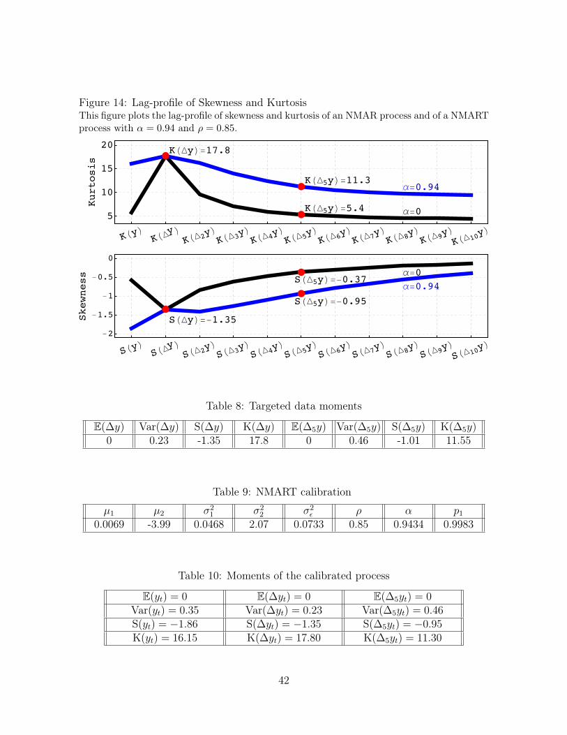
Figure 14: Lag-profile of Skewness and KurtosisThis figure plots the lag-profile of skewness and kurtosis of an NMAR process and of a NMARTprocess with α = 0.94 and ρ = 0.85.

�(Δ�)=��

�(Δ��)=��

�(Δ��)=�� α=�

α=��

�(�)

�(Δ�)

�(Δ��)�(Δ�

�)�(Δ�

�)�(Δ�

�)�(Δ�

�)�(Δ�

�)�(Δ�

�)�(Δ�

�)�(Δ�

��)

�

��

��

��

��

�(Δ�)=-��

�(Δ��)=-��

�(Δ��)=-��α=�

α=��

�(�)

�(Δ�)

�(Δ��)�(Δ�

�)�(Δ�

�)�(Δ�

�)�(Δ�

�)�(Δ�

�)�(Δ�

�)�(Δ�

�)�(Δ�

��)

-�

-��

-�

-��

�

��

Table 8: Targeted data moments

E(∆y) Var(∆y) S(∆y) K(∆y) E(∆5y) Var(∆5y) S(∆5y) K(∆5y)0 0.23 -1.35 17.8 0 0.46 -1.01 11.55

Table 9: NMART calibration

µ1 µ2 σ21 σ2

2 σ2ε ρ α p1

0.0069 -3.99 0.0468 2.07 0.0733 0.85 0.9434 0.9983

Table 10: Moments of the calibrated process

E(yt) = 0 E(∆yt) = 0 E(∆5yt) = 0Var(yt) = 0.35 Var(∆yt) = 0.23 Var(∆5yt) = 0.46S(yt) = −1.86 S(∆yt) = −1.35 S(∆5yt) = −0.95K(yt) = 16.15 K(∆yt) = 17.80 K(∆5yt) = 11.30

42

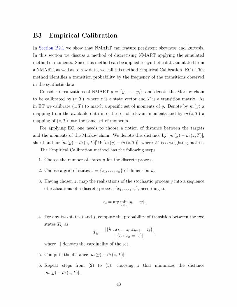
B3 Empirical Calibration

In Section B2.1 we show that NMART can feature persistent skewness and kurtosis.In this section we discuss a method of discretizing NMART applying the simulatedmethod of moments. Since this method can be applied to synthetic data simulated froma NMART, as well as to raw data, we call this method Empirical Calibration (EC). Thismethod identifies a transition probability by the frequency of the transitions observedin the synthetic data.

Consider t realizations of NMART y = {y1, . . . , yt}, and denote the Markov chainto be calibrated by (z, T ), where z is a state vector and T is a transition matrix. Asin ET we calibrate (z, T ) to match a specific set of moments of y. Denote by m (y) amapping from the available data into the set of relevant moments and by m̂ (z, T ) amapping of (z, T ) into the same set of moments.

For applying EC, one needs to choose a notion of distance between the targetsand the moments of the Markov chain. We denote this distance by |m (y)− m̂ (z, T )|,shorthand for [m (y)− m̂ (z, T )]′W [m (y)− m̂ (z, T )], where W is a weighting matrix.

The Empirical Calibration method has the following steps:

1. Choose the number of states n for the discrete process.

2. Choose a grid of states z = {z1, . . . , zn} of dimension n.

3. Having chosen z, map the realizations of the stochastic process y into a sequenceof realizations of a discrete process {x1, . . . , xt}, according to

xs = arg minw∈z|ys − w| .

4. For any two states i and j, compute the probability of transition between the twostates Tij as

Tij =|{h : xh = zi, xh+1 = zj}|

|{h : xh = zi}|,

where |.| denotes the cardinality of the set.

5. Compute the distance |m (y)− m̂ (z, T )|.

6. Repeat steps from (2) to (5), choosing z that minimizes the distance|m (y)− m̂ (z, T )|.

43

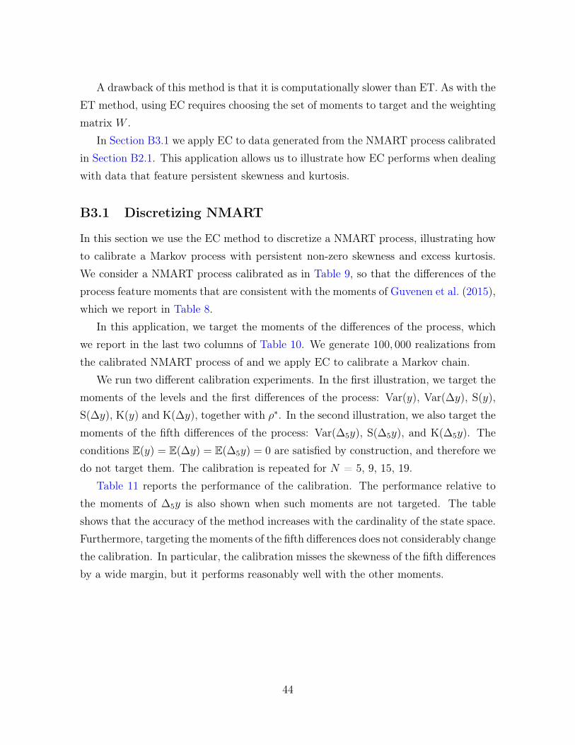
A drawback of this method is that it is computationally slower than ET. As with theET method, using EC requires choosing the set of moments to target and the weightingmatrix W .

In Section B3.1 we apply EC to data generated from the NMART process calibratedin Section B2.1. This application allows us to illustrate how EC performs when dealingwith data that feature persistent skewness and kurtosis.

B3.1 Discretizing NMART

In this section we use the EC method to discretize a NMART process, illustrating howto calibrate a Markov process with persistent non-zero skewness and excess kurtosis.We consider a NMART process calibrated as in Table 9, so that the differences of theprocess feature moments that are consistent with the moments of Guvenen et al. (2015),which we report in Table 8.

In this application, we target the moments of the differences of the process, whichwe report in the last two columns of Table 10. We generate 100, 000 realizations fromthe calibrated NMART process of and we apply EC to calibrate a Markov chain.

We run two different calibration experiments. In the first illustration, we target themoments of the levels and the first differences of the process: Var(y), Var(∆y), S(y),S(∆y), K(y) and K(∆y), together with ρ∗. In the second illustration, we also target themoments of the fifth differences of the process: Var(∆5y), S(∆5y), and K(∆5y). Theconditions E(y) = E(∆y) = E(∆5y) = 0 are satisfied by construction, and therefore wedo not target them. The calibration is repeated for N = 5, 9, 15, 19.

Table 11 reports the performance of the calibration. The performance relative tothe moments of ∆5y is also shown when such moments are not targeted. The tableshows that the accuracy of the method increases with the cardinality of the state space.Furthermore, targeting the moments of the fifth differences does not considerably changethe calibration. In particular, the calibration misses the skewness of the fifth differencesby a wide margin, but it performs reasonably well with the other moments.

44

Table 11: Empirical Calibration, AR(1) MixtureThis table shows the performance of the Empirical Calibration method when applied to aNMART process. We report the results for different cardinalities of the state space, N . Inpanel (1) of this table, we report the performance of EC when skewness and kurtosis of the fifthdifferences are not targeted. In panel (2) we report the performance of EC when skewness andkurtosis of the fifth differences are targeted. In the last two rows of the table, we report theaverage percentage absolute deviation from the targets: (%) denotes the average that excludesthe moments of the fifth differences, and (%∆5) denotes the average that includes them.

(1) (2)

∆5 moments not targeted ∆5 moments targeted

N 5 9 15 19 5 9 15 19ρ̂∗

ρ∗ 0.901 0.957 0.979 0.986 0.884 0.957 0.989 0.988Var(x)Var(y) 0.970 0.990 0.996 0.992 0.953 0.977 0.999 0.988S(x)S(y) 1.166 1.031 0.994 0.994 1.138 1.077 1.096 0.998K(x)K(y) 1.043 1.018 0.996 0.969 1.135 1.042 1.065 0.982

Var(∆x)Var(∆y) 1.179 1.083 1.041 1.023 1.194 1.068 1.023 1.014S(∆x)S(∆y) 0.327 0.820 0.890 0.907 0.585 0.831 0.994 0.927K(∆x)K(∆y) 0.666 0.869 0.902 0.903 0.742 0.891 1.015 0.928

Var(∆5x)Var(∆5y) 1.375 1.336 1.322 1.312 1.330 1.317 1.283 1.300S(∆5x)S(∆5y) 0.114 0.398 0.487 0.497 0.271 0.414 0.487 0.525K(∆5x)K(∆5y) 0.812 0.762 0.734 0.719 0.855 0.774 0.681 0.726

(%) 21.8 7.09 4.06 3.88 18.6 7.59 3.09 2.90

(%∆5) 29.7 16.7 13.9 13.7 25.1 16.6 13.3 12.5

45

Documents

Discretizing a Process with Non-zero Skewness and High ... · of a model depend crucially on this choice, calibrating the process and its discrete approximationdemandsgreatcare. Thankstotheirtractability,AR(1