Discretization errors and free surface stabilization in ...jupiter.ethz.ch/~tgerya/reprints/2011_G3_Thibault.pdf · ested in the deformation modes both prefailure and postfailure

Article

Volume 12, Number 7

8 July 2011

Q07004, doi:10.1029/2011GC003567

ISSN: 1525‐2027

Discretization errors and free surface stabilization in the finitedifference and marker‐in‐cell method for appliedgeodynamics: A numerical study

T. Duretz, D. A. May, T. V. Gerya, and P. J. TackleyInstitute of Geophysics, Department of Earth Sciences, ETH Zürich, Zurich CH‐8093, Switzerland([email protected])

[1] The finite difference–marker‐in‐cell (FD‐MIC)method is a popularmethod in thermomechanical modelingin geodynamics. Although no systematic study has investigated the numerical properties of the method,numerous applications have shown its robustness and flexibility for the study of large viscous deformations.The model setups used in geodynamics often involve large smooth variations of viscosity (e.g., temperature‐dependent viscosity) as well large discontinuous variations in material properties (e.g., material interfaces).Establishing the numerical properties of the FD‐MIC and showing that the scheme is convergent adds rele-vance to the applications studies that employ this method. In this study, we numerically investigate the dis-cretization errors and order of accuracy of the velocity and pressure solution obtained from the FD‐MICscheme using two‐dimensional analytic solutions. We show that, depending on which type of boundary con-dition is used, the FD‐MIC scheme is a second‐order accurate in space as long as the viscosity field is constantor smooth (i.e., continuous). With the introduction of a discontinuous viscosity field characterized by a vis-cosity jump (h*) within the control volume, the scheme becomes first‐order accurate. We observed that thetransition from second‐order to first‐order accuracy will occur with only a small increase in the viscosity con-trast (h* ≈ 5). We have employed two methods for projecting the material properties from the Lagrangianmarkers onto the Eulerian nodes. The methods are based on the size of the interpolation volume (4‐cell,1‐cell). The use of a more local interpolation scheme (1‐cell) decreases the absolute velocity and pres-sure discretization errors. We also introduce a stabilization algorithm that damps the potential oscillationsthat may arise from quasi free surface calculations in numerical codes that employ the strong form of theStokes equations. This correction term is of particular interest for topographic modeling, since the surface ofthe Earth is generally represented by a free surface. Including the stabilization enables physically meaningfulsolutions to be obtained from our simulations, even in cases where the time step value exceeds the isostaticrelaxation time. We show that including the stabilization algorithm in our FD stencil does not affect the con-vergence properties of our scheme. In order to verify our approach, we performed time‐dependent simulationsof free surface Rayleigh‐Taylor instability.

Components: 14,800 words, 14 figures, 3 tables.

Keywords: convergence; finite difference; free surface; marker‐in‐cell.

Index Terms: 0545 Computational Geophysics: Modeling (1952, 4255, 4316); 0560 Computational Geophysics: Numericalsolutions (4255); 3225 Mathematical Geophysics: Numerical approximations and analysis (4260).

Received 16 February 2011; Revised 6 May 2011; Accepted 7 May 2011; Published 8 July 2011.

Duretz, T., D. A. May, T. V. Gerya, and P. J. Tackley (2011), Discretization errors and free surface stabilization in the finitedifference and marker‐in‐cell method for applied geodynamics: A numerical study, Geochem. Geophys. Geosyst., 12,Q07004, doi:10.1029/2011GC003567.

Copyright 2011 by the American Geophysical Union 1 of 26

http://dx.doi.org/10.1029/2011GC003567

1. Introduction

1.1. Background

[2] Unravelling the deformation history from thepresent‐day geological record is a challenging prob-lem. To complement field data and traditional inter-pretation based geodynamic modeling approaches,mathematical models are often employed to developour understanding of geological processes. The useof thermomechanical models which solve the equa-tions of conservation ofmomentum,mass and energyhas a long history in geodynamics.

[3] In these models one prescribes (1) a set ofmathematically permissible boundary conditions,(2) the geometry of the model domain, and (3) thegeometry and rheology (or lithology) of the rocksto be modeled. Using such an approach to simulategeologically realistic scenarios is complicated byseveral attributes which we discuss in more detail.At a given length scale, rocks can be extremelyheterogenous. Here, the heterogeneities may con-sist of differing lithology, or in simply the contrastof effective material properties (viscosity, shearmodulus, etc). Furthermore, the contrast of effectivematerial propertiesmay be extremely large, and occurover a very small length scale. The geometry of theheterogeneities is also a complex issue to treat inthermomechanical models as coherent structures(e.g., layering) may need to be represented. Overgeological time scales, rocks are subjected to enor-mous strains, i.e., large deformation. Given thatrocks possess characteristics of both ductile andbrittle materials (over a certain time scale), duringtheir deformation they will yield. In contrast tomany engineering applications, geologists are inter-ested in the deformation modes both prefailure andpostfailure.

[4] This set of physical attributes associated withgeological processes has motivated numerous dif-ferent modeling approaches. Rather than describeall the methods in detail, we instead provide a briefhistorical overview of the approaches and highlightthe merits and shortcomings with regards to thephysical attributes identified above. Two broad cat-egories of methods can be defined: (a) those whichexplicitly models interfaces from which a materialdomain (volume) is inferred or (b) those whichexplicitly model volumes.

[5] We refer to van Keken et al. [1997], Popov andSobolev [2008], Zlotnik et al. [2007], Braun et al.[2008], Samuel and Evonuk [2010], Schmalzl and

Loddoch [2003], and Lin and van Keken [2006]as examples of methods from category (a). Whilemany methods to represent interfaces exist, devel-oping robust schemes with low numerical diffusion,and which are capable to representing complexstructures required by geodynamic models is non-trivial. With the advent of affordable, distributedmemory computer clusters, it is also an importantconsideration whether a given method can beimplemented in 3‐D and whether the algorithm issuitable to be implemented in a distributed memoryenvironment.

[6] For geological applications, the geometric com-plexity of the structure needing to be represented,combined with algorithmic difficulties associatedwith implementing interface based models, hasmotivated the use of “particle based” methods(category (b)). The term “particles” is deliberatelyused vaguely as different methods may regard“particles” in different ways. In general, particlesare used to represent a given lithology (i.e., materialproperties) and as such represent volumetric quan-tities. The huge advantage afforded by particlemethods is that they are completely unstructured,and do not posses any connectivity associated withneighboring particles. The use of particles to trackcomplex flow features (e.g., free surface evolution)dates back to the pioneering marker‐and‐cell (MAC)method [Harlow and Welch, 1965; Pracht, 1971].Here, the particles (or markers) were Lagrangianquantities and were used to represent (discretize) thevolume of the fluid. The fluid equations for con-servation of mass and momentum were solved viaa staggered grid, finite difference method. Themarkers were used to indicate which cells in thegrid were completely filled with fluid, and whichcontained the free surface, and hence where the freesurface boundary condition should be applied. TheMAC methodology has been extensively developedin the geodynamics community [Weinberg andSchmeling, 1992; Poliakov and Podladchikov,1992; Zaleski and Julien, 1992; Fullsack, 1995;Tackley, 1998;Babeyko et al., 2002;Gerya and Yuen,2003, 2007;Moresi et al., 2003, 2007]. These authorsfollow the underlying concept introduced in theMAC scheme. Namely, the conservation equationsare solved on a grid, while complex geometric fea-tures are represented with markers. In the geo-dynamic applications, the markers are not usedsimply to identify regions of free surface/fluid/air,rather they typically represent different lithologiesto which material parameters and a constitutivelaw is attributed. Other Lagrangian particle based

GeochemistryGeophysicsGeosystems G3G3 DURETZ ET AL.: FD‐MIC SCHEME DISCRETIZATION ERRORS 10.1029/2011GC003567

2 of 26

methods used in geodynamics include Poliakovet al. [1993], Braun and Sambridge [1994, 1995],Hansen [2003], and Schwaiger [2007]. While dif-ferent in their methodology, they embody Harlow’soriginal concept.

[7] The idea of representing complex geometricstructures via Lagrangian markers is very appeal-ing, and consequently gained widespread usage incomputational geodynamics for a number of rea-sons: it is very simple to associate lithology andmaterial properties to markers; the numerical imple-mentation of marker fields is algorithmically straightforward; three‐dimensional implementations ofmarker methods are not significantly more complexthan its 2‐D counterpart; the approach is amenableto distributed memory environments.

1.2. Present Work

[8] To obtain reliable results from numericalmodels, one has to ensure that a sufficiently high“numerical resolution” is used to guarantee thatthe physics is captured. Depending on the method,numerical resolution might be related to the sizeof grid cell used in a mesh, or the number of markersused to represent a volume of fluid. Furthermore,one has to establish that the numerical error associ-ated with the method used actually decreases if theresolution is increased. That is, the convergence ofthe method must be established. Understanding theconvergence properties of a method provides someinsight into the resolution required to resolve a cer-tain flow feature (for example) and furthermore, italso indicates how rapidly the error is reduced as afunction of increasing numerical resolution.

[9] Despite the widespread usage and acceptanceof thermomechanical modeling as a viable tool tostudy geology, few studies focus on the accuracyof the numerical methods being employed. In gen-eral, it is often regarded that it is difficult to performa formal error analysis on marker based methodsdue to their inherent unstructured nature. Further-more, geological applications often utilize discon-tinuous material properties (e.g., viscosity). The useof spatially variable coefficients also make formalerror analysis more complicated. While the marker‐grid methods lack a formal error analysis, numerousnumerical studies have been performed. Numericalstudies consist of either output comparison betweendifferent codes or laboratory experiments (a.k.a.benchmark studies) [Blankenbach et al., 1989; Traviset al., 1990; van Keken et al., 1997; Tackley andKing, 2003; Buiter et al., 2006; Schmeling et al.,

2008; OzBench et al., 2008; van Keken et al.,2008], or solution comparison between an analyticsolution and the model output [Moresi et al., 1996;Deubelbeiss and Kaus, 2008; Popov and Sobolev,2008; Zhong et al., 2008].

[10] Given the number of practitioners nowemploying marker grid style thermomechanicalnumerical models, it is important to thoroughlyaddress the order of convergence of these methods,either through carefully designed numerical experi-ments or analytical approaches [Nicolaides, 1992;Nicolaides and Wu, 1996]. In this work, we con-sider one such representative marker grid basedapproach [Gerya and Yuen, 2003, 2007] andnumerically examine the convergence propertiesof the method. This is achieved by using threedifferent analytic solutions for a Stokes flow prob-lem with continuous and discontinuous viscositystructures. Although idealized, these solutions havesufficient complexity in terms of their lithology andgeometry to be regarded as representative of a typ-ically geodynamic application. Using the analyticsolutions, the true discretization error can be mea-sured. While using analytic solutions to measureerrors and determine the order of convergence isby no means exhaustive (in a mathematical sense),in the absence of formal convergence proof, theapproach is justified if the analytic solutions possesssufficient complexity compared to the intendedapplication of interest. Given the interest in re-presenting free surfaces for modeling topographyand the difficulties that are related to the intro-duction of this surface [Kaus et al., 2010], we adopta strong form variant of the stabilization techniquedescribed by Kaus et al. [2010] for a finite dif-ference scheme. To verify that the use of this algo-rithm does not affect the convergence propertiesof our finite difference–marker‐in‐cell scheme(FD‐MIC), we again utilize analytic solutions.

[11] The outline of this paper is as follows. In thefirst section we introduce the physical problem ofinterest along with the numerical method that weemploy. In section 3 we describe the sources oferrors and the methodology we employ to analyzethe discretization error of our numerical method.The models used in the convergence study and theresults obtained using the convergence propertiesof the FD‐MIC method are described in thesection 4. Section 5 provides an application of ourmethod to solve a time‐dependent free surfaceproblem. In section 6 we discuss some futuredirections and perspectives beyond examining dis-


3 of 26

cretization errors within numerical schemes. Lastly,concluding remarks are provided in section 7.

2. Physical Problem and NumericalMethod

2.1. Governing Equations

[12] Traditionally, the flow of geomaterials overgeological timescales is calculated by solving themomentum equations neglecting inertial terms(Stokes equations)

@�ij@xj

¼ ��gi: ð1Þ

This equation describes the balance between theviscous force and the body forces for an infini-tesimal volume of fluid. The viscous force is for-mulated as the gradient of the stress tensor (sij)and the body force is written as the product of thefluid density (r) and the gravitational accelerationvector (gi). Moreover, in the absence of meltingand phase transitions, geodynamic flows are con-sidered as incompressible. Incompressibility isenforced by coupling the aforementioned equationswith the continuity equation

@vi@xi

¼ 0; ð2Þ

where vi is the velocity and xi is the spatial coordi-nate. Equations (1) and (2) are valid over the modeldomain which we denote by W. To close the systemthe equations for the conservation of momentum andmass are supplemented with two boundary condi-tions. Decomposing the boundary of W into two,nonoverlapping regions denoted by ∂WN and ∂WD,the boundary conditions are written as

�ijnj ¼ ai; x 2 @WN ð3Þ

and

vi ¼ bi; x 2 @WD: ð4Þ

Here nj is the outward point normal to the boundaryof W, ai is an applied traction and bi is a prescribedvelocity.

[13] The mechanical behavior of the material isdefined by a constitutive relationship. We relate thestress tensor sij to the strain rate tensor _�ij, using alinear, isotropic viscous rheology given by

�ij ¼ �p�ij þ 2� _�ij; ð5Þ

where p is the pressure, h is the viscosity and thestrain rate is given by

_�ij ¼ 1

2

@vi@xj

þ @vj@xi

� �: ð6Þ

[14] The model domain contains several differentmaterial compositions, or lithologies which wedenote by C(x). The compositional field C doesnot possess any physical diffusion, and evolvesaccording to

@C

@tþ vi

@C

@xi¼ 0: ð7Þ

[15] Prior to any discretization, the equations aboveare nondimensionalized by means of dynamicscaling. This scaling is achieved by first defining aset of characteristic units such as a characteristiclength (e.g., domain size), a characteristic time(e.g., diffusion time, inverse background strain rate),a characteristic viscosity (e.g., minimum viscosityin the domain) and secondly deriving all the relatedcharacteristic units (mass, stress, force..). In section 4,we employ characteristic units that are equal to 1.The results are not scaled back to dimensional unitsand therefore the velocity errors and pressure aredimensionless. The experiment described insection 5 involves processes occurring at Earth‐like dimensions and thus the characteristic unitsdiffer from 1, the corresponding results are scaledback to dimensional units.

2.2. Numerical Method

2.2.1. Spatial Discretisation

[16] We solve equations (1) and (2) for the primi-tive variables vi and p. The discrete solution of thetwo field formulation is defined by a grid basedconservative finite difference scheme. The con-straint imposed by incompressibility condition iseffectively treated using the classical staggered gridarrangement of the primitive variables [Harlowand Welch, 1965]. In the staggered formulationused here, we solve for pressure which is definedat cell centers and for the component of velocitynormal to the cell face Figure 1). The velocitycomponent is located at the centroid of each cellface. For flow problems possessing a spatially var-iable viscosity, the viscosity is required to bedefined at both the vertices, and the center of eachcontrol volume, in order for the discrete equationsto conserve stress between neighboring control


4 of 26

volumes [Patankar, 1980]. This particular staggeredgrid difference scheme has been demonstrated to berobust in solving variable viscosity problems inmantle convection by numerous authors [Ogawaet al., 1991; Tackley, 1993; Ratcliff et al., 1995;Harder and Hansen, 2005; Trompert and Hansen,1996; Stemmer et al., 2006; Tackley, 2008] and inlithospheric dynamics [Zaleski and Julien, 1992;Gerya and Yuen, 2003, 2007; Katz et al., 2007].

[17] The material properties viscosity and densityare discretized in space via a set of markers, orparticles. For a given property � represented via themarker field, we adopt the following interpolantdefined on the markers

� xð Þ � �m xð Þ ¼XNmp¼1

� x� xp� �

�mp ; ð8Þ

where �pm is the value of property � (viscosity or

density) defined at marker p, Nm is the number ofmarkers, d(x − xp) denotes the standard Kroneckerdelta function and the marker coordinate is xp. Forsimplicity we express equation (8) via

�m xð Þ ¼ QT xð ÞFm; ð9Þ

where Fm is the vector of all marker values used torepresent the field � and QT is a row vector witheach entry defining the Kronecker delta functionfor each marker p.

[18] To evaluate the finite difference stencil, we arerequired to interpolate the marker values for vis-cosity and density onto the relevant locations (cellvertex or centroid) within the FD grid. Here wederive the “marker‐to‐node” interpolation schemedefined by Gerya and Yuen [2003] by regarding theoperation as an L2 projection (least squares mini-mization) of the marker properties onto the verticesof a structured grid. To derive the interpolant in thestudy by Gerya and Yuen [2003], we first definegrid based representation of the field �. The grid isconstructed from vertices of the cells defining eachpressure control volume. Over each cell, the gridrepresentation of field, which we denote by �g(x),is assumed to vary according to a bilinear function.Denoting the bilinear interpolant at node i by Ni(x),we have the following approximation for � over thegrid

� xð Þ � �g xð Þ ¼XNni¼1

Ni xð Þ�gi

¼ NT xð ÞFg;

ð10Þ

Figure 1. Spatial distribution of the primitive variables (u, v, p) and material properties (h, r) for a two‐dimensionalstaggered grid and example of boundary conditions discretizations (case of the u momentum equation). The blacksymbols represent the nodes that are part of the stencil for the boundary equation discretization. The gray symbolsrepresent the neighboring nodes that are not taken into account in the stencil. (a) The extrapolated boundary conditionis formulated as a linear combination of two internal u nodes. (b) The fictitious node boundary condition implemen-tation is achieved by discretizing the equations along the domain boundary. The dashed symbol represent the fictivepoint used for the formulation of this boundary equation.


5 of 26

where Nn is the number of vertices in the mesh, Fg

is the vector of all nodal values used to representthe field � and NT is a row vector with each entrydefining the interpolation function Ni(x) for node i.The interpolating functions Ni have a compactsupport bW, implying the functions are only nonzeroover a subset of the entire domain W. In this work,the compact support of each interpolant Ni, is bW ≡2Dx × 2Dy, where Dx, Dy are the cell dimensionsin the x and y direction, respectively. Furthermore,the grid interpolants Ni are a partition of unity, that

isPNni¼1

Ni(x) = 1. In Figure 2a we depict the compact

support for a node i (denoted by the gray region)

and the shape of the bilinear interpolation functionNi. Outside of the gray region, Ni(x) = 0.

[19] The projection operator P can be defined as

P : �m xð Þ ! �g xð Þ:

Given that the number of markers and vertices inthe mesh is not equal, a natural choice to define Pis to use the L2 projection of �m onto �g. The leastsquares minimization leads us to seek a solution ofthe following:

min1

2

ZW

�g xð Þ � �m xð Þð Þ2dV� �

¼ min J½ �; ð11Þ

Figure 2. The “4‐cell” and “1‐cell” schemes for projecting properties defined on the markers (denoted by stars) ontoa node (denoted by the solid circle). (a) The 4‐cell scheme. The support of the interpolating function Ni associatedwith node i is indicated by the shaded region. Only markers within the support of node i contribute to the projectionoperation used to define the nodal value at i. The shape of the bilinear interpolation function for node i is indicated inthe lower frame. (b) The 1‐cell scheme. The thick lines in the lower frame indicate the grid used to discretize theStokes equations, while the thin lines indicate the grid onto which marker properties are projected. The 1‐cell schemeutilizes a compact support of size Dx × Dy. The support for nodes r, s, t are indicated by the shaded regions. Onlymarkers within the nodal support contribute to the projection operation for that node. The vertex and cell centeredvalues on the grid used to discrete Stokes equations (points r and s, respectively) are directly obtained from the localprojection scheme.


6 of 26

where W is the model domain. Substitutingequations (9) and (10) into equation (11) andcomputing ∂J/∂Fg = 0 we obtain

ZWN xð ÞNT xð ÞdV

� �Fg ¼

ZWN xð ÞQT xð ÞFmdV ; ð12Þ

and inserting equation (8) yields

ZWN xð ÞNT xð ÞdV

� �Fg ¼

XNm

p¼1

N xp� �

�mp : ð13Þ

[20] The “marker‐to‐node” interpolation of Geryaand Yuen [2003] is obtained from equation (13)by making the following approximations; (1) repla-cing the matrix on the left hand side by a diagonalmatrix defined by summing the entries in eachrow, i.e.,

Ni xð ÞNj xð Þ � Ni xð ÞXNnk¼1

Nk xð Þ !

�ij

¼ Ni xð Þ�ij;ð14Þ

where the summation in brackets was eliminatedsince Ni form a partition of unity and (2) evaluatingthe integrals using a numerical quadrature definedby the markers within the compact support of eachNi. ApproximatingNNT by a diagonal matrix makesthe projection operation completely local to eachnode i in the mesh. This choice is predominatelymade to reduce the computational cost by eliminat-ing the need to solve a matrix problem. Neverthe-less, it is usually more desirable to utilize a local L2approximation, as global L2 tend to produce overlysmooth fields. Given that the interpolant used for themarker fields are Kronecker delta functions (seeequation (9)), the most natural quadrature scheme touse is a Monte Carlo method in which the markerscoordinates define the abscissa of the quadraturescheme and every quadrature point is assigned thesame quadrature weight, with the only constraint thatthe sum of the weights should equal the volume of theintegration domain. Incorporating the above two as-sumptions, and invoking equation (9) reducesequation (12) to the following:

�gi ¼

PNm

p¼1Ni xp� �

�mp

PNm

p¼1Ni xp� � : ð15Þ

[21] We note that the L2 interpolant defined inequation (12) wasO(h2) accurate, where h representsthe grid spacing, as the function space onto whichwe projected the marker field was bilinear. How-ever, the approximated interpolant in equation (15)possesses a reduced rate due to the choice of quad-rature scheme utilized. In the worst case, classicalMonte Carlo quadrature with random abscissaconverges like O(n−1/2), where n is the number ofpoints, while quasi Monte Carlo methods usingpseudo random abscissa can converge as fast asO(

ffiffiffiffiffiffiffiffiffiffiffiffiffilog nð Þp

/n). The abscissa used in our quad-rature scheme are determined via the coordinates ofthe markers, which are inherently nondeterministicand are the result of the solution to Stokes flow.Consequently, we anticipate that the quadrature ruleemployed here will tend toward the classical MonteCarlo limit and thus the expected order is O(H1/2),where H is the average spacing of the markers. Inthis work, the projection depicted in Figure 2awill be referred to as the “4‐cell” scheme.

[22] In the study by Gerya and Yuen [2007], a“local” variant of the projection operator inequation (12) was proposed. This local marker‐to‐node projection is depicted in Figure 2b. Theprincipal difference is that the marker properties areprojected onto a grid of finer resolution (thin lines,bottom frame) than the grid used to discretizeStokes equations (thick lines, bottom frame), thusthe compact support of each interpolant Ni is nowbW ≡ Dx × Dy. While developed heuristically,numerical experiments revealed that this local pro-jection method yielded more accurate results [Geryaand Yuen, 2007]. Given that we have shown that theinterpolant used by Gerya and coworkers is anapproximate L2 projection, it is apparent why thelocal variant yields more accurate results. Specifi-cally, we note that while the order of the local L2projection is the same variant depicted in Figure 2a,the discretization parameter h has been reduced bya factor of two, which thus also reduces the error.In the local projection scheme, vertex values andcell center values (denoted by r and s, respectively,in Figure 2b) are obtained from application ofequation (15) on the finer grid. Note that themidside values (denoted by t) are not required bythe finite difference stencil. The projection depictedin Figure 2b will be referred to as the “1‐cell”scheme.

2.2.2. Temporal Discretisation

[23] The Lagrangian markers are used to discretizeeach composition field C. In the Lagrangian frame


7 of 26

of reference, the solution of equation (7) can beobtained by solving the following two equations:

DCp

Dt¼ 0;

dxpdt

¼ vp; ð16Þ

where Cp, xp, vp are the composition, coordinateand velocity vector of marker p, respectively. Thesolution of DCp/Dt = 0 is trivially obtained with themarker representation. The kinematic equation issolved using a fourth‐order Runge‐Kutta (RK4)time stepping scheme applied to each marker p. Wedo not reevaluate the flow field during the appli-cation of RK4, thus the method is fourth‐orderaccurate in space only. The velocity field at themarker vp, is obtained by interpolating the flowfield computed on the finite difference grid to themarker coordinate xp. After the markers have beenadvected, the material properties are interpolatedfrom the new marker positions to the Eulerian gridusing either the 4‐cell or 1‐cell projection definedby equation (15). Alternatively, higher‐order timeintegrators such as the predictor‐corrector methodare employed in the community [Weinberg andSchmeling, 1992; Schmeling et al., 2008], thismethod achieves second‐order (in time) accuracybut requires to solve the discrete Stokes equationstwice per time integration.

2.2.3. Boundary Condition Implementation

[24] We have used two different techniques toimpose boundary conditions (BC) on the non–boundary matching nodes of the staggered grid.The first method (extrapolated boundary condition)enables to describe the stress or velocity value atthe boundary by setting a condition on two nodesinside the domain (extrapolation). A linear combi-nation of the velocities at those two nodes defines avelocity gradient, the value of the velocity at theboundary is therefore set by the value of the gra-dient. For instance the u component of a free slipboundary condition at the top of the domain(assuming zero normal velocity) is expressed as

@u

@y

top

¼ 0¼) uC � uS ¼ 0; ð17Þ

where the node labeling is depicted in Figure 1. Forthe no slip case, we extrapolate to the boundary, thus

ujtop¼ 0¼) uC � 1

3uS ¼ 0: ð18Þ

[25] The stencil corresponding to this boundaryequation only contains two points and additional

constraints are needed while solving for pressure.This condition is usually fulfilled by setting addi-tional pressure constrain such as zero horizontalpressure flux in the corners of the domain [Gerya,2010]. Given the fact that the boundary condition isdefined via extrapolation, we expect this imple-mentation to be first order in space. A secondmethod (fictitious node method) is derived bydiscretizing the momentum equations along thedomain boundaries. The usual stencil is modified toaccount for “virtual nodes” outside of the domain.These virtual nodes are used to define the velocityflux at the boundary of the domain, they are notexplicitly included into the system of equations.The isoviscous u momentum equation stencil at thetop of the domain is written as

@�xx@x

þ �uF þ uS � 2uC

Dy2

� �þ �

@2v

@y@x� @p

@x¼ ��gx; ð19Þ

with

uF ¼ uC ; ð20Þ

for a free slip case and

uF ¼ �uC ; ð21Þ

for a no slip case.

[26] This method do not require any additionalpressure constrains, thus no boundary conditions arerequired while solving for pressure. With this dis-cretization of the boundary condition, each partialderivative is approximated bymeans of central finitedifferences and we therefore expect this method tobe second‐order accurate in space.

2.2.4. Free Surface Treatment

[27] As shown byKaus et al. [2010], the introductionof a free surface boundary condition in geodynamicsimulations can induce artificial numerical oscilla-tions in the free surface. This phenomena was coinedthe “drunken seaman” instability. The free surface inthese models represents an interface between air androck, and this is characterized by a sharp jump indensity (∼103 kg.m−3). A large displacement of thisinterface within a single time step can therefore giverise to severe “out‐of‐balanceness” [Kaus et al.,2010]. Physically, this imbalance may occur whenthe employed time step exceeds the isostatic relax-ation time [Fuchs et al., 2011]. Such a situation islikely to occur when an explicit advection scheme isused, since the nonlinear residual associated with theadvected coordinates (at time t + Dt), and the eval-uation of the force term and stresses (at time t) is not


8 of 26

guaranteed to be small. The “drunken seaman”instability can occur when the free surface is explic-itly tracked, such as in a body fitted Lagrangian finiteelement method, or when the free surface boundarycondition is approximated via the “sticky air”approach [Schmeling et al., 2008], which is com-monly used in Eulerian‐Lagrangian finite differencemethods in which explicit meshing of the interfaceis not possible. Several methods can be used tostabilize the evolution of the free surface, whicheither involve solving the nonlinearity related toadvection or introducing higher‐order terms arisingfrom a Taylor series expansion of the momentumbalance equation. Here we focus on the secondapproach applied to our staggered grid finite differ-ence discretization.

[28] Kaus et al. [2010] showed that a higher‐orderTaylor series expansion of the weak formulationof the momentum balance equation leads to anexpression of a correction term which has the formof a boundary traction. This correction term is thendiscretized and added to the original Stokes stiff-ness matrix. Following this methodology, wederive a similar correction term for the strong formof the Stokes equations (such as used with thefinite difference method) by performing a Taylorseries expansion of equation (1) about the pointx + �Dtv, whereDt is the time step and 0 < � < 1 isan arbitrary parameter used to limit the size of thedisplacement increment. The expansion of the stresstensor sij, is given by

�ij xþ �Dtvð Þ � �ij xð Þ þ �Dt vk �ij xð Þ �;kþO Dt2ð Þ; ð22Þ

where the subscript , k denotes a partial derivativewith respect to xk. The gradient of the stress tensorsij,j, is then

�ij;j xþ �Dtvð Þ � �ij;j xð Þ þ �Dt vk �ij xð Þ �;jk

þ �Dt vk;j �ij xð Þ �;kþO Dt2

� �: ð23Þ

Assuming that g is constant, we expand the densityas

� xþ �Dtvð Þ � � xð Þ þ �Dt vk � xð Þ½ �;kþO Dt2ð Þ: ð24Þ

Inserting equations (23) and (24) into equation (1)and keeping only the terms which are linear in vkand those of O(Dt), we obtain the perturbedmomentum balance equation

�ij;j xð Þ þ �Dt � xð Þ;kvk gi ¼ �� xð Þgi: ð25Þ

Here, the term �Dt r(x),k vk represents a higher‐order correction which is a function of the velocity

field, vk. We denote the discrete representation of themomentum equation in equation (25) via

Kuþ LuþGp ¼ f ; ð26Þ

whereKu is discrete gradient of the stress tensor,Gpis the discrete pressure gradient, f is the discretebody force and Lu is the stabilization term. Theconstruction of L requires the current time step Dtand the evaluation of the density gradient at each ofthe u, v nodes. In our FD‐MIC formulation, this isachieved by central finite differences. We evaluate@�@x ≈

D�Dx and

@�@y ≈

D�Dy at the u and v nodes, respectively.

The first‐order derivatives are computed usingvalues of density defined at the cell center (i.e., atthe pressure node). The density at the cell centeris interpolated from the marker density field, oraveraged from a density field defined on thevertices of the grid.

3. Discretization Errorsand Convergence

3.1. Errors in Approximate Solutionsof PDEs

[29] Errors in the approximate solution of partialdifferential equations (PDEs) arise from four mainsources.

[30] 1. The discretization error (or truncation error),which is defined as the difference between a givenmathematical model (analytic solution) and its dis-cretized expression. In the case of the finite differencemethod, the derivative of a function is numericallyestimated by first assuming that the function is con-tinuous, and then by replacing the continuous deriv-ative with a truncated Taylor series about a point.The discretization error is therefore generated by thetruncation of the Taylor expansion and is propor-tional to the remainder (O(hn)). This type of dis-cretization error is termed a locally generated errorby Roy [2010].

[31] 2. An additional discretization error may occurin the definition of the coefficients within the PDE.Coefficients may consist of terms on the right sideof the equation (e.g., density), or terms within thedifferential operator itself (e.g., viscosity). Coeffi-cients will possess a discretization error if they areobtained by interpolation (e.g., projection of markersproperties to nodes), or if they are a function ofvariables which were discretized. Typical examplesof the latter include temperature or strain rate–dependent viscosity where temperature (or velocity)are discretized over a grid, and the viscosity is


9 of 26

required at a location which doesn’t coincide with adiscretization point in the grid.

[32] 3. Roundoff errors arising from the numericalrepresentation of real, continuous numbers, with afinite precision representation. This error thereforedepends on the precision (number of digits) whichis employed to represent floating point numbers ina numerical scheme.

[33] 4. The error resulting from the solution ofsystems of linear equations.The use of direct solvers (such as LU, Choleskydecomposition) can minimize this type error, at leastto the extent possible with finite precision arithmetic(see item 3 above). However, if iterative methods areused, the error induced is a result of stopping con-dition used to terminate the iterative cycle. Robuststopping conditions should monitor the residualassociated with the system and the current estimateof the solution. However, one still needs to specify ameasure of when the residual is “small enough” toconclude that the iterative method has converged.

[34] We here focus on the evaluation of the dis-cretization error of the FD‐MIC scheme. Our spe-cific interest is to determine the convergence of themethod in the case where viscosity jumps (discon-tinuous coefficients) occur at a subgrid level. Thediscretization error of the FD‐MIC scheme can beseen as the combination of the truncation error ofthe staggered grid (including boundary conditiondiscretization) and the error related to the projec-tion of material properties onto the nodes. In thisstudy, the discrete system of equations describingStokes flow was solved using a direct factorizationtechnique, thus eliminating any error associated withusing an iterative method. All calculations wereperformed using double precision arithmetic.

3.2. Measuring Convergenceof the Discretization: Methodology

[35] Several methods are available in order to studythe discretization error of numerical schemes[Roache, 1997; Roy, 2010]. We here focus onmeasuring the order of convergence of the primitivevariables of our discrete Stokes problem. To do so,we employed two‐dimensional analytic solutionswhich can be utilized to determine the exact velocityand pressure values at each node of our grids. Inorder to compute the discretization error, we utilizethe L1 norm, which for a scalar quantity �, is definedas follows:

k�k1¼ZW�j jdV ; ð27Þ

where W is the model domain. For a vector quantityw = (s, t) we have

kwk1 ¼ ksk1 þ ktk1¼ZW

sj j þ tj jð ÞdV : ð28Þ

We define the pressure error as

kepk1 :¼ kp� pexactk1; ð29Þ

where pexact is the exact value of the pressure. The L1error for the velocity u = (u, v), is defined via

keuk1 :¼ keuk1 þ kevk1 ¼ ku� uexactk1 þ kv� vexactk1;ð30Þ

where uexact and vexact are the exact values of the u,v velocity components. For numerical computationswe approximate the above integrals via a one pointquadrature rule, i.e.,

k�k1 � k�kh1 :¼Xe

� xeð Þj j Ve; ð31Þ

where Ve is the representative volume for thepoint xe. For FD schemes, the appropriate volumeto use in equation (31) is the control volume asso-ciated with each node. Within staggered grid FDschemes, the control volume associated with the pand u, v degrees of freedom are different. In ourresults, we utilize two‐dimensional meshes contain-ingM ×M elements. As a result, we have (M + 1) ×Mnodes for u, M × (M + 1) nodes for v, and M × Mnodes for pressure. From this, we define the follow-ing discrete L1 norm for pressure as

kpk1 �XMI¼1

XMJ¼1

pI ;J DxDy; ð32Þ

where DxDy is the cell volume For the velocitycomponents we have

kuk1 � 1

2

XMJ¼1

u1;J DxDyþ

XMI¼2

XMJ¼1

uI ;J DxDy

þ 1

2

XMJ¼1

u Mþ1ð Þ;J DxDy; ð33Þ

kvk1 � 1

2

XMI¼1

vI ;1 DxDyþ

XMI¼1

XMJ¼2

vI ;J DxDy

þ 1

2

XMI¼1

vI ; Mþ1ð Þ DxDy: ð34Þ

[36] The order of convergence of the discretizationis determined by computing the numerical solutiondefined on a sequence of uniformly refined grids,


10 of 26

and computing the L1 norm of eu and ep on eachgrid. Following this, a least squares regression isperformed on the log10 of the error norm and thecell size h. We relate the convergence rate of the L1norms for velocity and pressure errors to the orderof convergence via

keuk1 � Chru ; kepk1 � Chrp ; ð35Þ

where h is the mesh size, C is a constant inde-pendent of the grid resolution h, and ru, rp are theorder of convergence for velocity and pressurefields, respectively. In all our experiments, the gridpossesses the same number of vertices N in eachdirection. We define our grid sequence using N ={41, 81, 101, 201, 301, 401, 501, 601, 701, 801,901, 1001}.

4. Numerical Experiments

4.1. Idealized Models Usedin the Convergence Study

[37] To study the error distributions and conver-gence properties of our numerical scheme, we car-ried out two sets of experiments. Each of these testsis aimed at studying the effect of a spatially variablecoefficient (viscosity) on the discretization. Wedefine a global measure of the viscosity contrastover the entire domain W via h* = max(h(x))/min(h(x)). The first test focuses on the buoyancy‐drivenflow in a box containing a one‐dimensional vis-cosity structure. The second test addresses theinfluence of a large but smooth variation of viscositywithin a box where the flow is driven by buoyancy.The third test investigates a pure shear deformationfield, which is perturbed by the presence of a two‐dimensional, circular, highly viscous inclusion.

4.1.1. One‐Dimensional Viscosity Structure:SolCx

[38] The first series of convergence test were per-formed using a two‐dimensional analytical solutionof a variable viscous Stokes flow problem whichwe identify as SolCx. The model domain is definedas W ≡ [0, 1] × [0, 1]. The boundary conditions onall sides of the domain are prescribed to be freeslip, implying that the normal velocity to each wallis zero, and the tangential stress along the wallvanishes. Internal to the domain, fluid flow isdriven by a sinusoidal force given by

F ¼ 0;� sin yð Þ cos xð Þð ÞT : ð36Þ

In practice this force is imposed by setting a con-stant gravity acceleration (x component equal to 0and y component equal to 1) and the allowing thedensity field to vary in space according to

� x; yð Þ ¼ sin yð Þ cos xð Þ: ð37Þ

Experiments were carried out for both isoviscousand variable viscosity case, in the latter case theviscosity field is discontinuous and is given by

� x; yð Þ ¼1; if 0 � x � 0:5

106; if 0:5 < x � 1:

8<: ð38Þ

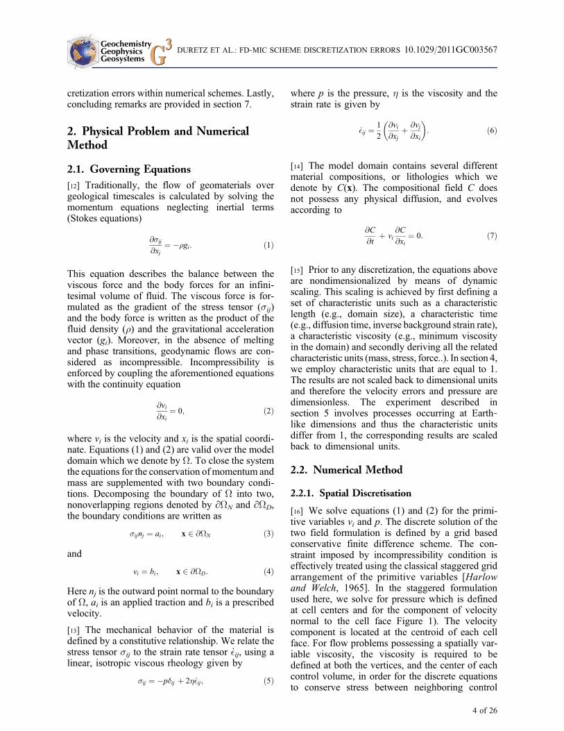
This setup allows for sharp viscosity jumps of largemagnitude which is a typical requirement for geo-dynamic applications (see Figure 3). Furthermore,the discontinuous viscosity structure provides amore challenging test of both the discretization andthe solver in comparison to solutions with contin-uous viscosity structures. A complete description ofthe analytic solution is provided by Zhong [1996].The source code used in our study to evaluate theanalytic solution is available from the open sourcepackage Underworld [Moresi et al., 2007]. Since theflow is driven by the density gradients, we will againuse this test to analyze the influence of the freesurface stabilization scheme on the convergence ofthe FD‐MAC method.

4.1.2. Smooth Viscosity Variation in OneDimension: SolKz

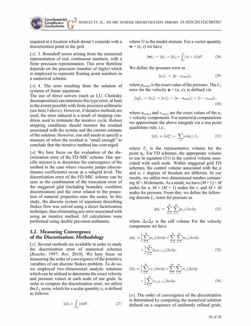
[39] In order to investigate the effect of a large andsmooth viscosity variation on our discretization, weutilized the analytic solution from Revenaugh andParsons [1987], which here we have termedSolKz. This solution allows for a exponential vari-ation of viscosity from the bottom to the top of themodel domain which is defined asW ≡ [0, 1] × [0, 1].All the boundaries are free slip and the flow is drivenby a smooth density distribution, the forcing termis expressed as

F ¼ 0;� sin 2yð Þ cos 3xð Þð ÞT : ð39Þ

and the viscosity increases from the bottom to thetop of the box according to

� yð Þ ¼ exp 2Byð Þ ð40Þ

with the parameter B controlling the magnitude ofthe overall viscosity variation. Here we choose Bsuch that over the vertical extend of the domain wehave viscosity contrast of Dh* = 106. The density,


11 of 26

viscosity distribution and the resulting flow fieldare depicted in Figure 4. Similarly to the SolCxtest, the source code used to evaluate the analyticalsolution is part of the open source packageUnderworld.

4.1.3. Two‐Dimensional Viscosity Structure:Pure Shear Inclusion Test

[40] The third series of convergence test were carriedout using the analytical solution for an inclusion in a

Figure 4. Density (r), viscosity (h), and flow pattern (u, v, p) for the analytic solution SolKz.

Figure 3. Material properties and the analytic solution for SolCx. The r and h are the density and viscosity distribu-tions, u, v are the analytic x, y components of velocity, respectively, and p is the analytic pressure field. The verticalcomponent of gravity acceleration is 1.


12 of 26

weak matrix undergoing pure shear. The derivationas well as the scripts that can be used to computethe analytic are available in the study by Schmid[2002] and Schmid and Podladchikov [2003]. Forthis problem, the model domain is defined as W ≡[−1, 1] × [−1, 1] and contains a circular shapedinclusion at the origin. The inclusion has a radius,Rinc of 10% the length of the domain. The viscosityfield is given by

� x; yð Þ ¼1; if x2 þ y2 > Rinc

2

103; if x2 þ y2 � Rinc2;

8<: ð41Þ

as used by Deubelbeiss and Kaus [2008]. The flowis driven by a pure shear strain rate boundary con-

dition and the force vector, rgi is zero (Figure 5).In this test, the circular shape of the inclusionensures that the viscosity jump is never alignedwith cartesian coordinate system, and thus is neveraligned via the finite difference stencil. Conse-quently, this test is particularly relevant sincebodies of arbitrary shape (e.g., plumes, slabs)typically develop during the evolution of geody-namic simulations.

4.2. Staggered Grid Discretization

[41] In the first set of experiments, we used the ana-lytical solution SolCx to examine the convergenceproperties of the staggered grid finite difference

Figure 5. Viscosity structure (h) and analytic solution for velocity (u, v) and pressure (p), for the pure shear inclusiontest [Schmid and Podladchikov, 2003]. For this setup, the flow is driven by a strain rate boundary condition ( _� = 1),and the buoyancy forcing term is 0 (e.g., r = 0 or gy = 0).


13 of 26

discretization These experiments do not employmarkers to represent the material properties h, r.The finite difference stencil was thus definedby directly evaluating equations (36) and (38).Experiments were performed using the two differ-ent boundary condition implementations describedin section 2.2.3.

4.2.1. SolCx: Isoviscous

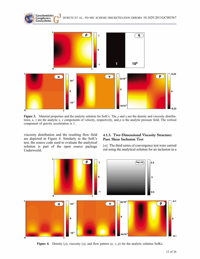
[42] Here we consider a spatially constant viscosityfield, i.e., h(x, y) = 1. These tests were performed inorder to measure convergence of the method for anoptimal case, and to assess the error associated withthe different boundary condition implementations.In Figure 6, the error distribution for a 101 × 101grid resolution is shown. A clear influence of thetype of boundary condition can be observed. Withboth implementations, the maximum error for allfields is confined along the boundary of the domain.However, the error obtained using the extrapolatedBC approach is significantly larger. At this resolu-tion, we observe that the velocity and pressure errorsare approximately 2 orders of magnitude smallerwhen the fictitious node BC implementation isused. The L1 errors for a sequence of grid resolu-tions is shown in Figure 7a, and the computed ratesare provided in Table 1. As we expected, the

velocity and pressure obtained using extrapolatedBC discretization converge to the analytical solu-tion with a rate of ∼1. The fictitious node boundarycondition implementation yields u, p fields whichboth converge at a rate of ∼2. From Figure 7a, it isapparent that the absolute value of the velocity andpressure errors in L1 are much lower (for all gridresolutions) when the fictitious node BC is used.Given these results, we will refer to extrapolatedBC method and the fictitious node BC imple-mentation as the “first‐order” and “second‐order”BC methods in the following sections.

4.2.2. SolCx: 106 Viscosity Jump

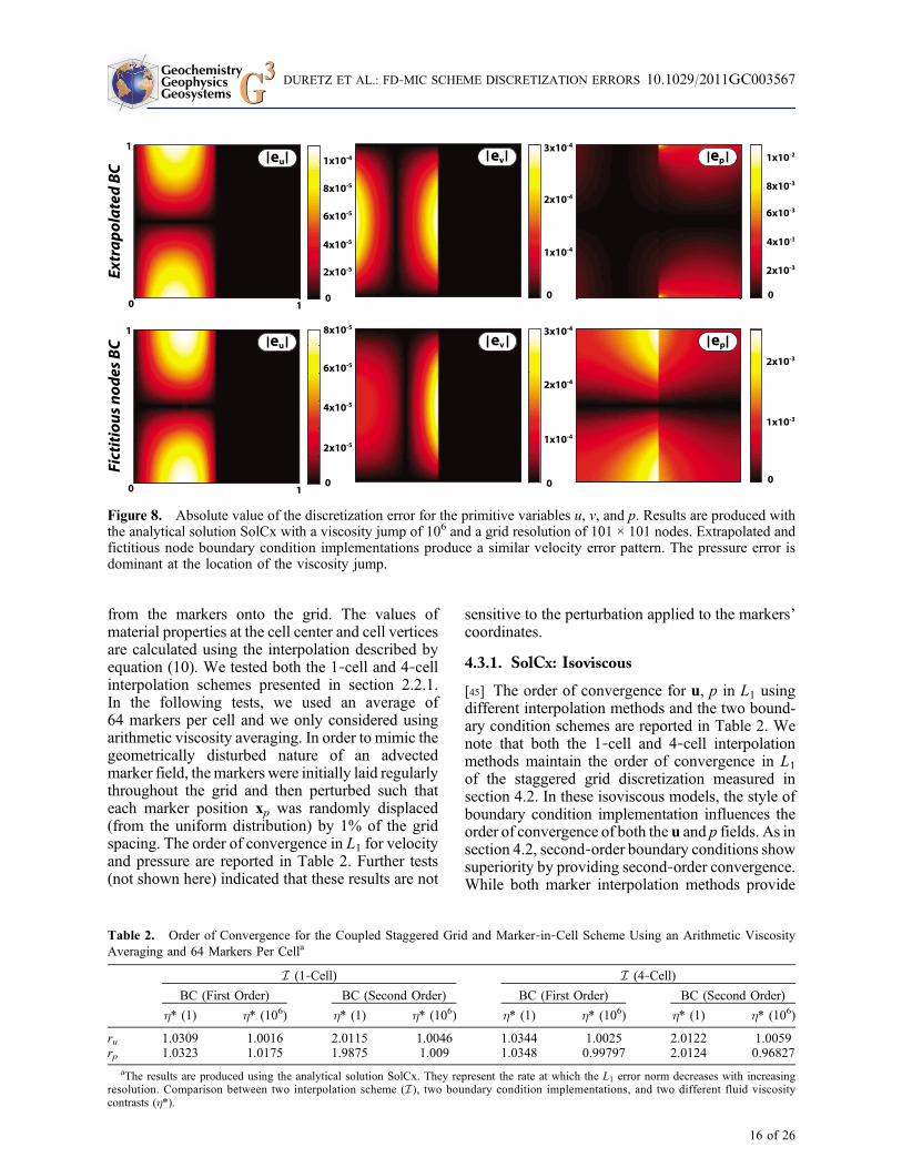
[43] In this second test, a large discontinuous jumpin viscosity (106 Pa.s) was introduced. The dis-cretization error for a 101 × 101 grid resolution isshown Figure 8. In comparison with the isoviscousresults (Figure 6), the location of the maximumerror is no longer only confined along the boundaryof the domain. Rather, we now observe that max-imum errors in u, v occur within the low‐viscosityregion, and share a similar spatial correlation withthe isoviscous case if we consider only the low‐viscosity domain (x < 1

2). For the v velocity com-ponent, the maximum absolute error is located atthe jump, with a magnitude of ∣ev∣ ≈ 10−4 for both

Figure 6. Spatial distribution of the absolute value of the discretization error (eu, ev, ep) for the variables u, v, and p.Comparison between extrapolated and fictitious node boundary condition implementations. Maximum errors arelocated at the domain boundaries. The error pattern and magnitudes between the two methods are notably different.The test was carried out using the isoviscous SolCx setup with a grid resolution of 101 × 101 nodes.


14 of 26

boundary condition implementations. The effect ofthe BC implementation remains visible for both uand v, at the boundaries second‐order BC produceserrors which are approximately 1 order of magni-tude smaller than for the first‐order case. Pressureerrors are distributed at the jump and close to theboundaries. In contrast with the isoviscous case, thepressure errors are much larger than the velocityerrors (≈10–100 times) and significantly larger(≈100–1000 times) than in the isoviscous case. Thediscontinuous variation of the viscosity not onlyhas a strong influence on the spatial distribution oferrors, but also on the order of convergence ofthe computed velocity and pressure fields. The L1errors for the variable viscosity case are shown inFigure 7b, and the computed rates are providedin Table 1. The most noticeable feature is that thechoice of boundary condition implementation ismuch less critical. This is apparent as we observethat the convergence of the velocity and pressureerrors in L1, for both boundary condition im-plementations, are approximately first order. Themagnitudes of the L1 error for velocity and pressureerror are lower when using second‐order boundaryconditions, however the difference is less than 0.25of an order of magnitude. For this particular test, weobserved different results if an even grid sequencewas employed. The even grid sequence correspondsto a situation where the central pressures nodes arelocated directly on the viscosity jump. Using an even

grid sequence with second‐order boundary condi-tions lead to an improvement of the velocity andpressure errors in L1, with orders of convergence ofru = 2.0 and rp = 1.0, respectively. Due to the superconvergent nature of these rates, we regard mesheswith viscosity jumps aligned with pressure nodes asa special case. While it is of interest to understandthe reason for the apparent super convergentbehavior, in practice we rarely ever encountermaterial property contrast which can be aligned withthe grid, thus we do not study this special case anyfurther here.

4.3. Staggered Grid and Marker‐in‐CellDiscretization

[44] In the second set of experiments, we definedthe material properties (h, r) via markers, thereforeboth viscosity and density fields were projected

Figure 7. Velocity and pressure L1 error norms with increasing resolution for the SolCx test. Viscosity and densityare directly sampled, and therefore no interpolation is used. (a) First‐order convergence is achieved while usingextrapolated boundary conditions. Second‐order convergence is obtained with fictitious node boundary conditions.(b) As soon as a jump in viscosity is introduced, both extrapolated and fictitious node boundary conditions convergeat a first‐order rate.

Table 1. Order of Convergence of the L1 Error NormBetween Analytics and Numerics Without Using Interpolationa

BC (First Order) BC (Second Order)

h* (1) h* (106) h* (1) h* (106)

ru 1.0648 1.0052 2.0276 1.0064rp 1.0416 1.0026 2.0297 1.0114

aResults are produced using the analytical solution SolCx.Comparison between two boundary condition implementations.Results are calculated for two different fluid viscosity contrasts.


15 of 26

from the markers onto the grid. The values ofmaterial properties at the cell center and cell verticesare calculated using the interpolation described byequation (10). We tested both the 1‐cell and 4‐cellinterpolation schemes presented in section 2.2.1.In the following tests, we used an average of64 markers per cell and we only considered usingarithmetic viscosity averaging. In order to mimic thegeometrically disturbed nature of an advectedmarker field, themarkers were initially laid regularlythroughout the grid and then perturbed such thateach marker position xp was randomly displaced(from the uniform distribution) by 1% of the gridspacing. The order of convergence in L1 for velocityand pressure are reported in Table 2. Further tests(not shown here) indicated that these results are not

sensitive to the perturbation applied to the markers’coordinates.

4.3.1. SolCx: Isoviscous

[45] The order of convergence for u, p in L1 usingdifferent interpolation methods and the two bound-ary condition schemes are reported in Table 2. Wenote that both the 1‐cell and 4‐cell interpolationmethods maintain the order of convergence in L1of the staggered grid discretization measured insection 4.2. In these isoviscous models, the style ofboundary condition implementation influences theorder of convergence of both the u and p fields. As insection 4.2, second‐order boundary conditions showsuperiority by providing second‐order convergence.While both marker interpolation methods provide

Figure 8. Absolute value of the discretization error for the primitive variables u, v, and p. Results are produced withthe analytical solution SolCx with a viscosity jump of 106 and a grid resolution of 101 × 101 nodes. Extrapolated andfictitious node boundary condition implementations produce a similar velocity error pattern. The pressure error isdominant at the location of the viscosity jump.

Table 2. Order of Convergence for the Coupled Staggered Grid and Marker‐in‐Cell Scheme Using an Arithmetic ViscosityAveraging and 64 Markers Per Cella

I (1‐Cell) I (4‐Cell)

BC (First Order) BC (Second Order) BC (First Order) BC (Second Order)

h* (1) h* (106) h* (1) h* (106) h* (1) h* (106) h* (1) h* (106)

ru 1.0309 1.0016 2.0115 1.0046 1.0344 1.0025 2.0122 1.0059rp 1.0323 1.0175 1.9875 1.009 1.0348 0.99797 2.0124 0.96827

aThe results are produced using the analytical solution SolCx. They represent the rate at which the L1 error norm decreases with increasingresolution. Comparison between two interpolation scheme (I ), two boundary condition implementations, and two different fluid viscositycontrasts (h*).


16 of 26

similar rates of convergence, 1‐cell interpolation ismore accurate than 4‐cell for a given number ofmarker per interpolation volume (Figure 9a). In thistest, the viscosity field is spatially constant, thus thedifference in error is therefore related to the inter-polation of density (a smooth field in this model)required to assemble the force vector. The offsetsbetween the velocity and pressure solutions with andwithout introducing marker‐to‐node interpolation is∼0.5 an order of magnitude.

4.3.2. SolCx: 106 Viscosity Jump

[46] In Figure 9b the errors for a sequence of gridresolutions used to solve the variable viscosity caseare provided. Similarly to the test in section 4.2.2in which no marker‐to‐node interpolation wasemployed, all the simulations converged with arate of first order for velocity and pressure, regard-less of the type of interpolation used. The choice ofusing either 1‐cell or 4‐cell interpolation method forinterpolating the viscosity jump and the smoothlyvarying density field only appeared to affect theaccuracy of the pressure field.

4.3.3. SolKz: 106 Smooth Viscosity Variation

[47] We have run the test SolKz to test the effect ofa large continuous variation of viscosity through

the domain. We have used second‐order boundaryconditions and two interpolation methods. Second‐order L1 velocity and pressure convergence wereobtained while using 1‐cell interpolation. 4‐cellinterpolation provided second‐order velocity con-vergence and a pressure convergence order rp,slightly less than 2. For this particular test, theabsolute velocity and pressure error are approxi-mately half an order of magnitude more accuratewhen the 1‐cell method is utilized (Figure 10).

4.3.4. Inclusion Test: 103 Viscosity Jump

[48] This analytical solution requires a strain rateboundary condition (e.g., pure shear) to be appliedfar away from the center of the domain where theinclusion is located. In order to avoid any problemsrelated to the treatment of this particular boundarycondition, each boundary was treated as a Dirichletboundary. The analytical solution was evaluatedand imposed on the boundaries of our modeldomain. This approach also has the effect ofremoving the truncation error introduced whilediscretizing the strain rate boundary condition.

[49] The tests were run for an inclusion/bulk vis-cosity contrast of 103, using both the first‐order andsecond‐order boundary condition implementations.Nodal material properties were evaluated from the

Figure 9. Velocity and pressure L1 norms for SolCx test. Comparison of different material properties interpolationsschemes (4‐cell, 1‐cell). Results are obtained using 64 markers per interpolation area. For this specific test, we usedsecond‐order BC. (a) With an isoviscous problem, velocity and pressure errors converge at second order. The offsetsbetween the different lines are a result of the density interpolation. For similar marker density per interpolation vol-ume, local interpolation provides more accurate results. (b) When a viscosity jump is introduced, all solutions con-verge at a first‐order rate. The influence of the interpolation scheme is only noticeable on the pressure error.


17 of 26

marker field using 1‐cell and 4‐cell interpolationsand both interpolations were carried out using anaverage of 64 markers per interpolation volume.Given the sharp, two‐dimensional viscosity struc-ture (circular), this setup provides a tough test forboth the discretization and the interpolationscheme. For all our cases, we obtained first‐orderconvergence in L1 for the velocity and pressurefields (Table 3).

4.3.5. Free Surface Stabilization

[50] In this section, we investigate the influencethat the free surface stabilization scheme describedin section 2.2.4 has on the order of convergence ofthe staggered grid discretization. For this purpose,we used the test SolCx described in section 4.1.1.This test does not include a free surface, but sincethe flow is driven by density gradients, the contri-

bution of the stabilizing terms in the discretizationis therefore nonzero. In order to choose the value ofthe time step, here we evaluate the time step using aCourant criteria (with � = 0.5) computed from thegrid spacing and the maximum velocities givenby the analytical solution. In practice, for time‐dependent problems, the value of the time step usedwould be that computed from the flow field andmesh configuration from the previous time step.

[51] We ran a convergence test using the second‐order boundary condition implementation and 1‐cellinterpolation (64 markers per interpolation volume)with a viscosity jump of 106. The stabilizationaffects the spatial distribution of error (compareFigure 11a with Figure 8). This affect is related tothe proportionality between the magnitude of thecorrection term and the density gradients. Withdecreasing grid spacing, the numerical scheme withstabilization conserves its first‐order convergence

Figure 10. Dependance of L1 velocity and pressure error norms on the grid spacing (h) for the SolKz test. We testedtwo different material properties interpolation (4‐cell, 1‐cell) with a fixed number of markers per interpolation volume(64). Second‐order BC discretization were employed.

Table 3. Order of Convergence for Velocity and Pressure for the Inclusion Test (h* = 103), Using the Staggered Grid andMarker‐in‐Cell Scheme Employing an Arithmetic Viscosity Averaging and 64 Markers Per Cella

I (1‐Cell) I (4‐Cell)

BC (First Order) BC (Second Order) BC (First Order) BC (Second Order)

ru 1.025 0.94897 1.0634 1.0043rp 0.98051 0.94107 0.99427 0.94204

aThe order of convergence are observed to be independent of the type of marker‐to‐node interpolation and the style of boundary conditionimplementation.


18 of 26

in L1 for both velocity and pressure, although aslight offset in pressure convergence was observedbetween simulations including or not the stabili-zation (dashed lines Figure 11b). Therefore thestabilization term does not noticeably modify theflow discretization, nor the overall convergence ofthe method.

5. Application to a Rayleigh‐TaylorInstability With a Free Surface

[52] In section 4.3.5, we applied the free surfacestabilization algorithm to the model setup of SolCxand observed that the order of convergence wasunaltered by the introduction of the stabilization.We considered this test as being suitable for aconvergence test, even though the problem doesnot include a free surface, as the flow is driven by

buoyancy, thus possesses spatial variations in den-sity. In order to test the robustness of the free surfacestabilization scheme presented in section 2.2.4, weran several simulations of a Rayleigh‐Taylor insta-bility with a free surface. This setup was used byKaus et al. [2010] and was shown to produce the“drunken seaman” instability with a finite elementcode which explicitly tracked the free surface. Withour Eulerian‐Lagrangian approach, we approximatethe free surface by using “sticky air”, i.e., weintroduce a layer of zero density, low‐viscosityincompressible material [Schmeling et al., 2008].The pseudo free surface is then defined as theinterface between the crust and the “sticky air”,which is free to deform. The setup of the exper-iment consists of a domain W ≡ [−250, 250] ×[−600, 0] km, with a resolution of 502 cells (Dx =10 km, Dy = 12 km). The box is filled with a400 km thick asthenosphere, a 100 km thick layer

Figure 11. (a) Spatial distribution of the absolute value of the discretization error including the stabilization algo-rithm. (b) Influence of the stabilization algorithm on the convergence of the staggered grid and marker‐in‐cell discre-tization. The results were produced using the second‐order BC and 1‐cell interpolation (64 markers per cell); the setupincludes a viscosity jump of 106. Dashed and solid lines are pressure and velocity L1 convergence, respectively.Crosses represent the results obtained with the stabilization; squares are the reference results without stabilization.


19 of 26

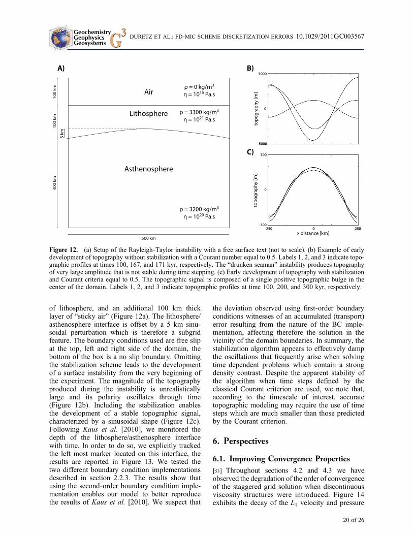
of lithosphere, and an additional 100 km thicklayer of “sticky air” (Figure 12a). The lithosphere/asthenosphere interface is offset by a 5 km sinu-soidal perturbation which is therefore a subgridfeature. The boundary conditions used are free slipat the top, left and right side of the domain, thebottom of the box is a no slip boundary. Omittingthe stabilization scheme leads to the developmentof a surface instability from the very beginning ofthe experiment. The magnitude of the topographyproduced during the instability is unrealisticallylarge and its polarity oscillates through time(Figure 12b). Including the stabilization enablesthe development of a stable topographic signal,characterized by a sinusoidal shape (Figure 12c).Following Kaus et al. [2010], we monitored thedepth of the lithosphere/asthenosphere interfacewith time. In order to do so, we explicitly trackedthe left most marker located on this interface, theresults are reported in Figure 13. We tested thetwo different boundary condition implementationsdescribed in section 2.2.3. The results show thatusing the second‐order boundary condition imple-mentation enables our model to better reproducethe results of Kaus et al. [2010]. We suspect that

the deviation observed using first‐order boundaryconditions witnesses of an accumulated (transport)error resulting from the nature of the BC imple-mentation, affecting therefore the solution in thevicinity of the domain boundaries. In summary, thestabilization algorithm appears to effectively dampthe oscillations that frequently arise when solvingtime‐dependent problems which contain a strongdensity contrast. Despite the apparent stability ofthe algorithm when time steps defined by theclassical Courant criterion are used, we note that,according to the timescale of interest, accuratetopographic modeling may require the use of timesteps which are much smaller than those predictedby the Courant criterion.

6. Perspectives

6.1. Improving Convergence Properties

[53] Throughout sections 4.2 and 4.3 we haveobserved the degradation of the order of convergenceof the staggered grid solution when discontinuousviscosity structures were introduced. Figure 14exhibits the decay of the L1 velocity and pressure

Figure 12. (a) Setup of the Rayleigh‐Taylor instability with a free surface text (not to scale). (b) Example of earlydevelopment of topography without stabilization with a Courant number equal to 0.5. Labels 1, 2, and 3 indicate topo-graphic profiles at times 100, 167, and 171 kyr, respectively. The “drunken seaman” instability produces topographyof very large amplitude that is not stable during time stepping. (c) Early development of topography with stabilizationand Courant criteria equal to 0.5. The topographic signal is composed of a single positive topographic bulge in thecenter of the domain. Labels 1, 2, and 3 indicate topographic profiles at time 100, 200, and 300 kyr, respectively.


20 of 26

convergence order with increasing viscosity con-trast. Here we observe a reduction of the conver-gence, from second order to first order, when theviscosity contrast is increased from one (isoviscous)to ten. These results were obtained using the analyticsolution SolCx. While these results are representa-tive of a one‐dimensional viscosity structure, thistype of behavior is commonly observed whensolving problems involving large discontinuities incoefficients [Das et al., 1994], or waves such asthose occurring in shock dynamics [Banks et al.,2008], where shocks behaves as discontinuitiesand locally reduce the order of convergence of thenumerical scheme. Restoring the optimal conver-gence properties of numerical method, prior to theintroduction of the discontinuities is appealing. Herewe briefly describe some efforts toward this.

[54] In section 4.2.2 we noted that under a specificalignment of our finite difference grid with the one‐dimensional discontinuous viscosity structure, theoptimal order of convergence for our method wasobserved. While this was regarded as a “special”case, it does raise the question, under what con-ditions is the viscosity jump correctly captured byour FD stencil? It has been proposed that differ-ent averaging methods (harmonic, geometric) ofmaterial properties can lead to improved numericalresults [MacKinnon and Carey, 1988; Das et al.,1994]. Examples of using such methods for vis-cous flow problems are available in the literature[Das et al., 1994; Deubelbeiss and Kaus, 2008;Schmeling et al., 2008], however, determining

which averaging scheme is appropriate remainsunsolved. The conclusions to this questions differwith the various model setup (boundary drivenflow, buoyancy driven flow, viscosity contrast) andwith the structure of the discontinuity (1‐D versus2‐D versus 3‐D geometries). While such averagingis completely justified in 1‐D problems, it does notnaturally generalize to higher dimensions andconsequently is not robust enough for general use.Additionally, the aforementioned averaging meth-ods only consider scalar quantities, or isotropicconstitutive tensors. The extension of the approachto tensorial quantities, which may be required forobtaining an effective stress, or an effective or-thotropic constitutive tensor is nontrivial. We referto Cowin and Yang [1997] for further details onthis topic.

[55] In contrast to rudimentary averaging of mul-tiscale behavior (or coefficients), homogenizationprovides an alternative view by decomposingphenomena into two scales: a macroscale (coarsescale) and a microscale (fine scale). The essence ofthis class of methods is to extract coarse scaleequations (or coefficients) which incorporate amultitude of different scales. The idea of scaleseparation can be naturally adopted to the FD‐MICscheme discussed here, in which we have a modeldomain discretized via cells (coarse scale) andwithin each cell we have numerous markers whichdefine variations of the viscosity and density,thereby describing fine scale information. In clas-sical homogenization theory [Bensoussan et al.,

Figure 13. Free surface evolution during the Rayleigh‐Taylor instability test as presented by Kaus et al. [2010]. Wemonitor the vertical coordinate of a marker initially positioned on the lithosphere/asthenosphere boundary and next tothe left side of the box. Results are all computed for a Courant number equal to 0.5. Differences can been seenbetween the first‐order and second‐order boundary condition implementations; the latter follows the results [Kauset al., 2010] more closely.


21 of 26

1978; Murat, 1978], it is frequently required toassume that the fine scale heterogeneity is periodicin one direction, thus this approach may lack thegenerality required. Nevertheless, further extensionsof classical homogenization are being developed fornonperiodic heterogeneities [Capdeville et al.,2010]. For a thorough review of homogenizationwe refer to Hassani and Hinton [1998a, 1998b,1998c]. Numerous alternatives to classical homog-enization exist [see, e.g., Brewster and Beylkin,1995; Abdulle and Weinan, 2003; Arbogast, 2002;Jenny et al., 2003; Weinan and Engquist, 2003;Kouznetsova et al., 2002]. These methods alsoemploy coarse and fine scale representation of theproblem, however they do not assume that the finestructure is periodic. Many of these methods requirethe solution of independent cell problems, wherelocal, fine scale solutions are subsequently coupledto a coarse grid solution. Such approaches couldused in geodynamic models to resolve fine scalestructure defined via the markers, and may alsoimprove the convergence [Masud and Khurram,2004; Liu and Li, 2006] of our scheme in the pres-ence of discontinuous viscosity fields.

6.2. Input Data Uncertainty Estimationand Model Parameter Sensitivity

[56] In the light of establishing that the numericalscheme employed to solve a given set of equations,which describes the geodynamic process of inter-

est, has been deemed to be sufficiently accurate androbust, other challenges await. Geodynamic simu-lations require prescription of the rheologicalbehavior and its associated parameters for eachlithology present in the system. In practice, theseparameters and flow laws are frequently derivedexperimentally. The evaluation of flow parametersat high pressure/temperature is a challenging taskand the behavior of crystals such as olivine at depthstill remains widely debated [Raterron et al., 2009;Rozel et al., 2011]. Moreover, the extrapolation offlow laws from laboratory time scales to geologicaltime scales give rise to additional uncertainties[Paterson, 1987]. One interesting direction forgeodynamic modeling is the integration of thematerial property uncertainties into the simulations,as done in other communities [Laz et al., 2007;Houtekamer et al., 1996; Rabier et al., 1996].

[57] Another avenue to explore could be to con-sider the geodynamic model as an “optimal design”problem [Hicks and Henne, 1978; Jameson, 1988,1995; Giles and Pierce, 2000]. In such approaches,one seeks to minimize (or maximize) a givenobjective function F, subject to set of design vari-ables U which define the model setup. For instance,in the context of a viscous folding model, thedesign parameters might be: size of the modeldomain, rheological parameters (viscosity, den-sity), rate of compression applied as a boundarycondition, and the objective function could be tominimize the difference between the dominant

Figure 14. Measured convergence rate of the staggered grid with increasing viscosity contrast (h*). Solid anddashed lines represent the convergence rate of the velocity and pressure measured in L1, respectively. The measure-ments were carried out using the analytic solution SolCx and the second‐order BC implementation. Projection ofmarker properties h, r was not used; these fields were evaluated on the FD stencil using equations (38) and (36).


22 of 26

wavelength from the model and one observed fromfield data. From such optimal design approaches,one obtains the relativity sensitivity of F withrespect to each design parameter Ui, or phrasedanother way, we can answer the question of what isthe perturbation in dominant wavelength due thedomain size, rheological parameters and boundarycondition. Both optimal design and the integrationof parameter uncertainties provide a means toquantitatively characterize model parameter sensi-tivities, thereby further developing our understand-ing of the system of equations we choose torepresent our geological problem.

7. Conclusions

[58] Computational modeling in geology requiresnumerical methods that are robust, reliable andaccurate when applied to study the deformation ofmaterials which possess discontinuities in theirproperties. Such variations in material parametersare likely to strongly influence the quality of thesolution. While theoretical analysis of such methodsis difficult due to the discontinuous nature of thematerial properties, very few numerical studiesfocussing specifically on the quality of discretesolutions obtained from geodynamic models havebeen performed. Quantifying the numerical accu-racy for complex models that are relevant to geo-dynamics is of vital importance if the solution are tobe used in any quantitative manner. In this study, weaddress these issues by examining the discretizationerrors and convergence characteristics of the dis-crete solution obtained from the FD‐MIC scheme,which is a widely utilized method in the geodynamiccommunity.

[59] The convergence study was carried out usingtwo‐dimensional analytical solutions which pos-sess large continuous and discontinuous variationsin the viscosity field. Two different boundaryconditions implementations, namely extrapolatedBC and fictitious nodes methods were tested. If thefluid was isoviscous, we found that the fictitiousnode method provided second‐order accurate veloc-ity and pressure fields and therefore showed supe-riority over the extrapolated BC method, whichproduced first‐order accurate fields. Smooth butlarge variations of viscosity throughout the modeldomain did not affect the second‐order behavior ofthe FD‐MIC method. However, the introductionof a viscosity jump in the model domain affectedthe convergence properties of the fictitious nodemethod, resulting in first‐order velocity and pressurefields. This drop in the order of convergence

occurred if the viscosity jump was larger than 5. Anessential component of our Eulerian‐Lagrangiandiscretizations is the projection of marker propertiesonto the finite difference grid. We tested two dif-ferent marker‐to‐node projections which differ intheir domain of influence. Introducing these pro-jections was not observed to modify the order ofconvergence of the FD‐MIC method. The morelocal 1‐cell interpolation was shown to be moreaccurate than the 4‐cell interpolation. For the rangeof problems considered, our results clearly estab-lish that the FD‐MIC scheme converges. That is,increases in the numerical resolution lead to areduction of the discretization error. Demonstratingthat the method is convergent adds robustness toboth previous and future geodynamic applicationswhich employ this particular numerical method.

[60] Additionally, we introduced a strong formvariant of the free surface stabilization algorithmpresented by Kaus et al. [2010]. This stabilizationmethod is suitable for finite difference discretiza-tions. By the means of a convergence test, weshowed that the stabilization algorithm also does notnotably affect the convergence properties of ournumerical scheme. Further testing was carried out byperforming time‐dependent simulations and using asetup which is prone to instability. This test dem-onstrated that the stabilization suppresses the insta-bility that may occur while running free surfacecalculations. The stabilization permits larger timesteps to be used. Whilst this certainly does notimprove the temporal accuracy of the solution, itsinclusion is necessary to obtain physically mean-ingful results from simulations which use a Couranttime step. The stabilization method is important forany simulation that includes large density contrasts.In our modeling, the surface of the Earth is a clas-sical example of this type of interface. Thus, thisstabilization routine approach is particularly rele-vant for modeling topography in regional and globalscale simulations over geological time periods.

[61] Lastly, we wish to remark that continuedresearch in understanding discretization errors andconvergence properties of the numerical tools usedto study geological processes is vitally important ifwe wish to develop the level of reliability androbustness in our modeling technology which existsin the engineering community. However, equally asimportant as the quality of our numerical solutions,is our ability to understand the dynamics of thesystem we use to describe geological processes, andthis entails understanding the sensitivity of themodel output to the underlying flow laws, material


23 of 26

parameters and boundary conditions and otherinput used to define our model.

Acknowledgments

[62] The authors thank Harro Schmeling and Cedric Thieulotfor constructive reviews that improved the quality and clarityof the paper. We also thank Jed Brown and Alban Souchefor useful discussions related to the free surface stabilizationand discretization errors. We thank Boris Kaus for constructiveinput and fruitful discussions related to errors and for provid-ing the Matlab script defining the analytical solution for theviscous inclusion test and data for the Rayleigh‐Taylor test.DAM acknowledges Mirko Vélic for producing the sourcecode used to evaluate the analytic solution, SolCx and SolKz.TD thanks la Tartouze for proofreading. TD was funded by theSNF‐EU research grant 20TO21‐120535 (TOPO‐4D). DAMwas supported by the ETH Zurich Postdoctoral FellowshipProgram.

References

Abdulle, A., and E. Weinan (2003), Finite difference heteroge-neous multi‐scale method for homogenization problems,J. Comput. Phys., 191, 18–39.

Arbogast, T. (2002), Implementation of a locally conservativenumerical subgrid upscaling scheme for two‐phase Darcyflow, Comp. Geosci., 6, 453–481.

Babeyko, A. Y., S. V. Sobolev, R. B. Trumbull, O. Oncken,and L. L. Lavier (2002), Numerical models of crustal‐scaleconvection and partial melting beneath the Altiplano‐Punaplateau, Earth Planet. Sci. Lett., 199, 373–388.

Banks, J. W., T. Aslam, and W. J. Rider (2008), On sub‐linearconvergence for linearly degenerate waves in capturingschemes, J. Comput. Phys., 227, 6985–7002.

Bensoussan, A., J. Lions, and G. Papanicolau (1978),Asymptotic Analysis for Periodic Structures, 700 pp.,North Holland, Amsterdam.

Blankenbach, B., F. Busse, U. Christensen, L. Cserepes,D. Gunkel, U. Hansen, H. Harder, G. Jarvis, M. Koch,G. Marquart, D. Moore, P. Olson, H. Schmeling, andT. Schnaubelt (1989), A benchmark comparison for mantleconvection codes, Geophys. J. Int., 98, 23–38.

Braun, J., and M. Sambridge (1994), Dynamical LagrangianRemeshing (DLR): A new algorithm for solving large straindeformation problems and its application to fault‐propagationfolding, Earth Planet. Sci. Lett., 124, 211–220.

Braun, J., and M. Sambridge (1995), A numerical method forsolving partial differential equations on highly irregularevolving grids, Nature, 376, 655–660.

Braun, J., C. Thieulot, P. Fullsack, M. DeKool, C. Beaumont,and R. Huismans (2008), DOUAR: A new three‐dimensionalcreeping flow numerical model for the solution of geologicalproblems, Phys. Earth Planet. Inter., 171(1–4), 76–91.

Brewster, M. E., and G. Beylkin (1995), Amultiresolution strat-egy for numerical homogenization, Appl. Comput. HarmonicAnal., 2(4), 327–349.

Buiter, S. J. H., A. Y. Babeyko, S. Ellis, T. V. Gerya,B. J. P. Kaus, A. Kellner, G. Schreurs, and Y. Yamada (2006),Analogue benchmarks of shortening and extension experi-ments, in Analogue and Numerical Modelling of Crustal‐

Scale Processes, edited by S. J. H. Buiter and G. Schreurs,Geol. Soc. Spec. Publ., 253, 1–27.

Capdeville, Y., L. Guillot, and J.‐J. Marigo (2010), 2‐D non‐periodic homogenization to upscale elastic media for P‐SVwaves, Geophys. J. Int., 182(2), 903–922.

Cowin, S. C., and G. Yang (1997), Averaging anisotropicelastic constant data, J. Elasticity, 46, 151–180.

Das, B., S. Steinberg, D. Zhang, and T. Robey (1994), Com-parisons of numerical solution methods for differential equa-tions with discontinuous coefficients, Mathematics andComputers in Simulation, 40, 57–75.

Deubelbeiss, Y., and B. J. P. Kaus (2008), Comparison ofEulerian and Lagrangian numerical techniques for theStokes equations in the presence of strongly varying viscosity,Phys. Earth Planet. Inter., 171, 92–111.

Fuchs, L., H. Schmeling, and H. Koyi (2011), Numericalmodels of salt diapir formation by down‐building: The roleof sedimentation rate, viscosity contrast, initial amplitude, andwavelength, Geophys. J. Int., doi:10.1111/j.1365-246X.2011.05058.x, in press.

Fullsack, P. (1995), An arbitrary Lagrangian‐Eulerian formula-tion for creeping flows and its application in tectonic models,Geophys. J. Int., 120, 1–23.

Gerya, T. V. (2010), Introduction to Numerical GeodynamicModelling, 345 pp., Cambridge Univ. Press, Cambridge,UK.

Gerya, T. V., and D. A. Yuen (2003), Characterictics‐basedmarker method with conservative finite‐difference schemesfor modeling geological flows with strongly variable transportproperties, Phys. Earth Planet. Inter., 140(4), 293–318.

Gerya, T. V., and D. A. Yuen (2007), Robust characteristicsmethod for modelling multiphase visco‐elasto‐plastic thermo‐mechanical problems, Phys. Earth Planet. Inter., 163, 83–105.

Giles, M., and N. Pierce (2000), An introduction to the adjointapproach to design, Flow, Turbul. Combust., 65, 393–415.

Hansen, D. (2003), A meshless formulation for geodynamicmodeling, J. Geophys. Res., 108(B11), 2549, doi:10.1029/2003JB002460.

Harder, H., and U. Hansen (2005), A finite‐volume solutionmethod for thermal convection and dynamo problems inspherical shells, Geophys. J. Int., 161, 522–532.

Harlow, F. H., and E. Welch (1965), Numerical calculation oftime‐dependent viscous flow of fluid with free surface, Phys.Fluids, 8(12), 2182–2189.

Hassani, B., and E. Hinton (1998a), A review of homogenizationand topology optimization I–homogenization theory for mediawith periodic structure, Comput. Struct., 69(6), 707–717.

Hassani, B., and E. Hinton (1998b), A review of homogeniza-tion and topology opimization II–analytical and numericalsolution of homogenization equations, Comput. Struct., 69(6),719–738.

Hassani, B., and E. Hinton (1998c), A review of homogeniza-tion and topology optimization III–topology optimizationusing optimality criteria, Comput. Struct., 69(6), 739–756.

Hicks, R., and P. Henne (1978), Wing design by numericaloptimization, J. Aircr., 15(7), 407–412.

Houtekamer, P., L. Lefaivre, J. Derome, H. Ritchie, andH. Mitchell (1996), A system simulation approach to ensem-ble prediction, Mon. Weather Rev., 124(6), 1225–1242.

Jameson, A. (1988), Aerodynamic design via control theory,J. Sci. Comput., 3, 233–260.

Jameson, A. (1995), Optimum aerodynamic design using CFDand control theory, Tech. Rep. AIAA95‐1729‐CP, Dep. ofMech. and Aerosp. Eng., Princeton Univ., Princeton, N. J.


24 of 26

Jenny, P., S. H. Lee, and H. A. Tchelepi (2003), Multi‐scalefinite‐volume method for elliptic problems in subsurfaceflow simulation, J. Comp. Phys., 187(1), 47–67.

Katz, R., M. Knepley, B. Smith, M. Spiegelman, and E. Coon(2007), Numerical simulation of geodynamic processes withthe portable extensible toolkit for scientific computation,Phys. Earth Planet. Inter., 163(1–4), 52–68.

Kaus, B. J. P., H. Mühlhaus, and D. A. May (2010), A stabi-lization algorithm for geodynamic numerical simulationswith a free surface, Phys. Earth Planet. Inter., 181, 12–20.

Kouznetsova, V., M. Geers, and W. Brekelmans (2002), Multi‐scale constitutive modelling of heterogeneousmaterials with agradient‐enhanced computational homogenization scheme,Int. J. Numer. Methods Eng., 54(8), 1235–1260.

Laz, P. J., J. Q. Stowe, M. A. Baldwin, A. J. Petrella, and P. J.Rullkoetter (2007), Incorporating uncertainty in mechanicalproperties for finite element‐based evaluation of bonemechanics, J. Biomech., 36, 2831–2836.

Lin, S.‐C., and P. E. van Keken (2006), Dynamics of thermo-chemical plumes: 1. Plume formation and entrainment of adense layer, Geochem. Geophys. Geosyst., 7, Q02006,doi:10.1029/2005GC001071.

Liu, X., and S. Li (2006), A variational multiscale stabilizedfinite element method for the Stokes flow problem, FiniteElem. Anal. Des., 42, 580–591.

MacKinnon, R. J., and G. F. Carey (1988), Analysis of mate-rial interface discontinuities and superconvergent fluxes infinite difference theory, J. Comput. Phys., 75(1), 151–167.

Masud, A., and R. Khurram (2004), A multiscale/stabilizedfinite element method for the advection‐diffusion equation,Comput. Methods Appl. Mech. Eng., 193, 1997–2018.

Moresi, L., S. Zhong, and M. Gurnis (1996), The accuracy offinite element solutions of Stokes’ flow with strongly vary-ing viscosity, Phys. Earth Planet. Inter., 97(1–4), 83–94.

Moresi, L., F. Dufour, andH.‐B.Mühlhaus (2003), A Lagrangianintegration point finite element method for large deformationmodeling of viscoelastic geomaterials, J. Comput. Phys.,184, 476–497.

Moresi, L., S. Quenette, V. Lemiale, C. Meriaux, B. Appelbe,and H. Mühlhaus (2007), Computational approaches tostudying non‐linear dynamics of the crust and mantle, Phys.Earth Planet. Inter., 163, 69–82.

Murat, F. (1978), Compacité par compensation, Ann. Sc.Norm. Super. Pisa CI. Sci., 5(4), 489–507.

Nicolaides, R. A. (1992), Analysis and convergence of theMAC scheme. I. The linear problem, SIAM J. Numer. Anal.,29(6), 1579–1591.

Nicolaides, R. A., and X. Wu (1996), Analysis and conver-gence of the MAC scheme. II. Navier‐Stokes equations,Math. Comput., 65(213), 29–44.

Ogawa, M., G. Schubert, and A. Zebib (1991), Numerical simu-lations of three‐dimensional thermal convection in a fluidwith strongly temperature‐dependent viscosity, J. FluidMech., 233, 299–328.

OzBench, M., K. Regenauer‐Lieb, D. R. Stegman, G. Morra,R. Farrington, A. Hale, D. A. May, J. Freeman, L. Bourgouin,H. Mühlhaus, and L. Moresi (2008), A model comparisonstudy of large‐scale mantle‐lithosphere dynamics driven bysubduction, Phys. Earth Planet. Inter., 171, 224–234.

Patankar, S. (1980), Numerical Heat Transfer and Fluid Flow,192 pp., Hemisphere, Washington, D. C.

Paterson, M. S. (1987), Problems in the extrapolation of labo-ratory rheological data, Tectonophysics, 133(1–2), 33–43.

Poliakov, A., and Y. Podladchikov (1992), Diapirism andtopography, Geophys. J. Int., 109, 553–564.

Poliakov, A., P. Cundall, Y. Podladchikov, and V. Lyakhovsky(1993), An explicit inertial method for the simulation of theviscoelastic flow: An evaluation of elastic effects on diapiricflow in two‐ and three‐layer models, in Flow and Creep inthe Solar System: Observations, Modelling and Theory, editedby D. Stone and S. Runcorn, pp. 175–195, Kluwer Acad.,Dordrecht, Netherlands.

Popov, A., and S. Sobolev (2008), SLIM3D: A tool for three‐dimensional thermomechanical modeling of lithospheric defor-mation with elasto‐visco‐plastic rheology, Phys. Earth Planet.Inter., 171(1–4), 55–75, doi:10.1016/j.pepi. 2008.03.007.

Pracht, W. E. (1971), A numerical method for calculating tran-sient creep flows, J. Comput. Phys., 7, 46–60.

Rabier, F., E. Klinker, P. Courtier, and A. Hollingsworth(1996), Sensitivity of forecast errors to initial conditions,Q. J. R. Meteorol. Soc., 122, 121–150.

Ratcliff, J. T., G. Schubert, and A. Zebib (1995), Three‐dimensional variable viscosity convection of an infinitePrandtl number Boussinesq fluid in a spherical shell,Geophys.Res. Lett., 22(16), 2227–2230.

Raterron, P., E. Amiguet, J. Chen, L. Li, and P. Cordier(2009), Experimental deformation of olivine single crystalsat mantle pressures and temperatures, Phys. Earth Planet.Inter., 172(1–2), 74–83.

Revenaugh, J., and B. Parsons (1987), Dynamic topographyand gravity anomalies for fluid layers whose viscosity variesexponentially with depth, Geophys. J. R. Astron. Soc., 90,349–368.

Roache, P. J. (1997), Quantification of uncertainty in computa-tional fluid dynamics, Annu. Rev. Fluid. Mech., 29, 123–160.

Roy, C. J. (2010), Review of discretization error estimators inscientific computing, paper presented at 48th AIAA Aero-space Sciences Meeting Including the New Horizons Forumand Aerospace Exposition, Orlando, Fla., 4–7 Jan.

Rozel, A., Y. Ricard, and D. Bercovici (2011), A thermody-namically self‐consistent damage equation for grain sizeevolution during dynamic recrystallization, Geophys. J.Int., 184(2), 719–728.

Samuel, H., and M. Evonuk (2010), Modeling advection ingeophysical flows with particle level sets, Geochem. Geo-phys. Geosyst., 11, Q08020, doi:10.1029/2010GC003081.

Schmalzl, J., and A. Loddoch (2003), Using subdivision sur-faces and adaptive surface simplification algorithms formodeling chemical heterogeneities in geophysical flows,Geochem. Geophys. Geosyst., 4(9), 8303, doi:10.1029/2003GC000578.

Schmeling, H., A. Y. Babeyko, A. Enns, C. Faccenna,F. Funiciello, T. V. Gerya, G. J. Golabek, S. Grigull, B. J. P.Kaus, G. Morra, S. M. Schmalholz, and J. van Hunen (2008),A benchmark comparison of spontaneous subductionmodels–Towards a free surface, Phys. Earth Planet. Inter.,171(1–4), 198–223.

Schmid, D. W. (2002), Finite and infinite heterogeneitiesunder pure and simple shear, Ph.D. thesis, ETH Zurich,Zurich, Switzerland.

Schmid, D. W., and Y. Y. Podladchikov (2003), Analyticalsolutions for deformable elliptical inclusions in generalshear, Geophys. J. Int., 155, 269–288.

Schwaiger, H. F. (2007), An implementation of smoothed par-ticle hydrodynamics for large deformation, history dependentgeomaterials with applications to tectonic deformation, Ph.D.thesis, Univ. of Wash., Seattle.

Stemmer, K., H. Harder, and U. Hansen (2006), A new methodto simulate convection with strongly temperature‐ and pressure‐


25 of 26

dependent viscosity in a spherical shell: Applications to theEarth’s mantle, Phys. Earth Planet. Inter., 157(3–4), 223–249.

Tackley, P. J. (1993), Effects of strongly temperature‐dependent viscosity on time‐dependent, three‐dimensionalmodels of mantle convection, Geophys. Res. Lett., 20,2187–2190.

Tackley, P. J. (1998), Three‐dimensional simulations of mantleconvection with a thermo‐chemical basal boundary layer:D″?, in The Core‐Mantle Boundary Region, Geophys.Monogr. Ser., vol. 28, edited by M. Gurnis, pp. 231–253,AGU, Washington, D. C.

Tackley, P. J. (2008), Modelling compressible mantle convec-tion with large viscosity contrasts in a three‐dimensionalspherical shell using the yin‐yang grid, Phys. Earth Planet.Inter., 171(1–4), 7–18.

Tackley, P. J., and S. D. King (2003), Testing the tracer ratiomethod for modeling active compositional fields in mantleconvection simulations, Geochem. Geophys. Geosyst., 4(4),8302, doi:10.1029/2001GC000214.

Travis, B. J., C. Anderson, J. Baumgardner, C. W. Gable,B. H. Hager, R. J. O’Connell, P. Olson, A. Raefsky, andG. Schubert (1990), A benchmark comparison of numericalmethods for infinite Prandtl number thermal convection intwo‐dimensional Cartesian geometry, Geophys. Astrophys.Fluid Dyn., 55, 137–160.

Trompert, R. A., and U. Hansen (1996), The application of afinite volume multigrid method to three‐dimensional flowproblems in a highly viscous fluid with a variable viscosity,Geophys. Astrophys. Fluid Dyn., 83(3), 261–291.

van Keken, P. E., S. D. King, H. Schmeling, U. R. Christensen,D. Neumeister, and M.‐P. Doin (1997), A comparison ofmethods for the modeling of thermochemical convection,J. Geophys. Res., 102, 22,477–22,496.

van Keken, P. E., C. Currie, S. D. King, M. D. Behn,A. Cagnioncle, J. He, R. F. Katz, S.‐C. Lin, E. M. Parmentier,M. Spiegelman, and K. Wang (2008), A community bench-mark for subduction zone modeling, Phys. Earth Planet.Inter., 171(1–4), 187–197.

Weinan, E., and B. Engquist (2003), The heterogeneous multi‐scale methods, Comm. Math. Sci., 1, 87–133.

Weinberg, R. F., and H. Schmeling (1992), Polydiapirs: Multi-wave length gravity structures, J. Struct. Geol., 14, 425–436.

Zaleski, S., and P. Julien (1992), Numerical simulation of Ray-leigh‐Taylor instability for single and multiple salt diapirs,Tectonophysics, 206(1–2), 55–69.

Zhong, S. (1996), Analytic solutions for Stokes’ flow with lat-eral variations in viscosity, Geophys. J. Int., 124, 18–28.

Zhong, S., A. McNamara, E. Tan, L. Moresi, and M. Gurnis(2008), A benchmark study on mantle convection in a 3‐Dspherical shell using CitcomS, Geochem. Geophys. Geosyst.,9, Q10017, doi:10.1029/2008GC002048.

Zlotnik, S., P. Díez, M. Fernández, and J. Vergés (2007),Numerical modelling of tectonic plates subduction usingX‐FEM, Comput. Methods Appl. Mech. Eng., 196,4283–4293.


26 of 26

Documents

Discretization errors and free surface stabilization in ...jupiter.ethz.ch/~tgerya/reprints/2011_G3_Thibault.pdf · ested in the deformation modes both prefailure and postfailure