Numer AlgorDOI 10.1007/s11075-012-9690-7

ORIGINAL PAPER

Discrete-time ZD, GD and NI for solving nonlineartime-varying equations

Yunong Zhang ·Zhen Li ·Dongsheng Guo ·Zhende Ke ·Pei Chen

Received: 9 October 2012 / Accepted: 18 December 2012© Springer Science+Business Media New York 2013

Abstract A special class of neural dynamics called Zhang dynamics (ZD), whichis different from gradient dynamics (GD), has recently been proposed, general-ized, and investigated for solving time-varying problems by following Zhang et al.’sdesign method. In view of potential digital hardware implemetation, discrete-timeZD (DTZD) models are proposed and investigated in this paper for solving nonlin-ear time-varying equations in the form of f (x, t) = 0. For comparative purposes,the discrete-time GD (DTGD) model and Newton iteration (NI) are also presentedfor solving such nonlinear time-varying equations. Numerical examples and resultsdemonstrate the efficacy and superiority of the proposed DTZD models for solvingnonlinear time-varying equations, as compared with the DTGD model and NI.

Keywords Zhang dynamics (ZD) · Gradient dynamics (GD) · Discrete-timemodels · Newton iteration (NI) · Nonlinear time-varying equations

1 Introduction

The problem of solving nonlinear equations in the form of f (x) = 0 is a basic andchallenging issue that is widely encountered in the science and engineering fields.Thus, many algorithms have been proposed for solving such nonlinear equations [1–5]. However, such algorithms are not that effective due to the serial processing natureof digital computers [6]. The neuro-dynamic approach, which is suitable for circuit

This work is supported by the National Natural Science Foundation of China(under grants 61075121 and 60935001) as well as the Specialized Research Fund for the DoctoralProgram of Institutions of Higher Education of China (with project number 20100171110045).

Y. Zhang (�) · Z. Li · D. Guo · Z. Ke · P. ChenSchool of Information Science and Technology, Sun Yat-sen University, Guangzhou 510006, Chinae-mail: zhynong@mail.sysu.edu.cn

Numer Algor

implementation [7, 8] and has high-speed parallel processing properties, is nowregarded as a powerful alternative to the solution of online and/or real-time prob-lems [9–27]. Many studies have reported real-time methods to solve mathematicalproblems, including matrix inversion and the solution of Sylvester equation [17, 21,24–27]. Most of these reported techniques/schemes, however, are related to the gra-dient descent method or other conventional methods which are designed intrinsicallyfor the solution of static (or constant, time-invariant) problems [4, 5, 14, 16, 18, 19].

In March 2001, Zhang et al. [15–18, 20–22] introduced a special class of neuraldynamics, which is different from gradient dynamics (GD) [14, 16, 18], for the solu-tion of time-varying and/or static problems, such as time-varying matrix inversion[15, 21] and the solution of time-varying Sylvester equation [17]. The proposed neu-ral dynamics, called Zhang dynamics (ZD), is designed based on an indefinite errorfunction instead of a square-form positive (or at least lower-bounded) energy func-tion usually associated with gradient-based models and/or Hopfield neural networks[10, 14, 16, 18].

In the authors’ previous work [20, 28, 29], continuous-time ZD (CTZD) modelswere proposed and investigated for solving both time-varying and static nonlinearequations. The corresponding theoretical analysis and simulation results have demon-strated the superior performance of the CTZD models. In this paper, as an extensionof the previous work and for the purposes of potential digital hardware implemen-tation and numerical algorithm development [17, 21, 30], discrete-time ZD (DTZD)models are proposed and investigated for solving the nonlinear time-varying equa-tions in the form of f (x, t) = 0. That is, by exploiting the Euler difference rulesand the equally spaced two-step backward difference rule, the one-step and two-step DTZD models are developed, respectively. The one-step DTZD model, whichis primarily investigated in this study, includes the DTZD-K and DTZD-U modelswhich correspond to the one-step DTZD with the nonlinear function’s partial time-derivative known and partial time-derivative unknown, respectively. Furthermore, forcomparative purposes, the discrete-time GD (DTGD) model and Newton iteration(NI) are also developed and investigated for the solution of nonlinear time-varyingequations. A computational scheme implemented on hardware in a parallel process-ing manner is a neural network or neural dynamics; in contrast, a scheme coded as aprogram and performed on digital computers is a numerical algorithm.

The rest of this paper is organized into four sections. The problem and the ZDmodel-formulation (i.e., both CTZD and DTZD models) are presented for solv-ing nonlinear time-varying equations in Section 2. Section 3 generalizes the DTGDmodel and NI for solving nonlinear time-varying equations, together with the com-parison between DTZD and DTGD (and NI as well). In Section 4, numericalexamples and results verify the efficacy and superiority of the one-step and two-stepDTZD models for solving nonlinear time-varying equations as compared with theDTGD model and NI. Finally, conclusions are drawn in Section 5.

The main contributions of this paper are as follows:

– For the purposes of potential digital hardware implementation, this paper pro-poses and investigates the one-step DTZD model in two situations (i.e., with the

Numer Algor

function’s partial time-derivative known or unknown) for solving nonlinear time-varying equations. For comparison, the DTGD model and NI are also developedand investigated as solutions for the same type of equations.

– This paper proposes, develops, and investigates the two-step DTZD model forthe solution of nonlinear time-varying equations by adopting the equally spacedtwo-step backward difference rule. The two-step DTZD model is different fromthe one-step DTZD model in that the former is a two-step iteration whereas thelatter is a one-step iteration.

– Another important result presented by this paper is that NI is actually one of thespecial cases of a DTZD model for solving nonlinear time-varying equations.That is, by omitting the time-derivative part of the function and fixing the step-size value at 1, the proposed one-step DTZD-K model is reduced to NI.

– Numerical examples and results further demonstrate the efficacy and superiorityof the proposed DTZD models (i.e., DTZD-K, DTZD-U, and two-step DTZD)for solving nonlinear time-varying equations, as compared with DTGD and NI.

– Both theoretical and numerical results indicate that the maximal steady-stateresidual errors of the DTZD models are roughly of order O(τ 2), where τ denotesthe sampling gap; in contrast, the maximal steady-state residual errors of theDTGD and NI show a roughly O(τ 0) to O(τ ) pattern.

2 Problem formulation and ZD solvers

In this section, the DTZD models (i.e., DTZD-K, DTZD-U, and two-step DTZD)are proposed for solving nonlinear time-varying equations. The following nonlineartime-varying equation is given:

f (x, t) = 0. (1)

x(t) ∈ R should be found in real time t such that the above smoothly time-varyingnonlinear equation (1) holds true for any time instant t ∈ [0, +∞). For presentationconvenience, x∗(t) denotes the theoretical time-varying solution to (1). For time-varying nonlinear function f (x, t), its first-order partial derivative with respect tox is denoted by ∂f (x, t)/∂x = fx(x, t) or simply ∂f/∂x = fx , and its first-orderpartial derivative with respect to t is denoted by ft (x, t) or simply ft .

2.1 CTZD model

Following Zhang et al.’s neural-dynamics design method [20, 21, 26, 28, 29], to mon-itor and control the solution process of nonlinear time-varying equation (1), we firstdefine an indefinite error function (i.e., the word “indefinite” means that such anerror function can be positive, negative, zero, bounded, or even unbounded, includinglower-unbounded):

e(t) � f (x, t).

Numer Algor

Second, the time-derivative e(t) � de(t)/dt of error-function e(t) is chosen suchthat e(t) globally exponentially converges to zero. Specifically, the time-derivativee(t) is chosen via the following ZD design formula [20, 21, 26, 28, 29]:

e(t) = −γ e(t), (2)

where design parameter γ > 0, as the reciprocal of a capacitance parameter in poten-tial analog hardware implementation (e.g., in analog circuits or VLSI [7, 8]), shouldbe set as large as the hardware would permit or selected appropriately for simulativeand/or experimental purposes.

Remark 2.1 The purpose of ZD design formula (2), which differs completely fromconventional GD design formula (see Section 3), is to make the error function e(t)

globally exponentially converge to zero via the dynamic system (that is, the dynamicequation, the first-order differential equation). The exact solution of the ZD designformula (2) decays with time, i.e., e(t) = e(0)exp(−γ t) → 0 as t → +∞, undermild conditions that design parameter γ is strictly positive and initial error e(0) ∈ R

is bounded.

Third, expanding the above ZD design formula (2), we have the following CTZDmodel for solving nonlinear time-varying equation (1) with fx(x(t), t) assumednonzero:

x(t) = −γf (x(t), t) + ft (x(t), t)

fx(x(t), t), (3)

where x(t), starting from randomly generated initial condition x(0) = x0 ∈ R, is theCTZD state that corresponds to theoretical time-varying solution x∗(t) of (1). Theconvergence analysis and computer simulation results for the CTZD model (3) werepresented in the authors’ previous work [29] and are thus omitted in this paper.

2.2 One-step DTZD models

Before discretizing the CTZD model (3), the following preliminaries [31] areprovided as the basis for further discussion.

Definition 2.2 0-stability of an N step method∑N

j=0 αjxk+j = τ∑N

j=0 βjφk+j

can be checked by determining the roots of the characteristic polynomial PN(θ) =∑Nj=0 αjθ

j . If the roots of PN(θ) = 0 are such that

– all roots lie in the unit disk (i.e., |θ | ≤ 1); and,– any root on the unit circle (i.e., |θ | = 1) is simple (i.e., not multiple);

then the N step method is 0-stable. The 0-stability is sometimes called Dahlquiststability or root stability.

Definition 2.3 An N step method is consistent with order p if its truncation error isO(τp) with p > 0 for the smooth exact solution.

Numer Algor

Definition 2.4 An N step method is convergent, i.e., x[(t−t0)/τ ] → x∗(t), for allt ∈ [t0, tfinal], as τ → 0 if and only if the method is consistent and 0-stable. Inother words, consistency plus 0-stability leads to convergence. In particular, a 0-stable consistent method converges with the order of its truncation error.

In view of potential digital hardware implementation (e.g., on digital circuits ordigital computers) of the CTZD model (3) for the solution of nonlinear time-varyingequations, the CTZD model needs to be discretized for further discussion. Thus, theone-step and two-step DTZD models, which are also effective numerical algorithmswhen implemented on digital computers, are constructed in this paper. The proposedone-step DTZD models, which involves two points at two consecutive time instants,can be divided into two formulations based on the situations where the partial time-derivative of f (x(t), t) [i.e., ft (x(t), t) in (3)] is explicitly known or not.

Situation 1. DTZD model with ft (x(t), t) known To discretize the CTZD model(3) for solving nonlinear time-varying equation (1), we refer to the following Eulerforward difference rule [15, 32]:

x(tk) ≈ (x(tk+1) − x(tk))/τ,

where τ > 0 denotes the sampling gap, and iteration index k = 0, 1, 2, · · · , andtk = kτ . In general, xk = x(tk) is used for presentation convenience [34]. Inaddition, f (x(t), t), fx(x(t), t), and ft (x(t), t) (which is assumed to be known inthis situation) are discretized by using the standard sampling method, under whichthe sampling gap is also τ = tk+1 − tk . For convenience and also for consistencywith xk , we use f (xk, tk) for f (x(tk), tk), fx(xk, tk) for fx(x(tk), tk), ft (xk, tk) forft (x(tk), tk), and ek for e(tk). Thus, the following DTZD model with ft (x(t), t)

known (i.e., the so-called DTZD-K model) for solving nonlinear time-varyingequation (1) is derived from the CTZD model (3):

xk+1 = xk −(hf (xk, tk) + τft (xk, tk)

)/fx(xk, tk), (4)

via the intermediate result (xk+1 − xk)/τ = −(γ f (xk, tk) + ft (xk, tk))/fx(xk, tk),where xk+1, as the sampling of x(tk+1), corresponds to the (k + 1)th iteration; anddesign parameter h � τγ > 0 denotes the step-size (or step-length). Different valuesof h lead to different convergence performances of DTZD-K model (4), which canbe seen from the ensuing numerical examples and results. Additionally, τ > 0 shouldbe set as small as the hardware (e.g., digital circuits) [34] would permit for bettersolution precision or it should be set appropriately small for numerical experimentpurposes.

Theorem 2.5 The DTZD-K model (4) is 0-stable.

Proof According to the characteristic polynomial in Definition 2.2, we can derivethe characteristic polynomial of DTZD-K model (4) as

P1(θ) = θ − 1 = 0,

Numer Algor

which has only one root on the unit disk. Therefore, DTZD-K model (4) is 0-stable.The proof is thus completed.

Theorem 2.6 The DTZD-K model (4) is a consistent and convergent method whichconverges with the order of its truncation error O(τ 2) for all tk ∈ [t0, tfinal].

Proof According to the ZD design formula (2) and the Euler forward difference rule,we have

ek+1 − ek

τ+ O(τ ) = −γ ek,

which is reformulated as

ek+1 = ek − hek = (1 − h)ek − τO(τ ) = (1 − h)ek + O(τ 2),

with h = γ τ . Then, in view of e(t) = f (x(t), t), we have

f (xk+1, tk+1) = (1 − h)f (xk, tk) + O(τ 2). (5)

The Taylor series expansion of f (xk+1, tk+1) about x and t is written as

f (xk+1, tk+1) = f (xk, tk) + fx(xk, tk)(xk+1 − xk) + ft (xk, tk)τ

+ ftt (xk, tk)τ 2

2+ fxx(xk, tk)

x2

2+ (fxt (xk, tk) + ftx(xk, tk))

τx

2+ · · · ,

(6)

where x � xk+1 − xk , and ftt , fxx , fxt and ftx are the second-order partialderivatives of f . Substituting (5) into (6) yields

0 = hf (xk, tk) + O(τ 2) + fx(xk, tk)(xk+1 − xk) + ft (xk, tk)τ

+ ftt (xk, tk)τ 2

2+ fxx(xk, tk)

x2

2+ (fxt (xk, tk) + ftx(xk, tk))

τx

2+ · · · ,

which leads to

xk+1 = xk − hf (xk, tk) + τft (xk, tk)

fx(xk, tk)+ O(τ 2). (7)

The term O(τ 2) in (7) includes the terms of the second order and higher orders,where x2 is absorbed into τ 2 because they are assumed to be of the same order ofmagnitude. Dropping O(τ 2) of (7) yields the DTZD-K model (4) exactly. Thus, thetruncation error of DTZD-K model (4) is O(τ 2), which indicates that the DTZD-Kmodel (4) is both 0-stable and consistent. According to Definitions 2.3 and 2.4, thetheoretical conclusion is that the DTZD-K model (4) is a consistent and convergentmethod which converges with the order of O(τ 2) for all tk ∈ [t0, tfinal]. The proof isthus completed.

Situation 2. DTZD model with ft (x(t), t) unknown Unfortunately, in many engi-neering applications, the analytical form or value of ft (x(t), t) may be difficult todetermine. Thus, the discrete-time form of the CTZD for the situation with ft (x(t), t)

unknown needs to be investigated. In this situation, ft (x(t), t) may generally be

Numer Algor

estimated from signal f (x(t), t) by employing the following Euler backward differ-ence rule [15, 32]:

ft (x(tk), tk) =(f (x(tk), tk) − f (x(tk), tk−1)

)/τ + O(τ ), (8)

where τ > 0 and tk are defined the same as before. Similarly, we define f (xk, tk) =f (x(tk), tk) and f (xk, tk−1) = f (x(tk), tk−1) for presentation convenience [34].Thus, from the CTZD model (3), we derive the following DTZD model withft (x(t), t) unknown (i.e., the so-called DTZD-U model) for solving nonlineartime-varying equation (1):

xk+1 = xk − ((h + 1)f (xk, tk) − f (xk, tk−1)

)/fx(xk, tk), (9)

via the intermediate result

(xk+1 − xk)/τ = −(γf (xk, tk) + (

f (xk, tk) − f (xk, tk−1))/τ

)/fx(xk, tk),

where iteration index k = 0, 1, 2, 3, · · · and step-size h > 0 are defined the sameas before. From the above Euler backward difference rule [15, 32], we cannot obtainft (x0, t0) because t is defined within [0, +∞) and f (x0, t−1) is undefined. Thus, inthis initial case, we can choose ft (x0, t0) = 0 to start the iteration (9). That is, at thefirst iteration, the DTZD-U model is x1 = x0 − (hf (x0, t0))/fx(x0, t0), with x0 ∈ R

denoting the initial state value and t0 = 0 denoting the initial time instant.

Theorem 2.7 The DTZD-U model (9) is 0-stable.

Proof This theorem can be generalized from the proof of Theorem 2.5 and is thusomitted here because of the derivation similarity and space limitation.

Theorem 2.8 The DTZD-U model (9) is a consistent and convergent method whichconverges with the order of its truncation error O(τ 2) for all tk ∈ [t0, tfinal].

Proof According to the proof of Theorem 2.6, substituting (8) into (7), we have

xk+1 = xk − (h + 1)f (xk, tk) − f (xk, tk−1) + τO(τ )

fx(xk, tk)+ O(τ 2),

which leads to

xk+1 = xk − (h + 1)f (xk, tk) − f (xk, tk−1)

fx(xk, tk)+ O(τ 2).

Similarly, dropping O(τ 2) of the above equation yields the DTZD-U model (9)exactly . Thus, the truncation error of the DTZD-U model (9) is O(τ 2), which indi-cates that the DTZD-U model (9) is both 0-stable and consistent. According toDefinitions 2.3 and 2.4, the theoretical conclusion is that the DTZD-U model (9) isa consistent and convergent method which converges with the order of O(τ 2) for alltk ∈ [t0, tfinal]. The proof is thus completed.

Numer Algor

Theorem 2.9 Different values of h lead to different convergence performances of theone-step DTZD models [i.e., DTZD-K model (4) and DTZD-U model (9)]. The step-size h should be in the range (0, 2) to ensure the convergence of the one-step DTZDmodels.

Proof According to the ZD design formula (2) and the Euler forward difference rule,we have

ek+1 − ek

τ= −γ ek,

which is reformulated as

ek+1 = ek − hek = (1 − h)ek,

with h = γ τ . To achieve limk→+∞ ek = 0, |1 − h| < 1 should be selected. Thefollowing range of h is thus obtained as

0 < h < 2,

which now completes the proof.

2.3 Two-step DTZD model

In this subsection, the two-step DTZD model is proposed and developed for solving(1) by using the equally spaced two-step backward difference rule [32, 33]. Basi-cally, the relatively higher computational precision of the numerical differentiationapproximation to x(t) can be achieved by using the equally spaced difference ruleswhich involve multiple sampling points (or sampling nodes) [33]. Thus, to obtainhigher approximation precision of x(t) and to further investigate the DTZD models,we refer to the following equally spaced two-step backward difference rule [32, 33]:

x(tk+2) ≈(

3x(tk+2) − 4x(tk+1) + x(tk))/(2τ),

where τ > 0 denotes the sampling gap together with iteration index k = 0, 1, 2, · · · ,and tk = kτ . In addition, xk+2 � x(tk+2) is defined for presentation convenience[34].

As in the preceding subsection, f (x(t), t), fx(x(t), t), and ft (x(t), t) which isassumed to be known in this subsection, are discretized by using the standard sam-pling method. For convenience and consistency with xk+2, we use f (xk+2, tk+2)

for f (x(tk+2), tk+2), fx(xk+2, tk+2) for fx(x(tk+2), tk+2) and ft (xk+2, tk+2) forft (x(tk+2), tk+2). Thus, the two-step DTZD model [with ft (x(t), t) known] forsolving nonlinear time-varying equation (1) is derived from the CTZD model (3) as

3xk+2 − 4xk+1 + xk

2τ= −γ f (xk+2, tk+2) + ft (xk+2, tk+2)

fx(xk+2, tk+2), (10)

which is further written as

xk+2 = 4

3xk+1 − 1

3xk − 2

3

hf (xk+2, tk+2) + τft (xk+2, tk+2)

fx(xk+2, tk+2), (11)

where k, h, and τ are defined the same as before. xk+2 in (11) is the unknown state tobe iteratively solved. To make (11) more practically computable [32], we can replace

Numer Algor

xk+2 and tk+2 on the right hand side of (11) with xk+1 and tk+1, respectively. Thus,the two-step DTZD model (11) becomes

xk+2 = 4

3xk+1 − 1

3xk − 2

3

hf (xk+1, tk+1) + τft (xk+1, tk+1)

fx(xk+1, tk+1). (12)

Evidently, the two-step DTZD model (12) is a two-step iteration, which is differ-ent from one-step DTZD models [i.e., DTZD-K (4) and DTZD-U (9)]. The two-stepDTZD model (12) has two initial states, where the first initial state (x0) is suggestedto be chosen close to the theoretical solution x∗(t = 0) and the second initial state(x1) is suggested to be chosen via NI [32] or DTZD-K (4) starting from x0. Further-more, by following the above design procedure, more iterative DTZD models (e.g.,involving 4 through 16 sampling points [32, 33]) can be successfully generalizedfrom the CTZD model (3) for solving nonlinear time-varying equation (1).

Theorem 2.10 The two-step DTZD model (12) is 0-stable.

Proof According to Definition 2.2, the characteristic polynomial of the two-stepDTZD model (12) can be derived as

P2(θ) = θ2 − 4

3θ + 1

3= 0,

and its roots are θ1 = 1 and θ2 = 1/3, which meet the conditions of 0-stability inDefinition 2.2. Therefore, the two-step DTZD model (12) is 0-stable. The proof isthus completed.

Theorem 2.11 The two-step DTZD model (12) is a consistent and convergent methodwhich converges with the order of its truncation error O(τ 2) for all tk ∈ [t0, tfinal].

Proof According to the proof of Theorem 2.6 and the Taylor series expansion, wecan rewrite (6) as f (xk+2, tk+2) = f (xk+1, tk+1) + O(τ ). Similarly, we have thefollowing equation ft (xk+2, tk+2) = ft (xk+1, tk+1)+O(τ ). Thus, in view of the trun-cation error of xk+2 ≈ (3xk+2 − 4xk+1 + xk)/(2τ) being O(τ 2), the mathematicallyrigorous version of (10) is written and transformed as follows:

3xk+2 − 4xk+1 + xk

2τ+ O(τ 2) = −γ f (xk+2, tk+2) + ft (xk+2, tk+2)

fx(xk+2, tk+2)

= −γ (f (xk+1, tk+1)+O(τ))+ft (xk+1, tk+1)+O(τ)

fx(xk+1, tk+1),

which leads to

3xk+2 − 4xk+1 + xk + O(τ 3) = −2τγ (f (xk+1, tk+1)+O(τ ))+ft (xk+1, tk+1)+O(τ )

fx(xk+1, tk+1)

= −2hf (xk+1, tk+1)+τft (xk+1, tk+1)+(1+γ )τO(τ )

fx(xk+1, tk+1)

= −2hf (xk+1, tk+1) + τft (xk+1, tk+1)

fx(xk+1, tk+1)+ O(τ 2)

Numer Algor

and finally

xk+2 = 4

3xk+1 − 1

3xk − 2

3

hf (xk+1, tk+1) + τft (xk+1, tk+1)

fx(xk+1, tk+1)+ O(τ 2).

Dropping O(τ 2) of the above equation yields the two-step DTZD model (12) exactly.Thus, the truncation error of the two-step DTZD model (12) is O(τ 2), which indicatesthat the two-step DTZD model (12) is both 0-stable and consistent. According toDefinitions 2.3 and 2.4, the theoretical conclusion is that the two-step DTZD model(12) is consistent and convergent, which converges with the order of O(τ 2). The proofis thus completed.

3 DTGD model and Newton iteration

For comparison and investigation, a DTGD model and the Newton iteration (NI) aredeveloped and investigated as solutions for nonlinear time-varying equation (1). Forclarity, a continuous-time GD (CTGD) model is developed for solving (1). By follow-ing the gradient-based design formula [21], a square-form energy function is defined:ξ(x(t), t) = f 2(x(t), t)/2 ≥ 0. Then, a typical continuous-time adaptation rulebased on the negative gradient leads to the following CTGD model [10, 14, 16, 18]:

x(t) = −γ∂ξ

∂x= −γf

(x(t), t

)fx(x(t), t). (13)

To discretize the CTGD model (13), we re-employ the Euler forward difference rule[15, 32]. The DTGD model for solving nonlinear time-varying equation (1) is thusobtained as (xk+1 − xk)/τ = −γ f (xk, tk)fx(xk, tk), which is further written as

xk+1 = xk − hf (xk, tk)fx(xk, tk), (14)

where k, xk , tk , and h are defined the same as before.Another well-known approach, the conventional NI, is used frequently to solve

many static mathematical problems, e.g., for finding the roots of equation f (x) = 0which is the constant case of (1) [32]. According to the NI design formula [32], weobtain the following NI to solve time-varying nonlinear equation (1):

xk+1 = xk − f (xk, tk)/fx(xk, tk), (15)

where k, xk and tk are defined the same as before. Before ending this section, theDTZD models (i.e., DTZD-K, DTZD-U and two-step DTZD) should be comparedwith the DTGD model (14) and NI (15) for solving nonlinear time-varying equation(1).

Remark 3.1 The main differences between the DTZD models [i.e., (4), (9), and (12)]and DTGD model (14) [and NI (15)] are summarized as follows:

– In general, ZD is designed intrinsically for solving time-varying problems,whereas GD and NI are designed for solving time-invariant (i.e., static) problems.

– The DTGD model (14) and NI (15) did not exploit the time-derivative infor-mation of function f (·) [i.e., ft (xk, tk)] and thus may not be effective enough

Numer Algor

in solving nonlinear time-varying equation (1). In contrast, the DTZD mod-els methodically and systematically exploit the time-derivative information offunction f (·) during the solution process.

– Another evident difference between the DTZD models and the DTGD model isthat the DTZD models [and NI (15)] each have a division term of fx(xk, tk),whereas the DTGD model (14) has a multiplication term of fx(xk, tk).

– A comparison between the DTZD-K model (4) and NI (15) shows that NI (15)has not exploited the time-derivative information of function f (·) (which is simi-lar to the DTGD situation) and that the step-size h of NI (15) is treated as 1. Thatis, by omitting the time-derivative part of f (·) [i.e., omitting τft (xk, tk)] and fix-ing the step-size h as 1, the DTZD-K model (4) is reduced to NI (15) exactly.In other words, NI is a special case of ZD. This finding provides a better expla-nation of NI, which differs from the traditional (or standard) explanation (i.e.,via Taylor series expansion) of the NI method given by almost all literatures andtextbooks [32].

4 Numerical examples and results

The previous sections proposed and developd the DTZD models [i.e., DTZD-K (4),DTZD-U (9), two-step DTZD (12)], the DTGD model (14), and NI (15) for solvingnonlinear time-varying equation (1). In this section, the numerical testing results areprovided to verify the efficacy and superiority of the proposed DTZD models, ascompared with the DTGD model and NI.

4.1 DTZD-K, DTZD-U, DTGD and NI for solving nonlinear time-varying equations

In this subsection, the DTZD-K model (4) and the DTZD-U model (9) are used tosolve nonlinear time-varying equations. For comparison, the DTGD model (14) andNI (15) are also used to solve the same equations.

Example 4.1 The following nonlinear time-varying equation is given as:

f (x(t), t) = x2(t) − 2 sin(2.6t)x(t) + sin2(2.6t) − 1 = 0. (16)

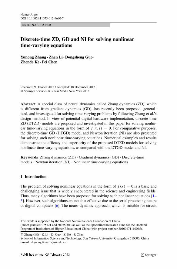
The above equation is actually equivalent to f (x(t), t) = (x(t)−sin(2.6t)−1)(x(t)−sin(2.6t) + 1) = 0, and its theoretical time-varying solutions x∗(t) are sin(2.6t) + 1and sin(2.6t) − 1, which are given here to verify the correctness of the iterativesolutions. The corresponding numerical results are shown in Figs. 1–4 and Tables 1and 2.

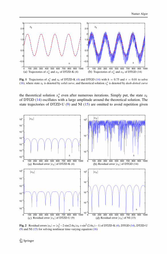
Specifically, Fig. 1 shows the states of DTZD-K (4) and DTGD (14) with step-sizeh = 0.75 and sampling gap τ = 0.01 for solving (16). To check the effectiveness ofsuch two solvers, the theoretical time-varying solution x∗

k = x∗(tk) = sin(2.6tk) +1 of (16) is shown, denoted by the dash-dotted curve in the figure. As shown inFig. 1a, the state xk of DTZD-K (4) converges to the theoretical solution x∗

k exactly.In contrast, the state xk generated by DTGD (14) [see Fig. 1b] does not fit well with

Numer Algor

0 100 200 300 400 500 600 700 800 900 1000−1

−0.5

0

0.5

1

1.5

2

2.5

3

0 100 200 300 400 500 600 700 800 900 1000−1

−0.5

0

0.5

1

1.5

2

2.5

3

(a) (b)

xk xk

Fig. 1 Trajectories of x∗k and xk of DTZD-K (4) and DTGD (14) with h = 0.75 and τ = 0.01 to solve

(16), where state xk is denoted by solid curve, and theoretical solution x∗k is denoted by dash-dotted curve

the theoretical solution x∗k even after numerous iterations. Simply put, the state xk

of DTGD (14) oscillates with a large amplitude around the theoretical solution. Thestate trajectories of DTZD-U (9) and NI (15) are omitted to avoid repetition given

0 100 200 300 400 500 600 700 800 900 1000

10−6

10−5

10−4

10−3

10−2

10−1

100

0 100 200 300 400 500 600 700 800 900 1000

10−2

10−1

100

0 100 200 300 400 500 600 700 800 900 1000

10−5

10−4

10−3

10−2

10−1

100

0 100 200 300 400 500 600 700 800 900 100010−4

10−3

10−2

10−1

100

(a) (b)

(c) (d)

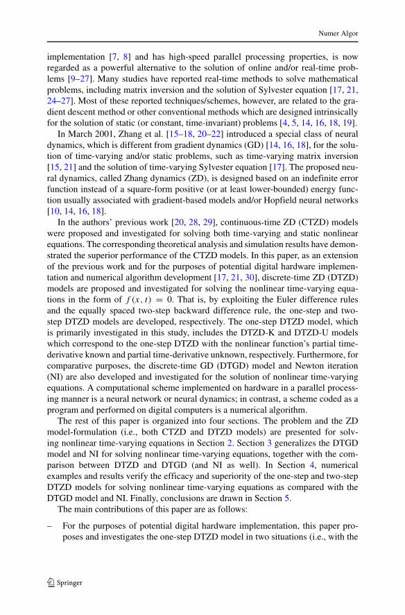
Fig. 2 Residual errors |ek | = |x2k −2 sin(2.6tk)xk+sin2(2.6tk)−1| of DTZD-K (4), DTGD (14), DTZD-U

(9) and NI (15) for solving nonlinear time-varying equation (16)

Numer Algor

10−3 10−2 10−110−6

10−5

10−4

10−3

10−2

10−1

100

101

τ

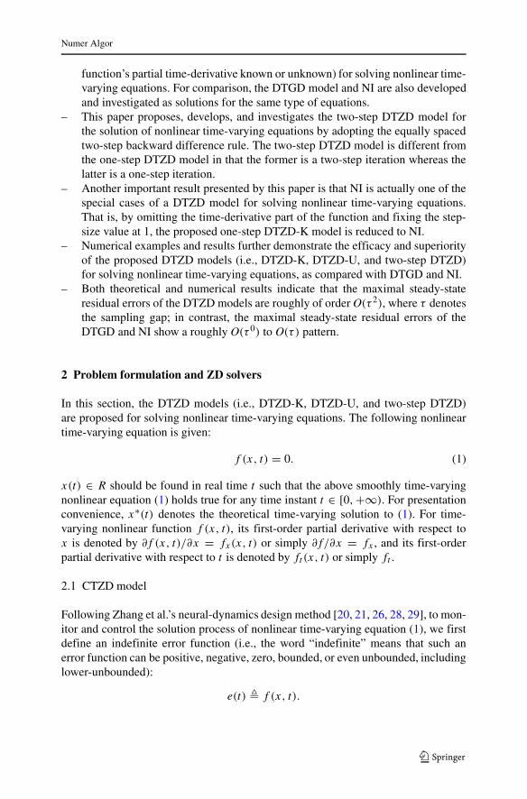
DTZD−KDTZD−UDTGDNI

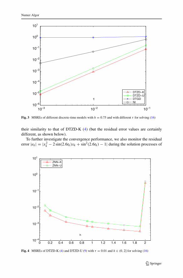
Fig. 3 MSREs of different discrete-time models with h = 0.75 and with different τ for solving (16)

their similarity to that of DTZD-K (4) (but the residual error values are certainlydifferent, as shown below).

To further investigate the convergence performance, we also monitor the residualerror |ek| = |x2

k − 2 sin(2.6tk)xk + sin2(2.6tk) − 1| during the solution processes of

0 0.2 0.4 0.6 0.8 1 1.2 1.4 1.6 1.8 210−4

10−3

10−2

10−1

100

101

h

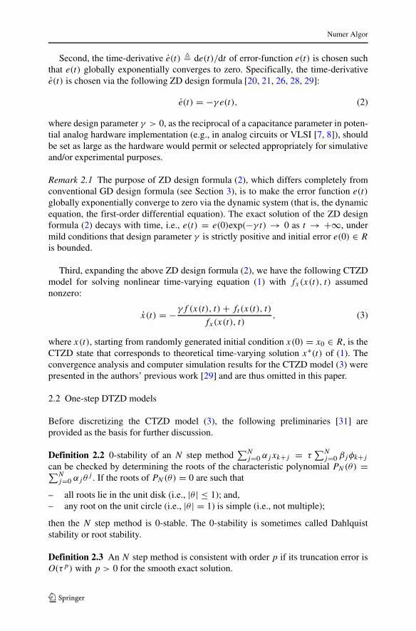
ZNN−KZNN−U

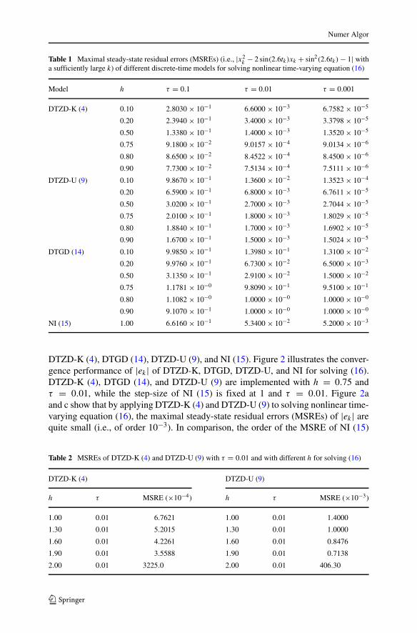
Fig. 4 MSREs of DTZD-K (4) and DTZD-U (9) with τ = 0.01 and h ∈ (0, 2] for solving (16)

Numer Algor

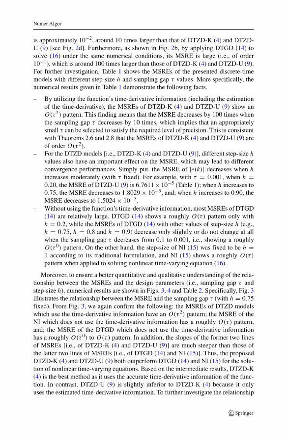
Table 1 Maximal steady-state residual errors (MSREs) (i.e., |x2k − 2 sin(2.6tk)xk + sin2(2.6tk) − 1| with

a sufficiently large k) of different discrete-time models for solving nonlinear time-varying equation (16)

Model h τ = 0.1 τ = 0.01 τ = 0.001

DTZD-K (4) 0.10 2.8030 × 10−1 6.6000 × 10−3 6.7582 × 10−5

0.20 2.3940 × 10−1 3.4000 × 10−3 3.3798 × 10−5

0.50 1.3380 × 10−1 1.4000 × 10−3 1.3520 × 10−5

0.75 9.1800 × 10−2 9.0157 × 10−4 9.0134 × 10−6

0.80 8.6500 × 10−2 8.4522 × 10−4 8.4500 × 10−6

0.90 7.7300 × 10−2 7.5134 × 10−4 7.5111 × 10−6

DTZD-U (9) 0.10 9.8670 × 10−1 1.3600 × 10−2 1.3523 × 10−4

0.20 6.5900 × 10−1 6.8000 × 10−3 6.7611 × 10−5

0.50 3.0200 × 10−1 2.7000 × 10−3 2.7044 × 10−5

0.75 2.0100 × 10−1 1.8000 × 10−3 1.8029 × 10−5

0.80 1.8840 × 10−1 1.7000 × 10−3 1.6902 × 10−5

0.90 1.6700 × 10−1 1.5000 × 10−3 1.5024 × 10−5

DTGD (14) 0.10 9.9850 × 10−1 1.3980 × 10−1 1.3100 × 10−2

0.20 9.9760 × 10−1 6.7300 × 10−2 6.5000 × 10−3

0.50 3.1350 × 10−1 2.9100 × 10−2 1.5000 × 10−2

0.75 1.1781 × 10−0 9.8090 × 10−1 9.5100 × 10−1

0.80 1.1082 × 10−0 1.0000 × 10−0 1.0000 × 10−0

0.90 9.1070 × 10−1 1.0000 × 10−0 1.0000 × 10−0

NI (15) 1.00 6.6160 × 10−1 5.3400 × 10−2 5.2000 × 10−3

DTZD-K (4), DTGD (14), DTZD-U (9), and NI (15). Figure 2 illustrates the conver-gence performance of |ek| of DTZD-K, DTGD, DTZD-U, and NI for solving (16).DTZD-K (4), DTGD (14), and DTZD-U (9) are implemented with h = 0.75 andτ = 0.01, while the step-size of NI (15) is fixed at 1 and τ = 0.01. Figure 2aand c show that by applying DTZD-K (4) and DTZD-U (9) to solving nonlinear time-varying equation (16), the maximal steady-state residual errors (MSREs) of |ek| arequite small (i.e., of order 10−3). In comparison, the order of the MSRE of NI (15)

Table 2 MSREs of DTZD-K (4) and DTZD-U (9) with τ = 0.01 and with different h for solving (16)

DTZD-K (4) DTZD-U (9)

h τ MSRE (×10−4) h τ MSRE (×10−3)

1.00 0.01 6.7621 1.00 0.01 1.4000

1.30 0.01 5.2015 1.30 0.01 1.0000

1.60 0.01 4.2261 1.60 0.01 0.8476

1.90 0.01 3.5588 1.90 0.01 0.7138

2.00 0.01 3225.0 2.00 0.01 406.30

Numer Algor

is approximately 10−2, around 10 times larger than that of DTZD-K (4) and DTZD-U (9) [see Fig. 2d]. Furthermore, as shown in Fig. 2b, by applying DTGD (14) tosolve (16) under the same numerical conditions, its MSRE is large (i.e., of order10−1), which is around 100 times larger than those of DTZD-K (4) and DTZD-U (9).For further investigation, Table 1 shows the MSREs of the presented discrete-timemodels with different step-size h and sampling gap τ values. More specifically, thenumerical results given in Table 1 demonstrate the following facts.

– By utilizing the function’s time-derivative information (including the estimationof the time-derivative), the MSREs of DTZD-K (4) and DTZD-U (9) show anO(τ 2) pattern. This finding means that the MSRE decreases by 100 times whenthe sampling gap τ decreases by 10 times, which implies that an appropriatelysmall τ can be selected to satisfy the required level of precision. This is consistentwith Theorems 2.6 and 2.8 that the MSREs of DTZD-K (4) and DTZD-U (9) areof order O(τ 2).

– For the DTZD models [i.e., DTZD-K (4) and DTZD-U (9)], different step-size h

values also have an important effect on the MSRE, which may lead to differentconvergence performances. Simply put, the MSRE of |e(k)| decreases when h

increases moderately (with τ fixed). For example, with τ = 0.001, when h =0.20, the MSRE of DTZD-U (9) is 6.7611 ×10−5 (Table 1); when h increases to0.75, the MSRE decreases to 1.8029 × 10−5, and; when h increases to 0.90, theMSRE decreases to 1.5024 × 10−5.

– Without using the function’s time-derivative information, most MSREs of DTGD(14) are relatively large. DTGD (14) shows a roughly O(τ) pattern only withh = 0.2, while the MSREs of DTGD (14) with other values of step-size h (e.g.,h = 0.75, h = 0.8 and h = 0.9) decrease only slightly or do not change at allwhen the sampling gap τ decreases from 0.1 to 0.001, i.e., showing a roughlyO(τ 0) pattern. On the other hand, the step-size of NI (15) was fixed to be h =1 according to its traditional formulation, and NI (15) shows a roughly O(τ)

pattern when applied to solving nonlinear time-varying equation (16).

Moreover, to ensure a better quantitative and qualitative understanding of the rela-tionship between the MSREs and the design parameters (i.e., sampling gap τ andstep-size h), numerical results are shown in Figs. 3, 4 and Table 2. Specifically, Fig. 3illustrates the relationship between the MSRE and the sampling gap τ (with h = 0.75fixed). From Fig. 3, we again confirm the following: the MSREs of DTZD modelswhich use the time-derivative information have an O(τ 2) pattern; the MSRE of theNI which does not use the time-derivative information has a roughly O(τ) pattern,and; the MSRE of the DTGD which does not use the time-derivative informationhas a roughly O(τ 0) to O(τ) pattern. In addition, the slopes of the former two linesof MSREs [i.e., of DTZD-K (4) and DTZD-U (9)] are much steeper than those ofthe latter two lines of MSREs [i.e., of DTGD (14) and NI (15)]. Thus, the proposedDTZD-K (4) and DTZD-U (9) both outperform DTGD (14) and NI (15) for the solu-tion of nonlinear time-varying equations. Based on the intermediate results, DTZD-K(4) is the best method as it uses the accurate time-derivative information of the func-tion. In contrast, DTZD-U (9) is slightly inferior to DTZD-K (4) because it onlyuses the estimated time-derivative information. To further investigate the relationship

Numer Algor

between the MSREs of the DTZD models and the step-size h, Fig. 4 and Table 2illustrate the numerical results synthesized by DTZD-K (4) and DTZD-U (9) withdifferent step-size h values and sampling gap τ = 0.01. In addition to Table 1, Fig. 4and Table 2 further confirm the theoretical results of Theorem 2.9 that superior per-formance can be achieved with step-size h ∈ (0, 2), which ensures the effectivenessof the proposed DTZD models for solving nonlinear time-varying equations [e.g.,(16)]. In other words, the MSRE is affected by the different values of h.

Example 4.2 As illustrated in the previous example, DTZD-U model (9) is effectivein solving nonlinear time-varying equations. For further investigation, another non-linear time-varying equation with ft (x(t), t) unknown (or more difficult to obtain) isconsidered:

f (x(t), t) = x3(t) − (sin(cos(cos(1.2t))) + 2)x2(t)

+ x(t) − sin(cos(cos(1.2t))) − 2 = 0. (17)

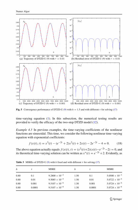
The above equation equals f (x(t), t) = (x2(t) + 1)(x(t) − sin(cos(cos(1.2t))) −2) = 0, and its theoretical time-varying solution is x∗(t) = sin(cos(cos(1.2t))) +2. Evidently, DTZD-K (4) may not be suitable for the solution of such a nonlinearequation because it is much more difficult to obtain ft (x(t), t) analytically in thisexample [in other words, ft (x(t), t) is assumed in this case to be unknown]. Thus,using DTZD-U (9) to solve (17) is preferable. The corresponding numerical resultsare shown in Fig. 5 and Table 3.

Specifically, as shown in Fig. 5a and c, the states of DTZD-U model (9) with h =1.5 and with different values of sampling gap τ (i.e., τ = 0.01 and τ = 0.001) bothconverge to the theoretical time-varying solution very well. In addition, Fig. 5b andd show that the MSREs of DTZD-U model (9) are quite small, which demonstratesthe efficacy of the DTZD-U model (9) in solving nonlinear time-varying equation(17) with ft (x(t), t) unknown. Furthermore, the numerical results shown in Table 3illustrate and confirm that the MSRE of DTZD-U model (9) decreases in an O(τ 2)

pattern as the sampling gap τ decreases. Thus, Theorem 2.8 about the error of DTZD-U model (9) being of order O(τ 2) is again substantiated, which implies that DTZD-Umodel (9) is effective in solving nonlinear time-varying equations.

In summary, the above numerical results (i.e., Figs. 1–5 and Tables 1–3) demon-strate the efficacy and superiority of both the DTZD-K model (4) and DTZD-U (9)models in solving nonlinear time-varying equations whether ft (x(t), t) is known ornot, as compared with the DTGD model (14) and NI (15). The above remarks supportTheorems 2.4 through 2.9.

4.2 Two-step DTZD for solving nonlinear time-varying equation

As mentioned previously, the CTZD model (3) can be discretized by using theequally spaced two-step backward difference rule, and thus its discrete-time model[i.e., two-step DTZD model (12)] is generalized and developed for solving nonlinear

Numer Algor

0 100 200 300 400 500 600 700 800 900 10002.4

2.45

2.5

2.55

2.6

2.65

2.7

2.75

2.8

2.85

0 100 200 300 400 500 600 700 800 900 1000

10−6

10−5

10−4

10−3

10−2

10−1

100

0 1000 2000 3000 4000 5000 6000 7000 8000 9000 100002.4

2.45

2.5

2.55

2.6

2.65

2.7

2.75

2.8

2.85

0 1000 2000 3000 4000 5000 6000 7000 8000 9000 10000

10−8

10−6

10−4

10−2

100

(c) (d)

(a) (b)

x

x

Fig. 5 Convergence performance of DTZD-U (9) with h = 1.5 and with different τ for solving (17)

time-varying equation (1). In this subsection, the numerical testing results areprovided to verify the efficacy of the two-step DTZD model (12).

Example 4.3 In previous examples, the time-varying coefficients of the nonlinearfunctions are sinusoidal. This time, we consider the following nonlinear time-varyingequation with exponential coefficients:

f (x(t), t) = x3(t) − (e−2t + 2)x2(t) + 2x(t) − 2e−2t − 4 = 0. (18)

The above equation actually equals f (x(t), t) = (x2(t)+2)(x(t)−e−2t −2) = 0, andits theoretical time-varying solution can be written as x∗(t) = e−2t +2. Evidently, as

Table 3 MSREs of DTZD-U (9) with h fixed and with different τ for solving (17)

h τ MSRE h τ MSRE

0.80 0.1 9.2800 × 10−2 1.50 0.1 5.0500 × 10−2

0.80 0.01 9.5085 × 10−4 1.50 0.01 5.0722 × 10−4

0.80 0.001 9.5107 × 10−6 1.50 0.001 5.0724 × 10−6

0.80 0.0001 9.5107 × 10−8 1.50 0.0001 5.0724 × 10−8

Numer Algor

t tends to +∞ (that is, t is large enough), time-varying nonlinear equation (18) tendsto f (x) = x3 − 2x2 + 2x − 4 = 0 (i.e., a static nonlinear equation) and x∗(t) tendsto 2 (i.e., a static root).

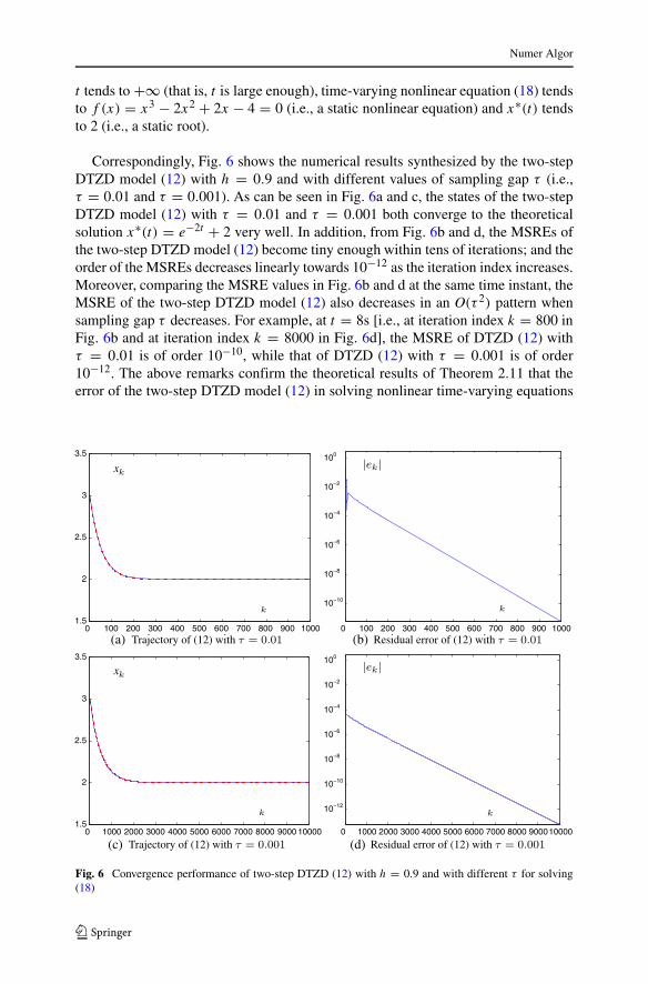
Correspondingly, Fig. 6 shows the numerical results synthesized by the two-stepDTZD model (12) with h = 0.9 and with different values of sampling gap τ (i.e.,τ = 0.01 and τ = 0.001). As can be seen in Fig. 6a and c, the states of the two-stepDTZD model (12) with τ = 0.01 and τ = 0.001 both converge to the theoreticalsolution x∗(t) = e−2t + 2 very well. In addition, from Fig. 6b and d, the MSREs ofthe two-step DTZD model (12) become tiny enough within tens of iterations; and theorder of the MSREs decreases linearly towards 10−12 as the iteration index increases.Moreover, comparing the MSRE values in Fig. 6b and d at the same time instant, theMSRE of the two-step DTZD model (12) also decreases in an O(τ 2) pattern whensampling gap τ decreases. For example, at t = 8s [i.e., at iteration index k = 800 inFig. 6b and at iteration index k = 8000 in Fig. 6d], the MSRE of DTZD (12) withτ = 0.01 is of order 10−10, while that of DTZD (12) with τ = 0.001 is of order10−12. The above remarks confirm the theoretical results of Theorem 2.11 that theerror of the two-step DTZD model (12) in solving nonlinear time-varying equations

0 100 200 300 400 500 600 700 800 900 10001.5

2

2.5

3

3.5

0 100 200 300 400 500 600 700 800 900 1000

10−10

10−8

10−6

10−4

10−2

100

0 1000 2000 3000 4000 5000 6000 7000 8000 9000 100001.5

2

2.5

3

3.5

0 1000 2000 3000 4000 5000 6000 7000 8000 900010000

10−12

10−10

10−8

10−6

10−4

10−2

100

(a) (b)

(c) (d)

x

x

Fig. 6 Convergence performance of two-step DTZD (12) with h = 0.9 and with different τ for solving(18)

Numer Algor

[e.g., (18)] is of O(τ 2) pattern. The efficacy of the two-step DTZD model (12) insolving nonlinear time-varying equations is thus demonstrated.

5 Conclusions

Following Zhang et al.’s design method, we revisited a special class of neuraldynamics (i.e., CTZD) for solving nonlinear time-varying equations. For purposes ofpotential application on digital circuits or computers, three types of DTZD models,namely, DTZD-K (4), DTZD-U (9), and two-step DTZD (12), were proposed, ana-lyzed, and investigated in this paper for solving nonlinear time-varying equations.The different values of sampling gap τ and step-size h significantly affect the errors(e.g., the MSREs) of the proposed DTZD models. Moreover, the numerical testingresults confirmed that the proposed DTZD models have much better convergence per-formance due to their utilization of the time-derivative information, as compared withthe DTGD model (14) and NI (15) which do not use the time-derivative information.

Acknowledgments The authors sincerely thank the editor and reviewers for their constructive andinspiring comments which greatly helped improve the presentation and the quality of the paper.

References

1. Ujevic, N.: A method for solving nonlinear equations. Appl. Math. Comput. 174, 1416–1426 (2006)2. Sharma, J.R.: A composite third order Newton-steffensen method for solving nonlinear equations.

Appl. Math. Comput. 169, 242–246 (2005)3. Chun, C.: Construction of Newton-like iteration methods for solving nonlinear equations. Numer.

Math. 104, 297–315 (2006)4. Frontini, M.: Hermite interpolation and a new iterative method for the computation of the roots of

non-linear equations. Calcolo 40, 109–119 (2003)5. Zhang, Y., Xiao, L., Ruan, G., Li, Z.: Continuous and discrete time Zhang dynamics for time-varying

4th root finding. Numer. Algor. 57, 35–51 (2011)6. Zhang, Y., Leithead, W.E., Leith, D.J.: Time-series Gaussian process regression based on Toeplitz

computation of O(N2) operations and O(N)-level storage. In: Proceedings of the 44th IEEEConference on Decision and Control, pp. 3711–3716 (2005)

7. Mead, C.: Analog VLSI and Neural Systems. Addison-Wesley, Reading, MA (1989)8. Zhang, Y., Ma, W., Li, K., Yi, C.: Brief history and prospect of coprocessors. China Sci. Tech. Inf. 13,

115–117 (2008)9. Zhang, Y., Xu, D.: Global dynamics for non-autonomous reaction-diffusion neural networks with

time-varying delays. Theor. Comput. Sci. 403, 3–10 (2008)10. Lenze, B.: Linking discrete orthogonality with dilation and translation for incomplete sigma-pi neural

networks of Hopfield-type. Discrete Appl. Math. 89, 169–180 (1998)11. Wang, J.: A recurrent neural network for real-time matrix inversion. Appl. Math. Comput. 55, 89–100

(1993)12. Ganesh, M., Mustapha, K.: A fully discrete H 1-Galerkin method with quadrature for nonlinear

advection-diffusion-reaction equations. Numer. Algor. 43, 355–383 (2003)13. Shi, Y.: A globalization procedure for solving nonlinear systems of equations. Numer. Algor. 12, 273–

286 (2003)14. Mohamad, S., Gopalsamy, K.: Dynamics of a class of discrete-time neural networks and their

continuous-time counterparts. Math. Comput. Simul. 53, 1–39 (2000)15. Zhang, Y., Ma, W., Cai, B.: From Zhang neural network to Newton iteration for matrix inversion.

IEEE Trans. Circuits Syst. 56, 1405–1415 (2009)

Numer Algor

16. Zhang, Y., Yang, Y.: Simulation and comparison of Zhang neural network and gradient neural networksolving for time-varying matrix square roots. In: Proceedings of the 2nd International Symposium onIntelligent Information Technology Application, pp. 966–970 (2008)

17. Zhang, Y., Jiang, D., Wang, J.: A recurrent neural network for solving Sylvester equation with time-varying coefficients. IEEE Trans. Neural Netw. 13, 1053–1063 (2002)

18. Zhang, Y., Li, Z.: Zhang neural network for online solution of time-varying convex quadratic programsubject to time-varying linear-equality constraints. Phys. Lett. A 373, 1639–1643 (2009)

19. Brezinski, C.: A classification of quasi-Newton methods. Numer. Algor. 33, 123–135 (2003)20. Zhang, Y., Xu, P., Tan, N.: Solution of nonlinear equations by continuous-time and discrete-time

Zhang dynamics and more importantly their links to Newton iteration. In: Proceedings of IEEEInternational Conference on Information, Communications and Signal Processing, pp. 1–5 (2009)

21. Zhang, Y., Ge, S.: Design and analysis of a general recurrent neural network model for time-varyingmatrix inversion. IEEE Trans. Neural Netw. 16, 1477–1490 (2005)

22. Zhang, Y.: A set of nonlinear equations and inequalities arising in robotics and its online solution viaa primal neural network. Neurocomputing 70, 513–524 (2006)

23. The MathWorks, Inc.: Simulink 7 Getting Started Guide. Natick, MA (2008)24. Guo, B., Wang, D., Shen, Y., Li, Z.: A Hopfield neural network approach for power optimization of

real-time operating systems. Neural Comput. Appl. 17, 11–17 (2008)25. Wu, A., Tam, P.K.S.: A neural network methodology and strategy of quadratic optimization. Neural

Comput. Appl. 8, 283–289 (1999)26. Zhang, Y., Chen, Z., Chen, K., Cai, B.: Zhang neural network without using time-derivative informa-

tion for constant and time-varying matrix inversion. In: Proceedings of International Joint Conferenceon Neural Networks, pp. 142–146 (2008)

27. Steriti, R.J., Fiddy, M.A.: Regularized image reconstruction using SVD and a neural network methodfor matrix inversion. IEEE Trans. Signal Process. 41, 3074–3077 (1993)

28. Zhang, Y., Xu, P., Tan, N.: Further studies on Zhang neural-dynamics and gradient dynamics for onlinenonlinear equations Solving. In: Proceedings of the IEEE International Conference on Automationand Logistics, pp. 566–571 (2009)

29. Zhang, Y., Yi, C., Guo, D., Zheng, J.: Comparison on Zhang neural dynamics and gradient-basedneural dynamics for online solution of nonlinear time-varying equations. Neural Comput. Appl. 20,1–7 (2010)

30. Perez-IIzarbe, M.J.: Convergence analysis of a discrete-time recurrent neural network to performquadratic real optimization with bound constraints. IEEE Trans. Neural Netw. 9, 1344–1351 (1998)

31. David, F.G., Desmond, J.H.: Numerical Methods for Ordinary Differential Equations: Initial ValueProblems. Springer, England (2010)

32. Mathews, J.H., Fink, K.D.: Numerical Methods Using MATLAB. Publishing House of ElectronicsIndustry, Beijing (2005)

33. Zhang, Y., Guo, D., Xu, S., Li, H.: Verification and practice on first-order numerical differentiationformulas for unknown target functions. J. Gansu. Sci. 21, 13–18 (2009)

34. Mitra, S.K.: Digital Signal Processing: A Computrer-Based Approach. Tsinghua University Press,Beijing (2006)