Discrete-Time Signal Processing and Makhoul’s

Conjecture

Michael Rabbat

rabbat@cae.wisc.edu

ECE/Math 842 Project Report, Fall 2004

Abstract

This report surveys the role that polynomials and algebra play in investigating some fundamental

properties of all-pass signals and systems. All-pass systems are an important concept in the theory of

discrete-time signal processing. In particular, we summarize work regarding Makhoul’s conjecture on the

locations of peaks in the impulse response of an all-pass system (also called an all-pass signal).

1 Discrete-Time Systems and Signals

Generally speaking, the field of discrete-time signal processing is focused on studying systems which take

as input a sequence {xn} and generate an output sequence {yn}. Linear time-invariant systems can be

described using a recurrence relation between the input and output sequences of the form

yn + a1yn−1 + · · ·+ apya−p = b0xn + b1xn−1 + · · ·+ bqxn−q, (1)

where, for most practical purposes, the aj and bj are real-valued coefficients. Systems with complex co-

efficients are sometimes studied, but throughout this paper we will focus on the systems with real-valued

coefficients. We generally think of n as indexing time, and we say that the relation above corresponds to a

causal linear time-invariant system since output yt only depends on input and output values for times n ≤ t.

Conceptually, let z−1 represent a unit delay. The z-transform of a sequence {wn} is defined as

W (z) =∞∑

n=−∞wnz−n. (2)

Rewriting the recurrence relation in terms of the z-transforms of xn and yn yields

Y (z)(1 + a1z−1 + · · ·+ apz

−p) = X(z)(b0 + b1z−1 + · · ·+ bqz

−q),

1

or equivalently,

Y (z) = H(z)X(z),

where

H(z) =b0 + b1z

−1 + · · ·+ bqz−q

1 + a1z−1 + · · ·+ apz−p=

B(z)A(z)

(3)

is called the transfer function of the system or filter. The z-transform representation is useful in a number

of different ways. For instance, the (complex-valued) roots of the polynomial zqA(z) are called the poles of

the system, and the system is said to be stable if all its poles lie within the complex unit circle. Evaluating

the transfer function at z = ejω yields the frequency response of the system,

H(ω) =∑q

k=0 bke−jkω

1 +∑p

k=1 ake−jkω.

2 All-Pass Systems and Signals

An all-pass system is a specific type of causal linear time-invariant system named so because it has unitary

magnitude response; i.e., |H(ω)| = 1 for −π ≤ ω ≤ π; i.e., it passes all frequencies unattenuated. The most

general z-transform representation of a causal all-pass system with real-valued impulse response is a product

of factors with complex poles being paired with their complex conjugates [5]:

H(z) =R∏

k=1

z−1 − rk

1− rkz−1

C∏k=1

(z−1 − c∗k)(z−1 − ck)(1− ckz−1)(1− c∗kz−1)

,

where rk’s are real poles, and ck’s are complex poles. The given form corresponds to an order-p all-pass

system where p = R + 2C. Expanding the products yields the rational transfer function

H(z) =a1 + a2z

−1 + · · ·+ z−p

1 + ap−1z−1 + · · ·+ a1z−p,

where the numerator and denominator are reciprocal polynomials in z−1 with real-valued coefficients ak.

The impulse response of a causal linear time-invariant system, denoted hn, is the output sequence corre-

sponding to the input xn = δn where

δn =

1 if n=0,

0 otherwise.(4)

The impulse response of an order-p all-pass system is sometimes called an order-p all-pass sequence (or

signal).

2

3 Makhoul’s Conjecture

In 1986 John Makhoul published Problem 86-12, “Conjectured Location of Maximum Amplitude in an

All-Pass Sequence” in the SIAM Review [2]. Makhoul conjectured the following.

Conjecture 1 (Makhoul ‘86, [2]) Let hn be an all-pass sequence and define the peak location to be n∗

such that |hn∗ | = maxn|hn| and |hn| < |hn∗ | for all n > n∗. Prove (or disprove) that n∗ ∈ [0, 2p− 1].

In this original article Makhoul verified the conjecture for p = 1. In 1991 Makhoul published a followup

paper with Allan Steinhardt which contained results pertaining to the locations of peak values of general

causal signals (not necessarily all-pass). The conjecture was restated within the body of this article.

Fourteen years after the original announcement (with no further progress having been made), Makhoul

made another appeal to the community. This time an article was published in IEEE Signal Processing

Magazine announcing the Makhoul Conjecture Challenge, offering a prize of US$1000 to anyone who could

prove or disprove the conjecture [3]. At IEEE ICASSP the following year, Makhoul’s conjecture was verified

for p = 2 by Nigel Boston [1]. At the same conference, counterexamples were reported by Ram Rajagopal

and Lothar Wenzel for p = 6 and higher [7]. In fact, based on examples due to A. Moriat and J. Gerved, it

appears that the peak location can be made arbitrarily large for sufficiently large p (an example is given in

[7] for which n∗ > 5p with p = 4000). Thus, Makhoul’s conjecture does not hold in general. However, the

“right” bound on the peak location for an order-p causal all-pass sequence still remains unknown.

4 Applications of All-Pass Filters

Before proceeding with a more in-depth look at the algebra behind Makhoul’s conjecture we survey some

applications using all-pass filters to motivate the study of their fundamental properties.

4.1 System Testing and Identification

Makhoul’s work on all-pass filters was originally motivated by applications in the testing of digital systems

[2]. The impulse response of a digital filter is defined as the output of the system when the input is an impulse,

δn, as defined in (4). This has the effect of exciting all frequencies, so that the impulse response, hn, in some

sense contains a “frequency signature” for the filter or system. In [6], Rabiner and Crochiere suggest that,

practically speaking, using impulse may be unnecessarily for determining the frequency response of a system

or for testing the system by exciting the entire frequency spectrum. Instead, they propose using an all-pass

sequence which will equivalently excite all frequencies.

3

4.2 Frequency-Response Compensation

Ensuring that systems have linear phase response (i.e., ∠H(ω)) over bands of passed frequency is important

topic in discrete-time filter design [5]. As an illustration of why linear phase is important, consider the

ideal delay system with impulse response hdelayn = δn−nd

. Thus, the output of the system is identical

to the input, delayed by nd units of time (e.g., yn+nd= xn). The frequency response of this system is

Hdelay(ω) = e−jωnd , so the system has a phase response ∠Hdelay(ω) = −ωnd which is a linear function

of ω. Systems with nonlinear phase have the effect of distorting their input which is undesirable in many

applications (e.g., audio processing).

Recall that a system H(z) is stable if all of its poles (roots of the denominator polynomial in (3)) lie

in the unit circle. We refer to H(z) as a minimum-phase system if all of its poles and zeros lie in the unit

circle. The name minimum-phase comes from the following three interesting properties. Let Hmin(z) be

a minimum-phase system and let H be the collection of all stable causal systems with magnitude response

equivalent to |Hmin(ω)|.

1. Of all H ∈ H, Hmin has the minimum phase-lag, max∠H(ω).

2. Of all H ∈ H, Hmin has the minimum group-delay (minimum deviation from linearity).

3. Of all H ∈ H, Hmin has the minimum energy-delay (most of its energy is concentrated around n = 0).

Note that the inverse of a minimum-phase system is also stable.

An important but straightforward result is that any system function of the form (3) can be factored

according to,

H(z) = Hmin(z)Hap(z),

where Hmin(z) is a minimum-phase system and Hap(z) is an all-pass system. Thus, if we are given spec-

ifications for a system with frequency response Hspec(z) which is not minimum-phase, one might consider

designing a compensating filter, Hc(z), so that the concatenation of the two filters, G(z) = Hspec(z)Hc(z),

is a minimum-phase system. Based on the minimum-phase/all-pass decomposition above, this filter would

be the inverse of an all-pass filter. However we know that stable all-pass filters have poles in the unit circle

and zeros outside the unit circle (since the numerator of an all-pass filter is the reciprocal polynomial of

the denominator). Alternatively, we design a filter H ′(z) with frequency response equivalent to H(z) by

reflecting the zeros of H(z) which lie outside the unit circle to their conjugate reciprocal locations inside the

unit circle [5].

4

5 The Case of p = 1

Verifying Makhoul’s claim for p = 1 is relatively straightforward [2]. A first-order all-pass system has a single

real-valued pole, α, with |α| < 1. Its transfer function is given by

H(z) =α + z−1

1 + αz−1,

and the equivalent recurrence relation is

yn + αyn−1 = αxn + xn−1.

The values of the impulse response are given by

h0 = α,

h1 = 1− α2,

h2 = −(α3 − α),...

hn = (−1)ngn(α), for n ≥ 1,

where

gn(α) = αn+1 − αn−1. (5)

For n ≥ 1 we have

|hn| = |αn+1 − αn−1|

= (|α|)n|α− 1|

< |h1|,

since |α| < 1. Thus the peak either occurs for n = 0 or n = 1 and the conjecture is verified.

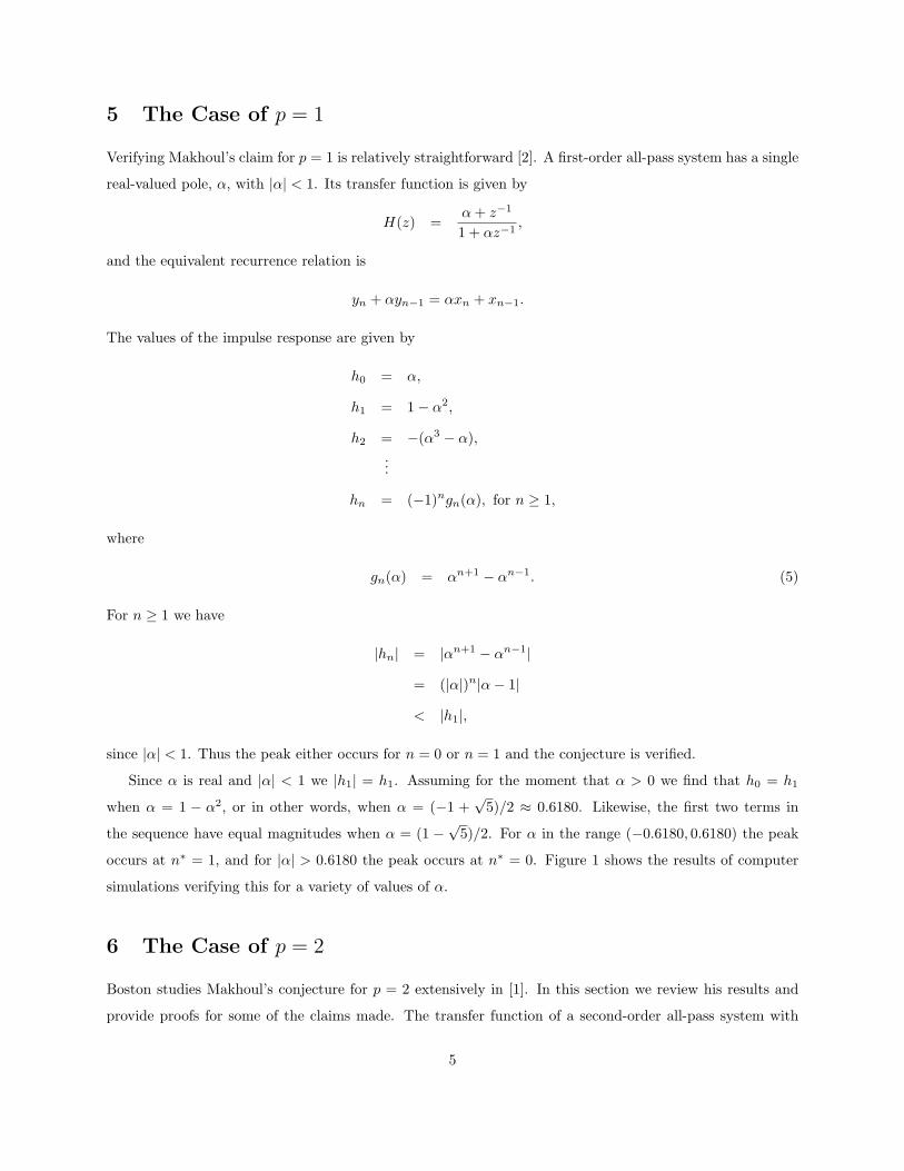
Since α is real and |α| < 1 we |h1| = h1. Assuming for the moment that α > 0 we find that h0 = h1

when α = 1 − α2, or in other words, when α = (−1 +√

5)/2 ≈ 0.6180. Likewise, the first two terms in

the sequence have equal magnitudes when α = (1 −√

5)/2. For α in the range (−0.6180, 0.6180) the peak

occurs at n∗ = 1, and for |α| > 0.6180 the peak occurs at n∗ = 0. Figure 1 shows the results of computer

simulations verifying this for a variety of values of α.

6 The Case of p = 2

Boston studies Makhoul’s conjecture for p = 2 extensively in [1]. In this section we review his results and

provide proofs for some of the claims made. The transfer function of a second-order all-pass system with

5

−1 −0.8 −0.6 −0.4 −0.2 0 0.2 0.4 0.6 0.8 10

0.1

0.2

0.3

0.4

0.5

0.6

0.7

0.8

0.9

1

alpha

peak

loca

tion

Figure 1: Peak locations for an order-1 all-pass signal.

poles α and β is

H(z) =(α− z−1)(β − z−1)

(1− αz−1)(1− βz−1)

=a + bz−1 + z−2

1 + bz−1 + az−2,

where a = αβ and b = −α− β. The corresponding recurrence relation is

yn + byn−1 + ayn−2 = axn + bxn−1 + xn−2,

and the first few values of the impulse response are

h0 = a,

h1 = b− ab,

h2 = 1− a2 − b2 + ab2.

In order to determine the peak location it is useful to first establish a general expression for the impulse

response values in terms of α and β.

Lemma 1 (Boston ‘00, [1]) Let hn be an order-p all-pass impulse response with h0 = αβ. Then for n ≥ 1

hn =

(gn(α)− gn(β)

)αβ − 1α− β

if α 6= β,

g′n(α)(α2 − 1

)if α = β,

where gn(x) is as defined in (5) and g′n(x) = (n + 1)xn − (n− 1)xn−2.

6

Proof: We provide a proof using induction. To establish the induction base, first consider α 6= β:

h1 = b− ab

= (−α− β)− αβ(−α− β)

= (α + β)(αβ − 1)

= (α2 − β2)αβ − 1α− β

=((α2 − 1)− (β2 − 1)

)αβ − 1α− β

,

and

h2 = 1− a2 − b2 + ab2

= 1− (αβ)2 − (−α− β)2 + αβ(−α− β)2

= (αβ − 1)[(α + β)2 − (1 + αβ)

]= (α− β)(α2 + αβ + β2 − 1)

αβ − 1α− β

=((α3 − α)− (β3 − β)

)αβ − 1α− β

.

Similar manipulations yield the corresponding expressions for the case α = β. To verify the induction step

for distinct α and β we only need to check that

−(−α− β)(gn−1(α)− gn−1(β)

)− αβ

(gn−2(α)− gn−2(β)

)= (α + β)

(αn − αn−2 − βn + βn−2

)− αβ

(αn−1 − αn−3 − βn−1 + βn−3

)= αn+1 − αn−1 − βn+1 + βn−1

= gn(α)− gn(β).

Likewise, for α = β, we confirm that

−(−2α)g′n−1(α)− α2g′n−2(α) = 2α(nαn−1 − (n− 2)αn−3

)− α2

((n− 1)αn−2 − (n− 3)αn−4

)=

(2n− (n− 1)

)αn +

(− 2(n− 2) + (n− 3)

)αn−2

= (n + 1)αn − (n− 1)αn−2

= g′n(α).

Next we use this nice representation to verify Makhoul’s conjecture for p = 2. There are two general

situations to consider for the roots of a stable real causal all-pass system. Either both roots are real-valued,

or they are complex conjugates.

7

−1 −0.8 −0.6 −0.4 −0.2 0 0.2 0.4 0.6 0.8 1−1

−0.8

−0.6

−0.4

−0.2

0

0.2

0.4

0.6

0.8

1

α

β

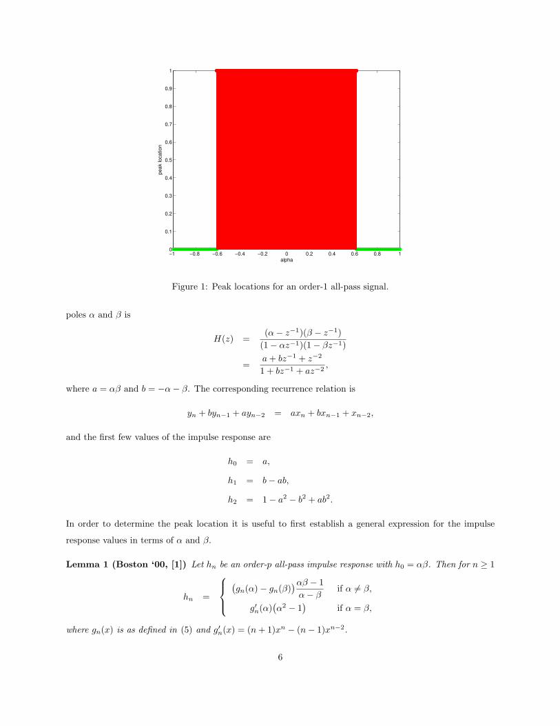
Figure 2: Peak locations of a stable causal all-pass sequence when the poles of the corresponding system,

α and β, are real-valued. The green, red, and blue regions correspond to pole values for which the peak

location occurs at n∗ = 0, 1, and 2 respectively.

6.1 Real Roots

Figure 2 depicts the results of computationally exploring various real-valued choices for the poles α and β.

The green, red, and blue regions correspond to choices of (α, β) for which the peak location is n∗ = 0, 1,

and 2 respectively. To rigorously verify that there is no real-valued choice of (α, β) ∈ (−1, 1)2 resulting in

an all-pass sequence with peak value beyond n = 2, Boston considers four distinct cases [1]. In each case,

we would like to show that |hn| < max{|h0|, |h1|, |h2|} for all n ≥ 3 and α ∈ (−1, 1).

Case I (α = β): Observe that if α < 0 we can write

|g′n(α)| =∣∣(n + 1)αn − (n− 1)αn−2

∣∣=

∣∣(−1)n((n + 1)(−α)n − (n− 1)(−α)n−2

)∣∣,and the factor (−1)n does not affect the magnitude. So without loss of generality assume α > 0.

Makhoul’s conjecture is verified by noting that for n ≥ 3 the function

g′1(α)− g′n(α) = 2α− (n + 1)αn + (n− 1)αn−2 (6)

is bounded below by 2α if α < 0.5, and bounded below by g′1(α) − g′3(α) > 0 for α ≥ 0.5. Thus it is

always positive, and for all n ≥ 3, |h1| > |hn| verifying the conjecture in this case.

8

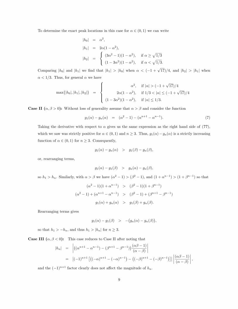
To determine the exact peak locations in this case for α ∈ (0, 1) we can write

|h0| = α2,

|h1| = 2α(1− α2),

|h2| =

(3α2 − 1)(1− α2), if α ≥√

1/3

(1− 3α2)(1− α2), if α <√

1/3.

Comparing |h0| and |h1| we find that |h1| > |h0| when α < (−1 +√

17)/4, and |h2| > |h1| when

α < 1/3. Thus, for general α we have

max{|h0|, |h1|, |h2|} =

α2, if |α| > (−1 +

√17)/4

2α(1− α2), if 1/3 < |α| ≤ (−1 +√

17)/4

(1− 3α2)(1− α2), if |α| ≤ 1/3.

Case II (α, β > 0): Without loss of generality assume that α > β and consider the function

g1(α)− gn(α) = (α2 − 1)− (αn+1 − αn−1). (7)

Taking the derivative with respect to α gives us the same expression as the right hand side of (??),

which we saw was strictly positive for α ∈ (0, 1) and n ≥ 3. Thus, g1(α)− gn(α) is a strictly increasing

function of α ∈ (0, 1) for n ≥ 3. Consequently,

g1(α)− gn(α) > g1(β)− gn(β),

or, rearranging terms,

g1(α)− g1(β) > gn(α)− gn(β),

so h1 > hn. Similarly, with α > β we have (α2 − 1) > (β2 − 1), and (1 + αn−1) > (1 + βn−1) so that

(α2 − 1)(1 + αn−1) > (β2 − 1)(1 + βn−1)

(α2 − 1) + (αn+1 − αn−1) > (β2 − 1) + (βn+1 − βn−1)

g1(α) + gn(α) > g1(β) + gn(β).

Rearranging terms gives

g1(α)− g1(β) > −(gn(α)− gn(β)

),

so that h1 > −hn, and thus h1 > |hn| for n ≥ 3.

Case III (α, β < 0): This case reduces to Case II after noting that

|hn| =∣∣∣∣((αn+1 − αn−1)− (βn+1 − βn−1)

) (αβ − 1)(α− β)

∣∣∣∣=

∣∣(−1)n+1[(

(−α)n+1 − (−α)n−1)−

((−β)n+1 − (−β)n−1

)]∣∣ ∣∣∣∣ (αβ − 1)(α− β)

∣∣∣∣ ,

and the (−1)n+1 factor clearly does not affect the magnitude of hn.

9

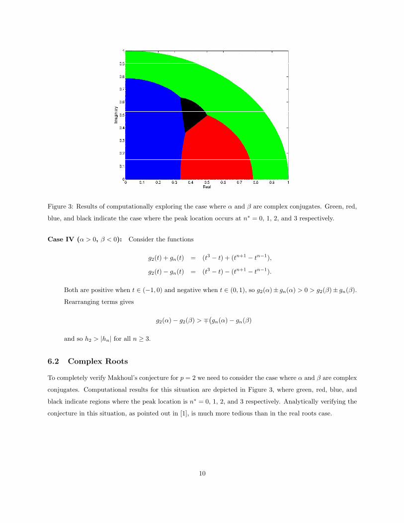
Figure 3: Results of computationally exploring the case where α and β are complex conjugates. Green, red,

blue, and black indicate the case where the peak location occurs at n∗ = 0, 1, 2, and 3 respectively.

Case IV (α > 0, β < 0): Consider the functions

g2(t) + gn(t) = (t3 − t) + (tn+1 − tn−1),

g2(t)− gn(t) = (t3 − t)− (tn+1 − tn−1).

Both are positive when t ∈ (−1, 0) and negative when t ∈ (0, 1), so g2(α)± gn(α) > 0 > g2(β)± gn(β).

Rearranging terms gives

g2(α)− g2(β) > ∓(gn(α)− gn(β)

and so h2 > |hn| for all n ≥ 3.

6.2 Complex Roots

To completely verify Makhoul’s conjecture for p = 2 we need to consider the case where α and β are complex

conjugates. Computational results for this situation are depicted in Figure 3, where green, red, blue, and

black indicate regions where the peak location is n∗ = 0, 1, 2, and 3 respectively. Analytically verifying the

conjecture in this situation, as pointed out in [1], is much more tedious than in the real roots case.

10

7 Investigating the Case of p = 3

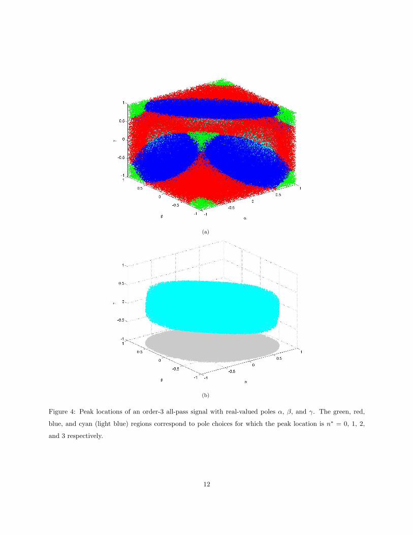
We have tried to get a feel for the third order situation using extensive computational efforts. It seems very

likely that Makhoul’s conjecture holds for p = 3. Figures 4(a) and (b), similar to previous figures, show

the peak location for various choices of three real-valued poles α, β, and γ. The red, green, blue, and cyan

(light blue) regions correspond to pole values for which the peak location is n∗ = 0, 1, 2 and 3 respectively.

Figure 4(b) shows only the values for n∗ = 3.

Comparing Figure 4 with Figures 1 and 2, we observe the following trend. Choices of real-valued poles

which result in a peak location at n∗ = 0 tend to be those near the extremities of the stable region, where

all poles have magnitude near unity. Similarly, placing all poles near the origin generally gives the largest

peak location achievable using only real-valued poles.

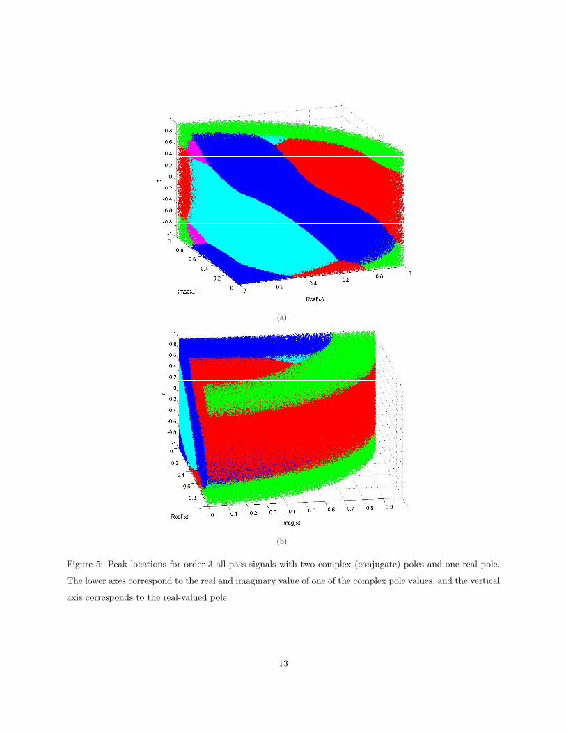
Our other observation is that maximal peak location achieved by any order-p all pass signal only occurs

when pairs of complex-valued poles are used. Figures 5(a) and (b), and Figure 6 depict the peak locations for

various pole choices using the same color scheme as in Figure 4, with black values corresponding to choices

which result in peak location at n∗ = 4. It seems that maximal peaks occur when complex poles are in the

range (0.6, 0.8) and the real-valued pole is again, near unity in magnitude. In either case, for higher order

filters I suspect that maximal peak locations will be attained only when complex-valued poles are used.

8 Bounds on the Peak Location

The matter at the heart Makhoul’s conjecture is finding a bound on the location of the last peak value of

an all-pass sequence as a function of the order p of the sequence. In their 1991 paper [4], Makhoul and

Steinhardt consider general causal signals with average delay τ defined as

τ =∑∞

k=0 kh2k∑∞

k=0 h2k

.

They establish that the peak location for causal signals with average delay τ is at most n∗ ≤ τ(τ +3)/2. They

also note that an order-p all-pass signal has average delay τ = p, so this gives a bound of n∗ ≤ p(p+3)/2 for

all-pass signals. Rajagopal and Wenzel improved upon this bound in [7] using properties of all-pass causal

signals to determine that

n∗ ≤ p√

2p + 1.

Boston suggests a more methodical approach to studying the peak location by first noting that the

recurrence relation representation of an impulse response for any order-p all-pass filter only depends fed-

back values for n ≥ p + 1 [1]. That is,

hn = −ap−1hn−1 − ap−2hn−2 − · · · − a1hn−p,

11

(a)

(b)

Figure 4: Peak locations of an order-3 all-pass signal with real-valued poles α, β, and γ. The green, red,

blue, and cyan (light blue) regions correspond to pole choices for which the peak location is n∗ = 0, 1, 2,

and 3 respectively.

12

(a)

(b)

Figure 5: Peak locations for order-3 all-pass signals with two complex (conjugate) poles and one real pole.

The lower axes correspond to the real and imaginary value of one of the complex pole values, and the vertical

axis corresponds to the real-valued pole.

13

0.20.3

0.40.5

0.60.7

0

0.2

0.4

0.6

0.8−1

−0.5

0

0.5

1

Real(α)Imag(α)

γ

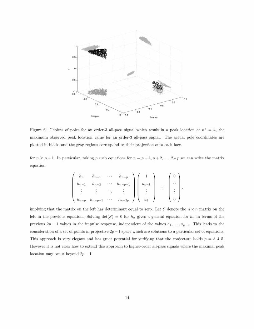
Figure 6: Choices of poles for an order-3 all-pass signal which result in a peak location at n∗ = 4, the

maximum observed peak location value for an order-3 all-pass signal. The actual pole coordinates are

plotted in black, and the gray regions correspond to their projection onto each face.

for n ≥ p + 1. In particular, taking p such equations for n = p + 1, p + 2, . . . , 2 ∗ p we can write the matrix

equation hn hn−1 · · · hn−p

hn−1 hn−2 · · · hn−p−1

......

. . ....

hn−p hn−p−1 · · · hn−2p

1

ap−1

...

a1

=

0

0...

0

,

implying that the matrix on the left has determinant equal to zero. Let S denote the n × n matrix on the

left in the previous equation. Solving det(S) = 0 for hn gives a general equation for hn in terms of the

previous 2p − 1 values in the impulse response, independent of the values a1, . . . , ap−1. This leads to the

consideration of a set of points in projective 2p−1 space which are solutions to a particular set of equations.

This approach is very elegant and has great potential for verifying that the conjecture holds p = 3, 4, 5.

However it is not clear how to extend this approach to higher-order all-pass signals where the maximal peak

location may occur beyond 2p− 1.

14

9 Counterexamples

As mentioned before, Makhoul’s conjecture breaks down at p = 6 where it is possible to have a peak location

at n∗ = 12 = 2p. Rajagopal and Wenzel discuss a heuristic strategy for maximizing the peak location [7].

Their strategy involves placing the poles near the border of the unit circle in a chirp-like pattern. This

agrees with the observation made in this paper, that maximal peak locations occur when complex pole-pairs

are used with magnitude not too near the origin. It is also interesting to note that the peak location is not

maximized when there are duplicate poles. Having the poles spread over a range of frequencies is preferable.

They also suggest that poles should cover a range of magnitudes (radii, measured from the origin) gradually

approaching the unit circle.

It would be interesting to characterize more precisely the location of peaks of all-pass signals, as no

precise characterization yet exists. It seems that traditional signal processing techniques (z-transform and

Fourier representations) do not lend themselves to properly characterizing these phenomena. To close with

a line borrowed from Rajagopal and Wenzel, “the field of all-pass filters offers many challenges for both

computational and theoretical approaches.”

References

[1] N. Boston. Makhoul’s conjecture for p = 2. In Proc. IEEE ICASSP, Salt Lake City, Utah, May 2001.

[2] J. Makhoul. Conjectured location of maximum amplitude in an all-pass sequence. SIAM Review,

28(3):395–397, Sep. 1986.

[3] J. Makhoul. Conjectures on the peaks of all-pass signals. IEEE Signal Processing Magazine, 17(3):8–11,

May 2000.

[4] J. Makhoul and A. Steinhardt. On the peaks of causal signals with a given average delay. IEEE Trans.

on Signal Processing, 39(3):620–626, March 1991.

[5] A. Oppenheim, R. Schafer, and J. Buck. Discrete-Time Signal Processing. Prentice-Hall, 1999.

[6] L. Rabiner and R. Crochiere. On the design of all-pass signals with peak amplitude constraints. Bell

Sys. Tech. J., 55(4):395–407, Apr. 1976.

[7] R. Rajagopal and L. Wenzel. Peak locations in all-pass signals – the Makhoul conjecture challenge. In

Proc. IEEE ICASSP, Salt Lake City, Utah, May 2001.

15