Discrete-Time Approximation for Nonlinear Continuous ...thesai.org/Downloads/Volume7No5/Paper_58-Discrete_Time... · Discrete-Time Approximation for Nonlinear ... discrete time model

(IJACSA) International Journal of Advanced Computer Science and Applications,

Vol. 7, No. 5, 2016

431 | P a g e

www.ijacsa.thesai.org

Discrete-Time Approximation for Nonlinear

Continuous Systems with Time Delays

Bemri H’mida

University of Tunis El Manar

National Engineers School of Tunis

Laboratory of Research on Automatic (LARA)

BP 37, Belvedere 1002 Tunis. Tunisia

Soudani Dhaou

University of Tunis El Manar

National Engineers School of Tunis

Laboratory of Research on Automatic (LARA)

BP 37, Belvedere 1002 Tunis. Tunisia

Abstract—This paper is concerned with the discretization of

nonlinear continuous time delay systems. Our approach is based

on Taylor-Lie series. The main idea aims to minimize the effect

of the delay and neglects the importance of nonlinear parameter

by the linearization of the system study in an attempt to make its

handling and easier programming as possible. We investigate a

new method based on the development of new theoretical

methods for the time discretization of nonlinear systems with

time delay .The performance of these proposed discretization

methods was validated by doing the numerical simulation using a

nonlinear system with state delay. Some illustrative examples are

given to show the effectiveness of the obtained results.

Keywords—Discrete-time systems; Time-delay systems; Taylor-

Lie series; non-linear systems; Simulation

I. INTRODUCTION

Research on discrete time delay systems has not attracted as much attention as that of continuous time delay systems. Many engineering applications need a compact and accurate description of the dynamic behavior of the considered system. This is especially true of automatic control applications. Dynamic models describing the system of interest can be constructed using the first principles of physics, chemistry, biology and so forth.

Time delay systems often appear in industrial systems and information networks. Thus, it is important to analyze time delay systems and design appropriate controllers. Control systems with time delays exhibit complex behaviors because of

their infinite dimensionality. Even in the case of linear time-invariant systems that have constant time delays in their inputs or states have infinite dimensionality if expressed in the continuous time domain. It is therefore difficult to apply the controller design techniques that have been developed during the last several decades for finite dimensional systems to systems with any time delays in the variables. Thus, new control system design methods that can solve a system with time delays are necessary.

As a result, controller design techniques developed for finite dimensional systems are difficult to apply to time delay systems with some effectiveness, time delay is often encountered in various engineering systems and its existence is frequently a source of instability. Many of these models are also significantly nonlinear which motivates research in the control of nonlinear systems with time delay. For this reasons, it’s difficult to analyze and design the control algorithm for the

nonlinear time delay system in the continuous time domain. It is necessary to develop a method to solve the time delay problem. Most of the proposed approaches deal with linear time-delay control systems and, in particular, with the stability analysis and behavior of such systems with constant and/or uncertain time delays [19,21,11]. Quite recently and on the nonlinear front, nonlinear controllers were systematically synthesized for multivariable nonlinear systems in the presence of sensor and actuator dead time [9,5].

In practice, most of industrial controllers are currently implemented digitally. In the design of model based digital control systems two general approaches can be identified. First, a continuous time controller is designed based on a continuous-time system model, followed by a digital redesign of the controller in the discrete time domain to approximate the performance of the original continuous time controller. Second, a direct digital design approach can be followed based on a discrete time model of the system, where the controller is now directly designed in the discrete time domain. It is apparent that this alternative approach has the attractive feature of dealing directly with the issue of sampling. We can emphasize, that in both design approaches time discretization of either the controller or the system model is necessary. Furthermore, note that in controller design for time delay systems the first approach is troublesome because of the infinite dimensional nature of the underlying system dynamics. As a result, the second approach becomes more desirable and will be pursued in the present study.

In particular, the well known procedure of time discretization of linear time delay systems [7,12,4] is extended to nonlinear input driven systems with constant time delay. All these approaches require a small time step in order to be deemed accurate, and this may not be the case in control applications where large sampling periods are inevitably introduced due to physical and technical limitations [13, 8]. Due to the physical and technical limitations, slow sampling has become inevitable. A time discretization method that expands the well known time discretization of linear time delay systems [1,6,2,3] to nonlinear continuous time control systems with time delays [10,17] can solve this problem. The effect of this approach on system theoretic properties of nonlinear systems, such as equilibrium properties, relative order, stability, zero dynamics, and minimum phase characteristics has also been studied [20,16] and reveals the natural and transparent manner in which Taylor methods permeate the


Vol. 7, No. 5, 2016

432 | P a g e


relevant theoretical aspects. A certainly not exhaustive sample of other approaches of notable significance, yet with certain associated practical limitations, are reported in [18], and solid theoretical results on the direct use of discrete time approximations in the control of sampled-data nonlinear systems can be found in [14,22].

In particular, the present study aims at the development of new methods for the time discretization of nonlinear input driven dynamic systems with time delay based on Taylor series. In particular, the paper is organized as follows: the next section contains some mathematical preliminaries; Section 3 discusses the discretization of system with internal point delay; Section 4 discusses the discretization of system with external point delay; Section 5 discusses the discretization of system with internal and external point delays; Section 6 discusses the linearization of nonlinear state space equation and a numerical example is given in section 7 to illustrate the proposed theoretical results and a concluding remark.

II. PRELIMINARIES

In the present study, single-input nonlinear continuous time control systems with input output time delays is considered using a state space representation of the form:

1 2 0 1 2 0 1

.( ) ( ( )) ( ( )) g ( ( )) ( ) g ( ( )) ( )t f x t f x t x t u t x t u tx

(1)

where,0

and 1 are the time delay and ( )u t is the control

input.

and0 1

( ) ( ).

( , )x f x t u t

(2)

wherenx R is the vector of the states representing an

open and connected set, u R is the input variable, m and

n are an integer which indicates the order of the input. 0

and

1 are the system constant time delay, that directly affects the

input and the state. It is assumed that:

:i

n nf R R and : n nig R R , i = 1; 2; ….

m and : n nf R R R are smooth mappings.

An equidistant grid on the time axis with mesh

10

k kT t t

is considered where sampling interval is

1[ , ] [ ,( 1) ]

kkt t kT k T

and T is the sampling period.

Furthermore, we suppose the time-delay 0

and 1 mesh T are

related as follows

0 0q T , (

01q , is an integer) (3)

1 1q T , (

11q , is an integer) (4)

where 0 1, 0,1,.....,q q m . That is, the time-delay

0 and

1 are customarily represented as an integer multiple of the

sampling period adding a fractional part of T [22].

It is assumed that system (1) is driven by an input that is piecewise constant over the sampling interval, i.e. the zero-order hold (ZOH) assumption holds true:

( ) ( ) ( )u t u kT u k =constant, for ( 1)kT t k T

(5)

III. DISCRETIZATION OF NONLINEAR SYSTEMS WITH

INTERNAL POINT DELAY

The nonlinear continuous time control systems with input time delay are considered using a state space representation form:

1 1 1

.( ) ( ( )) g ( ( )) ( )t f x t x t u tx

(6)

Based on the zero-order hold assumption and the above notation one can deduce that the delayed input variable attains the following two distinct values within the sampling interval:

1 1 1( ) ( ) ( )u t u kT q T u k q ,for ( 1)kT t k T

(7)

the nonlinear system (6) can be discretized using Taylor

series expansions over the subinterval ( 1)kT t k T and

taking into account (7), one can obtain the state vector

evaluated at ( 1)k T as a function of ( )x k and 1

( )u k q .

around the point0

( )x t , the state ( )x t can be expanded to

Taylor series as:

0 00 0 0 0 0

2 3''( ) '''( )( ) ( ) '( )( ) ( ) ( ) ...

2! 3!

x t x tx t x t x t t t t t t t

(8)

in the time interval1

[ , ] [ ,( 1) ]kk

t t kT k T , equation (8)

can be rewritten using equation (9):

2 3''( ) '''( )(( 1) ) ( ) '( ) ...

2! 3!

x kT x kTx k T x kT x kT T T T (9)

for simplicity and without misunderstanding, equation (9) can be rewritten as:

2 3''( ) '''( )( 1) ( ) '( ) ...

2! 3!

x k x kx k x k x k T T T

(10)

from equation (6), we can get the differential coefficient of

the state ( )x t :

1 1 1

.( ) ( ( )) g ( ( )) ( )t f x t x t u tx

(11)

then in the time interval1

[ , ] [ ,( 1) ]kk

t t kT k T , equation

(11) can be rewritten using equation (12):

1 1 1

.( ) ( ( )) g ( ( )) ( )k f x k x k u k qx

(12)

similarly, based on equation (6) we can calculate the

second derivative of the state ( )x t , shown in equation (13):

1 1 1

1 1 1

1 1

1 1 1

1 1

( ( ( )) ( ( ) ( )))( '( ))''( )

( ( )) ( ( )) ( )( ) ( ( ))

( ( )) ( ( )) ( )( ) ( ( ))

dxdx

dx d

d f x t g x t u td x tx t

dt dtdf x t dg x t du t

u t g x tdt dt

df x t dg x t du tu

x d

t g x tdx dx dt d

t

dx

t

(13)

for the zero order hold assumption, in each sampling interval


Vol. 7, No. 5, 2016

433 | P a g e


Equation (13) is correct:

1( )( )

0 0du tdu t

dx dx

(14)

then in each sampling interval, equation (13) can be expressed using equation (15):

1 1 1

1 1

1 1 1

1 1

1 1 1

( ( )) ( ( )) ( )( '( ))''( ) ( ) ( ( ))

( ( )) ( ( )) ( )( ) ( ( ))

( ( )) ( ) ( ( ))

df x t dg x t du td x tx t u t g x t

dt dx dx dt dt

df x t dg x t du t dxu t g x t

dx dx dx dt

f x t u t g x t dx

x

dx

dt

(15)

or1 1 1

.

( ) ( ( )) g ( ( )) ( )tdx

f x t x t u tdt

x ,

then equation (15) can be rewritten as:

1 1 1

1 1 1

1 1 1

(16)( ( )) ( ) ( ( ))( '( ))

''( )

( ( )) ( ) ( ( ))( ( )) ( )g ( ( ))

f x t u t g x td x t dxx t

dt x dt

f x t u t g x t

xf x t u t x t

in the time interval1

[ , ] [ ,( 1) ]kk

t t kT k T , equation (16)

can be rewritten using equation (17):

1 1 1

1 1 1

( ( )) ( ) ( ( ))''( ) ( ( )) ( )g ( ( ))

f x k u k q g x kx k

xf x k u k q x k

(17)

assume that:

1

1

1 1 1

1 1 1

1 1 1

1

2

1

( , )

( , )

( , )

( , )

( , )

( ( )) g ( ( )) ( )

( ( )) g ( ( )) ( )

( ( )) g ( ( )) ( )

1,2,3,...

l

A x u

x

A x u

x

l

A x u

A x u

A x u

f x k x k u k q

f x k x k u k q

f x k x k u k q

(18)

then equation (17) can be written as:

1

1 1 1

2

1 1 1

( ( )) ( ) ( ( ))''( )

( ( ), ( ))

( ( )) ( )g ( ( ))f x k u k q g x k

x kx

A x k u k q

f x k u k q x k

(19)

in the same way, we have:

3

1''' ( ( ), ( ))x A x k u k q

(20)

then equation (10) can be written as:

1

1

1

( ), ( )!

!( 1) ( )

( )N l

l

l l

l

l

l

N

tk

TA x k u k q

l

T d x

l dtx k x k

x k

(21)

here ( )x k is the value of the state ( )x t at the time t kT ,

1( ), ( )

lA x k u k q

can be calculated using equation (18).

The Taylor series expansion of equation (21) can offer either an exact sampled data representation of equation (6) by remaining the full infinite series representation of the state vector. It can also provide an approximate sampled data representation of equation (6) resulting from a truncation of the Taylor series order:

1

1

1

( ), ( )!

( 1) ( ), ( )

( )l

l

N

T

N l TA x k u k q

l

x k x k u k q

x k

(22)

where, the subscript of denotes the dependence of the sampling period and the superscript N denotes the finite series truncation order of the equation (22).

IV. DISCRETIZATION OF NONLINEAR SYSTEMS WITH

EXTERNAL POINT DELAY

The nonlinear continuous time control systems with state delay can be represented by the following state space form:

1 0 1 0

.( ) ( ( )) ( ( )) g( ( )) ( ) g ( ( )) ( )t f x t f x t x t u t x t u tx

(23)

where, 0

is the time delay and ( )u t

is the control input.

assume that in the time interval1

[ , ] [ ,( 1) ]kk

t t kT k T

0 0q T ,(

01q , is an integer)

In the time interval [ ,( 1) ]t kT k T , 0,1,..., 1k n ,

1 0( ( )) 0f x t and

1 0g ( ( )) ( ) 0x t u t . Under the

zero-order holds assumption and within the sampling interval,

the solution described in equation (23) is expanded in a

uniformly convergent Taylor series and the resulting

coefficients can be easily competed by taking successive partial

derivatives of the right hand side of equation (23). An approximate sampled data representation:

0

1

( ), ( )!

( 1) ( )l

l

N l TA x k q u k

lx k x k

(24)

where, ( , )l

A x u can be calculate using equation (23)

1

1

1 0 1 0

1 0 1 0

1 0 1 0

1

2

1

( , )

( , )

( , )

( , )

( , )

( ( )) g ( ( )) ( )

( ( )) g ( ( )) ( )

( ( )) g ( ( )) ( )

1,2,3,...

l

A x uq q

x

A x uq q

x

l

A x u

A x u

A x u

f x k q x k q u k

f x k x k u k

f x k x k u k

(25)

in the time interval [ ,( 1) ]t kT k T , 0,1,..., 1k n ,

equation (24) provides the approximates sampled data representation of equation (23):

1

0 !( ), ( ) ( ), ( )

!( 1) ( )

l

l lN l l T

l

TA x k u k B x k q u k

lx k x k

(26)


Vol. 7, No. 5, 2016

434 | P a g e


where, ( ), ( )l

A x k u k can be calculated using

equation(23), and 0( ), ( )

lB x k q u k

can be calculate using

equation (25):

1

1

1

1 0 1 0

2

1 0 1 0

1

1 0 1 0

( , )

( , )( , )

( , )( , )

( ( )) g ( ( )) ( )

( ( )) g ( ( )) ( )

( ( )) g ( ( )) ( )

1,2,3,...

l

B x u

B x uB x u q q

x

B x uB x u q q

x

l

f x k q x k q u k

f x k x k u k

f x k x k u k

(27)

The discrete time form of the nonlinear continuous system with state delay, shown in equation (23) can be gotten by combining equation (22) and (24).

V. DISCRETIZATION OF NONLINEAR SYSTEMS WITH

INTERNAL AND EXTERNAL POINT DELAYS

The nonlinear continuous time control systems with input output time delays are considered using a state space representation form:

1 0 1 0 1

.( ) ( ( )) ( ( )) g( ( )) ( ) g ( ( )) ( )t f x t f x t x t u t x t u tx

(28)

where, 0

and 1

are the time delays and ( )u t

is the control input.

assume that in the time interval1

[ , ] [ ,( 1) ]kk

t t kT k T

0 0q T , (


1 1q T , (


based on the zero order hold assumption and the above notation one can deduce that the delayed input variable attains the following two distinct values within the sampling interval:

1 1 1( ) ( ) ( )u t u kT q T u k q ,for ( 1)kT t k T

(29)

the nonlinear system (26) can be discretized using Taylor series expansions over the subinterval ( 1)kT t k T and

taking into account (27), one can obtain the state vector

evaluated at ( 1)k T as a function of 0

( )x k q and

1( )u k q .

in the time interval [ ,( 1) ]t kT k T , 0,1,..., 1k n ,

equation (24) provides the approximates sampled data representation of equation (23):

0 1( 1) ( ) ( ), ( ) ( ), ( )! !1

l lN l lT Tx k x k A x k u k B x k q u k ql ll

(30)

where, ( ), ( )l

A x k u k can be calculated using

equation(31), and 0 1( ), ( )

lB x k q u k q

can be calculate using

equation (32):

1

1

1

1 1

2

1 1

1

1 1

( , )

( , )( , )

( , )( , )

( ( )) g ( ( )) ( )

( ( )) g ( ( )) ( )

( ( )) g ( ( )) ( )

1,2,3,...

l

A x u

A x uA x u

x

A x uA x u

x

l

f x k x k u k

f x k x k u k

f x k x k u k

(31)

and:

1

1

1

1 0 1 0 1

2

1 0 1 0 1

1

1 0 1 0 1

( , )

( , )( , )

( , )( , )

( ( )) g ( ( )) ( )

( ( )) g ( ( )) ( )

( ( )) g ( ( )) ( )

1,2,3,...

l

B x u

B x uB x u q q

x

B x uB x u q q

x

l

f x k q x k q u k q

f x k x k u k q

f x k x k u k q

(32)

The discrete time form of the nonlinear continuous system with input output time delays, shown in equation (28) can be gotten by combining equation (22) and (24).

VI. LINEARIZATION OF NONLINEARSTATE EQUATION

The technique of linearization involves approximating a complicated system of equations with a simpler linear system. We hope to gain insight into the behavior of the nonlinear system through an analysis of the behavior of its linearization. We hope that the nonlinear system will behave locally like its linearization, at least in a qualitative sense.

In general, the linearization of a system of equations about an equilibrium point can be achieved by changing variables so that the equilibrium point is transformed to the origin. Points in the original system close to the equilibrium point will correspond to points close to the origin in the new system. Thus we are only concerned with values of the new variables close to zero and under certain conditions the nonlinear terms can be neglected. The equations that result are linear and are the linearization of the original system.

In order to linearize general nonlinear systems, we will use the Taylor Series expansion of functions.

Consider the nonlinear system:

( , )

( , )

x f x u

y g x u

(33)

with the equilibrium point is ( , )p q . Any function which is

differentiable can be written as a Taylor series expansion for

( , )f x u with neglect the terms of high order:

( , ) ( , )

.( , ) ( , ) ( ) ( ) ( , )

p q p q

f ff x u f p q x p u q F x u

x ux

(34)

where ( , )F x u consists of nonlinear polynomial terms in

( )x p and ( )u q .


Vol. 7, No. 5, 2016

435 | P a g e


since ( , )p q is an equilibrium ( , ) 0f p q and neglect high

order terms, then the state space representation form (33) can be rewritten as:

( , ) ( , )

.( , ) ( ) ( ) ( , )

p q p q

f ff x u x p u q F x u

x ux

(35)

for points near to the equilibrium point ( )x p and

( )u q are small and the non linear terms ( , )F p q can be

neglected.

We can write the state space model as:

( , ) ( , )

.( , ) ( ) ( )

p q p q

f ff x u x p u q

x ux

(36)

where the elements of linearization matrices are:

1 1

1 2( , ) ( , )

2 2( , )

1 2( , ) ( , )

p q p qi

i

j p q

p q p q

j

f f

x xfA

x f f

x x

,

1

( , )

2( , )

( , )

p qi

i

j p q

p q

j

f

ufB

u f

u

( , )

i

i

j p q

j

gC

x

and

( , )

i

i

j p q

j

gD

u

whereijA is called the Jacobian matrix.

VII. RESULT OF SIMULATIONS

The performance of the proposed methods of discretization for nonlinear systems with time delays is evaluated by applying it to a nonlinear continuous system with time delays. The partial derivative terms involved in the Taylor series expansion are determined recursively. The system considered in this paper is assumed to be a nonlinear control system, as it considers the pendulum equation with friction:

2

1 2

.

1

.

2

( , )( )

xf x u g k

sinx x u tl m

x

x

(37)

The vector ( )u t , called the input history or control input, is

chosen to influence the dynamics in some desired way. The

vector of functions f describes the system’s dynamics and the

vector of functions h provides a set of output measurements.

We call any pair ( ( ), ( ))x t u t satisfying over some time interval

including 0

( )t t a solution or trajectory.

Note that any system of higher order differential equations can be written in the first order form. For example, the motion of a simple pendulum with an input torque is described by the second order nonlinear equation:

0.2T s , 0.2s , 1g

l and 0,5

k

m

2

1 2

1

1 2

( , )0.5 ( 0.2)

0 1 0( 0.2)

0.5 1

xf x u

sinx x u t

xu t

sinx x

(38)

with:

1

2

xx

x

1

0 1

0.5A

sinx

0

1B

the Jacobian matrix of the function ( , )f x u of the

pendulum equation is given by:

1 1

1 2

2 2 1

1 2

0 1

cos( ) 0.5

f f

x xf

f f xx

x x

(39)

1

2

0

1

ff u

fu

u

(40)

evaluating the Jacobian matrix at the equilibrium points

(0, 0) and ( , 0) yields, respectively, the two matrices

1

0 1

1 0.5A

and

2

0 1

1 0.5A

The Taylor series expansion of equation (21) can offer either an exact sampled data representation of the equation (6) by remaining the full infinite series representation of the state vector. It can also provide an approximate sampled data representation of equation (6) resulting from a truncation of the Taylor series order:

( ), ( 1)( 1) ( ) A x k u k Tx k x k

(41)

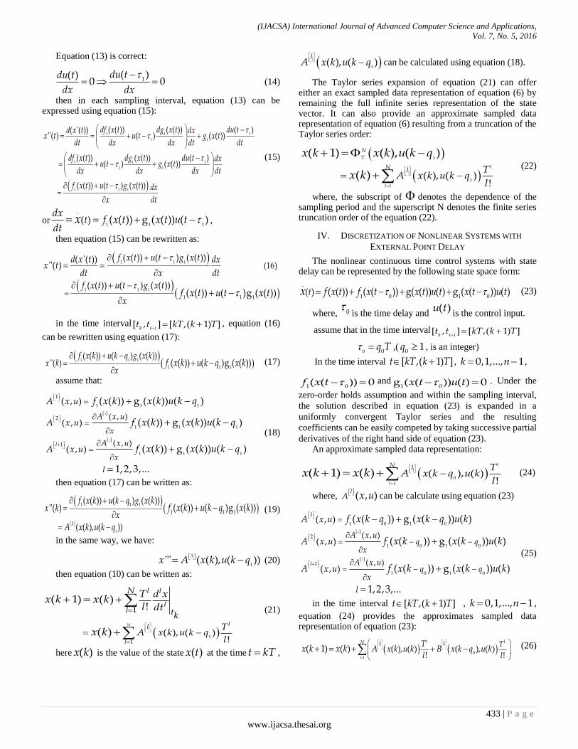
the simulation results is depicted in the figure 1


Vol. 7, No. 5, 2016

436 | P a g e


Fig. 1. Step response of nonlinear continuous and discret system with

control time delay

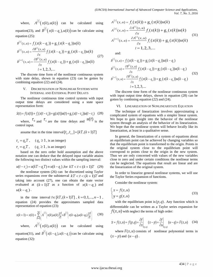
In the second case, the nonlinear continuous time control systems with state delay can be represented by the following state space form:

( 1), ( )( 1) ( ) A x k u k Tx k x k

(42)


Fig. 2. Step response of nonlinear continuous and discret system with state

time delay

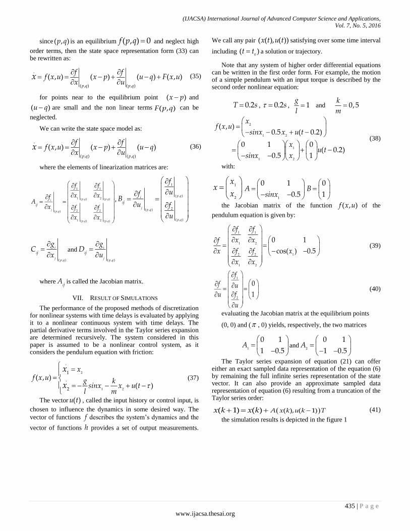
In the third case, the nonlinear continuous time control systems with input output time delays are considered using a state space representation form:

0 1

( 1) ( ) ( ), ( ) ( ), ( )x k x k A x k u k T A x k q u k q T

(43)


Fig. 3. Step response of nonlinear continuous and discret system with input

output time delay

Eventually, the simulation using a nonlinear system with time delay is conducted to validate the proposed time discretization method.

VIII. CONCLUSION

This paper proposed a time discretization method for nonlinear continuous systems with internal and external point delays. This proposed discretization method is based on Taylor series. The performance of the proposed time discretization method is evaluated using a nonlinear system with time delayed. The derived time discretization method provides a finite dimensional representation for nonlinear control systems with time delay, thereby enabling the application of existing nonlinear controller design techniques to such systems.

Finally, the simulation results show that the proposed discretization method does not change the original system stability nor increase much computational burden.

REFERENCES

[1] A. El moudni, b.bensassi: On a new order reduction method for discrete systems.12th world congress on scientific computation imacs,pp.95-99,1988.

[2] B.H'mida, M.Sahbi and S.Dhaou: Discrete-time approximation of multivariable continuous-time delay systems. IGI global handbook of research on advanced intelligent control engineering and automation, pp516-542, doi: 10.4018/978-1-4666-7248-2.ch019, January 2015.

[3] B.H'mida,M.Sahbi and S.Dhaou: Discretizing of linear systems with time-delay using method of euler's and tustin's approximations. International journal of engineering research and applications (ijera) ,issn: 2248-9622 , vol. 5 -issue 3, march 2015.

[4] B. H’mida, M. Sahbi and S. Dhaou: Stability of a linear discrete system with time delay via lyapunov-krasovskii functional. International journal of scientific research & engineering technology (ijset). Issn: 2356-5608, vol.3, issue 3, copyright cpco,pp .62-66, 2015.

[5] E. Fridman, U. Shaked, and V. Suplin., :Input/output delay approach to robust sampled-data h ∞ control.Systems& control letters, vol. 54, no. 3, pp. 271–282, 2005.

[6] J. Jugo.: Discretization of continuous time delay stems. 15th triennial word congress, d. Electricidad y electronica, f. De ciencias,upv/ehu,apdo.644,bilbao,barcelona, spainifac, 2002.

[7] L.s. Shieh, Yeung, C.k., and Mclnnis, B.C.: Solutions of state-space equations via block-pulse functions. Int. J. Control, 28, pp. 383-392,1978.

[8] M. Vidyasagar, Nonlinear Systems Analysis. Prentice Hall, Englewood Cliffs, NJ, USA.1978.

[9] N.k., Sinha and Lastman, G.J.: Transformation algorithm for identification of continuous-time multivariable systems from discrete data. Electron. Lett, 17, pp. 779-780,1981.

[10] N.ksinha and zouq. :Discrete time approximation of multivariable continuous time systems. Iee proceedings, vol 130,pt.d,n°3 ,pp 103-110,1983.

[11] 8S.MagdiMahmoud.:Robust filtering for time-delay systems. Marcel dekker,elsevier science inc. New york, ny, usa.an international journal,vol 176,isuue 2,pp.186-200,2000.

[12] W. Michiels, v. Van assche, and s.-i. Niculescu: stabilization of time-delay. Ieee transactions on automatic control, vol. 50, no. 4, april 2005.

[13] W. Michiels and S.-I. Niculescu . : Stability and stabilization of time-delay systems. An eigenvalue-based approach, ser. Advances in design and control. Vol. 12.,siam, 2007.

[14] Yuan-liang Zhang and Kil To Chong: Time-discretization of time delayed non-affine system via Taylor-lie series using scaling and squaring technique. International journal of control, automation, and systems, vol. 4, no. 3, pp. 293-301, june 2006.

[15] Y. L. Zhang, O. Kostyukova, K. T. Chong: A new time discretization for delay multiple-input nonlinear systems using the Taylor method and first

0 10 20 30 40 50 60-0.03

-0.02

-0.01

0

0.01

0.02

0.03

0.04

Time(sec)

Am

plitu

de

Step response

0 10 20 30 40 50 60-0.2

-0.15

-0.1

-0.05

0

0.05

Time(sec)

Am

plitu

de

Step response

0 10 20 30 40 50 60-0.4

-0.35

-0.3

-0.25

-0.2

-0.15

-0.1

-0.05

0

0.05

0.1

Time(sec)

Am

plitu

de

Step response


Vol. 7, No. 5, 2016

437 | P a g e


order hold. Discrete Applied Mathematics, vol. 159, no. 9, pp. 924-938, 2011.

[16] Y. L. Zhang: Discretization of nonlinear non-affine time delay system using first order hold assumption with scaling and squaring technique. International Review on Computers and Software, vol. 7, no. 4, pp. 1860-1865, 2012.

[17] Yuan-liang Zong : A discretization method for the nonlinear state delay system. Information technology journal, 13(6), pp.1222-1227, 2014.

[18] Yuan-Liang Zhang: Discretization of nonlinear non-affine time delay systems based on second-order hold. International journal of automation and computing, 11(3),pp 320-327 june 2014.

[19] Z. Kowalczuk.: Discrete approximation of continuous-time systems. A survey, proc. Iee-g,144, pp. 264–278, 1993.

[20] Zidong Wang, James lam, senior and Xiaohui Liu: Nonlinear filtering for state delayed systems with markovian switching. Ieee transactions on signal processing, vol. 51, no. 9, september 2003.

[21] Z. Qing-chang: Robust control of time-delay systems.Ieee transactions on automatic control ,53, pp. 636-637, 2008.

[22] Zheng Zhang and KilTo Chong: second order hold and Taylor series based discretization of siso input time-delay systems. Journal of mechanical science and technology 23 pp136-148, 2009.

Documents

Discrete-Time Approximation for Nonlinear Continuous ...thesai.org/Downloads/Volume7No5/Paper_58-Discrete_Time... · Discrete-Time Approximation for Nonlinear ... discrete time model