arX

iv:g

r-qc

/001

2035

v1 9

Dec

200

0

Discrete structures in gravity

Tullio Reggea) and Ruth M. Williamsb)

a) Dipartimento di Fisica, Politecnico di Torino,

Corso Duca degli Abruzzi, 10129 Torino, Italy.b) Girton College, Cambridge CB3 0JG, and

DAMTP, Silver Street, Cambridge CB3 9EW, United Kingdom.

May 28, 2018

Abstract

Discrete approaches to gravity, both classical and quantum, are reviewed briefly,with emphasis on the method using piecewise-linear spaces. Models of 3-dimensionalquantum gravity involving 6j-symbols are then described, and progress in gen-eralising these models to four dimensions is discussed, as is the relationship ofthese models in both three and four dimensions to topological theories. Finally,the repercussions of the generalisations are explored for the original formulationof discrete gravity using edge-length variables.

I Introduction to discrete gravity

A Basic formalism

The original motivation for the development of a discrete formalism for gravity[1] arose from a number of problems with the continuum formulation of generalrelativity. These included the difficulty of solving Einstein’s equations for gen-eral systems without a large degree of symmetry, the problems of representingcomplicated topologies and the need for considerable geometric insight and ca-pacity for visualisation. It turned out, as we shall see, that the discretisationscheme to be described not only helped with these problems but also found avital role in numerical relativity and in attempts at a formulation of quantumgravity.

The related branches of mathematics which found their application to physicsin this formulation of gravity are those of piecewise-linear spaces and topologyand the geometric notion of intrinsic curvature on polyhedra. The immedi-ate aim was to develop an approach to general relativity which avoided the

1

use of coordinates, since the physical predictions of the theory are coordinate-independent. The basic idea of the approach, which has subsequently becomeknown as Regge calculus, is as follows. Rather than considering spaces (orspace-times) with continuously varying curvature, we deal with spaces wherethe curvature is restricted to subspaces of codimension two. This is achievedby considering collections of n-dimensional blocks, which are glued together byidentification of their flat (n-1)-dimensional faces. The curvature lies on the(n-2)-dimensional subspaces, known as hinges or bones. For technical reasons,it is convenient to use blocks which are simplices (triangles, tetrahedra and theirhigher dimensional analogues).

Consider first the realisation of these ideas in two dimensions. Here wehave examples in everyday life, geodesic domes; these consist of networks offlat triangles which are fitted together to approximate curved surfaces, usuallyparts of a sphere. Since two triangles with a common edge can be flattenedout without distortion, there is no curvature on the edges. However, whena collection of triangles meeting at a vertex is flattened, there will be a gap,indicating the presence of curvature at the vertex. The amount of curvaturethere depends simply on the size of the gap or deficit angle.

It is relatively simple to visualise the generalisation of a triangulated surfaceto three dimensions, where a collection of flat tetrahedra are glued together ontheir flat triangular faces. In general, the tetrahedra at an edge will not fittogether exactly in flat space, so there will be a deficit angle at that edge givinga measure of the curvature there. In four dimensions, the curvature is restrictedto the triangles between the tetrahedra where the four-simplices meet. And soon in higher dimensions. Thus we have a set of flat simplices glued together toapproximate a curved space.

There is another way of viewing the scheme that has just been described.Piecewise-flat spaces are interesting in their own right, so in addition to usingthem as an approximation scheme for some curved “reality”, we may also studysuch spaces for their own sake. It has been argued (for example by Friedberg andLee [2]) that space-time is actually discrete at the smallest scales, so one couldalso regard curved spaces as approximations to a discrete reality. A chacun sesgouts!

In order for the piecewise-flat spaces to be of any practical use in relativity,beyond ease of visualisation, it must be possible to calculate geometric quantitieslike curvature and volume, and in particular to evaluate the Einstein action ofsuch a space. In [1] it was shown heuristically that the analogue of the Einsteinaction

I =1

2

∫

R√gdnx, (1)

is given by

IR =∑

hinges i

|σi|ǫi (2)

where |σi| is the measure of a hinge σi and ǫi is the deficit angle there, equalto 2π minus the sum of the dihedral angles between the faces of the simplices

2

meeting at that hinge. Rigorous justification for this formula followed in [3],where it was shown that it converges to the continuum form of the action, inthe sense of measures, provided that certain conditions on the fatness of thesimplices are satisfied. Friedberg and Lee [4] approached the problem from theopposite direction, deriving the Regge action from a sequence of continuumspaces approaching a discrete one.

The reason for choosing the building blocks to be simplices is that the geom-etry of a flat simplex is completely determined by the specification of its edgelengths, so a simplicial space may be described exactly by these lengths withoutthe need for any further variables like angles. This means that the simplestchoice of variables for the discrete theory is the edge lengths; clearly the actionmay be calculated once they are specified and they are also the obvious ana-logues of the metric tensor, which serves as variable in the continuum theory.There, an elegant way of deriving Einstein’s equations is from the principle ofstationary action, varying I with respect to the metric. The analogue in Reggecalculus is to vary IR with respect to the edge lengths, giving the simplicialequivalent of Einstein’s equations:

∑

i

∂|σi|∂lj

ǫi = 0, (3)

where we have used the result in [1], that the variation of the angular termsgives zero when summed over each simplex (Schlafli’s differential identity).

At first sight, it appears that there is one equation for each variable, promis-ing the possibility of a complete solution for the edge lengths. However thesituation is not as simple as that; there are analogues of the Bianchi identitiesin Regge calculus [1, 5, 6, 7, 8], which in the case of flat space provide exactrelations between sets of equations, and approximate relations in the nearly-flatcase, so the equations may not provide sufficient information for a completesolution. In that case there is freedom to specify certain variables, in analogywith the freedom to specify lapse and shift in the 3+1 version of continuumgeneral relativity.

B Classical applications

In the ten years after its formulation, Regge calculus was applied almost exclu-sively to problems in classical relativity, in particular to the time developmentof simple model universes. (Rather than give a complete list of references here,we refer the reader to the bibliography [9] which contains a comprehensive listfor the first 20 years.) The basic idea was really 3+1 in nature: take a trian-gulation of a 3-dimensional surface (usually closed but not necessarily so) torepresent a hypersurface at a particular moment of time and join its vertices tothe corresponding vertices of a second 3-dimensional triangulation, representingthe same hypersurface at a later time. The edges used to join these verticesare taken to be timelike and the slice of 4-dimensional space-time between thetwo triangulations is then divided into 4-simplices by inserting appropriate di-agonals. Given the edge lengths on the first 3-d triangulation, and specifying

3

the timelike edge lengths, the Regge equations may in principle be solved forthe edge lengths on the second 3-d triangulation. By repetition of this process,the classical evolution of the inital spacelike surface may be calculated. Thissounds simple enough, but unless quite strong assumptions of symmetry aremade, the numerical calculation, involving large sets of simultaneous equationsfor the edge lengths, can be very time-consuming and complicated.

Significant progress with this approach was made in the early nineties when,based on an idea of Sorkin [10], it was realised that in general, the Regge equa-tions decouple into a collection of much smaller groups. These groups of equa-tions can then be solved in parallel, which means that the computer time re-quired for an equivalent calculation is much less. This parallelisable implicitevolution scheme is described in detail in [11] and the basic mechanism is asfollows. Consider a single vertex in a triangulated 3-dimensional spacelike hy-persurface and introduce a new vertex “above” this. Connect the new vertex bya “vertical” edge to the chosen vertex, and by “diagonal” edges to all the ver-tices in the original hypersurface to which the chosen vertex was joined. Eachtetrahedron in the original surface now has based on it a 4-simplex, with apexat the new vertex. Note that there is one diagonal corresponding to each edgein the original vertex radiating from the chosen vertex. We now use the Reggeequations for these edges in the original surface and for the vertical edge; theonly unknown edges which these equations involve are the new vertical edgeand the diagonal edges, and there is precisely the same number of equationsas unknowns. Thus, in principle, we can solve exactly for the unknown edgelengths. (In practice, because of the approximate relationship between the equa-tions from the Bianchi identities, it is often more convenient to ignore some ofthe equations and instead specify conditions equivalent to the lapse and shift.)

We have described how to evolve vertices one-by-one in the Sorkin evolutionscheme, and the entire hypersurface can be evolved in this way. The methodis very general and can be used for a hypersurface with arbitrary topology.However, advancing the vertices one-by-one will not ordinarily be the mostefficient way of evolving a hypersurface. If any two vertices in a hypersurfaceare not connected by an edge, then they can be evolved to the next surface atthe same time without interfering with each other, which is why the method isobviously parallelisable.

C Some quantum applications

The earliest application of Regge calculus to quantum gravity was in three di-mensions [12] and involved 6j-symbols. This work, and subsequent developmentsalong those lines, will be the subject of the next two main sections and we shallnot discuss it further here.

¿From the early eighties onwards, there have been many attempts to for-mulate a theory of quantum gravity based on Regge calculus, and we shallsummarise the salient features of some of those approaches, both analytic andnumerical.

The first work on quantum Regge calculus in four dimensions involved using

4

a study of small perturbations about a flat background to relate the discretevariables with their continuum counterparts [13]. The discrete propagator wasderived in the Euclidean case and shown to agree with the continuum propagatorin the weak field limit. (More details of this calculation will be given in thesection on area Regge calculus.) The technique of weak field approximation hasproved to be very useful not only for comparisons with the continuum theorybut also as a guide in numerical calculations.

The difficulties of analytic calculations in quantum Regge calculus, coupledwith the need for a non-perturbative approach and also the availability of so-phisticated techniques developed in lattice gauge theories, have combined tostimulate numerical work in quantum grvity, based on Regge calculus. One ap-proach is to start with a Regge lattice for, say, flat space, and allow it to evolveusing a Monte Carlo algorithm (see for example [14, 15, 16]). Random fluctu-ations are made in the edge lengths and the new configuration is rejected if itincreases the action, and accepted with a certain probability if it decreases theaction. The system evolves to some equilibrium configuration, about which itmakes quantum fluctuations, and expectation values of various operators can becalculated. It is also possible to study the phase diagram and search for phasetransitions, the nature of which will determine the vital question of whether ornot the theory has a continuum limit. Many of the simulations have involvedan action with an extra term, quadratic in the curvature, to avoid problems ofconvergence of the functional integral; some have included scalar fields coupledto gravity [17]. Recent work by Riedler and collaborators in four dimensions de-scribes evidence for a new continuous phase transition, essential for a continuumlimit, at negative gravitational coupling [18].

The choice of measure in the functional integral is still a matter for contro-versy, depending both on attitude to simplicial diffeomorphisms and also on thestage at which translation from the continuum to the discrete takes place. Thenumerical simulations just described mainly use a simple scale invariant mea-sure [19]. Menotti and Peirano have derived an expression for the functionalmeasure in 2-dimensional Regge gravity, starting from the DeWitt supermetric,and giving exact expressions for the Fadeev-Popov determinant for both S2 andS1xS1 topologies (see [20] and references therein).

A rather different approach to numerical simulations of quantum gravity isthat of dynamical triangulations. (For a review containing an extensive set ofreferences, see [21]). This also uses Regge lattices and the Regge action, butthere are important differences. In the traditional approach, we are effectivelyintegrating over the edge lengths in the functional integral, but in dynamicaltriangulations, the lattice is taken to be equilateral, with a certain length scale,and the summation is over different triangulations, which are generated by a setof (k,l) moves [22]. In two dimensions, there are just two possible moves (andtheir inverses): the reconnection of vertices in two triangles with a commonedge, and the insertion of a vertex and edges in a triangle to divide it intothree triangles (2-2 and 1-3 moves). There are straightforward generalisationsof these moves to higher dimensions. The moves are ergodic in the sense that anycombinatorially equivalent triangulation can be generated by a finite succession

5

of these moves. It is argued that the restiction to equilateral triangulationsis a way of avoiding over-counting gauge-related configurations. The approachhas been very successful in two dimensions, where there are analytic resultswith which to compare the calculations. In three and four dimensions, therehas been progress in, for example, deriving the crucially important exponentialbound on the number of triangulations for a given number of vertices [23], butthere are still open questions on the continuum limit, since the phase transitionappears to be first order (see the review by Loll [24]). Recently a Lorentzianversion of dynamical triangulations has been formulated in (1+1)-dimensions[25]. Numerical simulations have revealed a new universality class for puregravity, with Haussdorf dimension two.

Discrete gravity has also proved very useful in calculations of the wave func-tion of the universe [26]. According to the Hartle-Hawking prescription, thewave function for a given 3-geometry is obtained by a path integral over all4-geometries which have the given 3-geometry as a boundary. To calculate suchan object in all its glorious generality is impossible, but one can hope to capturethe essential features by integrating over those 4-geometries which might, forwhatever reason, dominate the sum over histories. This has led to the conceptof minisuperspace models, involving the use of a single 4-geometry (or perhapsseveral). In the continuum theory, the calculation then becomes feasible if thechosen geometry depends only on a small number of parameters, but anythingmore complicated soon becomes extremely difficult. For this reason, Hartle [27]introduced the idea of summing over simplicial 4-geometries as an approxima-tion tool in quantum cosmology. Although this is an obvious way of reducingthe number of integration variables, there are still technical difficulties: the un-boundedness of the Einstein action (which persists in the discrete Regge form)leads to convergence problems for the functional integral, and it is necessary torotate the integration contour in the complex plane to give a convergent result[28, 29].

In principle, the sum over 4-geometries should include not only a sum overmetrics but also a sum over manifolds with different topologies. One then runsinto the problem of classifying manifolds in four and higher dimensions, whichled Hartle [30] to suggest a sum over more general objects than manifolds,unruly topologies. Schleich and Witt [31] have explored the possibility of usingconifolds, which differ from manifolds at only a finite number of points, andthis has been investigated in some simple cases [32, 33]. However, a sum overtopologies is still very far from implementation.

Yet another area of application of Regge calculus in quantum gravity involvesthe study of the simplicial supermetric, the metric on the space of 3-geometries.Its signature is crucial for determining spacelike surfaces in superspace, whichare important in Dirac quantisation and in quantum cosmology. In the contin-uum, there are limited results on the signature and this led to the possibility ofinvestigating it in the discrete case [34], where the analogue is the Lund-Reggesupermetric [35]. This supermetric was constructed for some simple manifolds(S3 and T 3) and its signature calculated. The results agreed with the continuumpredictions and also showed that the supermetric can become degenerate. We

6

still do not have a complete understanding of the division of the modes into “ver-tical” (corresponding to metrics related by diffeomorphisms) and “horizontal”ones.

D Other approaches to discrete gravity

Of course Regge calculus is not the only way of setting up a theory of discretisedgeneral relativity. In this subsection, we shall describe some alternatives.

One important class of schemes involves treating gravity as a gauge the-ory. For example, Mannion and Taylor [36] defined a theory of gravity on afixed hypercubic lattice, and Kaku [37] used a fixed random lattice. Howevera dynamical lattice seems more appropriate in a theory aiming to describe thequantum fluctuations of space-time, and this was used in much earlier work byWeingarten [38].

In an approach closely related to Regge calculus, Caselle, D’Adda and Mag-nea [39] defined a theory of gravity on the dual lattice, giving both first- andsecond-order formulations. The action they obtained was a compactified formof the Regge action, involving the sine of the deficit angle. D’Adda and Giontishowed [40] that Regge calculus is a solution of the first order formulation inthe limit of small deficit angles. The action of Caselle, D’Adda and Magnea wasalso used by Kawamoto and Nielsen [41] in their version of lattice gravity withfermions.

Immirzi investigated the links between canonical general relativity in thecontinuum, loop quantum gravity, and spin networks, in an attempt to formulatea quantised version of discrete gravity in the spirit of Regge calculus but raninto problems over hermiticity [42].

A totally different approach to discrete gravity is ’t Hooft’s polygon modelin (2+1)-dimensions [43]. This was introduced as a way to refute Gott’s claimof acausality in (2+1) gravity coupled to point particles [44]. ’t Hooft’s methodis to split space-time into the direct product of cosmological time and a Cauchysurface tessellated by flat polygons. The local flatness of space-time in the puregravity regime and the cone-like structure introduced by particles, as in Reggecalculus [45], are expressed in terms of conditions on the edges and verticesof the polygons. A local Lorentz frame is attached to each polygon and twoconstraints imposed; these are firstly that time runs at the same rate in eachpolygon (which corresponds to a partial gauge fixing) and secondly that allvertices are trivalent (which is acceptable because higher order vertices canalways be split into trivalent vertices connected by edges of zero length). Theconsequences of these conditions are that the length and velocity of an edge arethe same in both polygons to which it belongs, and that the velocity of eachedge is orthogonal to it in both frames. These facts result in transition rules forthe vertices in the tessellation.

The method for evolving such a space-time is as follows. Initial data (lengthsand velocities), subject to consistency conditions, are assigned to the edges on apolygonally-tessellated hypersurface. The configuration evolves linearly until anedge collapses to zero length or a vertex crosses another edge. A transition, gov-

7

erned by the vertex conditions, then takes place to another configuration whichwill, in general, have different numbers of vertices, edges and polygons. Thenew data will still satisfy the consistency conditions and the process is then re-peated. When there are particles present at the vertices, there are deficit anglesproportional to their masses, and the transition rules are modified accordingly.

It is not an easy task to follow the time-evolution of a (2+1)-dimensionalmodel with particles, even though the system has a finite number of degrees offreedom. ’t Hooft did numerical simulations on a small computer, with someunexpected predictions. His big-bang and big-crunch hypotheses were based onthe evolution of a Cauchy surface with S2 or S1xS1 topology, tessellated by asingle polygon [46]. It would be interesting to test these predictions for morecomplex initial configurations, and as a means to this, there has been recentwork [47] in which the constraint equations have been interpreted in terms ofhyperbolic geometry (see also [48]), and various consistent sets of initial dataset up, but the evolution calculations have not yet been completed. Part of themotivation for this work is to compare ’t Hooft’s method with other approachesto (2+1) gravity, in particular Regge calculus. A (2+1)-dimensional code hasbeen set up for Regge space-times and a number of calculations performed [49],with a view to making detailed comparisons with the ’t Hooft method. The ul-timate aim is to understand the exact relationship between the two approaches,which seem rather different but have many concepts in common.

Based on the polygon approach, various toy models of (2+1)-dimensionalgravity have been constructed [46, 50], issues of topology been addressed [50,51] and particle decay and space-time kinematics been investigated [52]. ’tHooft himself has proposed quantised models of (2+1)-dimensional space-time[53], showing that gravitating particles live on a space-time lattice. For anS2xS1 topology, first quantisation of Dirac particles is possible. Waelbroeck hassuggested a similar approach, using canonical quantisation in (2+1) dimensions[54].

Back at the classical level, Brewin has formulated [55] a discretisation ofgravity which he feels is closer to the original theory of general relativity. Pre-liminary calculations are encouraging. For other important work on latticegravity by Bander, Jevicki and Ninomiya, Khatsymovsky and Lehto, Nielsenand Ninomiya, we refer the reader to the Regge calculus review and bibliogra-phy [9]. We emphasise again that this paper is not meant to be an exhaustivereview of the subject.

After this rather rapid survey of applications of Regge calculus, and someother approaches to discrete gravity, we shall now concentrate on one particularapproach and show how it has led to exciting new developments in the searchfor a quantum theory of gravity.

2. 6j-symbols in 3-dimensional quantum gravity

As promised, we now look in detail at the earliest link forged between Reggecalculus and quantum gravity, now known as the Ponzano-Regge model [12].

8

This emerged from a paper on 6j-symbols and we will first give the backgroundto these.

A 6j-symbols

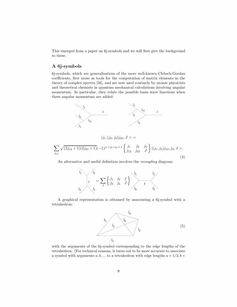
6j-symbols, which are generalisations of the more well-known Clebsch-Gordancoefficients, first arose as tools for the computation of matrix elements in thetheory of complex spectra [56], and are now used routinely by atomic physicistsand theoretical chemists in quantum mechanical calculations involving angularmomentum. In particular, they relate the possible basis wave functions whenthree angular momentum are added:

j1

Jj12

j3

J

j23

j1

2j

3j

j2

|j1, (j2, j3)j23, J > =

∑

j12

√

(2j12 + 1)(2j23 + 1)(−1)j1+j2+j3+J

{

j1 j2 j3j12 j23 J

}

|(j1, j2)j12, j3, J >.

(4)An alternative and useful definition involves the recoupling diagram:

j2

4j j3

j1

j =∑

J

{

j1 j2 jj3 j4 J

}

j1

j2

4j j3

J

A graphical representation is obtained by associating a 6j-symbol with atetrahedron:

j1

j4

j5

j3

j6

j2

(5)

with the arguments of the 6j-symbol corresponding to the edge lengths of thetetrahedron. (For technical reasons, it turns out to be more accurate to associatea symbol with arguments a, b, ... to a tetrahedron with edge lengths a+1/2, b+

9

1/2, ....) For the 6j-symbol to be non-zero, the arguments have to satisfy theanalogue of the triangle inequalities for each face of the tetrahedron:

j3 ≤ j1 + j2 etc (6)

They can be evaluated from the formula{

a b cd e f

}

=√

∆(a, b, c)∆(a, e, f)∆(c, d, e)∆(b, d, f)

∑

x

(−1)x(x+ 1)![(a+ b+ d+ e− x)!(a+ c+ d+ f − x)!(b + c+ e+ f − x)!

(x− a− b − c)!(x− a− e− f)!(x− c− d− e)!(x− b− d− f)!]−1 (7)

where

∆(a, b, c) = (a+ b− c)!(b+ c− a)!(c+ a− b)![(a+ b+ c+ 1)!]−1. (8)

These 6j-symbols are based on the group SU(2), but as we shall see, it is alsopossible to have q-deformed 6j-symbols based on quantum groups. For example,define [57]

q = exp(2πi/r) (9)

and

[n] =(qn/2 − q−n/2)

(q1/2 − q−1/2). (10)

Then the q-deformed 6j-symbol for SUq(2) is defined in the same way asthe undeformed one, with n replaced everywhere by [n]. Note that [n] → n asq → 1 and r → ∞.

B The Ponzano-Regge model

The main purpose of the paper by Ponzano and Regge [12] was to derive asymp-totic formulae for classical (ie undeformed) 6j-symbols in the limit when certainarguments became large. The case most relevant to the exposition here is whenall six parameters become large. The edge lengths of the corresponding tetrahe-dron are really related to jih and these quantities are kept finite as ji → ∞ whileh → 0 so this process corresponds to the semi-classical limit. This asymptoticbehaviour is given by

{

j1 j2 j3j4 j5 j6

}

∼ 1

12πVcos(

∑

i

jiθi + π/4) (11)

where V is the volume of the terahedron and θi is the exterior dihedral angleat edge i (ie the angle between the outward normals to the faces meeting there).This was recently proved rigorously by Roberts [58].

10

To see the connection between this formula and quantum gravity, considerthe following state sum defined in [12]. Take a closed 2-dimensional surface,triangulate it and divide its interior into tetrahedra, possibly inserting internalvertices. Label the internal edges by xi and the external ones by li. Define

S({li}) =∑

xi

∏

tetrahedra

{6j}(−1)X∏

i

(2xi + 1) (12)

where the X in the phase factor is a function of the edge lengths.Although this expression is infinite in many cases, it has some extremely

interesting properties. In particular, noting that in the sum over the internaledges, the large values dominate, we can replace the sum by an integral withrespect to those edge lengths and use the asymptotic formula stated above. Thenthe dominant contribution to the integral comes from the points of stationaryphase, which are given by

∑

tetrahedra k meeting on edge i

(π − θki ) = 2π. (13)

This means that the sum of the dihedral angles at each edge is 2π, whichis precisely the condition for local flatness in a 3-dimensional simplicial space.What is more, the state sum is given approximately by

S ≈ 1√12π

∫

∏

i

dxi(2xi + 1)(−1)X∏

tet k

1√Vk

cos(∑

l∈tet k

jlθkl +

π

4). (14)

Now this contains a term of the form∫

∏

i

dxi(2xi + 1)exp(i∑

edges l

jl(2π −∑

tet k∋i

(π − θkl )) =

∫

∏

i

dxi(2xi + 1)exp(i∑

jlǫl), (15)

which looks precisely like a Feynman sum over histories with the Reggecalculus action in three dimensions:

∫

∏

i

dµ(xi)exp(iIR) (16)

with

IR =∑

l

jlǫl, (17)

where ǫl is the deficit angle at edge l and dµ(xi) is the measure on the spaceof edge lengths.

This result was rather puzzling and, although Hasslacher and Perry [59]emphasised the connection between spin networks and simplicial gravity, itssignificance was not fully appreciated until much later, when a very similarexpression was written down in a different context.

11

C The Turaev-Viro model

In the late eighties and early nineties, mathematicians put a lot of effort intosearching for invariants of manifolds, the hope being, at least in part, that suchquantities would help with the classification of manifolds. Without being awareof the Ponzano-Regge work, Turaev and Viro [60] defined a state sum for tri-angulated 3-manifolds, which in many aspects was identical to that of Ponzanoand Regge. The main differences were that they gave formulae for closed man-ifolds as well as those with boundary, they showed explicitly that the quantityobtained was independent of triangulation, and finally, they used 6j-symbols forthe quantum group SLq(2). Only some of the irreducible representations of thisgroup, the ones with j taking finite values, have suitable algebraic properties,which means that the edge lengths are not summed up to infinite values; ji cantake only integer and half-integer values from the set (0, 1/2, 1, ..., (r − 2)/2),with r ≥ 3. A very important consequence of this is that the answer obtainedis finite, and so the model appears to be a regularised version of the Ponzano-Regge model.

The obvious question to ask is how the Turaev-Viro state sum is connected toquantum gravity. Witten [61] conjectured that it was equivalent to a Feynmanpath integral with the Chern-Simons action for SUk(2)

⊗

SU−k(2), and thisand equivalent results were proved by a number of people [62, 63, 64]. To seehow this works [65, 66], consider the Chern-Simons Lagrangian for this groupproduct:

L =k

4π

∫

M

Tr(A+ ∧ dA+ +2

3A+ ∧ A+ ∧ A+)

− k

4π

∫

M

Tr(A− ∧ dA− +2

3A− ∧ A− ∧ A−) (18)

where

A± = Aai (±)Tadxi (19)

with Ta a basis of the SU(2) Lie algebra. Making the change of variables

Aai (±) = ωa

i ± 1

keai , (20)

where eai is the dreibein and

ωai =

1

2ǫabcωibc, (21)

with ωibc being the connection 2-form, we obtain

∫

(e ∧R+λk

3e ∧ e ∧ e), (22)

which is the Einstein-Hilbert action for gravity with cosmological constantgiven by

12

λk = (4π

k)2. (23)

(Note that the k here is equal to r − 2, where r appears in the definition ofq.) By taking the limit as k → ∞, we obtain 3-dimensional gravity with zerocosmological constant ie the theory represented by the Ponzano-Regge model.This result is consistent with the fact that the q → 1 limit of the Tuaev-Viromodel is the Ponzano-Regge model.

The properties of the Turaev-Viro state sum show that the formalism is anexample of a topological quantum field theory (see eg [67]). This is perfectlyappropriate for a theory of gravity in three dimensions where there are no localdegrees of freedom. As for the Ponzano-Regge theory, the dominant classicalconfigurations are locally flat (recall that in Chern-Simons gravity, the solutionsinvolve the space of flat connections.)

The relationship between the Turaev-Viro invariant and 3-dimensional quan-tum gravity is an extremely important one. It means that in three dimensions,we have in principle a way of calculating the partition function for triangu-lated manifolds. This has been done for many of the simpler 3-manifolds (see[68, 69] for example). The Turaev-Viro expression can also be used for calculat-ing topology-changing amplitudes in 3-dimensional gravity; the method here isto construct a cobordism between two 2-dimensional triangulated surfaces andthen use the Turaev-Viro expression for a manifold with boundaries to evaluatethe transition probability [70].

D Spin networks

The Turaev-Viro expression is not the only method of calculating this particularinvariant of 3-manifolds. Various other prescriptions have been written down,and one that is worth describing at this stage is that using spin networks. Thesewere invented by Penrose [71] who wanted to formulate a purely combinatorialapproach to space-time. His networks had trivalent vertices and the edges ofthe graphs were labelled by spins. He developed a method of calculating thevalue of an arbitrary spin network and was able to show that this led to theusual angles of 3-dimensional space.

Penrose’s spin networks were later generalised in a number of ways. Theedges were labelled by representations of quantum groups and it was necessaryto introduce intertwining operators or intertwiners at the vertices [72]. In somecases a framing was introduced and the graphs became ”ribbon graphs” [73].Kauffman [74] showed how to calculate the Turaev-Viro invariant by taking thegraph dual to a triangulation to be a spin network; the edges of the graph inheritthe labels of the triangulation edges which they cross. Spin networks have alsobeen introduced into loop quantum gravity [75], where they are an importantcalculational tool, for instance in the derivation of the spectrum of the areaand volume operators [75]. (Note that Freidel and Krasnov also obtained adiscrete spectrum for the volume operator in BF theory by differentiating theTuraev-Viro amplitude with respect to the cosmological constant [76].) As we

13

shall see, spin networks also play a role in recent attempts at formulations of4-dimensional quantum gravity.

III Extensions to four dimensions

After it was realised that the Turaev-Viro state sum provides a finite theory of3-dimensional gravity, the search began for a generalisation to four dimensions.Before this is described, we shall stop to ask what we hope to achieve by this. Inclassical general relativity, there are enormous qualitative differences betweengravity in three and four dimensions. In particular, there are gravitons in fourdimensions, but not in three, so although it seems reasonable to describe 3-dimensional gravity by a topological invariant of a manifold, it seems likelythat an invariant of a 4-manifold might describe only some topological sector ofgravity. We shall return to this point later.

The obvious way of setting about extending the 3-dimensional model, basedon 6j-symbols, to four dimensions is by using some 3nj-symbol for a value ofn larger than 2. The 3nj-symbols in the state sum would then be expandedin terms of 6j-symbols, and the Ponzano-Regge formula for their asymptoticvalues inserted, the hope being that this would give an expression looking likea path integral with the 4-dimensional Regge action. The problem with this isthat the asymptotic formula involves the 3-dimensional dihedral angles and itis very difficult to relate these to 4-dimensional angles. This indicates that amore radical generalisation may be needed.

We shall now describe some of the attempts at generalisation, leading up tosome recent work which seems very promising.

A The Ooguri model

A source of inspiration for some generalisations of the Ponzano-Regge andTuraev-Viro models was Boulatov’s generalised matrix model [77], which in-volved a scheme for generating 3-dimensional simplicial complexes as terms ina perturbative expansion. The contribution from each simplicial-complex wasweighted by its Ponzano-Regge or Turaev-Viro invariant, depending on the valueof q. Boulatov’s model was formulated in a way that it could be extended tohigher dimensions, and the 4-dimensional case for q = 1 was worked out byOoguri [78].

The essential ingredients in Ooguri’s model are the assigning of group vari-ables to the tetrahedra and spin j labels to the triangles in the triangulated4-manifold. The terms in Ooguri’s action are of two types: the first is a productof two functions of the group variables, and this represents two glued tetrahe-dra; the second is a product of five functions and represents the tetrahedra in a4-simplex. A Fourier decomposition is performed in terms of rotation matricesand the group variables are then integrated out, using the standard relation-ship between rotation matrices and 3j-symbols, and the invariant Haar measurenormalised to unity. The resulting expression has four 3j-symbols associated to

14

each tetrahedron; these may then be divided between the 4-simplices meetingon that tetrahedron, and then each 4-simplices ends up with ten 3j-symbolswhich can be combined to give a 15j-symbol. At first sight, it seems odd toassociate a 15j-symbol with a 4-simplex which has only 10 triangles labelledby spin values. The way to interpret the symbol is to consider the dual graph,which has ten edges and five 4-valent vertices (corresponding to each tetrahedonin the original triangulation). Each of these 4-valent vertices can be split intotwo trivalent ones, and an extra spin label can be assigned to the edge joiningthem. This splitting sounds rather arbitrary but different splittings are relatedby 6j-symbols (see the second diagram in the section on 6j-symbols) and whenall summations are performed, the result is independent of splitting.

The partition function is calculated by integrating the exponential of minusthe action over the Fourier coefficients, and the resulting expression is

Z =∑

C

1

Nsymm(C)λN4(C)Z(C), (24)

with Z(C) given by

Z(C) =∑

j

∏

triangles

(2jt + 1)∏

tetrahedra

{6j}∏

4−simplices

{15j}. (25)

The summation in Z is over simplicial complexes C, with Nsymm being therank of the symmetry group of C, and N4 the number of 4-simplices in C.By writing the contributions from all the tetrahedra meeting on a particulartriangle in terms of rotation matrices, one can show that the holonomy aroundany triangle is trivial. This ties up with the proposed link between Ooguri’smodel and BF theory, as we shall see later.

B The Archer, Crane-Yetter and Roberts models

The extension of the Ooguri model to general values of q was worked out byvarious people. Archer [79] showed how to construct a q-deformed topologicalquantum field theory in general dimension, giving realisations in three and fourdimensions based on the quantum group Uq(SLN), and suggesting that histheory corresponded to BF theory with a cosmological constant.

Crane and Yetter [80] outlined the construction of a q-deformed versionof Ooguri’s model and recognised its relationship with the work of Roberts[64], who had defined a 4-dimensional generalisation of his own “chain-mail”formulation of the Turaev-Viro invariant. Roberts showed that his invariantfor a 4-manifild M depended on two simple functions of r, one raised to thepower of σ(M), the signature, and the other to the power of χ(M), the Eulercharacter.

The result of Roberts was disappointing but instructive for those trying toconstruct a theory of 4-dimensional quantum gravity by this method. Since themodels do not give any new information about 4-manifolds, it showed that amore radical generalisation was needed.

15

C The Barrett-Crane model

An important step forward in these generalisation attempts has been takenrecently with the formulation of the Barrett-Crane model. (Although the detailsof some aspects of the model, and other related models, have yet to be workedout, we consider the ideas sufficiently important to include in this review.) Firstcame the realisation that it made sense to generalise spin networks to relativisticspin networks appropriate to four dimensions [81]. The symmetry group SO(3)in three dimensions is replaced by SO(4) in four dimensions, which has spincovering SU(2)

⊗

SU(2). Barrett and Crane therefore label the triangles bytwo spin labels rather than one. Thus in a relativistic spin network, the edges(dual to the triangles in the 4-complex) carry labels (j1, j2) and the vertices (dualto tetrahedra) carry the appropriate intertwiners. Barrett and Crane suggestedthat the two labels j1 and j2 should be equal to satisfy the constraints at thevertices, and Reisenberger [82] showed that this solution is unique. Thus theBarrett-Crane model is a constrained doubling of the earlier attempts describedin the previous subsections, which can thus be regarded as just describing theself-dual section of gravity.

We now describe the Barrett-Crane model in a little more detail. Considera single 4-simplex, draw its dual graph and then split the vertices as describedfor the Ooguri model. The first expression written down by Barrett and Cranefor the amplitude of a 4-simplex was of the form

I1 =∑

extra edges

cj{15j}2, (26)

where cj is a weight factor and the 15j-symbol is squared because of the(j, j) labelling on each edge of the dual graph. It turned out to be very difficultto evaluate the asymptotic value of this expression, so Barrett and Crane trieda second approach.

Label the five tetrahedra in a 4-simplex by k; the spin label on the trianglewhere tetrahedra k and l meet is then denoted by jkl. The matrix representingthe element g ∈ SU(2) in the irreducible representation of spin jkl is denoted byρkl(g). Variables hk ∈ SU(2) are assigned to the tetrahedra and the invariantI2 (the second Barrett-Crane model) is obtained by integrating a function ofthese variables over each copy of SU(2):

I2 = (−1)∑

k<l2jkl

∫

h∈SU(2)5

∏

k<l

Trρkl(hkh−1l ). (27)

The measure used is the Haar measure normalised to unity.The next step is to relate this expression to the geometry of the 4-simplex

[83]. Using the fact that SU(2) is isomorhic to S3, and embedding S3 in R4,we can regard the element hk ∈ SU(2) as a unit vector in R4, normal to the3-dimensional hyperplane in which tetrahedron k lies. Then according to awell-known formula in representation theory,

16

Trρ(hkh−1l ) =

sin(2j + 1)φ

sinφ(28)

where cosφ = hk.hl ie φ is the angle between the normals and thus theexterior angle between the two hyperplanes.

Note that the five hyperplanes define a 4-simplex up to translation and anoverall scale. Thus integration over the elements hk may be interpreted asintegration over all possible 4-simplices.

Recalling the equivalence of the asymptotic value of the Ponzano-Reggemodel to a path integral with the 3-dimensional Regge calculus action, we nowlook for a similar result here [84]. We write sin(2j+1)φ in terms of exponentialsand, for large j, use the method of stationary phase to find the asymptotic valueof the integral. Setting ǫkl = ±1, we write I2 as

I2 =(−1)

∑

k<l2jkl

(2i)10

∑

ǫkl=±1

∏

h∈SU(2)5

ǫklsinφkl

exp(i∑

s≤l

ǫkl(2jkl + 1)φkl), (29)

which makes it clear that we need the stationary points of

I =∑

k<l

ǫkl(2jkl + 1)φkl. (30)

Now the φkl’s for a 4-simplex are not independent variables; as is shown inthe original formulation of Regge calculus [1], their variations are related by

∑

k<l

Akldφkl = 0. (31)

Adding this constraint to I with a Lagrange multiplier µ, we find that foreach triangle,

ǫkl(2jkl + 1) = µAkl. (32)

The overall scale can then be fixed by taking µ = ±1.What has been established is that for a stationary phase point, then firstly,

the angles φkl are those of a geometric 4-simplex with triangle areas

Akl = 2jkl + 1, (33)

and secondly, the integrand is exp(iµIR), with

IR =∑

triangles kl

Aklφkl, (34)

the Regge calculus version of the Einstein action for a 4-simplex, with µ =±1.

The formulation of this model is by no means complete. The next step is tosum over 4-simplices, which is likely to be more difficult than for the first model,

17

where the extra labels on tetrahedra could provide links between neighbouring4-simplices. The resulting expression will need to be regularised by passing torepresentations of the quantum group Uq(SL2), as in the transition from thePonzano-Regge state sum to that of Turaev and Viro. This analogy is not precisebecause the Barrett-Crane amplitude is not independent of triangulation. Thecovariance lost here may perhaps be restored by summing over triangulationsusing a generalised matrix model approach, as suggested by De Pietri, Freidel,Krasnov and Rovelli [85]. (Note that these authors refer to what we have calledthe “second Barrett-Crane model” as their “first version”.)

We shall return to the interpretation of this model in the next subsection,but first note that the formulation described so far is Euclidean. There havebeen Lorentzian models proposed recently: in (2+1) dimensions, Freidel [86] hasset up a version in which SU(2) is replaced by SL(2, R), for which both discreteand continuous representations are used. This results in a model in which timeis discrete and space continuous. The partition function requires summationover causal structures, which obviously has no analogue in the Euclidean case.The 6j-symbols for the discrete series representation of SL(2, R) were definedfirst by Davids [87], who also obtained the analogous Ponzano-Regge formula,which here involves exp(iIL), where IL is the Lorentzian Regge action. In (3+1)dimensions, Barrett and Crane [88] have proposed versions based on the classicalLorentz group and on the quantum Lorentz algebra, but the second of these isstill at a preliminary stage.

D Relation to BF theory

This is not the place for a review of BF theory, but let us briefly mention itsrelevant properties. It is a gauge theory which can be defined in any dimensionand is “background-free” in the sense that no pre-existing metric or other geo-metrical structure on space-time is needed. It is a theory with no local degreesof freedom.

The action for BF theory in four dimensions is

IBF =

∫

M

Tr(B ∧ F ), (35)

where B is a Lie algebra-valued 2-form, and F = dA + A ∧ A, with A theconnection 1-form. It gives rise to the constraint F = 0, which means that theconnection A is flat. This ties up with the trivial holonomy around trianglesin the Ooguri model. The other constraint, dAB = 0, is the statement of aparticular type of gauge symmetry in BF theory.

To understand the relationship between general relativity and BF theoryin four dimensions [89], consider the Palatini formulation of general relativity,which has action

IP =

∫

M

Tr(e ∧ e ∧ F ), (36)

18

with e a 1-form on the manifold M , and F defined in terms of the connectionas for BF theories. It is immediately apparent that there is a relationshipbetween this Palatini formulation, and BF theory with B constrained to be ofthe form e ∧ e. There is a subtle difference between the equations of motionderived from the two actions: for general relativity, we have

e ∧ F = 0, dAB = 0 (37)

as compared with the BF equations

F = 0, dAB = 0. (38)

Thus the equations of general relativity are weaker here than those for BFtheory, which, heuristically, is why general relativity in four dimensions is moregeneral than a topological theory. We see that general relativity in four dimen-sions is equivalent to BF theory with an extra constraint (B = e∧e) (giving riseto the paradoxical statement that adding a constraint produces a less restrictedtheory!)

We see now a further justification of why, in the Barrett-Crane model, thetwo spin labels on each triangle should be equal (ie we see the parallel between(j, j) and e ∧ e). Thus the constraint which Reisenberger [82] derived may beinterpreted as equivalent to the constraint which relates BF theory to generalrelativity in four dimensions.

Reisenberger [90] has explored further the relationship between the Barrett-Crane model and continuum theories, showing that the model corresponds toan SO(4) BF theory in which the right- and left-handed areas, defined by theself-dual and anti-self-dual components of B, are constrained to be equal.

Before considering an extension of BF theory in four dimensions, let us returnto the case of three dimensions. It can be shown that 3-dimensional generalrelativity without matter is a special case of BF theory, where the equationsof motion give simply that the connection is torsion-free and flat. Adding anextra term to the BF Lagrangian has a very interesting effect. Starting fromthe modified action

I ′BF =

∫

M

Tr(B ∧ F +λ

6B ∧B ∧B) (39)

and making the transformation

A± = A±√λB, (40)

we can show that I ′BF is equal to the difference of the two Chern-Simonsactions as in section 2. It was shown there that this was equivalent to 3-dimensional general relativity with a cosmological constant λ related to thedeformation parameter q, which gives a finite theory of quantum gravity in thatdimension [91]. Thus a role of the cosmological constant is to regularise thetheory.

19

In four dimensions, the extra term that we need seems to be slightly different.The proposed modified action is

I ′′BF =

∫

M

Tr(B ∧ F +λ

12B ∧B). (41)

The form of this extra term was first suggested by Archer [79], whose con-tribution is described earlier. It has been discussed more recently by Baez[89, 92], who gives a very comprehensive discussion of BF theory and the dis-crete models of quantum gravity in three and four dimensions. (Reference [89]is recommended strongly for fuller details of these issues.) Imposing the con-straint B = e∧e as before, the action becomes that for the Palatini formulationof general relativity with cosmological constant,

I ′P =

∫

M

Tr(e ∧ e ∧ F +λ

12e ∧ e ∧ e ∧ e). (42)

This suggests the possibility of finding a regularised version of 4-dimensionalquantum gravity by constructing a q-deformed version of the Barrett-Cranemodel, satisfying the relationship

λ → 0 as q → 1. (43)

Another possible (and related) way forward is through spin foam models, asdescribed briefly in the next subsection.

E Spin foam

As mentioned in the section on 3-dimensional gravity, spin networks have playedan important role in calculations of invariants of 3-manifolds, and in loop quan-tum gravity, where they provide a gauge-invariant basis of states [75, 93]. If wewish to describe space-time by this type of method, we need, as we have alreadyremarked, an extension of the concept of spin networks. An alternative to theidea of relativistic spin networks is provided by what has been called spin foam[94], because one can think of a spin foam as a soap film connecting two spinnetworks at different times. “Sums over surfaces” formulations of loop quantumgravity have been given by Reisenberger and Rovelli [95], and Iwaski [96] hasformulated the Ponzano-Regge model in terms of surfaces. Turaev and Viro [60]formulated their theory not only in terms of a triangulation of the 3-manifoldbut also in terms of simple 2-polyhedra forming a 2-complex embedded in themanifold, and we can interpret this second method as the first example of aspin foam model! The relationship between the evolution of spin networks andthe approach using triangulated manifolds has been explored and illuminatedby Markopoulou [97].

The theory of spin foam is a way of formalising the calculation of the partitionfunction in BF theory by triangulating manifolds. Recall that a spin networkis a graph with edges labelled by irreducible representations and vertices by

20

intertwiners. Imagine moving such an object through space, or rather space-time, so that it traces out a 2-dimensional surface, a generic slice through whichwould be a spin network; this, heuristically, is what we mean by a spin foam. Itis a 2-complex, the faces of which are labelled by irreducible representations andthe edges by intertwiners. The dual triangulation of a manifold is an exampleof such an object.

Baez [89] has outlined how to calculate transition amplitudes in BF theoryusing sums over spin foams, and the derivation of the spin foam model fromthe classical action principle based on BF theory has been discussed by Freideland Krasnov [98]. It has already been shown [99] that a particular type of spinnetwork may be evaluated as a Feynman graph, and the idea in the evaluation ofspin foam sums is to use Feynman’s sum over histories approach, with BF theoryplaying the role of the free theory and spin foams as 2-dimensional analogues ofFeynman diagrams. These techniques have produced agreement with the lowestorder terms in the known state sum models [98]. Markopoulou and Smolin[100] have defined a model of the time evolution of spin networks based on localcausality rules, which are equivalent to those for spin foams.

Recently Smolin [101] has suggested a connection between evolving spinnetworks, spin foam and such approaches related to loop quantum gravity, andstring theory, where there are clearly intuitive similarities in the evolution ofstrings and membranes. Any precise equivalence still needs to be worked out,but Smolin’s suggestion is typical of recent ideas in which a number of apparentlyunrelated approaches to quantum gravity seem at last to be coming together.

IV Area Regge calculus

It seems that those attempts at formulating a theory of quantum gravity infour dimensions described in the last section all need one ingredient to be atall successful; this is the assignment of labelling to the triangles instead of(or possibly as well as) the edges. (This fits in with work by Birmingham andRakowski [102] who constructed state sum models based on Zp for 4-dimensionaltriangulated manifolds. When the colourings from Zp were assigned only to theedges, the invariant depended only on the 3-dimensional boundary manifold,but when colourings were assigned also to the triangles, the invariant dependedon the 4-dimensional structure.) Even the spin foam description fits into thispattern when one considers the triangulation to which it is dual. By consideringthe asymptotic value of the amplitude of a 4-simplex, we have seen that in thiscase, it appears to be related to the path integral with the Regge calculus actionbut with the triangle areas playing the most important role, rather than the edgelengths.

A Problems with the basic idea

The idea that, in four dimensions, the triangle areas could be regarded as thebasic variables in a modified form of Regge calculus was first suggested by Rovelli

21

[103] and the possibility was discussed in some detail in [104]. In this section,we shall consider the advantages and disadvantages of the approach, and reporton some progress in understanding the relationship between the two types ofvariable.

A 4-simplex not only has ten edges, it also has ten triangles. Thus at firstsight, the change from edge lengths to triangles areas as basic variables looksvery straightforward, but there are actually a number of problems [104].

Consider first a single 4-simplex. It is simple to express the triangle areasin terms of the edge lengths. However, to express the Regge action in terms ofthe new variables, we need to invert the relationship between areas and edgelengths to be able to calculate the deficit angles. Unfortunately the Jacobian issingular in cases where a number of triangles are right-angled and there is notnecessarily a unique set of edge lengths corresponding to a given set of areas[105, 106]. This means that, right from the start, certain regions in the spaceof edge lengths must be avoided.

Secondly, for a collection of 4-simplices joined together, there will not ingeneral be equal numbers of edges and triangles so there may be ambiguityabout which is the correct number of variables.

Thirdly, by considering two 4-simplices meeting on a tetrahedron with alltriangle areas assigned, we can envisage the following bizarre situation. Solvefor the edge lengths of one of the 4-simplices in terms of its triangle areas.Repeat this for the other 4-simplex. It is possible that the edge lengths of thecommon tetrahedron will differ according to the 4-simplex where the calculationwas done (see [104] for an example). Clearly there are difficulties in interpretingthe edge lengths as real physical quantities in the usual sense.

In this section, we shall now discuss possible theories in terms of equationsof motion and then investigate the dynamical content of area Regge calculus bystudying the weak-field expansion about a flat background in terms of variationsin the areas.

B Equations of motion

The counting of degrees of freedom in a discrete theory is never completelystraightforward. In a simplicial theory, the usual argument is that in n dimen-sions, an n-simplex has n(n+ 1)/2 edges, which corresponds to the number ofindependent degrees of freedom of the metric tensor in n dimensions. If onethinks of these variables as being at some chosen point in each simplex, thecounting becomes somewhat less clear when one realises that each of the edgesis shared by a number of other simplices, so the number of variables per pointis quite obscure.

Given this ambiguity, we can take two attitudes to the counting problem inarea Regge calculus. Either we can take the areas as the fundamental variables,worrying about the different numbers of edge lengths only inasfar as we needthem to calculate deficit angles or volumes, or we can regard some of the areasas redundant variables and aim to reduce their number to the number of edgelengths in the simplicial complex.

22

In the theory where the areas are taken seriously as variables (which isour principal interest here since we aim thereby to understand the the modelsdescribed as 4-dimensional generalisations of the Turaev-Viro theory), we con-centrate on the restricted class of metrics where the Jacobian is non-singular.Then the hyperdihedral angles are well-defined and the Regge action may bewritten as

IR(As) =∑

t

Atǫt(As) (44)

where the sum is over triangles t and ǫt is the deficit angle at triangle t.Variation of the action with respect to the area Au, use of the chain rule, aninterchange of the orders of summation and use of the Regge identity [1] leadsto

ǫu = 0 for all u. (45)

For details, see [104]. Since all deficit angles vanish, the space is locally flat;the holonomy round any triangle is trivial. This agrees with Ooguri’s state summodel for BF theory [78]. The interpretation of this result is not obvious andthe investigation of such spaces using parallel transport is under way.

The other possibility, that of regarding some of the areas as redundant vari-ables, has been investigated by Makela [107]. Clearly in order to recover theconventional view of simplicial gravity where the edge lengths are real physicalquantities, it is necessary to impose the condition that a given edge has thesame length in whichever 4-simplex that length is calculated. This leads to alarge number of constraints: for each edge, there is a constraint for each pairof 4-simplices meeting there. For a simplicial complex with N1 edges and N2

triangles, a total of N2 −N1 of these constraints will be independent, but it isnot easy to give any general rule for picking out which these are. (An ad hocrule has been formulated for a particular model and it is likely that there is somegroup-theoretic basis for the rule [108]). Makela has shown that if the varia-tions of the constraints are added in with Lagrange multipliers to the variationof the Regge action expressed in area variables, then the usual Regge calculusequations of motion are recovered.

C Dynamics

Restricting our attention now to the area variable theory without constraints,we investigate its dynamical content by performing a weak field expansion abouta flat background [109]. This is in analogy with the weak field expansion foredge length variables [13], which we now describe briefly.

In the original calculation, a 4-dimensional hypercubic lattice is divided intosimplices by drawing in various diagonals, giving fifteen edges per vertex. Smallvariations of the edge lengths about their flat space values are made by setting

li = li(0)(1 + δi) (46)

23

with δi ≪ 1. The second variation of the Regge action (the first non-vanishing term) is evaluated as a quadratic expression in the δ’s, written as

δ2S = δiMijδj , (47)

with Mij a sparse infinite dimensional matrix. A Fourier transform is thenperformed by relating δ in the n direction and based at the lattice point (i, j, k, l)steps in the (1, 2, 4, 8) directions from the origin (see [13] for details of the binarynotation) to the corresponding δ at the origin by

δn(i,j,k,l) = ωi

1ωj2ω

k4ω

l8δn

(0) (48)

with ωµ = exp(2πi/nµ), where nµ is the period in the µ-direction. Actingon periodic modes, M reduces to a block diagonal matrix with 15x15 dimen-sional blocks, Mω. This matrix Mω has four zero modes , corresponding toperiodic translations of points of the lattice, and a fifth zero mode correspond-ing to periodic fluctuations of the hyperbody diagonal. Block diagonalising Mω

decouples four further modes; they enter without ω’s and so do not contributeto the dynamics at all. Their equations of motion constrain them to vanish. Wesee from this that an apparent mismatch in the number of components (fifteenper vertex) is corrected by the dynamics of the theory, leaving ten degrees offreedom per vertex, as would be expected from the continuum theory. (The zeromodes correspond of course to gauge fluctuations.)

We now perform the analogous calculation with area variables. In this case,it is necessary to use a “distorted” hypercubic lattice because the original onecontains many right angles which lead to vanishing of the Jacobian when trans-forming between areas and edge lengths. This is obtained by squeezing each unithypercube along its hyperbody diagonal until it has length 1 in lattice units,like the edges originally along the coordinate axes. The face and body diagonalsthen all have length

√(3/2). Small variations of these edge lengths about their

flat space values are then made and the second variation of the action withineach 4-simplex calculated. These variations in edge lengths induce changes inthe triangle areas represented by

Ai = Ai(0)(1 + ∆i) (49)

with ∆i ≪ 1. Within each 4-simplex, the expressions for the ∆i’s in terms ofthe δi’s are inverted (uniquely) and the second variation of the action written interms of the ∆i’s. Adding together the contributions from all 4-simplices gives

δ2S = ∆iNij∆j , (50)

with Nij again a sparse infinite dimensional matrix. A Fourier transform isthen performed as in the edge-length variable case, and N reduces to a blockdiagonal matrix with 50x50 dimensional blocks Nω (note that there are 50 tri-angles based at each vertex). The size of Nω makes it necessary to investigatethe modes numerically, and, somewhat contrary to our original expectations,it turns out that the number of dynamical modes is exactly the same as in

24

the edge length case. There are again four zero modes, corresponding to peri-odic fluctuations of the lattice, and six further modes scaling with k2, where kis the momentum in the Fourier transform. The remaining forty modes enternon-dynamically (they are massive and do not scale with momentum) and areconstrained to vanish by their equations of motion.

Thus the theory with area variables is equivalent to the edge length variabletheory from the point of view of dynamical content. This is very encourag-ing and gives impetus to the search for the exact correspondence between thevariables in models like that of Barrett and Crane, the variables of Regge calcu-lus and ultimately the variables of conventional general relativity. That searchcontinues.

Acknowledgements

The authors thank John Barrett and Radu Ionicioiu for help with the prepara-tion of this paper. The work was supported in part by the UK Particle Physicsand Astronomy Research Council.

References

[1] T. Regge, Nuovo Cimento 19, 558 (1961).

[2] R. Friedberg and T. D. Lee, Nucl. Phys. B 225, 1 (1983).

[3] J. Cheeger, W. Muller and R. Schrader, Commun. Math. Phys. 92, 405(1984).

[4] R. Friedberg and T. D. Lee, Nucl. Phys. B 242, 145 (1984).

[5] M. Rocek and R. M. Williams, “Introduction to quantum Regge calculus”,in Quantum Structure of Space and Time, edited by M. J. Duff and C. J.Isham (Cambridge University Press, 1982).

[6] W. A. Miller, “Geometric computation: null-strut geometrodynamics andthe inchworm algorithm”, in Dynamical Spacetimes and Numerical Relativity,edited by J. Centrella (Cambridge University Press, 1986).

[7] L. Brewin, Class. Quantum Grav. 5, 839 (1988).

[8] P. A. Tuckey, “Approaches to 3+1 Regge calculus”, Ph.D. thesis, Universityof Cambridge, 1988.

[9] R. M. Williams and P. A. Tuckey, Class. Quantum Grav. 9, 1409 (1992).

[10] R. D. Sorkin, Phys. Rev. D 12, 385 (1975).

[11] J. W. Barrett, M. Galassi, W. A. Miller, R. D. Sorkin, P. A. Tuckey andR. M. Williams, Int. J. Theor. Phys. 36, 809 (1997).

25

[12] G. Ponzano and T. Regge, “Semi-classical limit of Racah coefficients”, inSpectroscopic and Group Theoretical Methods in Physics, edited by F. Block,S. G. Cohen, A. DeShalit, S. Sambursky and I. Talmi (North Holland, Ams-terdam, 1968).

[13] M. Rocek and R. M. Williams, Phys. Lett. 104B, 31 (1981); Z. Phys. C21, 371 (1984).

[14] H. W. Hamber, “Simplicial quantum gravity”, in Critical Phenomena, Ran-dom Systems, Gauge Theories, edited by K. Osterwalder and R. Stora (NorthHolland, Amsterdam, 1986); Nucl. Phys. A (Proc. Suppl.) 25, 150 (1991).

[15] H. W. Hamber and R. M. Williams, Nucl. Phys. B 248, 392 (1984); Phys.Lett. 157B, 368 (1985); Nucl. Phys. B 267, 482 (1986); Nucl. Phys. B 269,712 (1986).

[16] B. Berg, Phys. Rev. Lett. 55, 904 (9185); Phys. Lett. 176B, 39 (1986).

[17] H. W. Hamber and R. M. Williams, Nucl. Phys. B 415, 463 (1994).

[18] J. Riedler, W. Beirl, E. Bittner, A. Hauke, P. Homolka and H. Markum,Class. Quantum Grav. 16, 1163 (1999).

[19] H. W. Hamber and R. M. Williams, Phys. Rev. D 59, 06014 (1999).

[20] P. Menotti and R. P. Peirano, Nucl. Phys. B (Proc. Suppl.) 57, 82 (1997).

[21] J. Ambjørn, M. Carfora and A. Marzuoli, The Geometry of DynamicalTriangulations, Lecture Notes in Physics (Springer-Verlag, Berlin, 1997).

[22] U. Pachner, Eur. J. Comb. 12, 129 (1991).

[23] M. Carfora and A. Marzuoli, J. Math. Phys. 36, 6353 (1995).

[24] R. Loll, “Discrete approaches to quantum gravity in four dimensions”, gr-qc/9805049, to appear in Living Reviews in Relativity.

[25] J. Ambjørn and R. Loll, Nucl. Phys. B 536, 407 (1999).

[26] J. B. Hartle and S. W. Hawking, Phys. Rev. D 28, 2960 (1983).

[27] J. B. Hartle, J. Math. Phys. 26, 804 (1985).

[28] J. B. Hartle, J. Math. Phys. 30, 452 (1989).

[29] J. Louko and P. A. Tuckey, Class. Quantum Grav. 9, 41 (1991).

[30] J. B. Hartle, Class. Quantum Grav. 2, 707 (1985).

[31] K. Schleich and D. M. Witt, Nucl. Phys. B 402, 411, 469 (1983).

[32] D. Birmingham, Phys. Rev. D 52, 5760 (1995).

26

[33] C. L. B. Correia da Silva and R. M. Williams, Class. Quantum Grav. 16,2197 (1999); Class. Quantum Grav. 16, 2681 (1999).

[34] J. B. Hartle, W. A. Miller and R. M. Williams, Class. Quantum Grav. 14,2137 (1997).

[35] F. Lund and T. Regge, ”Simplicial approximation to some homogeneouscosmologies”, (1984) unpublished.

[36] C. L. Mannion and J. G. Taylor, Phys. Lett. 100, 261 (1981).

[37] M. Kaku, “Generally covariant lattices, the random calculus and the strongcoupling approach to the renormalisation of gravity”, in Quantum Field The-ory and Quantum Statistics, edited by I. A. Batalin, C. J. Isham and G. A.Vilkovisky (Adam Hilger, Bristol, 1987).

[38] D. Weingarten, J. Math. Phys. 18, 165 (1977); Nucl. Phys. B 210, 229(1982).

[39] M. Caselle, A. D’Adda and L. Magnea, Phys. Lett. 232B, 457 (1989).

[40] G. Gionti, “Discrete approaches towards the definition of a quantum theoryof gravity”, Ph.D. thesis, SISSA, Trieste, 1989.

[41] N. Kawamoto and H. B. Nielsen, “Lattice gauge gravity with fermions”,preprint, 1990.

[42] G. Immirzi, Nucl. Phys. B (Proc. Suppl.) 57, 65 (1997).

[43] G. ’t Hooft, Class. Quantum Grav. 9, 1335 (1992).

[44] J. R. Gott, Phys. Rev. Lett. 66, 1126 (1991).

[45] M. Rocek and R. M. Williams, Class. Quantum Grav. 2, 701 (1985).

[46] G. ’t Hooft, Class. Quantum Grav. 10, 1023 (1993).

[47] H. R. Hollmann and R. M. Williams, Class. Quantum Grav. 16, 1503(1999).

[48] G. ’t Hooft, Class. Quantum Grav. 10, S79 (1993).

[49] A. P. Gentle and R. M. Williams, in preparation.

[50] M. Welling, Class. Quantum Grav. 14, 929 (1997).

[51] R. Franzosi and E. Guadagnini, Class. Quantum Grav. 13, 433 (1996).

[52] R. Franzosi and E. Guadagnini, Nucl. Phys. B 450, 327 (1995).

[53] G. ’t Hooft, Class. Quantum Grav. 10, 1653 (1993); Class. Quantum Grav.13, 1023 (1996).

27

[54] H. Waelbroeck, Phys. Rev. D 50, 4982 (1994).

[55] L. Brewin, Class. Quantum Grav. 15, 2427 (1998).

[56] G. Racah, Phys. Rev. 61, 186 (1942).

[57] A. N. Kirillov and N. Yu. Reshetikhin, “Representations of the algebraUq(sl(2)), q-orthogonal polynomials and invariants of links”, in Infinite Di-mensional Lie Algebras and Groups, edited by V. G. Kac (World Scientific,Singapore, 1989).

[58] J. D. Roberts, Geometry and Topology 3, 21 (1999).

[59] B. Hasslacher and M. J. Perry, Phys. Lett. B103, 21 (1981).

[60] V. G. Turaev and O. Y. Viro, Topology 31, 865 (1992).

[61] E. Witten, private communication.

[62] V. G. Turaev, Lect. Notes In Math. 1510, 363 (1992); “Topology of shad-ows”, preprint, 1992.

[63] K. Walker, “On Witten’s 3-manifold invariants”, preprint, 1991.

[64] J. D. Roberts, Topology, 34, 771 (1995).

[65] H. Ooguri and N. Sasakura, Mod. Phys. Lett. A 6, 3591 (1991).

[66] R. M. Williams, Int. J. Mod. Phys. B 6, 2097 (1992).

[67] D. Birmingham, M. Blau, M. Rakowski and G. Thompson, Phys. Rep. 209,129 (1991).

[68] L. H. Kauffman and S. Lins, Manuscripta Math. 72, 81 (1991).

[69] R. Ionicioiu and R. M. Williams, Class. Quantum Grav. 15, 3469 (1998).

[70] R. Ionicioiu, Class. Quantum Grav. 15, 1885 (1998).

[71] R. Penrose, “Angular momentum: an approach to combinatorial space-time”, in Quantum Theory and Beyond, edited by T. Bastin (CambridgeUniversity Press, 1971).

[72] J. W. Barrett and B. W. Westbury, Trans. Amer. Math. Soc. 348, 3997(1996).

[73] N. Yu. Reshetikhin and V. G. Turaev, Commun. Math. Phys. 127, 1,(1990).

[74] L. H. Kauffman, Knots and Physics (World Scientific, Singapore, 1991).

[75] C. Rovelli and L. Smolin, Phys. Rev. D 52, 5743 (1995): Nucl. Phys. B442, 593 (1995).

28

[76] L. Freidel and K. Krasnov, Class. Quantum Grav. 16, 351 (1999).

[77] D. V. Boulatov, Mod. Phys. Lett. A 7, 1629 (1992).

[78] H. Ooguri, Mod. Phys. Lett. A 7, 2799 (1992).

[79] F. J. Archer, “A simplicial approach to topological quantum field theory”,Ph.D. thesis, University of Cambridge, 1993; J. Geom. Phys. 16, 39 (1995).

[80] L. Crane and D. Yetter, “A categorical construction of 4-D topologicalquantum field theories”, in Quantum Topology, edited by L. H. Kauffmanand R. Baadhio (World Scientific, Singapore, 1993).

[81] J. W. Barrett and L. Crane, J. Math. Phys. 39, 3296 (1998).

[82] M. Reisenberger, J. Math. Phys. 40, 2046 (1999).

[83] J. W. Barrett, Adv. Theor. Math. Phys. 2, 593 (1998).

[84] J. W. Barrett and R. M. Williams, Adv. Theor. Math. Phys. 3, 1 (1999).

[85] R. De Pietri, L. Freidel, K. Krasnov and C. Rovelli, “Barrett-Cranemodel from a Boulatov-Ooguri field theory over a homogeneous space”, hep-th/9907154.

[86] L. Freidel, Lecture at The Third International Conference on ConstrainedDynamics and Quantum Gravity, Villasimius, Italy, September 1999.

[87] S. Davids, “Semiclassical limits of extended Racah objects”, gr-qc/9807061,to appear in J. Math. Phys..

[88] J. W. Barrett and L. Crane, “A Lorentzian signature model for quantumgeneral relativity”, gr-qc/9904025.

[89] J. Baez, “An introduction to spin foam models of BF theory and quantumgravity”, gr-qc/9905087, to appear in Geometry and Quantum Physics, editedby H. Gausterer and H. Grosse, Lecture Notes in Physics, (Springer-Verlag,Berlin).

[90] M. Reisenberger, Class. Quantum Grav. 16, 1357 (1999).

[91] J. W. Barrett, J. Math. Phys. 36, 6161 (1995).

[92] J. Baez, Lett. Math. Phys. 38, 129 (1996).

[93] J. Baez, Adv. Math. 117, 253 (1996).

[94] J. Baez, Class. Quantum Grav. 15, 1827 (1998).

[95] M. Reisenberger and C. Rovelli, Phys. Rev. D 56, 3490 (1997).

[96] J. Iwasaki, J. Math. Phys. 36, 6288 (1995).

29

[97] F. Markopoulou, “Dual formulation of spin network evolution”, gr-qc/9704013.

[98] L. Freidel and K. Krasnov, Adv. Theor. Math. Phys. 2, 1221 (1998).

[99] L. Freidel and K. Krasnov, “Simple spin networks as Feynman graphs”,hep-th/9903192.

[100] F. Markopoulou and L. Smolin, Nucl. Phys. B 508, 409 (1997); Phys.Rev. D 58, 084032 (1998).

[101] L. Smolin, “Strings as perturbations of evolving spin networks”, hep-th/9801022; “Towards a background independent approach to M-theory”,hep-th/9808192.

[102] D. Birmingham and M. Rakowski, J. Mod. Phys. A 10, 1329 (1995);“State sum models and simplicial cohomology”, hep-th/9405108.

[103] C. Rovelli, Phys. Rev. D 48, 2702 (1993).

[104] J. W. Barrett, M. Rocek and R. M. Williams, Class. Quantum Grav. 16,1373 (1999).

[105] J. W. Barrett, Class. Quantum Grav. 11, 2723 (1994).

[106] P. A. Tuckey, private communication.

[107] J. Makela, “Variation of area variables in Regge calculus”, gr-qc/9801022.

[108] J. Makela and R. M. Williams, in preparation.

[109] M. Rocek and R. M. Williams, in preparation.

30